Alleviating $H_{0}$ tension in scalar-tensor and bi-scalar-tensor theories

Abstract

We investigate scalar-tensor and bi-scalar-tensor modified theories of gravity that can alleviate the $H_{0}$ tension. In the first class of theories we show that choosing particular models with shift-symmetric friction term we are able to alleviate the tension by obtaining smaller effective Newton’s constant at intermediate times, a feature that cannot be easily obtained in modified gravity. In the second class of theories, which involve two extra propagating degrees of freedom, we show that the $H_{0}$ tension can be alleviated, and the mechanism behind it is the phantom behavior of the effective dark-energy equation-of-state parameter. Hence, scalar-tensor and bi-scalar-tensor theories have the capability of alleviating $H_{0}$ tension with both known sufficient late-time mechanisms.

I Introduction

Although the Concordance $\Lambda$CDM paradigm of Cosmology, which is based on general relativity alongside the cold dark matter sector and the cosmological constant, is very successful in describing the universe evolution, however it seems to exhibit possible disadvantages, both at the theoretical, as well as at the phenomenological level Perivolaropoulos:2021jda . In the first category one can find the cosmological constant problem, as well as the non-renormalizability of general relativity. In the second category one may find possible cosmological tensions.

In particular, a first tension is related to the present value of the Hubble parameter $H_{0}$, since the value estimated by the Planck collaboration is $H_{0}=(67.27\pm 0.60)$ km/s/Mpc Planck:2018vyg , while the direct measurement of the $2019$ SH0ES collaboration (R19) gives $H_{0}=(74.03\pm 1.42)$ km/s/Mpc, namely a tension of about $4.4\sigma$. Furthermore, one has the $\sigma_{8}$ related to the matter clustering, and the possible deviation of the Cosmic Microwave Background (CMB) estimation Planck:2018vyg from the SDSS/BOSS measurement Zarrouk:2018vwy ; BOSS:2016wmc . Although there is a big discussion whether these tensions are due to unknown systematics, it seems that at least the $H_{0}$ tension may be indeed a sign of new physics DiValentino:2021izs ; DiValentino:2015ola ; Bernal:2016gxb ; Kumar:2016zpg ; DiValentino:2017iww ; DiValentino:2017oaw ; Binder:2017lkj ; DiValentino:2017zyq ; Sola:2017znb ; DEramo:2018vss ; Poulin:2018cxd ; Pan:2019jqh ; Pandey:2019plg ; Adhikari:2019fvb ; Perez:2020cwa ; Pan:2020bur ; Benevento:2020fev ; Elizalde:2020mfs ; Alvarez:2020xmk ; Haridasu:2020pms ; Seto:2021xua ; Bernal:2021yli ; Alestas:2021xes ; Krishnan:2021dyb ; Theodoropoulos:2021hkk ; Hu:2015rva ; Khosravi:2017hfi ; Belgacem:2017cqo ; Adil:2021zxp ; Nunes:2018xbm ; DiValentino:2019jae ; Vagnozzi:2019ezj ; Braglia:2020auw ; DAgostino:2020dhv ; Barker:2020gcp ; Wang:2020zfv ; Ballardini:2020iws ; LinaresCedeno:2020uxx ; daSilva:2020bdc ; Odintsov:2020qzd (for a review see Abdalla:2022yfr ).

On the other hand, modified gravity is a very broad class of theories that aim to alleviate the non-renormalizability of general relativity, bypass the cosmological constant problem, and lead to improved cosmological evolution, both at the background as well as at the perturbation levels CANTATA:2021ktz ; Capozziello:2011et . In order to construct gravitational modifications one can start from the Einstein-Hilbert action of General Relativity and add extra terms in the Lagrangian, resulting to $f(R)$ gravity DeFelice:2010aj ; Nojiri:2010wj ; Starobinsky:2007hu ; Cognola:2007zu ; Amendola:2007nt ; delaCruz-Dombriz:2006kob ; Zhang:2005vt ; Faraoni:2007yn ; Basilakos:2013nfa ; Papanikolaou:2021uhe , Gauss-Bonnet and $f(G)$ gravity Nojiri:2005jg ; DeFelice:2008wz ; Zhao:2012vta ; Shamir:2020ckh , cubic gravity Asimakis:2022mbe , Lovelock gravity Lovelock:1971yv ; Deruelle:1989fj etc. Alternatively, one can start form the equivalent torsional formulation of gravity and modify it suitably, resulting to $f(T)$ gravity Cai:2015emx ; Bengochea:2008gz ; Linder:2010py ; Chen:2010va ; Tamanini:2012hg ; Bengochea:2010sg ; Liu:2012fk ; Daouda:2012nj ; MohseniSadjadi:2012brg ; Finch:2018gkh ; Golovnev:2020las ; Bejarano:2014bca ; Darabi:2019qpz ; Sahlu:2019jmy ; Benetti:2020hxp ; Golovnev:2021htv ; Duchaniya:2022rqu , to $f(T,T_{G})$ gravity Kofinas:2014owa ; Kofinas:2014daa , to $f(T,B)$ gravity Bahamonde:2015zma ; Farrugia:2018gyz ; Escamilla-Rivera:2019ulu ; Caruana:2020szx ; Moreira:2021xfe , etc. Additionally, one broad class of gravitational modifications is the scalar-torsion theories, which are constructed by one scalar field coupled to curvature terms. In particular, the most general four-dimensional scalar-tensor theory with one propagating scalar degree of freedom is Horndeski gravity Horndeski:1974wa or equivalently generalized Galileon theory DeFelice:2010nf ; Deffayet:2011gz ; Mota:2010bs ; Barreira:2013eea ; Qiu:2011cy ; Appleby:2012ba ; Barreira:2014jha ; Arroja:2015wpa ; Hinterbichler:2015pqa ; Babichev:2015rva ; Brax:2011sv ; Renk:2017rzu . Finally, one may extend this framework to beyond Horndeski theories Gleyzes:2014dya ; Langlois:2015cwa ; Langlois:2018dxi ; Babichev:2017guv ; Ilyas:2020qja , as well as to bi-scalar-tensor theories, in which one has two extra scalar fields Naruko:2015zze ; Saridakis:2016ahq .

The effect of modified gravity on the late-time universe evolution is two-fold. The first is that it induces new terms in the Friedmann equations, which can collectively be absorbed into an effective dark-energy sector. The second is that it typically leads to a modified Newton’s constant. Hence, in every cosmology governed by a modified theory of gravity one typically obtains Friedmann equations of the form CANTATA:2021ktz

$$H^{2} =\frac{8\pi G_{eff}}{3}\left(\rho_{m}+\rho_{DE}^{eff}\right)\leavevmode\nobreak\ ,$$ (1)

$$\dot{H} =-4\pi G_{eff}\left(\rho_{m}+\rho_{DE}^{eff}+p_{m}+p_{DE}^{\text{eff}}\right)\leavevmode\nobreak\ ,$$ (2)

where $\rho_{DE}^{eff}$ and $p_{DE}^{eff}$ are respectively the effective dark-energy density and pressure, and $G_{eff}$ is the effective Newton’s constant, all depending on the parameters of the theory. Hence, qualitatively, we deduce that in order to alleviate the $H_{0}$ tension in this framework, i.e. obtain a higher $H_{0}$ than standard lore predicts, we have two ways Heisenberg:2022lob ; Heisenberg:2022gqk . i) One could either try to obtain smaller effective Newton’s constant, since “weaker” gravity is reasonable to induce faster expansion. ii) One could try to obtain suitable modified-gravity-oriented extra terms in the effective dark-energy sector, which could lead to faster expansion, e.g. obtain an effective dark-energy equation-of-state parameter $w_{DE}:=p_{DE}/\rho_{DE}$ lying in the phantom regime.

In this work we will present two broad classes of modified gravity that can fulfill the above qualitative requirements in the correct quantitative way and alleviate the $H_{0}$ tension. The first is scalar-tensor theories Horndeski:1974wa and the second is bi-scalar-tensor theories Naruko:2015zze ; Saridakis:2016ahq . Interestingly enough, we show that in the first class the mechanism behind the alleviation is the smaller $G_{eff}$, while in the second class it is the phantom dark energy. The plan of the work is the following: In Section II we briefly review scalar-tensor theories and we present specific models that can alleviate the tension. In Section III we present bi-scalar-tensor theories and we construct models alleviating the tension. Finally, in Section IV we summarize the obtained results.

II Scalar-tensor theories alleviating $H_{0}$ tension

In this section we briefly review scalar-tensor theories and then we present particular models that can alleviate the $H_{0}$ tension. The most general Lagrangian with one extra scalar degree of freedom $\phi$ and curvature terms, giving rise to second-order field equations, is ${\cal L}=\sum_{i=2}^{5}{\cal L}_{i}$ Horndeski:1974wa ; DeFelice:2011bh ; Kobayashi:2011nu , where

$$\!\!\!\!\!\!\!\!\!\!{\cal L}_{2}=K(\phi,X),$$ (3)

$$\!\!\!\!\!\!\!\!\!\!{\cal L}_{3}=-G_{3}(\phi,X)\Box\phi,$$ (4)

$$\!\!\!\!\!\!\!\!\!\!{\cal L}_{4}=G_{4}(\phi,X)\,R+G_{4,X}\,[(\Box\phi)^{2}-(\nabla_{\mu}\nabla_{\nu}\phi)\,(\nabla^{\mu}\nabla^{\nu}\phi)]\,,$$ (5)

$$\!\!\!\!\!\!\!\!\!\!{\cal L}_{5}=G_{5}(\phi,X)\,G_{\mu\nu}\,(\nabla^{\mu}\nabla^{\nu}\phi)-\frac{1}{6}\,G_{5,X}\,[(\Box\phi)^{3}-3(\Box\phi)\,(\nabla_{\mu}\nabla_{\nu}\phi)\,(\nabla^{\mu}\nabla^{\nu}\phi)\,$$

$$\ \ \ \ \ \ \ \ \ \ \ \ \ \ \ \ \ \ \ \ \ \ \ \ \ \ \ \ \ \ \ \ \ \ \ \ \ \ \ \ \ \ \ \ \ \ +2(\nabla^{\mu}\nabla_{\alpha}\phi)\,(\nabla^{\alpha}\nabla_{\beta}\phi)\,(\nabla^{\beta}\nabla_{\mu}\phi)]\,.$$ (6)

As usual, $R$ is the Ricci scalar, $G_{\mu\nu}$ is the Einstein tensor, the functions $K$ and $G_{i}$ ($i=3,4,5$) depend on $\phi$ and its kinetic energy $X=-\partial^{\mu}\phi\partial_{\mu}\phi/2$, and $G_{i,X}:=\partial G_{i}/\partial X$, $G_{i,\phi}:=\partial G_{i}/\partial\phi$. Focusing on Friedmann-Robertson-Walker (FRW) geometry with metric

$$ds^{2}=-dt^{2}+a^{2}(t)\,\delta_{ij}dx^{i}dx^{j},$$ (7)

and adding the matter Lagrangian ${\cal L}_{m}$ corresponding to a perfect fluid with energy density $\rho_{m}$ and pressure $p_{m}$, and performing variation we obtain the two generalized Friedmann equations:

$$2XK_{,X}-K+6X\dot{\phi}HG_{3,X}-2XG_{3,\phi}-6H^{2}G_{4}+24H^{2}X(G_{4,X}+XG_{4,XX})-6H\dot{\phi}G_{4,\phi}$$

$$-12HX\dot{\phi}G_{4,\phi X}+2H^{3}X\dot{\phi}(5G_{5,X}+2XG_{5,XX})-6H^{2}X(3G_{5,\phi}+2XG_{5,\phi X})=-\rho_{m},$$ (8)

$$K-2X(G_{3,\phi}+\ddot{\phi}G_{3,X})+2(3H^{2}+2\dot{H})G_{4}-8\dot{H}XG_{4,X}-12H^{2}XG_{4,X}-4H\dot{X}G_{4,X}$$

$$-8HX\dot{X}G_{4,XX}+2(\ddot{\phi}+2H\dot{\phi})G_{4,\phi}+4XG_{4,\phi\phi}+4X(\ddot{\phi}-2H\dot{\phi})G_{4,\phi X}$$

$$-4H^{2}X^{2}\ddot{\phi}G_{5,XX}-2X(2H^{3}\dot{\phi}+2H\dot{H}\dot{\phi}+3H^{2}\ddot{\phi})G_{5,X}+4HX(\dot{X}-HX)G_{5,\phi X}$$

$$+4HX\dot{\phi}G_{5,\phi\phi}+2[2(\dot{H}X+H\dot{X})+3H^{2}X]G_{5,\phi}=-p_{m},$$ (9)

with dots denoting derivatives with respect to $t$. Moreover, variation with respect to $\phi(t)$ gives

$$\frac{1}{a^{3}}\frac{d}{dt}(a^{3}J)=P_{\phi},$$ (10)

with

$$\!\!\!\!\!\!\!\!\!\!\!\!\!\!J:=\dot{\phi}K_{,X}+6HXG_{3,X}-2\dot{\phi}G_{3,\phi}-12HXG_{4,\phi X}+6H^{2}\dot{\phi}(G_{4,X}+2XG_{4,XX})$$

$$+2H^{3}X(3G_{5,X}+2XG_{5,XX})+6H^{2}\dot{\phi}(G_{5,\phi}+XG_{5,\phi X}),$$ (11)

$$P_{\phi}:=K_{,\phi}-2X(G_{3,\phi\phi}+\ddot{\phi}G_{3,\phi X})+6(2H^{2}+\dot{H})G_{4,\phi}$$

$$\ \ \ \ \ \ \ +6H(\dot{X}+2HX)G_{4,\phi X}-6H^{2}XG_{5,\phi\phi}+2H^{3}X\dot{\phi}G_{5,\phi X}.$$ (12)

Lastly, as usual we consider the matter conservation equation $\dot{\rho}_{m}+3H(\rho_{m}+p_{m})=0$.

In the following we present specific models of scalar-tensor theories that can alleviate $H_{0}$ tension Petronikolou:2021shp . Since Horndeski theory recovers $\Lambda$CDM cosmology for $G_{4}=1/(16\pi G)$, $K=-2\Lambda=const$, and $G_{3}=G_{5}=0$, our strategy is to introduce deviations which are negligible at high redshifts, where the CMB structure is formed, but become significant at low redshifts, in which local Hubble measurements take place.

We start by examining a subclass of Horndeski gravity that contains the $G_{5}$ term, which is called “non-minimal derivative coupling”. In particular, we can consider models with $G_{4}=1/(16\pi G)$ and $G_{3}=0$, which is the case in $\Lambda$CDM cosmology, and impose a simple scalar-field potential and standard kinetic term, namely $K=-V(\phi)+X$. Additionally, since $G_{5}$ affects the friction terms of the scalar field Saridakis:2010mf ; Koutsoumbas:2017fxp ; Karydas:2021wmx , we choose the $G_{5}$ term to depend only on $X$, i.e. $G_{5}(\phi,X)=G_{5}(X)$. Inserting into (8),(9) gives the effective dark energy density and pressure Petronikolou:2021shp

$$\!\!\!\!\!\!\!\!\!\!\rho_{DE}=2X-K+2H^{3}X\dot{\phi}(5G_{5,X}+2XG_{5,XX}),$$ (13)

$$\!\!\!\!\!\!\!\!\!\!p_{DE}=K-2XG_{5,X}\left(2H^{3}\dot{\phi}+2H\dot{H}\dot{\phi}+3H^{2}\ddot{\phi}\right)-4H^{2}X^{2}\ddot{\phi}G_{5,XX},$$ (14)

and thus the dark-energy equation-of-state parameter becomes

$$w_{DE}\equiv\frac{p_{DE}}{\rho_{DE}}.$$ (15)

One can choose $G_{5}(X)$ suitably in order for $H(z)$ to coincide with $H_{\Lambda\text{CDM}}(z):=H_{0}\sqrt{\Omega_{m0}(1+z)^{3}+1-\Omega_{m0}}$ at $z=z_{\rm CMB}\approx 1100$, namely $H(z\rightarrow z_{\rm CMB})\approx H_{\Lambda\text{CDM}}(z\rightarrow z_{\rm CMB})$, but satisfy $H(z\rightarrow 0)>H_{\Lambda\text{CDM}}(z\rightarrow 0)$. For simplicity, we focus on dust matter (i.e. $p_{m}=0$), and without loss of generality we consider $K=-V_{0}\phi+X$.

We start with the investigation of a model with

$$G_{5}(X)=\xi X^{2}.$$ (16)

In this case (13) and (14) give

$$\!\!\!\!\!\!\!\!\!\!\!\!\!\!\!\!\rho_{DE}=\frac{\dot{\phi}^{2}}{2}+V_{0}\phi+7\xi H^{3}\dot{\phi}^{5},$$ (17)

$$\!\!\!\!\!\!\!\!\!\!\!\!\!\!\!\!p_{DE}=\frac{\dot{\phi}^{2}}{2}-V_{0}\phi-\xi\dot{\phi}^{4}\left(2H^{3}\dot{\phi}+2H\dot{H}\dot{\phi}+5H^{2}\ddot{\phi}\right).$$ (18)

As we mentioned above we chose the model parameter $V_{0}$ and the initial conditions for the scalar field in order to obtain $H(z_{\rm CMB})=H_{\Lambda\text{CDM}}(z_{\rm CMB})$ and $\Omega_{m0}=0.31$ in agreement with Planck:2018vyg , and we handle $\xi$ as the parameter that determines the late-time deviation from $\Lambda$CDM cosmology. We solve the Friedmann equation numerically and in Fig. 1 we depict $H(z)/(1+z)^{3/2}$ for different choices of $\xi$. As we see, the model coincides with $\Lambda$CDM one at high and intermediate redshifts, while at small redshifts it leads to higher values of $H_{0}$. In particular, $H_{0}$ depends on the model parameter $\xi$, and it can be around $H_{0}\approx 74$ km/s/Mpc for $\xi=1.3$ (we mention here that since $\xi$ has dimensions of $[M]^{-9}$ and since $H_{0}\approx 10^{-61}$ in Planck units, this gives $\xi^{1/9}\sim 10^{40}$GeV^-1). Hence, we can see that $H_{0}$ tension can be alleviated at 3$\sigma$ if $1.2<\xi<1.7$.

Let us now examine what is the mechanism behind the tension alleviation, following Petronikolou:2021shp . In the left graph of Fig. 2 we depict the effective dark-energy equation-of-state parameter $w_{DE}$ given in (15). As we can see it does not exhibit phantom behavior, namely it cannot be the cause of increased $H_{0}$ Heisenberg:2022lob ; Heisenberg:2022gqk ). On the other hand, we remind that in scalar-tensor Horndeski gravity, one obtains an effective Newton’s constant given by Bellini:2014fua ; Peirone:2017ywi

$$\frac{G_{eff}}{G}=\frac{1}{2}\left(G_{4}-2XG_{4,X}+XG_{5,\phi}-\dot{\phi}HXG_{5,X}\right)^{-1}.$$ (19)

In the right graph of Fig. 2 we depict the evolution of the normalized effective Newton’s constant $\frac{G_{eff}}{G}$. As we can see, we obtain a decrease of the effective Newton’s constant at intermediate redshifts, and as we mentioned in the Introduction this can lead to an increased $H_{0}$. Hence, we deduce that in the scenario at hand, the mechanism behind the tension alleviation is the decreased $G_{eff}$, namely suitably weaker gravity.

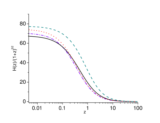
Figure 1: The normalized $H(z)/(1+z)^{3/2}$ in units of km/s/Mpc as a function of the redshift, for $\Lambda$CDM cosmology (black - solid) and for scalar-tensor Model I with $V_{0}=0.06$ and with $G_{5}(X)=\xi X^{2}$, for $\xi=1.7$ (purple - dashed-dotted), $\xi=1.4$ (red - dotted) and $\xi=1.1$ (blue - dashed), in $H_{0}$ units. We have imposed $\Omega_{m0}\approx 0.31$.

Figure 2: Left Graph: The effective dark-energy equation-of-state parameter $w_{DE}$ given in (15) as a function of the redshift, for Model I with $V_{0}=0.08$ and with $\xi=1.3$ in $H_{0}$ units. Right graph: The corresponding normalized effective Newton’s constant $\frac{G_{eff}}{G}$ given in (19) as a function of the redshift. The graphs are from Petronikolou:2021shp .

Finally, let us discuss the perturbative behavior of the model at hand. As one can show DeFelice:2010pv ; DeFelice:2011bh ; Appleby:2011aa , in order for Horndeski/generalized Galileon theory to be free from Laplacian instabilities associated with the scalar field propagation speed one should have

$$c_{S}^{2}\equiv\frac{3(2w_{1}^{2}w_{2}H-w_{2}^{2}w_{4}+4w_{1}w_{2}\dot{w}_{1}-2w_{1}^{2}\dot{w}_{2})}{w_{1}(4w_{1}w_{3}+9w_{2}^{2})}\geq 0,$$ (20)

while in order not to have perturbative ghosts one should have

$$Q_{S}\equiv\frac{w_{1}(4w_{1}w_{3}+9w_{2}^{2})}{3w_{2}^{2}}>0.$$ (21)

Additionally, the light speed in these theories is DeFelice:2011bh

$$c_{T}^{2}\equiv\frac{w_{4}}{w_{1}}\geq 0,$$ (22)

which at late times should be very close to 1, in agreement with LIGO/Virgo bounds Ezquiaga:2017ekz . By studying $c_{S}^{2}$, $Q_{S}$ and $c_{T}^{2}$ one can show that the scenario at hand is viable Petronikolou:2021shp , although with an amount of fine-tuning.

We mention that we could examine other models which can lead to similar behavior, namely a smaller effective Newton’s constant due to the friction term $G_{5}(X)$ that can result to higher $H_{0}$. For instance a model with $G_{5}(X)=\lambda X^{4}$ also leads to $H_{0}\approx 74$ km/s/Mpc for $\lambda=1$ in $H_{0}$ units (since $\lambda$ has dimensions of $[M]^{-17}$ we acquire $\lambda^{1/17}\sim 10^{30}$GeV^-1), and the tension can be alleviated at 3$\sigma$ if $0.5<\lambda<1.2$, in $H_{0}$ units. On the other hand, one can see that models with odd powers of $X$ do not solve the tension, since the last term in (19) changes signs and this does not guarantee that $G_{eff}/G$ will remain smaller than 1.

Finally, we can consider combinations of monomial forms, such as

$$G_{5}(X)=\xi X^{2}+\lambda X^{4},$$ (23)

in which case we have more freedom to obtain the desired decreased $G_{eff}/G$. We elaborate the equations numerically, and in Fig. 3 we present the normalized Hubble constant evolution. As we observe, the $H_{0}$ tension is alleviated due to the decreased effective Newtons’ constant.

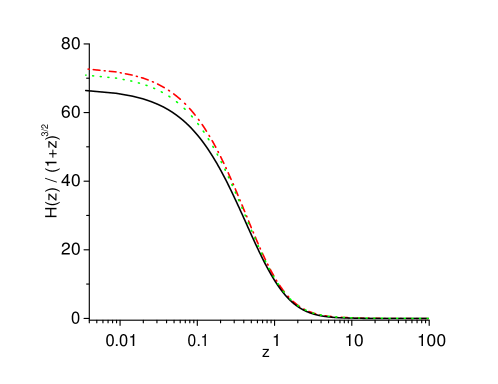
Figure 3: The normalized $H(z)/(1+z)^{3/2}$ in units of km/s/Mpc as a function of the redshift, for $\Lambda$CDM cosmology (black - solid) and for the combined scalar-tensor model (23) with $V_{0}=0.08$ and with $\xi=1.5$, $\lambda=0.001$ (green - dotted), and $\xi=1.3$, $\lambda=0.002$ (red - dashed-dotted), in $H_{0}$ units. We have imposed $\Omega_{m0}\approx 0.31$.

We close this section mentioning that although in modified theories of gravity in general one acquires an effective Newton’s constant different than the standard one, $G_{eff}/G<1$ in a viable way is not easily obtained. For instance, in $f(R)$ gravity where Basilakos:2013nfa

$$\frac{G_{eff}}{G}=\frac{1}{f_{R}}\frac{1+4\frac{k^{2}}{a^{2}}\frac{f_{RR}}{f_{R}}}{1+3\frac{k^{2}}{a^{2}}\frac{f_{RR}}{f_{R}}},$$ (24)

with $k$ the wave-number, one can see that under the viability conditions $f_{,R}>0$ for $R\geq R_{0}$ (with $R_{0}$ the present value of the Ricci scalar) and $f_{,RR}>0$ for $R\geq R_{0}$ DeFelice:2010aj , as well as $0<\frac{Rf_{,RR}}{f_{,R}}(r)<1$ at $r=-\frac{Rf_{,R}}{f}=-2$, DeFelice:2010aj $G_{eff}/G<1$ cannot be obtained. On the other hand, this is indeed possible in $f(T)$ gravity, where $G_{eff}=G\,\left(1+\frac{\partial f(T)}{\partial T}\right)^{-1}$ Nesseris:2013jea . However, scalar-tensor theories may present such behavior quite easily.

In summary, as we see, the above particular sub-class of scalar-tensor gravity can alleviate the $H_{0}$ tension due to the effect of the kinetic-energy-dependent $G_{5}$-term on decreasing $G_{eff}$.

III Bi-scalar-tensor theories alleviating $H_{0}$ tension

In the section we present another class of modified gravity that can lead to the alleviation of $H_{0}$ tension, namely bi-scalar theories of gravity. These theories are determined by the action Naruko:2015zze ; Saridakis:2016ahq

$$S=\int d^{4}\sqrt{-g}\,f\left(R,(\nabla R)^{2},\square R\right),$$ (25)

with $(\nabla R)^{2}=g^{\mu\nu}\nabla_{\mu}R\nabla_{\nu}R$. In this work we focus on models with $f(R,(\nabla R)^{2},\square R)=\mathcal{K}((R,(\nabla R)^{2})+\mathcal{G}(R,(\nabla R)^{2})\square R$. We can rewrite the above action by transforming the Lagrangian using double Lagrange multipliers, in which case one can clearly see that they correspond to bi-scalar-tensor theories of gravity. Hence, introducing the scalar fields $\phi$ and $\chi$ through $g_{\mu\nu}=\frac{1}{2}e^{-\sqrt{\frac{2}{3}}\chi}\hat{g}_{\mu\nu}$ and $\varphi:=f_{\beta}$, with $\beta:=\square R$, we obtain Banerjee:2022ynv

$$\!\!\!\!\!\!\!\!\!\!\!\!\!\!\!S=\int d^{4}x\sqrt{-\hat{g}}\left[\frac{1}{2}\hat{R}-\frac{1}{2}\hat{g}^{\mu\nu}\nabla_{\mu}\chi\nabla_{\nu}\chi\right.-\frac{1}{\sqrt{6}}e^{-\sqrt{\frac{2}{3}}\chi}\hat{g}^{\mu\nu}\mathcal{G}\nabla_{\mu}\chi\nabla_{\nu}\phi+\frac{1}{4}e^{-2\sqrt{\frac{2}{3}}\chi}\mathcal{K}$$

$$\ \ \ \ \ \ \ \ \ \ \ \ \ \ \ \ \left.+\frac{1}{2}e^{-\sqrt{\frac{2}{3}}\chi}\mathcal{G}\hat{\square}\phi-\frac{1}{4}e^{-\sqrt{\frac{2}{3}}\chi}\phi\right].$$ (26)

Thus, varying the above action in terms of the metric, we extract the Friedmann equations as Naruko:2015zze ; Saridakis:2016ahq

$$H^{2}=\frac{1}{3}(\rho_{DE}+\rho_{m})$$ (27)

$$2\dot{H}+3H^{2}=-(p_{DE}+p_{m}),$$ (28)

where we have defined an effective dark-energy sector with energy density and pressure given by

$$\!\!\!\!\!\!\!\!\!\!\!\!\!\!\!\!\!\!\!\!\rho_{DE}:=\frac{1}{2}\dot{\chi}^{2}-\frac{1}{4}e^{-2\sqrt{\frac{2}{3}}\chi}\mathcal{K}-\frac{2}{3}\dot{\phi}^{2}\left[\dot{\phi}\left(\sqrt{6}\dot{\chi}-9H\right)-3\ddot{\phi}\right]\mathcal{G}_{B}$$

$$+\frac{1}{2}e^{-\sqrt{\frac{2}{3}}\chi}\left[\dot{B}\dot{\phi}\mathcal{G}_{B}+\frac{\phi}{2}+\dot{\phi}^{2}\left(\mathcal{G}_{\phi}-2\mathcal{K}_{B}\right)\right],$$ (29)

$$\!\!\!\!\!\!\!\!\!\!\!\!\!\!\!\!\!\!\!\!\!\!\!\!\!\!\!\!\!\!\!\!\!\!\!\!\!\!\!\!\!p_{DE}:=\frac{1}{2}\dot{\chi}^{2}+\frac{1}{4}e^{-2\sqrt{\frac{2}{3}}\chi}\mathcal{K}+\frac{1}{2}e^{-\sqrt{\frac{2}{3}}\chi}\left(\dot{B}\dot{\phi}\mathcal{G}_{B}+\dot{\phi}^{2}\mathcal{G}_{\phi}-\frac{\phi}{2}\right),$$ (30)

with $\mathcal{K}=\mathcal{K}(\phi,B)$ and $\mathcal{G}=\mathcal{G}(\phi,B),$ with $B=2e^{\sqrt{\frac{2}{3}}\chi}g^{\mu\nu}\nabla_{\mu}\phi\nabla_{\nu}\phi,$ and where for simplicity we set the Planck mass to 1. Moreover, varying the action with respect to the scalar fields, we obtain their evolution equation as Naruko:2015zze ; Saridakis:2016ahq :

$$\!\!\!\!\!\!\!\!\!\!\!\!\!\!\!\!\!\!\!\!\!\!\!\!\!\ddot{\chi}+3H\dot{\chi}-\frac{1}{3}\dot{\phi}^{2}\left[\dot{\phi}\left(3\sqrt{6}H-2\dot{\chi}\right)+\sqrt{6}\ddot{\phi}\right]\mathcal{G}_{B}+\frac{1}{\sqrt{6}}e^{-2\sqrt{\frac{2}{3}}\chi}\mathcal{K}$$

$$+\frac{1}{2\sqrt{6}}e^{-\sqrt{\frac{2}{3}}\chi}\left[2\dot{B}\dot{\phi}\mathcal{G}_{B}-\phi+2\dot{\phi}^{2}\left(\mathcal{K}_{B}+\mathcal{G}_{\phi}\right)\right]=0,$$ (31)

and

$$\!\!\!\!\!\!\!\!\!\!\frac{1}{3}e^{-\sqrt{\frac{2}{3}}\chi}\left[\dot{\phi}\left(-9H+\sqrt{6}\dot{\chi}\right)-3\ddot{\phi}\right]\mathcal{K}_{B}+\frac{1}{6}\dot{B}\left\{3e^{-\sqrt{\frac{2}{3}}\chi}\dot{B}+4\dot{\phi}\left[\dot{\phi}\left(9H-\sqrt{6}\dot{\chi}\right)+3\ddot{\phi}\right]\right\}\mathcal{G}_{BB}$$

$$\!\!\!\!\!\!\!\!\!\!+\frac{1}{3}e^{-\sqrt{\frac{2}{3}}\chi}\left[\dot{\phi}\left(9H-\sqrt{6}\dot{\chi}\right)+3\ddot{\phi}\right]\mathcal{G}_{\phi}+\left\{e^{-\sqrt{\frac{2}{3}}\chi}\dot{B}\dot{\phi}+\frac{2}{3}\dot{\phi}^{2}\left[\dot{\phi}\left(9H-\sqrt{6}\dot{\chi}\right)+3\ddot{\phi}\right]\right\}\mathcal{G}_{B\phi}$$

$$\!\!\!\!\!\!\!\!\!\!+\left[\frac{4}{3}\dot{\phi}\left(9H-2\sqrt{6}\dot{\chi}\right)\ddot{\phi}-\frac{1}{\sqrt{6}}e^{-\sqrt{\frac{2}{3}}\chi}\dot{B}\dot{\chi}+\dot{\phi}^{2}\left(18H^{2}+6\dot{H}-3\sqrt{6}H\dot{\chi}-\frac{2}{3}\dot{\chi}^{2}-\sqrt{6}\ddot{\chi}\right)\right]\mathcal{G}_{B}$$

$$\!\!\!\!\!\!\!\!\!\!-e^{-\sqrt{\frac{2}{3}}\chi}\dot{\phi}^{2}\mathcal{K}_{B\phi}+\frac{1}{2}e^{-\sqrt{\frac{2}{3}}\chi}\dot{\phi}^{2}\mathcal{G}_{\phi\phi}-e^{-\sqrt{\frac{2}{3}}\chi}\dot{B}\dot{\phi}\mathcal{K}_{BB}-\frac{1}{4}e^{-2\sqrt{\frac{2}{3}}\chi}\mathcal{K}_{\phi}+\frac{1}{4}e^{-\sqrt{\frac{2}{3}}\chi}=0,$$ (32)

with $\mathcal{G}_{B\phi}=\mathcal{G}_{\phi B}\equiv\frac{\partial^{2}\mathcal{G}}{\partial B\partial\phi}$, etc. Finally, one can define the effective dark-energy equation-of-state parameter as $w_{DE}:=p_{DE}/\rho_{DE}$.

Let us now extract specific models which coincide with $\Lambda$CDM cosmology at CMB redshifts, while at low-redshifts deviate from it, giving rise to higher $H_{0}$. A first model that we can examine is Model I, having

$$\mathcal{K}(\phi,B)=\frac{1}{2}\phi-\frac{\zeta}{2}B\quad\text{and}\quad\mathcal{G}(\phi,B)=0.$$ (33)

In this case, (III),(30) give

$$\rho_{DE}=\frac{1}{2}\dot{\chi}^{2}-\frac{1}{8}e^{-2\sqrt{\frac{2}{3}}\chi}\phi+\frac{1}{4}e^{-\sqrt{\frac{2}{3}}\chi}\left(\phi+\zeta\dot{\phi}^{2}\right),$$ (34)

$$p_{DE}=\frac{1}{2}\dot{\chi}^{2}+\frac{1}{8}e^{-2\sqrt{\frac{2}{3}}\chi}\phi-\frac{1}{4}e^{-\sqrt{\frac{2}{3}}\chi}\left(\phi-\zeta\dot{\phi}^{2}\right).$$ (35)

We solve the cosmological equations numerically and in the left graph of Fig. 4 we depict the normalised combination $H(z)/(1+z)^{3/2}$ as a function of the redshift for $\Lambda$CDM cosmology, and for Model I for different values of $\zeta$. We find that $H_{0}$ depends on the model parameter $\zeta$ as expected, and for $\zeta=-10$ it is around $H_{0}\approx 74km/s/Mpc$, which is consistent with its direct measurement (note that in natural units this corresponds to a typical value $\zeta^{1/4}\sim-10^{-19}$ GeV^-1).

Let us now study what is the mechanism behind the $H_{0}$ alleviation. In the right graph of Fig. 4 we present the evolution of $w_{DE}(z)$, and as we observe most of the time it lies in the phantom regime which, as we discussed in the Introduction, is one of the ways one can obtain the tension alleviation. Hence, contrary to the case of single-scalar-tensor theories of the previous section, where a decreased $G_{eff}$ was the cause of the tension alleviation, in the present bi-scalar theories it is the phantom behavior that leads to higher $H_{0}$.

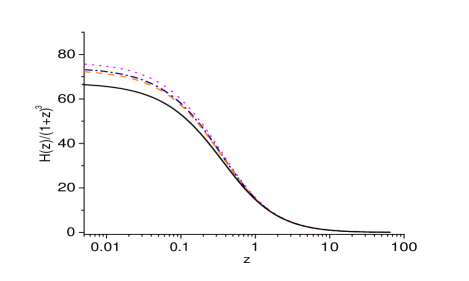
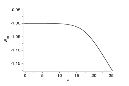
Figure 4: Left Graph: The normalized $H(z)/(1+z)^{3}$ in units of km/s/Mpc as a function of the redshift, for $\Lambda$CDM cosmology (black solid) and for bi-scalar-tensor Model I with $\zeta=-8$ (dashed orange), with $\zeta=-10$ (dashed-dotted blue), and with $\zeta=-12$ (dotted magenta), in Planck units. We have imposed $\Omega_{m0}\approx 0.31$. Right graph: The corresponding effective dark-energy equation-of-state parameter $w_{DE}$ as a function of the redshift, for $\zeta=-10$ in Planck units.

We could proceed to the investigation of other models within the examined class. For instance, we can examine Model II, characterized by

$$\mathcal{K}(\phi,B)=\frac{1}{2}\phi\quad\text{and}\quad\mathcal{G}(\phi,B)=\xi B.$$ (36)

Repeating the same steps as in the previous model we find that the present Hubble value $H_{0}$ depends on the model parameter $\xi$. In particular, for $\xi=-10$ it is around $H_{0}\approx 74km/s/Mpc$ (in natural units $\xi\sim-10$ corresponds to a typical value $\xi^{1/8}\sim-10^{-19}$ GeV^-1). Similarly to the previous case, the mechanism behind the alleviation is the phantom behavior. Hence, we conclude that bi-scalar-tensor theories are very efficient in alleviating the $H_{0}$ tension.

IV Conclusions

We investigated scalar-tensor and bi-scalar-tensor modified theories of gravity that can alleviate the $H_{0}$ tension. In general, gravitational modifications affect the late-time evolution of the universe through the new terms they bring in the Friedmann equations, namely in the effective dark-energy sector, as well as through the effective Newton’s constant they induce. If these effects lead to weaker gravity (smaller $G_{eff}$) at suitable redshifts, or to more repulsive effective dark-energy (for instance exhibiting phantom behavior) then they can cause faster expansion comparing to $\Lambda$CDM paradigm, and thus lead to an increased $H_{0}$ value.

As a first class of models we examined the scalar-tensor theories, namely Horndeski/Generalized Galileon gravity. Choosing particular models with shift-symmetric $G_{5}$ friction term we were able to alleviate the tension by obtaining smaller effective Newton’s constant at intermediate times, a feature that cannot be easily obtained in modified gravity theories. Additionally, we showed that the models at hand are free from perturbative instabilities, and they can have gravitational-wave speed equal to the speed of light, nevertheless with an amount of fine-tuning.

As a second class we examined bi-scalar-tensor theories, namely theories involving two extra propagating degrees of freedom. Choosing particular models we showed that the $H_{0}$ tension can be alleviated, and the mechanism behind it is the phantom behavior of the effective dark-energy equation-of-state parameter.

In summary, as we see, scalar-tensor theories with one or two scalar fields have the capability of alleviating $H_{0}$ tension with both sufficient mechanisms. Such capabilities may be added in the other known phenomenological advantages of these theories, and act as additional indication that they could be good candidates for the description of Nature.

Acknowledgements

M.P. is supported by the Basic Research program of the National Technical University of Athens (NTUA, PEVE) 65232600-ACT-MTG: Alleviating Cosmological Tensions Through Modified Theories of Gravity. The authors acknowledge the contribution of the LISA CosWG, and of COST Actions CA18108 “Quantum Gravity Phenomenology in the multi-messenger approach” and CA21136 “Addressing observational tensions in cosmology with systematics and fundamental physics (CosmoVerse)”.

References

- (1) L. Perivolaropoulos and F. Skara, “Challenges for CDM: An update,” New Astron. Rev. 95 (2022) 101659, arXiv:2105.05208 [astro-ph.CO].
- (2) Planck Collaboration, N. Aghanim et al., “Planck 2018 results. VI. Cosmological parameters,” Astron. Astrophys. 641 (2020) A6, arXiv:1807.06209 [astro-ph.CO]. [Erratum: Astron.Astrophys. 652, C4 (2021)].
- (3) P. Zarrouk et al., “The clustering of the SDSS-IV extended Baryon Oscillation Spectroscopic Survey DR14 quasar sample: measurement of the growth rate of structure from the anisotropic correlation function between redshift 0.8 and 2.2,” Mon. Not. Roy. Astron. Soc. 477 no. 2, (2018) 1639–1663, arXiv:1801.03062 [astro-ph.CO].
- (4) BOSS Collaboration, S. Alam et al., “The clustering of galaxies in the completed SDSS-III Baryon Oscillation Spectroscopic Survey: cosmological analysis of the DR12 galaxy sample,” Mon. Not. Roy. Astron. Soc. 470 no. 3, (2017) 2617–2652, arXiv:1607.03155 [astro-ph.CO].
- (5) E. Di Valentino, O. Mena, S. Pan, L. Visinelli, W. Yang, A. Melchiorri, D. F. Mota, A. G. Riess, and J. Silk, “In the realm of the Hubble tension—a review of solutions,” Class. Quant. Grav. 38 no. 15, (2021) 153001, arXiv:2103.01183 [astro-ph.CO].
- (6) E. Di Valentino, A. Melchiorri, and J. Silk, “Beyond six parameters: extending CDM,” Phys. Rev. D 92 no. 12, (2015) 121302, arXiv:1507.06646 [astro-ph.CO].
- (7) J. L. Bernal, L. Verde, and A. G. Riess, “The trouble with ,” JCAP 10 (2016) 019, arXiv:1607.05617 [astro-ph.CO].
- (8) S. Kumar and R. C. Nunes, “Probing the interaction between dark matter and dark energy in the presence of massive neutrinos,” Phys. Rev. D 94 no. 12, (2016) 123511, arXiv:1608.02454 [astro-ph.CO].
- (9) E. Di Valentino, A. Melchiorri, and O. Mena, “Can interacting dark energy solve the tension?,” Phys. Rev. D 96 no. 4, (2017) 043503, arXiv:1704.08342 [astro-ph.CO].
- (10) E. Di Valentino, C. Bωehm, E. Hivon, and F. R. Bouchet, “Reducing the and tensions with Dark Matter-neutrino interactions,” Phys. Rev. D 97 no. 4, (2018) 043513, arXiv:1710.02559 [astro-ph.CO].
- (11) T. Binder, M. Gustafsson, A. Kamada, S. M. R. Sandner, and M. Wiesner, “Reannihilation of self-interacting dark matter,” Phys. Rev. D 97 no. 12, (2018) 123004, arXiv:1712.01246 [astro-ph.CO].
- (12) E. Di Valentino, A. Melchiorri, E. V. Linder, and J. Silk, “Constraining Dark Energy Dynamics in Extended Parameter Space,” Phys. Rev. D 96 no. 2, (2017) 023523, arXiv:1704.00762 [astro-ph.CO].
- (13) J. Solà, A. Gómez-Valent, and J. de Cruz Pérez, “The tension in light of vacuum dynamics in the Universe,” Phys. Lett. B 774 (2017) 317–324, arXiv:1705.06723 [astro-ph.CO].
- (14) F. D’Eramo, R. Z. Ferreira, A. Notari, and J. L. Bernal, “Hot Axions and the tension,” JCAP 11 (2018) 014, arXiv:1808.07430 [hep-ph].
- (15) V. Poulin, T. L. Smith, T. Karwal, and M. Kamionkowski, “Early Dark Energy Can Resolve The Hubble Tension,” Phys. Rev. Lett. 122 no. 22, (2019) 221301, arXiv:1811.04083 [astro-ph.CO].
- (16) S. Pan, W. Yang, C. Singha, and E. N. Saridakis, “Observational constraints on sign-changeable interaction models and alleviation of the tension,” Phys. Rev. D 100 no. 8, (2019) 083539, arXiv:1903.10969 [astro-ph.CO].
- (17) K. L. Pandey, T. Karwal, and S. Das, “Alleviating the and anomalies with a decaying dark matter model,” JCAP 07 (2020) 026, arXiv:1902.10636 [astro-ph.CO].
- (18) S. Adhikari and D. Huterer, “Super-CMB fluctuations and the Hubble tension,” Phys. Dark Univ. 28 (2020) 100539, arXiv:1905.02278 [astro-ph.CO].
- (19) A. Perez, D. Sudarsky, and E. Wilson-Ewing, “Resolving the tension with diffusion,” Gen. Rel. Grav. 53 no. 1, (2021) 7, arXiv:2001.07536 [astro-ph.CO].
- (20) S. Pan, W. Yang, and A. Paliathanasis, “Non-linear interacting cosmological models after Planck 2018 legacy release and the tension,” Mon. Not. Roy. Astron. Soc. 493 no. 3, (2020) 3114–3131, arXiv:2002.03408 [astro-ph.CO].
- (21) G. Benevento, W. Hu, and M. Raveri, “Can Late Dark Energy Transitions Raise the Hubble constant?,” Phys. Rev. D 101 no. 10, (2020) 103517, arXiv:2002.11707 [astro-ph.CO].
- (22) E. Elizalde, M. Khurshudyan, S. D. Odintsov, and R. Myrzakulov, “Analysis of the tension problem in the Universe with viscous dark fluid,” Phys. Rev. D 102 no. 12, (2020) 123501, arXiv:2006.01879 [gr-qc].
- (23) P. D. Alvarez, B. Koch, C. Laporte, and A. Rincón, “Can scale-dependent cosmology alleviate the tension?,” JCAP 06 (2021) 019, arXiv:2009.02311 [gr-qc].
- (24) B. S. Haridasu, M. Viel, and N. Vittorio, “Sources of -tension in dark energy scenarios,” Phys. Rev. D 103 no. 6, (2021) 063539, arXiv:2012.10324 [astro-ph.CO].
- (25) O. Seto and Y. Toda, “Comparing early dark energy and extra radiation solutions to the Hubble tension with BBN,” Phys. Rev. D 103 no. 12, (2021) 123501, arXiv:2101.03740 [astro-ph.CO].
- (26) J. L. Bernal, L. Verde, R. Jimenez, M. Kamionkowski, D. Valcin, and B. D. Wandelt, “The trouble beyond and the new cosmic triangles,” Phys. Rev. D 103 no. 10, (2021) 103533, arXiv:2102.05066 [astro-ph.CO].
- (27) G. Alestas and L. Perivolaropoulos, “Late-time approaches to the Hubble tension deforming H(z), worsen the growth tension,” Mon. Not. Roy. Astron. Soc. 504 no. 3, (2021) 3956–3962, arXiv:2103.04045 [astro-ph.CO].
- (28) C. Krishnan, R. Mohayaee, E. O. Colgáin, M. M. Sheikh-Jabbari, and L. Yin, “Does Hubble tension signal a breakdown in FLRW cosmology?,” Class. Quant. Grav. 38 no. 18, (2021) 184001, arXiv:2105.09790 [astro-ph.CO].
- (29) A. Theodoropoulos and L. Perivolaropoulos, “The Hubble Tension, the M Crisis of Late Time H(z) Deformation Models and the Reconstruction of Quintessence Lagrangians,” Universe 7 no. 8, (2021) 300, arXiv:2109.06256 [astro-ph.CO].
- (30) B. Hu and M. Raveri, “Can modified gravity models reconcile the tension between the CMB anisotropy and lensing maps in Planck-like observations?,” Phys. Rev. D 91 no. 12, (2015) 123515, arXiv:1502.06599 [astro-ph.CO].
- (31) N. Khosravi, S. Baghram, N. Afshordi, and N. Altamirano, “ tension as a hint for a transition in gravitational theory,” Phys. Rev. D 99 no. 10, (2019) 103526, arXiv:1710.09366 [astro-ph.CO].
- (32) E. Belgacem, Y. Dirian, S. Foffa, and M. Maggiore, “Nonlocal gravity. Conceptual aspects and cosmological predictions,” JCAP 03 (2018) 002, arXiv:1712.07066 [hep-th].
- (33) S. A. Adil, M. R. Gangopadhyay, M. Sami, and M. K. Sharma, “Late-time acceleration due to a generic modification of gravity and the Hubble tension,” Phys. Rev. D 104 no. 10, (2021) 103534, arXiv:2106.03093 [astro-ph.CO].
- (34) R. C. Nunes, “Structure formation in gravity and a solution for tension,” JCAP 05 (2018) 052, arXiv:1802.02281 [gr-qc].
- (35) E. Di Valentino, A. Melchiorri, O. Mena, and S. Vagnozzi, “Nonminimal dark sector physics and cosmological tensions,” Phys. Rev. D 101 no. 6, (2020) 063502, arXiv:1910.09853 [astro-ph.CO].
- (36) S. Vagnozzi, “New physics in light of the tension: An alternative view,” Phys. Rev. D 102 no. 2, (2020) 023518, arXiv:1907.07569 [astro-ph.CO].
- (37) M. Braglia, M. Ballardini, F. Finelli, and K. Koyama, “Early modified gravity in light of the tension and LSS data,” Phys. Rev. D 103 no. 4, (2021) 043528, arXiv:2011.12934 [astro-ph.CO].
- (38) R. D’Agostino and R. C. Nunes, “Measurements of in modified gravity theories: The role of lensed quasars in the late-time Universe,” Phys. Rev. D 101 no. 10, (2020) 103505, arXiv:2002.06381 [astro-ph.CO].
- (39) W. E. V. Barker, A. N. Lasenby, M. P. Hobson, and W. J. Handley, “Systematic study of background cosmology in unitary Poincaré gauge theories with application to emergent dark radiation and tension,” Phys. Rev. D 102 no. 2, (2020) 024048, arXiv:2003.02690 [gr-qc].
- (40) D. Wang and D. Mota, “Can gravity resolve the tension?,” Phys. Rev. D 102 no. 6, (2020) 063530, arXiv:2003.10095 [astro-ph.CO].
- (41) M. Ballardini, M. Braglia, F. Finelli, D. Paoletti, A. A. Starobinsky, and C. Umiltà, “Scalar-tensor theories of gravity, neutrino physics, and the tension,” JCAP 10 (2020) 044, arXiv:2004.14349 [astro-ph.CO].
- (42) F. X. Linares Cedeño and U. Nucamendi, “Revisiting cosmological diffusion models in Unimodular Gravity and the tension,” Phys. Dark Univ. 32 (2021) 100807, arXiv:2009.10268 [astro-ph.CO].
- (43) W. J. C. da Silva and R. Silva, “Cosmological Perturbations in the Tsallis Holographic Dark Energy Scenarios,” Eur. Phys. J. Plus 136 no. 5, (2021) 543, arXiv:2011.09520 [astro-ph.CO].
- (44) S. D. Odintsov, D. Sáez-Chillón Gómez, and G. S. Sharov, “Analyzing the tension in gravity models,” Nucl. Phys. B 966 (2021) 115377, arXiv:2011.03957 [gr-qc].
- (45) E. Abdalla et al., “Cosmology intertwined: A review of the particle physics, astrophysics, and cosmology associated with the cosmological tensions and anomalies,” JHEAp 34 (2022) 49–211, arXiv:2203.06142 [astro-ph.CO].
- (46) CANTATA Collaboration, E. N. Saridakis et al., “Modified Gravity and Cosmology: An Update by the CANTATA Network,” arXiv:2105.12582 [gr-qc].
- (47) S. Capozziello and M. De Laurentis, “Extended Theories of Gravity,” Phys. Rept. 509 (2011) 167–321, arXiv:1108.6266 [gr-qc].
- (48) A. De Felice and S. Tsujikawa, “f(R) theories,” Living Rev. Rel. 13 (2010) 3, arXiv:1002.4928 [gr-qc].
- (49) S. Nojiri and S. D. Odintsov, “Unified cosmic history in modified gravity: from F(R) theory to Lorentz non-invariant models,” Phys. Rept. 505 (2011) 59–144, arXiv:1011.0544 [gr-qc].
- (50) A. A. Starobinsky, “Disappearing cosmological constant in f(R) gravity,” JETP Lett. 86 (2007) 157–163, arXiv:0706.2041 [astro-ph].
- (51) G. Cognola, E. Elizalde, S. Nojiri, S. D. Odintsov, L. Sebastiani, and S. Zerbini, “A Class of viable modified f(R) gravities describing inflation and the onset of accelerated expansion,” Phys. Rev. D 77 (2008) 046009, arXiv:0712.4017 [hep-th].
- (52) L. Amendola and S. Tsujikawa, “Phantom crossing, equation-of-state singularities, and local gravity constraints in f(R) models,” Phys. Lett. B 660 (2008) 125–132, arXiv:0705.0396 [astro-ph].
- (53) A. de la Cruz-Dombriz and A. Dobado, “A f(R) gravity without cosmological constant,” Phys. Rev. D 74 (2006) 087501, arXiv:gr-qc/0607118.
- (54) P. Zhang, “Testing gravity against the large scale structure of the universe.,” Phys. Rev. D 73 (2006) 123504, arXiv:astro-ph/0511218.
- (55) V. Faraoni, “de Sitter space and the equivalence between f(R) and scalar-tensor gravity,” Phys. Rev. D 75 (2007) 067302, arXiv:gr-qc/0703044.
- (56) S. Basilakos, S. Nesseris, and L. Perivolaropoulos, “Observational constraints on viable f(R) parametrizations with geometrical and dynamical probes,” Phys. Rev. D 87 no. 12, (2013) 123529, arXiv:1302.6051 [astro-ph.CO].
- (57) T. Papanikolaou, C. Tzerefos, S. Basilakos, and E. N. Saridakis, “Scalar induced gravitational waves from primordial black hole Poisson fluctuations in f(R) gravity,” JCAP 10 (2022) 013, arXiv:2112.15059 [astro-ph.CO].
- (58) S. Nojiri and S. D. Odintsov, “Modified Gauss-Bonnet theory as gravitational alternative for dark energy,” Phys. Lett. B 631 (2005) 1–6, arXiv:hep-th/0508049.
- (59) A. De Felice and S. Tsujikawa, “Construction of cosmologically viable f(G) dark energy models,” Phys. Lett. B 675 (2009) 1–8, arXiv:0810.5712 [hep-th].
- (60) Y.-Y. Zhao, Y.-B. Wu, J.-B. Lu, Z. Zhang, W.-L. Han, and L.-L. Lin, “Modified f(G) gravity models with curvature-matter coupling,” Eur. Phys. J. C 72 (2012) 1924, arXiv:1203.5593 [astro-ph.CO].
- (61) M. F. Shamir and T. Naz, “Stellar structures in f(G) gravity admitting Noether symmetries,” Phys. Lett. B 806 (2020) 135519, arXiv:2006.03339 [gr-qc].
- (62) P. Asimakis, S. Basilakos, and E. N. Saridakis, “Building cubic gravity with healthy and viable scalar and tensor perturbations,” arXiv:2212.12494 [gr-qc].
- (63) D. Lovelock, “The Einstein tensor and its generalizations,” J. Math. Phys. 12 (1971) 498–501.
- (64) N. Deruelle and L. Farina-Busto, “The Lovelock Gravitational Field Equations in Cosmology,” Phys. Rev. D 41 (1990) 3696.
- (65) Y.-F. Cai, S. Capozziello, M. De Laurentis, and E. N. Saridakis, “f(T) teleparallel gravity and cosmology,” Rept. Prog. Phys. 79 no. 10, (2016) 106901, arXiv:1511.07586 [gr-qc].
- (66) G. R. Bengochea and R. Ferraro, “Dark torsion as the cosmic speed-up,” Phys. Rev. D 79 (2009) 124019, arXiv:0812.1205 [astro-ph].
- (67) E. V. Linder, “Einstein’s Other Gravity and the Acceleration of the Universe,” Phys. Rev. D 81 (2010) 127301, arXiv:1005.3039 [astro-ph.CO]. [Erratum: Phys.Rev.D 82, 109902 (2010)].
- (68) S.-H. Chen, J. B. Dent, S. Dutta, and E. N. Saridakis, “Cosmological perturbations in f(T) gravity,” Phys. Rev. D 83 (2011) 023508, arXiv:1008.1250 [astro-ph.CO].
- (69) N. Tamanini and C. G. Boehmer, “Good and bad tetrads in f(T) gravity,” Phys. Rev. D 86 (2012) 044009, arXiv:1204.4593 [gr-qc].
- (70) G. R. Bengochea, “Observational information for f(T) theories and Dark Torsion,” Phys. Lett. B 695 (2011) 405–411, arXiv:1008.3188 [astro-ph.CO].
- (71) D. Liu and M. J. Reboucas, “Energy conditions bounds on f(T) gravity,” Phys. Rev. D 86 (2012) 083515, arXiv:1207.1503 [astro-ph.CO].
- (72) M. H. Daouda, M. E. Rodrigues, and M. J. S. Houndjo, “Anisotropic fluid for a set of non-diagonal tetrads in f(T) gravity,” Phys. Lett. B 715 (2012) 241–245, arXiv:1202.1147 [gr-qc].
- (73) H. Mohseni Sadjadi, “Generalized Noether symmetry in f(T) gravity,” Phys. Lett. B 718 (2012) 270–275, arXiv:1210.0937 [gr-qc].
- (74) A. Finch and J. L. Said, “Galactic Rotation Dynamics in f(T) gravity,” Eur. Phys. J. C 78 no. 7, (2018) 560, arXiv:1806.09677 [astro-ph.GA].
- (75) A. Golovnev and M.-J. Guzmán, “Bianchi identities in gravity: Paving the way to confrontation with astrophysics,” Phys. Lett. B 810 (2020) 135806, arXiv:2006.08507 [gr-qc].
- (76) C. Bejarano, R. Ferraro, and M. J. Guzmán, “Kerr geometry in f(T) gravity,” Eur. Phys. J. C 75 (2015) 77, arXiv:1412.0641 [gr-qc].
- (77) F. Darabi and K. Atazadeh, “f(T) quantum cosmology,” Phys. Rev. D 100 no. 2, (2019) 023546, arXiv:1903.03409 [gr-qc].
- (78) S. Sahlu, J. Ntahompagaze, M. Elmardi, and A. Abebe, “The Chaplygin gas as a model for modified teleparallel gravity?,” Eur. Phys. J. C 79 no. 9, (2019) 749, arXiv:1904.09897 [gr-qc].
- (79) M. Benetti, S. Capozziello, and G. Lambiase, “Updating constraints on f(T) teleparallel cosmology and the consistency with Big Bang Nucleosynthesis,” Mon. Not. Roy. Astron. Soc. 500 no. 2, (2020) 1795–1805, arXiv:2006.15335 [astro-ph.CO].
- (80) A. Golovnev and M.-J. Guzmán, “Approaches to spherically symmetric solutions in f(T) gravity,” Universe 7 no. 5, (2021) 121, arXiv:2103.16970 [gr-qc].
- (81) L. K. Duchaniya, S. V. Lohakare, B. Mishra, and S. K. Tripathy, “Dynamical stability analysis of accelerating f(T) gravity models,” Eur. Phys. J. C 82 no. 5, (2022) 448, arXiv:2202.08150 [gr-qc].
- (82) G. Kofinas and E. N. Saridakis, “Teleparallel equivalent of Gauss-Bonnet gravity and its modifications,” Phys. Rev. D 90 (2014) 084044, arXiv:1404.2249 [gr-qc].
- (83) G. Kofinas and E. N. Saridakis, “Cosmological applications of gravity,” Phys. Rev. D 90 (2014) 084045, arXiv:1408.0107 [gr-qc].
- (84) S. Bahamonde, C. G. Böhmer, and M. Wright, “Modified teleparallel theories of gravity,” Phys. Rev. D 92 no. 10, (2015) 104042, arXiv:1508.05120 [gr-qc].
- (85) G. Farrugia, J. Levi Said, V. Gakis, and E. N. Saridakis, “Gravitational Waves in Modified Teleparallel Theories,” Phys. Rev. D 97 no. 12, (2018) 124064, arXiv:1804.07365 [gr-qc].
- (86) C. Escamilla-Rivera and J. Levi Said, “Cosmological viable models in theory as solutions to the tension,” Class. Quant. Grav. 37 no. 16, (2020) 165002, arXiv:1909.10328 [gr-qc].
- (87) M. Caruana, G. Farrugia, and J. Levi Said, “Cosmological bouncing solutions in gravity,” Eur. Phys. J. C 80 no. 7, (2020) 640, arXiv:2007.09925 [gr-qc].
- (88) A. R. P. Moreira, J. E. G. Silva, F. C. E. Lima, and C. A. S. Almeida, “Thick brane in f(T,B) gravity,” Phys. Rev. D 103 no. 6, (2021) 064046, arXiv:2101.10054 [hep-th].
- (89) G. W. Horndeski, “Second-order scalar-tensor field equations in a four-dimensional space,” Int. J. Theor. Phys. 10 (1974) 363–384.
- (90) A. De Felice and S. Tsujikawa, “Generalized Galileon cosmology,” Phys. Rev. D 84 (2011) 124029, arXiv:1008.4236 [hep-th].
- (91) C. Deffayet, X. Gao, D. A. Steer, and G. Zahariade, “From k-essence to generalised Galileons,” Phys. Rev. D 84 (2011) 064039, arXiv:1103.3260 [hep-th].
- (92) D. F. Mota, M. Sandstad, and T. Zlosnik, “Cosmology of the selfaccelerating third order Galileon,” JHEP 12 (2010) 051, arXiv:1009.6151 [astro-ph.CO].
- (93) A. Barreira, B. Li, W. A. Hellwing, C. M. Baugh, and S. Pascoli, “Nonlinear structure formation in the Cubic Galileon gravity model,” JCAP 10 (2013) 027, arXiv:1306.3219 [astro-ph.CO].
- (94) T. Qiu, J. Evslin, Y.-F. Cai, M. Li, and X. Zhang, “Bouncing Galileon Cosmologies,” JCAP 10 (2011) 036, arXiv:1108.0593 [hep-th].
- (95) S. A. Appleby and E. V. Linder, “Trial of Galileon gravity by cosmological expansion and growth observations,” JCAP 08 (2012) 026, arXiv:1204.4314 [astro-ph.CO].
- (96) A. Barreira, B. Li, C. Baugh, and S. Pascoli, “The observational status of Galileon gravity after Planck,” JCAP 08 (2014) 059, arXiv:1406.0485 [astro-ph.CO].
- (97) F. Arroja, N. Bartolo, P. Karmakar, and S. Matarrese, “The two faces of mimetic Horndeski gravity: disformal transformations and Lagrange multiplier,” JCAP 09 (2015) 051, arXiv:1506.08575 [gr-qc].
- (98) K. Hinterbichler and A. Joyce, “Hidden symmetry of the Galileon,” Phys. Rev. D 92 no. 2, (2015) 023503, arXiv:1501.07600 [hep-th].
- (99) E. Babichev, C. Charmousis, and M. Hassaine, “Charged Galileon black holes,” JCAP 05 (2015) 031, arXiv:1503.02545 [gr-qc].
- (100) P. Brax, C. Burrage, and A.-C. Davis, “Laboratory Tests of the Galileon,” JCAP 09 (2011) 020, arXiv:1106.1573 [hep-ph].
- (101) J. Renk, M. Zumalacárregui, F. Montanari, and A. Barreira, “Galileon gravity in light of ISW, CMB, BAO and H0 data,” JCAP 10 (2017) 020, arXiv:1707.02263 [astro-ph.CO].
- (102) J. Gleyzes, D. Langlois, F. Piazza, and F. Vernizzi, “Healthy theories beyond Horndeski,” Phys. Rev. Lett. 114 no. 21, (2015) 211101, arXiv:1404.6495 [hep-th].
- (103) D. Langlois and K. Noui, “Degenerate higher derivative theories beyond Horndeski: evading the Ostrogradski instability,” JCAP 02 (2016) 034, arXiv:1510.06930 [gr-qc].
- (104) D. Langlois, “Dark energy and modified gravity in degenerate higher-order scalar–tensor (DHOST) theories: A review,” Int. J. Mod. Phys. D 28 no. 05, (2019) 1942006, arXiv:1811.06271 [gr-qc].
- (105) E. Babichev, C. Charmousis, and A. Lehébel, “Asymptotically flat black holes in Horndeski theory and beyond,” JCAP 04 (2017) 027, arXiv:1702.01938 [gr-qc].
- (106) A. Ilyas, M. Zhu, Y. Zheng, Y.-F. Cai, and E. N. Saridakis, “DHOST Bounce,” JCAP 09 (2020) 002, arXiv:2002.08269 [gr-qc].
- (107) A. Naruko, D. Yoshida, and S. Mukohyama, “Gravitational scalar–tensor theory,” Class. Quant. Grav. 33 no. 9, (2016) 09LT01, arXiv:1512.06977 [gr-qc].
- (108) E. N. Saridakis and M. Tsoukalas, “Cosmology in new gravitational scalar-tensor theories,” Phys. Rev. D 93 no. 12, (2016) 124032, arXiv:1601.06734 [gr-qc].
- (109) L. Heisenberg, H. Villarrubia-Rojo, and J. Zosso, “Simultaneously solving the H0 and 8 tensions with late dark energy,” Phys. Dark Univ. 39 (2023) 101163, arXiv:2201.11623 [astro-ph.CO].
- (110) L. Heisenberg, H. Villarrubia-Rojo, and J. Zosso, “Can late-time extensions solve the H0 and 8 tensions?,” Phys. Rev. D 106 no. 4, (2022) 043503, arXiv:2202.01202 [astro-ph.CO].
- (111) A. De Felice and S. Tsujikawa, “Conditions for the cosmological viability of the most general scalar-tensor theories and their applications to extended Galileon dark energy models,” JCAP 02 (2012) 007, arXiv:1110.3878 [gr-qc].
- (112) T. Kobayashi, M. Yamaguchi, and J. Yokoyama, “Generalized G-inflation: Inflation with the most general second-order field equations,” Prog. Theor. Phys. 126 (2011) 511–529, arXiv:1105.5723 [hep-th].
- (113) M. Petronikolou, S. Basilakos, and E. N. Saridakis, “Alleviating tension in Horndeski gravity,” arXiv:2110.01338 [gr-qc].
- (114) E. N. Saridakis and S. V. Sushkov, “Quintessence and phantom cosmology with non-minimal derivative coupling,” Phys. Rev. D 81 (2010) 083510, arXiv:1002.3478 [gr-qc].
- (115) G. Koutsoumbas, K. Ntrekis, E. Papantonopoulos, and E. N. Saridakis, “Unification of Dark Matter - Dark Energy in Generalized Galileon Theories,” JCAP 02 (2018) 003, arXiv:1704.08640 [gr-qc].
- (116) S. Karydas, E. Papantonopoulos, and E. N. Saridakis, “Successful Higgs inflation from combined nonminimal and derivative couplings,” Phys. Rev. D 104 no. 2, (2021) 023530, arXiv:2102.08450 [gr-qc].
- (117) E. Bellini and I. Sawicki, “Maximal freedom at minimum cost: linear large-scale structure in general modifications of gravity,” JCAP 07 (2014) 050, arXiv:1404.3713 [astro-ph.CO].
- (118) S. Peirone, K. Koyama, L. Pogosian, M. Raveri, and A. Silvestri, “Large-scale structure phenomenology of viable Horndeski theories,” Phys. Rev. D 97 no. 4, (2018) 043519, arXiv:1712.00444 [astro-ph.CO].
- (119) A. De Felice and S. Tsujikawa, “Cosmology of a covariant Galileon field,” Phys. Rev. Lett. 105 (2010) 111301, arXiv:1007.2700 [astro-ph.CO].
- (120) S. Appleby and E. V. Linder, “The Paths of Gravity in Galileon Cosmology,” JCAP 03 (2012) 043, arXiv:1112.1981 [astro-ph.CO].
- (121) J. M. Ezquiaga and M. Zumalacárregui, “Dark Energy After GW170817: Dead Ends and the Road Ahead,” Phys. Rev. Lett. 119 no. 25, (2017) 251304, arXiv:1710.05901 [astro-ph.CO].
- (122) S. Nesseris, S. Basilakos, E. N. Saridakis, and L. Perivolaropoulos, “Viable models are practically indistinguishable from CDM,” Phys. Rev. D 88 (2013) 103010, arXiv:1308.6142 [astro-ph.CO].
- (123) S. Banerjee, M. Petronikolou, and E. N. Saridakis, “Alleviating the H0 tension with new gravitational scalar tensor theories,” Phys. Rev. D 108 no. 2, (2023) 024012, arXiv:2209.02426 [gr-qc].