Quasinormal modes of Reissner-Nordström–AdS: the approach to extremality

Abstract

We consider the quasinormal spectrum of scalar and gravitational perturbations of the Reissner-Nordström–AdS black hole as the horizon approaches extremality. By considering a foliation of the black hole by spacelike surfaces which intersect the future horizon we implement numerical methods which are well behaved up to and including the extremal limit and which admit initial data which is nontrivial at the horizon. As extremality is approached we observe a transition whereby the least damped mode ceases to be oscillatory in time, and the late time signal changes qualitatively as a consequence.

1 Introduction

Numerical [8, 4] and observational [1] evidence shows that a black hole spacetime will, in response to a perturbation, produce radiation at (complex) frequencies which are characteristic of the black hole. These frequencies are the quasinormal frequencies, and to each such frequency is associated a quasinormal mode – a solution of a linear equation on the black hole background, satisfying suitable boundary conditions at any horizons and (if relevant) at null infinity [27, 5, 28].

In recent years, a satisfactory mathematical understanding of the quasinormal modes of subextremal de Sitter black hole spacetimes has developed, starting with results for Schwarzschild-de Sitter [33, 7], culminating in a general theory for de Sitter black holes [35] including the full subextremal range of Kerr–de Sitter black holes [11, 31]. In the subextremal anti-de Sitter setting, analogous results have been shown [37, 17]. For a thorough overview see [12], and for an explicit worked example using this approach, see [6].

The majority of the works cited in the previous paragraph impose regularity at the future horizon(s) in order to characterise the quasinormal modes, an approach which in the physics literature goes back to Schmidt [34]. It can be shown that time-harmonic solutions to the linearised equations which extend smoothly across the future horizons exist only for a discrete set of complex frequencies, which can be identified with the quasinormal frequencies. Regularity at the horizon plays the role of ‘in/outgoing’ boundary conditions in more traditional treatments. This approach breaks down when the black hole horizon is extremal or the spacetime is asymptotically flat. (For the purposes of our discussion, an asymptotically flat end may be thought of as the extremal limit of a subextremal cosmological horizon, and when we refer to a subextremal spacetime we implicitly assume that it has no asymptotically flat ends).

The behaviour of the quasinormal spectrum as a spacetime approaches extremality has been the topic of significant interest in the physics literature [20]-[25], [39], [40]. In particular, going back at least to Detweiler [10], two distinct behaviours have been observed for the quasinormal frequencies as the surface gravity, $\kappa$ approaches zero. Firstly, it appears that a generic feature of near-extremal spacetimes is the existence of a sequence of ‘zero damped modes’ with damping rates approximately $n\kappa$, $n=1,2,3,\ldots$, which accumulate at some given frequency in the limit $\kappa\to 0$. On the other hand, in certain regions of the complex frequency plane, the quasinormal frequencies are largely unaffected by the extremal limit – the frequencies settle down to limiting values without accumulating (called ‘damped modes’).

In [14] the second author, together with Gajic, considered the Reissner-Nordström-de Sitter black hole and showed that in the limit where both horizons become extremal there is a sector in the complex plane in which, away from the origin, only the damped mode behaviour is observed. In [26] Joykutty established the existence of purely damped modes in several situations involving a horizon approaching extremality, including that of the Reissner–Nordström-de Sitter black hole with either horizon becoming extremal (see also [18, 19] for a closely related result).

In this paper, we aim to study numerically the quasinormal spectrum of the Reissner-Nordström–anti-de Sitter black hole in the approach to extremality. Our approach is motivated by that taken in [13, 14], and involves working in coordinates which are regular at the horizon (see [15] for an alternative approach). We first briefly consider a scalar toy equation which can be solved explicitly in terms of special functions in order to verify our numerical methods, before moving on to study the conformal wave equation and the scalar and axial gravitational perturbations for the Reissner-Nordström–anti-de Sitter black hole as the horizon approaches extremality.

We work both in the time and frequency domains, enabling cross-checking of results between independent computations. In the time domain our choice of slicing permits us to simulate time evolution up to and including the horizon, without introducing any artificial boundaries. In the frequency domain we use a modified Leaver method to determine quasinormal frequencies (this was demonstrated to correctly locate the quasinormal frequencies in [13]). In both cases our methods are designed such that there is no degeneration as $\kappa\to 0$ and so that we are able to consider initial data which is non-trivial at the future event horizon.

Our approach enables us to extend the numerical results of [3] to the full parameter range, up to and including extremality. A particularly interesting feature we observe for both the conformal wave equation and the gravitational perturbations is a threshold in parameter space at which the qualitative behaviour of the fields changes. This happens when the surface gravity is sufficiently small that the slowest decaying purely damped mode becomes the dominant late-time behaviour. On one side of this threshold the late time behaviour is oscillatory, but closer to extremality the dominant behaviour becomes pure exponential decay. In the extremal limit, this ever-slower exponential decay becomes the polynomial decay expected for an extremal black hole [41].

Acknowledgements

We are grateful to the Erwin Schrödinger International Institute for Mathematics and Physics, where some of this work was undertaken during the Thematic Programme “Spectral Theory and Mathematical Relativity”. FF acknowledges support by Polish National Science Centre Grant No. 2020/36/T/ST2 /00323 and the Austrian Science Fund (FWF) via Project P 36455.

2 Explicitly solvable toy-model

We consider the following equation which models the behaviour of a wave exterior to an extremal AdS black hole:

$$-\partial_{t}^{2}\psi+\partial_{x}(x^{2}\partial_{x}\psi)+2\partial_{t}\partial_{x}\psi+\partial_{\theta}^{2}\psi+\frac{1}{4}\psi=0.$$ (1)

where $(t,x,\theta)\in[0,T)\times[0,1]\times S^{1}$. The principle part of this operator agrees with that of the wave operator for the spacetime with metric $g$ given by

$$g^{-1}=-\frac{\partial}{\partial t}\otimes\frac{\partial}{\partial t}+\frac{\partial}{\partial t}\otimes\frac{\partial}{\partial x}+\frac{\partial}{\partial x}\otimes\frac{\partial}{\partial t}+x^{2}\frac{\partial}{\partial x}\otimes\frac{\partial}{\partial x}+\frac{\partial}{\partial\theta}\otimes\frac{\partial}{\partial\theta}$$ (2)

The causal diagram of this spacetime is shown in Fig. 1. It enjoys the presence of an extremal horizon at $x=0$, as can be seen from the fact that $g(\partial_{t},\partial_{t})$ behaves like $x^{2}$ in its vicinity. Let us point out that the time coordinate variable is chosen in such a way that the surfaces of constant time $t$ penetrate this horizon and the metric extends smoothly across $x=0$.

Figure 1: Causal diagram for the spacetime described by Eq. (2). The angular dimension is suppressed.

In this section we investigate solutions to Eq. (1) satisfying the Dirichlet condition $\psi(t,1,\theta)=0$ at $x=1$. At $x=0$ we do not require a boundary condition, owing to the presence of the horizon. We assume that initial conditions $\psi(0,x,\theta)$ and $\partial_{t}\psi(0,x,\theta)$ are specified.

According to the prescription of [13, 14], in order to find the quasinormal frequencies of Eq. (1) we should seek solutions to the equation of the form

$$\psi(t,x,\theta)=e^{st+im\theta}u(x)$$

which satisfy the boundary condition at $x=1$ and which have improved regularity (relative to a generic solution) at $x=0$. Here we have made use of the rotational symmetry to restrict attention to a single angular mode. The function $u$ can be seen to satisfy the following ODE

$$-\frac{d}{dx}\left(x^{2}\frac{d}{dx}u\right)-2s\frac{d}{dx}u+\left(s^{2}+m^{2}-\frac{1}{4}\right)u=0.$$ (3)

Introducing a function $v$ given by

$$u(x)=e^{\frac{s}{x}}\sqrt{\frac{s}{x}}v\left(\frac{s}{x}\right),$$

the left hand side of Eq. (3) becomes the modified Bessel equation

$$z^{2}\frac{d^{2}v}{dz^{2}}+z\frac{dv}{dz}-\left(z^{2}+\lambda^{2}\right)v=0,$$

where $z=\frac{s}{x}$ and $\lambda=\sqrt{s^{2}+m^{2}}$. Thus, the general solution of (3) can be written as

$$u(x)=e^{\frac{s}{x}}\sqrt{\frac{s}{x}}\left(a\,K_{\lambda}\left(\frac{s}{x}\right)+b\,I_{\lambda}\left(\frac{s}{x}\right)\right),$$ (4)

where $a,b\in\mathbb{C}$ and $I_{\lambda}(z),K_{\lambda}(z)$ are the modified Bessel functions of the first and second kind respectively [38].

In order to discuss the regularity condition that we impose at $x=0$, recall that a smooth function $f:(0,1)\to\mathbb{C}$ is $(\sigma,k)-$Gevrey regular with $\sigma,k>0$ if there exists a constant $C$ such that

$$\sup_{x\in(0,1)}\left|f^{(n)}(x)\right|\leqslant C\sigma^{-n}(n!)^{k}.$$

Note that for fixed $k$, increasing $\sigma$ imposes a more stringent regularity condition on $f$.

By a careful analysis of the asymptotic series of the modified Bessel functions using the approach of [38, §7.31], together with [2, Prop 8] and [15, eqn (A.1)] it is possible to show that for fixed $s$ with $|\arg s|<\pi$:

• $e^{\frac{s}{x}}\sqrt{\frac{s}{x}}\,K_{\lambda}\left(\frac{s}{x}\right)$ is $(\sigma,2)-$Gevrey regular for any $\sigma<|s|$

• $e^{\frac{s}{x}}\sqrt{\frac{s}{x}}\,I_{\lambda}\left(\frac{s}{x}\right)$ is not $(\sigma,2)-$Gevrey regular if $\left\{\begin{array}[]{ll}\sigma>0,&|\arg s|\leqslant\pi/2\\ \sigma>|s|-|\Im(s)|,&\pi/2<|\arg s|<\pi\end{array}\right.$

In particular, this implies that we should make the choice $b=0$ in (4) to single out the more regular branch of solutions (in the Gevrey sense) at $x=0$. In order that our solution also satisfies the boundary condition at $x=1$ we require

$$K_{\sqrt{s^{2}+m^{2}}}(s)=0.$$ (5)

Thus the quasinormal frequencies are precisely the solutions to Eq. (5). Since $K_{\lambda}(z)$ is an entire, even, function of $\lambda$, the branch points at $\pm im$ are removable, however, a branch point at $s=0$ will be present in general.

The solutions of Eq. (5) for various $m$ are given in Table 1 and presented in Fig. 2. As well as the locations of the quasinormal frequencies, we also obtain an explicit formula for the corresponding quasinormal modes:

$$\psi(t,x,\theta)=e^{st+im\theta+\frac{s}{x}}\sqrt{\frac{s}{x}}K_{\sqrt{s^{2}+m^{2}}}\left(\frac{s}{x}\right),$$

where $s$ is a solution to Eq. (5).

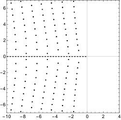
Figure 2: Locations of the lowest solutions to Eq. (5) in the complex plane. The dashed line represents the branch cut.

$m=0$
$m=1$
$m=2$	$-1.060\pm 0.736i$
$m=3$	$-1.167\pm 1.441i$	$-2.302\pm 0.371i$
$m=4$	$-1.258\pm 2.122i$	$-2.382\pm 1.216i$
$m=5$	$-1.337\pm 2.798i$	$-2.494\pm 1.965i$	$-3.624\pm 0.842i$
$m=6$	$-1.407\pm 3.473i$	$-2.603\pm 2.675i$	$-3.709\pm 1.685i$	$-4.934\pm 0.382i$
$m=7$	$-1.471\pm 4.149i$	$-2.705\pm 3.367i$	$-3.819\pm 2.457i$	$-4.951\pm 1.310i$
$m=8$	$-1.529\pm 4.826i$	$-2.800\pm 4.053i$	$-3.931\pm 3.191i$	$-5.038\pm 2.151i$	$-6.239\pm 0.869i$

Table 1: Approximate quasinormal frequencies for Eq. (1).

The presented results can be confronted with the numerical approach. Equation (1) can be solved with the use of the pseudospectral scheme. Since at $x=1$ we impose the Dirichlet condition, to control it we employ the Gauss-Radau quadratures. The solutions that we are looking for are decaying exponentially with time in the quasinormal regime. Hence, to improve the precision of the scheme one can evolve an auxiliary function $\tilde{\psi}(t,x,\theta)=e^{\alpha t}\psi(t,x,\theta)$ with $\alpha>0$ being a suitably chosen constant. The accuracy of this method can be controlled by the energy

$$E(t)=\frac{1}{2}\int_{0}^{1}\int_{0}^{2\pi}\left[|\partial_{t}\psi|^{2}+x^{2}|\partial_{x}\psi|^{2}+|\partial_{\theta}\psi|^{2}-\frac{1}{4}|\psi|^{2}\right]dx\,d\theta.$$

One can use the Hardy inequality to show that it is positive. Due to the absence of term $\partial_{t}\psi$ in Eq. (1) and the coefficient next to $\partial_{\tau x}$ being constant, this energy changes in time only via the leakage through the horizon. This change is given by a simple expression involving only an integration over the angular variable

$$E^{\prime}(t)=-\int_{0}^{2\pi}|\partial_{t}\psi|^{2}_{x=0}\,d\theta.$$

As can be seen in Fig. 3 for larger values of $m$ one can easily observe the quasinormal regime. The quasinormal frequencies obtained via fitting agree with the lowest values from Table 1. Note that the initial data is chosen to be non-zero at the horizon – a key feature of the approach of [13, 14] is that such initial data is permissible.

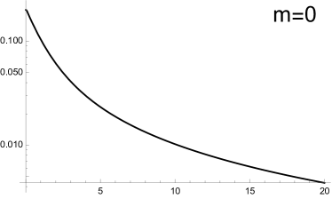
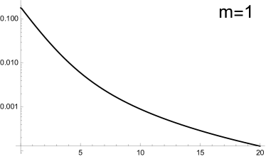
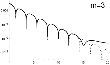
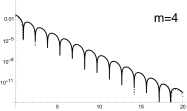
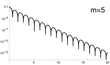
Figure 3: Plots of solutions to Eq. (1) for the initial data $\phi(0,x,\theta)=(1-x)\cos m\theta$, $\phi_{t}(0,x,\theta)=0$ with various $m$. The solid lines show functions $|\phi(t,0.8,\frac{\pi}{7})|$ and the dotted lines represent the fitted dominating quasinormal mode.

An alternative approach to finding the quasinormal modes frequencies for our toy-model is by the Leaver method [29, 30]. Let us fix some angular number $m$ and again look for solutions of the form $\psi(t,x,\theta)=e^{st}e^{im\theta}u(x)$. Then $u$ satisfies Eq. (3) and we can expand it into a Taylor series around $x=1$: $u(x)=\sum_{k=0}^{\infty}H_{k}(1-x)^{k}$. The coefficients $H_{k}$ must satisfy the following recurrence relation

$$H_{k}=\frac{1}{(k-1)k}\left[2(k-1)(k-1+s)H_{k-1}-\left((k-2)(k-1)-\left(s^{2}+m^{2}-\frac{1}{4}\right)\right)H_{k-2}\right]$$ (6)

for $k\geq 2$. Since we impose the Dirichlet condition at $x=1$, we need to set $H_{0}=0$. The regularity condition at $x=0$ suggests that $H_{k}$ should converge to zero as $k\to\infty$. It gives us a quantization condition on $s$. One can obtain the appropriate values of $s$ using the method of continued fractions, but in our case it is enough to assume that for some sufficiently large value of $n$ one has $H_{n}=0$. It leads to a polynomial, whose zeroes include approximations to $s$ we seek and many superfluous values. To identify the correct values of $s$ one can change $n$ and see which roots converge. It is presented in Fig. 4. From the analytical solution to the toy model we know that proper quasinormal frequencies have non-zero imaginary part (red dots in the plot). Quasinormal frequencies obtained with this method agree with the ones resulting from Eq. (5).

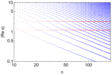
Figure 4: Log-log plot of absolute values of real parts of solutions to equation $H_{n}=0$ for various values of $n$, where $H_{n}$ is given by the recurrence relation (6). Blue dots show spurious solutions that are purely real, while the red ones have non-trivial imaginary part and converge to the quasinormal frequencies.

3 Reissner-Nordström-anti-de Sitter black hole

Now we would like to apply the same methods to study the quasinormal modes in the Reissner-Nordström-anti-de Sitter (RNAdS) spacetime. Let us start by investigating the wave operator in this spacetime. Our first step consists of finding a suitable coordinate system in which it becomes similar to the one from the toy model.

In spherical cooridnates $(t,r,\theta,\phi)$ the line element of the RNAdS spacetime is given by

$$ds^{2}=-\left(1-\frac{2M}{r}+\frac{Q^{2}}{r^{2}}+\frac{r^{2}}{\ell^{2}}\right)dt^{2}+\left(1-\frac{2M}{r}+\frac{Q^{2}}{r^{2}}+\frac{r^{2}}{\ell^{2}}\right)^{-1}dr^{2}+r^{2}d\Omega^{2},$$ (7)

where $d\Omega^{2}$ is a line element on a two-dimensional unit sphere. The values of $M$ and $Q$ are interpreted as the mass and the charge of the black hole, respectively, while $\ell$ gives a specific length-scale connected with the cosmological constant $\Lambda$ via $\Lambda=-3/\ell^{2}$. In the generic case this spacetime has two spherical horizons called the Cauchy horizon (of a radius $r_{C}$) and the event horizon (of a radius $r_{H}$). However, if $Q=0$, the latter vanishes and we get a Schwarzschild-anti-de Sitter spacetime. On the other hand, for $Q$ large enough these horizons coincide, i.e., $r_{H}=r_{C}=(3M-\sqrt{9M^{2}-8Q^{2}})/2$ and then their position does not depend on the cosmological constant. This situation is called an extremal case, in contrast to the regular case in which $r_{C}<r_{H}$. In the following we want to cover both regular and extremal cases so we need a framework that will suitably handle both possibilites. For this purpose it is convenient to introduce the following quantities. Let $\rho=r/r_{H}$ be a new radial variable and $t_{H}=t/r_{H}$ a new temporal variable. We also define the parameters $\sigma=r_{C}/r_{H}$, and $\lambda=r_{H}^{2}/\ell^{2}$. Then Eq. (7) can be written as

$$ds^{2}=r_{H}^{2}\left[-f(\rho)dt_{H}^{2}+f(\rho)^{-1}d\rho^{2}+\rho^{2}d\Omega^{2}\right]$$ (8)

where

$$f(\rho)=1-\frac{1+\sigma}{\rho}\left(1+\left(1+\sigma^{2}\right)\lambda\right)+\frac{\sigma}{\rho^{2}}\left(1+\left(1+\sigma+\sigma^{2}\right)\lambda\right)+\lambda\rho^{2}.$$ (9)

In this parametrisation $\sigma=1$ gives the extremal case, $\sigma=0$ represents the black hole with no charge, and $\lambda=0$ is the case with no cosmological constant. One can easily switch between parameters $(M,Q,\ell)$ and $(r_{H},\sigma,\lambda)$ using the following relations

$$\begin{cases}2M&=(1+\sigma)\left(1+\lambda(1+\sigma^{2})\right)r_{H},\\ Q^{2}&=\sigma\left(1+\lambda(1+\sigma+\sigma^{2})\right)r_{H}^{2},\\ \ell^{2}&=\lambda^{-1}r_{H}^{2}.\end{cases}$$

Let us point out that $r^{2}_{H}$ takes a role of a scale factor in Eq. (8) so from now on we assume $r_{H}=1$. For other values of $r_{H}$ one needs to perform elementary rescalings to recover appropriate results.

Next, we introduce a new time coordinate $\tau$ defined by $dt_{H}=d\tau+h^{\prime}(\rho)\,d\rho$. The function $h$ here is chosen in such a way that the surfaces of constant $\tau$ cross the horizon, the new coordinate $\tau$ behaves like $t_{H}$ as $\rho\to\infty$, and the resulting wave operator behaves sufficiently well near the horizon. The last condition in fact means that the combination $f(\rho)h^{\prime}(\rho)^{2}-f(\rho)^{-1}$, being the coefficient next to $\partial_{\tau}^{2}$ in the wave operator, does not blow up as $\rho\to 1$. This point is a little bit more subtle since we want to cover both regular (where $f$ behaves like $(\rho-1)$ near $\rho=1$) and extremal (where this behaviour is quadratic) cases with a single framework. It turns out that these conditions are satisfied by a function

$$h(\rho)=\frac{1}{(1-\sigma)\left(1+\lambda(3+2\sigma+\sigma^{2})\right)}\log\left(\frac{\rho-1}{\rho}\right)-\frac{\sigma^{2}}{(1-\sigma)\left(1+\lambda(1+2\sigma+3\sigma^{2})\right)}\log\left(\frac{\rho-\sigma}{\rho}\right).$$

Finally, we compactify the spatial domain by introducing new coordinate $x$ given by

$$x=\frac{\rho-1}{\rho+a},$$ (10)

where $a$ is some fixed nonnegative number and its choice will be discussed later. As a result, in these new coordinates the spacetime has a horizon at $x=0$ and an infinity is compactified to $x=1$, similarly to our toy-model. The metric then is given by

$$g=-f(\rho)\,d\tau^{2}-2f(\rho)h^{\prime}(\rho)\frac{1+a}{(1-x)^{2}}\,d\tau\,dx+\left(\frac{1}{f(\rho)}-f(\rho)h^{\prime}(\rho)^{2}\right)\frac{(1+a)^{2}}{(1-x)^{4}}\,dx^{2}+\frac{(1+ax)^{2}}{(1-x)^{2}}\,d\Omega^{2},$$ (11)

where $\rho$ inside the functions $f$ and $h$ needs to be replaced by $\rho=(1+ax)/(1-x)$.

For the sake of simplicity let us focus for a moment on the conformally invariant equation $\Box_{g}\psi-\frac{1}{6}R_{g}\psi=0$ [36]. The wave operator $\Box_{g}$ resulting from our metric (11) contains a non-zero $\partial_{\tau}$ derivative term. It can be removed by employing the conformal invariance: one can check that the conformal transformation $(g,\psi)\to(\Omega^{2}g,\Omega^{-1}\psi)$ with

$$\Omega(x)^{2}=\frac{(1-x)^{2}}{(1+ax)^{2}\,f\left(\frac{1+ax}{1-a}\right)h^{\prime}\left(\frac{1+ax}{1-a}\right)}$$

leads to $\Box_{\Omega^{2}g}$ with no $\partial_{\tau}$ terms. The final step that needs to be done to get a problem similar to Eq. (1) is to fold the spatial derivatives $\partial_{x}$ and $\partial_{x}^{2}$ into a single expression. It can be achieved by simply dividing the whole equation $\Box_{\Omega^{2}g}\psi-\frac{1}{6}R_{\Omega^{2}g}\psi=0$ by an appropriate integrating factor:

$$p(x)=\frac{(1+ax)^{2}f\left(\frac{1+ax}{1-a}\right)^{2}h^{\prime}\left(\frac{1+ax}{1-a}\right)^{2}}{1+a}.$$

Then, the resulting equation can be written as

$$a_{\tau\tau}(x)\partial_{\tau}^{2}\psi+a_{\tau x}(x)\partial_{\tau}\partial_{x}\psi+\partial_{x}\left(a_{xx}(x)\partial_{x}\psi\right)+a_{\omega}(x)\left(\frac{1}{\sin\theta}\partial_{\theta}(\sin\theta\partial_{\theta}\psi)+\frac{1}{\sin^{2}\theta}\partial_{\phi}^{2}\psi\right)+a_{0}(x)\psi=0.$$

The dependence on the angular dimensions can be factored out with the help of the spherical harmonics $Y_{l,m}$ eventually leading to

$$a_{\tau\tau}(x)\partial_{\tau}^{2}\psi+a_{\tau x}(x)\partial_{\tau}\partial_{x}\psi+\partial_{x}\left(a_{xx}(x)\partial_{x}\psi\right)+\left[a_{0}(x)-l(l+1)a_{\omega}(x)\right]\psi=0.$$ (12)

The coefficients for general parameters $\sigma$ and $\lambda$ are rather complicated so we do not provide them explicitly. Instead, we note that for every $\lambda>0$ and $0\leq\sigma\leq 1$ we have $a_{\tau\tau}<0$ and $a_{\tau x}$ is a negative constant. In regular cases ($\sigma<1$) the coefficient $a_{xx}(x)$ behaves like a linear function near $x=0$, while for extremal charge ($\sigma=1$) this behaviour is quadratic, similarly to the toy-model (1).

Since the structure of the obtained equation is the same as of the toy-model, we can use the same numerical schemes to evolve it in time. For Eq. (12) one can define an energy

$$E(t)=\frac{1}{2}\int_{0}^{1}\left[-a_{\tau\tau}\,(\partial_{\tau}\psi)^{2}+a_{xx}\,(\partial_{x}\psi)^{2}-a_{0}\,\psi^{2}\right]\,dx.$$

Thanks to the lack of $\partial_{\tau}\psi$ term and due to $a_{\tau x}$ being a constant, $E$ is monotone decreasing as for the toy-model

$$E^{\prime}(t)=\left.\frac{1}{2}a_{\tau x}(\partial_{\tau}\psi)^{2}\right|_{x=0}\leqslant 0.$$

Results of the numerical simulations for various parameters $\sigma$ are presented in Fig. 5. Generically the evolution can be divided into three parts: initial behaviour, quasinormal oscillations (which get more distinctive with larger angular numbers), and a monotone decrease. However, the last stage exhibits a power-law decay only in the extremal case, as for the toy-model. For regular black holes the decay is exponential or even absent. To better understand these differences, we calculate quasinormal frequencies with the Leaver method.

Figure 5: Plots of $|\psi|$ at $x=0.8$ for the conformally invariant scalar equation with $l=2$ and the initial data $\psi(0,x)=(1-x)$, $\psi_{\tau}(0,x)=0$. The background spacetime parameters are $\sigma=0.7$ (upper left), $\sigma=0.8$ (upper right), $\sigma=0.9$ (lower left), and $\sigma=1$ (lower right), while $\lambda=1$ in all cases.

Again, the structure of Eq. (12) lets us use the methods developed in the previous chapter also in this case. However, for this approach to be applicable, one needs to carefully choose the value of $a$ in Eq. (10). In a generic case $f(\rho)$, when expressed via $x$, has four roots: one at $x=0$, one real negative root, and two conjugated complex roots. For our method to converge one needs to choose $a$ in such a way that the three latter zeroes lie outside the circle $|x-1|=1$ in the complex plane. In general the convergence is faster the further the zeroes are from this circle.

Figure 6 shows how solutions to $H_{n}=0$ converge for $a=2$, $l=0$, $\lambda=1$, and various $\sigma$. The blue dots denote real solutions (purely damped modes), while the red ones are complex solutions (oscillatory modes). For no charge (Schwarzschild-anti-de Sitter spacetime) only the latter are present. When the charge is non-zero, the purely damped modes appear. As $\sigma$ increases, they get closer to zero but their convergence becomes worse. Finally, in the limit of the extremal black hole we observe similar situation as for the toy model (Fig. 4): the real solutions become spurious.

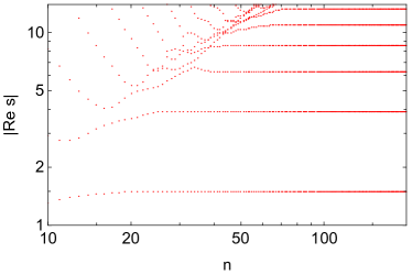
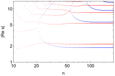
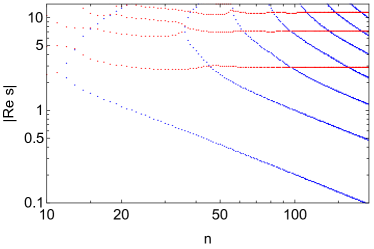
Figure 6: Convergence of real parts of oscillatory modes (red) and purely damped modes (blue) for $\lambda=1$, $l=0$, and $\sigma=0$ (left), $\sigma=0.5$ (right), or $\sigma=1$ (bottom) in case of the conformally invariant equation.

Figure 7 shows how real parts of the oscillatory modes and purely damped modes depend on $\sigma$. One can observe that at some point (for $\lambda=1$, $l=2$ it is $\sigma\approx 0.7$) the real part of the lowest decaying mode starts dominating over the lowest oscillatory mode. This transition is reflected in Fig. 5 by the emergence of the exponential tail. As $\sigma$ grows further, this tail decays. Finally, for $\sigma=1$ all the purely damped modes vanish (they converge to zero) and the tail is described by the power law. Dependence of the oscillatory modes frequencies on $\sigma$ is less severe and is presented in Fig. 8.

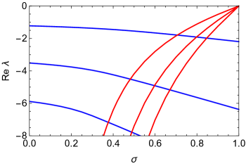
Figure 7: Variation with $\sigma$ of the real parts of three smallest oscillatory modes (blue) and purely damped modes (red) for conformally invariant equation with $\lambda=1$ and $l=2$.

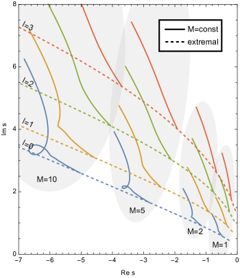
Figure 8: Oscillatory quasinormal frequencies for conformally invariant equation in Reissner-Nordström-anti-de Sitter spacetime with $\Lambda=-1$ and various masses $M$ and charges $Q$. The dashed lines indicate extremal cases. The solid lines bifurcating from them have constant mass $M$ and are parametrised by decreasing charge.

The same approach can be employed also to studies of perturbations of the spacetime. In a typical framework [9] they are described by the generalised eigenproblem

$$L\psi=V\psi,$$

where $V$ is the suitable spherically symmetric potential, depending on the type of the perturbations one studies (for its form in case of the RNAdS spacetime see [3]), and

$$L=\frac{d^{2}}{dr^{2}_{\ast}}+s^{2}.$$

By $r_{\ast}$ we denote here the tortoise coordinate that for metric (8) with $r_{H}=1$ can be defined by

$$\frac{d\rho}{dr_{\ast}}=f(\rho).$$

This eigenproblem can be obtained from the dynamical equation $\Box\psi+U\psi=0$, where $\Box$ is a wave operator for the metric (8) with $r_{H}=1$ in $(t_{H},\rho,\theta,\phi)$ coordinates and

$$U(\rho)=\left[\frac{f^{\prime}(\rho)}{\rho}+\frac{l(l+1)}{\rho^{2}}-\frac{V}{f(\rho)}\right].$$

The equation $\Box\psi+U\psi=0$ can be easily written in coordinates $(\tau,x,\theta,\phi)$. Hence, let us consider a wave equation with a general potential $U$:

$$\Box_{g}\psi+U\psi=0,$$ (13)

with $g$ denoting metric (11). As we have already pointed out, the wave operator $\Box_{g}$ contains a non-zero $\partial_{\tau}$ derivative term. Before we were able to get rid of it using the conformal invariance, however, for general potential $U$ equation (13) does not possess this feature. Luckily, in $3+1$ dimensions the wave operator has a useful property that under the conformal transformation $\tilde{g}=\Omega^{2}g$, $\tilde{\psi}=\Omega^{-1}\psi$ it behaves like [36]

$$\Box_{\tilde{g}}\tilde{\psi}=\Omega^{-3}\Box_{g}\psi-\Omega^{-4}(\Box_{g}\Omega)\psi.$$

As a result, we can use the same factor $\Omega$ as for the conformally invariant equation to get rid of the $\partial_{\tau}\psi$ term and the resulting operator will be the same differential operator plus an additional potential term. It leads us to the equivalent wave equation

$$\Box_{\tilde{g}}\tilde{\psi}+\left[\Omega^{-3}(\Box_{g}\Omega)+\Omega^{-2}U\right]\tilde{\psi}=0.$$ (14)

This equation is no longer regular since $\Omega^{-3}(\Box_{g}\Omega)$ behaves like $(1-x)^{-2}$ near $x=1$. However, it does not pose any problem since we are interested in solutions that satisfy Dirichlet condition at this end. Assuming that the solution vanishes at $x=1$ at least linearly together with an additional factor coming from the conformal transformation makes sure that the considered problem is sufficiently regular.

Equation (14) can be studied for the whole range of charges up to the extremal case with the same methods as discussed before. As an example, in Fig. (9) we show real and imaginary parts of the lowest quasinormal frequencies of the scalar (with $l=0$) and axial (with $l=2$) perturbations. These results regard spacetime with the AdS radius $\ell=1$, and various masses and charges set in such a way that the event horizon is localised at $r_{H}=5$. The plots are parametrised by the ratio of the charge $Q$ and the extremal charge $Q_{ext}=10\sqrt{19}$ in this setting (in the extremal case $M_{ext}=255$). It lets us compare the results of our approach with the previous results from [3], where the authors were considering an analogous problem for $Q\leq 0.55\,Q_{ext}$, and we find good agreement in this range.

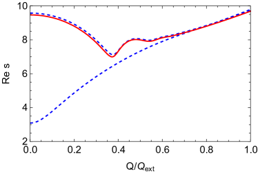
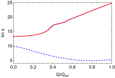
Figure 9: Quasinormal frequencies for perturbations of Reissner-Nordström-anti-de Sitter spacetime with $\ell=1$ and $r_{H}=5$. The solid red line denotes scalar perturbations with $l=0$ while blue dashed lines shows results for axial perturbations with $l=2$.

References

- [1] R. Abbott, et al. [LIGO Scientific and Virgo], Tests of general relativity with binary black holes from the second LIGO-Virgo gravitational-wave transient catalog, Phys. Rev. D 103 (2021), 122002.
- [2] W. Basel, Formal power series and linear systems of meromorphic ordinary differential equations, Springer (2000).
- [3] E. Berti and K. D. Kokkotas, Quasinormal modes of Reissner–Nordström–anti-de Sitter black holes: Scalar, electromagnetic, and gravitational perturbations, Phys. Rev. D 67 (2003), 064020.
- [4] E. Berti, V. Cardoso, J. A. Gonzalez, U. Sperhake, M. Hannam, S. Husa, and B. Bruegmann, Inspiral, merger and ringdown of unequal mass black hole binaries: A Multipolar analysis, Phys. Rev. D 76 (2007), 064034.
- [5] E. Berti, V. Cardoso, and A. O. Starinets, Quasinormal modes of black holes and black branes, Class. Quant. Grav. 26 (2009), 163001.
- [6] P. Bizoń, T. Chmaj, and P. Mach, A toy model of hyperboloidal approach to quasinormal modes, Acta Phys. Polon. B 51 (2020), 1007.
- [7] J.-F. Bony and D. Häfner, Decay and Non-Decay of the Local Energy for the Wave Equation on the De Sitter–Schwarzschild Metric, Commun. Math. Phys. 282 (2008), pp. 697–719.
- [8] A. Buonanno, G. B. Cook, and F. Pretorius, Inspiral, merger and ring-down of equal-mass black-hole binaries, Phys. Rev. D 75 (2007), 124018.
- [9] S. Chandrasekhar, The Mathematical Theory of Black Holes, Oxford University (1983).
- [10] S. L. Detweiler, Black holes and gravitational waves. III. The resonant frequencies of rotating holes, Astrophys. J. 239 (1980), pp. 292–295.
- [11] S. Dyatlov, Quasi-normal modes and exponential energy decay for the Kerr-de Sitter black hole, Commun. Math. Phys. 306 (2011), pp. 119–163.
- [12] S. Dyatlov and M. Zworski, Mathematical Theory of Scattering Resonances, vol. 200. American Mathematical Society (2019).
- [13] D. Gajic and C. Warnick, A model problem for quasinormal ringdown of asymptotically flat or extremal black holes, J. Math. Phys. 61 (2020), 102501.
- [14] D. Gajic and C. Warnick, Quasinormal Modes in Extremal Reissner-Nordström Spacetimes, Commun. Math. Phys. 385 (2021), pp. 1395–1498.
- [15] J. Galkowski and M. Zworski, Outgoing Solutions Via Gevrey-2 Properties, Ann. PDE 7, 5 (2021).
- [16] J. Galkowski and M. Zworski, Analytic hypoellipticity of Keldysh operators, Proc. London Math. Soc. 123 (2021), pp. 498–516.
- [17] O. Gannot, Existence of Quasinormal Modes for Kerr-AdS Black Holes, Annales Henri Poincare 18 (2017), pp. 2757-2788.
- [18] P. Hintz and Y. Xie, Quasinormal modes of small Schwarzschild-de Sitter black holes, J. Math. Phys. 63 (2022), 011509.
- [19] P. Hintz, Mode stability and shallow quasinormal modes of Kerr-de Sitter black holes away from extremality, arXiv:2112.14431 [gr-qc].
- [20] S. Hod, Quasinormal resonances of near-extremal Kerr-Newman black holes, Phys. Lett. B 666 (2008), pp. 483–485.
- [21] S. Hod, Slow relaxation of rapidly rotating black holes, Phys. Rev. D 78 (2008), 084035.
- [22] S. Hod, Black-hole quasinormal resonances: Wave analysis versus a geometric-optics approximation, Phys. Rev. D 80 (2009), 064004.
- [23] S. Hod, Relaxation dynamics of charged gravitational collapse, Phys. Lett. A 374 (2010), 2901.
- [24] S. Hod, Quasinormal resonances of a massive scalar field in a near-extremal Kerr black hole spacetime, Phys. Rev. D 84 (2011), 044046.
- [25] S. Hod, Quasinormal resonances of a charged scalar field in a charged Reissner-Nordstroem black-hole spacetime: A WKB analysis, Phys. Lett. B 710 (2012), pp. 349–351.
- [26] J. Joykutty, Existence of Zero-Damped Quasinormal Frequencies for Nearly Extremal Black Holes, Annales Henri Poincare 23 (2022), pp. 4343–4390.
- [27] K. D. Kokkotas and B. G. Schmidt, Quasinormal modes of stars and black holes, Living Rev. Rel. 2 (1999), 2.
- [28] R. Konoplya and A. Zhidenko, Quasinormal modes of black holes: From astrophysics to string theory, Rev. Mod. Phys. 83 (2011), pp. 793–836.
- [29] E. W. Leaver, An analytic representation for the quasi-normal modes of Kerr black holes, Proc. R. Soc. A 402 (1985), pp. 285–298.
- [30] E. W. Leaver, Quasinormal modes of Reissner-Nordström black holes, Phys. Rev. D 41 (1990), 2986.
- [31] O. Petersen and A. Vasy, Stationarity and Fredholm theory in subextremal Kerr-de Sitter spacetimes, arXiv:2306.09213 [math.AP].
- [32] O. Petersen, A. Vasy, Analyticity of Quasinormal Modes in the Kerr and Kerr–de Sitter Spacetimes, Commun. Math. Phys. 402 (2023), pp. 2547–2575.
- [33] A. Sá Barreto and M. Zworski, Distribution of resonances for spherical black holes, Mathematical Research Letters 4 (1997), pp. 103–121.
- [34] B. G. Schmidt, On relativistic stellar oscillations, Gravity Research Foundation essay (1993).
- [35] A. Vasy, Microlocal analysis of asymptotically hyperbolic and Kerr-de Sitter spaces (with an appendix by Semyon Dyatlov), Inventiones mathematicae 194 (2013), pp. 381–513.
- [36] R. Wald, General Relativity, The University of Chicago Press (1984).
- [37] C. M. Warnick, On quasinormal modes of asymptotically anti-de Sitter black holes, Commun. Math. Phys. 333 (2015), pp. 959–1035.
- [38] G. N. Watson, A treatise on the theory of Bessel Functions, CUP (1922).
- [39] H. Yang, A. Zimmerman, A. Zenginoğlu, F. Zhang, E. Berti, and Y. Chen, Quasinormal modes of nearly extremal Kerr spacetimes: spectrum bifurcation and power-law ringdown, Phys. Rev. D 88 (2013), 044047.
- [40] A. Zimmerman and Z. Mark, Damped and zero-damped quasinormal modes of charged, nearly extremal black holes, Phys. Rev. D 93 (2016), 044033.
- [41] P. Zimmerman, Horizon instability of extremal Reissner-Nordström black holes to charged perturbations, Phys. Rev. D 95 (2017), 124032.