Finding-Aware Anatomical Tokens for Chest X-Ray Automated Reporting

Abstract

The task of radiology reporting comprises describing and interpreting the medical findings in radiographic images, including description of their location and appearance. Automated approaches to radiology reporting require the image to be encoded into a suitable token representation for input to the language model. Previous methods commonly use convolutional neural networks to encode an image into a series of image-level feature map representations. However, the generated reports often exhibit realistic style but imperfect accuracy. Inspired by recent works for image captioning in the general domain in which each visual token corresponds to an object detected in an image, we investigate whether using local tokens corresponding to anatomical structures can improve the quality of the generated reports. We introduce a novel adaptation of Faster R-CNN in which finding detection is performed for the candidate bounding boxes extracted during anatomical structure localisation. We use the resulting bounding box feature representations as our set of finding-aware anatomical tokens. This encourages the extracted anatomical tokens to be informative about the findings they contain (required for the final task of radiology reporting). Evaluating on the MIMIC-CXR dataset [16, 17, 12] of chest X-Ray images, we show that task-aware anatomical tokens give state-of-the-art performance when integrated into an automated reporting pipeline, yielding generated reports with improved clinical accuracy.

1 Introduction

A radiology report is a detailed text description and interpretation of the findings in a medical scan, including description of their anatomical location and appearance. For example, a Chest X-Ray (CXR) report may describe an opacity (a type of finding) in the left upper lung (the relevant anatomical location) which is diagnosed as a lung nodule (interpretation). The combination of a finding and its anatomical location influences both the diagnosis and the clinical treatment decision, since the same finding may have a different list of possible clinical diagnoses depending on the location.

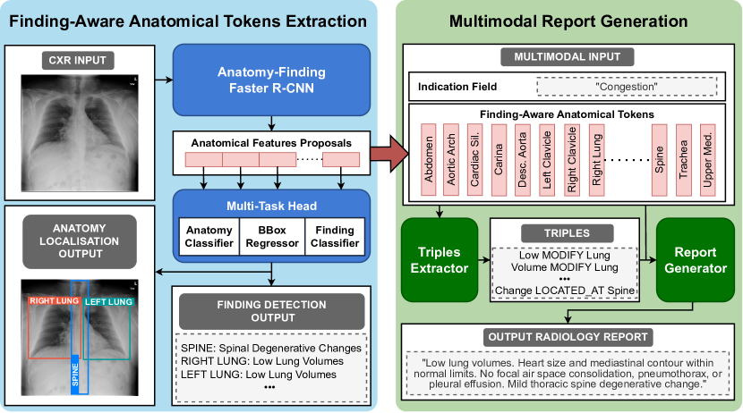
Figure 1: Finding-aware anatomical tokens integrated into a multimodal CXR automated reporting pipeline. The CXR image and report are taken from the IU-Xray dataset [7].

Recent CXR automated reporting methods have adopted CNN-Transformer architectures, in which the CXR is encoded using Convolutional Neural Networks (CNNs) into global image-level features [13, 14] which are input to a Transformer language model [32] to generate the radiology report. However, the generated reports often exhibit realistic style but imperfect accuracy, for instance hallucinating additional findings or describing abnormal regions as normal. Inspired by recent image captioning works in the general domain [2, 19, 37] in which each visual token corresponds to an object detected in the input image, we investigate whether replacing the image-level tokens with local tokens – corresponding to anatomical structures – can improve the clinical accuracy of the generated reports. Our contributions are to:

1. Propose a novel multi-task Faster R-CNN [27] to extract finding-aware anatomical tokens by performing finding detection on the candidate bounding boxes identified during anatomical structure localisation. We ensure these tokens convey rich information by training the model on an extensive set of anatomy regions and associated findings from the Chest ImaGenome dataset [34, 12].

2. Integrate the extracted finding-aware anatomical tokens as the visual input in a state-of-the-art two-stage pipeline for radiology report generation [6]; this pipeline is multimodal, taking both image (CXR) and text (the corresponding text indication field) as inputs.

3. Demonstrate the benefit of using these tokens for CXR report generation through in-depth experiments on the MIMIC-CXR dataset.

2 Related Works

Automated Reporting

Previous works on CXR automated reporting have examined the model architecture [5, 4], the use of additional loss functions [24], retrieval-based report generation [29, 10], and grounding report generation with structured knowledge [6, 35]. However, no specific focus has been given to the image encoding. Inspired by recent works in image captioning in the general domain [2, 19, 37], where each visual token corresponds to an object detected in an image, we propose to replace the image-level representations with local representations corresponding to anatomical structures detected in a CXR. To the best of our knowledge, only [33, 30] have considered anatomical feature representations for CXR automated reporting. In [33], they extract anatomical features from an object detection model trained solely on the anatomy localisation task. In [30], they train the object detector through multiple steps – anatomy localisation, binary abnormality classification and region selection – and feed each anatomical region individually to the language model to generate one sentence at a time. This approach makes the simplistic assumption that one anatomical region is described in exactly one report sentence.

Finding Detection

Prior works have tackled the problem of finding detection in CXR images via weakly supervised approaches [36, 38]. However, the design of these approaches does not allow the extraction of anatomy-specific vector representations, making them unsuited for our purpose. Agu et al [1] proposed AnaXnet, comprising two modules trained independently: a standard Faster R-CNN trained to localise anatomical regions, and a Graph Convolutional Network (GCN) trained to classify the pathologies appearing in each anatomical region bounding box. This approach assumes that the finding information is present in the anatomical representations after the first stage of training.

3 Methods

We describe our method in two parts: (1) Finding-aware anatomical token extraction (Figure 1, left) – a custom Faster R-CNN which is trained to jointly perform anatomy localisation and finding detection; and (2) Multimodal report generation (Figure 1, right) – a two-step pipeline which is adapted to perform triples extraction and report generation, using the anatomical tokens extracted from the Faster R-CNN as the visual inputs for the multimodal Transformer backbone [32].

3.1 Finding-Aware Anatomical Token Extraction

Let us consider $A=\{a_{n}\}_{n=1}^{N}$ as the set of anatomical regions in a CXR and $F=\{f_{m}\}_{m=1}^{M}$ the set of findings we aim to detect. We define $f_{n,m}\in\{0,1\}$ indicating the absence or presence of the finding $f_{m}$ in the anatomical region $a_{n}$, and $f_{n}=\{f_{n,m}\}_{m=1}^{M}$ as the set of findings in $a_{n}$. We define anatomy localisation as the task of predicting the top-left and bottom-right bounding box coordinates $c=(c_{x1},c_{y1},c_{x2},c_{y2})$ of the anatomical regions $A$; and finding detection as the task of predicting the findings $f_{n}$ at each location $a_{n}$.

We frame anatomy localisation as a general object detection task, employing the Faster R-CNN framework to compute the coordinates of the bounding boxes and the anatomical labels assigned to each of them. First, the image features are extracted from the CNN backbone, composed of a ResNet-50 [13] and a Feature Pyramid Network (FPN) [22]. Second, the multi-scale image features extracted from the FPN are passed to the Region Proposal Network (RPN) to generate the bounding box coordinates $c_{k}=(c_{k,x1},c_{k,y1},c_{k,x2},c_{k,y2})$ for each proposal $k$ and to the Region of Interest (RoI) pooling layer, designed to extract the respective fixed-length vector representation $l_{k}\in\mathbb{R}^{1024}$. Each proposal’s local features $l_{k}$ are then passed to a classification layer (Anatomy Classifier) to assign the anatomical label ($a_{k}$) and to a bounding box regressor layer to refine the coordinates. In parallel, we insert a multi-label classification head (Findings Classifier) – consisting of a single fully-connected layer with sigmoid activation functions – that classifies a set of findings for each proposal’s local features (see Appendix 0.A).

During training, we use a multi-task loss comprising three terms: anatomy classification loss, box regression loss, and (multi-label) finding classification loss. Formally, for each predicted bounding box, this is computed as

$$\mathcal{L}=\mathcal{L}_{anatomy}+\mathcal{L}_{box}+\lambda\mathcal{L}_{finding},$$ (1)

where $\mathcal{L}_{anatomy}$ and $\mathcal{L}_{box}$ correspond to the anatomy classification loss and the bounding box regression loss described in [11] and ${L}_{finding}$ is the finding classification loss that we introduce; $\lambda$ is a balancing hyper-parameter set to $\lambda=10^{2}$. We define

$$\mathcal{L}_{finding}=-\sum_{k=1}^{K}\sum_{m=1}^{M}w_{m}f_{k,m}\log(p_{k,m})$$ (2)

a binary cross-entropy loss between the predicted probability $p_{k}=\{p_{k,m}\}_{m=1}^{M}$ of the $k$-th proposal and its associated ground truth $f_{k}=\{f_{k,m}\}_{m=1}^{M}$ (with $f_{k}=f_{m}$ if $a_{k}=a_{m}$). We class weight using $w_{m}=(1/\nu_{m})^{\alpha}$, where $\nu_{m}$ is the frequency of the finding $f_{m}$ in the training dataset and we empirically set $\alpha$ to 0.25.

At inference time, for each CXR image, we extract the finding-aware anatomical tokens $A_{tok}=\{l_{n}\}_{n=1}^{N}$, by selecting for each anatomical region the proposal with highest anatomical classification score and taking the associated latent vector representation $l_{n}$. Any non-detected regions are assigned a $1024$-dimensional vector of zeros. $A_{tok}$ is provided as input to the report generation model.

3.2 Multimodal Report Generation

We adopt the multimodal knowledge-grounded approach for automated reporting on CXR images as proposed in [6]. Firstly, triples extraction is performed to extract structured information from a CXR image in the form of triples, given the indication field $Ind$ as context. Secondly, report generation is performed to generate the radiology report from the triples with the CXR image and indication field again provided as context.

Each step is treated as a sequence-to-sequence task; for this purpose, the triples are concatenated into a single text sequence (in the order they appear in the ground truth report) separated by the special [SEP] token to form $Trp$, and the visual tokens are concatenated in a fixed order of anatomical regions. Two multimodal encoder-decoder Transformers are employed as the Triples Extractor ($TE$) and Report Generator ($RG$). The overall approach is:

Step 1 $$\quad\quad\quad Trp=TE(seg_{1}=A_{tok},seg_{2}=Ind)$$ (3)

Step 2 $$\quad\quad\quad R=RG(seg_{1}=A_{tok},seg_{2}=Ind\texttt{ [SEP] }Trp)$$

where $seg_{1}$ and $seg_{2}$ are the two input segments which are themselves concatenated at the input. In step 2, the indication field and the triples are merged into a single sequence of text by concatenating them, separated by the special [SEP] token. Similarly to [8], the input to a Transformer corresponds to the sum of the textual and visual token embeddings, the positional embeddings—to inform about the order of the tokens—and the segment embeddings—to discriminate between the two modalities.

4 Experimental Setup

4.1 Datasets and Metrics

We base our experiments on two open-source CXR imaging datasets, Chest ImaGenome [34, 12] and MIMIC-CXR [16, 17, 12]. The MIMIC-CXR dataset comprises CXR image-report pairs and is used for the target task of report generation. The Chest ImaGenome dataset is derived from MIMIC-CXR, extended with additional automatically extracted annotations for 242,072 anteroposterior and posteroanterior CXR images, which we use to train the finding-aware anatomical token extractor. We follow the same train/validation/test split as proposed in the Chest ImaGenome dataset. We extract the Findings section of each report as the target text. For the textual input, we extract the Indication field from each report. We annotate the ground truth triples for each image-report pair following a semi-automated pipeline using RadGraph [15] and sciSpaCy [25], as described in [6].

To assess the quality of the generated reports, we compute Natural Language Generation (NLG) metrics: BLEU [26], ROUGE [21] and METEOR [3]. We further compute Clinical Efficiency (CE) metrics by applying the CheXbert labeller [28] which extracts 14 findings to the ground truth and the generated reports, and evaluate F1, precision and recall scores. We repeat each experiment 3 times using different random seeds, reporting the average in our results.

4.2 Implementation

Finding-aware anatomical token extractor:

We adapt the Faster R-CNN implementation from [20], by including the finding classifier. We initialise the network with weights pre-trained on the COCO dataset [23], then fine-tune it to localise 36 anatomical regions and to detect 71 findings within each region, as annotated in the Chest ImaGenome dataset (see Appendix 0.C). The CXR images are resized by matching the shorter dimension to 512 pixels (maintaining the original aspect ratio) and cropping to a resolution of $512\times 512$ (random crop during training and centre crop during inference). We train the model for 25 epochs with a learning rate of $10^{-3}$, decayed every 5 epochs by a factor of 0.8. We select the model with the highest finding detection performances for the validation set, measured by computing the AUROC score for each finding at each anatomical region (see results in Appendix 0.B).

Report generator:

We implement a vanilla Transformer encoder-decoder at each step of the automated reporting pipeline. Both the encoder and the decoder consist of 3 attention layers, each composed of 8 heads and 512 hidden units. All the parameters are randomly initialised. We train step 1 for 40 epochs, with the learning rate set to $10^{-4}$ and we decay it by a factor of 0.8 every 3 epochs; and step 2 for 20 epochs, with the same learning rate as step 1. During training, we follow [6] in masking out a proportion of the ground-truth triples (50%, determined empirically), while during inference we use the triples extracted at step 1. We select the model with the highest CE-F1 score on the validation set.

Baselines

We benchmark against other CXR automated reporting methods: R2Gen [5], R2GenCMN [4], $\mathcal{M}^{2}$ Tr.+fact${}_{\text{ENTNLI}}$ [24], CNN+Two-Step [6] and RGRG [30]. All these methods (except RGRG) adopt a CNN-Transformer and have shown state-of-the-art performances in report generation on the MIMIC-CXR dataset. All reported values are re-computed using the original code based on the same data split and image resolution as our method, except for [30] who already used this data split and image resolution, therefore we cite their reported results. We keep remaining hyperparameters as the originally reported values.

5 Results

Overall results

In Table 1, we benchmark against other state-of-the-art CXR automated reporting methods and compare with the $A_{tok}$ integrated into the full pipeline versus a simpler approach of the report generator model only, $RG$, which generates the report directly from image and indication field (omitting triples extraction). The proposed finding-aware anatomical tokens integrated with a knowledge-grounded pipeline [6] generate reports with state-of-the-art fluency (NLG metrics) and clinical accuracy (CE metrics). Moreover, the superior results of our $A_{tok}$ + RG approach compared to RGRG [30] suggests that providing the full set of anatomical tokens together, instead of separately, gives better results. The broader visual context is indeed necessary when describing findings that span multiple regions e.g., assessing the position of a tube.

Table 1: Comparison of our proposed solution with previous approaches. TE = Triples Extractor, RG = Report Generator.

Method	NLG						CE
	BL-1	BL-2	BL-3	BL-4	MTR	RG-L	F1	P	R
R2Gen [5]	0.381	0.248	0.174	0.130	0.152	0.314	0.431	0.511	0.395
R2GenCMN [4]	0.365	0.239	0.169	0.126	0.145	0.309	0.371	0.462	0.311
$\mathcal{M}^{2}$ Tr. + fact${}_{\text{ENTNLI}}$ [24]	0.402	0.261	0.183	0.136	0.158	0.300	0.458	0.540	0.404
ResNet-101 + $TE$ + $RG$ [6]	0.468	0.343	0.271	0.223	0.200	0.390	0.477	0.556	0.418
RGRG [30]	0.400	0.266	0.187	0.135	0.168	-	0.461	0.475	0.447
$A_{tok}$ + $RG$ (ours)	0.422	0.324	0.265	0.225	0.201	0.426	0.515	0.579	0.464
$A_{tok}$ + $TE$ + $RG$ (ours)	0.490	0.363	0.288	0.237	0.213	0.406	0.537	0.585	0.496

Table 2: Comparison of different visual input representations (ResNet-101 vs. $A_{tok}$) using different pre-training supervision (ImageNet, Findings, Anatomy and Anatomy+Findings), integrated with the TE+RG two-step pipeline.

Visual	Supervision	NLG						CE
Input		BL-1	BL-2	BL-3	BL-4	MTR	RG-L	F1	P	R
ResNet-101	ImageNet	0.468	0.343	0.271	0.223	0.200	0.390	0.477	0.556	0.418
ResNet-101	Findings	0.472	0.346	0.273	0.225	0.202	0.396	0.495	0.565	0.440
Naive $A_{tok}$	Anatomy	0.436	0.320	0.253	0.208	0.187	0.387	0.392	0.487	0.329
$A_{tok}$	Anatomy+Findings	0.490	0.363	0.288	0.237	0.213	0.406	0.537	0.585	0.496

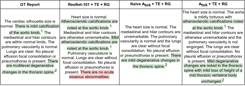
Figure 2: Example report generated with different visual representations. The ground truth (GT) report (left) is followed by the generated reports using ResNet-101, naive anatomical tokens, and finding-aware anatomical tokens. Correctly detected findings are coloured green and errors are coloured red; we number corresponding descriptions.

Ablation Study

Table 2 shows the results of adopting different visual representations. Firstly, we use a CNN (ResNet-101) trained end-to-end with $TE$+$RG$ and initialised two ways: pre-trained on ImageNet versus pretrained on the Findings labels of Chest ImaGenome (details provided in Appendix 0.D). Secondly, we extract anatomical tokens (A_tok) with different supervision of Faster R-CNN: anatomy localisation only (Anatomy) or anatomy localisation + finding detection (Anatomy+Findings). The results show the positive effect of including supervision with finding detection either when pre-training ResNet-101 or as an additional task for Faster R-CNN. Example reports are shown in Figure 2 (abbreviated) and Appendix 0.F (extended).

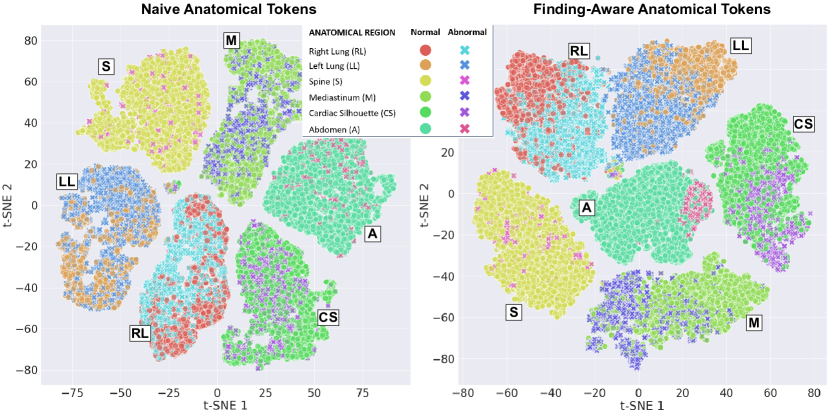
Figure 3: T-SNE visualisation of normal and abnormal embeddings for a subset of visual tokens. Left: naive anatomical token embeddings extracted from Faster R-CNN trained solely on anatomy localisation. Right: task-aware anatomical token embeddings extracted from Faster R-CNN trained also on the finding detection task.

Anatomical Embedding Distributions

In Figure 3, we visualise the impact of the finding detection task on the extracted anatomical tokens. To generate these plots, for 3000 randomly selected test set scans, we first perform principle component analysis [18] for dimensionality reduction of the token embeddings (from $\mathbb{R}^{1024}$ to $\mathbb{R}^{50}$), then use t-distributed stochastic neighbour embedding (t-SNE) [31], colour coding the extracted embeddings by their anatomical region and additionally categorising as normal or abnormal (a token is considered abnormal if at least one of the 71 findings is positively labeled). For most anatomical regions, the normal and abnormal groups are better separated by the finding-aware tokens, suggesting these tokens successfully transmit information about findings. We also compute the mean distance between normal and abnormal clusters using Fréchet Distance (mFD) [9], measuring mFD=8.80 (naive anatomical tokens) and mFD=78.67 (finding-aware anatomical tokens).

6 Conclusion

This work explores how to extract and integrate anatomical visual representations with language models, targeting the task of automated radiology reporting. We propose a novel multi-task Faster R-CNN adaptation that performs finding detection jointly with anatomy localisation, to extract finding-aware anatomical tokens. We then integrate these tokens as the visual input for a multimodal image+text report generation pipeline, showing that finding-aware anatomical tokens improve the fluency (NLG metrics) and clinical accuracy (CE metrics) of the generated reports, giving state-of-the-art results.

Supplementary Material

Appendix 0.A Anatomy-Finding Faster R-CNN Architecture

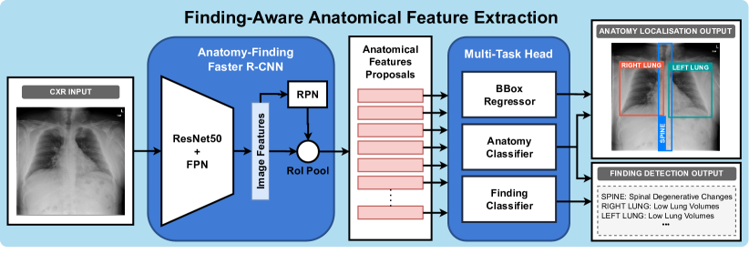
Figure 4: The proposed anatomy-finding Faster R-CNN trained jointly on anatomy localisation and finding detection.

Appendix 0.B Anatomy Localisation & Finding Detection Results

Table 3: Anatomy localisation and finding detection results of different configurations of the proposed Faster R-CNN: anatomy localisation only (Anatomy); and including the finding classification head (Finding) (our proposed solution).

Supervision		Anatomy Localisation	Finding Detection
Anatomy	Finding	mAP@0.5	AUROC
✓		0.938	-
✓	✓	0.918	0.863

We evaluate the anatomy localisation performance of our proposed Faster R-CNN by computing the mean Average Precision (mAP@0.5), with positive detections when the Intersection over Union score between the predicted bounding boxes and the ground truth is above 0.5. Finding detection performance is measured by computing the Area Under the Receiver Operating Characteristic (AUROC) for each finding at each anatomical region.

Table 3 shows that our proposed anatomy-finding Faster R-CNN performs worse than a standard Faster R-CNN trained solely on anatomy localisation in terms of mAP@0.5 while achieving a good finding detection score. This is expected, as we select the best anatomy-only Faster R-CNN model based on the highest mAP@0.5 on the validation set and the anatomy-finding Faster R-CNN model based on the finding detection AUROC score. We observe that the trade-off between anatomy localisation and finding detection performance can be tuned by adjusting the weighting hyperparameter $\lambda$ in the multi-task loss.

Appendix 0.C Anatomical Regions & Findings

Table 4: Complete set of 36 anatomical regions and 71 findings used to supervise the anatomy localisation and the finding detection tasks, as annotated in the Chest ImaGenome dataset (https://physionet.org/content/chest-imagenome/1.0.0/).

Anatomical Regions
abdomen	left clavicle	mediastinum	right lower lung zone
aortic arch	left costophrenic angle	right apical zone	right lung
cardiac silhouette	left hemidiaphragm	right atrium	right mid lung zone
carina	left hilar structures	right cardiac silhouette	right upper abdomen
cavoatrial junction	left lower lung zone	right cardiophrenic angle	right upper lung zone
descending aorta	left lung	right clavicle	spine
left apical zone	left mid lung zone	right costophrenic angle	svc
left cardiac silhouette	left upper abdomen	right hemidiaphragm	trachea
left cardiophrenic angle	left upper lung zone	right hilar structures	upper mediastinum
Findings
airspace opacity	cyst/bullae	linear/patchy atelectasis	pneumothorax
alveolar hemorrhage	diaphragmatic eventration (benign)	lobar/segmental collapse	prosthetic valve
aortic graft/repair	elevated hemidiaphragm	low lung volumes	pulmonary edema/hazy opacity
artifact	endotracheal tube	lung cancer	rotated
aspiration	enlarged cardiac silhouette	lung lesion	scoliosis
atelectasis	enlarged hilum	lung opacity	shoulder osteoarthritis
bone lesion	enteric tube	mass/nodule (not otherwise specified)	spinal degenerative changes
breast/nipple shadows	fluid overload/heart failure	mediastinal displacement	spinal fracture
bronchiectasis	goiter	mediastinal drain	sub-diaphragmatic air
cabg grafts	granulomatous disease	mediastinal widening	subclavian line
calcified nodule	hernia	multiple masses/nodules	superior mediastinal mass/enlargement
cardiac pacer and wires	hydropneumothorax	pericardial effusion	swan-ganz catheter
chest port	hyperaeration	picc	tortuous aorta
chest tube	ij line	pigtail catheter	tracheostomy tube
clavicle fracture	increased reticular markings/ild pattern	pleural effusion	vascular calcification
consolidation	infiltration	pleural/parenchymal scarring	vascular congestion
copd/emphysema	interstitial lung disease	pneumomediastinum	vascular redistribution
costophrenic angle blunting	intra-aortic balloon pump	pneumonia

Appendix 0.D CNN Pre-Training on Chest ImaGenome Findings

We train ResNet-101 on the set of 71 findings labels listed in Appendix 0.C. Differently from Faster R-CNN, ResNet-101 is trained only to classify whether findings are present or absent in a CXR without any further anatomical localisation of each finding. We train ResNet-101 for 50 epochs, with an initial learning rate set to $10^{-3}$ and decrease every 2 epochs by a factor of $0.5$. The loss term corresponds to a binary cross-entropy:

$$\mathcal{L}_{class}=-\sum_{m=1}^{M}w_{m}f_{m}\log(p_{m})$$

between the predicted probability of each class $p_{m}$ and the ground truth $f_{m}$. We class weight with $w_{m}=(1/\nu_{m})^{0.25}$, where $\nu_{m}$ corresponds to the frequency of the finding $f_{m}$ in the training set.

Appendix 0.E Hyperparameter Search

Table 5: Hyperparameter search space. We highlight in bold the chosen values.

Model	Hyperparameter	Search Space
Anatomy-Finding Faster R-CNN	learning rate	{0.001, 0.0005, 0.0001, 0.00005}
	$\lambda$	{1, 10, 100, 1000}
	$\alpha$	{0, 0.25, 0.50, 0.75, 1}
Triples Extractor	learning rate	{0.0005, 0.0001, 0.00005}
Report Generator	learning rate	{0.0005, 0.0001, 0.00005}
	triples masking %	{30, 40, 50, 60, 70}

Appendix 0.F Example predicted reports

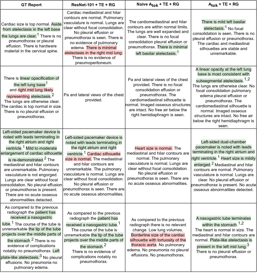
Figure 5: Examples of predicted reports with different visual representations (examples selected randomly from the subset of reports where predictions were different between representation methods). From left to right: the ground truth (GT) report, the predicted reports using a CNN, the naive anatomical tokens and the finding-aware anatomical tokens as the visual representations. In generated reports, correctly detected positive findings are highlighted in green, and errors are highlighted in red. The equivalent text spans in the ground truth report are also highlighted; we number corresponding descriptions.

References

- [1] Nkechinyere N Agu, Joy T Wu, Hanqing Chao, Ismini Lourentzou, Arjun Sharma, Mehdi Moradi, Pingkun Yan and James Hendler “AnaXNet: Anatomy Aware Multi-label Finding Classification in Chest X-Ray” In MICCAI, 2021 Springer
- [2] Peter Anderson, Xiaodong He, Chris Buehler, Damien Teney, Mark Johnson, Stephen Gould and Lei Zhang “Bottom-Up and Top-Down Attention for Image Captioning and Visual Question Answering” In CVPR, 2018
- [3] Satanjeev Banerjee and Alon Lavie “METEOR: An automatic metric for MT evaluation with improved correlation with human judgments” In ACL Workshop on Intrinsic and Extrinsic Evaluation Measures for Machine Translation and/or Summarization, 2005, pp. 65–72
- [4] Zhihong Chen, Yaling Shen, Yan Song and Xiang Wan “Cross-modal Memory Networks for Radiology Report Generation” In ACL-IJCNLP, 2021, pp. 5904–5914
- [5] Zhihong Chen, Yan Song, Tsung-Hui Chang and Xiang Wan “Generating Radiology Reports via Memory-driven Transformer” In EMNLP, 2020, pp. 1439–1449
- [6] Francesco Dalla Serra, William Clackett, Hamish MacKinnon, Chaoyang Wang, Fani Deligianni, Jeff Dalton and Alison Q O’Neil “Multimodal Generation of Radiology Reports using Knowledge-Grounded Extraction of Entities and Relations” In AACL-IJCNLP, 2022, pp. 615–624
- [7] Dina Demner-Fushman, Marc D. Kohli, Marc B. Rosenman, Sonya E. Shooshan, Laritza M. Rodriguez, S. Antani, George R. Thoma and Clement J. McDonald “Preparing a collection of radiology examinations for distribution and retrieval” In JAMIA 23 2, 2016, pp. 304–10
- [8] Jacob Devlin, Ming-Wei Chang, Kenton Lee and Kristina Toutanova “BERT: Pre-training of Deep Bidirectional Transformers for Language Understanding” In NAACL Association for Computational Linguistics, 2019, pp. 4171–4186
- [9] DC Dowson and BV666017 Landau “The Fréchet distance between multivariate normal distributions” In JMA 12.3 Elsevier, 1982, pp. 450–455
- [10] Mark Endo, Rayan Krishnan, Viswesh Krishna, Andrew Y Ng and Pranav Rajpurkar “Retrieval-Based Chest X-Ray Report Generation Using a Pre-trained Contrastive Language-Image Model” In MLH, 2021, pp. 209–219 PMLR
- [11] Ross Girshick “Fast R-CNN” In ICCV, 2015, pp. 1440–1448
- [12] Ary L Goldberger et al. “PhysioBank, PhysioToolkit, and PhysioNet: components of a new research resource for complex physiologic signals” In circulation 101.23 Am Heart Assoc, 2000, pp. e215–e220
- [13] Kaiming He, Xiangyu Zhang, Shaoqing Ren and Jian Sun “Deep Residual Learning for Image Recognition” In CVPR, 2016, pp. 770–778
- [14] Gao Huang, Zhuang Liu, Laurens Van Der Maaten and Kilian Q Weinberger “Densely Connected Convolutional Networks” In CVPR, 2017, pp. 4700–4708
- [15] Saahil Jain et al. “RadGraph: Extracting Clinical Entities and Relations from Radiology Reports” In NeurIPS: Datasets and Benchmarks Track (Round 1), 2021
- [16] Alistair EW Johnson, Tom J Pollard, Seth J Berkowitz, Nathaniel R Greenbaum, Matthew P Lungren, Chih-ying Deng, Roger G Mark and Steven Horng “MIMIC-CXR, a de-identified publicly available database of chest radiographs with free-text reports” In Scientific Data 6.1 Springer ScienceBusiness Media LLC, 2019
- [17] Alistair EW Johnson et al. “MIMIC-CXR-JPG, a large publicly available database of labeled chest radiographs” In arXiv preprint arXiv:1901.07042, 2019
- [18] Ian Jolliffe “Principal component analysis” New York: Springer Verlag, 2002
- [19] Xiujun Li et al. “Oscar: Object-Semantics Aligned Pre-training for Vision-Language Tasks” In ECCV, 2020, pp. 121–137 Springer
- [20] Yanghao Li, Saining Xie, Xinlei Chen, Piotr Dollar, Kaiming He and Ross Girshick “Benchmarking Detection Transfer Learning with Vision Transformers” In arXiv preprint arXiv:2111.11429, 2021
- [21] Chin-Yew Lin “ROUGE: A Package for Automatic Evaluation of Summaries” In Text Summarization Branches Out, 2004, pp. 74–81
- [22] Tsung-Yi Lin, Piotr Dollár, Ross Girshick, Kaiming He, Bharath Hariharan and Serge Belongie “Feature pyramid networks for object detection” In CVPR, 2017, pp. 2117–2125
- [23] Tsung-Yi Lin, Michael Maire, Serge Belongie, James Hays, Pietro Perona, Deva Ramanan, Piotr Dollár and C Lawrence Zitnick “Microsoft COCO: common objects in context” In ECCV, 2014 Springer
- [24] Yasuhide Miura, Yuhao Zhang, Emily Tsai, Curtis Langlotz and Dan Jurafsky “Improving Factual Completeness and Consistency of Image-to-Text Radiology Report Generation” In NAACL, 2021, pp. 5288–5304
- [25] Mark Neumann, Daniel King, Iz Beltagy and Waleed Ammar “ScispaCy: Fast and Robust Models for Biomedical Natural Language Processing” In BioNLP Workshop and Shared Task, 2019, pp. 319–327
- [26] Kishore Papineni, Salim Roukos, Todd Ward and Wei-Jing Zhu “BLEU: a Method for Automatic Evaluation of Machine Translation” In ACL, 2002, pp. 311–318
- [27] Shaoqing Ren, Kaiming He, Ross Girshick and Jian Sun “Faster R-CNN: Towards real-time object detection with region proposal networks” In NIPS 28, 2015
- [28] Akshay Smit, Saahil Jain, Pranav Rajpurkar, Anuj Pareek, Andrew Y Ng and Matthew Lungren “Combining Automatic Labelers and Expert Annotations for Accurate Radiology Report Labeling Using BERT” In EMNLP, 2020, pp. 1500–1519
- [29] Tanveer Syeda-Mahmood et al. “Chest X-ray Report Generation through Fine-Grained Label Learning” In MICCAI, 2020, pp. 561–571 Springer
- [30] Tim Tanida, Philip Müller, Georgios Kaissis and Daniel Rueckert “Interactive and Explainable Region-guided Radiology Report Generation” In CVPR, 2023, pp. 7433–7442
- [31] Laurens Van der Maaten and Geoffrey Hinton “Visualizing data using t-SNE.” In JMLR 9.11, 2008
- [32] Ashish Vaswani, Noam Shazeer, Niki Parmar, Jakob Uszkoreit, Llion Jones, Aidan N Gomez, Łukasz Kaiser and Illia Polosukhin “Attention Is All You Need” In NIPS 30, 2017
- [33] Yuhao Wang, Kai Wang, Xiaohong Liu, Tianrun Gao, Jingyue Zhang and Guangyu Wang “Self adaptive global-local feature enhancement for radiology report generation” In arXiv preprint arXiv:2211.11380, 2022
- [34] Joy T Wu et al. “Chest ImaGenome Dataset for Clinical Reasoning” In NeurIPS: Datasets and Benchmarks Track (Round 2), 2021
- [35] Shuxin Yang, Xian Wu, Shen Ge, S Kevin Zhou and Li Xiao “Knowledge Matters: Chest Radiology Report Generation with General and Specific Knowledge” In MIA Elsevier, 2022, pp. 102510
- [36] Ke Yu, Shantanu Ghosh, Zhexiong Liu, Christopher Deible and Kayhan Batmanghelich “Anatomy-Guided Weakly-Supervised Abnormality Localization in Chest X-rays” In MICCAI, 2022 Springer
- [37] Pengchuan Zhang, Xiujun Li, Xiaowei Hu, Jianwei Yang, Lei Zhang, Lijuan Wang, Yejin Choi and Jianfeng Gao “VinVL: Revisiting Visual Representations in Vision-Language Models” In CVPR, 2021, pp. 5579–5588
- [38] Xiongfeng Zhu, Shumao Pang, Xiaoxuan Zhang, Junzhang Huang, Lei Zhao, Kai Tang and Qianjin Feng “PCAN: Pixel-wise classification and attention network for thoracic disease classification and weakly supervised localization” In CMIG 102 Elsevier, 2022, pp. 102137