Scalable Estimation of Probit Models with Crossed Random Effects

Abstract

Crossed random effects structures arise in many scientific contexts. They raise severe computational problems with likelihood and Bayesian computations scaling like $N^{3/2}$ or worse for $N$ data points. In this paper we develop a composite likelihood approach for crossed random effects probit models. For data arranged in rows and columns, one likelihood uses marginal distributions of the responses as if they were independent, another uses a hierarchical model capturing all within row dependence as if the rows were independent and the third model reverses the roles of rows and columns. We find that this method has a cost that grows as $\mathrm{O}(N)$ in crossed random effects settings where using the Laplace approximation has cost that grows superlinearly. We show how to get consistent estimates of the probit slope and variance components by maximizing those three likelihoods. The algorithm scales readily to a data set of five million observations from Stitch Fix.

Keywords: Crossed Random Effects; Composite Likelihood; High-Dimensional Binary data; Probit Regression; Scalability.

1 Introduction

In this paper we develop a scalable approach to mixed effects modeling with a probit link and a crossed random effects error structure. The common notation for mixed effects models incorporates the fixed and random effects through a formula such as $X\beta+Z\bm{b}$ using matrices $X$ and $Z$ of known predictors and unknown coefficient $\beta$ and $\bm{b}$ where $\bm{b}$ happens to be random. This formulation is simple and elegant but it hides an important practical difference. When the random effects have a hierarchical structure then computations usually scale well to large problems. However, when the random effects have a crossed structure, then computations can easily grow superlinearly, which greatly restricts the use of these models. For instance, computing the maximum likelihood estimator in a Gaussian model with crossed random effects by the usual algorithms includes linear algebra with a cost that grows at least as fast as $N^{3/2}$ given $N$ data points (Gao and Owen, (2020)), while remaining $\mathcal{O}(N)$ in the hierarchical setting because the Sherman-Morrison-Woodbury formula can be applied.

In an era where the size $N$ of data sets is growing rapidly it is not possible to use algorithms with a cost of $\Omega(N^{3/2})$. Ideally the cost should be $\mathcal{O}(N)$. We are motivated by electronic commerce problems with large data sets. A company might have customers $i=1,\dots,R$, to which it sells items $j=1,\dots,C$. It would then be interested in modeling how a response $Y_{ij}$ depends on some predictors $\bm{x}_{ij}\in\mathbb{R}^{p}$. If they do not account for the fact that $Y_{ij}$ and $Y_{ij^{\prime}}$ are correlated due to a common customer $i$ or that $Y_{ij}$ and $Y_{i^{\prime}j}$ are correlated due to a common item $j$, they will not get efficient estimates of the coefficients in their model. Much more seriously, they will not get reliable standard errors for those estimates.

A typical feature of data in our motivating applications is a very sparse sampling. Only $N\ll RC$ of the possible $(\bm{x}_{ij},Y_{ij})$ values are observed. There is generally no simple structure in the pattern of which $(i,j)$ pairs are observed. We write $\mathcal{S}\subset\{1,\dots,R\}\times\{1,\dots,C\}$ for the set of $(i,j)$ pairs where $(\bm{x}_{ij},Y_{ij})$ was observed. While we use electronic commerce as our example, large sparsely sampled crossed data sets arise in other areas too.

One of the main open questions in generalized linear mixed models, like the ones we consider here, is at what rate do the estimates converge? Intuitively one might expect $\mathcal{O}(N^{-1/2})$ or $\mathcal{O}(\min\{R,C\}^{-1/2})$. In some settings different parameters converge at different rates. See Jiang, (2013) for some discussion. It was only comparatively recently that consistency of $\hat{\beta}$ for the maximum likelihood estimate was proved in some generalized linear mixed models. This is also due to Jiang, (2013).

In this paper we focus on $Y_{ij}\in\{0,1\}$. In commerce applications, such responses may be more important than real-valued ones. Examples include whether customer $i$ purchased item $j$, or returned it or reported satisfaction with it. In addition to the numerical algebra that underlies the $\Omega(N^{3/2})$ cost of standard algorithms this setting brings a second difficulty of an $R+C$ dimensional integral over random effect values in the likelihood. It is very common to consider a logistic regression for such binary responses. In this paper we consider a probit regression. The probit model is especially convenient because it is typical to use Gaussian models for the random effects. The probit and logit link functions are nearly proportional outside of tail regions (Agresti,, 2002, pp. 246–247), and so they often give similar results. The probit model can be written in terms of another Gaussian latent variable where the random effects plus the latent variable have a Gaussian sum that we exploit to simplify the integration problem from an $R+C$ dimensional one to $R+C$ one dimensional integrals.

We consider two crossed random effects. There is a vector $\bm{a}\in\mathbb{R}^{R}$ with elements $a_{i}$ and another vector $\bm{b}\in\mathbb{R}^{C}$ with elements $b_{j}$. Conditionally on $\bm{a}$ and $\bm{b}$, the $Y_{ij}$ are independent with

$$\Pr(Y_{ij}=1\!\mid\!\bm{a},\bm{b})=\Phi(\bm{x}_{ij}^{\mathsf{T}}\beta+a_{i}+b_{j}),$$ (1)

where $\Phi(\cdot)$ is the $\mathcal{N}(0,1)$ cumulative distribution function. In the random effects models, $\bm{a}\sim\mathcal{N}(0,\sigma^{2}_{A}I_{R})$ independently of $\bm{b}\sim\mathcal{N}(0,\sigma^{2}_{B}I_{C})$. The probit model has a representation in terms of latent variables $\varepsilon_{ij}\stackrel{{\scriptstyle\mathrm{iid}}}{{\sim}}\mathcal{N}(0,1)$, via

$$Y_{ij}=\begin{cases}1,&\bm{x}_{ij}^{\mathsf{T}}\beta+a_{i}+b_{j}+\varepsilon_{ij}>0\\ 0,&\text{else.}\end{cases}$$ (2)

The probability (1) and the likelihoods derived from it are all conditional on the values of $\bm{x}_{ij}$.

By combining (1) and (2) we find that marginally

$$\Pr(Y_{ij}=1)=\Phi(\bm{x}_{ij}^{\mathsf{T}}\gamma)$$ (3)

for $\gamma=\beta/(1+\sigma^{2}_{A}+\sigma^{2}_{B})^{1/2}$. The marginal model (3) can be fit in $O(N)$ computation, but we then need estimates of $\sigma^{2}_{A}$ and $\sigma^{2}_{B}$ to get the scale right. While $\mathrm{sign}(\gamma_{k})=\mathrm{sign}(\beta_{k})$ for $k=1,\dots,p$ confidence intervals for $\gamma_{k}$ based on model (3) would be naive if they did not account for the dependence among the responses.

We can similarly find that

$$\Pr(Y_{ij}=1\!\mid\!\bm{a}) =\Phi(\bm{x}_{ij}^{\mathsf{T}}\gamma_{A}+u_{i}),\quad\text{and}$$ (4)

$$\Pr(Y_{ij}=1\!\mid\!\bm{b}) =\Phi(\bm{x}_{ij}^{\mathsf{T}}\gamma_{B}+v_{j})$$ (5)

where $\bm{u}\sim\mathcal{N}(0,\tau^{2}_{A}I_{R})$ and $\bm{v}\sim\mathcal{N}(0,\tau^{2}_{B}I_{C})$ for $\tau^{2}_{A}=\sigma^{2}_{A}/(1+\sigma^{2}_{B})$, $\tau^{2}_{B}=\sigma^{2}_{B}/(1+\sigma^{2}_{A})$, $\gamma_{A}=\gamma(1+\tau^{2}_{A})^{1/2}$ and $\gamma_{B}=\gamma(1+\tau^{2}_{B})^{1/2}$. The strategy we develop is to fit models (3), (4) and (5) together to estimate our probit model, using the latter two to estimate $\sigma^{2}_{A}$ and $\sigma^{2}_{B}$. Models (4) and (5) involve simpler integrals than (1) does and their latent variable representations

$$Y_{ij}=1\{\bm{x}_{ij}^{\mathsf{T}}\gamma_{A}+u_{i}+\varepsilon_{ij}>0\}\quad\text{and}\quad Y_{ij}=1\{\bm{x}_{ij}^{\mathsf{T}}\gamma_{B}+v_{j}+\varepsilon_{ij}>0\}$$

have hierarchical (not crossed) error structures.

An outline of this paper is as follows: Section 2 develops further notation and properties for the models we combine. Section 3 presents our ‘all-row-column’ (ARC) method. The name comes from model (3) that uses all the data at once, model (4) that combines likelihood contribution from within each row and model (5) that combines likelihood contributions from within each column. The approach is a natural extension of composite likelihood methodology (Lindsay, (1988); Varin et al., (2011)) which was earlier applied to crossed random effects in Bellio and Varin, (2005). We show that this model consistently estimates $\beta$, $\sigma^{2}_{A}$ and $\sigma^{2}_{B}$.

Section 3 also develops a robust sandwich estimate of the variance of the regression parameter estimates. The proposed robust variance is once again obtained by exploiting the simplicity of passing from the random effects model to the marginal model (3) by adopting the probit link. First, the two-way cluster-robust estimator for the marginal regression parameters $\gamma$ is computed, and then from this the sandwich estimator for the regression parameters $\beta$ of the cross-random effects model is derived.

Section 4 presents some simulations of the ARC method. We also compare it to an unfeasible oracle method that estimates $\gamma$ from (3) and then adjusts the estimate using the true values of $\sigma^{2}_{A}$ and $\sigma^{2}_{B}$. A second comparison is to a first-order Laplace approximate maximum likelihood estimator, as illustrated in Skaug, (2002). In simulations, we find that the computational costs of our ARC proposal is $\mathcal{O}(N)$ while those of the Laplace method have costs that grow superlinearly with $N$. The mean squared errors are very nearly $\mathcal{O}(\min\{R,C\}^{-1})$ for the intercept and $\mathcal{O}(N^{-1})$ for the other regression parameters. They are nearly $\mathcal{O}(R^{-1})$ and $\mathcal{O}(C^{-1})$ for the row- and column-random effects, respectively. Section 5 illustrates our proposed method on some data from Stitch Fix, with $N=5{,}000{,}000$ ratings from $R=744{,}482$ clients on $C=3{,}547$ items. Section 6 has our conclusions.

We conclude this section with some bibliographic references focussing on the challenges that the crossed effects setting brings. McCullagh, (2000) points out a key difference between the crossed and nested random effects. Even in an intercept-only setting with $Y_{ij}=\mu+a_{i}+b_{j}+\varepsilon_{ij}$ and all $R\times C$ values observed, there is no correct bootstrap for the variance of the simple average of the $Y_{ij}$. Resampling rows and columns independently is mildly conservative in this case. That mild conservatism also extends to some sparse settings (Owen, (2007)). Gao and Owen, (2017) provide an $\mathcal{O}(N)$ algorithm to consistently estimate an intercept plus variance components. Gao and Owen, (2020) provides an $\mathcal{O}(N)$ algorithm for linear regression with crossed random effects; that algorithm is less efficient than generalized least squares but the variance estimates from it are appropriately large. They also show that computing the Gaussian likelihood for crossed random effects at just one parameter value costs $\Omega(N^{3/2})$.

Ghosh et al., 2022a provide a backfitting algorithm for generalized least squares that costs $\mathcal{O}(N)$ per iteration and they give asymptotic conditions under which the number of iterations is $\mathcal{O}(1)$. Ghandwani et al., (2023) extended the algorithm to a generalized linear mixed model that include random slopes. Ghosh et al., 2022b consider logistic regression with random intercepts using an integral approximation from Schall, (1991). Their iterations cost $\mathcal{O}(N)$ and empirically the algorithm runs in $\mathcal{O}(N)$ time, but there is no proven bound on the number of iterations required.

The computational challenge from crossed random effects is also present for Bayesian methods. A plain Gibbs sampler costs $\mathcal{O}(N)$ per iteration but takes $\Omega(N^{1/2})$ iterations for the model in Gao and Owen, (2017). A collapsed Gibbs sampler in Papaspiliopoulos et al., (2020) greatly reduces costs under a stringent balance assumption. Ghosh and Zhong, (2021) significantly weaken that assumption. Ghosh, (2022) presents an insightful connection between the convergence of backfitting and collapsed Gibbs.

2 Probit Regression with Crossed Random Effects

As described in the introduction we have responses $Y_{ij}\in\{0,1\}$, covariates $\bm{x}_{ij}\in\mathbb{R}^{p}$ and random effects $\bm{a}\sim\mathcal{N}(0,\sigma^{2}_{A}I_{R})$, $\bm{b}\sim\mathcal{N}(0,\sigma^{2}_{B}I_{C})$. The random effects are independent of each other, and we condition on the observed values of the covariates $\bm{x}_{ij}$, so we then treat them as non-random. We also work conditionally on the set $\mathcal{S}\subset\{1,\dots,R\}\times\{1,\dots,C\}$ of available observations. In our motivating applications the pattern of observation/missingness could well be informative. Addressing that issue would necessarily require information from outside the data. Furthermore, the scaling problem is as yet unsolved in the non-informative missingness setting. Therefore we consider estimation strategies that do not account for missingness.

We choose to study the probit model (1) where, conditionally on $\bm{a}$ and $\bm{b}$, $Y_{ij}\in\{0,1\}$ are independent with $\Pr(Y_{ij}=1\!\mid\!\bm{a},\bm{b})=\Phi(\bm{x}_{ij}^{\mathsf{T}}\beta+a_{i}+b_{j})$, where $\Phi(\cdot)$ is the $\mathcal{N}(0,1)$ cumulative distribution function. The full likelihood for $\bm{\theta}=(\bm{\beta}^{\mathsf{T}},\sigma^{2}_{A},\sigma^{2}_{B})^{\mathsf{T}}$ is the integral

$$L(\bm{\theta})=\sigma_{A}^{-R}\sigma_{B}^{-C}\int_{\mathbb{R}^{R+C}}L(\bm{\beta}\!\mid\!\bm{a},\bm{b})\prod_{i=1}^{R}\varphi\Bigl{(}\frac{a_{i}}{\sigma_{A}}\Bigr{)}\prod_{j=1}^{C}\varphi\Bigl{(}\frac{b_{j}}{\sigma_{B}}\Bigr{)}\,\mathrm{d}\bm{a}\,\mathrm{d}\bm{b},$$ (6)

where $\varphi(\cdot)$ is the $\mathcal{N}(0,1)$ probability density function, and $L(\bm{\beta}\!\mid\!\bm{a},\bm{b})$ is the conditional likelihood of $\bm{\beta}$ given the random effects. The conditional likelihood we need is

$$L(\bm{\beta}\!\mid\!\bm{a},\bm{b})=\prod_{(i,j)\in\mathcal{S}}\Phi(\bm{x}_{ij}^{\mathsf{T}}\bm{\beta}+a_{i}+b_{j})^{y_{ij}}\Phi(-\bm{x}_{ij}^{\mathsf{T}}\bm{\beta}-a_{i}-b_{j})^{1-y_{ij}}.$$

An option to alleviate the computational cost of likelihood computations is provided by composite likelihood methods (Lindsay, (1988)). Composite likelihoods are inference functions constructed by multiplying component likelihoods. See Varin et al., (2011) for a review. Several articles discussed composite likelihood estimation of models for dependent binary data; see, for example, Heagerty and Lele, (1998), Cox and Reid, (2004) or Kuk, (2007). All these works consider a particular type of composite likelihood called pairwise likelihood that is built taking the product of bivariate marginal probabilities. Bellio and Varin, (2005) investigated pairwise likelihood inference in logistic regression with crossed random effects. Their pairwise likelihood involves all the pairs of correlated observations, that is those pairs that share the row- or the column-random effect.

Pairwise likelihood is not attractive in this setting. The number of pairs of data points far exceeds the $\mathcal{O}(N)$ constraint. In a setting with $R$ rows, the average row has $N/R$ elements in it. If all the rows had that many elements then the number of pairs would be $\Omega(R(N/R)^{2})=\Omega(N^{2}/R)$. Unequal numbers of observations per row can only increase this count. As a result the cost must be $\Omega(\max(N^{2}/R,N^{2}/C))$. In our motivating setting both $R$ and $C$ are $o(N)$ so the cost cannot then be $\mathcal{O}(N)$. A possible remedy to the lack of scalability would be to use only $\mathcal{O}(N)$ randomly sampled pairs of correlated observations. Although sampling might be a valid option, we decided to avoid this approach. First, we prefer estimates that do not depend on unnecessary randomness in the algorithm. Second, some preliminary simulations reported in the Supplementary Materials indicate that the composite likelihood discussed in the next section satisfy the $\mathcal{O}(N)$ constraint with a statistical efficiency comparable to that of the pairwise likelihood without sampling of the pairs, which is however not feasible to compute in the high-dimensional applications that motivate this work. Third, we view our ARC method as using all pairs, all triples and indeed all subsets of observations within each of the rows, and also within each of the columns. It thus captures all the data dependencies already included in pairwise likelihood and more while only requiring three estimating equations and $\mathcal{O}(N)$ cost. While capturing information from larger tuples is a step towards using the full likelihood, Xu et al., (2022) give an example where a pairwise composite likelihood is less efficient than a marginal (independence) composite likelihood. Therefore using larger tuples does not always give more information than smaller tuples do in composite likelihoods.

Bartolucci et al., (2017) consider another composite likelihood that combines the likelihood that ignores dependencies between column data with the likelihood that ignores the dependencies between row data for estimation of an hidden Markov model for two-way data arrays. This fitting strategy shares the same philosophy with our proposal albeit for a rather different model with discrete latent variables motivated by an application in genomics. The composite likelihood method discussed in Bartolucci et al., (2017) is designed to build an expectation-maximization algorithm with a feasible computational cost because ordinary maximum likelihood estimation becomes prohibitive as the number of support points of the row latent variables increases,thus making it impossible to fit their model in some genomic applications. Thus, the framework considered in Bartolucci et al., (2017) differs from ours in terms of model (latent discrete Markov variables versus continuous crossed random effects), fitting procedure (EM-like algorithm versus direct maximization of separate reparameterized sub-models), data structure (balanced versus unbalanced and sparse) and motivating application (genomics versus e-commerce). Furthermore, Bartolucci et al., (2017) did not discuss quantification of estimation uncertainty which is an important aspect of our probit regression problem and which we handled with a robust nonparametric sandwich estimator.

3 The All-Row-Column Method

3.1 Three misspecified probit models

Our approach for scalable inference in high-dimensional probit models with crossed-random effects combines estimates for three misspecified probit models, each constructed through omission of some random effects. We call our approach the all-row-column (ARC) method.

Consider the reparameterization $\bm{\psi}=(\bm{\gamma}^{\mathsf{T}},\tau^{2}_{A},\tau^{2}_{B})^{\mathsf{T}},$ whose components were already anticipated in Section 1, namely,

$$\bm{\gamma}=\frac{\bm{\beta}}{(1+\sigma^{2}_{A}+\sigma^{2}_{B})^{1/2}},\quad\tau^{2}_{A}=\frac{\sigma^{2}_{A}}{1+\sigma^{2}_{B}}\quad\text{and}\quad\tau^{2}_{B}=\frac{\sigma^{2}_{B}}{1+\sigma^{2}_{A}}.$$ (7)

The proposed method begins with estimation of $\bm{\gamma}$ from the naïve model (3) that omits both of the random effects through maximization of the likelihood of the probit model

$$L_{\text{all}}(\gamma)=\prod_{(i,j)\in\mathcal{S}}\Phi(\bm{x}_{ij}^{\mathsf{T}}\bm{\gamma})^{y_{ij}}\Phi(-\bm{x}_{ij}^{\mathsf{T}}\bm{\gamma})^{1-y_{ij}}.$$ (8)

Given $\hat{\bm{\gamma}}$, the maximizer of (8), we proceed with estimation of $\tau^{2}_{A}$ and $\tau^{2}_{B}$ from the two probit models (4) and (5) that each omit one of the random effects. Accordingly, parameter $\tau^{2}_{A}$ is estimated from the row-wise likelihood

$$L_{\text{row}}(\tau^{2}_{A})=\tau_{A}^{-R}\prod_{i=1}^{R}\int_{\mathbb{R}}L_{i\text{\tiny$\bullet$}}(\hat{\bm{\gamma}}_{A}\!\mid\!u_{i})\varphi\Bigl{(}\frac{u_{i}}{\tau_{A}}\Bigr{)}\,\mathrm{d}u_{i},$$ (9)

where $L_{i\text{\tiny$\bullet$}}(\hat{\bm{\gamma}}_{A}\!\mid\!u_{i})$ is the conditional likelihood of $\hat{\bm{\gamma}}_{A}=\hat{\gamma}(1+\tau^{2}_{A})^{1/2}$ given $u_{i},$

$$L_{i\text{\tiny$\bullet$}}(\hat{\bm{\gamma}}_{A}\!\mid\!u_{i})=\prod_{j|i}\Phi(\bm{x}_{ij}^{\mathsf{T}}\hat{\bm{\gamma}}_{A}+u_{i})^{y_{ij}}\Phi(-\bm{x}_{ij}^{\mathsf{T}}\hat{\bm{\gamma}}_{A}-u_{i})^{1-y_{ij}},$$ (10)

with $j|i={\{j:(i,j)\in\mathcal{S}\}}$ is the set of indices $j$ such that $(\bm{x}_{ij},Y_{ij})$ is observed. Notice that the row-wise likelihood is a function of $\tau^{2}_{A}$ only, because we fix $\bm{\gamma}$ at the estimate $\hat{\bm{\gamma}}$ obtained from the maximization of the all likelihood at the previous step. Rows with a single observation do not contribute to estimation of $\tau^{2}_{A}$ because $\Pr(Y_{ij}=1)=\Phi(\bm{x}_{ij}^{\mathsf{T}}\hat{\bm{\gamma}}),$ which does not depend on $\tau^{2}_{A}.$

Computation of the row-wise likelihood requires one to approximate $R$ univariate integrals of a standard hierarchical probit model. Since $R$ is large in the applications that motivate this work, then accurate approximation of the one-dimensional integrals is crucial. Otherwise, the accumulation of approximation errors could induce serious biases in the estimation of $\tau^{2}_{A}$. Our intensive numerical studies indicated that accurate approximation of the integrals is obtained by the well-established adaptive Gaussian quadrature (Liu and Pierce, (1994)) with a suitable choice of the number of quadrature nodes. Following Jin and Andersson, (2020) and Stringer and Bilodeau, (2022), we set the number of quadrature nodes equal to $k(R)=\lceil(3/2)\log_{2}(R)-2\rceil,$ a number rather larger than is typically considered in the GLMM literature. For example, in the Stitch Fix application discussed in Section 5, we have $R=741,221$ and therefore we have used $k=28$ quadrature nodes.

Reversing rows and columns, $\tau^{2}_{B}$ is estimated from the column-wise likelihood

$$L_{\text{col}}(\tau^{2}_{B})=\tau_{B}^{-C}\prod_{j=1}^{C}\int_{\mathbb{R}}L_{\text{\tiny$\bullet$}j}(\hat{\bm{\gamma}}_{B}\!\mid\!v_{j})\varphi\Bigl{(}\frac{v_{j}}{\tau_{B}}\Bigr{)}\,\mathrm{d}v_{j},$$ (11)

where $L_{\text{\tiny$\bullet$}j}(\hat{\bm{\gamma}}_{B}\!\mid\!v_{j})$ is the conditional likelihood of $\hat{\bm{\gamma}}_{B}=\hat{\gamma}(1+\tau^{2}_{B})^{1/2}$ given $v_{j},$

$$L_{\text{\tiny$\bullet$}j}(\hat{\bm{\gamma}}_{B}\!\mid\!v_{j})=\prod_{i|j}\Phi(\bm{x}_{ij}^{\mathsf{T}}\hat{\bm{\gamma}}_{B}+v_{j})^{y_{ij}}\Phi(-\bm{x}_{ij}^{\mathsf{T}}\hat{\bm{\gamma}}_{B}-v_{j})^{1-y_{ij}}$$

with $i|j={\{i:(i,j)\in\mathcal{S}\}}.$ Finally, the estimates under the original parameterization are obtained by inverting the equations in (7),

$$\hat{\bm{\beta}}=\hat{\bm{\gamma}}(1+\hat{\sigma}_{A}^{2}+\hat{\sigma}_{B}^{2})^{1/2},\quad\hat{\sigma}_{A}^{2}=\frac{\hat{\tau}_{A}^{2}(1+\hat{\tau}^{2}_{B})}{1-\hat{\tau}^{2}_{A}\hat{\tau}^{2}_{B}}\quad\text{and}\quad\hat{\sigma}_{B}^{2}=\frac{\hat{\tau}_{B}^{2}(1+\hat{\tau}^{2}_{A})}{1-\hat{\tau}^{2}_{A}\hat{\tau}^{2}_{B}}.$$

Note that by the definitions in (7), $\tau^{2}_{A}\tau^{2}_{B}<1$. In our computations, we never encountered a setting where $\hat{\tau}^{2}_{A}\hat{\tau}^{2}_{B}>1$ and so our estimates $\hat{\sigma}^{2}_{A}$ and $\hat{\sigma}^{2}_{B}$ were never negative. In case of a violation, we suggest taking $\hat{\sigma}^{2}_{A}=\hat{\sigma}^{2}_{B}=0$ as is commonly done for negative variance component estimates in random effect settings.

The ARC method offers a significant computational saving compared to ordinary maximum likelihood estimation for two reasons. First of all, the ARC method replaces the cumbersome, or even impossible, $(R+C)$-dimensional integral of the full-likelihood (6) with the $R+C$ relatively innocuous univariate integrals appearing in the row (9) and column (11) likelihoods. Secondly, the reparameterization used by the ARC method conveniently separates estimation of the parameters: regression parameters are estimated from a standard probit model, whereas estimation of the dependence parameters require two distinct univariate optimizations of the row- and column-wise likelihoods.

The ARC method could be applied to other conditional distributions, however the probit case is particularly convenient because the all-likelihood step corresponds to a standard marginal probit regression. Had we used a logistic instead of the probit model, then the all-likelihood would have required us to approximate further $N$ univariate integrals with respect to a convolution of the Gaussian and logistic probability density functions: markedly more expensive than the probit although still within the $\mathcal{O}(N)$ constraint.

3.2 Weak consistency of $\hat{\gamma}$

Here we prove the weak consistency of the maximizer $\hat{\gamma}$ of the ‘all’ likelihood (8) to the value $\gamma$ of equation (7). We adapt the proof strategy of Lumley and Mayer Hamblett, (2003) to our setting. First we introduce some notation. Let $Z_{ij}=1$ if $(\bm{x}_{ij},Y_{ij})$ is observed and take $Z_{ij}=0$ otherwise. The number of observations in row $i$ is $N_{i\text{\tiny$\bullet$}}=\sum_{j=1}^{C}Z_{ij}$ and similarly column $j$ has $N_{\text{\tiny$\bullet$}j}=\sum_{i=1}^{R}Z_{ij}$ observations in it. Let $\epsilon_{R}=\max_{i}N_{i\text{\tiny$\bullet$}}/N$ and $\epsilon_{C}=\max_{j}N_{\text{\tiny$\bullet$}j}/N$. In our motivating settings it is reasonable to assume that $\max(\epsilon_{R},\epsilon_{C})\to 0$ as $N\to\infty$. When we need a double sum over all pairs of data we use index $r$ as a ‘second $i$’ and $s$ as a ‘second $j$’. We will model the $\bm{x}_{ij}$ as IID random vectors.

We take $Z_{ij}$ to be deterministic but subject to some constraints. We stipulate that there are never two different observations for the same $(i,j)$ pair. In our motivating applications that would either never happen or be very rare. If rare, one could use the most recent observation only. The $\bm{x}_{ij}$ are not dependent on the $Z_{ij}$. Finally, $Y_{ij}$ are sampled from their probit distribution conditionally on $\bm{x}_{ij}$.

The ‘all’ log likelihood is

$$\ell_{\mathrm{all}}(\gamma)=\sum_{ij}Z_{ij}\Bigl{(}Y_{ij}\log(\Phi(\bm{x}_{ij}^{\mathsf{T}}\gamma))+(1-Y_{ij})\log(\Phi(-\bm{x}_{ij}^{\mathsf{T}}\gamma)\Bigr{)}.$$

It is maximized by $\hat{\gamma}$.

Theorem 1.

Let $Y_{ij}\in\{0,1\}$ follow the crossed random effects probit model (1) with the true $\gamma_{0}$ for the parameter $\gamma=\beta/(1+\sigma^{2}_{A}+\sigma^{2}_{B})^{1/2}$. Let the number of observations $N\to\infty$ while $\max(\epsilon_{R},\epsilon_{C})\to 0$. Let $\bm{x}_{ij}\in\mathbb{R}^{p}$ satisfy

1. $\|\bm{x}_{ij}\|\leq C<\infty;$

2. $N^{-1}\sum_{ij}Z_{ij}\bm{x}_{ij}\bm{x}_{ij}^{\mathsf{T}}\to V\in\mathbb{R}^{p\times p},$ where $V$ is positive definite;

3. there is no vector $\bm{v}\in\mathbb{R}^{p}$ such that $\bm{v}^{\mathsf{T}}\bm{x}_{ij}\geq 0$ for all $(i,j)$ with $Z_{ij}=1$ and $y_{ij}=1$ and $\bm{v}^{\mathsf{T}}\bm{x}_{ij}\leq 0$ for all $(i,j)$ with $Z_{ij}=1$ and $y_{ij}=0$.

Let $\hat{\gamma}\in\mathbb{R}^{p}$ be any maximizer of 8. Then for any $\epsilon>0$

$$\Pr(\|\hat{\gamma}-\gamma_{0}\|>\epsilon)\to 0$$

as $N\to\infty$.

Remark.

Without condition 3, the probit estimate $\hat{\gamma}$ can fail to be finite (hence not in $\mathbb{R}^{p}$) if there is perfect separation between the convex hulls of $\{\bm{x}_{ij}\mid(i,j)\in\mathcal{S},Y_{ij}=0\}$ and $\{\bm{x}_{ij}\mid(i,j)\in\mathcal{S},Y_{ij}=1\}$ or even quasi-complete separation as defined by Albert and Anderson, (1984). If we additionally assume that $\bm{x}_{ij}$ are IID, then the probability of such an event goes to zero as $N\to\infty$, and then condition 3 is satisfied asymptotically. To see this, we demonstrate that an asymptotic overlap condition holds. Let $\mathcal{C}_{0}$ be the relative interior of the non-intercept components of $\bm{x}_{ij}$ for which $Y_{ij}=0$ and let $\mathcal{C}_{1}$ be the analogous set for $Y_{ij}=1$. If those two sets intersect, then there will be a well defined MLE (Silvapulle, (1981)). For finite $\|\gamma\|$ and finite $C<\infty$ as above there is an $\epsilon\in(0,1/2)$ such that $\epsilon<\Pr(Y_{ij}=1\!\mid\!\bm{x}_{ij})<1-\epsilon$ holds for all $ij$ pairs. Now we take the observations in any random ordering independent of the responses $Y_{ij}$. The odd numbered observations in this ordering provide an infinite sequence of points $\bm{x}_{ij}$ that all have probability at least $\epsilon$ of having $Y_{ij}=1$. Then eventually $\mathcal{C}_{1}$ will contain $\mu:=\mathrm{E}(\bm{x}_{ij})$ (Owen,, 1990, Section 2). Similarly, from the even numbered points the probability that $\mu\in\mathcal{C}_{0}$ also tends to one.

Proof.

Write $\ell_{\mathrm{all}}(\gamma)$ as $\sum_{ij}Z_{ij}\eta_{ij}$ for random variables $\eta_{ij}(\gamma)$. Under our assumptions, the $\eta_{ij}(\gamma)$ are uniformly bounded in $i$, $j$ and $\gamma$. Letting $B$ be that bound

$$\mathrm{var}\Bigl{(}\frac{\ell_{\mathrm{all}}(\gamma)}{N}\Bigr{)} \leq\frac{B^{2}}{N^{2}}\sum_{ij}\sum_{rs}Z_{ij}Z_{rs}\Bigl{(}1\{i=r\}+1\{j=s\}-1\{i=r\}1\{j=s\}\Bigr{)}$$

$$=\frac{B^{2}}{N^{2}}\biggl{(}\sum_{ijs}Z_{ij}Z_{is}+\sum_{ijr}Z_{ij}Z_{rj}-N\biggr{)}$$

$$\leq\frac{B^{2}}{N^{2}}\biggl{(}\sum_{i}N_{i\text{\tiny$\bullet$}}^{2}+\sum_{j}N_{\text{\tiny$\bullet$}j}^{2}\biggr{)}$$

$$\leq\frac{B^{2}}{N^{2}}\biggl{(}\sum_{i}N_{i\text{\tiny$\bullet$}}N\epsilon_{R}+\sum_{j}N_{\text{\tiny$\bullet$}j}N\epsilon_{C}\biggr{)}$$

$$\leq B^{2}(\epsilon_{R}+\epsilon_{C})$$

$$\to 0.$$

Therefore

$$\frac{\ell_{\mathrm{all}}(\gamma)}{N}\to\frac{\mathrm{E}(\ell_{\mathrm{all}}(\gamma))}{N} =\frac{1}{N}\sum_{ij}Z_{ij}\mathrm{E}\Bigl{(}\Phi(\bm{x}_{ij}^{\mathsf{T}}\gamma_{0})\log(\Phi(\bm{x}_{ij}^{\mathsf{T}}\gamma))+\Phi(-\bm{x}_{ij}^{\mathsf{T}}\gamma_{0})\log(-\Phi(\bm{x}_{ij}^{\mathsf{T}}\gamma))\Bigr{)}$$

$$=\mathrm{E}\bigl{(}\Phi(\bm{x}^{\mathsf{T}}\gamma_{0})\log(\Phi(\bm{x}^{\mathsf{T}}\gamma))+\Phi(-\bm{x}^{\mathsf{T}}\gamma_{0})\log(-\Phi(\bm{x}^{\mathsf{T}}\gamma))\bigr{)}$$

$$=:g(\gamma)$$

in probability as $N\to\infty$, for all $\gamma\in\mathbb{R}^{p}$. For all $N$, $\ell_{\mathrm{all}}(\gamma)/N$ is a concave function and $g(\cdot)$ is also a concave function. Therefore from Appendix II of Andersen and Gill, (1982), $\hat{\gamma}$ is weakly consistent for the maximizer of $g$. Now $\partial g(\gamma_{0})/\partial\gamma=0$ so $\gamma_{0}$ is a maximizer of $g$. For our conclusion, we require a unique minimizer. For that, we write

$$\frac{\partial^{2}g(\gamma_{0})}{\partial\gamma\partial\gamma^{\mathsf{T}}}=-\mathrm{E}\biggl{(}\frac{\varphi(\bm{x}^{\mathsf{T}}\gamma_{0})^{2}}{\Phi(\bm{x}^{\mathsf{T}}\gamma_{0})\Phi(-\bm{x}^{\mathsf{T}}\gamma_{0})}\bm{x}\bm{x}^{\mathsf{T}}\biggr{)}=:H$$

Because $\bm{x}^{\mathsf{T}}\gamma$ is bounded it follows that the Hessian above satisfies $aV\preceq-H\preceq AV$ for some constants $0<a<A<\infty$. As a result, $g$ is strictly concave and $\hat{\gamma}$ converges weakly to $\gamma_{0}$. ∎

We know that we need $\min(R,C)\to\infty$ in order to have a consistent estimate of an intercept term, should the model contain one. In the above theorem the assumption that $\epsilon_{R}\to 0$ while $N\to\infty$ already implies $R\to\infty$ and similarly the condition on $\epsilon_{C}$ implies that $C\to\infty$.

3.3 Consistent estimation of $\hat{\sigma}^{2}_{A}$ and $\hat{\sigma}^{2}_{B}$

Here we consider consistent estimation of $\tau^{2}_{A}$ and $\tau^{2}_{B}$ from the row and column likelihoods, respectively. Those provide consistent estimates of $\sigma^{2}_{A}$ and $\sigma^{2}_{B}$ with which one can then adjust the consistent estimate of $\gamma$ to get a consistent estimate of $\beta$. For a subset $\mathcal{S}_{1}\subseteq\mathcal{S}$ of observations, define

$$\widetilde{N}_{i\text{\tiny$\bullet$}} =\sum_{j=1}^{C}Z_{ij}1\{(i,j)\in\mathcal{S}_{1}\}\quad\text{and}\quad\widetilde{N}_{\text{\tiny$\bullet$}j}=\sum_{i=1}^{R}Z_{ij}1\{(i,j)\in\mathcal{S}_{1}\}.$$ (12)

We seek such a set $\mathcal{S}_{1}$ where $\widetilde{N}_{\text{\tiny$\bullet$}j}\in\{0,1\}$ for all $j=1,\dots,C$ and $\widetilde{N}_{i\text{\tiny$\bullet$}}\neq 1$ for any $i=1,\dots,N$. We let $R_{1}$ be the number of rows $i$ with $\widetilde{N}_{i\text{\tiny$\bullet$}}>0$. Then all such rows have $\widetilde{N}_{i\text{\tiny$\bullet$}}\geq 2$ and no column in the data set contributes to the data in $\mathcal{S}_{1}$ for two or more of those rows. We then have $\widetilde{N}_{A}=\sum_{i}\widetilde{N}_{i\text{\tiny$\bullet$}}$ independent observations from data following the row likelihood (9). If $\widetilde{N}_{A}\to\infty,$ then the maximizer $\hat{\tau}^{2}_{A}$ of the row likelihood based only on $(i,j)\in\mathcal{S}_{1}$ corresponds to the MLE based on a sample of $\widetilde{N}_{A}$ independent observations from an equicorrelated probit model and thus provides consistent estimation of $\tau^{2}_{A}$. See Section 5 of Ochi and Prentice, (1984) for the asymptotic properties of the MLE in the equicorrelated probit model.

Next we use the subset argument of Jiang, (2013) to show Cramer consistency of the row likelihood MLE. It amounts to showing that the full likelihood is not worse than the likelihood on $\mathcal{S}_{1}$ only. Following Jiang, (2013) we let $y_{[1]}$ be the $Y_{ij}$ values for $(i,j)\in\mathcal{S}_{1}$ and $y_{[2]}$ be the $Y_{ij}$ values for $(i,j)\in\mathcal{S}\setminus\mathcal{S}_{1}$. Let $P_{\tau^{2}_{A}}(\cdot)$ denote the joint probability of a collection of $Y_{ij}$ values computed at the true parameter $\tau^{2}_{A}$. In our context this is a conditional probability given the corresponding $\bm{x}_{ij}$ values as shown in (9).

Now pick $\epsilon>0$ and let $Y_{[2]}$ be the (finite) set of all possible values of $y_{[2]}$. Then

$$\Pr(P_{\tau^{2}_{A}}(y_{[1]},y_{[2]})\leq P_{\tau^{2}_{A}+\epsilon}(y_{[1]},y_{[2]})\!\mid\!y_{[1]}) =\Pr\biggl{(}\frac{P_{\tau^{2}_{A}+\epsilon}(y_{[1]},y_{[2]})}{P_{\tau^{2}_{A}}(y_{[1]},y_{[2]})}\geq 1\Bigm{|}y_{[1]}\biggr{)}$$

$$\leq\mathrm{E}\biggl{(}\frac{P_{\tau^{2}_{A}+\epsilon}(y_{[1]},y_{[2]})}{P_{\tau^{2}_{A}}(y_{[1]},y_{[2]})}\Bigm{|}y_{[1]}\biggr{)}$$

$$=\sum_{y_{[2]}\in Y_{[2]}}\frac{P_{\tau^{2}_{A}+\epsilon}(y_{[1]},y_{[2]})}{P_{\tau^{2}_{A}}(y_{[1]},y_{[2]})}p_{\tau^{2}_{A}}(y_{[2]}\!\mid\!y_{[1]})$$

$$=\sum_{y_{[2]}\in Y_{[2]}}\frac{P_{\tau^{2}_{A}+\epsilon}(y_{[1]},y_{[2]})}{P_{\tau^{2}_{A}}(y_{[1]})}$$

$$=\frac{P_{\tau^{2}_{A}+\epsilon}(y_{[1]})}{P_{\tau^{2}_{A}}(y_{[1]})}.$$

The outer probability above is the conditional probability under $\tau^{2}_{A}$. This last ratio converges to zero in probability as described in Jiang, (2013) for a regular likelihood and $\widetilde{N}_{A}\to\infty$. The same argument can be used for $\tau^{2}_{A}-\epsilon$ and $\tau^{2}_{B}\pm\epsilon$. Cramer consistency now follows from the dominated convergence theorem and standard arguments (Jiang,, 2010, e.g., pp. 9–10). That is, there is a root of the row likelihood equation that is consistent for $\tau^{2}_{A}$ and a root of the column likelihood equation that is consistent for $\tau^{2}_{B}$.

If one does not find Cramer consistency sufficient, then it is possible to construct a consistent estimator using all of the data from a subset of rows with a large number $N_{i\text{\tiny$\bullet$}}$ of observations. We call those ‘large rows’. Let $\theta=\bm{x}_{ij}^{\mathsf{T}}\gamma$. From (4), it follows that

$$\Pr(Y_{ij}=1\!\mid\!a_{i}) =\Phi(\delta_{0i}+\delta_{1i}\theta_{ij})$$ (13)

where

$$\delta_{0i} =\frac{a_{i}}{(1+\sigma^{2}_{B})^{1/2}}\quad\text{and}\quad\delta_{1i}=(1+\tau^{2}_{A})^{1/2}.$$

As $N_{i\text{\tiny$\bullet$}}\to\infty$ the MLEs of this model will be consistent so long as the variance of $\theta_{ij}$ is not too small. It is enough to have that variance bounded away from zero and infinity. see Section 9.2.2 of Amemiya, (1985). While we do not have $\theta_{ij}$ we do have consistent estimates $\hat{\theta}_{ij}=\bm{x}_{ij}^{\mathsf{T}}\hat{\gamma}$ of it. As a result, we can obtain a consistent estimate of $\tau^{2}_{A}$ from probit regression within one single row of data so long as $N_{i\text{\tiny$\bullet$}}\to\infty$ for that row.

This estimator fits in with the composite likelihood approach because composite likelihoods are often based on conditional likelihoods. The intercept in (13) provides a consistent estimate of $a_{i}/(1+\sigma^{2}_{B})^{1/2}$. If we square this we get an unbiased estimate of $\tau^{2}_{A}$ which we could then average over rows. However the slope $\delta_{1i}$ is more attractive as it estimates the same quantity in every row. Under standard assumptions, we have

$$\hat{\delta}_{1i}=(1+\tau^{2}_{A})^{1/2}+O_{p}(N_{i\text{\tiny$\bullet$}}^{-1/2}).$$

Then we can get a consistent estimate of $\tau^{2}_{A}$ from just one row with $N_{i\text{\tiny$\bullet$}}\to\infty$ or by pooling consistent estimates of $\tau^{2}_{A}$ from many such rows. The analogous operation on columns gives us an estimate of $\tau^{2}_{B}$. Next we give conditions under which the number of large rows will diverge to infinity as $N\to\infty$.

Theorem 2.

Let there be $R=N^{\rho}$ rows and $C=N^{\kappa}$ columns in the data set with $0<\rho,\kappa<1$. Assume that $\epsilon_{R}=\max_{i}N_{i\text{\tiny$\bullet$}}/N\to 0$ and $\epsilon_{C}=\max_{j}N_{\text{\tiny$\bullet$}j}/N\to 0$. If $\alpha>0$ satisfies $\rho+\alpha<1$ then the number of rows $i$ with $N_{i\text{\tiny$\bullet$}}>N^{\alpha}$ goes to infinity as $N\to\infty$. If $\alpha>0$ satisfies $\kappa+\alpha<1$ then the number of columns $j$ with $N_{\text{\tiny$\bullet$}j}>N^{\alpha}$ goes to infinity as $N\to\infty$.

Proof.

We prove the case for rows as the argument for columns is the same. The average number of observations per row is $N^{1-\rho}$. Let $R_{0}$ be the number of rows $i$ with $N_{i\text{\tiny$\bullet$}}<N^{\alpha}$ and let $R_{1}=N-R_{0}$ be the number of rows $i$ with $N_{i\text{\tiny$\bullet$}}\geq N^{\alpha}$. We need to show that $R_{1}\to\infty$.

If $R_{0}=0$ then $R_{1}=N^{\rho}\to\infty$. If $R_{0}>0$ then we may define $\bar{N}_{0}$ to be the average value of $N_{i\text{\tiny$\bullet$}}$ for rows with $N_{i\text{\tiny$\bullet$}}<N^{\alpha}$. By the pigeonhole principal, there must be at least one row with $N_{i\text{\tiny$\bullet$}}\geq N^{\alpha}$ and so let $\bar{N}_{1}$ be the average value of $N_{i\text{\tiny$\bullet$}}$ for rows with $N_{i\text{\tiny$\bullet$}}\geq N^{\alpha}$. Solving $R=R_{0}+R_{1}$ and $N=R_{0}\bar{N}_{0}+R_{1}\bar{N}_{1}$ together yields

$$R_{1} =\frac{N-R\bar{N}_{0}}{\bar{N}_{1}-\bar{N}_{0}}\geq\frac{N-RN^{\alpha}}{\bar{N}_{1}}\geq\frac{N-RN^{\alpha}}{\epsilon_{R}N}=\frac{1}{\epsilon_{R}}\bigl{(}1-N^{\alpha+\rho-1}\bigr{)}.$$

Therefore the number of rows with $N_{i\text{\tiny$\bullet$}}\geq N^{\alpha}$ diverges to infinity as $N\to\infty$. ∎

Every very large row provides a consistent estimate of $\tau_{A}$ and aggregating consistent estimates by a weighted average would remain consistent without regard to the correlation pattern among those estimates. We prefer our ARC estimator to an approach using just large rows, because it would be awkward to have to decide in practice which rows to use, and because we believe that there is valuable information in the other rows. Under the independent but not identically distributed Bernoulli model for $Z_{ij}$ from Ghosh et al., 2022a , every row eventually is large enough to provide a consistent estimate.

3.4 Robust sandwich variance

After a customary Taylor approximation, the variance of $\hat{\bm{\theta}}$ is $\mathrm{var}(\hat{\bm{\theta}})\doteq{\bf J}\,\mathrm{var}(\hat{\bm{\psi}})\,{\bf J}^{\mathsf{T}},$ with $\bf{J}$ the Jacobian matrix of the reparameterization from $\bm{\theta}$ to $\bm{\psi}$. Letting $\bm{u}_{\text{arc}}(\bm{\psi})$ denote the score vector of the ARC estimator constructed by stacking the scores of the three mispecified likelihoods, the asymptotic variance of $\hat{\bm{\psi}}$ is

$$\mathrm{avar}(\hat{\bm{\psi}})=\bm{\mathcal{I}}_{\text{arc}}^{-1}(\bm{\psi}_{0})\bm{V}_{\text{arc}}(\bm{\psi}_{0})\bm{\mathcal{I}}_{\text{arc}}^{-1}(\bm{\psi}_{0}),$$ (14)

where $\bm{\mathcal{I}}_{\text{arc}}({\bm{\psi}})=-\mathrm{E}(\partial\bm{u}_{\text{arc}}({\bm{\psi}})/\partial{\bm{\psi}})$ and ${\bf V}_{\text{arc}}({\bm{\psi}})=\mathrm{var}(\bm{u}_{\text{arc}}({\bm{\psi}}))$ are the expected information and the score variance for the ARC estimator. These two matrices are not equal because the second Bartlett identity does not hold for misspecified likelihoods that constitute the ARC method. While estimation of the ‘bread’ matrix $\bm{\mathcal{I}}_{\text{arc}}$ of the sandwich is not problematic, direct computation of the ‘filling‘ matrix ${\bf V}_{\text{arc}}$ is not feasible in our large-scale setup because it requires us to approximate a large number of multidimensional integrals with a cost that does not meet our $\mathcal{O}(N)$ constraint.

Since ARC estimates require $\mathcal{O}(N)$ computations, we can estimate the variance of $\hat{\bm{\theta}}$ with a parametric bootstrap. However, it is preferable to evaluate the estimation uncertainty without assuming the correctness of the fitted model, for example using the nonparametric pigeonhole bootstrap described in Owen, (2007). In that approach, the rows in the data set are resampled independently of the columns. So if a row is included twice and a column is included three times, the corresponding element is included six times. The resulting bootstrap variance for a mean (such as one in a score equation) over-estimates the random effects variance by an asymptotically negligible amount. It does not require homoscedasticity of either the random effects or the errors.

Now we describe a convenient approach that we have developed to estimate the variance of the predictor parameters $\hat{\bm{\beta}}$ in $\mathcal{O}(N)$ operations without the need of resampling and repeated fitting as in the bootstraps mentioned above. The partitioned expected ARC information matrix is

$$\bm{\mathcal{I}}_{\text{arc}}(\bm{\psi}) =-\begin{pmatrix}\mathrm{E}(\partial^{2}\ell_{\text{all}}/\partial\bm{\gamma}\partial\bm{\gamma}^{\mathsf{T}})&0&0\\ \mathrm{E}(\partial^{2}\ell_{\text{row}}/\partial\bm{\gamma}\partial\tau^{2}_{A})&\mathrm{E}(\partial^{2}\ell_{\text{row}}/\partial\tau^{2}_{A}\partial\tau^{2}_{A})&0\\ \mathrm{E}(\partial^{2}\ell_{\text{col}}/\partial\bm{\gamma}\partial\tau^{2}_{B})&0&\mathrm{E}(\partial^{2}\ell_{\text{col}}/\partial\tau^{2}_{B}\partial\tau^{2}_{B})\\ \end{pmatrix}.$$

Since the expected ARC information is triangular, then the asymptotic variance for the marginal predictor parameters $\hat{\bm{\gamma}}$ is

$$\mathrm{avar}(\hat{\bm{\gamma}})=\bm{\mathcal{I}}_{\text{all}}^{-1}(\bm{\gamma}_{0})\bm{V}_{\text{all}}(\bm{\gamma}_{0})\bm{\mathcal{I}}_{\text{all}}^{-1}(\bm{\gamma}_{0}),$$ (15)

where $\bm{\mathcal{I}}_{\text{all}}({\bm{\gamma}})=-\mathrm{E}(\partial^{2}\ell_{\text{all}}/\partial\bm{\gamma}\partial\bm{\gamma}^{\mathsf{T}})$ and $\bm{V}_{\text{all}}({\bm{\gamma}})=\mathrm{var}(\partial\ell_{\text{all}}/\partial\bm{\gamma})$ are the Fisher expected information and the score variance of the marginal probit model. The asymptotic variance (15) for $\hat{\bm{\gamma}}$ is thus the same as that of the estimator that maximizes the all likelihood when the nuisance parameters $\tau^{2}_{A}$ and $\tau^{2}_{B}$ are known. The robust sandwich estimator of the variance of $\hat{\bm{\gamma}}$ is obtained by replacing $\bm{\mathcal{I}}_{\text{all}}(\bm{\gamma}_{0})$ and $\bm{V}_{\text{all}}(\bm{\gamma}_{0})$ with some estimators that are consistent and robust to misspecification. The expected information is naturally estimated with the observed information,

$$\bm{I}_{\text{all}}(\hat{\bm{\gamma}})=\sum_{ij}Z_{ij}\varphi(\hat{\eta}_{ij})\left(y_{ij}\frac{\varphi(\hat{\eta}_{ij})+\hat{\eta}_{ij}\,\Phi(\hat{\eta}_{ij})}{\Phi(\hat{\eta}_{ij})^{2}}+(1-y_{ij})\frac{\phi(\hat{\eta}_{ij})-\hat{\eta}_{ij}\,\Phi(-\hat{\eta}_{ij})}{\Phi(-\hat{\eta}_{ij})^{2}}\right)\bm{x}_{ij}\bm{x}_{ij}^{\mathsf{T}},$$

where $\hat{\eta}_{ij}=\bm{x}_{ij}^{\mathsf{T}}\hat{\bm{\gamma}}.$ Estimation of $\bm{V}_{\text{all}}(\bm{\gamma}_{0})$ is more involved. This matrix can be decomposed into the sum of three terms,

$$\bm{V}_{\text{all}}(\bm{\gamma}_{0}) =\sum_{ij}\sum_{rs}Z_{ij}Z_{rs}\mathrm{E}\left(\bm{u}_{ij}(\bm{\gamma}_{0})\bm{u}_{rs}^{\mathsf{T}}(\bm{\gamma}_{0})\right)$$

$$=\sum_{ijs}Z_{ij}Z_{is}\mathrm{E}\left(\bm{u}_{ij}(\bm{\gamma}_{0})\bm{u}_{is}^{\mathsf{T}}(\bm{\gamma}_{0})\right)+\sum_{ijr}Z_{ij}Z_{rj}\mathrm{E}\left(\bm{u}_{ij}(\bm{\gamma}_{0})\bm{u}_{rj}^{\mathsf{T}}(\bm{\gamma}_{0})\right)$$

$$-\sum_{ij}Z_{ij}\mathrm{E}\left(\bm{u}_{ij}(\bm{\gamma}_{0})\bm{u}_{ij}^{\mathsf{T}}(\bm{\gamma}_{0})\right),$$

where $\bm{u}_{ij}(\bm{\gamma})$ is the score for a single observation $Y_{ij},$

$$\bm{u}_{ij}(\bm{\gamma})=\frac{\varphi(\bm{x}_{ij}^{\mathsf{T}}\bm{\gamma})\left(y_{ij}-\Phi(\bm{x}_{ij}^{\mathsf{T}}\bm{\gamma})\right)\bm{x}_{ij}}{\Phi(\bm{x}_{ij}^{\mathsf{T}}\bm{\gamma})\Phi(-\bm{x}_{ij}^{\mathsf{T}}\bm{\gamma})}.$$

The corresponding estimator of $\bm{V}_{\text{all}}(\bm{\gamma}_{0})$ is

$$\widehat{\bm{V}}_{\text{all}}(\hat{\bm{\gamma}})=\widehat{\bm{V}}_{A}(\hat{\bm{\gamma}})+\widehat{\bm{V}}_{B}(\hat{\bm{\gamma}})-\widehat{\bm{V}}_{A\cap B}(\hat{\bm{\gamma}}),$$

whose components are computed grouping the individual scores with respect to each random effect and their interaction,

$$\widehat{\bm{V}}_{A}(\hat{\bm{\gamma}})=\sum_{i}\bm{u}_{i\cdot}(\hat{\bm{\gamma}})\bm{u}_{i\cdot}^{\mathsf{T}}(\hat{\bm{\gamma}}),\quad\widehat{\bm{V}}_{B}(\hat{\bm{\gamma}})=\sum_{j}\bm{u}_{\cdot j}(\hat{\bm{\gamma}})\bm{u}_{\cdot j}^{\mathsf{T}}(\hat{\bm{\gamma}}),\quad\widehat{\bm{V}}_{A\cap B}(\hat{\bm{\gamma}})=\sum_{ij}Z_{ij}\bm{u}_{ij}(\hat{\bm{\gamma}})\bm{u}_{ij}^{\mathsf{T}}(\hat{\bm{\gamma}}),$$

where $\bm{u}_{i\cdot}(\bm{\gamma})=\sum_{j}Z_{ij}\bm{u}_{ij}(\bm{\gamma})$ and $\bm{u}_{\cdot j}(\bm{\gamma})=\sum_{i}Z_{ij}\bm{u}_{ij}(\bm{\gamma}).$ Estimators of the form $\widehat{\bm{V}}_{\text{all}}(\hat{\bm{\gamma}})$ are used in statistical modeling of data clustered within multiple levels in medical applications (Miglioretti and Heagerty, (2004, 2007)) and in economics (Cameron et al., (2011)) where they are known as two-way cluster-robust sandwich estimators.

Finally, we approximate the variance of $\hat{\bm{\beta}}$ plugging the estimates of the variance components,

$$\widehat{\mathrm{var}}(\hat{\bm{\beta}}) =(1+\widehat{\sigma}_{A}^{2}+\widehat{\sigma}_{B}^{2})\,\widehat{\mathrm{var}}(\hat{\bm{\gamma}})$$

$$=(1+\widehat{\sigma}_{A}^{2}+\widehat{\sigma}_{B}^{2})\,\bm{I}_{\text{all}}^{-1}(\hat{\bm{\gamma}})\widehat{\bf V}_{\text{all}}(\hat{\bm{\gamma}})\bm{I}_{\text{all}}^{-1}(\hat{\bm{\gamma}})$$ (16)

The limit of this approach is that it neglects the uncertainty in the estimation of the variance components: Although this is unlikely to have a substantial impact in high-dimensional applications, it could be possible to adjust the (16) for the variability of the variance components through bootstrapping the row-wise and column-wise estimates $\hat{\tau}^{2}_{A}$ and $\hat{\tau}^{2}_{B}$.

4 Simulations

In this section, we simulate from the probit model with crossed random effects (1) and compare the performance of the ARC estimator with the traditional estimator obtained by maximizing the first-order Laplace approximation of the likelihood. A further method considered is given by an unfeasible oracle estimator that uses the unknown true values of $\sigma^{2}_{A}$ and $\sigma^{2}_{B}$ to estimate the regression parameters as $\hat{\beta}_{\mathrm{oracle}}=\hat{\gamma}(1+\sigma^{2}_{A}+\sigma^{2}_{B})^{1/2}.$ The ARC method instead corrects $\hat{\gamma}$ using estimates of the variance components. All methods were implemented in the R (R Core Team, (2023)) language. Package TMB (Kristensen et al., (2016)) was used for the Laplace approximation, with the nlminb optimization function employed for its maximization, like done by the glmmTMB R package (Brooks et al., (2017)). The row- and column-wise likelihoods were coded in C++ and integrated in R with Rcpp (Eddelbuettel, (2013)), and optimized by the Brent’s method as implemented in the optimise function. A public repository with R code implementing the estimation methods compared in the simulation study is available at github.com/rugbel/arcProbit.

4.1 Simulation settings

We considered eight different settings defined by combining three binary factors. The first factor is whether the simulation is balanced (equal numbers of rows and columns) or imbalanced (with very unequal numbers) like we typically see in applications. The second factor is whether the regression model is null apart from a nonzero intercept or has nonzero regression coefficients. The third factor is whether the random effect variances are set at a high level or at a low level. Given $R$ and $C$, the set $\mathcal{S}$ is obtained by IID Bernoulli sampling with probability $N/RC$. This makes the attained value of $N$ random but with a very small coefficient of variation.

We denote by $R=N^{\rho}$ and $C=N^{\kappa}$ the number of rows and columns in the data, as a power of the total sample size $N$. The two levels of the balance factor are

 Balanced

$\rho=\kappa=0.56$, and

 Imbalanced

$\rho=0.88$ and $\kappa=0.53$.

This balanced case was already considered in Ghosh et al., 2022b . Because $\rho+\kappa>1$, the fraction of possible observations in the data is $N/(RC)=N^{1-\rho-\kappa}\to 0$ as $N\to\infty$ providing asymptotic sparsity in both cases. While the first choice has $R/C$ constant, the second choice has $R/C\to\infty$ with $N$. We believe that this asymptote is a better description of our motivating problems than either a setting with $C$ fixed as $R\to\infty$ or the setting common in random matrix theory (Edelman and Rao, (2005)) where $R$ and $C$ diverge with $R/C$ approaching a constant value.

We considered seven predictors generated from a multivariate zero-mean normal distribution with a covariance matrix $\Sigma$ corresponding to an autocorrelation process of order one, so that the entry $(k,l)$ of $\Sigma$ is $\phi^{|k-l|}$. We set $\phi=0.5$ in all the simulations. We always used the intercept $\beta_{0}=-1.2$ because in our applications $\Pr(Y=1)<1/2$ is typical. For the predictor coefficients we considered the following two choices

 Null

$\beta_{\ell}=0$ for $\ell=1,\ldots 7$, and

 Linear

$\beta_{\ell}=-1.2+0.3\ell$ for $\ell=1,\dots,7.$

The first setting is a null one where $\bm{x}$ is not predictive at all, while the second setting has modestly important nonzero predictors whose values are in linear progression.

The two choices for the variance component parameters are

 High variance

$\sigma_{A}=1$ and $\sigma_{B}=1$, and

 Low variance

$\sigma_{A}=0.5$ and $\sigma_{B}=0.2$.

We chose the first setting to include variances higher than what is typically observed in applications. The second setting is closer to what we have seen in data such as that in Section 5.

We represent the eight settings with mnemonics as shown in Table 1. For example, Imb-Nul-Hi  means row-column imbalance ($\rho=0.88,\kappa=0.53$), all predictor coefficients are zero and the main effect variances are large ($\sigma_{A}=1,\sigma_{B}=1$).

Setting	Sparsity		Predictors	Variances
	$\rho$	$\kappa$		$\sigma_{A}$	$\sigma_{B}$
Bal-Nul-Hi	0.56	0.56	all zero	1.0	1.0
Imb-Nul-Hi	0.88	0.53	all zero	1.0	1.0
Bal-Lin-Hi	0.56	0.56	not all zero	1.0	1.0
Imb-Lin-Hi	0.88	0.53	not all zero	1.0	1.0
Bal-Nul-Lo	0.56	0.56	all zero	0.5	0.2
Imb-Nul-Lo	0.88	0.53	all zero	0.5	0.2
Bal-Lin-Lo	0.56	0.56	not all zero	0.5	0.2
Imb-Lin-Lo	0.88	0.53	not all zero	0.5	0.2

Table 1: Summary of the eight simulation settings.

For each of these eight settings, we considered 13 increasing sample sizes $N$ in the interval from $10^{3}$ to $10^{6}$ obtained by taking 13 equispaced values on the $\log_{10}$ scale. As we see next, the Laplace method had a cost that grew superlinearly and to keep costs reasonable we only used sample sizes up to $10^{5}$ for that method. For each of these 13 sample sizes and each of the eight settings, we simulated 1000 data sets.

Graphs comparing the computational costs, the statistical properties and the scalability of the three estimation methods for all eight settings are reported in the Supplementary Materials. To save space, we present graphs for only one of the settings, Imb-Nul-Hi, and just summarize the other settings. This chosen setting is a challenging one. It is not surprising that imbalance and large variances are challenging. We have also seen in simulations that null regression coefficients often are harder to estimate than non-null ones. The binary regression setting is different from linear modeling where estimation difficulty is unrelated to predictor coefficient values. The main reason to highlight this setting is that it illustrates an especially bad outcome for the Laplace method estimate of $\sigma_{A}$. Similar but less extreme difficulties for the Laplace method’s estimates of $\sigma_{A}$ appear in setting Imb-Nul-Lo.

4.2 Computational cost

Computational cost is the first and most critical quantity to consider since methods that are too expensive cannot be used, regardless of their quality. Figure 1 shows the average computation times for the three methods, obtained on a 16-core 3.5 GHz AMD processor equipped with 128 GB of RAM. It also shows regression lines of log cost versus $\log(N)$, marked with the regression slopes. The ARC and oracle method’s slope are both very nearly $1$ as expected. The Laplace method slope is clearly larger than $1$ and, as noted above, we curtailed the sample sizes used for that case to keep costs reasonable. Similar estimated computational costs were obtained for the other seven settings as shown in the Supplementary Material.

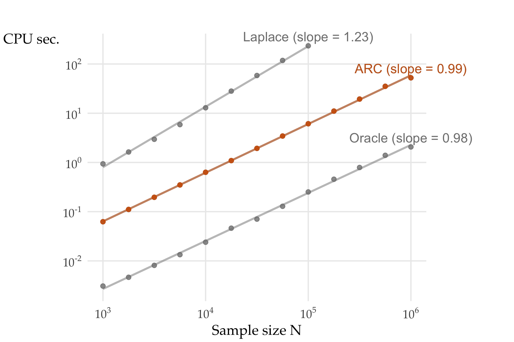
Figure 1: Time in seconds versus sample size $N$ for the Imb-Nul-Hi setting for all three algorithms: Laplace, ARC and the Oracle.

4.3 Regression coefficient estimation

Next, we turn to estimation of the regression coefficients, treating the intercept differently from the others. The intercept poses a challenge because it is somewhat confounded with the random effects. For instance, if we replace $\beta_{0}$ by $\beta_{0}+\lambda$ while replacing $a_{i}$ by $a_{i}-\lambda$ then $Y_{ij}$ are unchanged. Large $\lambda$ would change $\bar{a}=(1/R)\sum_{i=1}^{R}a_{i}$ by an implausible amount that should be statistically detectable given that $a_{i}\sim\mathcal{N}(0,\sigma^{2}_{A})$. On the other hand $|\lambda|=O(\sigma_{A}/\sqrt{R})$ would be hard to detect statistically. The other regression parameters are not similarly confounded with main effects in our settings. We note that when a predictor is a categorical variable that is either a function of the row index $i$ or of the column index $j$, then it can be subject to some confounding similar to the intercept’s confounding. This was observed in Ghosh et al., 2022b .

Because of the confounding described above, we anticipate that the true MSE rate for the intercept cannot be better than $\mathcal{O}(\min\{R,C\}))$ which is $\mathcal{O}(N^{-0.53})$ in our imbalanced settings and $\mathcal{O}(N^{-0.56})$ in our balanced settings. For the other coefficients $\mathcal{O}(N^{-1})$ is not ruled out by this argument.

Figures 2 and 3 reports the mean square errors for the intercept and the coefficient of the first predictor estimated for different sample sizes, for the three estimators under study in the Imb-Nul-Hi setting. We report here the plot only for the first predictor because the mean squared errors of the estimates of the seven regression coefficients were essentially equivalent. All three estimators show and MSE very close to $\mathcal{O}(N^{-1})$ for $\beta_{1}$. Where we anticipated an MSE no better than $\mathcal{O}(N^{-0.53})$ (imbalanced) or $\mathcal{O}(N^{-0.56})$ (balanced) for the intercept we saw slightly better MSEs with slopes between $-0.57$ and $-0.60$, confirming our expectation that the intercept would be harder to estimate than the regression coefficients.

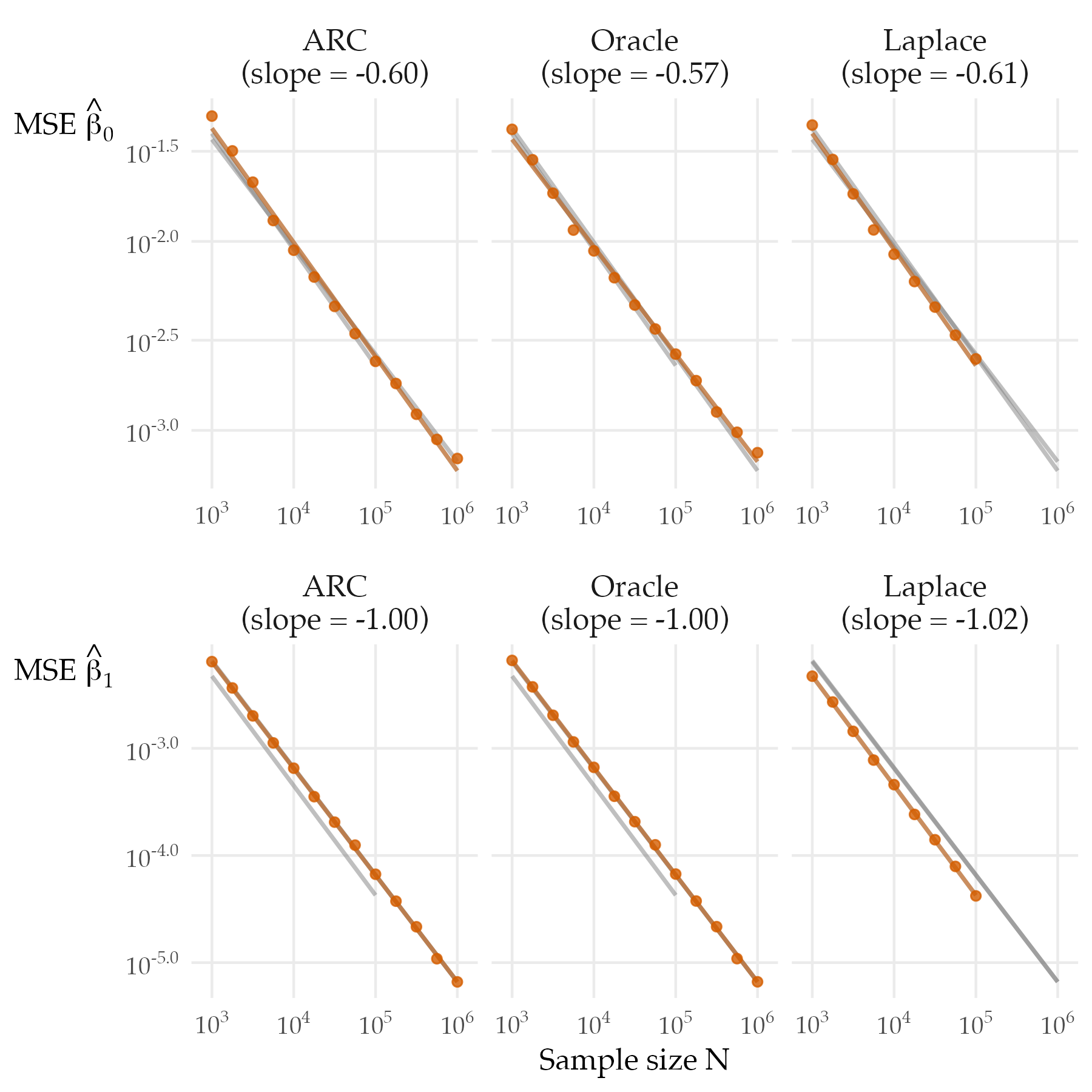
Figure 2: Mean squared errors for coefficient estimates in the Imb-Nul-Hi setting. The top row is for $\beta_{0}$ and the bottom row is for $\beta_{1}$. Each method is shown with a line and solid points and fitted reference lines for the other two methods (that overlap somewhat).

4.4 Variance component estimation

Here we present the estimation errors in the variance component parameters $\sigma_{A}$ and $\sigma_{B}$. The oracle method is given the true values of these parameters and so the comparison is only between ARC and the Laplace method.

For the variance parameter $\sigma^{2}_{A}$, the data only have $R$ levels $a_{1},\dots,a_{R}$. If they were observed directly, then we could estimate $\sigma^{2}_{A}$ by $(1/R)\sum_{i=1}^{R}a_{i}^{2}$ and have an MSE of $\mathcal{O}(R^{-1})$. In practice, the $a_{i}$ are obscured by the presence of the signal, the noise $\varepsilon_{ij}$ and the other random effects $b_{j}$. Accordingly, the best rate we could expect for $\sigma_{A}$ is $\mathcal{O}(R^{-1})=\mathcal{O}(N^{-\rho})$ and the best we could expect for $\sigma_{B}$ is $\mathcal{O}(C^{-1})=\mathcal{O}(N^{-\kappa})$.

Figure 3 shows the MSE for estimation of $\sigma_{A}$ and $\sigma_{B}$ for ARC and Laplace methods in the Imb-Nul-Hi setting. Due to the imbalance, our anticipated rates are $\mathcal{O}(N^{-0.88})$ for $\sigma_{A}$ and $\mathcal{O}(N^{-0.53})$ for $\sigma_{B}$. The ARC method does slightly better than these rates. The Laplace method attains nearly this predicted rate for $\sigma_{B}$ but does much worse for $\sigma_{A}$. We can understand both of these discrepancies in terms of biases, described next.

Figure 4 shows boxplots for the parameter estimates of $\sigma_{A}$ and $\sigma_{B}$ with the ARC and Laplce methods. We can compare the center of those boxplots to the reference line at the true parameter values and see that for the ARC estimates there is a bias decreasing at a faster rate than the width of the boxes. This explains the slightly better than predicted rates that we see for ARC. Instead the Laplace method has a substantial bias that only decreases very slowly as $N$ increases, giving Laplace a worse than expected rate, especially for $\sigma_{A}$.

We can understand the difficulties of the Laplace approximation method as follows. For $\sigma_{A}$ with $\rho=0.88$ the method has to approximate $\mathcal{O}(N^{0.88})$ integrals each of which typically has $\mathcal{O}(N^{1-0.88})=\mathcal{O}(N^{0.12})$ sample values. For $N=10^{3}$ this amounts to about $440$ integrals with an average of about $2.3$ observations each. For $N=10^{5}$ it is over 25,000 integrals with an average of just under $4$ observations each. This implies that the error in the Laplace approximation is asymptotically unbounded, and the resulting estimator might not even be consistent. More detailed results about this issue are reported in Ogden, (2021) for the case of random-intercept GLMMs; see also the Supplementary Material, § S1. The results of Ogden, (2021) are for hierarchical models. Crossed random effects are even more difficult as shown by Shun and McCullagh, (1995).

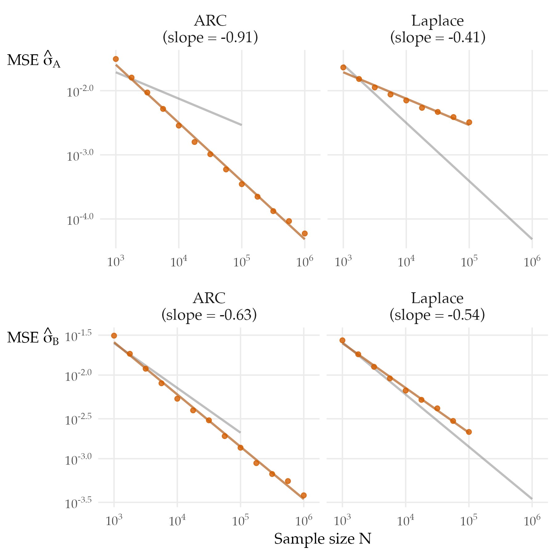
Figure 3: MSEs and estimated convergence rates for $\sigma_{A}$ and $\sigma_{B}$ for ARC and Laplace methods in setting Imb-Nul-Hi. In each plot there is a reference line for the covergence rate of the other method.

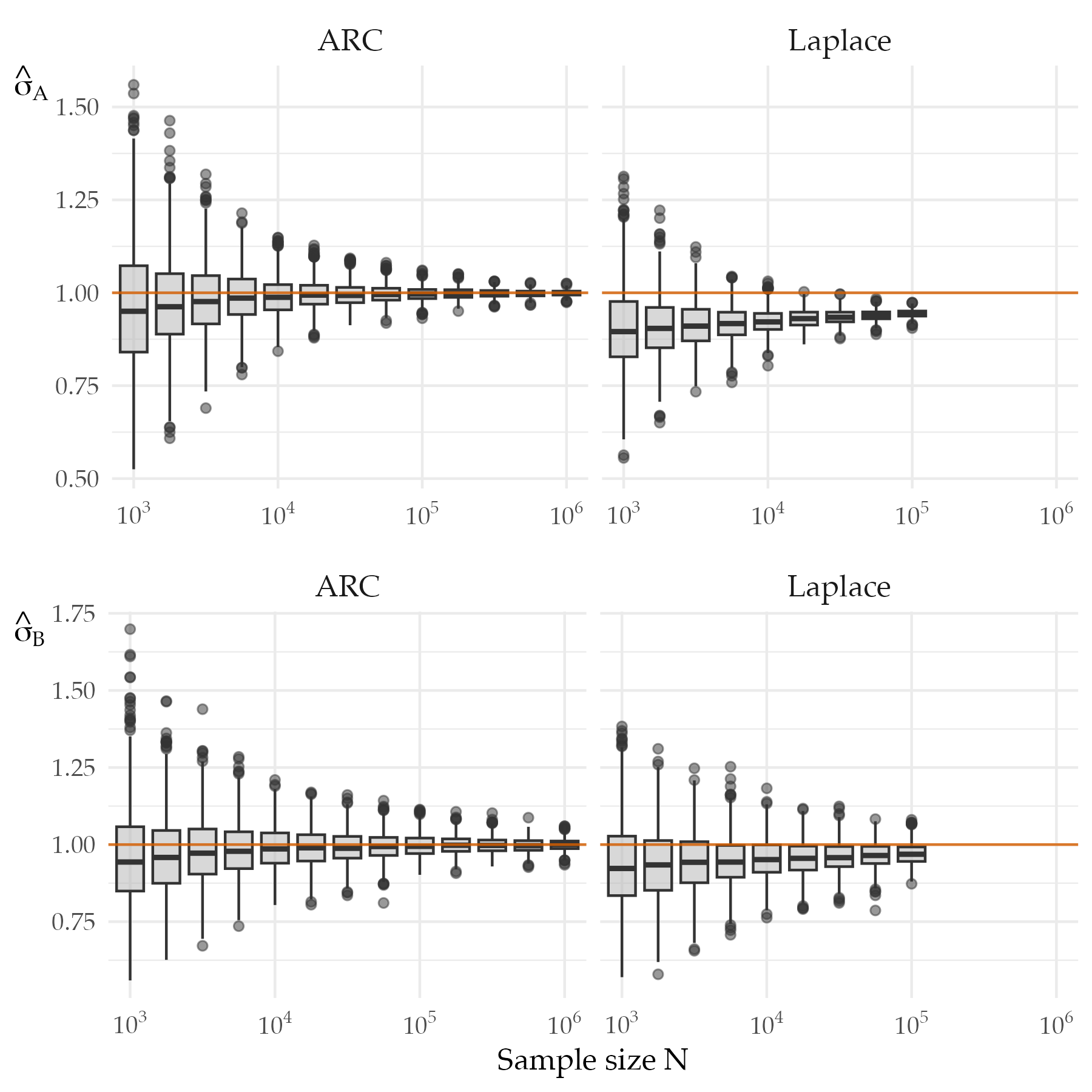
Figure 4: Boxplots of $\sigma_{A}$ and $\sigma_{B}$ estimates for the ARC and Laplace methods in the setting Imb-Nul-Hi. There are horizontal reference lines at the true parameter values. The ARC estimates have negative bias at small $N$ while the Laplace estimates have a strong extreme negative bias for all $N$.

4.5 Other settings

The simulation results for all eight settings, are reported in full in the Supplementary Figures S5–S44. We already discussed computational cost in eight settings based on Table LABEL:tab:timings. Here we make brief accuracy comparisons.

We compare our proposed ARC method to the oracle method which is infeasible because it requires knowledge of $\sigma_{A}$ and $\sigma_{B}$ and to the Laplace method which becomes infeasible for large $N$ because it does not scale as $\mathcal{O}(N)$. In most settings and for most parameters, the oracle method was slightly more accurate than ARC. That did not always hold. For instance in setting Bal-Lin-Hi (Figure S16) we see that ARC was slightly more accurate than the oracle method for $\beta_{1}$.

The figures in the Supplementary material show some cases where ARC has a slight advantage over the Laplace method and some where it has a slight disadvantage. There are a small number of cases where the Laplace method has outliers at $N=10^{3}$ that cause the linear regression slope to be questionable. These are present in setting Imb-Lin-Hi (Figure S22). However the attained MSEs at $N=10^{5}$ do not differ much between ARC and Laplace in that setting. Our conclusion is that compared to the Laplace method, ARC is scalable and robust.

4.6 Pairwise composite likelihood

The Supplementary Material Section S2 makes a comparison of ARC with the maximum pairwise likelihood estimator of Bellio and Varin, (2005). The comparison is made for the Imb-Nul-Hi setting that we have been focusing on.

From Section 2, the cost of pairwise composite likelihood is $\Omega(\max(N^{2}/R,N^{2}/C))=\Omega(\max(N^{2-\rho},N^{2-\kappa}))$. For the imbalanced setting this is $\Omega(N^{2-0.53})=\Omega(N^{1.47})$ We see in Section S2 that the empirical cost of the pairwise composite likelihood grows as $N^{1.42}$, close to the predicted rate. The empirical Laplace slope is $1.24$ there and the pairwise method has a cost curve that just barely crosses over the Laplace one at $N=10^{5}$.

The pairwise method attains very similar parameter estimation accuracy to ARC as judged by the reference lines and estimated slopes in Figures S2 and S3 of the Supplementary material. This holds for $\beta_{0}$, $\beta_{1}$, $\sigma_{A}$ and $\sigma_{B}$. Pairwise composite likelihood uses very accurate estimates of low dimensional integrals and it avoids the severe difficulty that the Laplace method has in this case. We do not see much evidence of ARC beating pairwise composite likelihood due to including information from triples and larger tuples of data within rows. However, this setting is dominated by small rows with correspondingly small numbers of triples. The most important difference for this example is that ARC costs $\mathrm{O}(N)$ while pairwise likelihood is far more expensive and does not scale to large data sets.

5 Application to the Stitch Fix Data

In this section we illustrate our ARC method on a data set from Stitch Fix. Quoting from Ghosh et al., 2022b :

Stitch Fix is an online personal styling service. One of their business models involves sending customers a sample of clothing items. The customer may keep and purchase any of those items and return the others. They have provided us with some of their client ratings data. That data was anonymized, void of personally identifying information, and as a sample it does not reflect their total numbers of clients or items at the time they provided it. It is also from 2015. While it does not describe their current business, it is a valuable data set for illustrative purposes.

In this data, the binary response $Y_{ij}$ of interest was whether customer $i$ thought that item $j$ was a top rated fit or not, with $Y_{ij}=1$ for an answer of ‘yes’. The predictor variables we used are listed in Table 2. Some of the categorical variable levels in the data had only a small number of levels. The table shows how we have aggregated them.

Variable	Description	Levels
Client fit	client fit profile	fitted
		loose or oversize
		straight or tight
Edgy	edgy style?	yes
		no
Boho	Bohemian style?	yes
		no
Chest	chest size	numeric
Size	dress size	numeric
Material	item primary material	artificial fiber
		leather or animal fiber
		regenerated fiber
		vegetable fiber
Item fit	item fit	fitted
		loose or oversized
		straight or tight

Table 2: Predictors available in the Stitch Fix data. There is one block of client predictors followed by a block of item predictors.

As anticipated in Section 2, we assume missing data at random and have removed rows with any missing entries. That leaves us with $N=4{,}965{,}960$ of the original $5{,}000{,}000$ ratings. We have data from $741{,}221$ clients on $3{,}523$ items. The data are not dominated by a single row or column because the customer with the most records accounts for only about $1.25\times 10^{-5}$ of them and the item with the most records accounts for at most $2.77\times 10^{-2}$ of them. The data are sparse because $N/(RC)\doteq 1.9\times 10^{-3}.$

In a business setting one would fit and compare a wide variety of different binary regression models in order to understand the data. Our purpose here is to study large scale probit models with including crossed random effects and so we choose just one model for illustration. We consider the probit model with crossed random effects whose fixed effects are specified according to the symbolic model formula:

Top $\sim$ Client fit + Edgy + Boho + Chest + Size + Material + Item fit,

where Top is the binary response variable described earlier. The model has $p=12$ parameters for fixed effects including the intercept. The first level of each categorical predictor in alphabetical order (Table 2) is used as the reference level in fitting the model.

Table 3 reports 1) the maximum likelihood estimates of the regression parameters under a marginal probit model that ignores the customer and item heterogeneity, and 2) the ARC estimates for the probit model with two crossed random effects for the customers and items. The z values reported in the table are computed with the observed information for the marginal probit model and with the two-way cluster-robust sandwich estimator described in Section 3.4. The ARC estimates of the variance components are $\hat{\sigma}_{A}=0.53$ and $\hat{\sigma}_{B}=0.34$. As expected, ignoring the customer and item heterogeneity lead to a large underestimation of the uncertainty in the parameter estimates and thus in the marginal probit all the predictors are strongly significant given the very large sample size. Conversely, the cross-random effects model takes into account the sources of heterogeneity and leads us to learn that the item fit is not a significant predictor of the top rank and that items made by vegetable fibers are less likely to be ranked top compared to clothes made by artificial fibers.

		Marginal probit			Probit with random effects
Variable		Est.${}^{\text{\textdagger}}$	z value	p value	Est.${}^{\text{\textdagger}}$	z value	p value
Intercept		$\phantom{-}43.1$	31.64	$<0.001$	$\phantom{-}50.9$	10.52	$<0.001$
Client fit	loose or oversize	$\phantom{-}8.7$	61.04	$<0.001$	10.3	10.81	$<0.001$
	straight or tight	$\phantom{-}5.1$	34.30	$<0.001$	6.0	10.67	$<0.001$
Edgy	yes	$-$3.0	$-$25.08	$<0.001$	$-$3.5	$-$7.49	$<0.001$
Boho	yes	$\phantom{-}8.9$	76.25	$<0.001$	10.5	25.81	$<0.001$
Chest		$-$0.5	$-$12.30	$<0.001$	$-$0.6	$-$7.32	$<0.001$
Size		$\phantom{-}0.2$	10.94	$<0.001$	0.3	2.99	$0.003$
Material	leather or animal	$-$12.9	$-$12.99	$<0.001$	$-$15.2	$-$1.57	0.116
	regenerated	$\phantom{-}2.5$	20.06	$<0.001$	$\phantom{-}3.0$	0.65	0.516
	vegetable	$-$12.2	$-$58.39	$<0.001$	$-$14.5	$-$3.13	$0.002$
Item fit	loose or oversized	9.7	36.15	$<0.001$	11.4	1.78	0.075
	straight or tight	$-2.1$	$-$9.55	$<0.001$	$-$2.5	$-$0.67	0.500

Table 3: Stitch Fix Binary Regression Results. ${}^{\text{\textdagger}}$All the estimated predictor parameters are multiplied by 100. Nonsignificant p values are marked in bold. See Table 2 for a description of the predictors. The first level of each categorial predictor in alphabetic order is used as reference level.

Variable		Naive	Sandwich	Pigeonhole
Intercept		1.36	4.84	5.08
Client fit	loose or oversize	0.14	0.95	0.96
	straight or tight	0.15	0.57	0.63
Edgy	yes	0.12	0.47	0.50
Boho	yes	0.12	0.41	0.49
Chest		0.04	0.08	0.11
Size		0.02	0.09	0.10
Material	leather or animal	0.99	9.65	9.24
	regenerated	0.21	4.62	4.24
	vegetable	0.13	4.59	4.23
Item fit	loose or oversized	0.27	6.42	6.32
	straight or tight	0.22	3.74	3.45

Table 4: Binary regression standard errors for the Stitch Fix data, computed three ways. Naive are the classical standard errors for the maximum likelihood estimates of the marginal probit model. Sandwich are the two-way clustered robust standard errors. Pigeonhole are non-parametric bootstrap standard errors described in Owen, (2007).All standard errors are multiplied by 100.

Table 5 compares the naive standard errors based on the classic probit output with two nonparametric methods that account for dependence. The nonparametric methods are in close agreement. The naive values correspond to variances underestimated by factors ranging from 4 to just over 1240, depending on the parameter and only slightly on whether we use sandwich or pigeonhole estimates of the coefficient variances. We also computed parametric bootstrap standard errors (not shown). Those were in between the naive ones and the nonparametric ones.

Figure 5 compares the two-way cluster robust sandwich standard errors with 1) the naive standard errors from a probit fit ignoring dependence between items and customers and 2) the pigeonhole nonparametric bootstrap standard errors of Owen, (2007) mentioned in Section 3.4. The figure shows how closely the sandwich and pigeonhole standard errors agree, while the naive standard errors are much smaller.

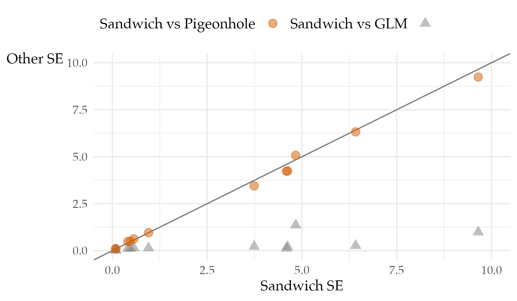
Figure 5: Stitch Fix Application. Comparison between the two-way cluster robust sandwich standard errors (x axis), the naive GLM standard errors (y axis, triangles) and the Pigeonhole nonparametric bootstrap standard errors (y axis, circles). The gray reference line is the first quadrant bisector $y=x$. All standard errors are multiplied by 100 as in Table 4.

6 Conclusions

We have developed a method for crossed random effects for binary regression. It is a probit version of composite likelihood that, by exploiting the connection between the Gaussian latent variables and the Gaussian random effects in this model, makes for very convenient factors in the composite likelihood. We find in simulations that the method costs $\mathcal{O}(N)$ and is competitive with and even more robust than a computationally infeasible Laplace approximation.

One surprise in this work was the difficulty of getting good approximations to even the one dimensional Gaussian integrals that arise. We are grateful for the insights in Ogden, (2021) and Shun and McCullagh, (1995). We surmise that the difficulties in multidimensional integration for random effects models on big data sets must be even more severe than the univariate ones we saw.

References

- Agresti, (2002) Agresti, A. (2002). Categorical Data Analysis. Wiley, New York.
- Albert and Anderson, (1984) Albert, A. and Anderson, J. A. (1984). On the existence of maximum likelihood estimates in logistic regression models. Biometrika, 71(1):1–10.
- Amemiya, (1985) Amemiya, T. (1985). Advanced Econometrics. Harvard university press.
- Andersen and Gill, (1982) Andersen, P. K. and Gill, R. D. (1982). Cox’s regression model for counting processes: a large sample study. The Annals of Statistics, 10(4):1100–1120.
- Bartolucci et al., (2017) Bartolucci, F., Chiaromonte, F., Don, P. K., and Lindsay, B. G. (2017). Composite likelihood inference in a discrete latent variable model for two-way “clustering-by-segmentation” problems. Journal of Computational and Graphical Statistics, 26(2):388–402.
- Bellio and Varin, (2005) Bellio, R. and Varin, C. (2005). A pairwise likelihood approach to generalized linear models with crossed random effects. Statistical Modelling, 5(3):217–227.
- Brooks et al., (2017) Brooks, M. E., Kristensen, K., van Benthem, K. J., Magnusson, A., Berg, C. W., Nielsen, A., Skaug, H. J., Maechler, M., and Bolker, B. M. (2017). glmmTMB balances speed and flexibility among packages for zero-inflated generalized linear mixed modeling. The R Journal, 9(2):378–400.
- Cameron et al., (2011) Cameron, C. A., Gelbach, J. B., and Miller, D. L. (2011). Robust inference with multiway clustering. Journal of Business & Economic Statistics, 29(2):238–249.
- Cox and Reid, (2004) Cox, D. and Reid, N. (2004). A note on pseudolikelihood constructed from marginal densities. Biometrika, 91(3):729–737.
- Eddelbuettel, (2013) Eddelbuettel, D. (2013). Seamless R and C++ Integration with Rcpp. Springer, New York. ISBN 978-1-4614-6867-7.
- Edelman and Rao, (2005) Edelman, A. and Rao, N. R. (2005). Random matrix theory. Acta Numerica, 14:233–297.
- Gao and Owen, (2017) Gao, K. and Owen, A. (2017). Efficient moment calculations for variance components in large unbalanced crossed random effects models. Electronic Journal of Statistics, 11(1):1235–1296.
- Gao and Owen, (2020) Gao, K. and Owen, A. B. (2020). Estimation and inference for very large linear mixed effects models. Statistica Sinica, 30(4):1741–1771.
- Ghandwani et al., (2023) Ghandwani, D., Ghosh, S., Hastie, T., and Owen, A. B. (2023). Scalable solution to crossed random effects model with random slopes. Technical report, arXiv:2307.12378.
- Ghosh, (2022) Ghosh, S. (2022). Scalable Inference for Crossed Random Effects Models. PhD thesis, Stanford University.
- (16) Ghosh, S., Hastie, T., and Owen, A. B. (2022a). Backfitting for large scale crossed random effects regressions. The Annals of Statistics, 50(1):560–583.
- (17) Ghosh, S., Hastie, T., and Owen, A. B. (2022b). Scalable logistic regression with crossed random effects. Electronic Journal of Statistics, 16(2):4604–4635.
- Ghosh and Zhong, (2021) Ghosh, S. and Zhong, C. (2021). Convergence rate of a collapsed Gibbs sampler for crossed random effects models. Technical report, arXiv:2109.02849.
- Heagerty and Lele, (1998) Heagerty, P. J. and Lele, S. R. (1998). A composite likelihood approach to binary spatial data. Journal of the American Statistical Association, 93(443):1099–1111.
- Jiang, (2010) Jiang, J. (2010). Large Sample Techniques for Statistics. Springer.
- Jiang, (2013) Jiang, J. (2013). The subset argument and consistency of MLE in GLMM: Answer to an open problem and beyond. The Annals of Statistics, 41(1):177–195.
- Jin and Andersson, (2020) Jin, S. and Andersson, B. (2020). A note on the accuracy of adaptive Gauss–Hermite quadrature. Biometrika, 107(3):737–744.
- Kristensen et al., (2016) Kristensen, K., Nielsen, A., Berg, C. W., Skaug, H., and Bell, B. M. (2016). TMB: Automatic differentiation and Laplace approximation. Journal of Statistical Software, 70(5):1–21.
- Kuk, (2007) Kuk, A. Y. C. (2007). A hybrid pairwise likelihood method. Biometrika, 94(4):939–752.
- Lindsay, (1988) Lindsay, B. G. (1988). Composite likelihood methods. Contemporary Mathematics, 80:221–239.
- Liu and Pierce, (1994) Liu, Q. and Pierce, D. A. (1994). A note on Gauss-Hermite quadrature. Biometrika, 81(3):624–629.
- Lumley and Mayer Hamblett, (2003) Lumley, T. and Mayer Hamblett, N. (2003). Asymptotics for marginal generalized linear models with sparse correlations. Technical report, University of Washington.
- McCullagh, (2000) McCullagh, P. (2000). Resampling and exchangeable arrays. Bernoulli, 6(2):285–301.
- Miglioretti and Heagerty, (2004) Miglioretti, D. L. and Heagerty, P. J. (2004). Marginal modeling of multilevel binary data with time-varying covariates. Biostatistics, 5(3):381–398.
- Miglioretti and Heagerty, (2007) Miglioretti, D. L. and Heagerty, P. J. (2007). Marginal modeling of nonnested multilevel data using standard software. American journal of epidemiology, 165(4):453–463.
- Ochi and Prentice, (1984) Ochi, Y. E. and Prentice, R. L. (1984). Likelihood inference in a correlated probit regression model. Biometrika, 71(3):531–543.
- Ogden, (2021) Ogden, H. (2021). On the error in Laplace approximations of high-dimensional integrals. Stat, 10(1):e380.
- Owen, (1990) Owen, A. B. (1990). Empirical likelihood ratio confidence regions. The annals of statistics, 18(1):90–120.
- Owen, (2007) Owen, A. B. (2007). The pigeonhole bootstrap. The Annals of Applied Statistics, 1(2):386–411.
- Papaspiliopoulos et al., (2020) Papaspiliopoulos, O., Roberts, G. O., and Zanella, G. (2020). Scalable inference for crossed random effects models. Biometrika, 107(1):25–40.
- R Core Team, (2023) R Core Team (2023). R: A Language and Environment for Statistical Computing. R Foundation for Statistical Computing, Vienna, Austria.
- Schall, (1991) Schall, R. (1991). Estimation in generalized linear models with random effects. Biometrika, 78(4):719–727.
- Shun and McCullagh, (1995) Shun, Z. and McCullagh, P. (1995). Laplace approximation of high dimensional integrals. Journal of the Royal Statistical Society Series B, 57(4):749–760.
- Silvapulle, (1981) Silvapulle, M. J. (1981). On the existence of maximum likelihood estimators for the binomial response models. Journal of the Royal Statistical Society. Series B (Methodological), pages 310–313.
- Skaug, (2002) Skaug, H. J. (2002). Automatic differentiation to facilitate maximum likelihood estimation in nonlinear random effects models. Journal of Computational and Graphical Statistics, 11(2):458–470.
- Stringer and Bilodeau, (2022) Stringer, A. and Bilodeau, B. (2022). Fitting generalized linear mixed models using adaptive quadrature. arXiv preprint arXiv:2202.07864.
- Varin et al., (2011) Varin, C., Reid, N., and Firth, D. (2011). An overview of composite likelihood methods. Statistica Sinica, 21(1):5–42.
- Xu et al., (2022) Xu, X., Reid, N., and Xu, L. (2022). Note on information bias and efficiency of composite likelihood. Statistica Sinica. Preprint No: SS-2022-0167.