A differential approach to investigate universal scaling in far-from-equilibrium quantum systems

Abstract

Recent progress in out-of-equilibrium closed quantum systems has significantly advanced the understanding of mechanisms behind their evolution towards thermalization. Notably, the concept of non-thermal fixed points (NTFPs) - responsible for the emergence of spatio-temporal universal scaling in far-from-equilibrium systems - has played a crucial role in both theoretical and experimental investigations. In this work, we introduce a differential equation that has the universal scaling associated with NTFPs as a solution. The advantage of working with a differential equation, rather than only with its solution, is that we can extract several insightful properties not necessarily present in the solution alone. Employing two limiting cases of the equation, we determined the universal exponents related to the scaling using the distributions near just two momentum values. We established a strong agreement with previous investigations by validating this approach with three distinct physical systems. This consistency highlights the universal nature of scaling due to NTFPs and emphasizes the predictive capabilities of the proposed differential equation. Moreover, under specific conditions, the equation predicts a power-law related to the ratio of the two universal exponents, leading to implications concerning particle and energy transport. This suggests that the observed power-laws in far-from-equilibrium turbulent fluids could be related to the universal scaling due to NTFPs, potentially offering new insights into the study of turbulence.

Introduction.— The field of out-of-equilibrium closed quantum systems encompasses many challenges, and recent times have witnessed remarkable progress in addressing many of these difficulties. A central pursuit in this field is untangling the mechanisms and routes responsible for taking non-equilibrium quantum systems towards thermalization. This topic is present in many areas of physics spanning all scales, from cosmological to particle physics systems Polkovnikov et al. (2011). Specifically, concepts such as pre-thermalization Baier et al. (2001); Micha and Tkachev (2003); Berges et al. (2004); Barnett et al. (2011); Nowak et al. (2014); Berges et al. (2014); Ueda (2020) and non-thermal fixed points (NTFPs) Scheppach et al. (2010); Berges et al. (2015) have contributed notably to advances in both theoretical understanding and experimental exploration of far-from-equilibrium systems.

Recently, a proposition has surfaced regarding classifying out-of-equilibrium quantum systems in universality classes Schmidt et al. (2012); Nowak et al. (2013). This concept parallels the notion of universality that emerges from fixed points observed in phase transition theories of systems in equilibrium. This dynamical analogue introduces the idea of NTFPs, which are metastable states within quantum many-body systems driven far from equilibrium. In proximity to these points, systems exhibit a notable independence of their initial conditions, with their dynamic evolution described by only a few parameters. These theoretical constructs are useful in interpreting various out-of-equilibrium phenomena more broadly Nowak et al. (2012); Karl et al. (2013); Piñeiro Orioli et al. (2015); Schmied et al. (2019); Chantesana et al. (2019).

Experiments involving cold atoms in the quantum regime have provided a unique platform for testing novel theories, such as the universal scaling in the neighborhood of NTFPs Madeira and Bagnato (2022). Particularly, compelling scenarios include quantum turbulence Madeira et al. (2020) achieved in Bose-Einstein condensates (BECs) García-Orozco et al. (2022) and quenches in cold atom gases Nicklas et al. (2015); Prüfer et al. (2018); Eigen et al. (2018); Erne et al. (2018); Glidden et al. (2021a); Gałka et al. (2022); Lannig et al. (2023). These systems provide time-evolving quantities which can be measured and compared against theoretical predictions.

This work presents compelling evidence that the phenomenon of universal scaling follows a well-defined differential equation, leading to the emergence of insightful properties. One can obtain accurate estimations for the exponents governing the universality class by examining two limiting cases. We demonstrate the validity of these principles through their application to three experimental investigations García-Orozco et al. (2022); Prüfer et al. (2018); Glidden et al. (2021a). Additionally, the equation predicts a power-law behavior near time-independent momentum distribution regions, and its characteristic exponent is related to the NTFP universal exponents.

NTFPs and universal scaling.— It has been suggested that out-of-equilibrium closed systems, falling within a specific universality category, manifest their self-similar behavior via their time-evolving momentum distribution $n(k,t)$ Schmidt et al. (2012); Nowak et al. (2013). When in the vicinity of a NTFP, this distribution obeys temporal and momentum scaling, adhering to the form:

$$n(k,t)=\left(\frac{t}{t_{0}}\right)^{\alpha}F\left[\left(\frac{t}{t_{0}}\right)^{\beta}k\right],$$ (1)

where $t_{0}$ is an arbitrary reference (restricted to the temporal window where universal scaling is observed) and $F(k)$ is the corresponding universal function. This distinctive behavior emerges due to metastable regions within specific time intervals and momentum ranges and depends on two universal exponents. The $\alpha$ and $\beta$ exponents are related to amplitude adjustments and scale renormalizations, respectively. The traditional approach to investigating NTFPs involves perturbing the system from its equilibrium state and tracking the evolution of the momentum distribution $n(k,t)$.

Differential equation.— Verifying if numerical or experimental data displays the universal scaling of Eq. (1), that is, if for a specific time interval and momentum range, two exponents make all the momentum distributions collapse into a single universal function $F(k)$, has been the standard approach to identifying the presence of NTFPs. Delineating a different approach, we found additional properties nested within the non-equilibrium quantum system as it navigates its route towards thermalization.

We begin our exploration by focusing on an out-of-equilibrium system defined by the distribution $n(k,t)$ at a specific moment in time. As we track the progression of the system from time $t$ to $t+dt$, each variable may change, allowing us to express the collective variation in the distribution as follows:

$$dn(k,t)=\frac{\partial n}{\partial t}\Bigg{|}_{k}dt+\frac{\partial n}{\partial k}\Bigg{|}_{t}dk.$$ (2)

To observe scaling, we must allow both amplitude and momentum scale variations to be time-parameterized. We assume a particular form for these time dependences,

$$\frac{dn}{n}\Bigg{|}_{k} = \alpha\frac{dt}{t},$$ (3)

$$\frac{dk}{k} = \beta\frac{dt}{t}.$$ (4)

Here, $\alpha$ and $\beta$ denote the exponents governing the temporal amplitude and momentum scale changes, respectively. Modest magnitudes of $\alpha$ and $\beta$ imply a slow evolution of the system, whereas the limiting case of $\alpha=\beta=0$ corresponds to a stationary state, indicating equilibrium.

Guided by these insights, the complete variation of $n(k,t)$ can be expressed in differential form as:

$$t\frac{\partial n(k,t)}{\partial t}=\alpha n(k,t)+\beta k\frac{\partial n(k,t)}{\partial k}.$$ (5)

This equation contains the interplay between temporal changes in amplitude and momentum scale considering the power-law behaviors, Eqs. (3) and (4), exhibited by both attributes. If $\alpha$ and $\beta$ remain constant, a solution of this equation is Eq. (1). The advantage of working with a differential equation, rather than only with its solution, is that we can extract several insightful properties not necessarily present in Eq. (1).

At this point, we can examine two limiting scenarios. The first case concerns momentum ranges where the amplitude of the momentum distribution undergoes negligible temporal variation, essentially characterizing regions of minimal change over time, we can neglect the $\partial n/\partial t$ term. Consequently, we arrive at:

$$\frac{\partial n}{\partial k}\Bigg{|}_{t}=-\frac{\alpha}{\beta}\frac{n}{k},$$ (6)

yielding a solution applicable to this scenario of temporal stagnation,

$$n(k,t)\propto k^{-\alpha/\beta}\text{ (if $n$ is time-independent)},$$ (7)

thus exhibiting a power-law behavior within this specific region.

Similarly, another interesting limit is $k\to 0$, deep in the infrared (IR) region. In this limit, Eq. (5) anticipates

$$n(k\to 0,t)\propto t^{\alpha},$$ (8)

consistent with taking the same limit directly in Eq. (1). Equations (7) and (8) show that when an out-of-equilibrium system approaches an NTFP, it is possible to determine the exponents $\alpha$ and $\beta$ governing its evolution without the need to scale all curves to validate their collapse onto a universal curve.

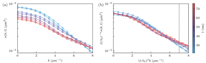
Figure 1: Distributions and their collapse onto universal curves described by Eq. (1). (a) Momentum distribution of a turbulent state of a harmonically trapped three-dimensional Bose gas for an excitation amplitude of $A=2\mu_{0}$ and (b) its scaling with $\alpha=-0.50(8)$ and $\beta=-0.2(4)$ García-Orozco et al. (2022). The dashed line indicates the IR region where the universal dynamics is observed. (c) Momentum distribution for a quenched three-dimensional Bose gas, and (d) its corresponding IR scaling with $\alpha=1.15(8)$ and $\beta=0.34(5)$ Glidden et al. (2021a, b). (e) Structure factor of a spinor Bose gas driven far from equilibrium and (f) the universal scaling with $\alpha=0.33(8)$ and $\beta=0.54(6)$ Prüfer et al. (2018).

NTFPs in experiments with cold atoms.— Many experimental investigations have employed cold atom gases as platforms to observe systems near NTFPs García-Orozco et al. (2022); Nicklas et al. (2015); Prüfer et al. (2018); Eigen et al. (2018); Erne et al. (2018); Glidden et al. (2021a); Gałka et al. (2022); Lannig et al. (2023). Here, we focus on three of them, which used very different physical systems and mechanisms to drive the system to far-from-equilibrium states. In Ref. García-Orozco et al. (2022), the authors investigated the emergence of universal scaling due to NTFPs in a harmonically trapped three-dimensional (3D) Bose gas driven to a turbulent state. A sinusoidal time-varying magnetic field gradient produced a far-from-equilibrium state. The amplitude $A$ of the excitation could be varied, and for three of its values, the authors showed that dynamical scaling emerges. Figure 1a shows the time evolution of the momentum distribution of a turbulent state. As time passes, the distribution shifts towards high momenta, indicating the depletion of the condensate. The scaling employing Eq. (1) with $\alpha=-0.50(8)$ and $\beta=-0.2(4)$ is shown in Figure 1b, which collapses all curves into a single function. These results are for an excitation amplitude of $A=2\mu_{0}$, where $\mu_{0}$ is the chemical potential at the center of the cloud. For the other amplitudes, the reader is referred to Sup .

Next, we consider Ref. Glidden et al. (2021a), where the authors observed bidirectional dynamical scaling in a three-dimensional Bose gas Gaunt et al. (2013). This phenomenon was observed in the IR and the ultraviolet (UV) regions of the momentum distribution, although here we will focus on the IR scaling. Despite distinct exponents for universal scaling in each region, these values do not correspond to separate NTFPs. Instead, they arise due to particle and energy transport following NTFP theory Schmied et al. (2019). The experimental strategy involved rapidly removing atoms and energy by turning off interatomic interactions and lowering the trap depth, inducing a far-from-equilibrium state. Turning on the interactions initiated thermalization. Figure 1c, produced with the data available in Ref. Glidden et al. (2021b), illustrates unscaled $n(k,t)$ profiles, while the IR region displays universal behavior with $\alpha=1.15(8)$ and $\beta=0.34(5)$, as seen in Fig. 1d.

The third system we consider was investigated in Ref. Prüfer et al. (2018), where authors observed universal dynamics using a quasi-one-dimensional spinor Bose gas Sadler et al. (2006). This was achieved through an analysis of spin correlations in a spin-1 system. With the initial state corresponding to all atoms occupying a single magnetic state, the departure from equilibrium was induced by an abrupt alteration in the energy splitting of sublevels, thus producing excitations. In this case, the relevant quantity to observe the universal scaling of Eq. (1) is a structure factor, which depends on momentum and time just as the momentum distribution. In Fig. 1e, we reproduce the temporal evolution of the structure factor $f_{\theta}(k,t)$ using the data provided by the authors Prüfer et al. (2018). There is a discernible shift towards lower momenta as time passes. Applying the scaling of Eq. (1) with $\alpha=0.33(8)$ and $\beta=0.54(6)$ to the data results in the convergence of all points onto a universal curve, as depicted in Fig. 1f.

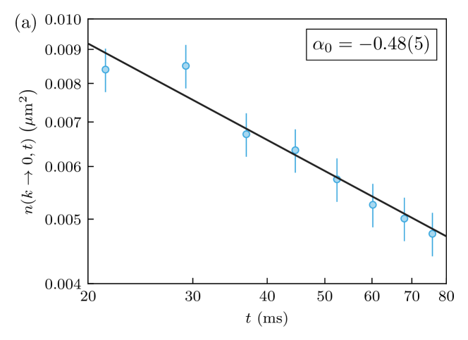
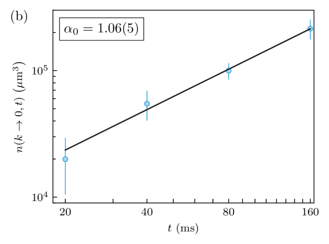
Figure 2: Low-momentum ($k\to 0$) behavior of the distributions as a function of time for (a) a turbulent BEC García-Orozco et al. (2022), (b) quenched Bose gas Glidden et al. (2021a), and (c) spinor Bose gas Prüfer et al. (2018). The solid curves correspond to a fit to the functional form provided by Eq. (8), which yield $\alpha$ values in excellent agreement with the ones reported by the authors. The uncertainties were not available for Ref. Prüfer et al. (2018).

Results.— References García-Orozco et al. (2022); Glidden et al. (2021a); Prüfer et al. (2018) employed statistical analyses to determine the universal exponents $\alpha$ and $\beta$ that collapse the distributions for a momentum range and time interval onto a single function. These procedures employ all the experimental points in the considered interval. However, if the scaling interval contains the $k\approx 0$ region, Eq. (8) is a much simpler way of determining $\alpha$. In Fig. 2, we show the time evolution of each distribution for the smallest momentum measured. A fit to the functional form of Eq. (8) provides an estimate of the value of $\alpha$, in excellent agreement with the ones found in Refs. García-Orozco et al. (2022); Glidden et al. (2021a); Prüfer et al. (2018). We summarize the results in Tab. 1.

Having determined $\alpha$ from the $k\to 0$ behavior of the distributions, we now focus on obtaining the value of $\beta$. Figure 1 shows that the unscaled curves for the three physical systems all possess a momentum value where the distribution is approximately time-independent, which we denote by $k^{*}$. In the vicinity of this point, Eq. (5) can be used to determine the value of $\beta$,

$$\beta=-\frac{\alpha}{k^{*}}\frac{n(k^{*},t)}{(\partial n/\partial k)|_{k=k^{*}}}.$$ (9)

We employed Eq. (9) to compute the values of $\beta$ for the three physical systems of interest. The derivative has to be taken numerically, which can lead to large fluctuations when applied to experimental data. Using a central difference derivative, we found that the data of Ref. Prüfer et al. (2018) had to be smoothed to reduce the noise, and a three-point moving average was sufficient to prevent the fluctuations. Note that Eq. (9) yields a value of $\beta$ for each instant $t$; therefore, we report the average of the values and their uncertainty. Since Eq. (9) requires a value for $\alpha$, we considered two cases: the value found with the $k\to 0$ behavior of the distributions and the one reported by the authors of Refs. García-Orozco et al. (2022); Glidden et al. (2021a); Prüfer et al. (2018). The results are summarized in Tab. 1.

Table 1: Universal exponents $\alpha$ and $\beta$. The columns “standard procedure” correspond to the values reported by the authors of Refs. García-Orozco et al. (2022); Glidden et al. (2021a); Prüfer et al. (2018). In the case of Ref. García-Orozco et al. (2022), three different excitation amplitudes were employed. The $\alpha_{0}$ values correspond to the $k\to 0$ approximation, see Fig. (2). Equation (9) was used to compute the values $\beta_{0}$ and $\beta_{1}$, the difference being which value of $\alpha$ was employed. All approximations are in excellent agreement with the values reported in Refs. García-Orozco et al. (2022); Glidden et al. (2021a); Prüfer et al. (2018).

		Standard procedure	Taking the $k\to 0$ limit	Standard procedure	Near $k^{*}$ with $\alpha_{0}$	Near $k^{*}$ with $\alpha$
System		$\alpha$	$\alpha_{0}$	$\beta$	$\beta_{0}$	$\beta_{1}$
	A ($\mu_{0}$)
	1.8	-0.46(2)	-0.44(5)	-0.2(9)	-0.26(7)	-0.30(7)
Ref. García-Orozco et al. (2022)	2.0	-0.51(1)	-0.48(5)	-0.2(7)	-0.25(5)	-0.26(5)
	2.2	-0.50(2)	-0.49(5)	-0.2(9)	-0.37(8)	-0.38(9)
Ref. Glidden et al. (2021a)		1.15(8)	1.06(5)	0.34(5)	0.41(7)	0.45(7)
Ref. Prüfer et al. (2018)		0.33(8)	0.41(8)	0.54(6)	0.57(9)	0.46(7)

Finally, Eq. (7) predicts a power-law for $n(k,t)$ in a momentum range where the distribution is approximately time-independent. Inspection of each of the unscaled distributions in Fig. 1 reveals that, although we can identify a point $k^{*}$ where $(\partial n/\partial k)|_{k=k^{*}}\approx 0$, this condition is not rigorously observed in a finite $k$-range for neither of the three physical systems considered here. However, the beginning of the time evolution ($t\lesssim 6.5\;$s) of the spinor Bose gas fulfils this condition in good approximation for the range of $0.003\;\mu$m${}^{-1}\leqslant k\leqslant 0.009\;\mu$m^-1. Figure 3 shows the exponent obtained when we fitted the data in this region to a power-law functional form, $f_{\theta}(k,t)\propto k^{-\delta}$. We also included in the figure the theoretical prediction of Eq. (7), $\delta=\alpha/\beta=0.61(16)$, calculated with the values and uncertainties reported in Ref. Prüfer et al. (2018). The agreement is good for the early evolution ($t\lesssim 6.5\;$s), but for later times, the values of the structure factor change considerably, such that the premise of the theoretical prediction is inapplicable beyond this temporal threshold.

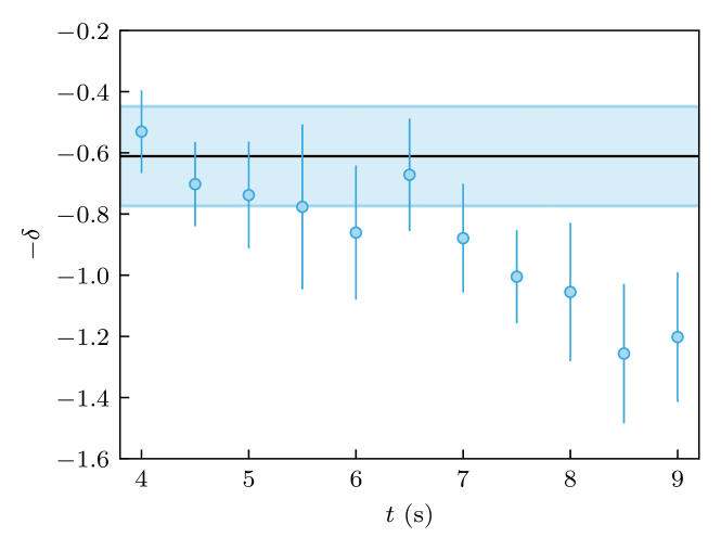
Figure 3: Exponent of a power-law $f_{\theta}(k,t)\propto k^{-\delta}$ fit near $k^{*}\approx 0.006\;\mu$m^-1 for the case of a spinor Bose gas Prüfer et al. (2018). The theoretical prediction of Eq. (7) is $\delta=\alpha/\beta=0.61(16)$, which is denoted by the black line and its uncertainty by the shaded blue area.

Conclusions.— In this work, we proposed a differential equation, Eq. (5), which has as a solution the well-known scaling due to the presence of NTFPs, Eq. (1). This allowed us to investigate features not evident or present in the solution alone. We then applied these properties to three distinct physical systems García-Orozco et al. (2022); Glidden et al. (2021a); Prüfer et al. (2018) and found that our predictions are in excellent agreement with previous investigations. The fact that the systems and the protocols for driving them out of equilibrium are so different stresses the universal character of the scaling due to NTFPs and the results from our differential equation.

First, from the $k\to 0$ behavior of the distributions, we obtained an estimate for the universal exponent $\alpha$. Although this considers only one data point for each time instant, which is undesirable when working with experimental data, the agreement with the values reported in Refs. García-Orozco et al. (2022); Glidden et al. (2021a); Prüfer et al. (2018) is remarkable.

Then, we identified a point, denoted by $k^{*}$, at which the temporal variation of the distributions is approximately null. This feature is present in the physical systems under investigation in this work and several other systems where universal scaling was observed Nicklas et al. (2015); Eigen et al. (2018); Erne et al. (2018); Gałka et al. (2022); Lannig et al. (2023). Using the differential equation and the variation of the distributions with respect to momentum, we estimated the values of $\beta$. Hence, with information about the distributions at the vicinity of just two momentum values, $k\to 0$ and $k^{*}$, we were able to compute the universal exponents $\alpha$ and $\beta$ in agreement with the values obtained through much more sophisticated procedures García-Orozco et al. (2022); Glidden et al. (2021a); Prüfer et al. (2018).

Equation (7) contains an interesting prediction: if the distribution is time-independent in a specific momentum range, then a power-law $\propto k^{-\alpha/\beta}$ is expected. Although the assumption of a constant distribution in a range is not strictly observed in the physical systems we considered, the early evolution of the spinor Bose gas agrees with the theoretical prediction reasonably.

Finally, another intriguing feature of Eq. (7) is that its power-law is related to the ratio of the two universal exponents, which has physical meaning under specific conditions. For that, let us define two quantities inside the region where scaling is observed, the mean particle number $\overline{N}$ and kinetic energy $\overline{E}$, which help us describe particle and energy transport. Using Eq. (1), we can write the temporal dependence of these quantities in terms of the dimension $d$ of the system and universal exponents,

$$\overline{N}(t) = \int d^{d}k\ n(k,t)\propto\left(\frac{t}{t_{0}}\right)^{\alpha-d\beta},$$ (10)

$$\overline{E}(t) \propto \int d^{d}k\ k^{2}n(k,t)\propto\left(\frac{t}{t_{0}}\right)^{\alpha-(d+2)\beta},$$ (11)

where we assumed a quadratic dispersion relation to compute $\overline{E}$. The integrals are over the scaled range ${\left(t/t_{0}\right)^{-\beta}k_{\ell}\leqslant|k|\leqslant\left(t/t_{0}\right)^{-\beta}k_{h}}$, and $k_{\ell}\leqslant k\leqslant k_{h}$ is the momentum range where the universal scaling is observed.

According to Eq. (10), particle-conserving transport requires $\alpha=d\beta$, while Eq. (11) dictates that energy-conserving transport is given by $\alpha=(d+2)\beta$ Chantesana et al. (2019); Schmied et al. (2019). Consequently, for these two types of conserving transports, $\alpha$ and $\beta$ assume the same sign, which is determined by the direction of the transport: positive towards the IR region and negative towards the UV region. Distinct momentum regions may exhibit different values for $\alpha$ and $\beta$, accompanied by different signs Glidden et al. (2021a).

Hence, Eq.(7) predicts a power-law $\propto k^{-d}$ for particle-conserving transport, while energy-conserving transport corresponds to $\propto k^{-(d+2)}$. These two situations are very relevant to the field of quantum turbulence Madeira et al. (2020). A standard approach to identify a turbulent state in a quantum fluid is the emergence of a power-law in the momentum distribution Thompson et al. (2013); Navon et al. (2016), indicating a particle cascade, or in the energy spectrum, a signal of an energy cascade. Our result suggests that the power-laws observed in turbulent fluids, which are far from equilibrium, could be intimately related to the universal scaling due to NTFPs. These results bring a new perspective to investigate the complex phenomenon of turbulence and merit further investigation.

Supplemental Material: A differential approach to investigate universal scaling in far-from-equilibrium quantum systems

In the main text, we provided the results for one of the excitation amplitudes of Ref. García-Orozco et al. (2022). Here, we also provide similar figures for the other two amplitudes. Figure S1 contains the distributions and their scaling, while Fig. S2 is related to the $k\to 0$ behavior of the distributions.

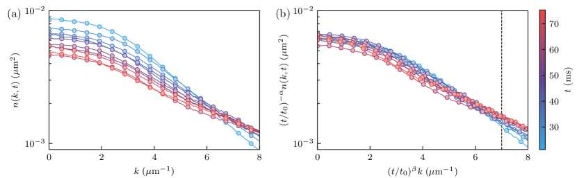
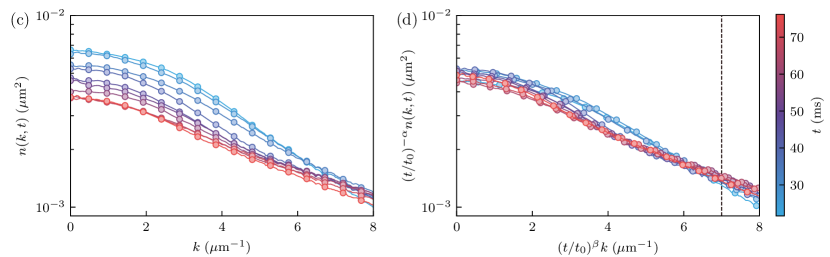
Figure S1: Momentum distributions of harmonically trapped three-dimensional Bose gases excited towards turbulence and their collapse onto universal curves described by Eq. (1). Momentum distribution for an excitation amplitude of (a) $A=1.8\mu_{0}$ and (c) $A=2.2\mu_{0}$. Universal scaling with $\alpha=-0.50(8)$ and $\beta=-0.2(4)$ García-Orozco et al. (2022) for (c) $A=1.8\mu_{0}$ and (d) $A=2.2\mu_{0}$.

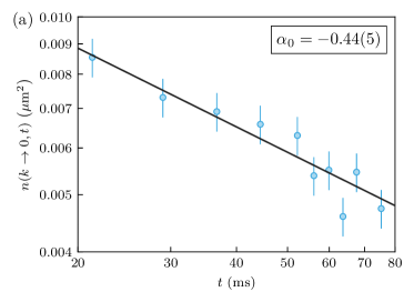
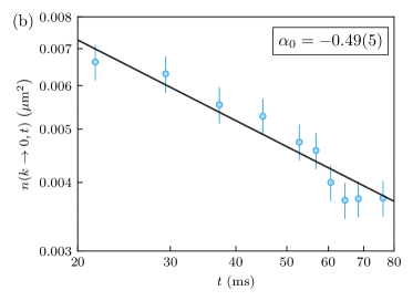
Figure S2: Low-momentum ($k\to 0$) behavior of $n(k,t)$ for turbulent states of harmonically trapped three-dimensional Bose gases as a function of time for excitation amplitudes of (a) $A=1.8\mu_{0}$ and (b) $A=2.2\mu_{0}$. The solid curves correspond to a fit to the functional form provided by Eq. (8).