Clustering Without an Eigengap

Abstract

We study graph clustering in the Stochastic Block Model (SBM) in the presence of both large clusters and small, unrecoverable clusters. Previous approaches achieving exact recovery do not allow any small clusters of size $o(\sqrt{n})$, or require a size gap between the smallest recovered cluster and the largest non-recovered cluster. We provide an algorithm based on semidefinite programming (SDP) which removes these requirements and provably recovers large clusters regardless of the remaining cluster sizes. Mid-sized clusters pose unique challenges to the analysis, since their proximity to the recovery threshold makes them highly sensitive to small noise perturbations and precludes a closed-form candidate solution. We develop novel techniques, including a leave-one-out-style argument which controls the correlation between SDP solutions and noise vectors even when the removal of one row of noise can drastically change the SDP solution. We also develop improved eigenvalue perturbation bounds of potential independent interest. Using our gap-free clustering procedure, we obtain efficient algorithms for the problem of clustering with a faulty oracle with superior query complexities, notably achieving $o(n^{2})$ sample complexity even in the presence of a large number of small clusters. Our gap-free clustering procedure also leads to improved algorithms for recursive clustering. Our results extend to certain heterogeneous probability settings that are challenging for alternative algorithms.

1 Introduction

Graph clustering is a fundamental problem with various applications to the study of diverse real-world networks, such as social, biological, and information networks. A standard approach for benchmarking clustering algorithms is to consider probabilistic models for generating a graph with a planted set of unknown, ground-truth clusters. Beyond their modeling power of practical networks, the study of such models over the past decades has led to notable theoretical advancement in the interface of combinatorial optimization, statistical learning, information theory and applied probability, greatly enriching our understanding of computational and statistical tradeoffs. For a survey of the algorithmic and theoretical work in this area, see Abbe (2018).

In this paper, we consider the canonical model called Stochastic Block Model (SBM), also known as the Planted Partition Model (Holland et al., 1983; Condon and Karp, 2001). We focus on the unbalanced clusters setting, formally defined below, where the planted clusters have different sizes.

As we discuss in greater details below, most existing results, with a few notable exceptions, require all clusters to be sufficiently large or the existence a gap between the large and small clusters. The goal of this paper is to eliminate such assumptions.

1.1 Problem Setup

Let $[n]:=\{1,\dots,n\}$ be a set of $n$ vertices partitioned into $K$ unknown clusters $V_{1},\dots,V_{K}$. We observe a random graph on these vertices with adjacency matrix $A\in\{0,1\}^{n\times n}$, where for two numbers $1\geq p>q\geq 0$, and independently across all $i\leq j$,

$$A_{ij}\sim\begin{cases}\text{Bernoulli}(p),&\text{if $i,j$ belong to the same cluster},\\ \text{Bernoulli}(q),&\text{if $i,j$ do not belong to the same cluster}.\end{cases}$$

and $A_{ij}=A_{ji}$ for all $i>j$. In other words, $p$ is the edge probability between two nodes in the same cluster, and $q$ is the probability between two nodes in different clusters. Note that $p,q$ and $K$ are allow to depend on $n$.

We let $(s_{1},\dots,s_{K})=(|V_{1}|,\dots,|V_{K}|)$ be the cluster sizes, where the sizes are ordered as $s_{1}\geq s_{2}\geq\dots s_{K}$. Since all our algorithms and analysis do not rely on the ordering of the vertices, we further assume, without loss of generality and for notational convenience, that the vertices are ordered by their cluster membership, so that $V_{1}=\{1,\dots,s_{1}\}$, $V_{2}=\{s_{1}+1,\dots,s_{1}+s_{2}\}$, and so on. We encode the ground truth clustering using a matrix $Y^{*}\in\{0,1\}^{n\times n}$, defined by setting $Y^{*}_{ij}=1$ if and only if $i$ and $j$ belong to the same cluster. By our ordering assumption $Y^{*}$ is block-diagonal and has the form $Y^{*}=\operatorname{diag}\left(J_{s_{1}\times s_{1}},\dots,J_{s_{K}\times s_{K}}\right)$, where $J_{m\times r}$ denotes an all-ones matrix of size $m\times r$. Note that the cluster sizes $\{s_{i}\}$ correspond to the eigenvalues of the $Y^{*}$. We assume that $p\geq\log n/n$, a common assumption in the literature and known to be necessary for exact recovery.

1.2 Algorithms and Prior Results for Unbalanced SBM

A plethora of algorithms have been developed for graph clustering, and many of them enjoy rigorous performance guarantees; see, for instance, McSherry (2001); Bollobás and Scott (2004); Chen et al. (2012); Chaudhuri et al. (2012); Vu (2018); Abbe (2018), and the references therein. Nearly all theoretical guarantees for the problem of exact recovery in the SBM require all clusters to be “large”, typically of size $\widetilde{\Omega}(\sqrt{n})$. Under such an assumption, these algorithms recover all clusters. From theoretical and practical standpoints, it is desirable to have algorithms which, despite the presence of “small” clusters below this threshold, provably recover all sufficiently large clusters. While this is a natural goal, establishing such a result is surprisingly nontrivial. Only two existing results allow the presence of small clusters, Ailon et al. (2013, 2015) and Mukherjee et al. (2022). Postponing the discussion of Mukherjee et al. (2022) to after presenting our main theorem (in Section 2), we discuss Ailon et al. (2013, 2015) below. In the sequel, we write $a_{n}\lesssim b_{n}$ or $a_{n}=O(b_{n})$ if $a_{n}\leq Cb_{n},\forall n$ for a universal numerical constant $C>0$.

Ailon et al consider a convex relaxation approach based on semidefinite programming (SDP). Their results allow for small clusters, but additionally assume there exists a constant multiplicative gap between the sizes of large and small clusters. Specifically, letting $\overline{s}>\underline{s}$ be two consecutive cluster sizes (i.e., there are no clusters with sizes in $(\underline{s},\overline{s})$), they guarantee exact recovery of all clusters with sizes at least $\overline{s}$ as long as the following conditions are satisfied:

$$\frac{(p-q)^{2}\overline{s}^{2}}{pn}\gtrsim\log n\qquad\text{and}\qquad\overline{s}/\underline{s}\gtrsim 1.$$ (1)

Under the above condition and after reordering nodes by cluster identity, their optimization program returns a block-diagonal solution of the form

$$\widehat{Y}=\operatorname{diag}\left(J_{s_{1}\times s_{1}},\dots,J_{\overline{s}\times\overline{s}},0_{\underline{s}\times\underline{s}},\dots,0_{s_{K}\times s_{K}}\right).$$ (2)

That is, all big clusters are exactly recovered and all small clusters are completely ignored.

The above result can be slightly improved and generalized. We present this improvement below and later prove using an argument significantly simpler than those in Ailon et al. (2013, 2015). This result illustrates the boundary of what can be proved using existing techniques, and serves as a warmup for our main result. These results are based on solving the following trace-regularized SDP:

$$\widehat{Y}=\operatorname*{argmax}_{Y\in\mathbb{R}^{n\times n}}\quad \left\langle Y,A-\frac{p+q}{2}J_{n\times n}\right\rangle-\lambda\operatorname{Tr}(Y)$$ (3a)

s.t. $$Y\succcurlyeq 0,$$ (3b)

$$0\leq Y_{ij}\leq 1,\forall i\in[n],j\in[n]$$ (3c)

where $\lambda$ is a regularization parameter which will be specified later. We refer to (3) as the recovery SDP. We note that this SDP and its variants, usually without the trace regularizer, are considered in many prior works; we refer to the survey Li et al. (2021) and the references therein, as well as Ames (2014), Chen and Xu (2014), Cai and Li (2015), and Amini and Levina (2018). For the SDP (3), we have the following slightly-improved, but still gap-dependent guarantee:

Theorem 1 (Informal version of Theorem 4).

If there exists two consecutive cluster sizes $\overline{s}>\underline{s}$ satisfying

$$\left(1-\underline{s}/\overline{s}\right)^{2}\frac{(p-q)^{2}\overline{s}^{2}}{pn}\gtrsim\log n$$ (4)

then with high probability the solution to the recovery SDP (3) with a suitable $\lambda$ is of the form (2).

This theorem improves upon the result in (1) because instead of requiring the size ratio $\overline{s}/\underline{s}$ between large and small clusters to be a large constant, it allows for the ratio to approach $1$ so long as the signal-to-noise ratio, $\frac{(p-q)^{2}\overline{s}^{2}}{pn}$ is proportionally larger.

Theorem 1 is, essentially, the furthest possible extension of Ailon et al. (2013, 2015), which aims for exact recovery in the sense of an SDP solution with diagonal blocks of either ones or zeroes.

We believe the essential limitation of both Theorem 1 and Ailon et al. (2013, 2015) that necessitates a gap assumption is not fundamentally algorithmic, but rather the form of their guarantees. Without assuming a gap in cluster sizes, there may exist clusters which are on the boundary of recoverability. In different typical samples from the same SBM instance, the recovery SDP (3) solution may or may not recover such clusters. Furthermore, the corresponding block of the SDP solution may not be all-one nor all-zero. Therefore, in the absence of a gap, it should not be possible to guarantee an SDP solution of the form 2, which consists of exclusively all-one or all-zero diagonal blocks. This is demonstrated experimentally in Figure 1(b), where the largest cluster is recovered with all entries equal to 1, the middle cluster is recovered but with a block which has entries between zero and one, and the smaller clusters are ignored. Nonetheless, such a block-diagonal solution, albeit having some non-binary values, is sufficient for the recovery of the large and middle clusters. In our experiments, the SDP solution always has this block-diagonal form regardless of the values of the cluster sizes. One might then hope to rigorously prove this property, which is left as an open question in Ailon et al. (2015).

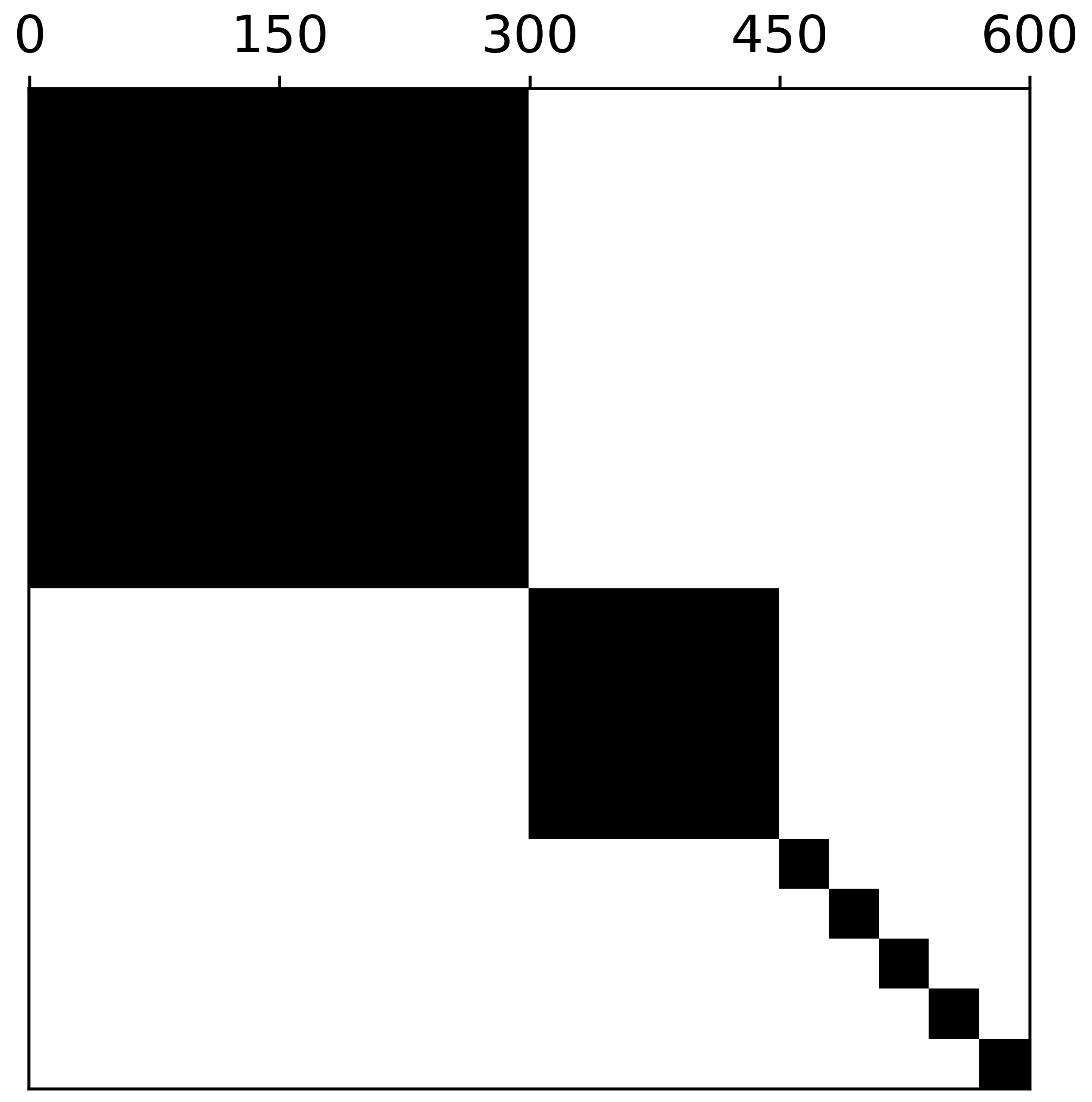
(a) Ground truth $Y^{*}$

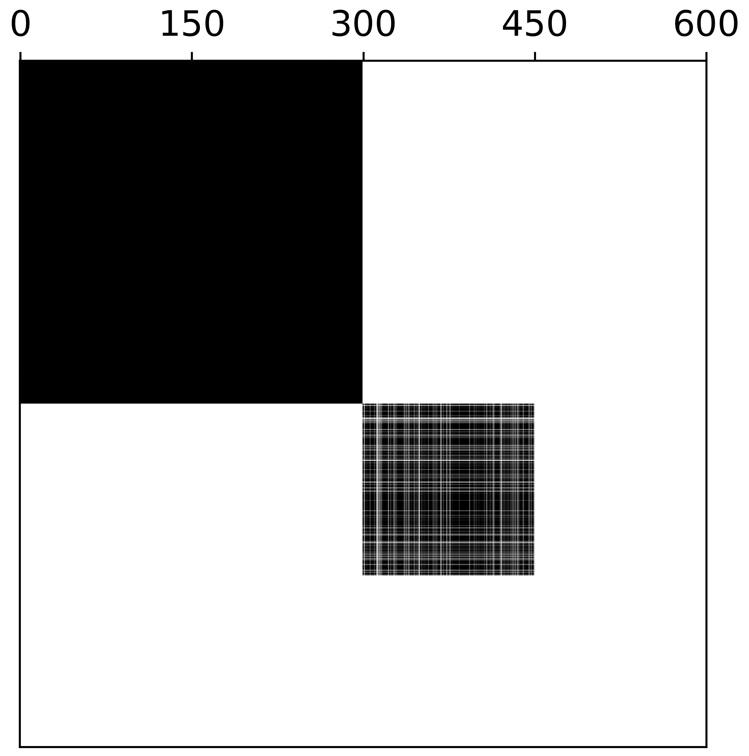
(b) $\widehat{Y}$ with sufficient $\lambda$

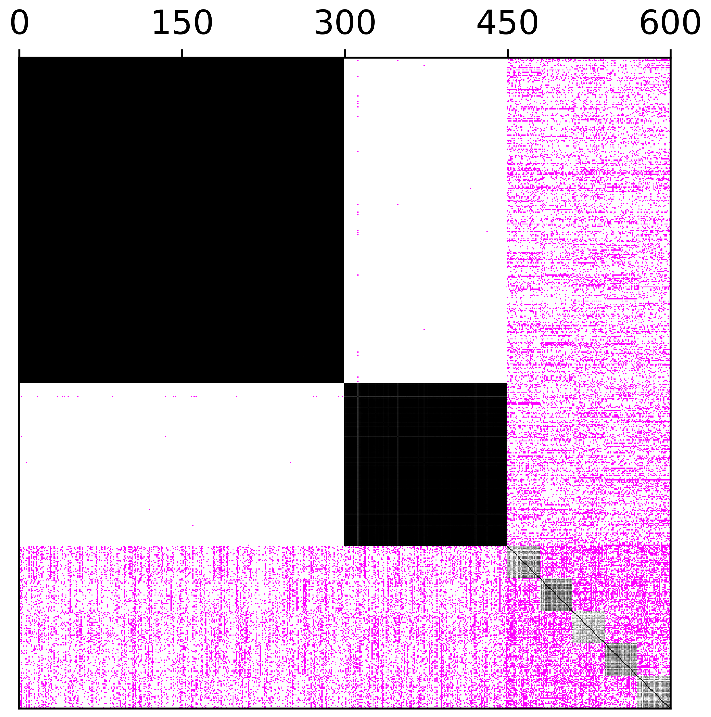
(c) $\widehat{Y}$ with zero or small $\lambda$

Figure 1: SDP solutions and effects of regularization $\lambda$. (a): Ground truth clusters of sizes 300, 150, and 50 ($\times 5$). (b)&(c): Solutions to the SDP (3) with different choices of $\lambda$. Nonzero off-block-diagonal entries are highlighted in pink; other block-diagonal entries shown in grayscale ($\text{white}=0,\text{black}=1$).

2 Our Contributions

We provide a complete resolution of the above question by showing that the recovery SDP (3) returns a desired block-diagonal matrix regardless of the distribution of cluster sizes. Our result completely eliminates the gap assumption, and guarantees recovery of large clusters in the presence of arbitrary middle and small clusters. The middle, critically sized clusters greatly complicate the task of establishing this result. Not only do we no longer have a simple closed form candidate solution for which we can verify optimality, but more significantly, in the presence of threshold-sized clusters the SDP solution $\widehat{Y}$ is extremely sensitive to noise and thus unstable. In particular, as can be seen both numerically and from our analysis, a small perturbation to the graph or cluster sizes may cause a zero block in $\widehat{Y}$ to become near all-one, and vice versa. We overcome these challenges to give a very detailed description of the solution of the SDP, and we believe our most important contributions are the ideas behind this analysis.

Algorithmically, the trace penalty term, which is ignored in most prior work, plays an important role in the recovery SDP (3). This term is not needed when all clusters are large, in which case the hard, entrywise constraint (3c) is sufficient for controlling the diagional entries of $\widehat{Y}$. In the presence of small clusters, however, the trace penalty is essential for ensuring that the SDP solution only captures clusters with sufficient signal and ignores noise, ensuring that we obtain a block-diagonal solution. In Figure 1 we provide an experimental demonstration: Figure 1(c) uses an insufficiently large $\lambda$, and therefore despite finding a solution which is nearly all-one on the two largest clusters, they would still be nontrivial to recover due to the nonzero entries in the off-block-diagonals shown in pink. In contrast, Figure 1(b) shows a solution found with $\lambda$ set sufficiently large so that all off-block-diagonal entries are zero.

We now formally present our main result, which characterizes the solution to the recovery SDP (3) in terms of the solutions to the following oracle SDPs, which are $K$ smaller SDPs of the same form as the recovery SDP except that the full adjacency matrix is replaced by each of the $K$ submatrices corresponding to only the within-cluster edges of each cluster: for $k=1,\dots,K$, let $A^{(k)}=(A_{ij})_{i,j\in V_{k}}\in\mathbb{R}^{s_{k}\times s_{k}}$ and define the $k$th oracle SDP:

$$\widehat{Y}^{k}=\operatorname*{argmax}_{Y\in\mathbb{R}^{s_{k}\times s_{k}}}\quad \left\langle Y,A^{(k)}-\frac{p+q}{2}J_{s_{k}\times s_{k}}\right\rangle-\lambda\operatorname{Tr}(Y)$$ (5a)

s.t. $$Y\succcurlyeq 0,$$ (5b)

$$0\leq Y_{ij}\leq 1,\forall i\in[s_{k}],j\in[s_{k}].$$ (5c)

Of course the formation of the oracle SDPs requires knowledge of the ground-truth clustering $Y^{*}$, so they are only usable for analysis. Now we can state our main theorem.

Theorem 2.

There exist absolute constants $B,\underline{B},\overline{B}>2$ such that the following holds: Fix $m$ such that $m\geq n$ and $p\geq\frac{\log m}{n}$. If we set the regularization parameter $\lambda=\kappa\sqrt{pn\log m}+\delta$ for $\kappa\geq B$ and $\delta\sim\mathrm{Uniform}[0,0.1]$, then with probability at least $1-O(m^{-3})$, the unique solution $\widehat{Y}$ to the recovery SDP (3) is

$$\widehat{Y}=\operatorname{diag}\Big{(}\widehat{Y}^{1},\dots,\widehat{Y}^{K}\Big{)},$$

where $\widehat{Y}^{1},\dots,\widehat{Y}^{K}$ are the unique solutions to the $K$ oracle SDPs (5). Furthermore, for each $k\in\{1,\dots,K\}$, we have $\operatorname{rank}\widehat{Y}^{k}\in\{0,1\}$, and

1. if $\frac{p-q}{2}s_{k}\geq\left(1+\frac{1}{\overline{B}}\right)\kappa\sqrt{pn\log m}$, then $\widehat{Y}^{k}=J_{s_{k}\times s_{k}}=\mathbf{1}\mathbf{1}^{\top}$,

2. if $\frac{p-q}{2}s_{k}\leq\left(1-\frac{1}{\underline{B}}\right)\kappa\sqrt{pn\log m}$, then $\widehat{Y}^{k}=0_{s_{k}\times s_{k}}=00^{\top}$,

3. if $\left(1-\frac{1}{\underline{B}}\right)\kappa\sqrt{pn\log m}<\frac{p-q}{2}s_{k}<\left(1+\frac{1}{\overline{B}}\right)\kappa\sqrt{pn\log m}$, then either $\widehat{Y}^{k}=0$ or $\widehat{Y}^{k}=y^{k}y^{k\top}$ where $y^{k}\geq\frac{1}{2}$ entrywise.

Theorem 2 states that the solution to the recovery SDP will be block-diagonal, and the blocks will match the oracle SDP solutions. We also give a precise characterization of the oracle SDP solutions, which all have rank zero or one, and furthermore are guaranteed to be all-one so long as their cluster size $s_{k}$ satisfies

$$\frac{p-q}{2}s_{k}\geq\left(1+\frac{1}{\overline{B}}\right)\kappa\sqrt{pn\log m}\qquad\text{or equivalently}\qquad\frac{(p-q)^{2}s_{k}^{2}}{pn}\geq B^{\prime}\log m.$$ (6)

Comparing to the gap-dependent condition (4), there is no relative size gap term. With respect to the critically-sized clusters, those satisfying case 3, their oracle solution may be zero, in which case they are not recovered, but whenever the oracle solution is non-zero, it is all-positive, hence recoverable. In the general case where the nodes are not ordered, one can easily postprocess the SDP solution $\widehat{Y}$ to recover the nonzero diagonal blocks promised by the theorem as the off-diagonal blocks are all zero.

Remark 3.

We discuss a few technical points about Theorem 2. First, up to log factors and assuming $p/q=O(1)$, the condition (6) is needed in all known polynomial-time algorithms even when all clusters have the same size (Abbe, 2018; Li et al., 2021; Chen and Xu, 2016). Second, the reason we include an extra parameter $m$ for the failure probability is because we will seek to use Theorem 2 for recursive clustering, which entails removing recovered clusters and then reapplying the clustering procedure to the smaller instance with $n^{\prime}<n$ nodes (which will have a lowered recovery threshold). In this case, we can set $m$ to $n$, the number of nodes in the original problem, instead of $m=n^{\prime}$.

Third, the random perturbation $\delta$ is not practically necessary, but it simplifies the conclusions of the theorem because it guarantees that each of the oracle SDPs (and consequently the recovery SDP) have unique solutions. Without $\delta$, we could have $\lambda_{1}\big{(}\overleftrightarrow{A}^{(k)}\big{)}=\lambda$ for some cluster $k$, which lies exactly on the recovery threshold and causes the $k$th oracle SDP to have non-unique solution; with the perturbation $\delta$ we avoid this boundary situation with probability one. Note that any small perturbation from a continuous distribution would work, and also this only makes any difference for the mid-size clusters in case 3. Finally, the number $(p+q)/2$ used in the SDP (3) can be replaced by other values in the interval $(q,p)$ and thus be treated as a tuning parameter along with $\lambda$. A similar fact is recognized in prior work in the setting where all clusters are big (e.g., Chen et al., 2018; Amini and Levina, 2018).

Now we present the formal version of our gap-dependent recovery result in Theorem 1. While inferior to our main Theorem 2, this result has a simpler proof and is in fact used as a subroutine in the proof of Theorem 2.

Theorem 4.

There exists an absolute constant $C$ such that the following holds: If there exists some $k\in\{1,\ldots,K\}$ such that

$$\frac{p-q}{2}\left(s_{k}-s_{k+1}\right)\geq\kappa\sqrt{pn\log n}\qquad\text{or equivalently}\qquad\frac{(p-q)^{2}\left(s_{k}-s_{k+1}\right)^{2}}{pn}\geq 4\kappa^{2}\log n$$ (7)

and $\kappa\geq C$, then if we set $\lambda=\kappa\sqrt{pn\log n}+\frac{p-q}{2}s_{k+1}$ in (3a), with probability at least $1-O(n^{-3})$,

$$\widehat{Y}=\operatorname{diag}\left(J_{s_{1}\times s_{1}},\dots,J_{s_{k}\times s_{k}},0_{s_{k+1}\times s_{k+1}},\dots,0_{s_{K}\times s_{K}}\right)$$

is the unique optimal solution to the recovery SDP (3).

Note that Theorem 4 also utilizes a value of $\lambda$ which depends on the size of the largest small cluster $s_{k+1}$, which may not be straightforward to find, while Theorem 2 can be set without this information.

Again, we believe our most significant contributions are the ideas behind the proof of Theorem 2. With a more extensive discussion given in the proof sketch in Section 3, here we briefly highlight some key steps. The challenges are mainly associated with the analysis of the oracle SDPs for clusters near the threshold of recovery (case 3 of Theorem 2). The crucial step is to show that the oracle SDP has a rank-one solution, which is the case as long as the non-negativity constraints in (5c) are non-binding. Defining a relaxed oracle SDP by removing these constraints, we reduce the problem to showing that the relaxed oracle SDP solutions are weakly correlated with individual rows of the random noise, suggesting a leave-one-out-style (LOO) argument. However, the naive application of LOO ideas does not work due to the instability of the clusters near the recovery threshold—the removal of one row of noise can drastically change the corresponding SDP solution. To overcome this challenge we define modified LOO versions of the oracle SDPs, relying upon an improved eigenvalue perturbation bound which may be of independent interest and which is discussed below. We hope that some proof techniques may be useful in more generality for problems featuring mixtures of strong and weak signals without a gap between them.

Now we discuss Mukherjee et al. (2022), a contemporary work which also allows the presence of small clusters. Their algorithm, which is based on spectral clustering, also succeeds without the assumption of a gap, recovering clusters meeting conditions almost identical to (6). Both their algorithm and analysis are completely different to our SDP relaxation approach. Our algorithm is conceptually much simpler, and moreover enjoys certain robustness properties against heterogeneous edge probabilities. In comparison, the algorithm in Mukherjee et al. (2022) is quite delicate. We elaborate on this point in Section 2.3.

We next discuss two applications of our result, namely in recursive clustering and the faculty oracle model. In these two settings, our gap-free clustering guarantee exhibits its power, leading to substantial improvements over existing results.

2.1 Recursive Clustering

Theorem 2 demonstrates that we can recover sufficiently large clusters even in the presence of arbitrarily-sized smaller clusters. As first recognized in Ailon et al. (2015), this allows for the use of a recursive clustering procedure: whenever we recover some clusters, we can remove the corresponding nodes from the graph, thereby eliminating some noisy entries and lowering the detection threshold for another application of the recovery procedure. Specifically in our case, recovering more nodes enables us to lower the regularization parameter $\lambda$. We can thus repeatedly apply our clustering algorithm to uncover smaller and smaller clusters, until no more can be found. We emphasize that this recursive clustering procedure operates using only one sample $A$ from the SBM.

To analyze the performance of such a recursive clustering procedure, we follow (Ailon et al., 2015, Theorems 6 and 7) and consider the following setting: $p,q$ are considered fixed and independent of $n$, and $C(p,q)$ is used to denote constants which depend on $p,q$ but not $n$. (Generalization to other settings of $p,q$ is straightforward.) We examine what assumptions on the number of clusters $K$ suffice to ensure that the recursive clustering procedure recovers all but a vanishing fraction of nodes.

Ailon et al. (2015, Theorem 7) roughly states there exists some $C(p,q)$ such that if $K\leq\beta C(p,q)\log n$ for some $\beta\leq 1$, then a recursive clustering procedure will recover clusters containing all but $O(n^{\beta})+O(1)$ nodes. Since, as discussed in Subsection 1.2, their core recovery algorithm requires a certain-sized gap, they require the bound on $K$ to grow at most logarithmically to ensure that a sufficient gap remains after each round.

If we instead apply our gap-free clustering guarantee from Theorem 2, we obtain a significant improvement, allowing $K$ to be polynomially large. In particular, when specialized to the setting above, Theorem 2 guarantees that there exists some $C^{\prime}(p,q)$ such that (with probability $1-O(m^{-3})$) all clusters $k$ satisfying $s_{k}\geq C^{\prime}(p,q)\sqrt{n\log m}$ will be recovered. Using this improved guarantee, we follow the aforementioned recursive clustering strategy to define Algorithm 1. For a square matrix $X$, we use $X_{I}$ to denote the principal submatrix of $X$ indexed by $I$. When the SDP solution $\widehat{Y}$ has the form stated in Theorem 2, each cluster $V_{k}$ corresponding an all-positive block $\widehat{Y}_{V_{k}}$ is said to be recovered.

Algorithm 1 Recursive clustering using Theorem 2

1:$n\times n$ adjacency matrix $A$ sampled from unbalanced SBM

2:Set $n_{1}=n$, $I_{1}=\{1,\ldots,n\}$, round counter $\ell=1$

3:repeat

4:     Recover clusters by applying the SDP (3) to $A_{I_{\ell}}$, where $\lambda$ is set per Theorem 2 with $m=n$

5:     Remove all recovered clusters of size $\geq C^{\prime}(p,q)\sqrt{n_{\ell}\log n}$ from $I_{\ell}$ to obtain $I_{\ell+1}$

6:     Set $n_{\ell+1}=|I_{\ell+1}|$; increase $\ell$ by 1

7:until no clusters are removed

We can prove the following guarantees:

Theorem 5.

Under the above setting, suppose the number of clusters $K$ satisfies $K\leq\frac{n^{\frac{1}{2}-\alpha}}{C^{\prime}(p,q)\sqrt{\log n}}$ for some $0<\alpha<\frac{1}{2}$. Then with probability at least $1-O(n^{-2})$:

1. The algorithm terminates after at most $K$ rounds.

2. Whenever the algorithm terminates, there is at most $n^{1-2\alpha}$ unrecovered nodes remaining.

3. After $\ell$ rounds, there is at most $n^{1-\alpha\sum_{i=0}^{\ell-1}2^{-i}}$ unrecovered nodes remaining.

Note that we interpret an empty summation as zero, that is, $\sum_{\ell=0}^{-1}2^{-\ell}=0$. The algorithm will run for at most $K$ rounds, but it could also be terminated early to save on computation, as part 3 of Theorem 5 guarantees that a large number of nodes will be recovered after only a few rounds. The proof of Theorem 5 is given in Section 6.

2.2 Clustering With a Faulty Oracle

The problem of clustering with a faulty oracle was introduced by Mazumdar and Saha (2017) and has since received significant attention. It can be viewed as an adaptive sampling version of the SBM, where we try to recover clusters by querying $o(n^{2})$ individual entries of the adjacency matrix. Formally, we assume there exist $n$ vertices partitioned into $K$ unknown clusters $V_{1},\dots,V_{K}$ of different sizes. For some bias parameter $\delta>0$, we assume there exists a faulty clustering oracle $\mathcal{O}$ which, upon being queried with a pair of vertices $(i,j)$, returns an answer distributed as

$$\mathcal{O}(i,j)\sim\begin{cases}\text{Bernoulli}(1/2+\delta/2),&\text{if $i,j$ belong to the same cluster},\\ \text{Bernoulli}(1/2-\delta/2),&\text{if $i,j$ do not belong to the same cluster}.\end{cases}$$

These answers are independent for different pairs, and repeating the same query will always produce the same answer.

Clustering with a faulty oracle has several important applications, such as crowdsourced entity resolution and edge prediction in social networks. We refer to Mazumdar and Saha (2017) for more discussion of these applications, and refer to Peng and Zhang (2021) and Mukherjee et al. (2022) for more in-depth comparison of prior work on this problem. We summarize existing algorithms which are computationally efficient and work for general $K$ in Table 1.

Query Complexity	Threshold	Reference	Comments
$O\Big{(}\frac{nK\log n}{\delta^{2}}$ $+\frac{nK^{2}\log n}{\delta^{4}}\wedge\frac{K^{5}\log^{2}n}{\delta^{8}}\Big{)}$	$\Omega\!\left(\frac{K^{4}\log n}{\delta^{2}}\right)$	Mazumdar and Saha (2017)
$O\!\left(\frac{nK\log n}{\delta^{2}}+\frac{K^{4}\log^{2}n}{\delta^{4}}\right)$	$\Omega\!\left(\frac{n}{K}\right)$	Peng and Zhang (2021)	Near-balanced
$O\!\left(\frac{nK\log n}{\delta^{2}}+\frac{K^{10}\log^{2}n}{\delta^{4}}\right)$	$\Omega\!\left(\frac{K^{4}\log n}{\delta^{2}}\right)$	Peng and Zhang (2021)
$O\!\left(\frac{n(K+\log n)}{\delta^{2}}+\frac{K^{8}\log^{3}n}{\delta^{4}}\right)$	$\Omega\!\left(\frac{K^{4}\log n}{\delta^{2}}\right)$	Xia and Huang (2022)
$O\!\left(\frac{nK\log n}{\delta^{2}}\!+\!\frac{K^{9}\log\!K\log^{2}n}{\delta^{12}}\right)$	$\Omega\!\left(\frac{K^{4}\log n}{\delta^{6}}\right)$	Pia et al. (2022)	Semirandom
$O\!\left(\frac{nK\log n}{\delta^{2}}+\frac{K^{5}\log^{2}n}{\delta^{4}}\right)$	$\Omega\!\left(\frac{K^{2}\log n}{\delta^{2}}\right)$	Our Thm. 8
$O\!\left(\frac{n}{s}\frac{n\log n}{\delta^{2}}+\frac{n^{4}}{s^{4}}\frac{\log^{2}n}{\delta^{4}}\right)$	$s$	Mukherjee et al. (2022), Our Thm. 6

Table 1: Comparison of algorithms for clustering with a faulty oracle which are computationally efficient and work for general $K$.

Expanding upon the comments in Table 1, we note that the listed algorithm of Peng and Zhang (2021) assumes that all clusters are “nearly balanced”: they have size at least $\frac{n}{bK}$ for some known constant $b>1$; the algorithm recovers all clusters under this assumption. The algorithm of Pia et al. (2022) is robust to semirandom perturbations (and we refer to their paper for the definition of the semirandom model). As also identified by Mukherjee et al. (2022), all prior algorithms (except that of Mukherjee et al. (2022)) fail when the number of clusters $K$ is large. In particular, $K=\Omega(n^{1/4})$ causes all algorithms in the first 5 rows of Table 1 to have sample complexity $\Omega(n^{2})$ and a recovery threshold size of $\Omega(n)$, with even smaller $K$ still presenting issues for some algorithms.

By utilizing a gap-free clustering subroutine, we can provide an algorithm with a different type of guarantee which circumvents the above issues under large $K$. Letting $s$ be an input parameter, our Algorithm 2 described below (with appropriate parameter setting) can recover all clusters of size at least $s$, and for an appropriate choice of $s$ this leads to an $o(n^{2})$ sample complexity:

Theorem 6.

There exist absolute constants $C_{1},C_{2}$ such that for any parameter $s\geq C_{2}\frac{\sqrt{n\log n}}{\delta}$, by setting $\gamma=C_{2}\frac{n\log n}{s^{2}\delta^{2}}$, with probability at least $1-O(n^{-3})$, Algorithm 2 recovers all clusters of size at least $s$ with query complexity $O\left(\frac{n^{2}}{s}\frac{\log n}{\delta^{2}}+\frac{n^{4}}{s^{4}}\frac{\log^{2}n}{\delta^{4}}\right)$.

We prove Theorem 6 in Section 7. We also note that by setting $s=\frac{n}{K}$ in this result, we recover identical query complexity and cluster recovery threshold to the algorithm of Peng and Zhang (2021) for the nearly-balanced setting listed in Table 1, except our algorithm has no restrictions on cluster sizes as opposed to requiring them to be nearly balanced. Peng and Zhang (2021) conjecture that this sample complexity is optimal among efficient algorithms (up to $\log$ factors) for recovery of clusters of size $\Omega\left(\frac{n}{K}\right)$, based on statistical physics arguments.

Our Algorithm 2 used in Theorem 6 follows a common template for algorithms in the faulty oracle clustering problem:

1. Choose a subset $T$ of the nodes and query all pairs between them.

2. Apply a clustering algorithm on the fully observed subgraph consisting of the nodes $T$ and the edges between them to recover subclusters.

3. Take a subset $S^{\prime}$ from each recovered subcluster of minimal size such that it can be used to test all remaining nodes $i\in[n]\setminus T$ for membership in the cluster, by querying $(i,v)$ for all $v\in S^{\prime}$ and using majority voting.

These essential steps are used in all algorithms in Table 1, with one key difference being the clustering algorithm used in step 2 (for which we use our recovery SDP and Theorem 2). Mukherjee et al. (2022) utilize their (gap-free) spectral clustering procedure and thus obtain a nearly identical result. This template also explains why all the sample complexities (for efficient algorithms) consist of two terms, with the first term roughly corresponding to the majority voting procedure and the second term roughly corresponding to the subsample of size $O(|T|^{2})$, with possible additional steps for some algorithms. Notably, Xia and Huang (2022) improve upon the majority voting procedure by making a connection to best arm identification, obtaining a first term of $\frac{n(K+\log n)}{\delta^{2}}$ which they show is optimal.

Algorithm 2 Clustering with a faulty oracle using Theorem 2

1:Faulty clustering oracle $\mathcal{O}$, parameter $\gamma\in(0,1)$

2:Choose set $T\subseteq[n]$ by including vertex $i$ in $T$ with probability $\gamma$ (independently)

3:Query $(u,v)$ for all pairs $u,v\in T$ to form adjacency matrix $A\in\{0,1\}^{|T|\times|T|}$

4:Recover clusters from $A$ using the recovery SDP (3), where $\lambda$ is set per Theorem 2 with $m=n$

5:for each recovered cluster $S\subseteq T$ such that $|S|\geq\frac{C_{1}\log n}{\delta^{2}}$ do

6:     Choose $S^{\prime}\subseteq S$ with $|S^{\prime}|=\frac{C_{1}\log n}{\delta^{2}}$

7:$\quad\;\;\triangleright$ Recover remainder of cluster in $[n]\setminus T$ by majority voting using $S^{\prime}$ as voters:

8:     for each vertex $i\in[n]\setminus T$ do

9:         Query $(i,v)$ for all $v\in S^{\prime}$ and add $i$ to $S$ if $\frac{1}{|S^{\prime}|}\sum_{v\in S^{\prime}}\mathcal{O}(i,v)\geq\frac{1}{2}$

10:     end for

11:end for

Algorithm 2 requires a user-specified target cluster size $s$, which in turn determines the input parameter $\gamma$, as does (Mukherjee et al., 2022, Algorithm 5). By growing the subsample $T$ geometrically over several rounds, stopping when we first recover a (sub)cluster, we can obtain the following instance-dependent query complexity. Recall that $s_{1}$ is defined to be the largest cluster size.

Theorem 7.

There exist absolute constants $C_{1},C_{2},C_{3}$ such that as long as $s_{1}\geq C_{2}\frac{\sqrt{n\log n}}{\delta}$, with probability at least $1-O(n^{-2})$, Algorithm 3 recovers a cluster of size at least $\frac{s_{1}}{C_{3}}$ with sample complexity $O\left(n\frac{\log n}{\delta^{2}}+\frac{n^{4}}{s_{1}^{4}}\frac{\log^{2}n}{\delta^{4}}\right)$.

We present Algorithm 3 in Section 7 along with the proof of Theorem 7. The strategy of obtaining instance-dependent query complexity using geometric sampling has a crucial reliance on the gap-free recovery guarantee of Theorem 2, since our objective is to sample minimally so that only the largest cluster is recoverable, meaning the recovery procedure must not be sensitive to the presence of slightly smaller but still large clusters. We therefore hope that Theorem 2 lays the foundation for future instance-dependent algorithms for clustering with a faulty oracle.

Even in the setting where $K$ is small, by using our Theorem 2 instead of clustering subroutines which require the existence of cluster size gaps, we can obtain the following result which makes improvements to previous query complexities and recovery thresholds, while also having a substantially simpler algorithm and proof.

Theorem 8.

With probability at least $1-O(n^{-2})$, Algorithm 4 recovers all clusters of size at least $\Omega\left(\frac{K^{2}\log n}{\delta^{2}}\right)$ with query complexity $O\left(\frac{nK\log n}{\delta^{2}}+\frac{K^{5}\log^{2}n}{\delta^{4}}\right)$.

The Algorithm 4 used above, which we provide in Section 7 along with the proof of Theorem 8, is nearly identical to Algorithm 2 except we use a different subsampling ratio $\gamma$ and repeat in at most $K$ rounds (choosing a new subsample $T$ each round). This use of $K$ rounds is the reason that the second term in the query complexity is $\frac{K^{5}\log^{2}n}{\delta^{4}}$ rather than the $\frac{K^{4}\log^{2}n}{\delta^{4}}$, which Peng and Zhang (2021) conjecture is optimal for the nearly balanced setting. In the setting that all clusters are $\Omega\left(\frac{n}{K}\right)$, only one round of choosing $T\subseteq[n]$ and querying all pairs $u,v\in T$ would be needed to recover a subcluster from each of the $K$ clusters, while in general settings more rounds have the potential benefit of recovering smaller clusters after larger clusters are removed. (In fact, our Algorithm 4 would match this conjectured-optimal sample complexity in the nearly-balanced setting as it would terminate after a constant number of rounds.) In summary, our algorithm recovers smaller clusters and improves upon the second term in the sample complexity compared to all previous algorithms which work for the case of general size clusters. We also believe that the first term could be improved to $\frac{n(K+\log n)}{\delta^{2}}$ using ideas from Xia and Huang (2022), but our focus was on the improvement available by using a gap-free clustering subroutine.

2.3 Heterogeneous Connectivity Probabilities

We return to the Stochastic Block Model, but now consider a more general heterogenous setting. Again let $[n]$ be a set of vertices partitioned into $K$ unknown clusters of sizes $V_{1},\dots,V_{K}$, and $A\in\{0,1\}^{n\times n}$ the observed adjacency matrix. However, now we further suppose that for each $i,j\in[n]$ such that $i$ and $j$ are members of distinct clusters, there exist numbers $q_{ij}=q_{ji}$ such that $1\geq p>q\geq q_{ij}\geq 0$, and that $A$ is sampled such that independently across all $i\leq j$,

$$A_{ij}\sim\begin{cases}\text{Bernoulli}(p),&\text{if $i,j$ belong to the same cluster},\\ \text{Bernoulli}(q_{ij}),&\text{if $i,j$ do not belong to the same cluster}.\end{cases}$$

Thus, whereas we previously considered all $q_{ij}=q$, now we allow the between-cluster edge probabilities $q_{ij}$ to depend on the two nodes $i,j$ so long as the bounds $q_{ij}\leq q$ hold. We refer to this setting as the heterogeneous inter-connectivity SBM. Despite seemingly easing the clustering task, the heterogeneous model can disrupt many local structures of the SBM, foiling algorithms dependent on such structures. For instance, when the $q_{ij}$’s were homogeneous, the expected degree of a node $i$ in cluster $k$ would satisfy the identity $\sum_{j\in[n]}\mathbb{E}A_{ij}=ps_{k}+q(n-s_{k})$, in which case the observed degree of node $i$ can be used to estimate the cluster size $s_{k}$. The algorithm of Mukherjee et al. (2022) utilizes such a subroutine for estimating the largest cluster size. Under the heterogeneous inter-connectivity SBM, such procedures would not directly work.

In contrast, the SDP (3) and our same Theorem 2 continue to work:

Theorem 9.

Under the above heterogeneous inter-connectivity SBM, the conclusions from Theorem 2 hold.

We present the proof of Theorem 9 in Section 8, but it is trivial as nearly every word of the proof of Theorem 2 is still true. Similar phenomena, that many proofs for the SDP relaxation approach generalize (often automatically) to heterogeneous or even semi-random generative models, have been observed in the literature and recognized as a testament of the robustness of the SDP approach; see Moitra et al. (2016); Amini and Levina (2018) and the references therein. The situation is somewhat more subtle in the presence of unbalanced clusters: while proving Theorem 9 is straightforward, further generalizing to heterogeneous intra-connectivity probabilities $p_{ij}$’s is more challenging due to the instability of solution blocks of the mid-sized clusters. We believe such generalization is possible but may necessitate alternative choices of the trace regularization parameter $\lambda$ and the centering parameter $(p+q)/2$ (cf. Remark 3)—we leave this to future work. As such, we treat Theorem 9 as an important step in developing robust algorithms for unbalanced community detection.

2.4 Eigenvalue Perturbation Bounds

As elaborated in the proof sketch in Section 3, to circumvent the instability inherent to the threshold-size cluster oracle SDP solutions, we modify standard leave-one-out techniques by also changing the regularization strength. This requires eigenvalue perturbation bounds which improve upon existing results.

We provide some brief background on related eigenvalue perturbation results and refer to Eldridge et al. (2018) for more details. Let $M,H\in\mathbb{R}^{n\times n}$ be symmetric matrices, viewing $H$ as a perturbation, and let $v_{1}$ be a top eigenvector of $M$. If we would like to bound $\left|\lambda_{1}(M+H)-\lambda_{1}(M)\right|$, the classical Weyl’s inequality gives that

$$\left|\lambda_{1}(M+H)-\lambda_{1}(M)\right|\leq\left\|H\right\|_{\textnormal{op}}.$$

As argued in Eldridge et al. (2018), this bound can be overly pessimistic, especially when $H$ is a random perturbation whose projection onto $v_{1}$ is small relative to the eigengap $\lambda_{1}(M)-\lambda_{2}(M)$. In such a situation, intuitively the large eigengap should ensure that the new top eigenvector of $M+H$ is close to $v_{1}$, in which case the top eigenvalue of $M+H$ will be approximately $v_{1}^{\top}\left(M+H\right)v_{1}=\lambda_{1}(M)+v_{1}^{\top}Hv_{1}$, and then since $H$ is random, $\left|v_{1}^{\top}Hv_{1}\right|$ should be much smaller than $\left\|H\right\|_{\textnormal{op}}$. The idea that $\left|\lambda_{1}(M+H)-\lambda_{1}(M)\right|\approx\left|v_{1}^{\top}Hv_{1}\right|$ is stated as an informal guiding principle in Eldridge et al. (2018), and they confirm the above intuition with both experiments and theoretical results. Let $\operatorname{Col}Q$ denotes the span of the columns of a matrix $Q$. They prove the following upper bound:

Theorem 10 (Eldridge et al. (2018), Theorem 6).

Let $T\in[n]$ and $h$ be such that $|x^{\top}Hx|\leq h$ for all $x\in\operatorname{Col}(U_{1:T})$ with $\left\|x\right\|_{2}=1$, where $U_{1:T}$ are the top $T$ eigenvectors of $M$. Then for $t\leq T$, if $\lambda_{t}-\lambda_{T+1}>2\left\|H\right\|_{\textnormal{op}}-h$,

$$\lambda_{t}(M+H)\leq\lambda_{t}(M)+h+\frac{\left\|H\right\|_{\textnormal{op}}^{2}}{\lambda_{t}(M)-\lambda_{T+1}(M)+h-\left\|H\right\|_{\textnormal{op}}}.$$

We modify their argument to prove the following improvement:

Theorem 11.

Let $T\in[n]$ and $h$ be such that $|x^{\top}Hx|\leq h$ for all $x\in\textnormal{Col}(U_{t:T})$ with $\left\|x\right\|_{2}=1$, where $U_{t:T}$ are eigenvectors $t$ through $T$ of $M$. Then for $t\leq T$, if $\lambda_{t}-\lambda_{T+1}>\left\|H\right\|_{\textnormal{op}}-h-2\left\|HU_{t:T}\right\|_{\textnormal{op}}$,

$$\lambda_{t}(M+H)\leq\lambda_{t}(M)+h+\frac{\left\|HU_{t:T}\right\|_{\textnormal{op}}^{2}}{\lambda_{t}(M)-\lambda_{T+1}(M)-\left\|H\right\|_{\textnormal{op}}+h+2\left\|HU_{t:T}\right\|_{\textnormal{op}}}.$$

We prove Theorem 11 in Section 9. Notice that compared to Theorem 10, Theorem 11 has slightly weakened assumptions, and always provides a better bound since $\left\|HU_{t:T}\right\|_{\textnormal{op}}\leq\left\|H\right\|_{\textnormal{op}}$. Especially when $H$ is random and $T$ is small, $\operatorname{Col}(U_{t:T})$ is a small subspace and so we might hope that $\left\|HU_{t:T}\right\|_{\textnormal{op}}\ll\left\|H\right\|_{\textnormal{op}}$.

Now we compare these results within the context of the proof of Theorem 2, and show that the improvement from our Theorem 11 is indeed substantial. In this subsection we also write $a_{n}\asymp b_{n}$ if $a_{n}\lesssim b_{n}$ and $b_{n}\lesssim a_{n}$. Fix a cluster $k$ so that $\frac{p-q}{2}s_{k}\asymp\kappa\sqrt{pn\log n}$. Let $w^{\top}$ be the first row of $W^{(k)}$ except with its first entry halved. This is chosen so that by defining $H=e_{1}w^{\top}+we_{1}^{\top}$, $H$ contains the noise from the first row and column of $W^{(k)}$. Now let $M=\overleftrightarrow{A}^{(k)}-H$ (so $M+H=\overleftrightarrow{A}^{(k)}$). Our objective will be to bound $\left|\lambda_{1}\left(\overleftrightarrow{A}^{(k)}\right)-\lambda_{1}\left(\overleftrightarrow{A}^{(k)}-H\right)\right|$. By the assumption on the size of the cluster $k$, there is sufficient signal so that the top eigenvector $v_{1}$ of $M$ satisfies $\left\|v_{1}\right\|_{\infty}\lesssim\frac{1}{\sqrt{s_{k}}}$ (by applying an $\infty$-norm eigenvector perturbation bound (Chen et al., 2021)). Then

$$\left|v_{1}^{\top}Hv_{1}\right|=2|v_{1}^{\top}e_{1}||w^{\top}v_{1}|\lesssim\frac{1}{\sqrt{s_{k}}}\sqrt{p\log n}$$

where the bound $|w^{\top}v_{1}|\lesssim\sqrt{p\log n}$ holds with high probability using the fact that $w$ is independent from $v_{1}$ (since $v_{1}$ is the top eigenvector of a matrix where the first row and column of noise have been set to $0$). The informal guiding principle from Eldridge et al. (2018) would then give us hope that $\left|\lambda_{1}\left(\overleftrightarrow{A}^{(k)}\right)-\lambda_{1}\left(\overleftrightarrow{A}^{(k)}-H\right)\right|\lesssim\frac{\sqrt{p\log n}}{\sqrt{s_{k}}}$, which is the order needed within our proof of Theorem 2. Unfortunately, Theorem 10 only yields that

$$\lambda_{1}\left(\overleftrightarrow{A}^{(k)}\right)-\lambda_{1}\left(\overleftrightarrow{A}^{(k)}-H\right)\lesssim\frac{\sqrt{p\log n}}{\sqrt{s_{k}}}+\frac{\left\|H\right\|_{\textnormal{op}}^{2}}{\kappa\sqrt{pn\log n}-\left\|H\right\|_{\textnormal{op}}}\lesssim\frac{\left(\sqrt{ps_{k}}\right)^{2}}{\kappa\sqrt{pn\log n}}\lesssim\frac{\sqrt{p}s_{k}}{\kappa\sqrt{n\log n}}$$

since $\left\|H\right\|_{\textnormal{op}}\asymp\left\|w\right\|_{2}\asymp\sqrt{ps_{k}}$. However, since

$$\left\|Hv_{1}\right\|_{\textnormal{op}}=\left\|we_{1}^{\top}v_{1}+e_{1}w^{\top}v_{1}\right\|_{2}\leq\left\|w\right\|_{2}\left|e_{1}^{\top}v_{1}\right|+\left|w^{\top}v_{1}\right|\lesssim\sqrt{ps_{k}}\frac{1}{\sqrt{s_{k}}}+\sqrt{p\log n}\lesssim\sqrt{p\log n}$$

our Theorem 11 gives that

$$\lambda_{1}\left(\overleftrightarrow{A}^{(k)}\right)-\lambda_{1}\left(\overleftrightarrow{A}^{(k)}-H\right)\lesssim\frac{\sqrt{p\log n}}{\sqrt{s_{k}}}+\frac{\left(\sqrt{p\log n}\right)^{2}}{\kappa\sqrt{pn\log n}}\lesssim\frac{\sqrt{p\log n}}{\sqrt{s_{k}}}+\frac{\sqrt{p\log n}}{\kappa\sqrt{n}}\lesssim\frac{\sqrt{p\log n}}{\sqrt{s_{k}}}.$$

2.5 Additional Related Work

In proceeding sections we have provided references to SBM algorithms focusing on SDP relaxation and spectral clustering methods. There are many other approaches, such as the EM algorithm (Snijders and Nowicki, 1997) and local search methods (Carson and Impagliazzo, 2001; Jerrum and Sorkin, 1998), many of which may be coupled with an SDP-based or spectral algorithm with the latter serving as an initialization procedure (Lu and Zhou, 2016; Vu, 2018; Abbe, 2018).

Many works have considered the setting that all clusters are sufficiently large to be exactly recovered, leading to precise computational and information-theoretic thresholds in the case of two balanced clusters (Abbe et al., 2015; Mossel et al., 2015a). Much subsequent work has endeavored to obtain similar characterizations in more general settings, for instance in Abbe and Sandon (2015), Abbe et al. (2017), Perry and Wein (2017), Agarwal et al. (2017), and Jog and Loh (2015), where typical recovery conditions have the form $\frac{(p-q)^{2}}{pn}s_{K}\gtrsim\log n$ assuming $p,q\asymp\frac{\log n}{n}$, where $s_{K}$ is the size of the smallest cluster. There is also a complementary weak or approximate recovery setting, where the objective is to achieve strictly better classification error than random guess, usually under the constant degree regime $p,q\asymp\frac{1}{n}$. Again precise phase transitions have been established for the two-balanced-clusters case (Massoulié, 2014; Lelarge et al., 2015; Mossel et al., 2015b), and generalizations to larger $K$ or unbalanced settings, such as Bordenave et al. (2015), Coja-Oghlan et al. (2017), Caltagirone et al. (2017), and Montanari and Sen (2016), develop recovery conditions of the form $\frac{(p-q)^{2}}{pn}s_{K}\gtrsim 1$. While the focus of the current paper is mostly orthogonal to the above work, our result, when specialized to the setting where all clusters are large, recovers the the condition $\frac{(p-q)^{2}}{pn}s_{K}\gtrsim\log n$ typical in existing work.

Our discussion on the heterogeneous setting is related to a line of work on the more general semi-random SBM (Moitra et al., 2016; Krivelevich and Vilenchik, 2006; Feige and Kilian, 2001). In particular, any recovery result for semi-random SBM implies a result for SBM with heterogeneous edge probabilities via a standard reduction (Chen et al., 2014). Generalizaing our results to semi-random SBM is an interesting future direction.

For more on the leave-one-out approach applied to clustering and related matrix estimation problems, see Zhong and Boumal (2018); Abbe et al. (2020); Ding and Chen (2020), as well as the survey in Chen et al. (2021). The work Green Larsen et al. (2020) study faulty oracle clustering in the setting of $K=2$ clusters.

2.6 Notation

For any $n\times n$ matrix $M$, we let $M^{(i)}$ denote the $s_{i}\times s_{i}$ principal submatrix of $M$ obtained by deleting all rows and columns not associated with cluster $i$. We define $M^{(ij)}$ to be the $s_{i}\times s_{j}$ submatrix obtained by deleting all rows not associated with cluster $i$ and all columns not associated with cluster $j$. We also use this notation for vectors: if $v\in\mathbb{R}^{n}$, we define $v^{(i)}$ to be the vector of length $s_{i}$ obtained by deleting all entries not associated with cluster $i$. We use $M_{ij}$ to denote the $(i,j)$th entry of $M$ and $v_{i}$ to denote the $i$th entry of $v$. In the case both notations are present we define the block indexing to bind first, so for example $v^{(i)}_{j}=(v^{(i)})_{j}$.

We use $\left\langle X,Y\right\rangle:=\sum_{ij}X_{ij}Y_{ij}$ to denote the matrix inner product, and $X\circ Y$ the element-wise product between two matrices $X$ and $Y$. We also use the following matrix norms: $\left\|X\right\|_{\textnormal{op}}$ is the largest singular value of $X$, $\left\|X\right\|_{\textnormal{nuc}}$ is the sum of singular values of $X$, $\left\|X\right\|_{1}:=\sum_{i,j}\left|X_{ij}\right|$, and $\left\|X\right\|_{\infty}:=\max_{i,j}\left|X_{ij}\right|$. We define the support of a matrix $\text{supp}(X):=\left\{(i,j):X_{ij}\neq 0\right\}$. We for square matrices $M_{1}\in\mathbb{R}^{m_{1}\times m_{1}},\dots,M_{r}\in\mathbb{R}^{m_{r}\times m_{r}}$, we use the notation $\operatorname{diag}\left(M_{1},\dots,M_{m}\right)$ to denote a $(\sum_{i=1}^{r}m_{r})\times(\sum_{i=1}^{r}m_{r})$ block-diagonal matrix with diagonal blocks $M_{1},\dots,M_{r}$.

We denote by $J_{n_{1}\times n_{2}}$ the $n_{1}\times n_{2}$ all-one matrix, and we sometimes drop the subscripts when the size is clear from context. We also use $\mathbf{1}_{m}$ to denote a length-$m$ vector of all ones, again occasionally dropping subscripts. We define $\overline{e}=\mathbf{1}/\left\|\mathbf{1}\right\|_{2}$ and we let $e_{j}$ denote a standard basis vector with entry $j$, both of which are only used when their size is clear from context. For any event $E$ we define $E^{c}$ to be its complement. For any natural number $h$ we define $[h]=\{1,\dots,h\}$.

2.7 Organization of the Remainder of the Paper

We provide a proof sketch outlining our main analytical insights in Section 3. We formally prove the main Theorem 2 in Section 4. The proof is split into two main parts, on the behavior of the oracle SDPs in Subsection 4.1, and on the recovery SDP solution in Subsection 4.2. The gap-dependent recovery result Theorem 4, a version of which is used in the proof of Theorem 2, is proven in Subsection 4.3, and several concentration results used for these proofs are collected in Subsection 4.4. Section 5 contains discussion of further research directions. We provide a proof for our recursive clustering result in Section 6, and we present algorithms and proofs for faulty oracle clustering in Section 7. We describe how to extend our main theorem to the heterogeneous inter-connectivity setting in Section 8. We prove our eigenvalue perturbation bounds in Section 9.

3 Proof Outline of Main Theorem

In this section, we discuss the high-level approach of the proof of Theorem 2. The general strategy is to construct a candidate primal solution to the recovery SDP (3) as well as dual variables which certify its optimality by satisfying the KKT conditions—this is known as the primal-dual witness approach (Wainwright, 2019; Cai and Li, 2015). The construction relies on establishing that the oracle SDPs (5) have rank-one and “well-spread” solutions, which is most challenging for the oracle blocks corresponding to the mid-size clusters. To handle this case, we first observe that if the lower-bound constraints $\widehat{Y}^{k}\geq 0$ are non-binding (in the sense that their removal does not change the solution), then the $k$th oracle SDP must have a rank $\leq 1$ solution. As we argue in Subsection 3.2.2 below, showing that these constraints are non-binding is closely related to controlling the correlation between the oracle SDP solution and each row of the $k$th oracle noise matrix $W^{(k)}$. This suggests a leave-one-out-style argument, where the correlation strength is quantified by the change of the solution when a row of $W^{(k)}$ is left out. However, due to the arbitrary proximity of the mid-size clusters to the recovery boundary, if we define an auxiliary SDP with one row and column of noise zeroed-out (similar to previous works such as Zhong and Boumal (2018)), it may have a drastically different solution. To remedy this issue, we go beyond modifying one row of noise and also modify the regularization strength. The correct modification of the regularization strength requires improved eigenvalue perturbation bounds in order to ensure that the leave-one-out solution and the oracle SDP solution are suitably close.

Recall we write we write $a_{n}\lesssim b_{n}$ if $a_{n}\leq Cb_{n},\forall n$ for a universal constant $C>0$ and $a_{n}\asymp b_{n}$ if $a_{n}\lesssim b_{n}$ and $b_{n}\lesssim a_{n}$. In this sketch we will simply set $m=n$. Our regularization parameter $\lambda$ will be at least $\kappa\sqrt{pn\log n}$ for some $\kappa$ which is a fixed absolute constant which we can make arbitrarily large. We will write $\varepsilon$ in place of terms which are $\asymp\frac{1}{\kappa}$, which may be multiple (unequal) terms in the same expression.

3.1 Setting up primal-dual witness argument

Our goal is to show the solution is block-diagonal with support contained within that of the ground truth $Y^{*}$, and also we do not have closed-form expressions for each block (since the mid-size blocks are highly sensitive to the particular instantiation of the noise). These two considerations motivate us to consider the $K$ oracle SDPs (5) associated with each cluster and combine their respective solutions $\widehat{Y}^{1},\dots,\widehat{Y}^{K}$ to form our candidate solution $\widehat{Y}=\operatorname{diag}\left(\widehat{Y}^{1},\dots,\widehat{Y}^{K}\right)$. Equivalently, this strategy can be viewed as finding a solution to the recovery SDP which is constrained to be block-diagonal.

Thus $\widehat{Y}$ is the optimal solution of the recovery SDP if we can find dual variables $U,L\in\mathbb{R}^{n\times n}$ such that

$$U,L\geq 0$$ (8a)

$$U\circ\left(\widehat{Y}-J_{n\times n}\right)=L\circ\widehat{Y}=0_{n\times n}$$ (8b)

$$\overleftrightarrow{A}-\lambda I-U+L\preccurlyeq 0_{n\times n}$$ (8c)

$$\left(\overleftrightarrow{A}-\lambda I-U+L\right)\widehat{Y}=0_{n\times n}.$$ (8d)

A powerful feature of the oracle strategy is that each oracle SDP solution must satisfy its own similar KKT conditions: for each $k\in[K]$, there exist dual variables $U^{k},L^{k}\in\mathbb{R}^{s_{k}\times s_{k}}$ such that

$$U^{k},L^{k}\geq 0$$ (9a)

$$U^{k}\circ\left(\widehat{Y}^{k}-J_{s_{k}\times s_{k}}\right)=L^{k}\circ\widehat{Y}^{k}=0_{s_{k}\times s_{k}}$$ (9b)

$$\overleftrightarrow{A}^{(k)}-\lambda I-U^{k}+L^{k}\preccurlyeq 0_{s_{k}\times s_{k}}$$ (9c)

$$\left(\overleftrightarrow{A}^{(k)}-\lambda I-U^{k}+L^{k}\right)\widehat{Y}^{k}=0_{s_{k}\times s_{k}}.$$ (9d)

The oracle conditions (9) are nearly sufficient to be reassembled to find a solution for the recovery conditions (8) (by setting $U=\operatorname{diag}(U^{1},\dots,U^{k})$), but we are left with a choice for how to set the non-block-diagonal entries of $L$. This choice cannot be made without first gaining more detailed information about the oracle solutions $\widehat{Y}^{k}$, particularly that they are rank-one and “well-spread.” The reasons will be made more clear once we fully construct $L$, but for now we can motivate these requirements with the following observations: Suppose for simplicity that $K=2$. The condition (9d) guarantees that each nontrivial eigenvector $v\in\mathbb{R}^{s_{1}}$ of $\widehat{Y}^{1}$ will satisfy $\left(\overleftrightarrow{A}^{(1)}-U^{1}+L^{1}\right)v=\lambda v$. Now letting $\overline{v}\in\mathbb{R}^{n}$ be a zero-padded version of $v$ such that $\overline{v}^{(1)}=v$, we will have

$$\left(\overleftrightarrow{A}-U+L\right)\overline{v}=\begin{bmatrix}\overleftrightarrow{A}^{(1)}-U^{1}+L^{1}&\overleftrightarrow{A}^{(12)}+L^{(12)}\\ \overleftrightarrow{A}^{(21)}+L^{(21)}&\overleftrightarrow{A}^{(2)}-U^{2}+L^{2}\end{bmatrix}\begin{bmatrix}v\\ 0\end{bmatrix}=\begin{bmatrix}\lambda v\\ \left(\overleftrightarrow{A}^{(21)}+L^{(21)}\right)v\end{bmatrix}.$$ (10)

This vector has norm at least $\lambda$, so the only way not to violate (8c) is for $\left(\overleftrightarrow{A}^{(21)}+L^{(21)}\right)v=0$. Therefore, each eigenvector (corresponding to a nonzero eigenvalue) of $\widehat{Y}^{1}$ places a requirement on the form of $L^{(21)}$, and in order for the entries of $\overleftrightarrow{A}^{(21)}v=\left(-\frac{p-q}{2}J_{s_{2}\times s_{1}}+W^{(21)}\right)v$ to concentrate around $-\frac{p-q}{2}$ so that we may choose $L^{(21)}\geq 0$, we will need $\left\|v\right\|_{\infty}$ to be sufficiently small.

3.2 Analyzing oracle SDPs

Now we can discuss how to establish these facts about the oracle SDPs. Fix a cluster $k$. If the signal $\frac{p-q}{2}s_{k}$ is sufficiently small or large, everything is relatively simple. If $\frac{p-q}{2}s_{k}\leq(1-\varepsilon)\lambda$, then the top eigenvalue of $\overleftrightarrow{A}-\lambda I$ will be negative, so $\widehat{Y}^{k}$ will be zero. If $\frac{p-q}{2}s_{k}\geq(1+\varepsilon)\lambda$, then we can essentially apply the gap-dependent recovery Theorem 4 to guarantee that $\widehat{Y}^{k}=J_{s_{k}\times s_{k}}$ (since, with only one cluster, we need not worry about smaller clusters being sufficiently small). This leaves the most interesting mid-size case, where $\frac{p-q}{2}s_{k}$ is within a small multiple of $\lambda$.

3.2.1 Showing relaxed oracle SDP has rank-one solution

In this situation, there is no closed-form candidate for $\widehat{Y}^{k}$ independent of the realization of $A$; entries may be neither 0 nor 1. Experimentally, when $\lambda$ is sufficiently large, the oracle solutions have no zero entries (unless the entire block is zero), meaning the non-negativity constraints are non-binding. Removing these constraints gives the simpler relaxed oracle SDP:

$$\overline{Y}^{k}=\operatorname*{argmax}_{Y\in\mathbb{R}^{s_{k}\times s_{k}}}\quad \left\langle Y,A^{(k)}-\frac{p+q}{2}J_{s_{k}\times s_{k}}\right\rangle-\lambda\operatorname{Tr}(Y)$$ (11a)

s.t. $$Y\succcurlyeq 0,$$ (11b)

$$Y_{ii}\leq 1,\forall i\in[s_{k}].$$ (11c)

A key simplification in the relaxed oracle SDP is that the KKT conditions (9c) and  (9d) become

$$\overleftrightarrow{A}^{(k)}-\lambda I-\operatorname{diag}(u^{k})\preccurlyeq 0_{s_{k}\times s_{k}}$$ (12a)

$$\left(\overleftrightarrow{A}^{(k)}-\lambda I-\operatorname{diag}(u^{k})\right)\overline{Y}^{k}=0_{s_{k}\times s_{k}}.$$ (12b)

Since $\overleftrightarrow{A}^{(k)}=\frac{p-q}{2}J+W^{(k)}$, that is a noisy perturbation of a rank-one matrix, and also since $\operatorname{diag}(\overline{u}^{k})\succcurlyeq 0$, if $\lambda>\left\|W^{(k)}\right\|_{\textnormal{op}}$ then we will be guaranteed that $\overleftrightarrow{A}^{(k)}-\lambda I-\operatorname{diag}(\overline{u}^{k})$ has all eigenvalues strictly negative except for at most one (which by (12a) must then be equal to zero). Thus we can combine this with the fact that $\overline{Y}^{k}\succcurlyeq 0_{s_{k}\times s_{k}}$ and (12b) to conclude that $\overline{Y}^{k}$ must have rank zero or one. Thus we can write $\overline{Y}^{k}=yy^{\top}$ (choosing the sign of $y$ so that $\mathbf{1}^{\top}y\geq 0$). We note that this step is somewhat related to Sagnol (2011) which shows a similarly structured SDP has low-rank solution, but Sagnol (2011) assumes that the objective matrix is low-rank, while we instead use the fact that it has a low number of positive eigenvalues.

3.2.2 Setting up leave-one-out technique to control noise correlation

To justify our use of the relaxed oracle SDP, we must show that $\overline{Y}^{k}$ or equivalently $y$ are elementwise-non-negative, in which case the relaxed oracle SDP solution will also be feasible for the oracle SDP, and therefore the optimal solution for the oracle SDP will be $\overline{Y}^{k}=yy^{\top}$. This is easy to check when $\lambda_{1}\left(\overleftrightarrow{A}^{(k)}\right)<\lambda$, since in this case $\overline{Y}^{k}=0_{s_{k}\times s_{k}}$, so we can focus on the case where $\lambda_{1}\left(\overleftrightarrow{A}^{(k)}\right)>\lambda$ and $\overline{Y}^{k}$ is nonzero. Now we argue why this reduces to bounding the correlation between $y$ and the rows of the noise matrix $W^{(k)}$.

Since the argument is identical for all entries, we focus on showing that $y_{1}\geq 0$. By using the fact that $\overline{Y}^{k}$ is rank-one and rearranging the optimality condition (12b), we obtain

$$y_{1}=\frac{1}{\lambda}\left(\frac{p-q}{2}\mathbf{1}^{\top}y+w^{\top}y-u^{k}_{1}y_{1}\right),$$

where $w^{\top}$ is the first row of $W^{(k)}$. If $y_{1}=1$ then we are done, and otherwise either $y_{1}\in(-1,1)$ so $u_{1}^{k}=0$, or $y_{1}=-1$ and then $-u^{k}_{1}y_{1}\geq 0$. Thus

$$y_{1}\geq\frac{1}{\lambda}\left(\frac{p-q}{2}\mathbf{1}^{\top}y+w^{\top}y\right).$$ (13)

Since in a mid-size cluster $(1-\varepsilon)\lambda\leq\frac{p-q}{2}s_{k}\leq(1+\varepsilon)\lambda$, and it is straightforward to show $\mathbf{1}^{\top}y\geq s(1-\varepsilon)$, the first term on the RHS is close to one. Therefore it suffices to show that $w$ and $y$ are uncorrelated, specifically that $\left|w^{\top}y\right|\lesssim\varepsilon\lambda$.

The entries of $w$ are bounded by $1$ and each have variance $\leq p$, while $y$ has $\left\|y\right\|_{2}\leq\sqrt{s_{k}}$ and $\left\|y\right\|_{\infty}\leq 1$, so if they were independent we could apply Bernstein’s inequality to conclude $\left|w^{\top}y\right|\lesssim\sqrt{ps_{k}\log n}\leq\varepsilon\lambda$. The challenge is that they are not independent. Furthermore, naively bounding $\left|w^{\top}y\right|\leq\left\|w\right\|_{2}\left\|y\right\|_{2}\lesssim(\sqrt{ps_{k}})(\sqrt{s_{k}})$ does not work, because this bound can be much larger than $\lambda=\kappa\sqrt{pn\log n}$. Still, the guiding intuition is that since $y$ needs to depend on all rows of $W^{(k)}$, it should not be strongly correlated with any single row. This is the standard motivation for the leave-one-out technique: to formalize this intuition, we can form a LOO relaxed oracle SDP where we set the noise in the first row and column of $\overleftrightarrow{A}^{(k)}$ to zero, and let its solution (which is also rank-one) be $\widetilde{y}\widetilde{y}^{\top}$. Then $\widetilde{y}$ will be independent of $w$, but we might hope it will also be very close to $y$, two facts which we could combine to show $|w^{\top}y|\approx|w^{\top}\widetilde{y}|\lesssim\sqrt{ps_{k}\log n}$.

Due to the extreme noise sensitivity inherent to the mid-size clusters, this strategy will not work: after leaving out noise to get $\widetilde{A}$, we may have $\lambda_{1}\left(\widetilde{A}\right)<\lambda$ (even though $\lambda_{1}\left(\overleftrightarrow{A}^{(k)}\right)>\lambda$), which means we will have solution $\widetilde{y}\widetilde{y}^{\top}=0_{s_{k}\times s_{k}}$ for the LOO relaxed oracle SDP. In simpler terms, the usual LOO solution $\widetilde{y}$ might be very different from $y$. To overcome this issue, we will also reduce the regularization parameter $\lambda$ used for the LOO problem, to a value $\widetilde{\lambda}$ which is just small enough to guarantee that $\lambda_{1}\left(\widetilde{A}\right)>\widetilde{\lambda}$. Of course, if $\widetilde{\lambda}$ is too small then $\widetilde{y}$ might be significantly different from $y$. Existing eigenvalue perturbation bounds from (Eldridge et al., 2018, Theorem 6) are too large to use in our remaining arguments, but our Theorem 11 gives a much smaller bound which ensures $\widetilde{\lambda}$ is sufficiently close to $\lambda$. For the concrete comparison between these two bounds in our setting, see Section 2.4.

3.2.3 Showing leave-one-out solution is close to relaxed oracle SDP solution

With this resolved, we write $y=\alpha\widetilde{y}+\beta t$ where $t$ is a unit vector orthogonal to $\widetilde{y}$. We note it is easy to show $|\alpha-1|\lesssim\varepsilon$. The reason we utilize this decomposition is because there is a natural method to bound the norm of the rejection $\beta=\left\|y-\operatorname{proj}_{\widetilde{y}}y\right\|_{2}$. One interpretation of Lagrangian relaxation is that the optimal dual variables provide bonuses subtracted from the objective values of points which satisfy constraints, while preserving the optimal solution and the optimal value. Forming the Lagrangian for the LOO relaxed oracle SDP (after converting to a minimization problem for consistency with optimization conventions), the objective becomes

$$\mathcal{L}\left(Y,\widetilde{u},\widetilde{P}\right)=-\left\langle\widetilde{A}^{(k)}-\widetilde{\lambda}I,Y\right\rangle+\left\langle\operatorname{diag}(\widetilde{u}),Y-I\right\rangle+\left\langle-\widetilde{P},Y\right\rangle,$$

where $\widetilde{P}=-\left(\widetilde{A}-\widetilde{\lambda}I-\operatorname{diag}(\widetilde{u})\right)$ is the dual variable satisfying the KKT conditions corresponding to the PSD constraint $Y\succcurlyeq 0$ (which does not appear in our other arguments because we eliminate it by using the stationarity condition). Now by optimality of $\widetilde{y}\widetilde{y}^{\top}$ and feasibility of $yy^{\top}$,

$$-\left\langle\widetilde{A}^{(k)}-\widetilde{\lambda}I,\widetilde{y}\widetilde{y}^{\top}\right\rangle =\mathcal{L}\left(\widetilde{y}\widetilde{y}^{\top},\widetilde{u},\widetilde{P}\right)$$

$$\leq\mathcal{L}\left(yy^{\top},\widetilde{u},\widetilde{P}\right)$$

$$\leq-\left\langle\widetilde{A}-\widetilde{\lambda}I,yy^{\top}\right\rangle+\left\langle-\widetilde{P},yy^{\top}\right\rangle.$$

Rearranging gives us

$$\text{bonus for $yy^{\top}$}=\left\langle\widetilde{P},yy^{\top}\right\rangle\leq-\left\langle\widetilde{A}-\widetilde{\lambda}I,yy^{\top}-\widetilde{y}\widetilde{y}^{\top}\right\rangle=\text{suboptimality of $yy^{\top}$ for LOO SDP}.$$ (14)

Similar to our earlier arguments, we can show that $\widetilde{P}\widetilde{y}=0$ (this follows from a version of condition (12b)), while all other eigenvalues of $\widetilde{P}$ are positive and at least $(1-\varepsilon)\lambda$. Thus the bonus term directly measures $y-\operatorname{proj}_{\widetilde{y}}y$ and is at least $(1-\varepsilon)\lambda\beta^{2}$. We would like the RHS of (14) to involve the difference between $\widetilde{A}$ and $\overleftrightarrow{A}^{(k)}$ (which we know is small), so we can add the term $-\left\langle\overleftrightarrow{A}^{(k)}-\lambda I,\widetilde{y}\widetilde{y}^{\top}-yy^{\top}\right\rangle$ which is non-negative because it is the suboptimality of $\widetilde{y}\widetilde{y}^{\top}$ for the relaxed oracle SDP. This yields the final perturbation bound

$$\left\langle\widetilde{P},yy^{\top}\right\rangle\leq\left\langle\left(\widetilde{A}-\widetilde{\lambda}I\right)-\left(\overleftrightarrow{A}^{(k)}-\lambda I\right),\widetilde{y}\widetilde{y}^{\top}-yy^{\top}\right\rangle.$$ (15)

By bounding the RHS of (15) in terms of $\beta$ and combining with our earlier arguments, we obtain a relationship which implies that $\beta\lesssim\varepsilon$. We note that this step is the key location where we must use the improved eigenvalue perturbation bound on $\left|\lambda-\widetilde{\lambda}\right|$. Because this perturbation bound (15) is essential for controlling the difference between $y$ and $\widetilde{y}$, we hope that our explanation of the simple underlying principles could be useful for other settings involving leave-one-out analysis.

Wrapping up, while we could use our bounds on $\alpha$ and $\beta$ to show that $|w^{\top}y|\lesssim\varepsilon\lambda$, we instead choose to use the fact that $\widetilde{y}_{1}\geq 1-\varepsilon$ due to the fact that there is no noise in the first row, and therefore

$$y_{1}\geq\alpha\widetilde{y}_{1}-\left|\beta t_{1}\right|\geq(1-\varepsilon)(1-\varepsilon)-\varepsilon\geq 1-\varepsilon.$$

This concludes our proof that the oracle SDP solution $\widehat{Y}^{k}$ is rank-one (when nonzero) for mid-size clusters.

3.3 Constructing dual variables to complete primal-dual witness argument

Now we can complete the proof by constructing $L$ which satisfies the KKT conditions of the recovery SDP (8) as outlined in the beginning of this proof sketch.

We discuss one final technical consideration. Consider again for simplicity the case that there are $K=2$ clusters. Above, we argued using (10) why it was essential for the non-block-diagonal entries of $L$ to be set in such a way that whenever $yy^{\top}$ is a non-zero solution for the first oracle SDP, then the zero-padded vector $\overline{y}/\left\|y\right\|_{2}\in\mathbb{R}^{n}$ (satisfying $\overline{y}^{(k)}=y$) is an eigenvector of $\overleftrightarrow{A}+L-U$. Even when the first oracle SDP is zero and we have $U^{1}=L^{1}=0$, if the first cluster is near the recovery threshold, it is possible to have $\lambda_{1}\left(\overleftrightarrow{A}^{(k)}\right)=(1-\varepsilon)\lambda$. Now letting $v\in\mathbb{R}^{s_{1}}$ be the top eigenvector of $\overleftrightarrow{A}^{(1)}-U^{1}+L^{1}=\overleftrightarrow{A}^{(1)}$ (and $\overline{v}\in\mathbb{R}^{n}$ its zero-padded version), a we have a nearly identical situation to that in (10) because

$$\left(\overleftrightarrow{A}-U+L\right)\overline{v}=\begin{bmatrix}\overleftrightarrow{A}^{(1)}-U^{1}+L^{1}&\overleftrightarrow{A}^{(12)}+L^{(12)}\\ \overleftrightarrow{A}^{(21)}+L^{(21)}&\overleftrightarrow{A}^{(2)}-U^{2}+L^{2}\end{bmatrix}\begin{bmatrix}v\\ 0\end{bmatrix}=\begin{bmatrix}(1-\varepsilon)\lambda v\\ \left(\overleftrightarrow{A}^{(21)}+L^{(21)}\right)v\end{bmatrix}.$$ (16)

The vector in the final expression of (16) has norm at least close to $\lambda$, which again places a constraint on our choice of $L^{(21)}$ as we will need to ensure that $\left\|\left(\overleftrightarrow{A}^{(21)}+L^{(21)}\right)v\right\|_{2}$ is very small. For this reason, we will treat clusters which are slightly below the recovery threshold identically to how we treat clusters which have nonzero oracle solutions (and thus are recovered), except we must use the top eigenvector of $\overleftrightarrow{A}^{(k)}$ instead of the $y$ from the $k$th oracle solution $yy^{\top}$ (which, by optimality condition (9d), is a top eigenvector of $\overleftrightarrow{A}^{(k)}-U^{k}+L^{k}$.

4 Proof of Main Theorem

Our main Theorem 2 can be decomposed into two parts: first, that the oracle SDPs (5) have solutions which are either zero or rank-one and all-positive, and second, that the recovery SDP solution (3) has a block-diagonal form where the blocks are the solutions to the oracle SDPs. Thus, we prove the first part in Subsection 4.1 and the second part in Subsection 4.2. The standalone result on clustering with a gap, Theorem 4, is proved in Subsection 4.3. So as not to interrupt the flow of the proofs, we place most concentration inequalities or their proofs within Subsection 4.4.

We define the shifted adjacency matrix $\overleftrightarrow{A}:=A-\frac{p+q}{2}J$. We also define the noise matrix $W:=A-\mathbb{E}A$.

The following proofs make use of dual variables for the optimization problems (3) and (5), so we stop to introduce the KKT conditions for these problems.

Lemma 12.

$\widehat{Y}$ is an optimal solution of the recovery SDP (3) if and only if there exist $U,L\in\mathbb{R}^{n\times n}$ such that

$$0\leq\widehat{Y}\leq 1,\widehat{Y}\succcurlyeq 0$$ (17a)

$$\overleftrightarrow{A}-\lambda I-U+L\preccurlyeq 0,L\geq 0,U\geq 0$$ (17b)

$$L_{ij}\widehat{Y}_{ij}=0,U_{ij}(\widehat{Y}_{ij}-1)=0\leavevmode\nobreak\ \forall i,j\in[n]$$ (17c)

$$\left(\overleftrightarrow{A}-\lambda I-U+L\right)\widehat{Y}=0_{n\times n}.$$ (17d)

Likewise, for any $k\in\{1,\dots,K\}$, $\widehat{Y}^{k}$ is an optimal solution of the $k$th oracle SDP (5) if and only if there exist $U^{k},L^{k}\in\mathbb{R}^{s_{k}\times s_{k}}$ such that

$$0\leq\widehat{Y}^{k}\leq 1,\widehat{Y}^{k}\succcurlyeq 0$$ (18a)

$$\overleftrightarrow{A}^{(k)}-\lambda I-U^{k}+L^{k}\preccurlyeq 0,L^{k}\geq 0,U^{k}\geq 0$$ (18b)

$$L^{k}_{ij}\widehat{Y}^{k}_{ij}=0,U^{k}_{ij}(\widehat{Y}^{k}_{ij}-1)=0\leavevmode\nobreak\ \forall i,j\in[s_{k}]$$ (18c)

$$\left(\overleftrightarrow{A}^{(k)}-\lambda I-U^{k}+L^{k}\right)\widehat{Y}^{k}=0_{s_{k}\times s_{k}}$$ (18d)

Proof.

First we consider the recovery SDP (3). First, we note that the feasible set is compact since $\{Y\in\mathbb{R}^{n\times n}:0\leq Y\leq 1\}$ is compact, $\{Y:Y\succcurlyeq 0\}$ is closed, and the feasible set is the intersection of these two sets. Therefore there exists an optimal solution $\widehat{Y}$. By the generalized Slater’s condition within (Boyd and Vandenberghe, 2004, Section 5.9.1), since the SDP (3) is convex and the feasible point $\frac{1}{2}J_{n\times n}$ satisfies $0<\frac{1}{2}J_{n\times n}<1$ and $\frac{1}{2}J_{n\times n}\succ 0$, strong duality holds and thus from (Boyd and Vandenberghe, 2004, Section 5.9.2) the following KKT conditions are necessary and sufficient for $\widehat{Y}$ to be an optimal solution:

$$0\leq\widehat{Y}\leq 1,\widehat{Y}\succcurlyeq 0$$

$$\overleftrightarrow{A}-\lambda I-U+L\preccurlyeq 0,L\geq 0,U\geq 0,P\succcurlyeq 0$$

$$L_{ij}\widehat{Y}_{ij}=0,U_{ij}(\widehat{Y}_{ij}-1)=0\leavevmode\nobreak\ \forall i,j\in[n]$$

$$P\widehat{Y}=0_{n\times n}$$

$$-\overleftrightarrow{A}+\lambda I+U-L+P=0$$ (19)

where $U,L,P\in\mathbb{R}^{n\times n}$. Now by eliminating $P$ using (19), we obtain the desired recovery SDP KKT conditions (17). An identical argument suffices for the oracle SDP KKT conditions (18). ∎

Lastly, we set the regularization parameter $\lambda$ which appears in both SDPs (3) and (5) as $\lambda=\kappa\sqrt{pn\log m}+\delta$ for $\kappa$ which is a constant which we will choose later and $\delta\sim\mathrm{Uniform}[0,0.1]$. Conceptually, we can make $\kappa$ arbitrarily large, and throughout the proofs we imagine any constant multiple of $1/\kappa$ as arbitrarily small. We do not use any particular properties of $\delta$ except that almost surely we will have $\kappa\sqrt{pn\log m}\leq\lambda\leq(\kappa+1)\sqrt{pn\log m}$ and $\lambda_{1}\left(\overleftrightarrow{A}^{(k)}\right)\neq\lambda$ (for all $k\in[K]$).

4.1 Oracle SDP Solutions

This subsection is devoted to the proof of the following lemma:

Lemma 13.

There exist constants $B,\underline{B},\overline{B}>2$ such that if $\kappa\geq B$, with probability at least $1-O(m^{-3})$, for each cluster $k$, the $k$th oracle SDP (5) has a unique solution $\widehat{Y}^{k}$, and there exist dual variables $U^{k},L^{k}$ which satisfy the oracle KKT equations (18) such that $L^{k}=0$ and $U^{k}\succcurlyeq 0$. Furthermore,

1. if $\frac{p-q}{2}s_{k}\geq\left(1+\frac{1}{\overline{B}}\right)\kappa\sqrt{pn\log m}$, then $\widehat{Y}^{k}=J_{s_{k}\times s_{k}}=\mathbf{1}\mathbf{1}^{\top}$,

2. if $\frac{p-q}{2}s_{k}\leq\left(1-\frac{1}{\underline{B}}\right)\kappa\sqrt{pn\log m}$, then $\widehat{Y}^{k}=0_{s_{k}\times s_{k}}=00^{\top}$,

3. if $\left(1-\frac{1}{\underline{B}}\right)\kappa\sqrt{pn\log m}<\frac{p-q}{2}s_{k}<\left(1+\frac{1}{\overline{B}}\right)\kappa\sqrt{pn\log m}$, then either $\widehat{Y}^{k}=0$ or $\widehat{Y}^{k}=y^{k}y^{k\top}$ where $y^{k}\geq\frac{1}{2}$ entrywise.

First we establish an event upon which we will condition the rest of the proof, which will be the intersection of the events described in the following Lemmas 14, 15, 16, and 17.

Lemma 14.

With probability at least $1-O(m^{-3})$, there exists an absolute constant $B_{1}$ such that:

1. For all clusters $k$ such that $\frac{p-q}{2}s_{k}\geq\sqrt{pn\log m}$,

   $$\left\|W^{(k)}\right\|_{\textnormal{op}}\leq B_{1}\sqrt{ps_{k}}.$$ (20)

2. For all clusters $k$ such that $\frac{p-q}{2}s_{k}\geq\sqrt{pn\log m}$, for all columns $(W^{(k)}_{:,j})_{j=1}^{s_{k}}$,

   $$\left\|W^{(k)}_{:,j}\right\|_{2}\leq B_{1}\sqrt{ps_{k}}.$$ (21)

3. For all clusters $k$,

   $$\left\|W^{(k)}\right\|_{\textnormal{op}}\leq B_{1}\sqrt{pn}.$$ (22)

Lemma 14 is proven in Subsection 4.4.

Recall that as described in subsection 2.6, for any $n\times n$ matrix $M$ and any $k\in[K]$, we define $M^{(k)}$ to be the $s_{k}\times s_{k}$ principal submatrix of $M$ corresponding to the rows and columns associated with cluster $V_{k}$. We later make use of leave-one-out (LOO) versions of the noise for analysis so we define them now: For each $k\in[K]$ and each $j\in[s_{k}]$, let $w^{k,j}$ be equal to $W^{(k)}_{:,j}$ (the $j$th column of $W^{(k)}$) but with the $j$th entry divided by two (so that we do not subtract $W^{(k)}_{jj}$ twice). Now define the $j$th LOO noise matrix $W^{k,j}:=W^{(k)}-e_{j}{w^{k,j}}^{\top}-{w^{k,j}}e_{j}^{\top}$ and the $j$th LOO adjacency matrix

$$A^{k,j}:=A^{(k)}-e_{j}{w^{k,j}}^{\top}-{w^{k,j}}e_{j}^{\top}=\mathbb{E}A^{(k)}+W^{k,j}.$$

We also define the $j$th LOO shifted adjacency matrix $\overleftrightarrow{A}^{k,j}:=A^{k,j}-\frac{p+q}{2}J_{s_{k}\times s_{k}}$.

Let $v^{k}$ be the top eigenvector of $\overleftrightarrow{A}^{(k)}$ and let $v^{k,j}$ be the top eigenvector of $\overleftrightarrow{A}^{k,j}$ (by top, we mean corresponding to the largest eigenvalue). Of course these eigenvectors are only defined up to a global rotation, but the following lemma resolves this ambiguity and also establishes a key property of $v^{k}$ and $v^{k,j}$.

Lemma 15.

There exist absolute constants $B_{2},B_{3}$ such that with probability at least $1-O(m^{-3})$, for all clusters $k$ such that $\frac{p-q}{2}s_{k}\geq B_{3}\sqrt{pn\log m}$, there exists a top eigenvector $v^{k}$ of $\overleftrightarrow{A}^{(k)}$ such that

$$\left\|v^{k}-\frac{1}{\sqrt{s_{k}}}\mathbf{1}\right\|_{\infty} \leq 2B_{2}\frac{\sqrt{p\log m}}{(p-q)s_{k}},$$ (23)

and for each $j\in[s_{k}]$, there exists a top eigenvector $v^{k,j}$ of $\overleftrightarrow{A}^{k,j}$ such that

$$\left\|v^{k,j}-\frac{1}{\sqrt{s_{k}}}\mathbf{1}\right\|_{\infty} \leq 2B_{2}\frac{\sqrt{p\log m}}{(p-q)s_{k}}.$$ (24)

The proof of Lemma 15 is in Subsection 4.4, as are the proofs of the following Lemmas 16 and 17.

Lemma 16.

There exist an absolute constants $B_{4},B_{5}$ such that with probability at least $1-O(m^{-3})$, for every cluster $k$ such that $\frac{p-q}{2}s_{k}\geq B_{4}\sqrt{pn\log m}$, for each $j\in[s_{k}]$,

$$\left\|v^{k,j}\right\|_{\infty}\leq\frac{2}{\sqrt{s_{k}}}$$ (25)

and

$$\left|\langle w^{k,j},v^{k,j}\rangle\right|\leq B_{5}\sqrt{p\log m}.$$ (26)

Lemma 17.

With probability at least $1-O(m^{-3})$, for all clusters $k$ such that $\frac{p-q}{2}s_{k}\geq B_{4}\sqrt{pn\log m}$,

$$\left\|W^{(k)}\frac{1}{\sqrt{s_{k}}}\mathbf{1}_{s_{k}}\right\|_{\infty}\leq B_{5}\sqrt{p\log m}.$$

Define $E_{1}$ to be the intersection of the events in Lemmas 14, 15, 16, and 17. By the union bound $\mathbb{P}(E_{1})\geq 1-O(m^{-3})$. For most of the rest of the proof we condition on the event $E_{1}$ or supersets of $E_{1}$. Also we assume that $\kappa>B_{1}$, which implies $\lambda>\left\|W^{(k)}\right\|_{\textnormal{op}}$ for each $k\in[K]$.

We split the proof into three cases related to the size of $s_{k}$ corresponding to those in Lemma 13. Before considering each case, we remind the reader that we avoid the situation that $\lambda_{1}\left(\overleftrightarrow{A}^{(k)}\right)=\lambda$ with probability one by our addition of the small random continuous perturbation to $\lambda$.

4.1.1 All-Zero Solution

First we handle the easiest case where $\lambda_{1}\left(\overleftrightarrow{A}^{(k)}\right)<\lambda$, which will cause the oracle solution to be zero.

Lemma 18.

On the event $E_{1}\cap\left\{\lambda_{1}\left(\overleftrightarrow{A}^{(k)}\right)<\lambda\right\}$, we have that $\widehat{Y}^{k}=0_{s_{k}\times s_{k}}$ is the unique solution of the oracle SDP (5), and furthermore by setting $L^{k}=0_{s_{k}\times s_{k}}$ and $U^{k}=0_{s_{k}\times s_{k}}$, then $\widehat{Y}^{k},L^{k},U^{k}$ satisfy the oracle SDP KKT conditions (18). Also, for any cluster $k$ such that $\frac{p-q}{2}s_{k}\leq\left(1-\frac{B_{1}}{\kappa}\right)\kappa\sqrt{pn\log m}$, $E_{1}=E_{1}\cap\left\{\lambda_{1}\left(\overleftrightarrow{A}^{(k)}\right)<\lambda\right\}$.

Proof.

First we check $\widehat{Y}^{k}=0$ is the unique solution of the oracle SDP (5) when $\lambda_{1}\left(\overleftrightarrow{A}^{(k)}\right)$$<\lambda$. The oracle SDP objective (5a) is

$$\left\langle Y,A^{(k)}-\frac{p+q}{2}J_{s_{k}\times s_{k}}\right\rangle-\lambda\operatorname{Tr}(Y) =\left\langle Y,\overleftrightarrow{A}^{(k)}-\lambda I\right\rangle$$

$$\leq\sum_{i=1}^{s_{k}}\lambda_{i}\left(Y\right)\lambda_{i}\left(\overleftrightarrow{A}^{(k)}-\lambda I\right)$$

$$\leq\lambda_{1}\left(Y\right)\lambda_{1}\left(\overleftrightarrow{A}^{(k)}-\lambda I\right)$$ (27)

where we obtain the first inequality using a Hermitian trace inequality (Marshall et al., 1979, Theorem 9.H.1.g and the discussion thereafter). We obtain the second inequality from the fact that all terms are non-positive since $\lambda_{i}\left(\overleftrightarrow{A}^{(k)}-\lambda I\right)\leq\lambda_{1}\left(\overleftrightarrow{A}^{(k)}\right)-\lambda<0$ and $\lambda_{i}(Y)\geq 0$ since $Y\succcurlyeq 0$ by feasibility to the oracle SDP (5b). Now expression (27) is strictly less than zero unless we have $\lambda_{1}\left(Y\right)=0$, and again since $Y\succcurlyeq 0$ this implies that $Y=0$. Therefore $\widehat{Y}^{k}=0$ is the unique solution of the oracle SDP.

Next we check that $L^{k}=0$ and $U^{k}=0$ satisfy the oracle SDP KKT conditions (18). We note that

$$\overleftrightarrow{A}^{(k)}-\lambda I-U^{k}+L^{k}=\overleftrightarrow{A}^{(k)}-\lambda I\preccurlyeq 0$$

where the PSD inequality follows from the assumption that we are in the event $\left\{\lambda_{1}\left(\overleftrightarrow{A}^{(k)}\right)<\lambda\right\}$, satisfying the first part of (18b). All other conditions are trivial to check.

Finally, note that the event $E_{1}$ contains the conclusions of Lemma 14, so by (22) we have for any cluster $k$ that

$$\lambda_{1}\left(W^{(k)}\right)\leq\left\|W^{(k)}\right\|_{\textnormal{op}}\leq B_{1}\sqrt{pn}\leq\frac{B_{1}}{\kappa}\kappa\sqrt{pn\log m}.$$

Therefore if $\frac{p-q}{2}s_{k}\leq\left(1-\frac{B_{1}}{\kappa}\right)\kappa\sqrt{pn\log m}$, then by Weyl’s inequality

$$\lambda_{1}\left(\overleftrightarrow{A}^{(k)}\right)\leq\lambda_{1}\left(\frac{p-q}{2}J_{s_{k}\times s_{k}}\right)+\lambda_{1}\left(W^{(k)}\right)\leq\frac{p-q}{2}s_{k}+\frac{B_{1}}{\kappa}\kappa\sqrt{pn\log m}<\lambda.$$

∎

4.1.2 All-One Solution

We also provide the following lemma summarizing the case that $\frac{p-q}{2}s_{k}$ is large-enough for the oracle solution to be all-ones.

Lemma 19.

On the event $E_{1}$, for all clusters $k$ such that $\frac{p-q}{2}s_{k}\geq\left(1+\frac{B_{6}}{\kappa}\right)\kappa\sqrt{pn\log m}$, we have that $\widehat{Y}^{k}=J_{s_{k}\times s_{k}}$ is the unique solution of the oracle SDP (5), and furthermore there exist some $U^{k},L^{k}$ such that $\widehat{Y}^{k},L^{k},U^{k}$ satisfy the oracle SDP KKT conditions (18), $L^{k}=0$, and $U^{k}\succcurlyeq 0$.

Since this essentially follows as a special case of Theorem 4 (but with a larger $\lambda$), we prove Lemma 19 in Subsection 4.3.

4.1.3 Nonzero Critical Size Solution

Finally we consider the most challenging case, where

$$\left(1-\frac{B_{1}}{\kappa}\right)\kappa\sqrt{pn\log m}<\frac{p-q}{2}s_{k}<\left(1+\frac{B_{6}}{\kappa}\right)\kappa\sqrt{pn\log m}$$ (28)

$$\text{and}\quad\lambda_{1}\left(\overleftrightarrow{A}^{(k)}\right)>\lambda.$$ (29)

To analyze the oracle SDP in this case, we consider a new relaxed oracle SDP where all lower-bound constraints are removed, which enables us to prove that its unique solution has rank $1$. Then we will analyze the relaxed oracle SDP and show that its solution is non-negative, which then implies that its solution is also the solution of the corresponding oracle SDP, and therefore the original oracle SDP has a unique solution with rank $\leq 1$. First we define the $k$th relaxed oracle SDP:

$$\overline{Y}^{k}=\operatorname*{argmax}_{Y\in\mathbb{R}^{s_{k}\times s_{k}}}\quad \left\langle Y,A^{(k)}-\frac{p+q}{2}J_{s_{k}\times s_{k}}\right\rangle-\lambda\operatorname{Tr}(Y)$$ (30a)

s.t. $$Y\succcurlyeq 0,$$ (30b)

$$Y_{ii}\leq 1,\forall i\in[s_{i}].$$ (30c)

Beyond removing the lower bound constraints, the relaxed oracle SDP also has fewer upper bound constraints (30c), which when combined with the PSD constraint (30b) are equivalent to upper-bounding each entry of the solution, but having the reduced constraints are useful for showing that the relaxed oracle SDP solution $\overline{Y}^{k}$ must have rank $1$.

To show that $\overline{Y}^{k}$ is entrywise positive despite the removal of the lower bound constraints, we make use of $s_{k}$ leave-one-out (LOO) relaxed oracle SDPs wherein one row and column of the noise are zeroed out. The key property of the LOO relaxed oracle SDPs is that we will be able to show that (for each $k,j$) their solutions have low correlation with the corresponding left-out noise vectors $w^{k,j}$, due to their independence. We would like to define a second high-probability event $E_{2}$ under which this occurs, but we cannot simply work under the event $E_{1}$ to establish that $E_{2}$ has high probability, since $E_{1}$ is not independent of the left-out noise. To remedy this we define new high-probability events.

For each cluster $k$ such that $\frac{p-q}{2}s_{k}\geq B_{4}\sqrt{pn\log m}$, for each $j\in[s_{k}]$, define the event

$$E_{1}^{k,j}=\left\{\begin{aligned} \left\|W^{k,j}\right\|_{\textnormal{op}}&\leq B_{1}\sqrt{ps_{k}}\\ \left\|v^{k,j}-\frac{1}{\sqrt{s_{k}}}\mathbf{1}\right\|_{\infty}&\leq 2B_{2}\frac{\sqrt{p\log m}}{(p-q)s_{k}}\end{aligned}\right\}.$$

These conditions are (20) and (24) which are both included in $E_{1}$, so we have that $E_{1}^{k,j}\supseteq E_{1}$. Also none of these conditions involve the $(k,j)$th left-out noise vector $w^{k,j}$, so event $E_{1}^{k,j}$ is independent of $w^{k,j}$.

Before defining the LOO relaxed oracle SDP, a second issue is that even when $\lambda_{1}\left(\overleftrightarrow{A}^{(k)}\right)>\lambda$, we may have $\lambda_{1}\left(\overleftrightarrow{A}^{k,j}\right)<\lambda$ after removing noise, in which case if we used the same regularization parameter $\lambda$ in the LOO relaxed oracle SDP, it would have a zero solution which would not be useful. To resolve this issue, we will later show that under the event $E_{1}$, for all clusters $k$ such that $\frac{p-q}{2}s_{k}\geq B_{4}\sqrt{pn\log m}$ (which includes all clusters in the critical regime (28) assuming $\kappa$ is sufficiently large), $\lambda_{1}\left(\overleftrightarrow{A}^{k,j}\right)$ is very close to $\lambda_{1}\left(\overleftrightarrow{A}^{(k)}\right)$. This bound is of course dependent on the left-out noise $w^{k,j}$ so we state it later, but for now we mention this consideration in order to motivate our choice to define the LOO relaxed oracle SDPs with reduced regularization parameters $\lambda^{k}$.

For each $k$ such that $\frac{p-q}{2}s_{k}\geq B_{4}\sqrt{pn\log m}$, we define the modified regularization parameter $\lambda^{k}:=\lambda-\frac{B_{8}\sqrt{p\log m}}{\sqrt{s_{k}}}$. Also we add the requirement that $\kappa$ is large enough so that under $E_{1}^{k,j}$ we are ensured $\lambda^{k}>\left\|W^{k,j}\right\|_{\textnormal{op}}$. Finally we can define the leave-one-out SDPs. For all $k$ such that $\frac{p-q}{2}s_{k}\geq B_{4}\sqrt{pn\log m}$ and each $j\in[s_{k}]$, we define the $(k,j)$th LOO relaxed oracle SDP

$$\overline{Y}^{k,j}=\operatorname*{argmax}_{Y\in\mathbb{R}^{s_{k}\times s_{k}}}\quad \left\langle Y,A^{k,j}-\frac{p+q}{2}J_{s_{k}\times s_{k}}\right\rangle-\lambda^{k}\operatorname{Tr}(Y)$$ (31a)

s.t. $$Y\succcurlyeq 0,$$ (31b)

$$Y_{ii}\leq 1,\forall i\in[s_{k}].$$ (31c)

Now we are prepared to show that the relaxed oracle SDPs (30) and the LOO relaxed oracle SDPs (31) have rank-one solutions.

Lemma 20.

Under the event $E_{1}\cap\left\{\lambda_{1}\left(\overleftrightarrow{A}^{(k)}\right)>\lambda\right\}$, the $k$th relaxed oracle SDP (30) has rank-one solution $\overline{Y}^{k}=\overline{y}^{k}{\overline{y}^{k}}^{\top}$ where $\mathbf{1}^{\top}\overline{y}^{k}\geq 0$, and there exists $u^{k}\in\mathbb{R}^{s_{k}}$ such that:

$$-1\leq\overline{y}^{k}\leq 1$$ (32a)

$$\overleftrightarrow{A}^{(k)}-\lambda I-\operatorname{diag}(u^{k})\preccurlyeq 0,u^{k}\geq 0$$ (32b)

$$\left(\left(\overline{y}_{i}^{k}\right)^{2}-1\right)u^{k}_{i}=0\leavevmode\nobreak\ \forall i\in[s_{k}]$$ (32c)

$$\left(\overleftrightarrow{A}^{(k)}-\lambda I-\operatorname{diag}(u^{k})\right)\overline{y}^{k}=0.$$ (32d)

Also, for each $k$ such that $\frac{p-q}{2}s_{k}\geq B_{4}\sqrt{pn\log m}$, for each $j\in[s_{k}]$, under the event $E_{1}^{k,j}\cap\left\{\lambda_{1}\left(\overleftrightarrow{A}^{k,j}\right)>\lambda^{k}\right\}$, the $(k,j)$th LOO relaxed oracle SDP (31) has rank-one solution $\overline{Y}^{k,j}=\overline{y}^{k,j}{\overline{y}^{k,j}}^{\top}$ where $\mathbf{1}^{\top}\overline{y}^{k,j}\geq 0$, and there exists $u^{k,j}\in\mathbb{R}^{s_{k}}$ such that

$$-1\leq\overline{y}^{k,j}\leq 1$$ (33a)

$$\overleftrightarrow{A}^{k,j}-\lambda I-\operatorname{diag}(u^{k,j})\preccurlyeq 0,u^{k,j}\geq 0$$ (33b)

$$\left(\left(\overline{y}^{k,j}_{i}\right)^{2}-1\right)u^{k,j}_{i}=0\leavevmode\nobreak\ \forall i\in[s_{k}]$$ (33c)

$$\left(\overleftrightarrow{A}^{k,j}-\lambda I-\operatorname{diag}(u^{k,j})\right)\overline{y}^{k,j}=0.$$ (33d)

Proof.

We start by writing the KKT conditions for the relaxed oracle SDP (30). By a nearly identical argument as in Lemma 12, for $\overline{Y}^{i}$ to be optimal there must exist $u^{k}\in\mathbb{R}^{s_{k}}$ such that

$$\overline{Y}^{k}\succcurlyeq 0,\overline{Y}^{k}_{ii}\leq 1\leavevmode\nobreak\ \forall i\in[s_{k}]$$ (34a)

$$u^{k}\geq 0,\overleftrightarrow{A}^{(k)}-\lambda I-\operatorname{diag}(u^{k})\preccurlyeq 0$$ (34b)

$$((\overline{Y}^{k})_{ii}-1)u^{k}_{i}=0\leavevmode\nobreak\ \forall i\in[s_{k}]$$ (34c)

$$\left(\overleftrightarrow{A}^{(k)}-\lambda I-\operatorname{diag}(u^{k})\right)\overline{Y}^{k}=0_{s_{k}\times s_{k}}.$$ (34d)

Note $\operatorname{diag}(u^{k})\succcurlyeq 0$ since $u^{k}\geq 0$. Recall that we are working under an event where $\lambda_{1}\left(\overleftrightarrow{A}^{(k)}\right)>\lambda$. Notice

$$\overleftrightarrow{A}^{(k)}-\lambda I-\operatorname{diag}(u^{k})=\frac{p-q}{2}J_{s_{k}\times s_{k}}+W^{(k)}-\lambda I-\operatorname{diag}(u^{k}),$$

and $\frac{p-q}{2}J_{s_{k}\times s_{k}}$ is rank $1$. Therefore by Weyl’s inequality we have for any $i\in[s_{k}]$ that

$$\lambda_{i}\left(\overleftrightarrow{A}^{(k)}-\lambda I-\operatorname{diag}(u^{k})\right) =\lambda_{i}\left(\frac{p-q}{2}J_{s_{k}\times s_{k}}+W^{(k)}-\lambda I-\operatorname{diag}(u^{k})\right)$$

$$\leq\lambda_{i}\left(\frac{p-q}{2}J_{s_{k}\times s_{k}}\right)+\lambda_{1}\left(W^{(k)}-\lambda I-\operatorname{diag}(u^{k})\right)$$

$$<\lambda_{i}\left(\frac{p-q}{2}J_{s_{k}\times s_{k}}\right)$$

because $W^{(k)}\prec\lambda I$. Since $\lambda_{i}\left(\frac{p-q}{2}J_{s_{k}\times s_{k}}\right)=0$ for $i\geq 2$, we have that $\lambda_{i}\left(\overleftrightarrow{A}^{(k)}-\lambda I-\operatorname{diag}(u^{k})\right)<0$ for $i\geq 2$. Now applying a Hermitian version of von Neumann’s trace inequality (Marshall et al., 1979, Theorem 9.H.1.g and the discussion thereafter), we have

$$\operatorname{Tr}\left(\overleftrightarrow{A}^{(k)}-\lambda I-\operatorname{diag}(u^{k})\right)\overline{Y}^{k} \leq\sum_{i=1}^{s_{k}}\lambda_{i}\left(\overleftrightarrow{A}^{(k)}-\lambda I-\operatorname{diag}(u^{k})\right)\lambda_{i}(\overline{Y}^{k})$$

$$\leq\sum_{i=2}^{s_{k}}\lambda_{i}\left(\overleftrightarrow{A}^{(k)}-\lambda I-\operatorname{diag}(u^{k}\right)\lambda_{i}(\overline{Y}^{k})$$ (35)

where in the second line we use the fact that $\lambda_{1}\left(\overleftrightarrow{A}^{(k)}-\lambda I-\operatorname{diag}(u^{k})\right)\leq 0$ and $\lambda_{1}(\overline{Y}^{k})\geq 0$. Now the only way for (35) to be $0$ and not $<0$ is if $\lambda_{i}(\overline{Y}^{k})=0$ for all $i\geq 2$. Therefore $\overline{Y}^{k}$ has rank at most $1$ in this case. But also $\overline{Y}^{k}$ cannot be $0$, since $0$ has a lower objective value than $v^{k}{v^{k}}^{\top}$ (the top eigenvector of $\overleftrightarrow{A}^{(k)}$) since

$$\left\langle v^{k}{v^{k}}^{\top},\overleftrightarrow{A}^{(k)}\right\rangle-\lambda\operatorname{Tr}(v^{k}{v^{k}}^{\top})={v^{k}}^{\top}\overleftrightarrow{A}^{(k)}v^{k}-\lambda>0.$$

Thus $\overline{Y}^{k}$ must be rank $1$.

Now letting $\overline{Y}^{k}=\overline{y}^{k}{\overline{y}^{k}}^{\top}$, to resolve the sign ambiguity of $\overline{y}^{k}$ we define $\mathbf{1}^{\top}\overline{y}^{k}\geq 0$. Finally we establish the optimality conditions (32). (34a) follows from (34a) once we note that $\overline{Y}^{k}_{ii}=\left(\overline{y}^{k}_{i}\right)^{2}$. Similarly (32c) follows from (34c). (32d) follows from (34d) by right-multiplying by $\overline{y}^{k}$ and noting that $\left\|\overline{y}^{k}\right\|_{2}\neq 0$ since $\overline{y}^{k}\neq 0$.

A completely analogous argument suffices to prove the analogous statements about the LOO relaxed oracle SDP solutions. ∎

Next we are able to show that the LOO relaxed oracle SDP solutions $\overline{y}^{k,j}$ have low correlation with the corresponding left-out noise vectors $w^{k,j}$.

Lemma 21.

With probability at least $1-O(m^{-3})$, for all clusters $k$ satisfying $\frac{p-q}{2}s_{k}\geq B_{4}\sqrt{pn\log m}$, for each $j\in[s_{k}]$,

$$\left|\langle w^{k,j},\overline{y}^{k,j}\rangle\right|\leq B_{5}\sqrt{ps_{k}\log m}.$$

We define the event in Lemma 21 to be $E_{2}$. We let $E_{3}=E_{1}\cap E_{2}$, and note by the union bound that $\mathbb{P}(E_{3})\geq 1-O(m^{-3})$. From here on the proof will be deterministic. First we check that the LOO relaxed oracle problems have nonzero solutions when the corresponding relaxed oracle problem has a nonzero solution.

Lemma 22.

Under the event $E_{1}$, for all clusters $k$ such that $\frac{p-q}{2}s_{k}\geq B_{4}\sqrt{pn\log m}$, for each $j\in[s_{k}]$,

$$\left|\lambda_{1}\left(\overleftrightarrow{A}^{(k)}\right)-\lambda_{1}\left(\overleftrightarrow{A}^{k,j}\right)\right|\leq\frac{B_{8}\sqrt{p\log m}}{\sqrt{s_{k}}},$$

and therefore by the choice of $\lambda^{k}$, for any $k$ such that $\lambda_{1}\left(\overleftrightarrow{A}^{(k)}\right)>\lambda$, we have $\lambda_{1}\left(\overleftrightarrow{A}^{k,j}\right)>\lambda^{k}$ for all $j\in[s_{k}]$.

Proof.

Fix a cluster $k$ such that $\frac{p-q}{2}s_{k}\geq B_{4}\sqrt{pn\log m}$. We can show the desired bound for arbitrary $j$. Let $\widetilde{w}=w^{k,j}$, $\widetilde{v}=v^{k,j}$, and $\widetilde{W}=W^{k,j}$. Note $\left\|\widetilde{W}\right\|_{\textnormal{op}}\leq\left\|W^{(k)}\right\|_{\textnormal{op}}\leq B_{1}\sqrt{ps_{k}}$. Let $\Delta=\widetilde{w}e_{j}^{\top}+e_{j}\widetilde{w}^{\top}$ and $\widetilde{A}=\overleftrightarrow{A}^{k,j}=\overleftrightarrow{A}^{(k)}-\Delta$. First we bound $|\widetilde{v}^{\top}\Delta\widetilde{v}|$ and $\left\|\Delta\widetilde{v}\right\|_{2}$.

Using Lemma 16,

$$\left|\widetilde{v}^{\top}\Delta\widetilde{v}\right|=2|\widetilde{w}^{\top}\widetilde{v}||\widetilde{v}_{j}|\leq\frac{2B_{5}\sqrt{p\log m}}{\sqrt{s_{k}}}.$$

Next, again using Lemma 16,

$$\left\|\Delta\widetilde{v}\right\|_{2}=\left\|\widetilde{w}\widetilde{v}_{j}+e_{j}\widetilde{w}^{\top}\widetilde{v}\right\|_{2}\leq\left\|\widetilde{w}\right\|_{2}\left\|\widetilde{v}\right\|_{\infty}+|\widetilde{w}^{\top}\widetilde{v}|\leq B_{1}\sqrt{ps_{k}}\frac{2}{\sqrt{s_{k}}}+B_{5}\sqrt{p\log m}\leq B_{7}\sqrt{p\log m}.$$

Now we can use these bounds in the eigenvalue perturbation inequalities. By Theorem 11 we have

$$\lambda_{1}\left(\overleftrightarrow{A}^{(k)}\right) =\lambda_{1}\left(\widetilde{A}+\Delta\right)$$

$$\leq\lambda_{1}\left(\widetilde{A}\right)+|\widetilde{v}^{\top}\Delta\widetilde{v}|+\frac{\left\|\Delta\widetilde{v}\right\|_{2}^{2}}{\lambda_{1}\left(\widetilde{A}\right)-\lambda_{2}\left(\widetilde{A}\right)-\left\|\Delta\right\|_{\textnormal{op}}}$$

$$\leq\lambda_{1}\left(\widetilde{A}\right)+\frac{2B_{5}\sqrt{p\log m}}{\sqrt{s_{k}}}+\frac{B_{7}^{2}p\log m}{\frac{p-q}{2}s_{k}-4B_{1}\sqrt{ps_{k}}}$$

$$\leq\lambda_{1}\left(\widetilde{A}\right)+\frac{2B_{5}\sqrt{p\log m}}{\sqrt{s_{k}}}+\frac{B_{7}^{2}p\log m}{(\kappa-B_{1})\sqrt{pn\log m}-5B_{1}\sqrt{ps_{k}}}$$

$$\leq\lambda_{1}\left(\widetilde{A}\right)+\frac{2B_{5}\sqrt{p\log m}}{\sqrt{s_{k}}}+\frac{B_{7}^{2}p\log m}{(\kappa-6B_{1})\sqrt{pn\log m}}$$

$$\leq\lambda_{1}\left(\widetilde{A}\right)+\frac{2B_{5}\sqrt{p\log m}}{\sqrt{s_{k}}}+\frac{B_{7}^{2}p\log m}{\sqrt{pn\log m}}$$

$$\leq\lambda_{1}\left(\widetilde{A}\right)+\frac{B_{8}\sqrt{p\log m}}{\sqrt{s_{k}}}.$$

In the second inequality we used our bounds for $|\widetilde{v}^{\top}\Delta\widetilde{v}|$ and $\left\|\Delta\widetilde{v}\right\|_{2}$, as well as the facts that $\left\|\Delta\right\|_{\textnormal{op}}\leq 2\left\|\widetilde{w}\right\|_{2}\leq 2B_{1}\sqrt{ps_{k}}$, $\lambda_{1}\left(\widetilde{A}\right)\geq\frac{p-q}{2}s_{k}-\left\|\widetilde{W}\right\|_{\textnormal{op}}\geq\frac{p-q}{2}s_{k}-B_{1}\sqrt{ps_{k}}$, and $\lambda_{2}\left(\widetilde{A}\right)\leq\left\|\widetilde{W}\right\|_{\textnormal{op}}\leq B_{1}\sqrt{ps_{k}}$. In the third inequality we use the fact that $\frac{p-q}{2}s_{k}>\left(1-\frac{B_{1}}{\kappa}\right)\kappa\sqrt{pn\log m}=(\kappa-B_{1})\sqrt{pn\log m}$ from (28). Finally we assume $\kappa$ is large enough so that $\kappa>6B_{1}$ in the fourth inequality.

For the other direction, we can simply use (Eldridge et al., 2018, Theorem 5) and our bound on $|\widetilde{v}^{\top}\Delta\widetilde{v}|$ to conclude

$$\lambda_{1}\left(\overleftrightarrow{A}^{(k)}\right) =\lambda_{1}\left(\widetilde{A}+\Delta\right)\geq\lambda_{1}\left(\widetilde{A}\right)-|\widetilde{v}^{\top}\Delta\widetilde{v}|\geq\lambda_{1}\left(\widetilde{A}\right)-\frac{2B_{5}\sqrt{p\log m}}{\sqrt{s_{k}}}\geq\lambda_{1}\left(\widetilde{A}\right)-\frac{B_{8}\sqrt{p\log m}}{\sqrt{s_{k}}}.$$

∎

Now we prove two preliminary facts about the relaxed oracle SDP and the LOO relaxed oracle SDPs. Note that Lemma 22 states that the event $E_{1}\cap\left\{\lambda_{1}\left(\overleftrightarrow{A}^{(k)}\right)>\lambda\right\}$ implies the event $E_{1}^{k,j}\cap\left\{\lambda_{1}\left(\overleftrightarrow{A}^{k,j}\right)>\lambda^{k}\right\}$, which could slightly simplify the statements of Lemmas 23 and 24 below.

Lemma 23.

Suppose $k$ satisfies the condition (28). Under the event $E_{1}\cap\left\{\lambda_{1}\left(\overleftrightarrow{A}^{(k)}\right)>\lambda\right\}$, we have

$$\left\|\overline{y}^{k}\right\|_{2}\geq\sqrt{s_{k}}\left(1-\frac{B_{2}}{\kappa-B_{1}}\right).$$

Also, under the event $E_{1}^{k,j}\cap\left\{\lambda_{1}\left(\overleftrightarrow{A}^{k,j}\right)>\lambda^{k}\right\}$, we have

$$\left\|\overline{y}^{k,j}\right\|_{2}\geq\sqrt{s_{k}}\left(1-\frac{B_{2}}{\kappa-B_{1}}\right).$$

Proof.

Recalling $v^{k}$ as the top eigenvector of $\overleftrightarrow{A}^{(k)}$, $\frac{v^{k}}{\left\|v^{k}\right\|_{\infty}}$ is feasible as all its entries are in $[-1,1]$. Furthermore, for rank-one solutions $xx^{\top}$, setting $x=\frac{v^{k}}{\left\|v^{k}\right\|_{\infty}}$ is optimal among all vectors $x$ with norm $\leq\frac{1}{\left\|v^{k}\right\|_{\infty}}$ (even comparing to $x$ with $\left\|x\right\|_{\infty}>1$) since $\frac{v^{k}}{\left\|v^{k}\right\|_{\infty}}$ is a rescaled top eigenvector of $\overleftrightarrow{A}^{(k)}$ and $\left\langle\overleftrightarrow{A}^{(k)},xx^{\top}\right\rangle=x^{\top}\overleftrightarrow{A}^{(k)}x$. So we must have $\left\|\overline{y}^{k}\right\|_{2}\geq\frac{1}{\left\|v^{k}\right\|_{\infty}}$, as the optimal solution must have larger $2$-norm than $\frac{v^{k}}{\left\|v^{k}\right\|_{\infty}}$. Now we use Lemma 15 to upper-bound $\left\|v^{k}\right\|_{\infty}$.

By (23) we have

$$\frac{1}{\left\|v^{k}\right\|_{\infty}} \geq\frac{1}{\frac{1}{\sqrt{s_{k}}}+2B_{2}\frac{\sqrt{p\log m}}{(p-q)s_{k}}}$$

$$\geq\frac{\sqrt{s_{k}}}{1+2B_{2}\frac{\sqrt{ps_{k}\log m}}{(p-q)s_{k}}}$$

$$\geq\sqrt{s_{k}}\left(1-2B_{2}\frac{\sqrt{ps_{k}\log m}}{(p-q)s_{k}}\right)$$

$$\geq\sqrt{s_{k}}\left(1-\frac{B_{2}}{\kappa-B_{1}}\right)$$

where we used the fact that $\frac{1}{1+x}\geq 1-x$ and then that

$$\left(1-\frac{B_{1}}{\kappa}\right)\kappa\sqrt{ps_{k}\log m}\leq\left(1-\frac{B_{1}}{\kappa}\right)\kappa\sqrt{pn\log m}<\frac{p-q}{2}s_{k}$$

using (28), which implies

$$\frac{2\sqrt{ps_{k}\log m}}{(p-q)s_{k}}\leq\frac{1}{\left(1-\frac{B_{1}}{\kappa}\right)\kappa}=\frac{1}{\kappa-B_{1}}.$$

Therefore

$$\left\|\overline{y}^{k}\right\|_{2}\geq\sqrt{s_{k}}\left(1-\frac{B_{2}}{\kappa-B_{1}}\right).$$

By simply starting with (24), which is part of $E_{1}^{k,j}$, instead of $(\ref{eq:infty_pert_bound_orig_s5})$, we have the same bound for $\overline{y}^{k,j}$. ∎

Lemma 24.

Suppose $k$ satisfies the condition (28). Under the event $E_{1}\cap\left\{\lambda_{1}\left(\overleftrightarrow{A}^{(k)}\right)>\lambda\right\}$, we have

$$\overline{e}^{\top}\overline{y}^{k} \geq\sqrt{s_{k}}\left(1-\frac{B_{9}}{\kappa-B_{1}}\right).$$

Also, under the event $E_{1}^{k,j}\cap\left\{\lambda_{1}\left(\overleftrightarrow{A}^{k,j}\right)>\lambda^{k}\right\}$, we have

$$\overline{e}^{\top}\overline{y}^{k,j} \geq\sqrt{s_{k}}\left(1-\frac{B_{9}}{\kappa-B_{1}}\right).$$

Proof.

For convenience we abbreviate $y:=\overline{y}^{k}$. Since $\lambda_{1}\left(\overleftrightarrow{A}^{(k)}-\lambda I\right)>0$,

$$y^{\top}\left(\overleftrightarrow{A}^{(k)}-\lambda I\right)y =\frac{p-q}{2}(\mathbf{1}^{\top}y)^{2}+y^{\top}Wy-\lambda\left\|y\right\|_{2}^{2}\geq 0$$

so starting by rearranging this inequality, we have

$$\frac{p-q}{2}(\mathbf{1}^{\top}y)^{2} \geq\lambda\left\|y\right\|_{2}^{2}-y^{\top}W^{(k)}y$$

$$\geq\lambda\left\|y\right\|_{2}^{2}-\left\|W^{(k)}\right\|_{\textnormal{op}}\left\|y\right\|_{2}^{2}$$

$$\geq\kappa\sqrt{pn\log m}\left\|y\right\|_{2}^{2}-B_{1}\sqrt{ps_{k}}\left\|y\right\|_{2}^{2}$$

$$=\left(1-\frac{B_{1}\sqrt{ps_{k}}}{\kappa\sqrt{pn\log m}}\right)\kappa\sqrt{pn\log m}\left\|y\right\|_{2}^{2}$$

$$\geq\left(1-\frac{B_{1}}{\kappa}\right)\kappa\sqrt{pn\log m}\left\|y\right\|_{2}^{2}$$

$$\geq\left(1-\frac{B_{1}}{\kappa}\right)\left(1-\frac{B_{6}}{\kappa}\right)\frac{p-q}{2}s_{k}\left\|y\right\|_{2}^{2}$$

$$\geq\left(1-\frac{B_{1}+B_{6}}{\kappa}\right)\frac{p-q}{2}s_{k}\left\|y\right\|_{2}^{2}$$

where we used the fact that under $E_{1}$ we have $\left\|W^{(k)}\right\|_{\textnormal{op}}\leq B_{1}\sqrt{ps_{k}}$, and then finally that

$$\kappa\sqrt{pn\log m}\geq\frac{p-q}{2}s_{k}\left(1+\frac{B_{6}}{\kappa}\right)^{-1}\geq\frac{p-q}{2}s_{k}\left(1-\frac{B_{6}}{\kappa}\right)$$

which follows from condition (28) and the fact that $\frac{1}{1+x}\geq 1-x$. Dividing both sides by $\frac{p-q}{2}s_{k}$, noting $\overline{e}=\mathbf{1}/\sqrt{s_{k}}$, and using Lemma 23 we have

$$(\overline{e}^{\top}y)^{2} \geq\left(1-\frac{B_{1}+B_{6}}{\kappa}\right)\left\|y\right\|_{2}^{2}$$

$$\geq\left(1-\frac{B_{1}+B_{6}}{\kappa}\right)\left(\sqrt{s_{k}}\left(1-\frac{B_{2}}{\kappa-B_{1}}\right)\right)^{2}$$

$$\geq s_{k}\left(1-\frac{B_{1}+B_{6}+2B_{2}}{\kappa-B_{1}}\right).$$

Taking square roots and using the fact that $\sqrt{1-x}\geq 1-x$ we obtain $\overline{e}^{\top}y\geq\sqrt{s_{k}}\left(1-\frac{B_{1}+B_{6}+2B_{2}}{\kappa-B_{1}}\right)$.

A nearly identical argument works for $\left\|\overline{y}^{k,j}\right\|_{2}$ (note $\left\|W^{k,j}\right\|_{\textnormal{op}}\leq B_{1}\sqrt{ps_{k}}$ is guaranteed under $E_{1}^{k,j}$) except that $\lambda^{k}$ is slightly smaller than $\lambda$. Here we can simply bound very loosely

$$\lambda^{k}=\lambda-\frac{B_{8}\sqrt{p\log m}}{\sqrt{s_{k}}}\geq\kappa\sqrt{pn\log m}-B_{8}\sqrt{pn\log m}=\left(1-\frac{B_{8}}{\kappa}\right)\kappa\sqrt{pn\log m},$$

which will simply add a term of $B_{8}$ to the numerator above, leading to the bound

$$\overline{e}^{\top}\overline{y}^{k,j}\geq\sqrt{s_{k}}\left(1-\frac{B_{8}+B_{1}+B_{6}+2B_{2}}{\kappa-B_{1}}\right).$$

Lastly we set $B_{9}=B_{8}+B_{1}+B_{6}+2B_{2}$. ∎

Finally we are able to show that the relaxed oracle SDP solution (30) is all-positive, and thus it is also a solution of the (un-relaxed) oracle SDP (5). For notational convenience, we will only show that the first entry of $\overline{y}^{k}$ is positive, since the same argument applies to all other entries. Thus we will abbreviate the rank-one relaxed oracle SDP solution by $y:=\overline{y}^{k}$ and the rank-one 1st LOO relaxed oracle solution by $\widetilde{y}:=\overline{y}^{k,1}$, and similarly we let $Y:=\overline{Y}^{k}$, $\widetilde{Y}:=\overline{Y}^{k,1},u:=u^{k}$, and $\widetilde{u}:=u^{k,j}$. We also let $\widetilde{\lambda}=\lambda^{k}$, $\widetilde{W}:=W^{k,1}$, and $\widetilde{w}:=w^{k,1}$. Since we are working with a fixed $k$ we will also abbreviate $s:=s_{k}$.

Now we can show one of the key properties of the LOO relaxed oracle solution, which is that $\widetilde{y}_{1}$ is close to $1$.

Lemma 25.

Supposing cluster $k$ satisfies the condition (28), under the event $E_{3}\cap\left\{\lambda_{1}\left(\overleftrightarrow{A}^{(k)}\right)>\lambda\right\}$,

$$\widetilde{y}_{1}\geq 1-B_{10}\frac{1}{\kappa-1}.$$

Proof.

By the complementary slackness conditions (33d) for the LOO relaxed oracle SDP,

$$0 =\widetilde{u}\circ\widetilde{y}-\frac{p-q}{2}\mathbf{1}\mathbf{1}^{\top}\widetilde{y}-\widetilde{W}\widetilde{y}+\widetilde{\lambda}\widetilde{y}$$

so

$$\widetilde{y}_{1} =\frac{1}{\widetilde{\lambda}}\left(\frac{p-q}{2}\mathbf{1}^{\top}\widetilde{y}+e_{1}^{\top}\widetilde{W}\widetilde{y}-\widetilde{u}_{1}\widetilde{y}_{1}\right)$$

$$=\frac{1}{\widetilde{\lambda}}\left(\frac{p-q}{2}\mathbf{1}^{\top}\widetilde{y}-\widetilde{u}_{1}\widetilde{y}_{1}\right).$$

Now either $\widetilde{y}_{1}=1$ and we are done, or otherwise $\widetilde{u}_{1}\widetilde{y}_{1}\leq 0$ by complementary slackness, in which case we have

$$\widetilde{y}_{1} \geq\frac{1}{\widetilde{\lambda}}\frac{p-q}{2}\mathbf{1}^{\top}\widetilde{y}$$

$$=\frac{1}{\widetilde{\lambda}}\frac{p-q}{2}\sqrt{s}\overline{e}^{\top}\widetilde{y}$$

$$\geq\frac{1}{\kappa\sqrt{pn\log m}}\frac{p-q}{2}\sqrt{s}\sqrt{s}\left(1-\frac{B_{9}}{\kappa-B_{1}}\right)$$

$$\geq\left(1-\frac{B_{1}}{\kappa}\right)\left(1-\frac{B_{9}}{\kappa-B_{1}}\right)$$

$$\geq 1-\frac{B_{1}+B_{9}}{\kappa-B_{1}}$$

where we used Lemma 24, the fact that $\frac{1}{\widetilde{\lambda}}\geq\frac{1}{(\kappa+1)\sqrt{pn\log m}}$ since $\widetilde{\lambda}\leq\lambda$, and then the fact that $\left(1-\frac{B_{1}}{\kappa}\right)\kappa\sqrt{pn\log m}<\frac{p-q}{2}s$ from condition (28). ∎

Now let $y=\alpha\widetilde{y}+\beta t$, where $t$ is a unit vector orthogonal to $\widetilde{y}$. Also we may assume for convenience that $\beta\geq 0$ by possibly scaling $t$ by $-1$. If we can show that $\alpha$ is close to $1$ and $\beta$ is small, then in light of Lemma 25, we will succeed in showing that $y_{1}$ is also close to $1$ and thus positive. First we show $\alpha$ is close to $1$.

Lemma 26.

Supposing cluster $k$ satisfies the condition (28), under the event $E_{3}\cap\left\{\lambda_{1}\left(\overleftrightarrow{A}^{(k)}\right)>\lambda\right\}$,

$$1-\frac{B_{11}}{\kappa-B_{1}}\leq\alpha\leq 1+\frac{B_{11}}{\kappa-B_{1}}.$$

Proof.

By orthogonality of $t$ and $\widetilde{y}$ we have

$$\alpha =\frac{\langle\widetilde{y},y\rangle}{\left\|\widetilde{y}\right\|_{2}^{2}}.$$

Now we give upper and lower bounds on $\alpha$. First we prove the upper bound. Note $\langle y,\widetilde{y}\rangle\leq s$ since each coordinate is bounded by $1$, and using Lemma 23, we have

$$\alpha =\frac{\langle\widetilde{y},y\rangle}{\left\|\widetilde{y}\right\|_{2}^{2}}\leq\frac{s}{s\left(1-\frac{B_{2}}{\kappa-B_{1}}\right)^{2}}\leq\frac{1}{1-\frac{2B_{2}}{\kappa-B_{1}}}\leq 1+\frac{4B_{2}}{\kappa-B_{1}}$$

where we use the fact that $\frac{1}{1-a}\leq 1+2a$ for $a\in[0,0.5]$, and assume $\kappa-B_{1}\geq 4B_{2}$.

For the lower bound, write $\langle\widetilde{y},y\rangle=\frac{1}{2}\left(\left\|\widetilde{y}\right\|_{2}^{2}+\left\|y\right\|_{2}^{2}-\left\|y-\widetilde{y}\right\|_{2}^{2}\right)$. For the terms $\left\|\widetilde{y}\right\|_{2}^{2}$ and $\left\|y\right\|_{2}^{2}$ we have lower bounds from Lemma 23. Now we need to upper bound $\left\|y-\widetilde{y}\right\|_{2}$, which we do by showing that both $y$ and $\widetilde{y}$ are close to $\mathbf{1}$ in $2$-norm and then using the triangle inequality. Using the Law of Cosines again we have

$$\left\|y-\mathbf{1}\right\|_{2}^{2} =\left\|y\right\|_{2}^{2}+\left\|\mathbf{1}\right\|_{2}^{2}-2\langle y,\mathbf{1}\rangle$$

$$\leq 2s-2\langle y,\mathbf{1}\rangle$$

$$=2s-2\sqrt{s}\overline{e}^{\top}y$$

$$\leq 2s-2s\left(1-\frac{B_{9}}{\kappa-B_{1}}\right)$$

$$=2s\frac{B_{9}}{\kappa-B_{1}}$$

where the inequality steps came from the fact that $\left\|y\right\|_{\infty}\leq 1$ and Lemma 24. The same argument also shows that $\left\|\widetilde{y}-\mathbf{1}\right\|_{2}^{2}\leq 2s\frac{B_{9}}{\kappa-B_{1}}$. Then using the triangle inequality and AM-GM we have

$$\left\|y-\widetilde{y}\right\|_{2}^{2} \leq 2\left(\left\|y-\mathbf{1}\right\|_{2}^{2}+\left\|\widetilde{y}-\mathbf{1}\right\|_{2}^{2}\right)$$

$$\leq 8s\frac{B_{9}}{\kappa-B_{1}}.$$

Combining with the above arguments we have that

$$\langle\widetilde{y},y\rangle =\frac{1}{2}\left(\left\|\widetilde{y}\right\|_{2}^{2}+\left\|y\right\|_{2}^{2}-\left\|y-\widetilde{y}\right\|_{2}^{2}\right)$$

$$\geq\frac{1}{2}\left(s\left(1-\frac{B_{2}}{\kappa-B_{1}}\right)^{2}+s\left(1-\frac{B_{2}}{\kappa-B_{1}}\right)^{2}-8s\frac{B_{9}}{\kappa-B_{1}}\right)$$

$$\geq\frac{1}{2}\left(s\left(1-\frac{2B_{2}}{\kappa-B_{1}}\right)+s\left(1-\frac{2B_{2}}{\kappa-B_{1}}\right)-8s\frac{B_{9}}{\kappa-B_{1}}\right)$$

$$s\left(1-\frac{2B_{2}+4B_{9}}{\kappa-B_{1}}\right).$$

Now using the bound $\left\|\widetilde{y}\right\|_{2}^{2}\leq s$, we have

$$\alpha =\frac{\langle\widetilde{y},y\rangle}{\left\|\widetilde{y}\right\|_{2}^{2}}$$

$$\geq 1-\frac{2B_{2}+4B_{9}}{\kappa-B_{1}}.$$

∎

Now we derive a perturbation bound which will be key in showing that $\beta$ is small.

Lemma 27.

We have

$$\left\langle\operatorname{diag}(\widetilde{u})-\left(\widetilde{A}-\widetilde{\lambda}I\right),Y\right\rangle \leq\left\langle\left(\widetilde{A}-\widetilde{\lambda}I\right)-\left(\overleftrightarrow{A}^{(k)}-\lambda I\right),\widetilde{Y}-Y\right\rangle.$$ (36)

Proof.

This essentially follows from the LOO relaxed oracle KKT conditions (33). Condition (33d) gives $\left(\operatorname{diag}(\widetilde{u})-\left(\widetilde{A}-\widetilde{\lambda}I\right)\right)\widetilde{Y}=0$ (since $\widetilde{Y}=\overline{y}\overline{y}^{\top}$). Also by condition (33c) and since $\widetilde{u}\geq 0$ from (33b),

$$\left\langle\operatorname{diag}(\widetilde{u}),Y-\widetilde{Y}\right\rangle=\left\langle\operatorname{diag}(\widetilde{u}),Y-I\right\rangle=\sum_{i=1}^{s}\widetilde{u}_{i}\left(Y_{ii}-1\right)\leq 0.$$

Using these two facts we have

$$\left\langle\operatorname{diag}(\widetilde{u})-\left(\widetilde{A}-\widetilde{\lambda}I\right),Y\right\rangle =\left\langle\operatorname{diag}(\widetilde{u})-\left(\widetilde{A}-\widetilde{\lambda}I\right),Y-\widetilde{Y}\right\rangle$$

$$=\left\langle\widetilde{A}-\widetilde{\lambda}I,\widetilde{Y}-Y\right\rangle+\left\langle\operatorname{diag}(\widetilde{u}),Y-\widetilde{Y}\right\rangle$$

$$\leq\left\langle\widetilde{A}-\widetilde{\lambda}I,\widetilde{Y}-Y\right\rangle.$$ (37)

Now since $\widetilde{Y}$ is feasible for the relaxed oracle SDP (30) and $Y$ is optimal, we have

$$\left\langle\overleftrightarrow{A}^{(k)}-\lambda I,\widetilde{Y}-Y\right\rangle\leq 0\implies\left\langle-\left(\overleftrightarrow{A}^{(k)}-\lambda I\right),\widetilde{Y}-Y\right\rangle\geq 0.$$

Adding this to (37), we obtain (36). ∎

Lemma 28.

Supposing cluster $k$ satisfies the condition (28), under the event $E_{3}\cap\left\{\lambda_{1}\left(\overleftrightarrow{A}^{(k)}\right)>\lambda\right\}$,

$$\beta\leq\frac{B_{14}}{\kappa-B_{15}}$$

Proof.

First we relate the LHS of (36) to $\beta$. The event $E_{3}\cap\left\{\lambda_{1}\left(\overleftrightarrow{A}^{(k)}\right)>\lambda\right\}$ implies the event $E_{1}^{k,j}\cap\left\{\lambda_{1}\left(\overleftrightarrow{A}^{k,j}\right)>\lambda^{k}\right\}$ by Lemma 22, so we may use (33d) which states $\left(\widetilde{\lambda}I+\operatorname{diag}(\widetilde{u})-\widetilde{A}\right)\widetilde{y}=0$. Since $\widetilde{y}$ is nonzero this implies that $\widetilde{y}$ is an eigenvector with eigenvalue $0$.

Also we use a similar calculation to that within the proof of Lemma 20 to lower bound the remaining eigenvalues of $\widetilde{\lambda}I+\operatorname{diag}(\widetilde{u})-\widetilde{A}$. By Weyl’s inequality for any $i\in[s_{k}]$ with $i<s_{k}$ we have

$$\lambda_{i}\left(\widetilde{\lambda}I+\operatorname{diag}(\widetilde{u})-\widetilde{A}\right) =\lambda_{i}\left(\widetilde{\lambda}I+\operatorname{diag}(\widetilde{u})-\widetilde{W}-\frac{p-q}{2}J_{s_{k}\times s_{k}}\right)$$

$$\geq\lambda_{i}\left(-\frac{p-q}{2}J_{s_{k}\times s_{k}}\right)+\lambda_{s_{k}}\left(\widetilde{\lambda}I+\operatorname{diag}(\widetilde{u})-\widetilde{W}\right)$$

$$=\lambda_{s_{k}}\left(\widetilde{\lambda}I+\operatorname{diag}(\widetilde{u})-\widetilde{W}\right)$$

$$\geq\lambda_{s_{k}}\left(\widetilde{\lambda}I-\widetilde{W}\right)$$

$$\geq\widetilde{\lambda}-\left\|\widetilde{W}\right\|_{\textnormal{op}}$$

$$\geq\kappa\sqrt{pn\log m}-\frac{B_{8}\sqrt{p\log m}}{\sqrt{s_{k}}}-B_{1}\sqrt{ps_{k}}$$

$$\geq\left(\kappa-B_{8}-B_{1}\right)\sqrt{pn\log m}$$

where we use the fact that $\lambda_{i}\left(-\frac{p-q}{2}J_{s_{k}\times s_{k}}\right)=0$ for $i<s_{k}$.

Therefore using $y=\alpha\widetilde{y}+\beta t$ in the LHS of (36) we obtain

$$\left\langle\operatorname{diag}(\widetilde{u})-\left(\widetilde{A}-\widetilde{\lambda}I\right),Y\right\rangle =y^{\top}\left(\widetilde{\lambda}I+\operatorname{diag}(\widetilde{u})-\widetilde{A}\right)y$$

$$=\beta^{2}t^{\top}\left(\widetilde{\lambda}I+\operatorname{diag}(\widetilde{u})-\widetilde{A}\right)t$$

$$\geq\beta^{2}\left(\kappa-B_{8}-B_{1}\right)\sqrt{pn\log m}$$ (38)

using that $t$ is a unit vector orthogonal to $\widetilde{y}$ as well as the above facts.

Next expanding the RHS of (36) we have

$$\left\langle\left(\widetilde{A}-\widetilde{\lambda}I\right)-\left(\overleftrightarrow{A}^{(k)}-\lambda I\right),\widetilde{Y}-Y\right\rangle =\left\langle-\widetilde{w}e_{1}^{\top}-e_{1}\widetilde{w}^{\top}+(\widetilde{\lambda}-\lambda)I,\widetilde{y}\widetilde{y}^{\top}-yy^{\top}\right\rangle$$

$$=2y_{1}\widetilde{w}^{\top}y-2\widetilde{y}_{1}\widetilde{w}^{\top}\widetilde{y}+\left\langle(\widetilde{\lambda}-\lambda)I,\widetilde{y}\widetilde{y}^{\top}-yy^{\top}\right\rangle$$

$$\leq 2y_{1}\widetilde{w}^{\top}y+2\left|\widetilde{y}_{1}\right|\left|\widetilde{w}^{\top}\widetilde{y}\right|+\left|\widetilde{\lambda}-\lambda\right|\sum_{j=1}^{s}\left|y_{j}^{2}-\widetilde{y}_{j}^{2}\right|$$

$$\leq 2y_{1}\widetilde{w}^{\top}y+2\left|\widetilde{w}^{\top}\widetilde{y}\right|+s\left|\widetilde{\lambda}-\lambda\right|$$

$$\leq 2y_{1}\widetilde{w}^{\top}y+2B_{5}\sqrt{ps\log m}+s\frac{B_{8}\sqrt{p\log m}}{\sqrt{s}}$$

$$=2y_{1}\widetilde{w}^{\top}y+\left(2B_{5}+B_{8}\right)\sqrt{ps\log m}$$

using Lemma 21 to bound $\left|\widetilde{w}^{\top}\widetilde{y}\right|$ and Lemma 22 to bound $\left|\widetilde{\lambda}-\lambda\right|$.

Now we bound the final term $2y_{1}\widetilde{w}^{\top}y$. Using $y=\alpha\widetilde{y}+\beta t$ we split

$$2y_{1}\widetilde{w}^{\top}y =2\langle\widetilde{w}e_{1}^{\top},yy^{\top}\rangle$$

$$=2\langle\widetilde{w}e_{1}^{\top},(\alpha\widetilde{y}+\beta t)(\alpha\widetilde{y}+\beta t)^{\top}\rangle$$

$$=\underbrace{2\alpha^{2}\widetilde{y}_{1}\widetilde{w}^{\top}\widetilde{y}}_{T_{1}}+\underbrace{2\alpha\beta t_{1}\widetilde{w}^{\top}\widetilde{y}}_{T_{2}}+\underbrace{2\alpha\beta\widetilde{y}_{1}\widetilde{w}^{\top}t}_{T_{3}}+\underbrace{2\beta^{2}t_{1}\widetilde{w}^{\top}t}_{T_{4}}.$$

Now we bound each term. Note that from Lemma 26 we have that $|\alpha|\leq 2$ for sufficiently large $\kappa$. Also $\beta t=y-\alpha\widetilde{y}$ and $\left\|y\right\|_{\infty}\leq 1$, $\left\|\alpha\widetilde{y}\right\|_{\infty}\leq|\alpha|\left\|\widetilde{y}\right\|_{\infty}\leq 2$, so $\left\|\beta t\right\|_{\infty}\leq 3$. Using these as well as the aforementioned bounds on $\left|\widetilde{w}^{\top}\widetilde{y}\right|$ and the fact that $\left\|t\right\|_{\infty}\leq 1$ because it is a unit vector, we have

$$T_{1} \leq 2(2)^{2}(1)B_{5}\sqrt{ps_{k}\log m}\leq 8B_{5}\sqrt{ps_{k}\log m}$$

$$T_{2} \leq 2(2)(3)B_{5}\sqrt{ps_{k}\log m}\leq 12B_{5}\sqrt{ps_{k}\log m}$$

$$T_{3} \leq 2|\beta|(1)\left\|\widetilde{w}\right\|_{2}\leq 2B_{1}|\beta|\sqrt{ps}$$

$$T_{4} \leq 2|\beta|\left\|\beta t\right\|_{\infty}\left\|\widetilde{w}\right\|_{2}\leq 6B_{1}|\beta|\sqrt{ps}.$$

Therefore

$$2y_{1}\widetilde{w}^{\top}y\leq 20B_{5}\sqrt{ps\log m}+8B_{1}|\beta|\sqrt{ps}$$

and so combining with the earlier bound we have

$$\left\langle\left(\widetilde{A}-\widetilde{\lambda}I\right)-\left(\overleftrightarrow{A}^{(k)}-\lambda I\right),\widetilde{Y}-Y\right\rangle \leq\left(22B_{5}+B_{8}\right)\sqrt{ps\log m}+8B_{1}|\beta|\sqrt{ps}.$$

Combining this with (36) and (38) we have

$$\beta^{2}\left(\kappa-B_{8}-B_{1}\right)\sqrt{pn\log m} \leq\left\langle\operatorname{diag}(\widetilde{u})-\left(\widetilde{A}-\widetilde{\lambda}I\right),Y\right\rangle$$

$$\leq\left\langle\left(\widetilde{A}-\widetilde{\lambda}I\right)-\left(\overleftrightarrow{A}^{(k)}-\lambda I\right),\widetilde{Y}-Y\right\rangle$$

$$\leq\left(22B_{5}+B_{8}\right)\sqrt{ps\log m}+8B_{1}|\beta|\sqrt{ps}$$

$$\leq\left(22B_{5}+B_{8}+8B_{1}|\beta|\right)\sqrt{pn\log m}$$

$$=(B_{12}+B_{13}|\beta|)\sqrt{pn\log m}$$

which implies after rearranging and dividing by $\sqrt{pn\log m}$ that

$$\beta^{2}\left(\kappa-B_{8}-B_{1}\right)-\frac{B_{13}}{\kappa}|\beta|+\frac{B_{12}}{\kappa}\leq 0.$$

By solving for the positive root in this quadratic of $|\beta|$ we obtain that

$$|\beta| \leq\frac{\frac{B_{13}}{\kappa}+\sqrt{\left(\frac{B_{13}}{\kappa}\right)^{2}+\frac{4B_{12}}{\kappa}\left(\kappa-B_{8}-B_{1}\right)}}{2\left(\kappa-B_{8}-B_{1}\right)}$$

$$\leq\frac{\frac{B_{13}}{\kappa}+\frac{B_{13}}{\kappa}+\sqrt{\frac{4B_{12}}{\kappa}\left(\kappa-B_{8}-B_{1}\right)}}{2\left(\kappa-B_{8}-B_{1}\right)}$$

$$\leq\frac{\frac{2B_{13}}{\kappa}+\sqrt{\frac{4B_{12}}{\kappa}\kappa}}{2\left(\kappa-B_{8}-B_{1}\right)}$$

$$\leq\frac{B_{13}+B_{12}}{\kappa-B_{8}-B_{1}}$$

as desired. ∎

Now combining Lemma 25 (which guaranteed $\widetilde{y}_{1}$ is close to $1$), Lemma 26 which bounded $\alpha$, and the above Lemma 28 which bounds $\beta$, we have

$$y_{1} =\alpha\widetilde{y}_{1}+\beta t_{1}$$

$$\geq\left(1-\frac{B_{11}}{\kappa-B_{1}}\right)\left(1-\frac{B_{10}}{\kappa-1}\right)-\frac{B_{14}}{\kappa-B_{15}}$$

$$\geq 1-\frac{B_{11}}{\kappa-B_{1}}-\frac{B_{10}}{\kappa-1}-\frac{B_{14}}{\kappa-B_{15}}$$

where for the second line we used the triangle inequality, the fact that $\beta$ is defined to be positive, and the fact that $t$ is a unit vector so $|t_{1}|\leq 1$. Now by choosing $\kappa$ sufficiently large, we are guaranteed that $y_{1}\geq\frac{1}{2}$. Again, since the identical argument works for all entries of $y$, we conclude $y\geq\frac{1}{2}$ elementwise.

Now that we have shown the $k$th relaxed oracle SDP (30) has rank one and nonnegative solution $y^{k}{y^{k}}^{\top}$, we can easily obtain the desired conclusions about the $k$th oracle SDP (5). First, since all feasible points for the $k$th oracle SDP are also feasible for the $k$th relaxed oracle SDP, and also we have shown that the $k$th relaxed oracle SDP has an optimal solution $y^{k}{y^{k}}^{\top}$ which is feasible for the $k$th oracle SDP, we have that $y^{k}{y^{k}}^{\top}$ must also be optimal for the $k$th oracle SDP. Furthermore, we will now show that $y^{k}{y^{k}}^{\top}$ is the unique optimal solution of the $k$th relaxed oracle SDP, which by this same reasoning implies it must be the unique optimal solution of the $k$th oracle SDP.

We know from Lemma 20 that any optimal solution to the relaxed oracle SDP (30) must be rank-one, so let one be $y^{\prime}{y^{\prime}}^{\top}$. Now by repeating the proof of the perturbation bound Lemma 27 up until (37), but replacing the LOO quantities $\widetilde{u},\widetilde{\lambda},\widetilde{A},\widetilde{Y}$ with $u^{k},\lambda,\overleftrightarrow{A}^{(k)},\widehat{Y}^{k}$ (which satisfy the analogous conditions (32)), and setting $Y=y^{\prime}{y^{\prime}}^{\top}$, we obtain

$$\left\langle\operatorname{diag}(u^{k})-\left(\overleftrightarrow{A}^{(k)}-\lambda I\right),y^{\prime}{y^{\prime}}^{\top}\right\rangle\leq\left\langle\overleftrightarrow{A}^{(k)}-\lambda I,\widehat{Y}^{k}-y^{\prime}{y^{\prime}}^{\top}\right\rangle.$$

Since $y^{\prime}{y^{\prime}}^{\top}$ is optimal, we have $\left\langle\overleftrightarrow{A}^{(k)}-\lambda I,\widehat{Y}^{k}-y^{\prime}{y^{\prime}}^{\top}\right\rangle=0$. Now write $y^{\prime}=\gamma y+z$, where $z$ is orthogonal to $y$. Combining the previous display with the fact that $\left(\lambda I+\operatorname{diag}(u)-\overleftrightarrow{A}^{(k)}\right)y=0$ from (33d), we have that

$$z^{\top}\left(\lambda I+\operatorname{diag}(u)-\overleftrightarrow{A}^{(k)}\right)z\leq 0$$

but we already know from the proof of Lemma 20 that $\lambda_{i}\left(\lambda I+\operatorname{diag}(u)-\overleftrightarrow{A}^{(k)}\right)>0$ for all $i<s_{k}$ and that the smallest eigenvalue has eigenvector $y$, so we must have $z=0$. Thus $y^{\prime}=\gamma y^{k}$, and $|\gamma|>1$ would cause $y^{\prime}{y^{\prime}}^{\top}$ to be infeasible while $|\gamma|<1$ would cause $y^{\prime}{y^{\prime}}^{\top}$ to be suboptimal (since $\lambda_{1}\left(\overleftrightarrow{A}^{(k)}-\lambda I\right)>0$), so we must have $\gamma\in\{-1,1\}$ and thus $y^{\prime}{y^{\prime}}^{\top}=\widehat{Y}^{k}$. Thus $\widehat{Y}^{k}=y^{k}{y^{k}}^{\top}$ is the unique optimal solution to the $k$th relaxed oracle SDP, and thus by the reasoning in the previous paragraph it is also the unique optimal solution to the $k$th oracle SDP.

Finally, we set $L^{k}=0_{s_{k}\times s_{k}}$ and $U^{k}=\operatorname{diag}(u^{k})$. We have $U^{k}\succcurlyeq 0$ as desired since $u^{k}\geq 0$ from (32b), and from the conditions (32) as well as the fact that $y^{k}\geq 0$ elementwise, we immediately have that these choices of $L^{k},U^{k}$ (and $\widehat{Y}^{k}=y^{k}{y^{k}}^{\top}$) satisfy the oracle SDP KKT conditions (18).

In summary, all conclusions of all cases of Lemma 13 hold under the event $E_{3}$ (which is contained in the event $E_{1}$ which sufficed for the non-mid-size cases as shown in Lemmas 18 and 19), and we checked that $\mathbb{P}(E_{3})\geq 1-O(m^{-3})$ as desired. To complete our proof of Lemma 13, note we can ensure that the constants $\underline{B},\overline{B}$ can be taken to be $>2$ by requiring $\kappa$ sufficiently large.

4.2 Recovery SDP Solution

Now we complete the proof of the main Theorem 2. First we assume we are in the event $E_{3}$ defined in the previous subsection, under which the main Lemma 13 from the previous subsection holds. Now we define a further subset of this event, $E_{4}$, which will be the intersection of $E_{3}$ with the events described in the following lemmas.

For each cluster $k$ such that $\frac{p-q}{2}s_{k}\geq B_{4}\sqrt{pn\log m}$ if the $k$th oracle solution $\widehat{Y}^{k}=y^{k}{y^{k}}^{\top}$ is nonzero we define $x^{k}=\frac{y^{k}}{\left\|y^{k}\right\|_{2}}$, and otherwise if $y^{k}=0$ we define $x^{k}=v^{k}$ (a top eigenvector of $\overleftrightarrow{A}^{(k)}$, with properties described in Lemma 15). Our event $E_{4}$ will involve these $x^{k}$ so we establish a basic fact about them.

Lemma 29.

Under the event $E_{3}$, for all clusters $k$ such that $\frac{p-q}{2}s_{k}\geq B_{4}\sqrt{pn\log m}$, we have

$$\left\|x^{k}\right\|_{\infty}\leq\frac{2}{\sqrt{s_{k}}}.$$

Proof.

The case that $y^{k}=0$ and $x^{k}=v^{k}$ is established by Lemma 16. By Lemma 23 if $\frac{p-q}{2}s_{k}<\left(1+\frac{B_{6}}{\kappa}\right)\kappa\sqrt{pn\log m}$ then we will have

$$\left\|y^{k}\right\|_{2}\geq\sqrt{s_{k}}\left(1-\frac{B_{2}}{\kappa-B_{1}}\right)\geq\frac{\sqrt{s_{k}}}{2}$$

(by our assumptions on the size of $\kappa$) and otherwise when $\frac{p-q}{2}s_{k}\geq\left(1+\frac{B_{6}}{\kappa}\right)\kappa\sqrt{pn\log m}$ by Lemma 19 we have $y^{k}=\mathbf{1}$ so $x^{k}=\frac{1}{\sqrt{s_{k}}}\mathbf{1}$ which clearly satisfies the conclusion. ∎

Lemma 30.

With probability at least $1-O(m^{-3})$, for all clusters $k$ such that $\frac{p-q}{2}s_{k}\geq B_{4}\sqrt{pn\log m}$, for all clusters $j\neq k$, we have

$$\left\|W^{(jk)}x^{k}\right\|_{\infty}\leq B_{5}\sqrt{p\log m}.$$ (39)

Lemma 31.

With probability at least $1-O(m^{-3})$,

$$\left\|W\right\|_{\textnormal{op}} \leq B_{1}\sqrt{pn}.$$ (40)

Lemmas 30 and 31 are proven in Subsection 4.4.

We let the event $E_{4}$ be the intersection of the event $E_{3}$ (under which Lemma 13 on the oracle SDP solutions holds) and the events described in Lemmas 30 and 31. By the union bound (recalling from the previous subsection that $E_{3}$ holds with probability at least $1-O(m^{-3})$) we have that $\mathbb{P}(E_{4})\geq 1-O(m^{-3})$. Now we will construct a solution to the KKT equations (17) of the recovery SDP (3). The rest of the proof will be deterministic, assuming the event $E_{4}$ holds.

We define

$$\widehat{Y}=\operatorname{diag}\left(y^{1}{y^{1}}^{\top},\dots,y_{K}{y_{K}}^{\top}\right)$$

$$U=\operatorname{diag}\left(U^{1},\dots,U^{K}\right).$$

Note that it is immediate that $\widehat{Y}$ satisfies the conditions in (17a), since each block $y^{i}{y^{i}}^{\top}$ is feasible for the oracle SDP (5) and thus satisfies $0\leq y^{i}{y^{i}}^{\top}\leq 1$ and $y^{i}{y^{i}}^{\top}\succcurlyeq 0$, and a block-diagonal matrix of PSD blocks is PSD. Also from the oracle KKT conditions (18) we have that $U^{i}\geq 0$ and $(U^{i}_{jk}-1)\widehat{Y}^{i}_{jk}=0$ $\forall j,k\in[n]$, which ensure $U\geq 0$ and the condition $(U_{jk}-1)\widehat{Y}_{jk}=0$ $\forall j,k\in[n]$ from (17b) and (17c).

Finally we describe our choice of $L$. First we set the diagonal blocks $L^{(i)}=L^{i}=0$ for all $i$. This guarantees that the condition $L_{jk}\widehat{Y}_{jk}=0$ $\forall j,k\in[n]$ from line (17c) is satisfied, since the diagonal blocks of $L$ are $0$ and the off-diagonal blocks of $\widehat{Y}$ are 0.

Now we describe the off-diagonal blocks $L^{(ij)}$, which have different forms depending on the sizes of $s_{i}$ and $s_{j}$, so we split into 3 cases. We only describe the cases where $i>j$, because we set $L^{(ji)}={L^{(ij)}}^{\top}$. We assume that $\kappa\geq 2B_{4}$, so that the conclusions of Lemma 30 hold for clusters $k$ such that $\frac{p-q}{2}s_{k}\geq\frac{\kappa}{2}\sqrt{pn\log m}$.

4.2.1 Both clusters large

If $s_{i},s_{j}\geq\left(\frac{p-q}{2}\right)^{-1}\frac{\kappa\sqrt{pn\log m}}{2}$, we use

$$L^{(ij)} =-\mathbb{E}\overleftrightarrow{A}^{(ij)}-x_{i}x_{i}^{\top}W^{(ij)}-W^{(ij)}x_{j}x_{j}^{\top}+x_{i}x_{i}^{\top}W^{(ij)}x_{j}x_{j}^{\top}$$

This is chosen so that we have

$$\overleftrightarrow{A}^{(ij)}+L^{(ij)} =W^{(ij)}+\mathbb{E}\overleftrightarrow{A}^{(ij)}+L^{(ij)}$$

$$=W^{(ij)}-x_{i}x_{i}^{\top}W^{(ij)}-W^{(ij)}x_{j}x_{j}^{\top}+x_{i}x_{i}^{\top}W^{(ij)}x_{j}$$

$$=(I-x_{i}x_{i}^{\top})W^{(ij)}(I-x_{j}x_{j}^{\top}).$$

Now we check non-negativity of this choice of $L^{(ij)}$. Since $\left\|x_{i}\right\|_{\infty}\leq\frac{2}{\sqrt{s_{i}}}$ and $\left\|x_{j}\right\|_{\infty}\leq\frac{2}{\sqrt{s_{j}}}$ by Lemma 29, and since $\left\|W^{(ji)}x_{i}\right\|_{\infty},\left\|W^{(ij)}x_{j}\right\|_{\infty}\leq B_{5}\sqrt{p\log m}$ by Lemma 30, we can verify

$$\left\|-x_{i}x_{i}^{\top}W^{(ij)}-W^{(ij)}x_{j}x_{j}^{\top}+x_{i}x_{i}^{\top}W^{(ij)}x_{j}x_{j}^{\top}\right\|_{\infty}$$

$$\leq\left\|x_{i}x_{i}^{\top}W^{(ij)}\right\|_{\infty}+\left\|W^{(ij)}x_{j}x_{j}^{\top}\right\|_{\infty}+\left\|x_{i}x_{i}^{\top}W^{(ij)}x_{j}x_{j}^{\top}\right\|_{\infty}$$

$$\leq\left\|x_{i}\right\|_{\infty}\left\|W^{(ji)}x_{i}\right\|_{\infty}+\left\|W^{(ij)}x_{j}\right\|_{\infty}\left\|x_{j}\right\|_{\infty}+\left\|x_{i}\right\|_{\infty}\left\|x_{j}\right\|_{\infty}\left|x_{i}^{\top}W^{(ij)}x_{j}\right|$$

$$\leq\frac{2}{\sqrt{s_{i}}}B_{5}\sqrt{p\log m}+\frac{2}{\sqrt{s_{j}}}B_{5}\sqrt{p\log m}+\left\|x_{i}\right\|_{\infty}\left\|x_{j}\right\|_{\infty}\left\|x_{i}\right\|_{1}\left\|W^{(ij)}x_{j}\right\|_{\infty}$$

$$\leq\frac{2}{\sqrt{s_{i}}}B_{5}\sqrt{p\log m}+\frac{2}{\sqrt{s_{j}}}B_{5}\sqrt{p\log m}+s_{i}\left\|x_{i}\right\|_{\infty}^{2}\left\|x_{j}\right\|_{\infty}\left\|W^{(ij)}x_{j}\right\|_{\infty}$$

$$\leq\frac{2}{\sqrt{s_{i}}}B_{5}\sqrt{p\log m}+\frac{2}{\sqrt{s_{j}}}B_{5}\sqrt{p\log m}+s_{i}\frac{4}{s_{i}}\frac{2}{\sqrt{s_{j}}}B_{5}\sqrt{p\log m}$$

$$\leq\left(\frac{2}{\sqrt{s_{i}}}+\frac{10}{\sqrt{s_{j}}}\right)B_{5}\sqrt{p\log m}$$

which is $\leq\frac{p-q}{2}$ as long as $\kappa$ is sufficiently large, since by assumption $s_{i},s_{j}$ are each sufficiently large so that

$$\frac{p-q}{2}s_{i}\geq\frac{\kappa\sqrt{pn\log m}}{2}\implies\frac{p-q}{2}\geq\frac{\kappa\sqrt{pn\log m}}{2s_{i}}=\frac{\kappa}{2}\frac{\sqrt{p\log m}}{\sqrt{s_{i}}}\frac{\sqrt{n}}{\sqrt{s_{i}}}\geq\frac{\kappa}{2}\frac{\sqrt{p\log m}}{\sqrt{s_{i}}}$$

and likewise for $s_{j}$. Now noting that $-\mathbb{E}\overleftrightarrow{A}^{(ij)}=\frac{p-q}{2}J_{s_{i}\times s_{j}}$, we have that all entries of $L^{(ij)}$ are positive.

4.2.2 One cluster large, one cluster small

When $\frac{p-q}{2}s_{i}\geq\frac{\kappa\sqrt{pn\log m}}{2}>\frac{p-q}{2}s_{j}$, we use

$$L^{(ij)} =-\mathbb{E}\overleftrightarrow{A}^{(ij)}-x_{i}x_{i}^{\top}W^{(ij)}$$

which ensures that

$$\overleftrightarrow{A}^{(ij)}+L^{(ij)} =W^{(ij)}+\mathbb{E}\overleftrightarrow{A}^{(ij)}+L^{(ij)}$$

$$=(I-x_{i}x_{i}^{\top})W^{(ij)}.$$

Now we check non-negativity of this choice of $L^{(ij)}$. Again using the facts that $\left\|x_{i}\right\|_{\infty}\leq\frac{2}{\sqrt{s_{i}}}$ and $\left\|W^{(ji)}x_{i}\right\|_{\infty}\leq B_{5}\sqrt{p\log m}$, we have

$$\left\|x_{i}x_{i}^{\top}W^{(ij)}\right\|_{\infty}\leq\left\|x_{i}\right\|_{\infty}\left\|x_{i}^{\top}W^{(ij)}\right\|_{\infty}\leq\frac{2}{\sqrt{s_{i}}}B_{5}\sqrt{p\log n}$$

which identically to the previous case is $\leq\frac{p-q}{2}$ for sufficiently large $\kappa$ due to the assumption on the size of $s_{i}$.

4.2.3 Both clusters small

This is the simplest case. If $s_{i},s_{j}<\left(\frac{p-q}{2}\right)^{-1}\frac{\lambda}{2}$, we set $L^{(ij)}=-\mathbb{E}\overleftrightarrow{A}^{(ij)}=\frac{p-q}{2}J_{s_{i}\times s_{j}}$ which is obviously all non-negative. Note in this case we have

$$\overleftrightarrow{A}^{(ij)}+L^{(ij)}=\mathbb{E}\overleftrightarrow{A}^{(ij)}+W^{(ij)}-\mathbb{E}\overleftrightarrow{A}^{(ij)}=W^{(ij)}.$$

4.2.4 Checking KKT conditions

It remains to check that $\overleftrightarrow{A}-\lambda I-U+L\preccurlyeq 0$ and $\left(\overleftrightarrow{A}-\lambda I-U+L\right)\widehat{Y}=0_{n\times n}$.

First we check that $\left(\overleftrightarrow{A}-\lambda I-U+L\right)\widehat{Y}=0_{n\times n}$ using blockwise matrix multiplication. We have

$$\left(\left(\overleftrightarrow{A}-\lambda I-U+L\right)\widehat{Y}\right)^{(ij)} =\sum_{k=1}^{K}\left(\overleftrightarrow{A}-\lambda I-U+L\right)^{(ik)}\widehat{Y}^{(kj)}$$

$$=\left(\overleftrightarrow{A}-\lambda I-U+L\right)^{(ij)}\widehat{Y}^{(jj)}$$

using the fact that $\widehat{Y}^{(kj)}=0$ for $k\neq j$.

If $i\neq j$, then $\left(\overleftrightarrow{A}-\lambda I-U+L\right)^{(ij)}=\overleftrightarrow{A}^{(ij)}+L^{(ij)}$. If $\frac{p-q}{2}s_{j}<\frac{\kappa\sqrt{pn\log m}}{2}$, then since $\frac{\kappa\sqrt{pn\log m}}{2}\leq\left(1-\frac{B_{1}}{\kappa}\right)\kappa\sqrt{pn\log m}$, by Lemma 13 $\widehat{Y}^{(jj)}=\widehat{Y}^{j}=0$ so $\left(\overleftrightarrow{A}-\lambda I-U+L\right)^{(ij)}\widehat{Y}^{(jj)}=0$ as desired. If $\frac{p-q}{2}s_{j}\geq\frac{\kappa\sqrt{pn\log m}}{2}$, if still $\widehat{Y}^{(jj)}=0$ then again we are done, and otherwise in this case by construction of $L^{(ij)}$ we have $\overleftrightarrow{A}^{(ij)}+L^{(ij)}=M(I-x^{j}{x^{j}}^{\top})$ for some $M$, so then

$$\left(\overleftrightarrow{A}^{(ij)}+L^{(ij)}\right)\widehat{Y}^{(jj)}=M(I-x^{j}{x^{j}}^{\top})y^{j}{y^{j}}^{\top}=M(y^{j}{y^{j}}^{\top}-y^{j}{y^{j}}^{\top})=0.$$

Next if $i=j$, we have $\left(\overleftrightarrow{A}-\lambda I-U+L\right)^{(ij)}=\left(\overleftrightarrow{A}^{(i)}-\lambda I-U^{i}+L^{i}\right)$. Again if $\widehat{Y}^{(jj)}=\widehat{Y}^{j}=0$ then we have $\left(\overleftrightarrow{A}-\lambda I-U+L\right)^{(ij)}\widehat{Y}^{(jj)}=0$ as desired. If $\widehat{Y}^{j}\neq 0$, by the KKT conditions for the oracle SDP (18d) we have $\left(\overleftrightarrow{A}^{(i)}-\lambda I-U^{i}+L^{i}\right)\widehat{Y}^{i}=0$ so

$$\left(\overleftrightarrow{A}-\lambda I-U+L\right)^{(ij)}\widehat{Y}^{(jj)}=\left(\overleftrightarrow{A}^{(i)}-\lambda I-U^{i}+L^{i}\right)\widehat{Y}^{j}=0$$

as desired.

Finally we verify that $\overleftrightarrow{A}-\lambda I-U+L\preccurlyeq 0$. Equivalently we check that $\overleftrightarrow{A}-U+L\preccurlyeq\lambda I$. Let $\overline{x^{i}}$ be a zero-padded version of $x^{i}$ so that $\overline{x^{i}}^{(i)}=x^{i}$ (recall that for $z\in\mathbb{R}^{n}$, $z^{(i)}\in\mathbb{R}^{s_{i}}$ extracts the entries corresponding to cluster $i$). Let $Q\in\mathbb{R}^{n\times r}$ be a matrix with (orthonormal) columns equal to the $\overline{x^{1}},\dots,\overline{x^{r}}$ corresponding to the clusters large enough so that $s_{1},\dots,s_{r}\geq\left(\frac{p-q}{2}\right)^{-1}\frac{\kappa\sqrt{pn\log m}}{2}$. Let $P=QQ^{\top}=\operatorname{diag}\left(x^{1}{x^{1}}^{\top},\dots,x^{r}{x^{r}}^{\top},0_{s_{r+1}\times s_{r+1}},\dots,0_{s_{K}\times s_{K}}\right)$.

Lemma 32.

For each $i=1,\dots,r$, we have

$$\left(\overleftrightarrow{A}-U+L\right)\overline{x^{i}} =\alpha^{i}\overline{x^{i}}$$

for some $\alpha^{i}\leq\lambda$.

Proof.

First, by the zero-padding of $\overline{x^{i}}$, we have

$$\left(\left(\overleftrightarrow{A}-U+L\right)\overline{x^{i}}\right)^{(j)} =\sum_{k=1}^{K}\left(\overleftrightarrow{A}-U+L\right)^{(jk)}\overline{x^{i}}^{(k)}$$

$$=\left(\overleftrightarrow{A}-U+L\right)^{(ji)}\overline{x^{i}}^{(i)}$$

$$=\left(\overleftrightarrow{A}^{(ji)}-U^{(ji)}+L^{(ji)}\right)x^{i}$$

so it remains to show that the above is equal to $\alpha^{i}x^{i}$ for some $\alpha^{i}\leq\lambda$. If $i\neq j$ then $U^{(ji)}=0$ and $\overleftrightarrow{A}^{(ji)}+L^{(ji)}$ has the form $\overleftrightarrow{A}^{(ji)}+L^{(ji)}=M(I-x^{i}{x^{i}}^{\top})$, so in this case $\left(\overleftrightarrow{A}^{(ji)}-U^{(ji)}+L^{(ji)}\right)x^{i}=0$. If $i=j$, then we have to consider the cases that $y^{i}=0$ and $y^{i}\neq 0$ separately.

When $y^{i}=0$ we define $x^{i}$ as a top eigenvector $v^{i}$ of $\overleftrightarrow{A}^{(i)}=\overleftrightarrow{A}^{(i)}-U^{i}+L^{i}$ (where we are using the fact from Lemma 13 that $U^{i}=L^{i}=0$ in this case). Thus there exists some $\alpha^{i}$ such that $\left(\overleftrightarrow{A}^{(i)}-U^{i}+L^{i}\right)x^{i}=\alpha^{i}x^{i}$, and furthermore by condition (18b) from the KKT conditions for the oracle SDP we have that $\alpha^{i}\leq\lambda$.

When $y^{i}\neq 0$, then by combining the condition (18d) from the oracle SDP KKT conditions with the fact that $\widehat{Y}^{i}=y^{i}{y^{i}}^{\top}$, we obtain (by right-multiplying by $y^{i}$ and dividing by $\left\|y^{i}\right\|_{2}^{2}\neq 0$) that

$$\left(\overleftrightarrow{A}^{(i)}-\lambda I-U^{i}+L^{i}\right)y^{i}=0,$$

so now dividing by $\left\|y^{i}\right\|_{2}$ and finally recall that in this case we have defined $x^{i}=\frac{y^{i}}{\left\|y^{i}\right\|_{2}}$. ∎

Lemma 33.

We have

$$(I-P)\left(\overleftrightarrow{A}-U+L\right)P=0,$$

$$P\left(\overleftrightarrow{A}-U+L\right)P\preccurlyeq\lambda I.$$

Proof.

Immediate from the form of $P$ and Lemma 32. ∎

Lemma 34.

We have

$$(I-P)\left(\overleftrightarrow{A}-U+L\right)(I-P)\preccurlyeq\lambda I.$$

Proof.

Let $D=\operatorname{diag}(\overleftrightarrow{A}^{(1)}-U^{(1)},\dots,\overleftrightarrow{A}^{(r)}-U^{(r)},\frac{p-q}{2}J_{s_{r+1}},\dots,\frac{p-q}{2}J_{s_{K}})$. First we check that $(I-P)D(I-P)\preccurlyeq\frac{\lambda}{2}$. Notice that $(I-P)D(I-P)$ is also block-diagonal, with

$$\left((I-P)D(I-P)\right)^{(i)} =\begin{cases}(I-x^{i}{x^{i}}^{\top})\left(\overleftrightarrow{A}^{(i)}-U^{(i)}\right)(I-x^{i}{x^{i}}^{\top})&i\leq r\\ \frac{p-q}{2}J_{s_{i}\times s_{i}}&i>r\end{cases}$$

so $\lambda_{1}\left((I-P)D(I-P)\right)$ is bounded by the maximum eigenvalue of the blocks. We have chosen $r$ so that for all $i>r$,

$$\lambda_{1}\left(\frac{p-q}{2}J_{s_{i}\times s_{i}}\right)=\frac{p-q}{2}s_{i}\leq\frac{\kappa\sqrt{pn\log m}}{2}\leq\frac{\lambda}{2}.$$

For all $i\leq r$, we know $x^{i}$ is an eigenvector of $\overleftrightarrow{A}^{(i)}-U^{(i)}+L^{(i)}=\overleftrightarrow{A}^{(i)}-U^{(i)}$ with eigenvalue $\lambda$ from the proof of Lemma 32. By Weyl’s inequality we have for all $j>1$ that

$$\lambda_{j}\left(\overleftrightarrow{A}^{(i)}-U^{(i)}\right) =\lambda_{j}\left(\frac{p-q}{2}J_{s_{i}\times s_{i}}+W^{(i)}-U^{(i)}\right)$$

$$\leq\lambda_{j}\left(\frac{p-q}{2}J_{s_{i}\times s_{i}}\right)+\lambda_{1}\left(W^{(i)}-U^{(i)}\right)$$

$$\leq 0+\left\|W^{(i)}\right\|_{\textnormal{op}}$$

$$\leq B_{1}\sqrt{pn\log m}$$

$$\leq\frac{\kappa\sqrt{pn\log m}}{2}$$

$$<\lambda$$

where we use the facts that $\lambda_{j}\left(\frac{p-q}{2}J_{s_{i}\times s_{i}}\right)=0$ for $j>1$, that $U^{(i)}=U^{i}\succcurlyeq 0$ from Lemma 13, and assume $\kappa\geq 2B_{1}$. Therefore $x^{i}$ is a top eigenvector of $\overleftrightarrow{A}^{(i)}-U^{(i)}$ and all other eigenvalues are $\leq\frac{\kappa\sqrt{pn\log m}}{2}$. Now we can calculate that

$$\lambda_{1}\left((I-x^{i}{x^{i}}^{\top})\left(\overleftrightarrow{A}^{(i)}-U^{(i)}\right)(I-x^{i}{x^{i}}^{\top})\right) =\sup_{z:\left\|z\right\|_{2}\leq 1}z^{\top}\left((I-x^{i}{x^{i}}^{\top})\left(\overleftrightarrow{A}^{(i)}-U^{(i)}\right)(I-x^{i}{x^{i}}^{\top})\right)z$$

$$=\sup_{z:\left\|z\right\|_{2}\leq 1,z\perp x^{i}}z^{\top}\left(\overleftrightarrow{A}^{(i)}-U^{(i)}\right)z$$

$$=\lambda_{2}\left(\overleftrightarrow{A}^{(i)}-U^{(i)}\right)$$

$$\leq\frac{\kappa\sqrt{pn\log m}}{2}$$

as desired, where we used the fact that $(I-x^{i}{x^{i}}^{\top})z$ is perpendicular to $x^{i}$ for any $z$ and also always has norm $\leq\left\|z\right\|_{2}$ since it is an orthogonal projection. Therefore we have checked that $(I-P)D(I-P)\preccurlyeq\frac{\lambda}{2}$.

Now we check that by our construction of $L$ we have

$$(I-P)\left(\overleftrightarrow{A}+L-U-D\right)(I-P)$$

$$=(I-P)\left(W-\operatorname{diag}\left(W^{(1)},\dots,W^{(r)},0_{s_{r}\times s_{r}},\dots,0_{s_{K}\times s_{K}}\right)\right)(I-P)$$

$$\preccurlyeq 2\left\|W\right\|_{\textnormal{op}}I$$

$$\preccurlyeq 2B_{1}\sqrt{pn}I$$

$$\preccurlyeq\frac{\kappa\sqrt{pn\log m}}{2}I.$$

This completes the proof of the lemma. ∎

Now we combine the results of Lemmas 33 and 34 with the conjugation rule and the fact that $P$ is an orthogonal projection to obtain that

$$P\left(\overleftrightarrow{A}-U+L\right)P=P^{2}\left(\overleftrightarrow{A}-U+L\right)P^{2}\preccurlyeq\lambda P^{2}=\lambda P$$

$$(I-P)\left(\overleftrightarrow{A}-U+L\right)(I-P)=(I-P)^{2}\left(\overleftrightarrow{A}-U+L\right)(I-P)^{2}\preccurlyeq\lambda(I-P)^{2}=\lambda(I-P).$$

Finally we add these two inequalities and use the fact that $(I-P)\left(\overleftrightarrow{A}-U+L\right)P=0$ from Lemma 33 to obtain that $\overleftrightarrow{A}-U+L\preccurlyeq\lambda I$ as desired.

Thus we have checked all KKT conditions (17) so we conclude that $\widehat{Y}$ is a solution to the recovery SDP (3). Finally we need to show that $\widehat{Y}$ is the unique solution. We use an argument similar to the uniqueness proof for the mid-size oracle SDP solutions. We start with bound similar to the perturbation bound Lemma 27.

Lemma 35.

Suppose that $Y^{\prime}$ is feasible for the recovery SDP (3) and $\left\langle\overleftrightarrow{A}-\lambda I,Y^{\prime}-Y\right\rangle=0$. Then

$$\left\langle L,Y^{\prime}\right\rangle=0.$$ (41)

Proof.

The key ingredients will be the recovery SDP KKT conditions (17). From (17c), we have the complementarity condition $\left\langle L,\widehat{Y}\right\rangle=0$. Also from (17d) we have $\left(\overleftrightarrow{A}-\lambda I-U+L\right)\widehat{Y}=0_{n\times n}$, from (17b) we have $\overleftrightarrow{A}-\lambda I-U+L\preccurlyeq 0$, and since $Y^{\prime}$ is feasible we have $Y^{\prime}\succcurlyeq 0$, so combining these we have

$$\left\langle\overleftrightarrow{A}-\lambda I-U+L,Y^{\prime}-\widehat{Y}\right\rangle=\left\langle\overleftrightarrow{A}-\lambda I-U+L,Y^{\prime}\right\rangle\leq 0.$$

Finally, from (17d) we have $\left\langle U,\widehat{Y}\right\rangle=\left\langle U,\widehat{Y}\right\rangle$ and we know $U\geq 0$ (from (17b)) and that $Y^{\prime}\leq 1$ since it is feasible, so

$$\left\langle U,Y^{\prime}-\widehat{Y}\right\rangle=\left\langle U,Y^{\prime}-J\right\rangle\leq 0.$$

Now combining all these facts, we can obtain that

$$\left\langle L,Y^{\prime}\right\rangle =\left\langle L,Y^{\prime}-\widehat{Y}\right\rangle$$

$$=\left\langle\overleftrightarrow{A}-\lambda I-U+L,Y^{\prime}-\widehat{Y}\right\rangle+\left\langle U,Y^{\prime}-\widehat{Y}\right\rangle-\left\langle\overleftrightarrow{A}-\lambda I,Y^{\prime}-Y\right\rangle$$

$$\leq-\left\langle\overleftrightarrow{A}-\lambda I,Y^{\prime}-Y\right\rangle$$

$$=0.$$

Now since $Y^{\prime}\geq 0$ by feasibility and $L\geq 0$ from (17b), $\left\langle L,Y^{\prime}\right\rangle\geq 0$, so we must have $\left\langle L,Y^{\prime}\right\rangle=0$. ∎

From the construction for $L$ given in this subsection, all non-block-diagonal entries of $L$ are strictly positive. Therefore if $Y^{\prime}$ is optimal for the recovery SDP, since it must have $Y^{\prime}\geq 0$, we can apply Lemma 35 to immediately obtain that $Y^{\prime}$ is zero for all non-diagonal blocks (that is, ${Y^{\prime}}^{(ij)}=0_{s_{i}\times s_{j}}$ whenever $i\neq j$). Now since Lemma 13 states that the oracle diagonal blocks have unique solutions, we must have $Y^{\prime}=\widehat{Y}$, and thus $\widehat{Y}$ is the unique solution to the recovery SDP. This completes the proof of Theorem 2.

4.3 Clustering With a Gap

In this subsection we prove our gap-dependent clustering result Theorem 4, and we reuse the ideas to prove Lemma 19 which handles the case that the oracle SDP will have an all-one solution. Specifically, we first prove Lemmas 36, 37, and 38, which can then be applied to easily prove Theorem 4 and Lemma 19.

Before beginning, we introduce some notation used in this subsection. We let $\overline{s}>\underline{s}$ be consecutive cluster sizes, that is there exists some $r$ such that $\overline{s}=s_{r},\underline{s}=s_{r+1}$). $\overline{s}$ will be the smallest cluster recovered in Theorem 4. We define $\overline{Y}^{*}$ to be a version of the ground truth $Y^{*}$ which only contains clusters at least the size of $\overline{s}$, that is,

$$\overline{Y}^{*} =\operatorname{diag}\left(J_{s_{1}\times s_{1}},\dots,J_{\overline{s}\times\overline{s}},0_{\underline{s}\times\underline{s}},\dots,0_{s_{K}\times s_{K}}\right).$$

We also define a version for only clusters at most the size of $\underline{s}$,

$$\underline{Y}^{*}=Y^{*}-\overline{Y}^{*}=\operatorname{diag}\left(0_{s_{1}\times s_{1}},\dots,0_{\overline{s}\times\overline{s}},J_{\underline{s}\times\underline{s}},\dots,J_{s_{K}\times s_{K}}\right).$$

Letting $m=\sum_{k=1}^{r}s_{k}$ be the number of nodes in the “big” clusters (at least size $\overline{s}$), we define $\underline{J}=\operatorname{diag}(0_{m\times m},J_{(n-m)\times(n-m)})$ and $\overline{J}=J_{n\times n}-\underline{J}$, that is,

$$\overline{J}=\begin{bmatrix}J_{m\times m}&J_{m\times(n-m)}\\ J_{(n-m)\times m}&0_{(n-m)\times(n-m)}\end{bmatrix},\qquad\underline{J}=\begin{bmatrix}0_{m\times m}&0_{m\times(n-m)}\\ 0_{(n-m)\times m}&J_{(n-m)\times(n-m)}\end{bmatrix}.$$

We let $Q\in\mathbb{R}^{n\times r}$ be a matrix whose (orthonormal) columns are the $r$ singular vectors of $\overline{Y}^{*}$. Then $QQ^{\top}=\operatorname{diag}\left(\frac{1}{s_{1}}J_{s_{1}\times s_{1}},\dots,\frac{1}{\overline{s}}J_{\overline{s}\times\overline{s}},0_{\underline{s}\times\underline{s}},\dots,0_{s_{K}\times s_{K}}\right)$. Finally we define the projection $\mathcal{P}_{\parallel}:\mathbb{R}^{n\times n}\to\mathbb{R}^{n\times n}$ and its complement $\mathcal{P}_{\bot}$ by

$$\mathcal{P}_{\parallel}(M) =QQ^{\top}M+MQQ^{\top}-QQ^{\top}MQQ^{\top},$$

$$\mathcal{P}_{\bot}(M) =M-\mathcal{P}_{\parallel}(M)=(I-QQ^{\top})M(I-QQ^{\top}).$$

Lemma 36.

For any $Y$ which is feasible to the recovery SDP (3),

$$\left\|\mathcal{P}_{\bot}(Y-\overline{Y}^{*})\right\|_{\textnormal{nuc}}\leq\operatorname{Tr}(Y-\overline{Y}^{*})+\frac{1}{\overline{s}}\left\|\overline{J}\circ(Y-\overline{Y}^{*})\right\|_{1}$$

or equivalently $$-\operatorname{Tr}(\overline{Y}^{*}-Y)\geq\left\|\mathcal{P}_{\bot}(Y-\overline{Y}^{*})\right\|_{\textnormal{nuc}}-\frac{1}{\overline{s}}\left\|\overline{J}\circ(Y-\overline{Y}^{*})\right\|_{1}.$$

Proof.

Let $D:=Y-\overline{Y}^{*}$. We have the following chain of inequalities:

$$\left\|\mathcal{P}_{\bot}D\right\|_{\textnormal{nuc}} =\operatorname{Tr}(\mathcal{P}_{\bot}D) \mathcal{P}_{\bot}(Y-\overline{Y}^{*})=\mathcal{P}_{\bot}(Y)=(I-QQ^{\top})Y(I-QQ^{\top})\text{ is psd}$$

$$=\operatorname{Tr}\left((I-QQ^{\top})D(I-QQ^{\top})\right)$$

$$=\operatorname{Tr}\left((I-QQ^{\top})D\right) \text{cyclic property of trace; }(I-QQ^{\top})^{2}=I-QQ^{\top}$$

$$=\operatorname{Tr}(D)-\operatorname{Tr}(QQ^{\top}D)$$

$$=\operatorname{Tr}(D)-\left\langle QQ^{\top},D\right\rangle$$

$$=\operatorname{Tr}(D)-\left\langle QQ^{\top},\overline{J}D\right\rangle$$

$$\leq\operatorname{Tr}(D)+\left\|QQ^{\top}\right\|_{\infty}\left\|\overline{J}D\right\|_{1}$$

$$\leq\operatorname{Tr}(D)+(1/\overline{s})\left\|\overline{J}D\right\|_{1}.$$

∎

Lemma 37.

For any $Y$ which is feasible to the recovery SDP (3),

$$\left\langle\overline{Y}^{*}-Y,\mathbb{E}A-\frac{p+q}{2}J\right\rangle\geq\frac{p-q}{2}\left\|\overline{J}\circ(Y-\overline{Y}^{*})\right\|_{1}-\frac{p-q}{2}\underline{s}\left\|\mathcal{P}_{\bot}(Y-\overline{Y}^{*})\right\|_{\textnormal{nuc}}.$$

Proof.

Let $Y$ be an arbitrary feasible solution of (3). Let us write

$$\left\langle\overline{Y}^{*}-Y,\mathbb{E}A-\frac{p+q}{2}J\right\rangle =\left\langle(\mathcal{P}_{\parallel}+\mathcal{P}_{\bot})(\overline{Y}^{*}-Y),\mathbb{E}A-\frac{p+q}{2}J\right\rangle$$

$$=\underbrace{\left\langle\overline{Y}^{*}-Y,\mathcal{P}_{\parallel}\left(\mathbb{E}A-\frac{p+q}{2}J\right)\right\rangle}_{F_{1}}+\underbrace{\left\langle\mathcal{P}_{\bot}(\overline{Y}^{*}-Y),\mathcal{P}_{\bot}\left(\mathbb{E}A-\frac{p+q}{2}J\right)\right\rangle}_{F_{2}}.$$

We calculate that

$$\mathcal{P}_{\parallel}J =QQ^{\top}J+JQQ^{\top}-QQ^{\top}JQQ^{\top}$$

$$=\begin{bmatrix}J_{m\times m}&J_{m\times(n-m)}\\ 0_{(n-m)\times m}&0_{(n-m)\times(n-m)}\end{bmatrix}+\begin{bmatrix}J_{m\times m}&0_{m\times(n-m)}\\ J_{(n-m)\times m}&0_{(n-m)\times(n-m)}\end{bmatrix}-\begin{bmatrix}J_{m\times m}&0_{m\times(n-m)}\\ 0_{(n-m)\times m}&0_{(n-m)\times(n-m)}\end{bmatrix}$$

$$=\overline{J}.$$

It follows that $\mathcal{P}_{\bot}J=J-\mathcal{P}_{\parallel}J=\underline{J}$. Also note that $\mathbb{E}A=(p-q)Y^{*}+qJ$. Hence

$$\mathcal{P}_{\parallel}\left(\mathbb{E}A-\frac{p+q}{2}J\right)=\mathcal{P}_{\parallel}\left((p-q)Y^{*}-\frac{p-q}{2}J\right)=(p-q)\overline{Y}^{*}-\frac{p-q}{2}\overline{J}.$$ (42)

and

$$\mathcal{P}_{\bot}\left(\mathbb{E}A-\frac{p+q}{2}J\right)=\mathcal{P}_{\bot}\left((p-q)Y^{*}-\frac{p-q}{2}J\right)=(p-q)\underline{Y}^{*}-\frac{p-q}{2}\underline{J}.$$ (43)

Using (42), the $F_{1}$ term can be written explicitly as

$$F_{1} =\left\langle\overline{Y}^{*}-Y,(p-q)\overline{Y}^{*}-\frac{p-q}{2}\overline{J}\right\rangle$$

$$=\sum_{i,j}\left(\overline{Y}^{*}_{ij}-Y_{ij}\right)\left((p-q)\overline{Y}^{*}_{ij}-\frac{p-q}{2}\overline{J}_{ij}\right).$$

For each $(i,j)\in[n]\times[n]$, observe that

• If $\overline{Y}^{*}_{ij}=1$, then $\overline{Y}^{*}_{ij}-Y_{ij}\geq 0$ since $Y_{ij}\leq 1$, and $\overline{J}_{ij}=1$. Moreover, $(p-q)\overline{Y}^{*}_{ij}-\frac{p-q}{2}\overline{J}_{ij}=(p-q)-\frac{p-q}{2}=\frac{p-q}{2}\overline{J}_{ij}$. It follows that

  $$\left(\overline{Y}^{*}_{ij}-Y_{ij}\right)\left((p-q)\overline{Y}^{*}_{ij}-\frac{p-q}{2}\overline{J}_{ij}\right)=\frac{p-q}{2}\overline{J}_{ij}\left|\overline{Y}^{*}_{ij}-Y_{ij}\right|.$$

• If $\overline{Y}^{*}_{ij}=0$, then $\overline{Y}^{*}_{ij}-Y_{ij}\leq 0$ since $Y_{ij}\geq 0$. Moreover, $(p-q)\overline{Y}^{*}_{ij}-\frac{p-q}{2}\overline{J}_{ij}=-\frac{p-q}{2}\overline{J}_{ij}$. It follows that

  $$\left(\overline{Y}^{*}_{ij}-Y_{ij}\right)\left(\mathbb{E}A_{ij}-\frac{p+q}{2}\right)=\frac{p-q}{2}\overline{J}_{ij}\left|Y_{ij}^{*}-Y_{ij}\right|.$$

Combining, we see that

$$F_{1}=\frac{p-q}{2}\sum_{i,j}\left|Y_{ij}^{*}-Y_{ij}\right|\cdot\overline{J}_{ij}=\frac{p-q}{2}\left\|\overline{J}\circ(\overline{Y}^{*}-Y)\right\|_{1}.$$

Turning to the $F_{2}$ term, we note that $\mathcal{P}_{\bot}\left(\mathbb{E}A-\frac{p+q}{2}J\right)$ is supported on $\text{supp}(\underline{J})$ thanks to (43), and $\mathcal{P}_{\bot}\left(\underline{J}\circ B\right)=\underline{J}\circ B$ for any matrix $B$. Hence

$$F_{2} =\left\langle\overline{Y}^{*}-Y,\mathcal{P}_{\bot}\left(\mathbb{E}A-\frac{p+q}{2}J\right)\right\rangle$$

$$=\left\langle\overline{Y}^{*}-Y,J\circ\mathcal{P}_{\bot}\left(\mathbb{E}A-\frac{p+q}{2}J\right)\right\rangle$$

$$=\left\langle J\circ(\overline{Y}^{*}-Y),\mathcal{P}_{\bot}\left(\mathbb{E}A-\frac{p+q}{2}J\right)\right\rangle$$

$$=\left\langle\mathcal{P}_{\bot}\left(J\circ(\overline{Y}^{*}-Y)\right),\mathbb{E}A-\frac{p+q}{2}J\right\rangle$$

$$=\left\langle J\circ(\overline{Y}^{*}-Y),\mathbb{E}A-\frac{p+q}{2}J\right\rangle$$

$$=\left\langle\underline{J}\circ(\overline{Y}^{*}-\widehat{Y}),(p-q)\underline{Y}^{*}-\frac{p-q}{2}\underline{J}\right\rangle,$$

where the last step follows from (43). Further observe that $\underline{J}\circ(\overline{Y}^{*}-Y)$ is non-positive on all entries, and $(p-q)\underline{Y}^{*}-\frac{p-q}{2}\underline{J}$ is positive on $\text{supp}(\underline{Y}^{*})$ and non-positive elsewhere. Ignoring the non-negative contribution from outside $\text{supp}(\underline{Y}^{*})$, we obtain that

$$F_{2} \geq\left\langle\underline{J}\circ(\overline{Y}^{*}-Y),\underline{Y}^{*}\circ\left((p-q)\underline{Y}^{*}-\frac{p-q}{2}\underline{J}\right)\right\rangle$$

$$=\left\langle\overline{Y}^{*}-Y,\underline{Y}^{*}\circ\left((p-q)\underline{Y}^{*}-\frac{p-q}{2}\underline{J}\right)\right\rangle$$

$$=\left\langle\overline{Y}^{*}-Y,\frac{p-q}{2}\underline{Y}^{*}\right\rangle$$

$$=\left\langle\overline{Y}^{*}-Y,\mathcal{P}_{\bot}\left(\frac{p-q}{2}\underline{Y}^{*}\right)\right\rangle$$

$$=\left\langle\mathcal{P}_{\bot}(\overline{Y}^{*}-Y),\frac{p-q}{2}\underline{Y}^{*}\right\rangle$$

$$\geq-\left\|\mathcal{P}_{\bot}(\overline{Y}^{*}-Y)\right\|_{\textnormal{nuc}}\left\|\frac{p-q}{2}\underline{Y}^{*}\right\|_{\textnormal{op}}$$

$$=-\left\|\mathcal{P}_{\bot}(\overline{Y}^{*}-Y)\right\|_{\textnormal{nuc}}\frac{p-q}{2}\underline{s}.$$

Combining our calculations for the $F_{1}$ and $F_{2}$ terms completes the proof. ∎

Lemma 38.

For all $Y$ feasible to the recovery SDP (3),

$$\left|\left\langle\overline{Y}^{*}-Y,W\right\rangle\right|\leq\left\|\mathcal{P}_{\parallel}W\right\|_{\infty}\left\|\overline{J}\circ(Y-\overline{Y}^{*})\right\|_{1}+\left\|W\right\|_{\textnormal{op}}\left\|\mathcal{P}_{\bot}(Y-\overline{Y}^{*})\right\|_{\textnormal{nuc}}.$$

Proof.

Let $D:=Y-Y^{*}$. Since $\mathcal{P}_{\parallel}W$ is supported on $\text{supp}(\overline{J}$), we have

$$\left\langle\mathcal{P}_{\parallel}D,W\right\rangle =\left\langle D,\mathcal{P}_{\parallel}W\right\rangle$$

$$=\left\langle D,\overline{J}\circ\left(\mathcal{P}_{\parallel}W\right)\right\rangle$$

$$=\left\langle\overline{J}\circ D,\mathcal{P}_{\parallel}W\right\rangle,$$

hence

$$\left|\left\langle Y-Y^{*},W\right\rangle\right| =\left|\left\langle\mathcal{P}_{\parallel}D,W\right\rangle+\left\langle\mathcal{P}_{\bot}D,W\right\rangle\right|$$

$$\leq\left\|\overline{J}\circ D\right\|_{1}\left\|\mathcal{P}_{\parallel}W\right\|_{\infty}+\left\|\mathcal{P}_{\bot}D\right\|_{\textnormal{nuc}}\left\|W\right\|_{\textnormal{op}},$$ (44)

where the last step follows from the generalized Holder’s inequality since $\left\|\cdot\right\|_{1}$ ($\left\|\cdot\right\|_{\textnormal{nuc}}$, resp.) is the dual norm of $\left\|\cdot\right\|_{\infty}$ ($\left\|\cdot\right\|_{\textnormal{op}}$, resp.). ∎

Proof of Theorem 4.

First we bound $\left\|W\right\|_{\textnormal{op}}$ and $\left\|\mathcal{P}_{\parallel}W\right\|_{\infty}$. By Lemma 31 we have that $\left\|W\right\|_{\textnormal{op}}\leq B_{1}\sqrt{pn}$ with probability at least $1-O(n^{-3})$.

For $\left\|\mathcal{P}_{\parallel}W\right\|_{\infty}$, first fix $j$ and $i$ and let $w$ be the $i$th row of $W$. First note by definition of $Q$ that if $j\in V_{\ell}$ for some $\ell$ such that $s_{\ell}<\overline{s}$, then $\left(WQQ^{\top}\right)_{ij}=0$. Otherwise, letting $j\in V_{\ell}$ where $s_{\ell}\geq\overline{s}$,

$$\left(WQQ^{\top}\right)_{ij} =\left\langle w^{(\ell)},\frac{1}{s_{\ell}}\mathbf{1}_{s_{\ell}}\right\rangle=\frac{1}{\sqrt{s_{\ell}}}\left\langle w^{(\ell)},\frac{1}{\sqrt{s_{\ell}}}\mathbf{1}_{s_{\ell}}\right\rangle.$$

By Bernstein’s inequality, since all entries of $w$ have variance $\leq p$, mean zero, and are bounded in magnitude by $1$, we have

$$\mathbb{P}\left(\left|\left\langle w^{(\ell)},\frac{1}{\sqrt{s_{\ell}}}\mathbf{1}_{s_{\ell}}\right\rangle\right|\geq t\right) \leq 2\exp\left(-\frac{t^{2}/2}{p\left\|\frac{1}{\sqrt{s_{\ell}}}\mathbf{1}_{s_{\ell}}\right\|_{2}^{2}+\frac{t}{3}\left\|\frac{1}{\sqrt{s_{\ell}}}\mathbf{1}_{s_{\ell}}\right\|_{\infty}}\right)$$

$$\leq 2\exp\left(-\frac{t^{2}/2}{p+\frac{t}{3\sqrt{s_{\ell}}}}\right)$$

$$=2\exp\left(-\frac{pB_{5}^{2}(\log n)/2}{p+\frac{B_{5}\sqrt{p\log n}}{3\sqrt{s_{\ell}}}}\right)$$ (45)

where in the last line we choose $t=B_{5}\sqrt{p\log n}$ (similarly to the proof of Lemma 16). We have $s_{\ell}\geq\overline{s}$, and by assumption we have $\frac{p-q}{2}\left(\overline{s}-\underline{s}\right)\geq\sqrt{pn\log n}$, which implies that

$$ps_{\ell}\geq p\overline{s}\geq\frac{p-q}{2}\left(\overline{s}-\underline{s}\right)\geq\sqrt{pn\log n}\geq\sqrt{ps_{\ell}\log n}\implies\frac{\sqrt{p\log n}}{\sqrt{s_{\ell}}}\leq p$$

so the leading term of the denominator is $p$, and therefore by taking $B_{5}$ large enough (the same value as in Lemma 16) we have that the expression (45) is $O(n^{-5})$. Now taking a union bound over all $i$ and $j$ ($O(n^{2})$ pairs), we have that

$$\left\|WQQ^{\top}\right\|_{\infty}\leq\sup_{s_{\ell}\geq\overline{s}}\frac{1}{\sqrt{s_{\ell}}}B_{5}\sqrt{p\log n}\leq B_{5}\sqrt{\frac{p\log n}{\overline{s}}}$$

with probability at least $1-O(n^{-3})$.

Notice that $\left\|QQ^{\top}WQQ^{\top}\right\|_{\infty}\leq\left\|WQQ^{\top}\right\|_{\infty}$ since

$$QQ^{\top}=\operatorname{diag}\left(\frac{1}{s_{1}}J_{s_{1}\times s_{1}},\dots,\frac{1}{\overline{s}}J_{\overline{s}\times\overline{s}},0_{\underline{s}\times\underline{s}},\dots,0_{s_{K}\times s_{K}}\right)$$

which implies that $(QQ^{\top}WQQ^{\top})_{ij}$ is an average of some entries from column $j$ of $WQQ^{\top}$ (or $0$). Using triangle inequality and then this fact, we have

$$\left\|\mathcal{P}_{\parallel}{W}\right\|_{\infty}\leq\left\|WQQ^{\top}\right\|_{\infty}+\left\|QQ^{\top}W\right\|_{\infty}+\left\|QQ^{\top}WQQ^{\top}\right\|_{\infty}\leq 3\left\|WQQ^{\top}\right\|_{\infty}\leq 3B_{5}\sqrt{\frac{p\log n}{\overline{s}}}.$$

We now assume that we are in the event that the bounds $\left\|W\right\|_{\textnormal{op}}\leq B_{1}\sqrt{pn}$ and $\left\|\mathcal{P}_{\parallel}{W}\right\|_{\infty}\leq 3B_{5}\sqrt{\frac{p\log n}{\overline{s}}}$, which by the union bound occurs with probability at least $1-O(n^{-3})$.

Starting by using the optimality of the SDP solution $\widehat{Y}$, we have

$$0 \geq\left\langle\overline{Y}^{*}-\widehat{Y},A-\frac{p+q}{2}J\right\rangle-\lambda\operatorname{Tr}\left(\overline{Y}^{*}-\widehat{Y}\right)$$ (46)

$$=\left\langle\overline{Y}^{*}-\widehat{Y},\mathbb{E}A-\frac{p+q}{2}J\right\rangle+\left\langle\overline{Y}^{*}-\widehat{Y},W\right\rangle-\lambda\operatorname{Tr}(\overline{Y}^{*}-\widehat{Y})$$ (47)

where recall we define $W=A-\mathbb{E}A$. Our first objective will be to lower bound the final expression by a multiple of $\left\|\overline{J}\circ(\widehat{Y}-\overline{Y}^{*})\right\|_{1}$, which will then imply that $\left\|\overline{J}\circ(\widehat{Y}-\overline{Y}^{*})\right\|_{1}=0$ and thus $\overline{J}\circ\widehat{Y}=\overline{Y}^{*}$. We accomplish this by using Lemmas 36, 37, and 38. Using their bounds in (47) and combining terms we have

$$0 \geq\left\langle\overline{Y}^{*}-\widehat{Y},\mathbb{E}A-\frac{p+q}{2}J\right\rangle+\left\langle\overline{Y}^{*}-\widehat{Y},W\right\rangle-\lambda\operatorname{Tr}(\overline{Y}^{*}-\widehat{Y})$$

$$\geq\left(\frac{p-q}{2}-\left\|\mathcal{P}_{\parallel}W\right\|_{\infty}-\frac{\lambda}{\overline{s}}\right)\left\|\overline{J}\circ(\widehat{Y}-\overline{Y}^{*})\right\|_{1}+\left(\lambda-\left\|W\right\|_{\textnormal{op}}-\frac{p-q}{2}\underline{s}\right)\left\|\mathcal{P}_{\bot}(\widehat{Y}-\overline{Y}^{*})\right\|_{\textnormal{nuc}}$$

$$\geq\left(\frac{p-q}{2}-3B_{5}\sqrt{\frac{p\log n}{\overline{s}}}-\frac{\lambda}{\overline{s}}\right)\left\|\overline{J}\circ(\widehat{Y}-\overline{Y}^{*})\right\|_{1}$$

using the fact that $\lambda=B_{1}\sqrt{pn}+\frac{p-q}{2}\underline{s}>\left\|W\right\|_{\textnormal{op}}+\frac{p-q}{2}\underline{s}$. Therefore if $\frac{p-q}{2}\overline{s}>3B_{5}\sqrt{p\overline{s}\log n}+\lambda$ we can conclude that $\overline{J}\circ\widehat{Y}=\overline{Y}^{*}$.

Now we show that also $\underline{J}\circ\widehat{Y}=0$ or equivalently that $\widehat{Y}=\overline{Y}^{*}$. Since we know $\overline{J}\circ\widehat{Y}=\overline{Y}^{*}$, it suffices to show that for any feasible $Y$ with $\overline{J}\circ Y=\overline{Y}^{*}$, we have $\left\langle Y-\overline{Y}^{*},A-\frac{p+q}{2}J\right\rangle-\lambda\operatorname{Tr}(Y-\overline{Y}^{*})\leq 0$. Starting with the fact that $\overline{J}\circ Y=\overline{Y}^{*}$,

$$\left\langle Y-\overline{Y}^{*},A-\frac{p+q}{2}J\right\rangle-\lambda\operatorname{Tr}(Y-\overline{Y}^{*}) =\left\langle\underline{J}\circ Y,\underline{J}\circ\left(A-\frac{p+q}{2}J\right)\right\rangle-\lambda\operatorname{Tr}(\underline{J}\circ Y)$$

$$=\left\langle\underline{J}\circ Y,\underline{J}\circ\frac{p-q}{2}\underline{J}\right\rangle+\left\langle\underline{J}\circ Y,\underline{J}\circ W\right\rangle-\lambda\operatorname{Tr}(\underline{J}\circ Y)$$

$$\leq\left\|\underline{J}\circ Y\right\|_{\textnormal{nuc}}\left\|\frac{p-q}{2}\underline{J}\right\|_{\textnormal{op}}+\left\|\underline{J}\circ Y\right\|_{\textnormal{nuc}}\left\|W\right\|_{\textnormal{op}}-\lambda\operatorname{Tr}(\underline{J}\circ Y)$$

$$=\left(\left\|\frac{p-q}{2}\underline{J}\right\|_{\textnormal{op}}+\left\|W\right\|_{\textnormal{op}}-\lambda\right)\operatorname{Tr}(\underline{J}\circ Y)$$

$$=\left(\frac{p-q}{2}\underline{s}+\left\|W\right\|_{\textnormal{op}}-\lambda\right)\operatorname{Tr}(\underline{J}\circ Y)$$ (48)

where we then used the generalized Holder’s inequality and then fact that $\left\|\underline{J}\circ Y\right\|_{\textnormal{nuc}}=\operatorname{Tr}(\underline{J}\circ Y)$ since $\underline{J}\circ Y\succcurlyeq 0$, which follows from Schur’s Lemma since $Y,\underline{J}\succcurlyeq 0$. Because $\lambda>\left\|W\right\|_{\textnormal{op}}-\frac{p-q}{2}\underline{s}$, (48) establishes that $\left\langle Y-\overline{Y}^{*},A-\frac{p+q}{2}J\right\rangle-\lambda\operatorname{Tr}(Y-\overline{Y}^{*})\leq 0$, and furthermore if $\underline{J}\circ\widehat{Y}\neq 0$ then we will have $\left\langle Y-\overline{Y}^{*},A-\frac{p+q}{2}J\right\rangle-\lambda\operatorname{Tr}(Y-\overline{Y}^{*})<0$ (since then $\operatorname{Tr}(\underline{J}\circ Y)=\left\|\underline{J}\circ Y\right\|_{\textnormal{nuc}}>0$), establishing uniqueness.

Finally we establish the claimed recovery condition by noting that if $\frac{p-q}{2}\left(\overline{s}-\underline{s}\right)\geq(3B_{5}+B_{1})\sqrt{pn\log n}$, then we will have

$$\frac{p-q}{2}\overline{s}\geq\frac{p-q}{2}\underline{s}+(3B_{5}+B_{1})\sqrt{pn\log n}>3B_{5}\sqrt{p\overline{s}\log n}+\lambda$$

which was shown above to be sufficient. ∎

Proof of Lemma 19.

Lemma 19 is essentially a special case of Theorem 4, but since we have a slightly different choice of $\lambda$, we must repeat the proof.

Fix a cluster $k$ such that $\frac{p-q}{2}s\geq\left(1+\frac{B_{6}}{\kappa}\right)\kappa\sqrt{pn\log m}$, where we set $B_{6}=2+3B_{5}$. Since we treat $A^{(k)}$ as the entire adjacency matrix for the purposes of this proof, the conclusions of Lemmas 36, 37, and 38 become that for all $Y$ feasible to the $k$th oracle SDP (5), we have

$$-\operatorname{Tr}(J_{s_{k}\times s_{k}}-Y)\geq\left\|\mathcal{P}_{\bot}\left(Y-J_{s_{k}\times s_{k}}\right)\right\|_{\textnormal{nuc}}-\frac{1}{s_{k}}\left\|Y-J_{s_{k}\times s_{k}}\right\|_{1}$$ (49)

$$\left\langle J_{s_{k}\times s_{k}}-Y,\mathbb{E}A^{(k)}-\frac{p+q}{2}J_{s_{k}\times s_{k}}\right\rangle\geq\frac{p-q}{2}\left\|Y-J_{s_{k}\times s_{k}}\right\|_{1}$$ (50)

$$\left|\left\langle J_{s_{k}\times s_{k}}-Y,W^{(k)}\right\rangle\right|\leq\left\|\mathcal{P}_{\parallel}W^{(k)}\right\|_{\infty}\left\|Y-J_{s_{k}\times s_{k}}\right\|_{1}+\left\|W^{(k)}\right\|_{\textnormal{op}}\left\|\mathcal{P}_{\bot}\left(Y-J_{s_{k}\times s_{k}}\right)\right\|_{\textnormal{nuc}}$$ (51)

because now $\overline{Y}^{*}=\overline{J}=J_{s_{k}\times s_{k}}$, $\overline{s}=s_{k}$, and there are no other clusters (so $\underline{s}=0$).

Since we still assume we are in the event $E_{1}$, we have $\left\|W^{(k)}\right\|_{\textnormal{op}}\leq B_{1}\sqrt{ps_{k}}\leq\lambda$ (we assume $\kappa\geq 1$ which ensures that $s_{k}$ meets the condition in (20), and also that $\kappa\geq B_{1}$). We also have by Lemma 17 that $\left\|W^{(k)}\frac{1}{\sqrt{s_{k}}}\mathbf{1}_{s_{k}}\right\|_{\infty}\leq B_{5}\sqrt{p\log m}$ (since we also assume $\kappa\geq B_{4}$). Then since

$$W^{(k)}VV^{\top}=W^{(k)}\frac{1}{s_{k}}J_{s_{k}\times s_{k}}=\frac{1}{\sqrt{s_{k}}}W^{(k)}\frac{1}{\sqrt{s_{k}}}\mathbf{1}_{s_{k}}\mathbf{1}_{s_{k}}^{\top}$$

we have $\left\|W^{(k)}\frac{1}{s_{k}}J_{s_{k}\times s_{k}}\right\|_{\infty}\leq\frac{B_{5}\sqrt{p\log m}}{\sqrt{s_{k}}}$. Identically to the proof of 4 we have $\left\|VV^{\top}W^{(k)}VV^{\top}\right\|_{\infty}\leq\left\|W^{(k)}VV^{\top}\right\|_{\infty}$, so we conclude that

$$\left\|\mathcal{P}_{\parallel}W^{(k)}\right\|_{\infty}\leq 3\left\|W^{(k)}\frac{1}{s_{k}}J_{s_{k}\times s_{k}}\right\|_{\infty}\leq\frac{3B_{5}\sqrt{p\log m}}{\sqrt{s_{k}}}.$$

Now like in the proof of Theorem 4, using the optimality of the $k$th oracle SDP solution $\widehat{Y}^{k}$ and then plugging in the bounds (49), (50), and (51), we have

$$0 \geq\left\langle J_{s_{k}\times s_{k}}-\widehat{Y}^{k},A^{(k)}-\frac{p+q}{2}J_{s_{k}\times s_{k}}\right\rangle-\lambda\operatorname{Tr}\left(J_{s_{k}\times s_{k}}-\widehat{Y}^{k}\right)$$

$$=\left\langle J_{s_{k}\times s_{k}}-\widehat{Y}^{k},\mathbb{E}A^{(k)}-\frac{p+q}{2}J_{s_{k}\times s_{k}}\right\rangle+\left\langle J_{s_{k}\times s_{k}}-\widehat{Y}^{k},W^{(k)}\right\rangle-\lambda\operatorname{Tr}(J_{s_{k}\times s_{k}}-\widehat{Y}^{k})$$

$$\geq\left(\lambda-\left\|W^{(k)}\right\|_{\textnormal{op}}\right)\left\|\mathcal{P}_{\bot}\left(\widehat{Y}^{k}-J_{s_{k}\times s_{k}}\right)\right\|_{\textnormal{nuc}}+\left(\frac{p+q}{2}-\left\|\mathcal{P}_{\parallel}W^{(k)}\right\|_{\infty}-\frac{\lambda}{s_{k}}\right)\left\|\widehat{Y}^{k}-J_{s_{k}\times s_{k}}\right\|_{1}$$

$$\geq\left(\frac{p+q}{2}-\frac{3B_{5}\sqrt{p\log m}}{\sqrt{s_{k}}}-\frac{\lambda}{s_{k}}\right)\left\|\widehat{Y}^{k}-J_{s_{k}\times s_{k}}\right\|_{1}$$ (52)

using the fact that $\lambda\geq\left\|W^{(k)}\right\|_{\textnormal{op}}$. Now since $\frac{p+q}{2}s_{k}\geq\left(1+\frac{B_{6}}{\kappa}\right)\kappa\sqrt{pn\log m}=\kappa\sqrt{pn\log m}+(2+3B_{5})\sqrt{pn\log m}$, using the fact that we assumed $\lambda\leq(\kappa+1)\sqrt{pn\log m}$ almost surely, we have

$$\frac{p-q}{2}s_{k} \geq(\kappa+1)\sqrt{pn\log m}+3B_{5}\sqrt{pn\log m}+\sqrt{pn\log m}$$

$$>\lambda+3B_{5}\sqrt{ps_{k}\log m}$$

and plugging this back in to (52) implies that we must have $\left\|\widehat{Y}^{k}-J_{s_{k}\times s_{k}}\right\|_{1}=0$ and thus $\widehat{Y}^{k}=J_{s_{k}\times s_{k}}$.

The fact that there exist some $U^{k},L^{k}$ which satisfy the oracle SDP KKT conditions (18) follows from Lemma 12 (as a solution of the oracle SDP KKT conditions (18) is necessary for the optimality of $\widehat{Y}^{k}$). From the complementary slackness conditions (18c) and the fact that $\widehat{Y}^{k}_{ij}=1$ for all $i,j$, we must have $L^{k}=0$. Finally, it is not immediate that $U^{k}\succcurlyeq 0$, but we ensure this by finding $u\in\mathbb{R}^{s_{k}}$ such that $\operatorname{diag}(u)\succcurlyeq 0$ and such that $\operatorname{diag}(u)$ also satisfies the oracle SDP KKT conditions (still with $L^{k}=0$). Define $u$ as the unique solution to $U^{k}\mathbf{1}_{s_{k}}=\operatorname{diag}(u)\mathbf{1}_{s_{k}}$. Clearly $u\geq 0$ since $U^{k}\geq 0$, so we have $\operatorname{diag}(u)\succcurlyeq 0$ and $\operatorname{diag}(u)\geq 0$. Also by definition of $u$ the complementarity condition (18d) still holds with $\operatorname{diag}(u)$ in place of $U^{k}$, since $\widehat{Y}^{k}=\mathbf{1}\mathbf{1}^{\top}$. This leaves us only to check the dual feasibility condition (18b) that $\overleftrightarrow{A}^{(k)}-\lambda I-\operatorname{diag}(u)+L^{k}\preccurlyeq 0$. Again since (18d) holds with $\operatorname{diag}(u)$ in place of $U^{k}$, we have that $\mathbf{1}$ is an eigenvector of $\overleftrightarrow{A}^{(k)}-\lambda I-\operatorname{diag}(u)+L^{k}$ (with eigenvalue $0$), and for all vectors $v$ orthogonal to $\mathbf{1}$, we have

$$v^{\top}\left(\overleftrightarrow{A}^{(k)}-\lambda I-\operatorname{diag}(u)+L^{k}\right)v =v^{\top}\left(\frac{p-q}{2}\mathbf{1}\mathbf{1}^{\top}+W^{(k)}-\lambda I-\operatorname{diag}(u)+L^{k}\right)v$$

$$=v^{\top}\left(W^{(k)}-\lambda I-\operatorname{diag}(u)\right)v$$

$$\leq v^{\top}\left(W^{(k)}-\lambda I\right)v$$

$$<0$$

using the facts that $v^{\top}\mathbf{1}=0$, $L^{k}=0$, and that $\lambda>\left\|W^{(k)}\right\|_{\textnormal{op}}$. Therefore $\overleftrightarrow{A}^{(k)}-\lambda I-\operatorname{diag}(u)+L^{k}\preccurlyeq 0$ as desired. ∎

4.4 Concentration Inequalities

Theorem 39 (Bernstein’s Inequality (Vershynin, 2018)).

Suppose $(X_{i})_{i=1}^{n}$ are independent zero-mean random variables such that $|X_{i}|\leq M$ almost surely. Then for any $t\geq 0$,

$$\mathbb{P}\left(\sum_{i=1}^{n}X_{i}\geq t\right)\leq\exp\left(-\frac{\frac{1}{2}t^{2}}{\sum_{i=1}^{n}\mathbb{E}[X_{i}^{2}]+\frac{1}{3}Mt}\right).$$

Theorem 40 ((Bandeira and Van Handel, 2016)).

Suppose $X$ is a symmetric $n\times n$ matrix with independent entries such that $\mathbb{E}{X_{ij}}=0$ and $|X_{ij}|\leq B$ for all $1\leq i,j\leq n$. Let $\nu=\max_{i}\sum_{j}\mathbb{E}{X_{ij}^{2}}$. Then there exists an absolute constant $c>0$ such that for any $t\geq 0$,

$$\mathbb{P}\left(\left\|X\right\|_{\textnormal{op}}\geq 4\sqrt{\nu}+t\right)\leq n\exp\left(-\frac{t^{2}}{cB^{2}}\right).$$

Proof of Lemma 14.

We simply check the conditions of Theorem 40. First we establish (22), which we will actually establish by showing that $\left\|W\right\|_{\textnormal{op}}\leq B_{1}\sqrt{pn}$, which immediately implies (22) (although we could simply state this bound on $\left\|W\right\|_{\textnormal{op}}$ in Lemma 14, we want the event in the lemma to be independent of the non-block-diagonal noise entries). We have $\mathbb{E}{W_{ij}}=0$, $|W_{ij}|\leq\max\{p,1-p\}=1-p\leq 1$, and $\mathbb{E}{W_{ij}^{2}}=p(1-p)\leq p$, so with $\nu=np$ and $B=1$ in Theorem 40 we have

$$\mathbb{P}\left(\left\|W\right\|_{\textnormal{op}}\geq 4\sqrt{pn}+t\right)\leq n\exp\left(-\frac{t^{2}}{c}\right).$$

By our assumption that $p\geq\frac{\log m}{n}$, $\sqrt{pn}\geq\sqrt{\log m}$, so setting $t=3\sqrt{c\log m}$ the above probability is $\leq n\exp(-9\log m)=nm^{-9}\leq m^{-8}$ (since $n\leq m$). Now take $B_{1}=4+3\sqrt{c}$ to obtain (22).

To establish (20), following the same steps for a fixed cluster $k$ such that $\frac{p-q}{2}s_{k}\geq\sqrt{pn\log m}$ we will obtain

$$\mathbb{P}\left(\left\|W^{(k)}\right\|_{\textnormal{op}}\geq 4\sqrt{ps_{k}}+t\right)\leq s_{k}\exp\left(-\frac{t^{2}}{c}\right).$$

Now we use the assumed size of the cluster to show that $\sqrt{ps_{k}}$ is the dominant term when we set $t=\Theta(\sqrt{\log m})$. We have

$$ps_{k}\geq\frac{p-q}{2}s_{k}\geq\sqrt{pn\log m}\geq\log m$$

where the final inequality again uses that $p\geq\frac{\log m}{n}$, so taking square roots $\sqrt{ps_{k}}\geq\sqrt{\log m}$ and therefore we may again set $t=3\sqrt{c\log m}$ and obtain a failure probability of $m^{-8}$.

To establish (21) note $\left\|W^{(k)}_{:,j}\right\|_{2}\leq\left\|W^{(k)}\right\|_{\textnormal{op}}$. Finally by taking a union bound, there are obviously fewer than $n\leq m$ clusters so the overall failure probability is $O(m^{-7})$. ∎

Proof of Lemma 15.

A bound of this form first appeared in Abbe et al. (2017), but we use the version from (Chen et al., 2021, Theorem 4.2). One technical issue is that (Chen et al., 2021, Theorem 4.2) uses a failure probability which is inverse polynomial in the size of the matrix in the theorem, which in our case will be $s_{i}$, but we seek a failure probability which is inverse polynomial in $m$. However, by inspecting the proof, thanks to the fact that $m\geq n\geq s_{i}$, the exact same argument goes through if we replace $\log s_{i}$ by $\log m$ in the conclusion as well as the conditions of (Chen et al., 2021, Theorem 4.2).

Now fix a cluster $i$ such that $\frac{p-q}{2}s_{i}\geq\sqrt{pn\log m}$. As checked in the proof of Lemma 14, this implies that $\sqrt{ps_{i}}\geq\sqrt{\log m}$. Now we check the conditions of (Chen et al., 2021, Theorem 4.2). Note $A^{(i)}-\frac{p+q}{2}J_{s_{i}\times s_{i}}=W^{(i)}+\frac{p-q}{2}J_{s_{i}\times s_{i}}$, and $\frac{p-q}{2}J_{s_{i}\times s_{i}}$ is rank $1$ and has top eigenvector $\frac{1}{\sqrt{s_{i}}}\mathbf{1}$, which has incoherence parameter $s_{i}\left\|\frac{1}{\sqrt{s_{i}}}\mathbf{1}\right\|_{\infty}^{2}=1$ and top eigenvalue $\frac{p-q}{2}s_{i}$. Each entry of $W^{(i)}$ is independent with mean zero, variance $\leq p(1-p)\leq p$, and is almost surely bounded by $1$. (Chen et al., 2021, Theorem 4.2) requires that $\frac{1}{\sqrt{ps_{i}/\log m}}=O(1)$, which is satisfied due to our assumption on the size of $s_{i}$, since as mentioned this assumption implies $\sqrt{ps_{i}}\geq\sqrt{\log m}$.

Therefore by (Chen et al., 2021, Theorem 4.2) there exists an absolute constant $c>0$ such that if $\sqrt{ps_{i}\log m}\leq c\frac{p-q}{2}s_{i}$, there exists a constant $B_{2}$ such that with probability at least $1-O(m^{-5})$ we have

$$\left\|v^{i}-\frac{1}{\sqrt{s_{i}}}\mathbf{1}\right\|_{\infty}\leq 2B_{2}\frac{\sqrt{p\log m}}{(p-q)s_{i}}.$$

We now let $B_{3}=\frac{1}{c}$ and note that

$$\frac{p-q}{2}s_{i}\geq B_{3}\sqrt{pn\log m}\implies\sqrt{ps_{i}\log m}\leq\sqrt{pn\log m}\leq\frac{1}{c}\frac{p-q}{2}s_{i}.$$

Furthermore by examining the proof of (Chen et al., 2021, Theorem 4.2) it is also established for all $j\in[s_{i}]$ that

$$\left\|v^{i,j}-\frac{1}{\sqrt{s_{i}}}\mathbf{1}\right\|_{\infty}\leq 2B_{2}\frac{\sqrt{p\log m}}{(p-q)s_{i}}$$

(in the same event where the bound on $v^{i}$ is shown to hold).

Now repeating this argument for each sufficiently large cluster and taking a union bound over all $O(n)\leq O(m)$ clusters, we obtain the desired conclusion. ∎

Proof of Lemma 16.

We let $B_{4}=\max\{B_{2},B_{3},1\}$. Now we fix a cluster $k$ such that $\frac{p-q}{2}s_{k}\geq\max\{B_{2},B_{3}\}\sqrt{pn\log m}$. Under the event in Lemma 15, for all $j\in[s_{k}]$ we have that

$$\left\|v^{k,j}-\frac{1}{\sqrt{s_{k}}}\mathbf{1}\right\|_{\infty} \leq 2B_{2}\frac{\sqrt{p\log m}}{(p-q)s_{k}}$$

$$=\frac{1}{\sqrt{s_{k}}}\frac{2}{(p-q)s_{k}}B_{2}\sqrt{ps_{k}\log m}$$

$$\leq\frac{1}{\sqrt{s_{k}}}.$$

Therefore we have that $\left\|v^{k,j}\right\|_{\infty}\leq\frac{2}{\sqrt{s_{k}}}$.

Now also fix $j$ and define $F^{k,j}$ to be the event where (25) holds, and note that $F^{k,j}$ is independent of $w^{k,j}$. Therefore we can apply Bernstein’s inequality conditionally on the event $F^{k,j}$ to obtain

$$\mathbb{P}\left(\left|\left\langle w^{k,j},v^{k,j}\right\rangle\right|\geq t\middle|F^{k,j}\right)\leq 2\exp\left(\frac{-t^{2}/2}{p1+\frac{t}{3}\frac{2}{\sqrt{s_{k}}}}\right)$$

using the facts that $\left\|v^{k,j}\right\|_{2}^{2}=1$, $\left\|v^{k,j}\right\|_{\infty}\leq\frac{2}{\sqrt{s_{k}}}$ on $F^{k,j}$. Now we can take $t=B_{5}\sqrt{p\log m}$ and note that as we checked in the proof of Lemma 14, the assumption that $\frac{p-q}{2}s_{k}\geq B_{4}\sqrt{pn\log m}\geq\sqrt{pn\log m}$ implies $\sqrt{ps_{k}}\geq\sqrt{\log m}$ which ensures that

$$\frac{-t^{2}/2}{p+\frac{2t}{3\sqrt{s_{k}}}}\leq\frac{-pB_{5}^{2}\log m/2}{p+p\frac{2B_{5}\sqrt{\log m}}{3\sqrt{ps_{k}}}}\leq-\frac{B_{5}^{2}/2}{1+\frac{2B_{5}}{3}}\log m$$

so we can make $\exp\left(\frac{-t^{2}/2}{p+\frac{2t}{3\sqrt{s_{k}}}}\right)\leq m^{-5}$ by taking $B_{5}$ sufficiently large. Also, by inspecting the proof of Lemma 16, the event where (24) holds occurs with probability at least $1-O(m^{-4})$, and as shown above $F^{k,j}$ is guaranteed to hold when (24) holds, so we have that $\mathbb{P}({F^{k,j}}^{c})\leq O(m^{-4})$.

Therefore

$$\mathbb{P}\left(\left|\left\langle w^{k,j},v^{k,j}\right\rangle\right|\geq B_{5}\sqrt{p\log m}\right) \leq\mathbb{P}\left(\left|\left\langle w^{k,j},v^{k,j}\right\rangle\right|\geq B_{5}\sqrt{p\log m}\middle|F^{k,j}\right)+\mathbb{P}({F^{k,j}}^{c})$$

$$\leq O(m^{-4})$$

and now taking a union bound over at most $n\leq m$ pairs $(k,j)$, we obtain the desired conclusion. ∎

Proof of Lemma 17.

Fix a cluster $k$ such that $\frac{p-q}{2}s_{k}\geq B_{4}\sqrt{pn\log m}$, and let $w$ be the $j$th row of $W^{(k)}$ for some fixed $j\in[s_{k}]$. Note that $\left\|\frac{1}{\sqrt{s_{k}}}\mathbf{1}_{s_{k}}\right\|_{2}=1$ and $\left\|\frac{1}{\sqrt{s_{k}}}\mathbf{1}_{s_{k}}\right\|_{\infty}=\frac{1}{\sqrt{s_{k}}}$, so using Bernstein’s inequality the same way as in the proof of Lemma 16 we obtain

$$\mathbb{P}\left(\left|\left\langle w,\frac{1}{\sqrt{s_{k}}}\mathbf{1}_{s_{k}}\right\rangle\right|\geq B_{5}\sqrt{p\log m}\right)\leq O(m^{-5}).$$

Now taking a union bound over at most $n\leq m$ pairs $(k,j)$ we obtain the desired conclusion. ∎

Proof of Lemma 21.

Fix a cluster $k$ satisfying $\frac{p-q}{2}s_{k}\geq B_{4}\sqrt{pn\log m}$ and fix $j\in[s_{k}]$. Technically, we have not assumed that we are in the event $F^{k,j}:=E_{1}^{k,j}\cap\left\{\lambda_{1}\left(\overleftrightarrow{A}^{k,j}\right)>\lambda^{k}\right\}$, which is the event that the $(k,j)$th LOO relaxed oracle SDP (31) is guaranteed to have rank-one solution $\overline{Y}^{k,j}=\overline{y}^{k,j}{\overline{y}^{k,j}}^{\top}$ by Lemma 20. We simply extend the definition of $\overline{y}^{k,j}$ to be $0$ outside the event $F^{k,j}$. Then the desired bound trivially holds on ${F^{k,j}}^{c}$, so we have that

$$\mathbb{P}\left(\left|\left\langle w^{k,j},\frac{1}{\sqrt{s_{k}}}\overline{y}^{k,j}\right\rangle\right|\geq t\right) =\mathbb{P}\left(\left|\left\langle w^{k,j},\frac{1}{\sqrt{s_{k}}}\overline{y}^{k,j}\right\rangle\right|\geq t\middle|F^{k,j}\right)\mathbb{P}(F^{k,j})$$

$$\leq\mathbb{P}\left(\left|\left\langle w^{k,j},\frac{1}{\sqrt{s_{k}}}\overline{y}^{k,j}\right\rangle\right|\geq t\middle|F^{k,j}\right).$$

Since $\left\|\overline{y}^{k,j}\right\|_{\infty}\leq 1$ from Lemma 20, we have $\left\|\frac{1}{\sqrt{s_{k}}}\overline{y}^{k,j}\right\|_{\infty}\leq\frac{1}{\sqrt{s_{k}}}$ and $\left\|\frac{1}{\sqrt{s_{k}}}\overline{y}^{k,j}\right\|_{2}\leq 1$. Since $\overline{y}^{k,j}$ and $F^{k,j}$ are independent of $w^{k,j}$, we can apply Bernstein’s inequality to obtain that

$$\mathbb{P}\left(\left|\left\langle w^{k,j},\frac{1}{\sqrt{s_{k}}}\overline{y}^{k,j}\right\rangle\right|\geq t\right) \leq\mathbb{P}\left(\left|\left\langle w^{k,j},\frac{1}{\sqrt{s_{k}}}\overline{y}^{k,j}\right\rangle\right|\geq t\middle|F^{k,j}\right)$$

$$\leq 2\exp\left(\frac{-t^{2}/2}{p1+\frac{t}{3}\frac{1}{\sqrt{s_{k}}}}\right)$$

$$\leq O(m^{-5})$$

by taking $t=B_{5}\sqrt{p\log m}$ identically to the proof of Lemma 16. Now taking a union bound over all $\leq n\leq m$ pairs $(k,j)$, we obtain that with probability at least $1-O(m^{-4})$, for all $k$ such that $\frac{p-q}{2}s_{k}\geq B_{4}\sqrt{pn\log m}$ and all $j\in[s_{k}]$, $\left|\left\langle w^{k,j},\frac{1}{\sqrt{s_{k}}}\overline{y}^{k,j}\right\rangle\right|\leq B_{5}\sqrt{p\log m}$. Now multiplying both sides by $\sqrt{s_{k}}$, we obtain the desired conclusion. ∎

Proof of Lemma 30.

We will use Bernstein’s inequality. Let $S$ be the set of all $k$ satisfying $\frac{p-q}{2}s_{k}\geq B_{4}\sqrt{pn\log m}$. Fix $k\in S$, fix another cluster $j\neq k$, and let $w$ be one row of $W^{(kj)}$. Note $w\in\mathbb{R}^{s_{k}}$, and all entries have mean zero, variance $q(1-q)\leq p$, and magnitude bounded by $\max\{q,1-q\}\leq 1$.

By Lemma 29 that under the event $E_{3}$ we have $\left\|x^{k}\right\|_{\infty}\leq\frac{2}{\sqrt{s_{k}}}$ and also note that $E_{3}$ is independent of $w$ (since $E_{3}$ only involves noise variables which are part of the diagonal blocks $(W^{(i)})_{i\in[K]}$). Therefore Bernstein’s inequality gives that

$$\mathbb{P}\left(\left|w^{\top}x^{k}\right|\geq t\middle|E_{3}\right) \leq 2\exp\left(-\frac{t^{2}/2}{p+\frac{2t}{3\sqrt{s_{k}}}}\right)$$

$$\leq O(m^{-5})$$

by taking $t=B_{5}\sqrt{p\log m}$ in the same way as in the proof of Lemma 16. Taking a union bound over all clusters $j\neq k$ all rows ($\leq n\leq m$ in total), we have

$$\mathbb{P}\left(\sup_{j\neq k}\left\|W^{(jk)}x^{k}\right\|_{\infty}\geq B_{5}\sqrt{p\log m}\middle|E_{3}\right) \leq O(m^{-4})$$

and taking a union bound over all $k\in S$

$$\mathbb{P}\left(\sup_{k\in S}\sup_{j\neq k}\left\|W^{(jk)}x^{k}\right\|_{\infty}\geq B_{5}\sqrt{p\log m}\middle|E_{3}\right) \leq O(m^{-3}).$$

Therefore recalling that $\mathbb{P}(E_{3}^{c})\leq O(m^{-3})$,

$$\mathbb{P}\left(\sup_{k\in S}\sup_{j\neq k}\left\|W^{(jk)}x^{k}\right\|_{\infty}\geq B_{5}\sqrt{p\log n}\right) \leq\mathbb{P}\left(\sup_{k\in S}\sup_{j\neq k}\left\|W^{(jk)}x^{k}\right\|_{\infty}\geq B_{5}\sqrt{p\log n}\middle|E_{3}\right)+\mathbb{P}(E_{3}^{c})$$

$$\leq O(m^{-3}).$$

∎

Proof of Lemma 31.

During the proof of Lemma 14 we already check that with probability at least $1-O(m^{-8})$, we have $\left\|W\right\|_{\textnormal{op}}\leq B_{1}\sqrt{pn}$. ∎

5 Discussion

One interesting direction is to extend our main Theorem 2 to the semirandom setting (Feige and Kilian, 2001), where an adversary may arbitrarily add within-cluster edges and remove between-cluster edges. It seems unlikely that the same proof techniques would work, and furthermore it is unclear what properties the recovery SDP solution will possess in this setting. To the best of our knowledge, there are no algorithms which provably recover sufficiently large clusters in the semirandom setting with unbalanced and small clusters, even with a gap assumption. An intermediate goal is to generalize our Theorem 9 on heterogeneous SBM to the more general setting with non-uniform $p$’s.

As discussed in Subsection 2.2, our Algorithm 4 for faulty oracle clustering has an $O\big{(}\frac{K^{5}\log^{2}n}{\delta^{4}}\big{)}$ term in its query complexity which nearly matches the $\frac{K^{4}\log^{2}n}{\delta^{4}}$ conjectured by Peng and Zhang (2021) to be optimal. It would be interesting to attempt to close this gap. Also as discussed in Subsection 2.2, another direction would be to combine ideas with Xia and Huang (2022) to obtain the optimal $O\big{(}\frac{n(K+\log n)}{\delta^{2}}\big{)}$ term.

More broadly, it is of interest to explore whether the analytical techniques developed in this paper, including new eigen and SDP perturbation bounds as well as the improved leave-one-out arguments, can find applications in related statistical estimation problems that feature a continuum of strong and weak signals.

6 Proofs for Recursive Clustering

Proof of Theorem 5.

First, we note that assuming the recovery SDP subroutine always succeeds, since in Algorithm 1 we only remove recovered clusters which are so large that they are guaranteed to be all-one, the sequence of clusters which will be recovered is actually known a priori. (If we removed clusters which were recovered but are mid-size, then since their recovery is highly noise-dependent, we would not be able to predict which mid-size clusters would be recovered in a given round. We believe a more careful analysis would have no trouble with this added complexity, but since the ultimate conclusions of Theorem 5 would not change, we elect to only remove clusters which are guaranteed to be all-one.)

From an analysis standpoint, we have access to the list $(s_{1},\dots,s_{K})$ of all true cluster sizes. Let $Z_{1}=(1,\dots,K)$ represent the original SBM instance. There is obviously an algorithm which, given $Z_{\ell}$, either recursively constructs $Z_{\ell+1}$ by removing all clusters from $Z_{\ell}$ which meet the guaranteed all-ones recovery threshold of $Z_{\ell}$ (case 1 of Theorem 2), or if there are no such clusters, simply terminates. This will produce a sequence $Z_{1},\dots,Z_{r}$ as well as the sequence of instance sizes $n_{1},\dots,n_{r}$. Now for each fixed $\ell\in[r]$, we apply Theorem 2 with $m=n$ to guarantee that all clusters of size large enough to meet the all-ones recovery threshold $C^{\prime}(p,q)\sqrt{n_{\ell}\log n}$ will be successfully recovered by the recovery SDP with failure probability at most $O(n^{-3})$. Note that although their sizes are initially unknown to a user, after being recovered their sizes will be known, allowing us to verify that they meet the all-ones recovery threshold and then remove them as specified in Algorithm 1. Taking a union bound over these $r\leq K\leq n$ rounds, we are guaranteed with probability at least $1-O(n^{-2})$ that Algorithm 1 will recover all clusters of size at least $C^{\prime}(p,q)\sqrt{n_{\ell}\log n}$ at each round $\ell$.

Now to prove Theorem 5 we can simply analyze the sequence $Z_{1},\dots,Z_{r}$. First, again the total number of rounds is $\leq K$ since we stop once no clusters are recovered in a given round.

Next, considering the round $r$ where the algorithm terminates, since no clusters were recovered, this means that all clusters sizes in $Z_{r}$ must be below $C^{\prime}(p,q)\sqrt{n_{r}\log n}$. Since there are at most $K$ total clusters in $Z_{r}$, this allows us to bound the total number of remaining nodes $n_{r}$ as

$$n_{r} \leq KC^{\prime}(p,q)\sqrt{n_{r}\log n}$$

$$\leq\frac{n^{\frac{1}{2}-\alpha}}{C^{\prime}(p,q)\sqrt{\log n}}C^{\prime}(p,q)\sqrt{n_{r}\log n}$$

$$=n^{\frac{1}{2}-\alpha}\sqrt{n_{r}}.$$

Rearranging, we obtain that $n_{r}\leq n^{1-2\alpha}$.

We prove the final part of the theorem by induction over rounds $\ell$. First, after $\ell=0$ rounds, there will be all $n$ nodes remaining, matching the claim. Next, suppose inductively that after some fixed round $\ell$ we have $\leq n^{1-\alpha\sum_{i=0}^{\ell-1}2^{-i}}$ unrecovered nodes remaining. Then the recovery threshold for the next round will be $\leq T=C^{\prime}(p,q)\sqrt{\log n}n^{\frac{1}{2}\left(1-\alpha\sum_{i=0}^{\ell-1}2^{-i}\right)}$. The maximum number of nodes that can be below this threshold during the next round is less than or equal to

$$KT \leq\frac{n^{\frac{1}{2}-\alpha}}{C^{\prime}(p,q)\sqrt{\log n}}C^{\prime}(p,q)\sqrt{\log n}n^{\frac{1}{2}\left(1-\alpha\sum_{i=0}^{\ell-1}2^{-i}\right)}$$

$$=n^{\frac{1}{2}-\alpha}n^{\frac{1}{2}\left(1-\alpha\sum_{i=0}^{\ell-1}2^{-i}\right)}$$

$$=n^{\frac{1}{2}-\alpha}n^{\frac{1}{2}-\alpha\sum_{i=1}^{\ell}2^{-i}}$$

$$=n^{1-\alpha\sum_{i=0}^{\ell}2^{-i}}$$

proving the desired claim. ∎

7 Proofs for Clustering With a Faulty Oracle

In this section we prove Theorem 6 on faulty oracle clustering with a target recovery size of $s$, we present Algorithm 3 which obtains an instance-adaptive query complexity and prove its associated guarantees in Theorem 7, and we present Algorithm 4 which obtains an improved query complexity for the case that $K$ is bounded and prove its associated Theorem 8.

First, we state several concentration inequalities which will be used in this section.

Theorem 41 (Hoeffding’s Inequality (Hoeffding, 1994)).

Suppose $(X_{i})_{i=1}^{n}$ are independent random variables such that $X_{i}\in[a_{i},b_{i}]$ almost surely. Let $X=\sum_{i=1}^{n}X_{i}$ and $\mu=\mathbb{E}X$. Then for any $t\geq 0$,

$$\mathbb{P}\left(\left|X-\mu\right|\geq t\right)\leq 2\exp\left(-\frac{2t^{2}}{\sum_{i=1}^{n}(b_{i}-a_{i})^{2}}\right).$$

Theorem 42 (Chernoff’s Inequality for Bernoulli random variables (Mitzenmacher and Upfal, 2005)).

Suppose $(X_{i})_{i=1}^{n}$ are independent random variables such that $X_{i}\in\{0,1\}$ almost surely. Let $X=\sum_{i=1}^{n}X_{i}$ and $\mu=\mathbb{E}X$. Then

1. For any $\delta\geq 0$, $\mathbb{P}\left(X\geq(1+\delta)\mu\right)\leq\exp\left(-\frac{\delta^{2}\mu}{2+\delta}\right)$.

2. For any $0<\delta<1$, $\mathbb{P}\left(X\leq(1-\delta)\mu\right)\leq\exp\left(-\frac{\delta^{2}\mu}{2}\right)$.

3. For any $0<\delta<1$, $\mathbb{P}\left(\left|X-\mu\right|\geq\delta\mu\right)\leq 2\exp\left(-\frac{\delta^{2}\mu}{3}\right)$.

Now before proving our theorems on faulty oracle clustering, we first start by fixing a subsample $T$ and analyzing the majority voting procedure and the performance of the recovery SDP (3) on the subgraph on nodes $T$ to prove two lemmas which will be useful for all subsequent proofs.

Lemma 43.

Let $T\subseteq[n]$ be fixed. There exists $C_{1}$ such that the following holds: With probability at least $1-O(n^{-3})$, for each cluster $k\in[K]$ such that $|V_{k}\cap T|\geq\frac{C_{1}\log n}{\delta^{2}}$, letting $S^{\prime}_{k}$ be the first $\frac{C_{1}\log n}{\delta^{2}}$ nodes in $V_{k}\cap T$, for each node $i\not\in T$, if we query $(i,j)$ for all $j\in S^{\prime}_{k}$, then:

1. If $i\in V_{k}$, then the majority of queries will be $1$.

2. If $i\not\in V_{k}$, then the majority of queries will be $0$.

Proof.

First we fix $S^{\prime}_{k}$ and $i$. For each $j\in S^{\prime}_{k}$ let $I_{j}$ be the outcome of the query $(i,j)$, and let $N=\sum_{j=1}^{|S^{\prime}_{k}|}$ be the sum of the queries. First, if $i\in V_{k}$, then $I_{j}$ has distribution $\text{Bernoulli}(\frac{1}{2}+\frac{\delta}{2})$, so then by Hoeffding’s inequality

$$\mathbb{P}\left(N\leq\frac{|S^{\prime}_{k}|}{2}\right) =\mathbb{P}\left(N-\mathbb{E}N\leq-\frac{\delta|S^{\prime}_{k}|}{2}\right)$$

$$\leq\exp\left(\frac{-2\left(\frac{\delta|S^{\prime}_{k}|}{2}\right)^{2}}{|S^{\prime}_{k}|}\right)$$

$$=\exp\left(-\frac{1}{2}\delta^{2}|S^{\prime}_{k}|\right)$$

which is $O(n^{-5})$ if $|S^{\prime}_{k}|=\frac{C_{1}\log n}{\delta^{2}}$ for sufficiently large $C_{1}$ (in fact $C_{1}=10$). For the other case that $i\not\in V_{k}$, then $I_{j}$ has distribution $\text{Bernoulli}(\frac{1}{2}-\frac{\delta}{2})$, so again by Hoeffding’s inequality

$$\mathbb{P}\left(N\geq\frac{|S^{\prime}_{k}|}{2}\right) =\mathbb{P}\left(N-\mathbb{E}N\geq\frac{\delta|S^{\prime}_{k}|}{2}\right)$$

$$\leq\exp\left(-\frac{1}{2}\delta^{2}|S^{\prime}_{k}|\right)$$

which is again $O(n^{-5})$.

Now taking a union bound over all $\leq n$ nodes $i\not\in T$ and all $\leq n$ clusters $k$ satisfying $|V_{k}\cap T|\geq\frac{C_{1}\log n}{\delta^{2}}$, we obtain the desired conclusion with a failure probability of at most $O(n^{-3})$. ∎

Lemma 44.

Let $T\subseteq[n]$ be fixed. There exists $C$ such that with probability at least $1-O(n^{-3})$, if we query all $i,j\in T$ to form an adjacency matrix $A$ and apply the recovery SDP (3) with $m=n$, then

1. All clusters $k$ such that $|T\cap V_{k}|\geq\frac{C\sqrt{|T|\log n}}{\delta}$ will be recovered.

2. No clusters $k$ such that $|T\cap V_{k}|\leq\frac{C\sqrt{|T|\log n}}{3\delta}$ will be recovered (and the blocks of the recovery SDP solution will be zero).

Proof.

This follows immediately from Theorem 2, once we note that by querying all $i,j\in T$, this is equivalent to an SBM instance with $p=\frac{1+\delta}{2}$ and $q=\frac{1-\delta}{2}$, and so $p-q=\delta$. ∎

With Lemmas 43 and 44 we can now easily prove Theorem 6.

Proof of Theorem 6.

Now we can simply unfix $T$ and find a high-probability event under which Algorithm 2 succeeds.

Lemma 45.

There exists $C_{2}$ such that for any $s\geq C_{2}\frac{\sqrt{n\log n}}{\delta}$, if we take $\gamma=C_{2}\frac{n\log n}{s^{2}\delta^{2}}$, then with probability at least $1-O(n^{-3})$:

1. $\frac{7}{8}\gamma n\leq|T|\leq\frac{9}{8}\gamma n$.

2. For all clusters $k$ such that $s_{k}\geq s$, $\frac{7}{8}\gamma s_{k}\leq|T\cap V_{k}|\leq\frac{9}{8}\gamma s_{k}$.

3. For all clusters $k$ such that $s_{k}\geq s$, $|T\cap V_{k}|\geq\frac{C\sqrt{|T|\log n}}{\delta}$.

Proof.

We let $I_{i}$ be an indicator for the event that node $i$ is included in $T$. Then $I_{i}$ is distributed as $\text{Bernoulli}(\gamma)$ and $|T|=\sum_{i=1}^{n}I_{i}$. Then by Chernoff’s inequality,

$$\mathbb{P}\left(\left||T|-\gamma n\right|\geq\left(1+\frac{1}{8}\right)\gamma n\right) \leq\exp\left(-\frac{\gamma n}{8^{2}\cdot 3}\right).$$

Now since $\frac{\gamma n}{8^{2}\cdot 3}\geq\frac{C_{2}}{8^{2}\cdot 3}\frac{n^{2}}{s^{2}}\frac{\log n}{\delta^{2}}\geq\frac{C_{2}}{8^{2}\cdot 3}\frac{\log n}{\delta^{2}}\geq 5\log n$ for sufficiently large $C_{2}$, we have that $\frac{7}{8}\gamma n\leq|T|\leq\frac{9}{8}\gamma n$ with probability at least $1-O(n^{-5})$. An identical argument holds for all clusters $k$ such that $s_{k}\geq s$ (except we will use $\frac{s_{k}}{s}\geq 1$ in place of $\frac{n}{s}\geq 1$). Union bounding over all these events, we have a failure probability which is less than $O(n^{-3})$.

Lastly, under these events, for each $k$ such that $s_{k}\geq s$ we have

$$|T\cap V_{k}|\geq\frac{7}{8}\gamma s_{k}\geq\frac{7}{8}\frac{s_{k}}{s}\frac{\sqrt{C_{2}\gamma n\log n}}{\delta}\geq\frac{7}{8}\frac{\sqrt{C_{2}\gamma n\log n}}{\delta}\geq\frac{C\sqrt{\frac{9}{8}}\sqrt{\gamma n\log n}}{\delta}\geq\frac{C\sqrt{|T|\log n}}{\delta}$$

where the second-last inequality holds as long as $C_{2}$ is sufficiently large. ∎

Now we can complete the proof of Theorem 6. For any fixed $T\subseteq[n]$ which satisfies the conclusions of Lemma 45, from Lemma 44 we have that all clusters $k$ of size at least $s$ will have $V_{k}\cap T$ correctly recovered by the recovery SDP with failure probability $O(n^{-3})$. Then by taking the first $\frac{C_{1}\log n}{\delta^{2}}$ nodes from each recovered (sub)clusters, Lemma 43 guarantees that with failure probability $O(n^{-3})$ we will successfully recover each entire cluster. Note that Lemma 45 guarantees all clusters $k$ with $s_{k}\geq s$ will have $|T\cap V_{k}|\geq\frac{C_{1}\log n}{\delta^{2}}$, since we have

$$|T\cap V_{k}|\geq\frac{7}{8}\gamma n=\frac{7}{8}C_{2}\frac{n^{2}}{s^{2}}\frac{\log n}{\delta^{2}}\geq\frac{7}{8}C_{2}\frac{\log n}{\delta^{2}}\geq C_{1}\frac{\log n}{\delta^{2}}.$$

Now unfixing $T$, the event in Lemma 45 occurs with probability at least $1-O(n^{-3})$, giving an overall failure probability of $O(n^{-3})$.

Finally, to check the sample complexity, we first note that by Lemma 45, we have

$$|T|\leq\frac{9}{8}\gamma n=\frac{9}{8}C_{2}\frac{n^{2}\log n}{s^{2}\delta^{2}}$$

so querying all pairs in $T$ requires $O\left(|T|^{2}\right)\leq O\left(\frac{n^{4}\log^{2}n}{s^{4}\delta^{4}}\right)$ queries. Next, to bound the number of queries used for the majority voting phase, each subcluster of $T$ which gets recovered will lead to at most $n\cdot\frac{C_{1}\log n}{\delta^{2}}\leq O\left(\frac{n\log n}{\delta^{2}}\right)$ queries, so it remains to bound the number of subclusters contained in $T$ that are recovered. From Lemma 44 we know that for the subcluster of cluster $k$ to be recovered we need $|T\cap V_{k}|\geq\frac{C\sqrt{|T|\log n}}{3\delta}$. Therefore under the event from Lemma 45 the maximum number of such clusters is

$$\frac{|T|}{\frac{C\sqrt{|T|\log n}}{3\delta}}\leq O\left(\frac{\delta\sqrt{\gamma n}}{\sqrt{\log n}}\right)\leq O\left(\frac{n}{s}\right).$$

Therefore the majority voting procedure requires $O\left(\frac{n^{2}\log n}{s\delta^{2}}\right)$ queries, leading to the claimed total query complexity. ∎

Next we present the instance-adaptive clustering algorithm and the proof of its guarantees.

Algorithm 3 Instance-adaptive clustering with a faulty oracle

1:Faulty clustering oracle $\mathcal{O}$

2:Set round counter $r=1$

3:repeat

4:     Set $\hat{s}_{r}=\frac{n}{2^{r-1}}$

5:     Set $\gamma_{r}=C_{2}\frac{n\log n}{\hat{s}_{r}^{2}\delta^{2}}$

6:     Choose set $T_{r}\subseteq[n]$ by including vertex $i$ in $T_{r}$ with probability $\gamma_{r}$ (independently)

7:     Query $(u,v)$ for all pairs $u,v\in T_{r}$ to form adjacency matrix $A_{r}\in\{0,1\}^{|T_{r}|\times|T_{r}|}$

8:     Attempt to recover subclusters from $A_{r}$ using the recovery SDP (3) (with $m=n$)

9:until at least one subcluster is recovered

10:Let $S$ be an arbitrary recovered subcluster of size at least $\frac{C_{1}\log n}{\delta^{2}}$

11:Choose $S^{\prime}\subseteq S$ with $|S^{\prime}|=\frac{C_{1}\log n}{\delta^{2}}$

12:$\triangleright$ Recover remainder of cluster in $[n]\setminus T_{r}$ by majority voting using $S^{\prime}$ as voters:

13:for each vertex $i\in[n]\setminus T_{r}$ do

14:     Query $(i,v)$ for all $v\in S^{\prime}$ and add $i$ to $S$ if the majority of queries are $1$

15:end for

Proof of Theorem 7.

We reuse the same value of $C_{1}$ as from Theorem 6, and we require $C_{2}$ to be at least as large as required in Theorem 6. Let $\underline{r}$ be the smallest $r$ such that $\hat{s}_{r}=\frac{n}{2^{r-1}}\geq s_{1}$. Now we can outline our proof strategy. With this choice of $\underline{r}$, we are essentially guaranteed by Theorem 6 and the form of $\gamma_{\underline{r}}$ that cluster $1$ would be recovered on round $\underline{r}$ (if that round is reached). This immediately implies the claimed query complexity since the algorithm will terminate no later than round $\underline{r}$. Then we will ensure that no clusters which are significantly smaller than $s_{1}$ will be recovered during any of the rounds before $\underline{r}$ (inclusive).

Our first step will be to analyze the subsampling procedure. We define $T_{r}$ for all $r=1,\dots,\underline{r}$ as the subsample of $[n]$ which would be sampled if we reached round $r$.

Lemma 46.

There exist absolute constants $C_{2},C_{3}$ such that if we take $\gamma_{r}=C_{2}\frac{n\log n}{\hat{s}_{r}^{2}\delta^{2}}$ for each $r\in[\underline{r}]$, then with probability at least $1-O(n^{-2})$:

1. For all $r\in[\underline{r}]$, $\frac{7}{8}\gamma_{r}n\leq|T_{r}|\leq\frac{9}{8}\gamma_{r}n$.

2. For all $r\in[\underline{r}]$ and for all $k$ such that $s_{k}\leq\frac{s_{1}}{C_{3}}$, we have $|T_{r}\cap V_{k}|\leq\frac{C\sqrt{|T_{r}|\log n}}{3\delta}$.

3. We have $|T_{\underline{r}}\cap V_{1}|\geq\frac{C\sqrt{|T_{\underline{r}}|\log n}}{\delta}$.

Proof.

For each fixed $r$, $\frac{7}{8}\gamma_{r}n\leq|T_{r}|\leq\frac{9}{8}\gamma_{r}n$ follows by applying Lemma 45, so then we can obtain the first item by applying a union bound over all $\underline{r}\leq n$ rounds.

The third item also follows from the third item of Lemma 45 (the conditions of which hold for round $\underline{r}$ and for cluster $1$ by the definition of $\underline{r}$).

Now we check the second item. First we fix a cluster $k$ such that $s_{k}\leq\frac{s_{1}}{C_{3}}$ and a round $r\leq\underline{r}$. We know from the first item that $|T_{r}|\geq\frac{7}{8}\gamma_{r}n$, so it suffices to show that $|T_{r}\cap V_{k}|\leq\sqrt{\frac{7}{8}}\frac{C\sqrt{\gamma_{r}n\log n}}{3\delta}$. Now for each $i\in V_{k}$ we let $I_{i}$ be an indicator for the event that node $i$ is included in $T_{r}$ and note that the $I_{i}$ are independent, they have distribution $\text{Bernoulli}(\gamma_{r})$, and their sum is $|T_{r}\cap V_{k}|$. We calculate that

$$\mathbb{P}\left(|T_{r}\cap V_{k}|\geq\sqrt{\frac{7}{8}}\frac{C\sqrt{\gamma_{r}n\log n}}{3\delta}\right) =\mathbb{P}\left(|T_{r}\cap V_{k}|-\mathbb{E}|T_{r}\cap V_{k}|\geq\sqrt{\frac{7}{8}}\frac{C\sqrt{\gamma_{r}n\log n}}{3\delta}-\gamma_{r}s_{k}\right)$$

$$=\mathbb{P}\left(|T_{r}\cap V_{k}|-\mathbb{E}|T_{r}\cap V_{k}|\geq\left(\sqrt{\frac{7}{8}}\frac{C\sqrt{n\log n}}{3\delta\sqrt{\gamma_{r}}s_{k}}-1\right)\gamma_{r}s_{k}\right)$$

$$=\mathbb{P}\left(|T_{r}\cap V_{k}|-\mathbb{E}|T_{r}\cap V_{k}|\geq\left(C^{\prime}\frac{\hat{s}_{r}}{s_{k}}-1\right)\gamma_{r}s_{k}\right)$$

where we use the fact that by definition of $\gamma_{r}$,

$$\sqrt{\frac{7}{8}}\frac{C\sqrt{n\log n}}{3\delta\sqrt{\gamma_{r}}s_{k}}=\sqrt{\frac{7}{8}}\frac{C\sqrt{n\log n}}{3\delta s_{k}}\frac{\hat{s}_{r}\delta}{\sqrt{C_{2}n\log n}}=\frac{\sqrt{\frac{7}{8}}C}{3\sqrt{C_{2}}}\frac{\hat{s}_{r}}{s_{k}}=C^{\prime}\frac{\hat{s}_{r}}{s_{k}}$$

and the last equality is a definition. Therefore by Chernoff’s inequality

$$\mathbb{P}\left(|T_{r}\cap V_{k}|\geq\sqrt{\frac{7}{8}}\frac{C\sqrt{\gamma_{r}n\log n}}{3\delta}\right) \leq\exp\left(-\frac{\left(C^{\prime}\frac{\hat{s}_{r}}{s_{k}}-1\right)^{2}\gamma_{r}s_{k}}{1+C^{\prime}\frac{\hat{s}_{r}}{s_{k}}}\right).$$ (53)

Note that since $r\leq\underline{r}$ and $\frac{s_{1}}{C_{3}}\geq s_{k}$, by definition of $\underline{r}$ we have that

$$\hat{s}_{r}\geq\hat{s}_{\underline{r}}=\frac{1}{2}\hat{s}_{\underline{r}-1}>\frac{1}{2}s_{1}\geq\frac{C_{3}}{2}s_{k}.$$

Also if $x$ is sufficiently large ($x\geq 5$ works) then we will have

$$\frac{(x-1)^{2}}{1+x}=\frac{x^{2}-2x+1}{1+x}\geq\frac{x}{2}.$$

Using this in (53) by requiring $C_{3}$ to be sufficiently large so that $C^{\prime}\frac{\hat{s}_{r}}{s_{k}}\geq 5$, we have

$$\mathbb{P}\left(|T_{r}\cap V_{k}|\geq\sqrt{\frac{7}{8}}\frac{C\sqrt{\gamma_{r}n\log n}}{3\delta}\right) \leq\exp\left(-\frac{C^{\prime}\frac{\hat{s}_{r}}{s_{k}}}{2}\gamma_{r}s_{k}\right)$$

$$=\exp\left(-\frac{C^{\prime}}{2}\hat{s}_{r}\gamma_{r}\right)$$

$$=\exp\left(-\frac{C^{\prime}}{2}C_{2}\frac{n}{\hat{s}_{r}}\frac{\log n}{\delta^{2}}\right)$$

$$\leq\exp\left(-\frac{C^{\prime}}{2}C_{2}\log n\right)$$

$$=\exp\left(-\frac{1}{2}\frac{\sqrt{\frac{7}{8}}C}{3\sqrt{C_{2}}}C_{2}\log n\right)$$

$$\leq O(n^{-5})$$

where we obtain the final inequality by requiring $C_{2}$ sufficiently large. Now we can conclude by taking a union bound over all $\leq n$ clusters $k$ such that $\frac{s_{1}}{C_{3}}\geq s_{k}$ and all $\leq n$ rounds $r\leq\underline{r}$. ∎

Now, for each round $r\in[\underline{r}]$, we can apply Lemma 44 to ensure the success of the recovery SDP when applied to the subsample $T_{r}$, and we can apply Lemma 43 to ensure the success of the majority voting procedure (if applied to a recovered subcluster). Each of these lemmas has failure probability $O(n^{-3})$ and we apply each $\underline{r}\leq n$ times, giving the claimed failure probability by a union bound.

The third item of Lemma 46 combined with Lemma 44 guarantees that if the algorithm has not terminated by round $\underline{r}$, then a subcluster from cluster $1$ will be recovered on this round (as well as possibly other subclusters) so the algorithm will terminate by round $\underline{r}$. Therefore the maximum query complexity due to querying all pairs within subsamples $T_{r}$ (up until the first round a subcluster is recovered) is

$$O\left(|T_{1}|^{2}+\dots+|T_{\underline{r}}|^{2}\right) \leq O\left(\left(\frac{9}{8}\gamma_{1}n\right)^{2}+\dots+\left(\frac{9}{8}\gamma_{\underline{r}}n\right)^{2}\right)$$

$$\leq O\left(\left(\frac{9}{8}\left(2^{1-1}\right)^{2}\frac{\log n}{\delta^{2}}\right)^{2}+\dots+\left(\frac{9}{8}\left(2^{\underline{r}-1}\right)^{2}\frac{\log n}{\delta^{2}}\right)^{2}\right)$$

$$\leq O\left(\frac{n^{4}}{s_{1}^{4}}\frac{\log^{2}n}{\delta^{4}}\right)$$

using the facts that $\gamma_{r}n=\frac{n^{2}\log n}{\hat{s}_{r}^{2}\delta^{2}}=\left(2^{r-1}\right)^{2}\frac{\log n}{\delta^{2}}$, that $2^{\underline{r}-1}\leq\frac{n}{s_{1}}$, and that a geometric series is bounded by a multiple of its largest term. Adding in the $O\left(\frac{n\log n}{\delta^{2}}\right)$ sample complexity for the majority voting procedure (since we only apply it to find one cluster), we obtain the claimed query complexity.

Lastly, the second item of Lemma 46 combined with Lemma 44 guarantees that no subcluster from a cluster $k$ such that $s_{k}\leq\frac{s_{1}}{C_{3}}$ will be recovered at any round up to and including round $\underline{r}$, so we are guaranteed that whenever the first subcluster is recovered, it must be from a cluster $k$ such that $s_{k}\geq\frac{s_{1}}{C_{3}}$. Furthermore from our earlier application of Lemma 43 the entirety of this cluster $k$ will be correctly recovered. ∎

Finally we present our algorithm for faulty oracle clustering when $K$ is bounded and the proof of its guarantees.

Algorithm 4 Clustering with a faulty oracle for small $K$

1:Faulty clustering oracle $\mathcal{O}$

2:Set round counter $r=1$

3:Set $n_{1}=n$, $K_{1}=K$

4:while $n_{r}\geq C_{2}\frac{K_{r}^{2}\log n}{\delta^{2}}$ do

5:     Set $\gamma_{r}=C_{2}\frac{K_{r}^{2}\log n}{n_{r}\delta^{2}}$

6:     Choose set $T_{r}\subseteq[n]$ by including vertex $i$ in $T_{r}$ with probability $\gamma_{r}$ (independently)

7:     Query $(u,v)$ for all pairs $u,v\in T_{r}$ to form adjacency matrix $A_{r}\in\{0,1\}^{|T_{r}|\times|T_{r}|}$

8:     Attempt to recover subclusters from $A_{r}$ using the recovery SDP (3) (with $m=n$)

9:     for each recovered cluster $S\subseteq T$ such that $|S|\geq\frac{C_{1}\log n}{\delta^{2}}$ do

10:         Choose $S^{\prime}\subseteq S$ with $|S^{\prime}|=\frac{C_{1}\log n}{\delta^{2}}$

11:         Recover remainder of cluster in $[n]\setminus T_{r}$ by majority voting using $S^{\prime}$ as voters:

12:         for each vertex $i\in[n]\setminus T_{r}$ do

13:              Query $(i,v)$ for all $v\in S^{\prime}$ and add $i$ to $S$ if the majority of queries are $1$

14:         end for

15:     end for

16:     Increase $r$ by $1$

17:     Decrease $K_{r}$ by the number of clusters recovered in the previous round

18:     Remove all nodes from clusters recovered in the previous round

19:     Set $n_{r}$ to the remaining number of nodes

20:end while

Proof of Theorem 8.

We face the same technical issue as in the proof of Theorem 5 on recursive clustering, which concisely is that we would like to apply Theorem 2 to guarantee success of the recovery SDP (3) when given each constructed adjacency matrix $A_{r}$ as input, for each round $r$. This would simply follow from a union bound over all rounds if we knew which clusters would be present at each round. However, since there are mid-size clusters whose recovery is random, we face a combinatorial explosion of lists of clusters which could still be remaining at each round, and therefore we cannot guarantee the success of the recovery SDP for each option at each round via a union bound. Again, we believe that this could ideally be overcome by very carefully tracking each random event required for the success of the recovery SDP for each possible instance of remaining clusters and noting that the same events should guarantee success of the recovery SDP for many different instances.

Instead, we devise the following technical workaround which involves modifying Algorithm 4: Each round $r$, for any subcluster recovered by the recovery SDP, the majority voting procedure will (w.h.p.) correctly identify all nodes in the cluster, making the size of the cluster known. If the size of the cluster is at least $\frac{n_{r}}{K_{r}}$, we remove it as usual. However, if we recover a cluster smaller than $\frac{n_{r}}{K_{r}}$, we do not remove its nodes, but we remember the set $S$ of nodes. This way, we are guaranteed that each round $r$, only the clusters of size at least $\frac{n_{r}}{K_{r}}$ are removed, making the list of clusters which remain at each round deterministic (under the good event). If, during a later round $r^{\prime}$, we again recover a subcluster of $S$, we do not apply the majority voting procedure again, and we will remove the nodes $S$ if and only if we now have $|S|\geq\frac{n_{r^{\prime}}}{K_{r^{\prime}}}$. This ensures that each cluster will only have the majority voting procedure applied to it once, ensuring that our workaround does not increase the query complexity.

Now we analyze this modified algorithm. First, similarly to the proof of Theorem 5, we let $F_{1}=[K]$ and given $F_{r}$, we recursively construct $F_{r+1}=\{k\in F_{r}:s_{k}<\frac{\sum_{i\in F_{r}}s_{i}}{|F_{r}|}\}$. This choice is so that (under the good event) $F_{r}$ will represent all clusters which have not been removed at the start of round $r$, and then $F_{r+1}$ is obtained by removing all clusters which have size at least $(\text{\# nodes remaining in $F_{r}$})/(\text{\# clusters remaining in $F_{r}$})$.

Now we define a good event for the subsamples $T_{1},\dots,T_{K}$ (which may not all be reached by the algorithm). First, for convenience, we let $\hat{n}_{r}=\sum_{i\in F_{r}}s_{i}$ denote the number of nodes remaining in the clusters represented by $F_{r}$ and we let $\hat{K}_{r}=|F_{r}|$ denote the number of clusters represented by $F_{r}$. For each $r$, we sample $\hat{T}_{r}$ from the nodes which are members of the clusters included in $F_{r}$. We differentiate these notationally from the $n_{r},K_{r},T_{r}$ which are defined over the course of the algorithm, but under the good event below, $\hat{n}_{r},\hat{K}_{r}$ will be identical to $n_{r},K_{r}$ and $\hat{T}_{r}$ will have the same distribution as $T_{r}$.

Lemma 47.

There exists an absolute constant $C_{2}$ such that, taking $\gamma_{r}=C_{2}\frac{\hat{K}_{r}^{2}\log n}{\hat{n}_{r}\delta^{2}}$, with probability at least $1-O(n^{-2})$:

1. For each $r\in[K]$, we have $\frac{7}{8}\gamma_{r}\hat{n}_{r}\leq\hat{T}_{r}\leq\frac{9}{8}\gamma_{r}\hat{n}_{r}$.

2. For each cluster $k$, letting $r$ be the first round such that $s_{k}\geq\frac{\hat{n}_{r}}{\hat{K}_{r}}$ (if such a round exists), we have $\frac{7}{8}\gamma_{r}s_{k}\leq|\hat{T}_{r}\cap V_{k}|\leq\frac{9}{8}\gamma_{r}s_{k}$.

3. For each cluster $k$, letting $r$ be the first round such that $s_{k}\geq\frac{\hat{n}_{r}}{\hat{K}_{r}}$ (if such a round exists), we have $|\hat{T}_{r}\cap V_{k}|\geq\frac{C\sqrt{|\hat{T}_{r}|\log n}}{\delta}$.

Proof.

The first item is very similar to the first item of Lemma 45 except we use a different choice subsampling ratio $\gamma_{r}$. Fix a round $r$. For each node $i$ which is in a cluster $k\in F_{r}$, let $I_{i}$ be an indicator for the event that node $i$ is included in $\hat{T}_{r}$. Then $I_{i}$ is distributed as $\text{Bernoulli}(\gamma_{r})$ and $|\hat{T}_{r}|=\sum_{i=1}^{\hat{n}_{r}}I_{i}$. Then by Chernoff’s inequality,

$$\mathbb{P}\left(\left||\hat{T}_{r}|-\gamma_{r}\hat{n}_{r}\right|\geq\left(1+\frac{1}{8}\right)\gamma_{r}\hat{n}_{r}\right) \leq\exp\left(-\frac{\gamma_{r}\hat{n}_{r}}{8^{2}\cdot 3}\right)$$

$$=\exp\left(-\frac{C_{2}}{8^{2}\cdot 3}\frac{\hat{K}_{r}^{2}\log n}{\delta^{2}}\right)$$

$$\leq\exp\left(-\frac{C_{2}}{8^{2}\cdot 3}\log n\right)$$

$$\leq O(n^{-3})$$

where the final inequality is for sufficiently large $C_{2}$. Now unfixing $r$ and applying a union bound over all $\leq K\leq n$ rounds, we obtain the first item.

For the second item, fix a cluster $k$ and let $r$ be the first round such that $s_{k}\geq\frac{\hat{n}_{r}}{\hat{K}_{r}}$. By an identical argument to the previous step we have

$$\mathbb{P}\left(\left||\hat{T}_{r}\cap V_{k}|-\gamma_{r}s_{k}\right|\geq\left(1+\frac{1}{8}\right)\gamma_{r}s_{k}\right) \leq\exp\left(-\frac{\gamma_{r}s_{k}}{8^{2}\cdot 3}\right)$$

$$=\exp\left(-\frac{C_{2}}{8^{2}\cdot 3}\frac{\hat{K}_{r}^{2}\log n}{\hat{n}_{r}\delta^{2}}s_{k}\right)$$

$$\leq\exp\left(-\frac{C_{2}}{8^{2}\cdot 3}\frac{\hat{K}_{r}\log n}{\delta^{2}}\right)$$

$$\leq\exp\left(-\frac{C_{2}}{8^{2}\cdot 3}\log n\right)$$

$$\leq O(n^{-3})$$

using the fact that $s_{k}\geq\frac{\hat{n}_{r}}{\hat{K}_{r}}$. Now we obtain the second item by taking a union bound over all $K\leq n$ clusters.

The third item follows from the previous two. For each cluster $k$, letting $r$ be the first round such that $s_{k}\geq\frac{\hat{n}_{r}}{\hat{K}_{r}}$ (if such a round exists), we have

$$|\hat{T}_{r}\cap V_{k}| \geq\frac{7}{8}\gamma_{r}s_{k}\geq\frac{7\sqrt{C_{2}}}{8}\frac{\hat{K}_{r}\sqrt{\log n}}{\delta\sqrt{\hat{n}_{r}}}\sqrt{\gamma_{r}}s_{k}\geq\frac{7\sqrt{C_{2}}}{8}\frac{\sqrt{\hat{n}_{r}\log n}}{\delta}\sqrt{\gamma_{r}}$$

$$\geq\frac{C\sqrt{\frac{9}{8}}\sqrt{\gamma_{r}\hat{n}_{r}\log n}}{\delta}\geq\frac{C\sqrt{|\hat{T}_{r}|\log n}}{\delta}$$

where the second line is for sufficiently large $C_{2}$. ∎

Now, for each $r$, we apply Lemma 44 to guarantee the success of the recovery SDP when applied to the adjacency matrix obtained from the subsample $\hat{T}_{r}$ with probability at least $1-O(n^{-3})$, and combining this with the third item of the previous Lemma 47, this guarantees that when the nodes are those belonging to the clusters of $F_{r}$, we will recover subclusters from each cluster $k$ such that $s_{k}\geq\frac{\hat{n}_{r}}{\hat{K}_{r}}$. Now applying Lemma 43 we are guaranteed that the majority voting procedure will correctly recover the remaining nodes from each such subcluster, because Lemma 47 guarantees that we will have

$$|\hat{T}_{r}\cap V_{k}|\geq\frac{7}{8}\gamma_{r}s_{k}=\frac{7}{8}C_{2}\frac{\hat{K}_{r}^{2}\log n}{\hat{n}_{r}\delta^{2}}s_{k}\geq\frac{7}{8}C_{2}\frac{\hat{K}_{r}\log n}{\delta^{2}}\geq\frac{C_{1}\log n}{\delta^{2}}.$$

The (modified) algorithm therefore ensures that all nodes belonging to clusters such that $s_{k}\geq\frac{\hat{n}_{r}}{\hat{K}_{r}}$ would be recovered and removed.

Now since this holds for any round $r$, and we start with $\hat{n}_{1}=n_{1}=n$ and $F_{1}=[K]$, this guarantees that $T_{1}$ has the same distribution as $\hat{T}_{1}$, and then the above argument shows that with probability at least $1-O(n^{-2})$, for each round $r$, we have $n_{r}=\hat{n}_{r}$, $K_{r}=\hat{K}_{r}$, and the clusters $k$ such that $s_{k}\geq\frac{n_{r}}{K_{r}}=\frac{\hat{n}_{r}}{\hat{K}_{r}}$ are recovered and removed (which is at least one cluster), leaving exactly the clusters remaining in $F_{r+1}$.

Now it remains to check the query complexity and establish the recovery threshold. The majority voting procedure requires $O(\frac{n\log n}{\delta^{2}})$ queries per subcluster and gets applied at most $K$ times, giving a term of $O(\frac{nK\log n}{\delta^{2}})$. Under the aforementioned events, the subsampling procedure for the $r$th round makes

$$O(|T_{r}|^{2})=O(\gamma_{r}^{2}n_{r}^{2})=O\left(\frac{K_{r}^{4}\log^{2}n}{\delta^{4}}\right)\leq O\left(\frac{K^{4}\log^{2}n}{\delta^{4}}\right)$$

queries, and there are obviously at most $K$ rounds, leading to a total query complexity of

$$O\left(\frac{nK\log n}{\delta^{2}}+\frac{K^{5}\log^{2}n}{\delta^{4}}\right).$$

To establish the recovery threshold, note that the algorithm terminates at the first round $r$ such that $n_{r}\leq C_{2}\frac{K_{r}^{2}\log n}{\delta^{2}}$, implying that each remaining cluster is smaller than this amount and thus also smaller than $C_{2}\frac{K^{2}\log n}{\delta^{2}}$. ∎

8 Heterogeneous Connectivity Probability Proofs

Proof of Theorem 9.

First, for convenience, we let $Q\in\mathbb{R}^{n\times n}$ have $Q_{ij}=q_{ij}$ for all $i,j$ that are from different clusters, and $Q^{(k)}=0_{s_{k}\times s_{k}}$ for all the diagonal blocks $k\in[K]$. Now we describe what changes are needed to the proof of Theorem 2 to establish the same conclusions for Theorem 9. First, Lemma 13 on the structure of the oracle SDP solutions goes through without any changes, since it only involves the within-cluster edge random variables.

Next we consider the second part of the proof of Theorem 2, that is the proof contained in Subsection 4.2 which constructs dual variables certifying the optimality of $\widehat{Y}=\operatorname{diag}\left(y^{1}{y^{1}}^{\top},\dots,y_{K}{y_{K}}^{\top}\right)$ for the recovery SDP (3). This starts with the two concentration results of Lemmas 30 and 31.

Lemma 30 states that with probability at least $1-O(m^{-3})$, for all clusters $k$ satisfying $\frac{p-q}{2}s_{k}\geq B_{4}\sqrt{pn\log m}$ and all $j\neq k$ we have

$$\left\|W^{(jk)}x^{k}\right\|_{\infty}\leq B_{5}\sqrt{p\log m}.$$

The proof of this lemma, which appears in Subsection 4.4, uses the fact that all entries of $W^{(jk)}$ have variance bounded by $p$, which is still true in the heterogeneous setting as now each entry $i,\ell$ has variance $Q^{(jk)}_{i\ell}(1-Q^{(jk)}_{i\ell})\leq q(1-q)\leq q<p$. The proof also uses the fact that all entries of $W^{(jk)}$ have magnitude bounded almost surely by $1$, which is again still true as $\max\left\{\left|Q^{(jk)}_{i\ell}\right|,\left|1-Q^{(jk)}_{i\ell}\right|\right\}\leq 1$. Thus Lemma 30 holds, with the same proof, in the heterogeneous setting.

Lemma 31 states that with probability at least $1-O(m^{-3})$ we have $\left\|W\right\|_{\textnormal{op}}\leq B_{1}\sqrt{pn}$. Its proof, also in Subsection 4.4, uses the same two facts that all entries of $W$ have variances bounded by $p$ and magnitudes bounded by $1$, so it also still holds in the heterogeneous setting.

The last step of the proof of Theorem 2 which must be checked is the construction of the non-block-diagonal blocks of $L$, that is, $L^{(ij)}$ for $i\neq j$. Across all three cases considered in Subsubsections 4.2.1, 4.2.2, and 4.2.3, the same definitions for $L^{(ij)}$ work. Recall that $L^{(ij)}$ was defined as the sum of $-\mathbb{E}\overleftrightarrow{A}^{(ij)}$ with other terms. The entrywise magnitude of the sum of the other terms was shown to be strictly less than $\frac{p-q}{2}$, which sufficed to ensure $L^{(ij)}$ was non-negative because we had $-\mathbb{E}\overleftrightarrow{A}^{(ij)}=\frac{p-q}{2}J_{s_{i}\times s_{j}}$. Instead we now have that the $(k,\ell)$th entry of $-\mathbb{E}\overleftrightarrow{A}^{(ij)}$ is

$$-\left(\mathbb{E}\overleftrightarrow{A}^{(ij)}\right)_{k\ell} =-\left(\mathbb{E}A^{(ij)}-\frac{p+q}{2}J_{s_{i}\times s_{j}}\right)_{k\ell}$$

$$=-Q^{(ij)}_{k\ell}+\frac{p+q}{2}$$

$$\geq-q+\frac{p+q}{2}$$

$$=\frac{p-q}{2}.$$

Thus our choice for the $L^{(ij)}$ will still be entrywise positive, and so the entirety of the proof of Theorem 2 still holds in the heterogeneous setting. ∎

9 Eigenvalue Perturbation Bound Proofs

Proof of Theorem 11.

We begin in the same way as the argument from (Eldridge et al., 2018, Theorem 6). Define $S_{t:T}$ as the set of all vectors in $\operatorname{Col}(U_{t:T})$ with norm $1$, and likewise for $S_{T+1:n}$ and $S_{t:n}$. Then by the Courant-Fischer min-max principle we have that

$$\lambda_{t}\left(M+H\right)\leq\max_{x\in S_{t:n}}x^{\top}\left(M+H\right)x.$$

Now we can write any $x\in S_{t:n}$ as $x=\alpha u+\beta u_{\perp}$, where $u\in S_{t:T}$, $u_{\perp}\in S_{T+1:n}$ and $\alpha^{2}+\beta^{2}=1$. Therefore the above is equivalent to

$$\lambda_{t}(M+H)\leq \max_{\alpha,\beta,\alpha^{2}+\beta^{2}=1}\max_{u\in S_{t:T}}\max_{u_{\perp}\in S_{T+1:n}}\bigg{\{}$$

$$\alpha^{2}u^{\top}Mu+\alpha^{2}u^{\top}Hu+2\alpha\beta u^{\top}Mu_{\perp}+2\alpha\beta u^{\top}Hu_{\perp}+\beta^{2}u_{\perp}^{\top}Mu_{\perp}+\beta^{2}u_{\perp}^{\top}Hu_{\perp}\bigg{\}}.$$

Now we begin to deviate slightly from (Eldridge et al., 2018, Theorem 6). We have $u^{\top}Mu\leq\lambda_{t}$, $u^{\top}Hu\leq h$ by assumption, $u^{\top}Mu_{\perp}=0$, $u^{\top}Hu_{\perp}\leq\left\|HU_{t:T}\right\|_{\textnormal{op}}$, $u_{\perp}^{\top}Mu_{\perp}\leq\lambda_{T+1}$, and $u_{\perp}^{\top}Hu_{\perp}\leq\left\|H\right\|_{\textnormal{op}}$. Thus

$$\lambda_{t}(M+H) \leq\max_{\alpha,\beta,\alpha^{2}+\beta^{2}=1}\alpha^{2}\lambda_{t}+\alpha^{2}h+\alpha\beta\left\|HU_{t:T}\right\|_{\textnormal{op}}+\beta^{2}\lambda_{T+1}+\beta^{2}\left\|H\right\|_{\textnormal{op}}$$

$$=\max_{\beta\in[0,1]}(1-\beta^{2})(\lambda_{t}+h)+2(1-\beta)\beta\left\|HU_{t:T}\right\|_{\textnormal{op}}+\beta^{2}(\lambda_{T+1}+\left\|H\right\|_{\textnormal{op}})$$

$$=\max_{\beta\in[0,1]}\lambda_{t}+h+\beta^{2}(\lambda_{T+1}-\lambda_{t}+\left\|H\right\|_{\textnormal{op}}-h-2\left\|HU_{t:T}\right\|_{\textnormal{op}})+2\beta\left\|HU_{t:T}\right\|_{\textnormal{op}}.$$

Now by our assumption the leading coefficient $(\lambda_{T+1}-\lambda_{t}+\left\|H\right\|_{\textnormal{op}}-h-2\left\|HU_{t:T}\right\|_{\textnormal{op}})$ is $<0$, so the quadratic has unique maximum over $\mathbb{R}$.

Using the elementary formula for the maximum of a quadratic, we have that

$$\lambda_{t}(M+H) \leq\lambda_{t}+h+\frac{-4\left\|HU_{t:T}\right\|_{\textnormal{op}}^{2}}{4(\lambda_{T+1}-\lambda_{t}+\left\|H\right\|_{\textnormal{op}}-h-2\left\|HU_{t:T}\right\|_{\textnormal{op}})}$$

$$=\lambda_{t}+h+\frac{\left\|HU_{t:T}\right\|_{\textnormal{op}}^{2}}{\lambda_{t}(M)-\lambda_{T+1}(M)-\left\|H\right\|_{\textnormal{op}}+h+2\left\|HU_{t:T}\right\|_{\textnormal{op}}}.$$

∎

References

- Abbe [2018] Emmanuel Abbe. Community Detection and Stochastic Block Models: Recent Developments. Journal of Machine Learning Research, 18(177):1–86, 2018. URL http://jmlr.org/papers/v18/16-480.html.
- Abbe and Sandon [2015] Emmanuel Abbe and Colin Sandon. Community detection in general stochastic block models: Fundamental limits and efficient algorithms for recovery. In 2015 IEEE 56th Annual Symposium on Foundations of Computer Science, pages 670–688. IEEE, 2015.
- Abbe et al. [2015] Emmanuel Abbe, Afonso S Bandeira, and Georgina Hall. Exact recovery in the stochastic block model. IEEE Transactions on information theory, 62(1):471–487, 2015.
- Abbe et al. [2017] Emmanuel Abbe, Jianqing Fan, Kaizheng Wang, and Yiqiao Zhong. Entrywise eigenvector analysis of random matrices with low expected rank. arXiv preprint arXiv:1709.09565, 2017.
- Abbe et al. [2020] Emmanuel Abbe, Jianqing Fan, Kaizheng Wang, and Yiqiao Zhong. Entrywise eigenvector analysis of random matrices with low expected rank. The Annals of Statistics, 48(3):1452–1474, June 2020. ISSN 0090-5364, 2168-8966. doi: 10.1214/19-AOS1854. URL https://projecteuclid.org/journals/annals-of-statistics/volume-48/issue-3/Entrywise-eigenvector-analysis-of-random-matrices-with-low-expected-rank/10.1214/19-AOS1854.full. Publisher: Institute of Mathematical Statistics.
- Agarwal et al. [2017] Naman Agarwal, Afonso S Bandeira, Konstantinos Koiliaris, and Alexandra Kolla. Multisection in the stochastic block model using semidefinite programming. In Compressed Sensing and its Applications: Second International MATHEON Conference 2015, pages 125–162. Springer, 2017.
- Ailon et al. [2013] Nir Ailon, Yudong Chen, and Huan Xu. Breaking the small cluster barrier of graph clustering. In International Conference on Machine Learning, pages 995–1003, 2013.
- Ailon et al. [2015] Nir Ailon, Yudong Chen, and Huan Xu. Iterative and active graph clustering using trace norm minimization without cluster size constraints. The Journal of Machine Learning Research, 16(1):455–490, 2015.
- Ames [2014] Brendan P. Ames. Guaranteed clustering and biclustering via semidefinite programming. Mathematical Programming: Series A and B, 147(1-2):429–465, October 2014. ISSN 0025-5610. doi: 10.1007/s10107-013-0729-x. URL https://doi.org/10.1007/s10107-013-0729-x.
- Amini and Levina [2018] Arash A. Amini and Elizaveta Levina. On semidefinite relaxations for the block model. The Annals of Statistics, 46(1):149–179, February 2018. ISSN 0090-5364, 2168-8966. doi: 10.1214/17-AOS1545. URL https://projecteuclid.org/journals/annals-of-statistics/volume-46/issue-1/On-semidefinite-relaxations-for-the-block-model/10.1214/17-AOS1545.full. Publisher: Institute of Mathematical Statistics.
- Bandeira and Van Handel [2016] Afonso S Bandeira and Ramon Van Handel. Sharp nonasymptotic bounds on the norm of random matrices with independent entries. 2016.
- Bollobás and Scott [2004] B. Bollobás and A. D. Scott. Max Cut for Random Graphs with a Planted Partition. Combinatorics, Probability and Computing, 13(4-5):451–474, July 2004. ISSN 0963-5483, 1469-2163. doi: 10.1017/S0963548304006303. URL http://www.journals.cambridge.org/abstract_S0963548304006303.
- Bordenave et al. [2015] Charles Bordenave, Marc Lelarge, and Laurent Massoulié. Non-backtracking spectrum of random graphs: community detection and non-regular ramanujan graphs. In 2015 IEEE 56th Annual Symposium on Foundations of Computer Science, pages 1347–1357. IEEE, 2015.
- Boyd and Vandenberghe [2004] Stephen P. Boyd and Lieven Vandenberghe. Convex optimization. Cambridge University Press, Cambridge, UK ; New York, 2004. ISBN 978-0-521-83378-3.
- Cai and Li [2015] T. Tony Cai and Xiaodong Li. Robust and Computationally Feasible Community Detection in the Presence of Arbitrary Outlier Nodes. The Annals of Statistics, 43(3):1027–1059, 2015. ISSN 0090-5364. URL https://www.jstor.org/stable/43556546. Publisher: Institute of Mathematical Statistics.
- Caltagirone et al. [2017] Francesco Caltagirone, Marc Lelarge, and Léo Miolane. Recovering asymmetric communities in the stochastic block model. IEEE Transactions on Network Science and Engineering, 5(3):237–246, 2017.
- Carson and Impagliazzo [2001] Ted Carson and Russell Impagliazzo. Hill-climbing finds random planted bisections. In Proceedings of the 12th Annual SIAM Symposium on Discrete Algorithms. Citeseer, 2001.
- Chaudhuri et al. [2012] Kamalika Chaudhuri, Fan Chung, and Alexander Tsiatas. Spectral Clustering of Graphs with General Degrees in the Extended Planted Partition Model. In Proceedings of the 25th Annual Conference on Learning Theory, pages 35.1–35.23. JMLR Workshop and Conference Proceedings, June 2012. URL https://proceedings.mlr.press/v23/chaudhuri12.html. ISSN: 1938-7228.
- Chen and Xu [2014] Yudong Chen and Jiaming Xu. Statistical-computational phase transitions in planted models: the high-dimensional setting. In Proceedings of the 31st International Conference on International Conference on Machine Learning - Volume 32, ICML’14, pages II–244–II–252, Beijing, China, June 2014. JMLR.org.
- Chen and Xu [2016] Yudong Chen and Jiaming Xu. Statistical-computational tradeoffs in planted problems and submatrix localization with a growing number of clusters and submatrices. Journal of Machine Learning Research, 17(27):1–57, 2016. URL http://arxiv.org/abs/1402.1267.
- Chen et al. [2012] Yudong Chen, Sujay Sanghavi, and Huan Xu. Clustering Sparse Graphs. In Advances in Neural Information Processing Systems, volume 25. Curran Associates, Inc., 2012. URL https://papers.nips.cc/paper_files/paper/2012/hash/1e6e0a04d20f50967c64dac2d639a577-Abstract.html.
- Chen et al. [2014] Yudong Chen, Sujay Sanghavi, and Huan Xu. Improved graph clustering. IEEE Transactions on Information Theory, 60(10):6440–6455, 2014.
- Chen et al. [2018] Yudong Chen, Xiaodong Li, and Jiaming Xu. Convexified Modularity Maximization for Degree-Corrected Stochastic Block Models. Annals of Statistics, 46(4):1573–1602, 2018.
- Chen et al. [2021] Yuxin Chen, Yuejie Chi, Jianqing Fan, Cong Ma, et al. Spectral methods for data science: A statistical perspective. Foundations and Trends® in Machine Learning, 14(5):566–806, 2021.
- Coja-Oghlan et al. [2017] Amin Coja-Oghlan, Florent Krzakala, Will Perkins, and Lenka Zdeborová. Information-theoretic thresholds from the cavity method. In Proceedings of the 49th Annual ACM SIGACT Symposium on Theory of Computing, pages 146–157, 2017.
- Condon and Karp [2001] Anne Condon and Richard M. Karp. Algorithms for graph partitioning on the planted partition model. Random Structures and Algorithms, 18(2):116–140, 2001.
- Ding and Chen [2020] Lijun Ding and Yudong Chen. Leave-one-out approach for matrix completion: Primal and dual analysis. IEEE Transactions on Information Theory, 66(11):7274 – 7301, 2020.
- Eldridge et al. [2018] Justin Eldridge, Mikhail Belkin, and Yusu Wang. Unperturbed: spectral analysis beyond davis-kahan. In Algorithmic Learning Theory, pages 321–358. PMLR, 2018.
- Feige and Kilian [2001] Uriel Feige and Joe Kilian. Heuristics for semirandom graph problems. Journal of Computer and System Sciences, 63(4):639–671, 2001.
- Green Larsen et al. [2020] Kasper Green Larsen, Michael Mitzenmacher, and Charalampos Tsourakakis. Clustering with a faulty oracle. In Proceedings of The Web Conference 2020, WWW ’20, pages 2831–2834, New York, NY, USA, April 2020. Association for Computing Machinery. ISBN 978-1-4503-7023-3. doi: 10.1145/3366423.3380045. URL https://doi.org/10.1145/3366423.3380045.
- Hoeffding [1994] Wassily Hoeffding. Probability inequalities for sums of bounded random variables. The collected works of Wassily Hoeffding, pages 409–426, 1994.
- Holland et al. [1983] Paul W. Holland, Kathryn B. Laskey, and Samuel Leinhardt. Stochastic blockmodels: Some first steps. Social Networks, 5:109–137, 1983.
- Jerrum and Sorkin [1998] Mark Jerrum and Gregory B Sorkin. The metropolis algorithm for graph bisection. Discrete Applied Mathematics, 82(1-3):155–175, 1998.
- Jog and Loh [2015] Varun Jog and Po-Ling Loh. Information-theoretic bounds for exact recovery in weighted stochastic block models using the renyi divergence. arXiv preprint arXiv:1509.06418, 2015.
- Krivelevich and Vilenchik [2006] Michael Krivelevich and Dan Vilenchik. Semirandom models as benchmarks for coloring algorithms. In Third Workshop on Analytic Algorithmics and Combinatorics (ANALCO), pages 211–221, 2006.
- Lelarge et al. [2015] Marc Lelarge, Laurent Massoulié, and Jiaming Xu. Reconstruction in the labelled stochastic block model. IEEE Transactions on Network Science and Engineering, 2(4):152–163, 2015.
- Li et al. [2021] Xiaodong Li, Yudong Chen, and Jiaming Xu. Convex relaxation methods for community detection. Statistical Science, 36(1):2–15, 2021.
- Lu and Zhou [2016] Yu Lu and Harrison H. Zhou. Statistical and computational guarantees of Lloyd’s algorithm and its variants. arXiv preprint arXiv:1612.02099, 2016.
- Marshall et al. [1979] Albert W Marshall, Ingram Olkin, and Barry C Arnold. Inequalities: theory of majorization and its applications. 1979.
- Massoulié [2014] Laurent Massoulié. Community detection thresholds and the weak ramanujan property. In Proceedings of the forty-sixth annual ACM symposium on Theory of computing, pages 694–703, 2014.
- Mazumdar and Saha [2017] Arya Mazumdar and Barna Saha. Clustering with Noisy Queries. In I. Guyon, U. Von Luxburg, S. Bengio, H. Wallach, R. Fergus, S. Vishwanathan, and R. Garnett, editors, Advances in Neural Information Processing Systems, volume 30. Curran Associates, Inc., 2017. URL https://proceedings.neurips.cc/paper_files/paper/2017/file/db5cea26ca37aa09e5365f3e7f5dd9eb-Paper.pdf.
- McSherry [2001] F. McSherry. Spectral partitioning of random graphs. In Proceedings 42nd IEEE Symposium on Foundations of Computer Science, pages 529–537, October 2001. doi: 10.1109/SFCS.2001.959929. ISSN: 1552-5244.
- Mitzenmacher and Upfal [2005] Michael Mitzenmacher and Eli Upfal. Probability and Computing: Randomized Algorithms and Probabilistic Analysis. Cambridge University Press, Cambridge, 2005. doi: 10.1017/CBO9780511813603. URL https://www.cambridge.org/core/books/probability-and-computing/3A5B47DB315FC64B9256C5C8131C5EFA.
- Moitra et al. [2016] Ankur Moitra, William Perry, and Alexander S. Wein. How robust are reconstruction thresholds for community detection? In Proceedings of the 48th Annual ACM SIGACT Symposium on Theory of Computing, pages 828–841. ACM, 2016.
- Montanari and Sen [2016] Andrea Montanari and Subhabrata Sen. Semidefinite programs on sparse random graphs and their application to community detection. In Proceedings of the forty-eighth annual ACM symposium on Theory of Computing, pages 814–827, 2016.
- Mossel et al. [2015a] Elchanan Mossel, Joe Neeman, and Allan Sly. Consistency thresholds for the planted bisection model. In Proceedings of the forty-seventh annual ACM symposium on Theory of computing, pages 69–75, 2015a.
- Mossel et al. [2015b] Elchanan Mossel, Joe Neeman, and Allan Sly. Reconstruction and estimation in the planted partition model. Probability Theory and Related Fields, 162:431–461, 2015b.
- Mukherjee et al. [2022] Chandra Sekhar Mukherjee, Pan Peng, and Jiapeng Zhang. Recovering unbalanced communities in the stochastic block model with application to clustering with a faulty oracle. arXiv preprint arXiv:2202.08522, 2022.
- Peng and Zhang [2021] Pan Peng and Jiapeng Zhang. Towards a query-optimal and time-efficient algorithm for clustering with a faulty oracle. In Mikhail Belkin and Samory Kpotufe, editors, Proceedings of Thirty Fourth Conference on Learning Theory, volume 134 of Proceedings of Machine Learning Research, pages 3662–3680. PMLR, 15–19 Aug 2021. URL https://proceedings.mlr.press/v134/peng21a.html.
- Perry and Wein [2017] Amelia Perry and Alexander S Wein. A semidefinite program for unbalanced multisection in the stochastic block model. In 2017 International Conference on Sampling Theory and Applications (SampTA), pages 64–67. IEEE, 2017.
- Pia et al. [2022] Alberto Del Pia, Mingchen Ma, and Christos Tzamos. Clustering with Queries under Semi-Random Noise. In Proceedings of Thirty Fifth Conference on Learning Theory, pages 5278–5313. PMLR, June 2022. URL https://proceedings.mlr.press/v178/pia22a.html. ISSN: 2640-3498.
- Sagnol [2011] Guillaume Sagnol. A class of semidefinite programs with rank-one solutions. Linear Algebra and its Applications, 435(6):1446–1463, September 2011. ISSN 0024-3795. doi: 10.1016/j.laa.2011.03.027. URL https://www.sciencedirect.com/science/article/pii/S0024379511002515.
- Snijders and Nowicki [1997] Tom AB Snijders and Krzysztof Nowicki. Estimation and prediction for stochastic blockmodels for graphs with latent block structure. Journal of classification, 14(1):75–100, 1997.
- Vershynin [2018] Roman Vershynin. High-Dimensional Probability: An Introduction with Applications in Data Science. Cambridge Series in Statistical and Probabilistic Mathematics. Cambridge University Press, Cambridge, 2018. ISBN 978-1-108-41519-4. doi: 10.1017/9781108231596. URL https://www.cambridge.org/core/books/highdimensional-probability/797C466DA29743D2C8213493BD2D2102.
- Vu [2018] Van Vu. A Simple SVD Algorithm for Finding Hidden Partitions. Combinatorics, Probability and Computing, 27(1):124–140, January 2018. ISSN 0963-5483, 1469-2163. doi: 10.1017/S0963548317000463. URL https://www.cambridge.org/core/journals/combinatorics-probability-and-computing/article/abs/simple-svd-algorithm-for-finding-hidden-partitions/3691FFE262617493CEC469769154EA19. Publisher: Cambridge University Press.
- Wainwright [2019] Martin J. Wainwright. High-Dimensional Statistics: A Non-Asymptotic Viewpoint. Cambridge University Press, 1 edition, February 2019. ISBN 978-1-108-62777-1 978-1-108-49802-9. doi: 10.1017/9781108627771. URL https://www.cambridge.org/core/product/identifier/9781108627771/type/book.
- Xia and Huang [2022] Jinghui Xia and Zengfeng Huang. Optimal Clustering with Noisy Queries via Multi-Armed Bandit, July 2022. URL http://arxiv.org/abs/2207.05376. arXiv:2207.05376 [cs].
- Zhong and Boumal [2018] Yiqiao Zhong and Nicolas Boumal. Near-Optimal Bounds for Phase Synchronization. SIAM Journal on Optimization, 28(2):989–1016, January 2018. ISSN 1052-6234. doi: 10.1137/17M1122025. URL https://epubs.siam.org/doi/10.1137/17M1122025. Publisher: Society for Industrial and Applied Mathematics.