RACR-MIL: Weakly Supervised Skin Cancer Grading using Rank-Aware Contextual Reasoning on Whole Slide Images

Abstract

Cutaneous squamous cell cancer (cSCC) is the second most common skin cancer in the US. It is diagnosed by manual multi-class tumor grading using a tissue whole slide image (WSI), which is subjective and suffers from inter-pathologist variability. We propose an automated weakly-supervised grading approach for cSCC WSIs that is trained using WSI-level grade and does not require fine-grained tumor annotations. The proposed model, RACR-MIL, transforms each WSI into a bag of tiled patches and leverages attention-based multiple-instance learning to assign a WSI-level grade. We propose three key innovations to address general as well as cSCC-specific challenges in tumor grading. First, we leverage spatial and semantic proximity to define a WSI graph that encodes both local and non-local dependencies between tumor regions and leverage graph attention convolution to derive contextual patch features. Second, we introduce a novel ordinal ranking constraint on the patch attention network to ensure that higher-grade tumor regions are assigned higher attention. Third, we use tumor depth as an auxiliary task to improve grade classification in a multitask learning framework. RACR-MIL achieves 2-9% improvement in grade classification over existing weakly-supervised approaches on a dataset of 718 cSCC tissue images and localizes the tumor better. The model achieves 5-20% higher accuracy in difficult-to-classify high-risk grade classes and is robust to class imbalance.

Introduction

Cutaneous squamous cell carcinoma (cSCC) is the second most prevalent skin cancer in the United States, and its occurrence is increasing rapidly (Tokez et al. 2020). cSCC tumor grade is an important prognostic factor, reflecting the level of cancer aggressiveness, and is strongly linked to outcomes (Thompson et al. 2016). The current practice for grading cSCC tumors involves a manual examination of whole slide images (WSI) of skin tissues by pathologists, which is inherently subjective, prone to inter-observer variability, and leads to under-staging of high-risk cSCC tumors (Severson et al. 2020). AI-assisted grading has emerged as a promising approach for objective tumor grading for a wide range of tumors but has not been explored for cSCC tumor grading yet (Kudo et al. 2022; Xiang et al. 2023; Silva-Rodriguez et al. 2021). This paper proposes the first weakly-supervised machine learning-based approach to predict cSCC grade using a model trained on WSI-level grade labels assigned by pathologists. Our primary objective is to classify cSCC WSI into one of four grading classes: normal (tumor not present), well-differentiated, moderately-differentiated, and poorly-differentiated. We address this problem in the multiple-instance learning (MIL) paradigm because of the success of previous studies that used MIL for weakly-supervised cancer grading and, thus, transform each WSI into a bag of tiled patches (instances) (Mun et al. 2021; Silva-Rodriguez et al. 2021; Otálora et al. 2021).

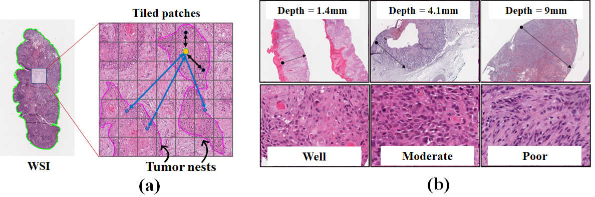
Figure 1: (a) Non-local semantic (blue) and local spatial (black) dependencies between tumor regions with the same grade. (b) Correlation between depth and grade: Worse-grade tumor invades deeper into the skin tissue reaching higher depth from the skin surface.

cSCC tumor grading presents three main challenges: (i) grade difference of tumor regions within the same WSI, (ii) the need for contextual information for determining tumor grade, and (iii) limited data. (i) A given cSCC WSI might comprise multiple tumor regions with varying grades. Pathologists implicitly rank the tumor regions based on their cellular differentiation (from well to poor), providing the grade of the most severe tumor region as the overall label (NCI 2023). Thus, the model must determine the implicit grade order to identify the most severe tumor region and de-emphasize the importance of irrelevant tumor regions, even if the less severe tumor captures a larger portion of the WSI. (ii) cSCC grading is context-aware because pathologists consider the local tumor neighborhood (tumor microenvironment) as well as long-range relations between distant tumor regions to determine the WSI-level grade label. On the one hand, existing studies (Chen et al. 2021) employ spatial proximity-based graphs to capture information from the tumor microenvironment, but they often overlook long-range semantic dependencies between tumor regions with similar morphology. On the other hand, although graph transformer-based methods (Zheng et al. 2022) incorporate all pairwise patch relationships, they are prone to overfitting on limited-size WSI datasets. Thus, there is a need for approaches that balance the information from local and long-range relations between patches. (iii) Limited number of WSIs and an imbalance in the number of low-risk (well-differentiated) vs. high-risk (moderately and poorly-differentiated) cases further exacerbate the previous two challenges.

To overcome these challenges, we propose an approach that utilizes rank-aware contextual reasoning (RACR) to leverage contextual information and maintain the ordinal ranking of tumor grades. Our model, RACR-MIL, predicts WSI tumor grade via four main steps. First, we divide the tissue into patches and extract local patch features using a self-supervised pre-trained encoder, in line with existing methods (Li, Li, and Eliceiri 2021). Second, we define a graph on the tissue patches that captures both local (spatial) and non-local (semantic) dependencies between the patches. We derive multiscale features using self-attention-based graph convolution to incorporate contextual information. Third, we utilize attention-based patch feature aggregation (Ilse, Tomczak, and Welling 2018) to derive a WSI-level feature for grade classification. We augment the attention computation with a rank ordering mechanism that assigns higher weights to higher-grade tumor regions. Finally, we incorporate tumor depth as an auxiliary prediction task for regularizing attention to relevant tumor patches.

Our work presents three key innovations. First, to emulate the ordinal grading protocol implicitly followed by pathologists, we introduce a two-part rank-ordering loss to train the attention network. It consists of (i) an interclass constraint, which compares patches from different grades and imposes higher attention on more severe tumor patches, and (ii) an intraclass constraint, which imposes higher attention on more likely patches within the same grade. We obtain the grade of each patch by pseudo-labeling the patches based on their grade class-likelihoods. Rank ordering enables our model to consistently assign higher importance to the most severe tumor region(s), improving tumor localization.

Second, we demonstrate the effectiveness of combining local and non-local dependencies between tissue regions for grading. We construct a WSI graph with patches as nodes and edges defined using a combination of spatial proximity and semantic similarity, i.e., patch feature similarity. This enables long-range message passing extending beyond the immediate neighbors in WSI during graph convolution, allowing us to capture broader tumor structure. Incorporating spatial and semantic context improves the localization and classification of higher-risk tumors (moderately and poorly differentiated), which existing methods find difficult to classify correctly.

Finally, we introduce the use of tumor depth as an auxiliary training signal to enhance grade classification. Prior studies have shown that tumor grade is significantly associated with tumor depth (Derwinger et al. 2010; Cruz et al. 2007; Kudo et al. 2022). Well-differentiated cSCC tumors have lower depth, while poorly-differentiated tumors invade deeper into the tissue (Derwinger et al. 2010). To capture the relationship between depth and grade, we develop a multitask framework that predicts depth and grade jointly, sharing the patch features between them.

We evaluated our approach on a real-world cSCC dataset of 718 WSIs. RACR-MIL achieves an F1-score of 0.796 and a 19.6% improvement in classifying challenging moderate-grade tumors compared to existing MIL methods. Qualitative analysis of the attention distribution revealed that the tumor region(s) localized by the model aligns well with fine-grained tumor annotations by pathologists, and the attention distribution is consistent over tumor region(s) of interest. Ablation analyses showed that each proposed innovation contributes to improving certain aspects of model performance. Our key contributions are as follows:

1. We propose the first weakly supervised framework for multi-class cSCC grading in pathology images.

2. Our model captures spatial and semantic dependency within a WSI using a graph network, enabling us to capture higher-order relationships between tumor patches. To our knowledge, we are the first to leverage semantic edges for WSI grading.

3. We introduce an ordinal ranking constraint on the attention of the patches that mimics pathologists’ implicit tumor grade ordering.

4. We exploit the additional training signal from tumor depth, a related cSCC tumor prognostic factor, using multitask learning.

5. Our innovations lead to state-of-the-art grade classification performance which is resilient to class imbalance and results in greater alignment with fine-grained tumor annotations compared to existing methods.

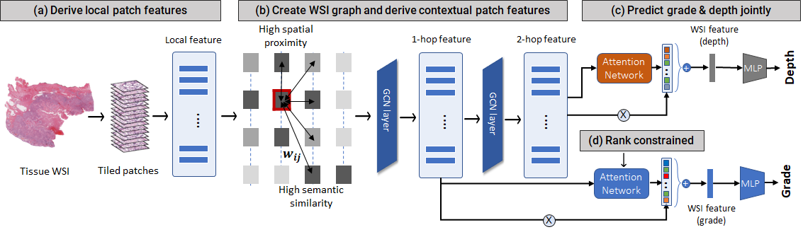
Figure 2: The proposed model. (a) Tissue tiling and local feature extraction. (b) Derivation of contextual patch features using self-attention-based graph convolution, taking spatial and semantic dependency into account. (c) Joint prediction of grade and depth using multiscale contextual features. (d) Rank-order constraint on the attention network.

Methodology

Each WSI is represented as a bag $b$ of patches $X_{b}=\{x_{n}\}_{n=1}^{N}$. $N$ denotes the number of non-overlapping patches in a WSI, and $b\in\{1,2...B\}$, where $B$ is the number of training samples. The patch-level labels $y_{n}$ are unknown, and we have access only to the bag label $Y_{b}\in$ {normal, well, moderate, poor}.

Tissue Feature Encoding

Tissue feature extraction consists of local feature extraction using self-supervised learning followed by contextual feature extraction using a graph convolution network (GCN).

Local feature extraction

We leverage self-supervised learning (SSL) to pre-train the patch feature extractor using unlabeled patches extracted from WSIs. To capture fine-grained pathological features (e.g., nuclei details, cell distribution, tumor microenvironment), we extract $448\times 448$ sized non-overlapping patches at $20X$ magnification. We use Nest-S (Zhang et al. 2022), a hierarchical transformer, to extract patch features. We pre-train the feature extractor using DINO (knowledge distillation-based SSL) (Caron et al. 2021) because of its promising performance in MIL-based classification tasks (Chen et al. 2022). After pre-training, the transformer network is used as an offline feature extractor to derive $d$-dimensional feature $f_{n}\in\mathcal{R}^{d}$ for each patch $x_{n}$, leading to a WSI representation of $\{f_{n}\}_{n=1}^{N}$.

Since the pre-trained features $f_{n}$ are agnostic to the downstream task, we project them into a lower-dimensional space using a multi-layer perceptron (MLP) with nonlinear activation to get local patch features $h_{n}^{0}$. We train the MLP along with the graph convolution network and the rank-aware grade classifier. Thus, the resulting local patch feature $h_{n}^{0}$ potentially captures information specific to grade and de-emphasizes information irrelevant to the downstream task.

Contextual feature extraction

Graph Definition: To extract contextual information capturing spatial and semantic dependency, we derive an undirected graph from each WSI $G=(V,A)$ with patches as nodes $V$ and adjacency matrix $A\in\mathcal{R}^{N\times N}$, which represents the connections between the nodes. The edges capture the pathology-related structure and interdependence among tumor regions via two types of contextual dependencies incorporated into the adjacency matrix $A$: (i) $A_{sem}$, which represents non-local dependencies between patches that may be spatially distant, but are similar in terms of their tissue structure (grade) in the feature space; and (ii) $A_{sp}$, which captures local dependencies between a tumor patch and its spatially neighboring patches in the tumor microenvironment. We only consider edges to the K-nearest neighbors in both the semantic and spatial space.

$A_{sem}$ is defined using pairwise feature similarity between patches:

$$A_{sem}(i,j)=\exp\bigg{(}\frac{-d^{sem}_{ij}}{0.1}\bigg{)};d^{sem}_{ij}=1-\frac{f_{i}\cdot f_{j}}{||f_{i}||_{2}||f_{j}||_{2}}$$ (1)

where $d_{ij}^{sem}$ represents the semantic distance between patches $i,j$ with features $f_{i}$ and $f_{j}$. $j\in[1,N]$ denotes the $K$-nearest neighbors of the $i^{th}$ patch ($K=4$). We pre-process the derived semantic graph $A_{sem}$ using personalized PageRank kernel-based graph diffusion (Gasteiger, Weißenberger, and Günnemann 2019). This amplifies long-range connections between tumor regions by generating additional edges beyond 1-hop neighbors in the feature space.

$A_{sp}$ is computed using inverse distance weighing across spatially K-nearest patches.

$$A_{sp}(i,j)=\exp\bigg{(}\frac{-d^{sp}_{ij}}{2}\bigg{)};d^{sp}_{ij}=\sqrt{(s_{i}-s_{j})^{2}+(t_{i}-t_{j})^{2}}$$ (2)

where $d_{ij}^{sp}$ represents the spatial distance between patches $i,j$ with spatial coordinates $(s_{i},t_{i})$ and $(s_{j},t_{j})$, respectively. We use $K=8$ to connect each patch to its immediate neighboring patches in the tissue.

The adjacency matrix $A$ is the average of the spatial and semantic components $\bigg{(}A=\frac{A_{sem}+A_{sp}}{2}\bigg{)}$.

Graph Feature Aggregation: We leverage graph convolution with residual mapping (Li et al. 2020) to derive multiscale contextual patch features $(h^{1}_{n},h^{2}_{n})$ from the local patch feature $h^{0}_{n}$ and adjacency matrix $A$. Each convolution layer uses message-passing to propagate feature information from the 1-hop connected nodes $j$ of a node $i$ ($A_{ij}>0$) and updates node features via the following operation:

$$H^{l+1}=H^{l}+GConv(H^{l},A;W^{l})$$ (3)

where $H^{l}=[h^{l}_{1},h^{l}_{2}...,h^{l}_{N}]$ and $W^{l}$ are the trainable parameters of layer $l$. We use two $GConv(\cdot)$ layers and consider two design choices for $GConv(\cdot)$.

1. Fixed edge weights: We use vanilla graph convolution network (GCN)(Kipf and Welling 2016) with weighted message passing using predefined edge weights from adjacency matrix $A$:

   $$GConv(\cdot)=ReLU(\tilde{D}^{-\frac{1}{2}}\tilde{A}\tilde{D}^{-\frac{1}{2}}H^{l}W^{l})$$ (4)

   where $\tilde{D}=\sum_{j}{\tilde{A}(i,j)}$ is the diagonal matrix of $\tilde{A}=A+I$. $\tilde{A}$ is used to avoid oversmoothing (Kipf and Welling 2016).

2. Dynamic edge weights: Alternatively, we can leverage graph attention-based convolution (Shi et al. 2020) to dynamically define edge weights. This allows us to dynamically aggregate information from patches connected to a patch based on their pairwise similarity. We use a single attention head with masking to aggregate the neighboring patch features:

   $$GConv(\cdot)=ReLU\bigg{[}softmax\bigg{(}\frac{Q^{l}K^{l}}{\sqrt{d}}+M\bigg{)}H^{l}W^{l}\bigg{]}$$ (5)

   where $Q^{l}=H^{l}W_{Q}^{l},K^{l}=H^{l}W_{K}^{l}$ and $M$ is the attention mask ($M_{ij}=0$ if $A_{ij}>0$, else $M_{ij}=-\infty$). $W^{l}_{Q},W^{l}_{K}$, $W^{l}$ are trainable parameters of layer $l$ and $W^{l}_{Q},W^{l}_{K}$ are used to learn the edge weights through the dot product $Q^{l}K^{l}$.

Multi-task training

Multi-task learning allows us to use additional information from auxiliary labels (depth) to aid main task prediction (grade). We selected depth as an auxiliary label because (i) it is easily available from diagnostic reports, (ii) it is derived from pathology images and reflects tissue structure surrounding the tumor, and (iii) it is well-correlated with grade (Dunn’s pairwise p-values are significant at a 10% level). We designed separate predictors for depth and grade while the graph network is shared between them to allow feature sharing and to ensure parameter efficiency.

Grade Classification

We use attention-based feature aggregation to determine the contribution of each patch to overall WSI prediction. Attention-based aggregation outperforms traditional pooling-based methods by up-weighing the most relevant patches. We leverage 1-hop contextual features to determine the normalized attention weight for each patch using a two-layer network:

$$w_{n}=\frac{\exp[a^{T}\tanh(U\cdot h^{1}_{n})]}{\sum_{i}\exp[a^{T}\tanh(U\cdot h^{1}_{n})]}$$ (6)

where $a\in\mathcal{R}^{d}$ and $U\in\mathcal{R}^{d\times d}$ are learnable parameters. The attention score is based on the formulation proposed by Ilse et al. (Ilse, Tomczak, and Welling 2018). The overall WSI representation is the attention-weighted average of normalized 1-hop patch features: $W^{diff}_{b}=\sum_{n=1}^{N}w_{n}\frac{h^{1}_{n}}{||h^{1}_{n}||}$.

The WSI class-likelihood is computed using a single-layer MLP cosine softmax classifier $\phi$:

$$p_{b,c}=\frac{\exp[-\mathcal{D}(\phi(W^{diff}),z_{c})]}{\sum_{c^{\prime}}\exp[-\mathcal{D}(\phi(W^{diff}),z_{c^{\prime}})]}$$ (7)

where $c\in\{0,1,2,3\}$ representing {normal, well, moderate, poor}, $\mathcal{D}$ represents cosine distance and $z_{c}$ is the prototype (class centroid) of grade class $c$ defined as $z_{c}=\frac{1}{N_{c}}\sum_{n:y_{n}=c}\phi(\frac{h_{n}^{1}}{||h_{n}^{1}||})$. To counter class imbalance due to a lower proportion of poorly differentiated cases, we leverage class-balanced sampling (Cui et al. 2019) during training. We use the ground-truth WSI grade label $Y_{b}$ to compute our MIL-based grade classification loss:

$$\mathcal{L}_{grade}=-\sum_{b=1}^{B}\sum_{c}\mathbf{1}(Y_{b}=c)\log(p_{b,c}),$$ (8)

Ordinal Ranking of Patches

We apply two ranking constraints on the attention network to ensure consistent ranking of tumor regions: (i) an interclass constraint to impose higher attention values for worse patches, and (ii) an intraclass constraint to impose higher attention values for more likely patches within the same class.

Interclass ranking: Pathologists determine the WSI grade based on the grade of the most severe tumor region by implicitly ranking the different tumor sections based on their severity. Motivated by this, we propose to enforce a ranking by using pairwise inequality constraints between patches, such that a more severe patch is ranked higher by the attention network ($w_{n}^{normal}<w_{n}^{well}<w_{n}^{moderate}<w_{n}^{poor})$.

To do so, we require the grade of each patch, which is unavailable. Therefore, we pseudo label the patches using a threshold on their class probabilities $p_{n,c}$:

$$p_{n,c}=p(y_{n}=c|h^{1}_{n})=\frac{\exp[-\mathcal{D}(\phi(h_{n}^{1}),z_{c})]}{\sum_{c^{\prime}}\exp[-\mathcal{D}(\phi(h_{n}^{1}),z_{c^{\prime}})]}$$ (9)

We set $y^{pseudo}_{n}$ = $c$ if $p_{n,c}$ $>$ $0.6$, $c$ is the grade class. We derive a set of pairs $(i,j)$ of pseudo-labeled patches belonging to two adjacent classes, $Z$ = $\{(i,j);y^{pseudo}_{i}=c,y^{pseudo}_{j}=c+1,\text{for some }c\in\{0,1,2\}\}$ and impose a soft ordinal constraint on their attention weights ($w_{i}<w_{j}$) using the pairwise ranking loss:

$$\mathcal{L}_{inter}=\sum_{i,j\in Z}\log[1+\exp(w_{i}-w_{j})]$$ (10)

Intraclass ranking: In addition, we impose intraclass ranking on the patches to ensure that the most confident patches (with higher $p_{n,c}$) within a particular grade class are weighted higher during feature aggregation. We focus on the patches with the highest attention weights or class probability, i.e., $\mathcal{S}=\{n;n\in TopK(w_{n})\cup TopK(p_{n,c})\}$ for $K=50$. Next, we derive a set of pairs $(i,j)$ using their class probabilities $\tilde{Z}$ = $\{(i,j);p_{i,c}<p_{j,c}-\delta,\text{for }i,j\in\mathcal{S},c\in\{0,1,2,3\}\}$, where $\delta=0.1$ is used to limit the number of pairs due to computational constraints. We impose a pairwise ranking loss on the attention network for patches in $\tilde{Z}$:

$$\mathcal{L}_{intra}=\sum_{i,j\in\tilde{Z}}\log[1+\exp{(w_{i}-w_{j})}]$$ (11)

For a pair of patches $(i,j)$, this loss enforces that if $p_{j,c}>p_{i,c}$, then attention weight $w_{j}>w_{i}$.

Depth Prediction

Depth values are continuous and depend on the global tissue structure. Since depth is continuous, we formulate depth prediction as a regression task. The depth predictor uses a single-layer MLP regressor $W_{reg}$ and a two-layer attention network. We use 2-hop patch features $h^{2}_{n}$ for both regression and attention networks since it captures more contextual information, which is useful for depth prediction.

The WSI-level feature for depth prediction is $H_{b}^{depth}=\sum_{n=1}^{N}w^{d}_{n}\cdot h^{2}_{n}$, where $w^{d}_{n}$ is the attention weight computed from $h^{2}_{n}$ by using an equation similar to equation 6.

The depth predictor is trained using the robust Geman-McClure loss (Barron 2019) to reduce sensitivity to large errors from outlier depth values ($>10mm$):

$$\mathcal{L}_{depth}=\frac{2(\hat{Y}_{b}^{depth}-Y_{b}^{depth})^{2}/c^{2}}{2(\hat{Y}_{b}^{depth}-Y_{b}^{depth})^{2}/c^{2}+4}$$ (12)

where $\hat{Y}_{b}^{depth}=W_{reg}\cdot(H^{depth}_{b})^{T}$ and $c=2$ is the scale parameter.

Overall Loss: The overall loss combines the grade classification loss, depth prediction loss, and the interclass and intraclass attention ranking losses. To balance the losses, we used the weighing factors $\lambda_{0}$, $\lambda_{1}$ and $\lambda_{2}$, which are determined using hyperparameter tuning:

$$\mathcal{L}_{total}=\mathcal{L}_{grade}+\lambda_{0}\mathcal{L}_{depth}+\lambda_{1}\mathcal{L}_{inter}+\lambda_{2}\mathcal{L}_{intra}\\$$ (13)

Experimental Setup

Datasets

We utilized a cSCC dataset from a leading US-based hospital consisting of 718 hematoxylin and eosin (H&E) stained WSIs scanned at $40X$ magnification for training and evaluation. The dataset was collected from 2017-2022 and reviewed by a group of 4 expert dermatopathologists. The dataset contains 150 normal, 383 well-differentiated, 108 moderately differentiated, and 77 poorly differentiated cases. A majority of patients were white.

Pre-processing

To remove background regions and irrelevant tissue sections, we pre-processed each WSI using thresholding and morphological operations (Lu et al. 2021). Each tissue region was downsampled to $20X$ magnification and tiled into non-overlapping $448\times 448$ patches. Patches with minimal texture were removed using image gradient-based entropy.

Training details

We performed stratified 5-fold cross-validation using a 64:16:20 split between training/validation/test sets. The GCN feature extractor and task-specific predictors were jointly trained using the Adam optimizer with a batch size of 16 and a learning rate of $1e^{-4}$ for 60 epochs. The evaluation metrics were: cross-validated average of classwise accuracy (ACC), macro-averaged F1 score, AUC score, and Matthews Correlation Coefficient (MCC).

Tumor localization

Fine-grained tumor annotations were obtained to determine the extent of overlap of tumors with the most-probable tumor regions as predicted by the model. 24 WSIs from the test set were randomly chosen and annotated by two senior pathologists. Each pathologist marked the grades of up to seven most relevant tumor regions in each WSI.

Baselines

We compared our model with state-of-the-art attention-based MIL models, including methods that treat patches independently (ABMIL (Ilse, Tomczak, and Welling 2018), Gated ABMIL (GABMIL) (Ilse, Tomczak, and Welling 2018), CLAM-MB (Lu et al. 2021)) and contextual-dependency-based methods (PatchGCN (Chen et al. 2021), DSMIL (Li, Li, and Eliceiri 2021), TransMIL (Shao et al. 2021)). We also compared variants of RACR-MIL that included only some of the proposed innovations (spatial vs semantic contextual features, fixed vs learned edge weights, attention ranking) to evaluate their contribution to overall performance. In order to ensure a fair comparison, we utilized the same pre-trained model as the feature extractor for all approaches. We adjust the hyperparameters of existing approaches (embedding size, dropout rate, learning rate) to achieve optimal performance on our dataset. We achieve best test accuracy using $\lambda_{0}=1.0$, $\lambda_{1}=0.5$ and $\lambda_{2}=0.25$.

Table 1: Comparison of the proposed model with state-of-the-art existing attention-based methods. Bold and underline indicate the highest and second highest performance. ’Mod’ represents moderate-differentiation.

Methods	F1	Precision	Recall	ACC (Well)	ACC (Mod)	ACC (Poor)	ACC (Normal)	AUC (High vs Low Risk)	MCC
Non-contextual Approaches
Max Pooling	0.730	0.758	0.718	0.943	0.385	0.675	0.868	0.652	0.706
Mean Pooling	0.739	0.740	0.745	0.872	0.508	0.713	0.887	0.918	0.696
CLAM-MB	0.761	0.769	0.760	0.890	0.583	0.675	0.893	0.945	0.722
GABMIL	0.778	0.793	0.775	0.922	0.530	0.740	0.907	0.951	0.749
ABMIL	0.774	0.778	0.779	0.901	0.556	0.739	0.920	0.956	0.745
Contextual Approaches
PatchGCN	0.791	0.793	0.795	0.914	0.596	0.792	0.901	0.939	0.762
DSMIL	0.794	0.785	0.772	0.920	0.596	0.779	0.920	0.950	0.764
TransMIL	0.710	0.726	0.719	0.893	0.352	0.739	0.893	0.884	0.676
RACR-MIL (Graph + Rank)	0.796	0.783	0.823	0.830	0.713	0.830	0.920	0.955	0.753
RACR-MIL (Graph + Depth + Rank)	0.775	0.776	0.786	0.893	0.562	0.775	0.913	0.949	0.746

Results

Grade Classification

RACR-MIL outperforms state-of-the-art attention models by achieving 2-9% improvement in F1-score over existing non-contextual methods (Max/Mean Pooling, CLAM-MB, GABMIL, ABMIL; Table 1). It achieves a higher classification accuracy for higher-risk tumors (Mod + Poor) compared to the self-attention-based contextual methods TransMIL and DSMIL. Our model outperforms TransMIL, which learns pairwise dependencies between all patches, by 12% because it explicitly incorporates spatial and semantic dependency while creating the graph. Moreover, compared to DSMIL and PatchGCN which incorporate semantic dependency and spatial dependency respectively, our approach achieves slightly higher F1-score and is less prone to overfitting on the dominant well-differentiated class. Our model achieves the best performance in classifying the most challenging class (moderately differentiated) with 19.6% higher accuracy compared to the next best method (DSMIL).

All three innovations in the framework contribute to improvement in grade classification. Graph network-based contextual features combined with rank-ordering loss achieves the highest improvement in F1-score. The higher accuracy is due to the improved feature space that enables better rank ordering and separation of patches that belong to different grade classes (see Appendix). Including depth as an auxiliary task leads to a reduction in F1-score. This might be because depth is a geometric concept, and using 2-hop contextual features might not capture all of the relevant structural information for predicting depth accurately. However, qualitative analysis of tumor localization shows that using depth allows the model to localize the tumor better, capturing more tumor patches corresponding to the grade label.

Table 2: Impact of ranking ordering constraint and multitask learning using depth as an auxiliary task. ‘RACR-MIL[Fixed] represents leveraging a graph with fixed edge weights, and RACR-MIL[Learnt] represents leveraging a graph with self-attention-based dynamic edge weights.

Methods	F1	Precision	Recall	ACC (Well)	ACC (Mod)	ACC (Poor)	ACC (Normal)	AUC (High vs Low Risk)	MCC
ABMIL	0.774	0.778	0.779	0.901	0.556	0.739	0.920	0.956	0.745
+ Rank	0.786	0.783	0.800	0.896	0.601	0.815	0.887	0.951	0.756
RACR-MIL [Fixed]	0.779	0.775	0.795	0.849	0.640	0.791	0.900	0.949	0.732
+ Rank	0.791	0.787	0.810	0.870	0.638	0.831	0.900	0.952	0.754
+ Depth	0.768	0.764	0.780	0.883	0.532	0.779	0.925	0.940	0.734
RACR-MIL [Learnt]	0.754	0.750	0.773	0.825	0.583	0.791	0.893	0.951	0.703
+ Rank	0.796	0.783	0.823	0.830	0.713	0.830	0.920	0.955	0.753
+ Depth	0.775	0.776	0.786	0.893	0.562	0.775	0.913	0.949	0.746

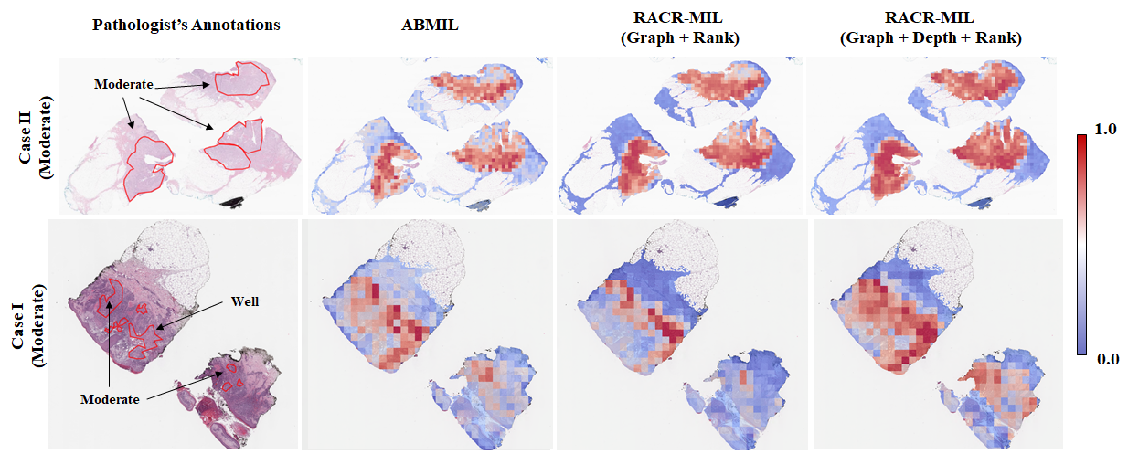
Figure 3: Normalized attention heatmaps highlighting the tumor ROI identified by different models. The patch level annotations for tumor grade are shown in red in the leftmost panels. In the heatmaps, red indicates high attention region and blue indicates a low attention regions.

Tumor Localization - Qualitative Analysis

We evaluated the impact of the proposed innovations on tumor localization by studying the normalized attention heatmaps of two representative WSIs (Figure 3). The heatmaps were derived by scaling the attention weight $w_{n}$ for each patch $x_{n}$ across a WSI ( $a_{n}=\frac{w_{n}-w_{n}^{min}}{w_{n}^{max}-w_{n}^{min}}$). Our model localizes the tumor accurately, achieving high consistency with ground-truth fine-grained tumor annotations. Leveraging depth with graph and raking captures a larger portion of the tumor (cases I and II) while leveraging graph leads to fewer false positives (case II) compared to the baseline approach ABMIL.

Ablation Study

Semantic Dependency

We find that leveraging both spatial and semantic dependency leads to higher classification accuracy (Table 3). Using spatial dependency allows the model to give consistent importance to nearby tumor regions, and using semantic dependency allows it to aggregate and focus on the relevant spatially distant tumor regions with similar morphology.

Table 3: Impact of WSI graph (spatial edges only vs both spatial and semantic edges) on grade classification accuracy.

Method	F1	ACC (Well)	ACC (Mod)	ACC (Poor)	ACC (Normal)
Fixed Edge Weights (Spatial)	0.780	0.898	0.647	0.700	0.887
Fixed Edge Weights (Both)	0.791	0.870	0.638	0.831	0.900
Learnt Edge Weights (Spatial)	0.787	0.843	0.694	0.789	0.920
Learnt Edge Weights (Both)	0.796	0.830	0.713	0.830	0.920

Depth as Auxiliary Task

We find that the graph-based contextual features and depth information are complementary and incorporating depth further guides the attention weights toward key tumor sections leading to lesser false positives (Figure 3).

Rank Constraint

Using the rank-ordering constraint allows us to suitably weigh the tumor regions by focusing higher attention on the higher-grade tumor within a WSI (Figure 3). The rank-ordering constraint is widely applicable - applying it to the baseline ABMIL framework leads to improved F1-score with higher accuracy in classifying high-risk tumors. Furthermore, imposing this constraint improves the F1-score by 2% for ABMIL and upto 5% for our framework. Additionally, it improves classification accuracy across all grade classes in our framework. We speculate that the rank constraint assigns a higher score to worse-grade tumor regions during feature aggregation and allows for aligning the prediction probability with the WSI-level label assigned by the pathologist.

Fixed vs Learnt Edge Weights

Learning edge weights using graph attention is more effective than using predefined edge weights for higher-risk cases (Table 2). It is possible that dynamically learned edge resulted in better performance because the edge weights better reflected the similarities between task-relevant patches.

Related Work

A majority of weakly-supervised tumor grading studies focus on prostate cancer or breast cancer, with a few studies on skin cancer grading primarily focusing on melanoma. These studies have explored attention-based MIL and graph-based contextual features. We build upon and extend existing methods to address cSCC-specific challenges.

Attention-based MIL: Attention-based multiple instance learning (ABMIL) ((Ilse, Tomczak, and Welling 2018)) was the first attention-based approach that aggregated patch information using vanilla attention and a gating mechanism for tissues with limited tumor proportion. Later methods built on MIL by improving the patch feature representation. CLAM ((Lu et al. 2021)) extended ABMIL by introducing an additional hinge loss that discriminated between high and low-attention patches to improve the patch representation. The authors also proposed a multiclass version named CLAM-MB with class-specific attention weights. DSMIL ((Li, Li, and Eliceiri 2021)) and TransMIL ((Shao et al. 2021)) employed self-attention to learn global dependencies within the tissue. Recently, self-supervision techniques based on contrastive learning (Caron et al. 2021) have been employed to pre-train and enhance feature extractors during training. Previous studies have not explored the use of auxiliary task labels (such as depth) or rank ordering of tumor regions.

Graph-based methods: Studies using graph networks with attention primarily focus on incorporating the spatial dependency between neighboring patches (PatchGCN (Chen et al. 2021)) and learning multiscale relationships using self-attention (Graph Transformer (Zheng et al. 2022)). Graph transformer-based approaches encode all pairwise dependencies for learning global relationships resulting in increased complexity and a possibility of overfitting on limited datasets. GCN-MIL (Xiang et al. 2023) proposed a graph convolution network for prostate cancer grading by defining a graph using sampled patches and edges based on spatial proximity. Existing methods have not leveraged long-distance semantic relationships for creating the graph.

Conclusion

We developed RACR-MIL, a novel approach for cSCC WSI tumor grading that incorporated spatial and semantic graph-based contextual features, auxiliary task information (tumor depth), and rank-ordering of tumor regions. The model achieved improved tumor grading on a real-world dataset compared to existing methods and also led to improved tumor localization. The proposed innovations are generic and applicable to existing WSI tumor grading methods, as shown in the ablation study. Our approach has the potential to enhance manual tumor grading as an AI assistant.

There are several limitations of this study, that we will address in future work. (i) The model can confuse non-tumor patches with tumor patches, resulting in false positives. Improved feature and contextual information extraction might help in separating different cell types in the feature space. (ii) Including depth as an auxiliary task did not improve grading. Depth is a geometric concept that requires identifying the tissue surface (epidermis). Expressing the global structure relevant to depth prediction may help. (iii) Clinical translation of the proposed method requires quantification of the uncertainty associated with the prediction to build trust. (iv) Finally, the clinical utility of the proposed approach in reducing inter-pathologist variability needs to be evaluated.

References

- Barron (2019) Barron, J. T. 2019. A general and adaptive robust loss function. In Proceedings of the IEEE/CVF Conference on Computer Vision and Pattern Recognition, 4331–4339.
- Caron et al. (2021) Caron, M.; Touvron, H.; Misra, I.; Jégou, H.; Mairal, J.; Bojanowski, P.; and Joulin, A. 2021. Emerging properties in self-supervised vision transformers. In Proceedings of the IEEE/CVF international conference on computer vision, 9650–9660.
- Chen et al. (2022) Chen, R. J.; Chen, C.; Li, Y.; Chen, T. Y.; Trister, A. D.; Krishnan, R. G.; and Mahmood, F. 2022. Scaling vision transformers to gigapixel images via hierarchical self-supervised learning. In Proceedings of the IEEE/CVF Conference on Computer Vision and Pattern Recognition, 16144–16155.
- Chen et al. (2021) Chen, R. J.; Lu, M. Y.; Shaban, M.; Chen, C.; Chen, T. Y.; Williamson, D. F.; and Mahmood, F. 2021. Whole Slide Images are 2D Point Clouds: Context-Aware Survival Prediction Using Patch-Based Graph Convolutional Networks. In International Conference on Medical Image Computing and Computer-Assisted Intervention, 339–349. Springer.
- Cruz et al. (2007) Cruz, J. J.; Ocaña, A.; Del Barco, E.; and Pandiella, A. 2007. Targeting receptor tyrosine kinases and their signal transduction routes in head and neck cancer. Annals of oncology, 18(3): 421–430.
- Cui et al. (2019) Cui, Y.; Jia, M.; Lin, T.-Y.; Song, Y.; and Belongie, S. 2019. Class-balanced loss based on effective number of samples. In Proceedings of the IEEE/CVF conference on computer vision and pattern recognition, 9268–9277.
- Derwinger et al. (2010) Derwinger, K.; Kodeda, K.; Bexe-Lindskog, E.; and Taflin, H. 2010. Tumour differentiation grade is associated with TNM staging and the risk of node metastasis in colorectal cancer. Acta Oncologica, 49(1): 57–62.
- Gasteiger, Weißenberger, and Günnemann (2019) Gasteiger, J.; Weißenberger, S.; and Günnemann, S. 2019. Diffusion improves graph learning. Advances in neural information processing systems, 32.
- Ilse, Tomczak, and Welling (2018) Ilse, M.; Tomczak, J.; and Welling, M. 2018. Attention-based deep multiple instance learning. In International conference on machine learning, 2127–2136. PMLR.
- Kipf and Welling (2016) Kipf, T. N.; and Welling, M. 2016. Semi-supervised classification with graph convolutional networks. arXiv preprint arXiv:1609.02907.
- Kudo et al. (2022) Kudo, M. S.; Gomes de Souza, V. M.; Estivallet, C. L. N.; de Amorim, H. A.; Kim, F. J.; Leite, K. R. M.; and Moraes, M. C. 2022. The value of artificial intelligence for detection and grading of prostate cancer in human prostatectomy specimens: A validation study. Patient Safety in Surgery, 16(1): 1–9.
- Li, Li, and Eliceiri (2021) Li, B.; Li, Y.; and Eliceiri, K. W. 2021. Dual-stream multiple instance learning network for whole slide image classification with self-supervised contrastive learning. In Proceedings of the IEEE/CVF conference on computer vision and pattern recognition, 14318–14328.
- Li et al. (2020) Li, G.; Xiong, C.; Thabet, A.; and Ghanem, B. 2020. Deepergcn: All you need to train deeper gcns. arXiv preprint arXiv:2006.07739.
- Lu et al. (2021) Lu, M. Y.; Williamson, D. F.; Chen, T. Y.; Chen, R. J.; Barbieri, M.; and Mahmood, F. 2021. Data-efficient and weakly supervised computational pathology on whole-slide images. Nature biomedical engineering, 5(6): 555–570.
- Mun et al. (2021) Mun, Y.; Paik, I.; Shin, S.-J.; Kwak, T.-Y.; and Chang, H. 2021. Yet another automated Gleason grading system (YAAGGS) by weakly supervised deep learning. npj Digital Medicine, 4(1): 99.
- NCI (2023) NCI. 2023. Code for Histologic Grading and Differentiation | SEER Training. Accessed 2023-04-07.
- Otálora et al. (2021) Otálora, S.; Marini, N.; Müller, H.; and Atzori, M. 2021. Combining weakly and strongly supervised learning improves strong supervision in Gleason pattern classification. BMC Medical Imaging, 21(1): 1–14.
- Severson et al. (2020) Severson, K.; Ederaine, S.; Montoya, J.; Butterfield, R.; Zhang, N.; Besch-Stokes, J.; Hughes, A.; Ochoa, S.; Nelson, S.; DiCaudo, D.; et al. 2020. 462 Examination of current staging systems in cutaneous squamous cell carcinoma. Journal of Investigative Dermatology, 140(7): S61.
- Shao et al. (2021) Shao, Z.; Bian, H.; Chen, Y.; Wang, Y.; Zhang, J.; Ji, X.; et al. 2021. Transmil: Transformer based correlated multiple instance learning for whole slide image classification. Advances in neural information processing systems, 34: 2136–2147.
- Shi et al. (2020) Shi, Y.; Huang, Z.; Feng, S.; Zhong, H.; Wang, W.; and Sun, Y. 2020. Masked label prediction: Unified message passing model for semi-supervised classification. arXiv preprint arXiv:2009.03509.
- Silva-Rodriguez et al. (2021) Silva-Rodriguez, J.; Colomer, A.; Dolz, J.; and Naranjo, V. 2021. Self-learning for weakly supervised gleason grading of local patterns. IEEE journal of biomedical and health informatics, 25(8): 3094–3104.
- Thompson et al. (2016) Thompson, A.; Kelley, B.; Prokop, L.; et al. 2016. Risk factors for cutaneous squamous cell carcinoma recurrence, metastasis, and disease-specific death: A systematic review and meta-analysis. JAMA Dermatology, 52(4): 419–428.
- Tokez et al. (2020) Tokez, S.; Hollestein, L.; Louwman, M.; Nijsten, T.; and Wakkee, M. 2020. Incidence of multiple vs first cutaneous squamous cell carcinoma on a nationwide scale and estimation of future incidences of cutaneous squamous cell carcinoma. JAMA dermatology, 156(12): 1300–1306.
- Xiang et al. (2023) Xiang, J.; Wang, X.; Wang, X.; Zhang, J.; Yang, S.; Yang, W.; Han, X.; and Liu, Y. 2023. Automatic diagnosis and grading of Prostate Cancer with weakly supervised learning on whole slide images. Computers in Biology and Medicine, 152: 106340.
- Zhang et al. (2022) Zhang, Z.; Zhang, H.; Zhao, L.; Chen, T.; Arik, S. Ö.; and Pfister, T. 2022. Nested hierarchical transformer: Towards accurate, data-efficient and interpretable visual understanding. In Proceedings of the AAAI Conference on Artificial Intelligence, volume 36, 3417–3425.
- Zheng et al. (2022) Zheng, Y.; Gindra, R. H.; Green, E. J.; Burks, E. J.; Betke, M.; Beane, J. E.; and Kolachalama, V. B. 2022. A graph-transformer for whole slide image classification. IEEE transactions on medical imaging, 41(11): 3003–3015.