Abstract

Variational flows allow practitioners to learn complex continuous distributions, but approximating discrete distributions remains a challenge. Current methodologies typically embed the discrete target in a continuous space—usually via continuous relaxation or dequantization—and then apply a continuous flow. These approaches involve a surrogate target that may not capture the original discrete target, might have biased or unstable gradients, and can create a difficult optimization problem. In this work, we develop a variational flow family for discrete distributions without any continuous embedding. First, we develop a measure-preserving and discrete (MAD) invertible map that leaves the discrete target invariant, and then create a mixed variational flow (MAD Mix) based on that map. Our family provides access to i.i.d. sampling and density evaluation with virtually no tuning effort. We also develop an extension to MAD Mix that handles joint discrete and continuous models. Our experiments suggest that MAD Mix produces more reliable approximations than continuous-embedding flows while being significantly faster to train.

1 Introduction

The Bayesian statistical framework allows practitioners to model complex relationships between variables of interest and to incorporate expert knowledge as part of inference in a principled way. This has become crucial with the advent of heterogeneous data, which is typically modeled using a mix of continuous and discrete latent variables. One popular methodology for inference in Bayesian models is variational inference (VI) (Jordan et al., 1999; Wainwright and Jordan, 2008), which involves finding a distribution in a variational family of candidate distributions that minimizes a divergence to the posterior. Distributions in the variational family usually enable both i.i.d. draws and tractable density evaluation, which allows practitioners to assess the quality of (and therefore optimize) the approximate distribution by estimating, e.g., the evidence lower bound (ELBO) (Blei et al., 2017).

State-of-the-art variational methods have been very successful in approximating continuous distributions. Of particular interest to this work are normalizing flows (Tabak and Turner, 2013; Dinh et al., 2015; Rezende and Mohamed, 2015; Kobyzev et al., 2020; Papamakarios et al., 2021), which leverage repeated applications of flexible bijective transformations to construct highly expressive approximations. Under mild conditions, some normalizing flows are universal approximators of continuous distributions when the number of repeated applications of the transformation (i.e., the depth of the flow) grows to infinity (Huang et al., 2018, 2020; Kong and Chaudhuri, 2020; Zhang et al., 2020; Lee et al., 2021). In recent work, Xu et al. (2023) designed flow-based variational families that have compute/accuracy trade-off theoretical guarantees, and which circumvent the need to optimize the parameters of the flow.

In contrast with the continuous setting, work on normalizing flows for approximating discrete distributions has been more limited. Bijections between discrete sets—i.e., permutations—can only rearrange the probability masses among the discrete values without changing their values (Papamakarios et al., 2021). Recent work has addressed this issue by embedding the discrete target distribution in a continuous space in various ways, and then approximating it with continuous flows.

One way to do this is to approximate the discrete distribution of interest with a continuous relaxation (Maddison et al., 2017; Jang et al., 2017; Tran et al., 2019; Hoogeboom et al., 2021b). In this case, one constructs a surrogate continuous distribution in the simplex parametrized by a temperature—at zero temperature, the approximation becomes the original discrete target. But relaxing a discrete distribution to a continuous one introduces a trade-off between the fidelity of the approximation and the difficulty of learning the flow: a low temperature distribution will be very “peaky” near the vertices of the simplex, causing gradient instability. Another continuous-embedding strategy is dequantization (Uria et al., 2013; Theis et al., 2016; Hoogeboom et al., 2021a; Nielsen et al., 2020; Zhang et al., 2021; Chen et al., 2022), whereby one adds continuous noise to the atoms of the discrete distribution. However, dequantization-based methodologies are incompatible with categorical data, since switching the labels results in a different dequantization. Previous work has also considered transformations that update discrete states by thresholding a continuous neural network (Hoogeboom et al., 2019; van den Berg et al., 2021; Tomczak, 2021), but this can bias the gradient estimates of the continuous flow. Yet another option is to encode a discrete distribution into a continuous distribution and optimize the encoder (Ziegler and Rush, 2019; Lippe and Gavves, 2021). But approximating a surrogate target density that takes values in an inherently different space introduces error even if the optimal approximation is eventually found.

In this work, we develop a flow-based variational family to approximate discrete distributions without embedding them into a continuous space. Our family is based on a new Measure-preserving And Discrete (MAD) map that leaves the discrete target invariant. The key idea behind MAD is to augment the discrete target with uniform variables, which we use to update each discrete variable via an inverse-CDF-like deterministic move. We then use the MAD map as a building block in a mixed variational flow (MixFlow) (Xu et al., 2023), which averages over repeated applications of MAD. We call the resulting variational family MAD Mix. Unlike the MixFlow instantiation in Xu et al. (2023), which assumes that the target distribution is continuous, our family is specifically designed to learn discrete distributions—both ordinal and categorical. We also show how to combine MAD with the discretized Hamiltonian dynamics from Xu et al. (2023) to approximate joint continuous and discrete targets, e.g., mixture models. Through multiple experiments, we compare MAD Mix with continuous-embedding normalizing flows, mean-field VI (Wainwright and Jordan, 2008), and Gibbs sampling. Our results show comparable sampling quality to Gibbs sampling, but with the ability to evaluate the density of the approximation—and therefore to assess its quality via the ELBO—as well as better training efficiency, stability, and approximation quality than both dequantized and relaxed normalizing flows.

2 Background

Consider a target distribution $\pi$ on a set $\mathcal{X}$. We assume that $x\in\mathcal{X}$ can contain both discrete- and real-valued elements, and that $\pi$ admits a density with respect to a product of Lebesgue and counting measures on their respective real-valued and discrete components. We will use the same symbol to denote both a distribution and its density. In the setting of Bayesian inference, $\pi$ is a posterior distribution whose density we can only evaluate up to a normalizing constant, $\pi(x)=p(x)/Z$, where $p$ is known but $Z=\int p$ is not.

In its most common form, variational inference (VI) refers to approximating $\pi$ with an element $q^{\star}$ of a family of parametric variational approximations $\mathcal{Q}=\{q_{\lambda}\mid\lambda\in\Lambda\}$. Usually, $q^{\star}=q_{\lambda^{\star}}$ is chosen to minimize the Kullback–Leibler divergence (Kullback and Leibler, 1951) between elements in $\mathcal{Q}$ and $\pi$:

$$\lambda^{\star} =\operatornamewithlimits{arg\,min}_{\lambda\in\Lambda}\mathrm{D_{KL}}\mathchoice{\left({{{{q_{\lambda}||\pi}}}}\right)}{({{{{q_{\lambda}||\pi}}}})}{({{{{q_{\lambda}||\pi}}}})}{({{{{q_{\lambda}||\pi}}}})}$$ (2)

$$=\operatornamewithlimits{arg\,min}_{\lambda\in\Lambda}\int_{\mathcal{X}}q_{\lambda}(x)\log\frac{q_{\lambda}(x)}{p(x)}\,\mathrm{d}x.$$ (3)

The normalizing constant $Z$ can be factored out of the KL divergence, which results in the optimization problem in Eq. 2 (Blei et al., 2017). Typically, $\mathcal{Q}$ is designed to allow both density evaluation and i.i.d. sampling from its elements. This enables the use of stochastic gradient optimization algorithms to find a stationary point of Eq. 2 (e.g., Ranganath et al., 2014; Kucukelbir et al., 2017).

Normalizing flows (Tabak and Turner, 2013; Rezende and Mohamed, 2015; Dinh et al., 2015; Kobyzev et al., 2020; Papamakarios et al., 2021) are a common approach to design such a $\mathcal{Q}$. Normalizing flows build an approximation $q_{\lambda}$ by applying a differentiable bijective map $T_{\lambda}$ that also has a differentiable inverse (i.e., a diffeomorphism) to a reference distribution $q_{0}$ on $\mathcal{X}$: $q_{\lambda}=T_{\lambda}q_{0}$. Here, $T_{\lambda}q_{0}$ is the pushforward of $q_{0}$ under $T_{\lambda}$. In practice, $T_{\lambda}$ is built by composing multiple “simple” maps $T_{\lambda}=T_{N,\lambda_{N}}\circ\cdots\circ T_{1,\lambda_{1}}$, each with their own parameters $\lambda_{n}$. If each $T_{n,\lambda_{n}}$ is invertible and differentiable then so is the resulting $T_{\lambda}$. Recent work has focused on designing maps $T_{n,\lambda_{n}}$ that satisfy two desiderata: the simple maps are easy to evaluate, invert, and differentiate, and the resulting family is highly expressive (e.g., it is a universal approximator as in Huang et al. (2018, 2020); Kong and Chaudhuri (2020); Zhang et al. (2020); Lee et al. (2021)). If $x$ is real-valued, the density of $q_{\lambda}$ can be written down using the determinant Jacobian of $T_{\lambda}$, $J_{\lambda}(x):=\left|\nabla_{x}T_{\lambda}(x)\right|$. Specifically, using the change-of-variables formula,

$$q_{\lambda}(x)=\frac{q_{0}(T_{\lambda}^{-1}(x))}{J_{\lambda}(T_{\lambda}^{-1}(x))},\qquad x\in\mathcal{X}.$$ (4)

If $x$ is discrete, the change-of-variables formula does not contain a determinant Jacobian term and so Eq. 4 becomes $q_{\lambda}(x)=q_{0}(T_{\lambda}^{-1}(x))$. However, bijections on discrete spaces are just permutations, and so it is impossible to build expressive approximations in this setting.

Beyond issues with discrete variables, normalizing flows require practitioners to optimize the flow parameters $\lambda$ as in Eq. 2, which can introduce additional optimization-related problems. Recent work addresses this issue by constructing flows with diffeomorphisms that are also ergodic and measure-preserving for $\pi$ (Xu et al., 2023). A map $T_{\lambda}$ is ergodic for $\pi$ if, when applied repeatedly, it does not get “stuck” in any non-trivial regions of $\mathcal{X}$, i.e., if $T_{\lambda}(A)=A$ implies $\pi(A)$ is either 0 or 1 for any measurable $A\subseteq\mathcal{X}$. $T_{\lambda}$ is measure-preserving for $\pi$ if it leaves the distribution of samples from $\pi$ invariant, that is, if $X\sim\pi$ implies $T_{\lambda}(X)\sim\pi$. A mixed variational flow (Xu et al., 2023), or MixFlow, is a mixture of repeated applications of such a $T_{\lambda}$. Regardless of whether $x$ is real- or discrete-valued, MixFlows have MCMC-like convergence guarantees in that they converge to the target in total variation for any value of $\lambda$ (Xu et al., 2023, Theorems 4.1–4.2):

$$q_{N,\lambda}:=\frac{1}{N}\sum_{n=0}^{N-1}T_{\lambda}^{n}q_{0},$$ (5)

$$\lim_{N\to\infty}\mathrm{D_{TV}}\mathchoice{\left({{{{q_{N,\lambda},\pi}}}}\right)}{({{{{q_{N,\lambda},\pi}}}})}{({{{{q_{N,\lambda},\pi}}}})}{({{{{q_{N,\lambda},\pi}}}})}=0,\quad\forall\lambda\in\Lambda.$$ (6)

The density $q_{N,\lambda}$ for real-valued $x\in\mathcal{X}$ can be evaluated by backpropagating the flow:

$$q_{N,\lambda}(x)=\frac{1}{N}\sum_{n=0}^{N-1}\frac{q_{0}(T_{\lambda}^{-n}(x))}{\prod_{j=1}^{n}J_{\lambda}(T_{\lambda}^{-j}(x))},$$ (7)

with $J_{\lambda}(x)=\left|\nabla_{x}T_{\lambda}(x)\right|$. Furthermore, i.i.d. samples can be generated by repeatedly pushing samples from $q_{0}$ through $T_{\lambda}$:

$$n\sim{\sf{Unif}}\{0,\dots,N-1\},\quad X_{0}\sim q_{0},\quad T_{\lambda}^{n}(X_{0})\sim q_{N,\lambda}.$$ (8)

Although the theoretical guarantees for MixFlows hold for continuous and discrete $x$, the instantiation provided by Xu et al. (2023) only applies to real-valued variables since it is based on Hamiltonian dynamics. Furthermore, as with normalizing flows, the density formula in Eq. 7 is only valid for continuous $x$. In the next section, we develop a measure-preserving map for discrete distributions and then show how to construct a MixFlow based on it, including extending the density formula from Eq. 7 to that setting.

3 Measure-preserving And Discrete MixFlows (MAD Mix)

In this section, we develop a novel measure-preserving bijection for discrete variables that does not embed the underlying distribution in a continuous space and that can be used in flow-based VI methodologies. We call this map MAD since it is Measure-preserving And Discrete. The key idea behind MAD is to augment the target density with a set of auxiliary uniform variables, which we then use to update the discrete components. Fig. 1 shows a single pass of the MAD map and Algorithm 1 contains pseudocode to evaluate it. We then construct a MixFlow based on the MAD map (MAD Mix) and discuss how to extend MAD Mix to work with joint discrete and continuous variables by combining it with the prior work on MixFlows in Xu et al. (2023).

3.1 Measure-preserving and discrete map

To build intuition, we first consider a simplified example where we approximate a univariate discrete target $\pi$. Without loss of generality, we assume $\mathcal{X}=\mathbb{N}$. In Section 3.2, we discuss how to use this simplification as a stepping stone for the case where $\pi$ is multivariate. We start by considering an augmented target density that contains a uniform variable $u\in[0,1]$:

$$\tilde{\pi}(x,u)=\pi(x)\mathds{1}_{[0,1]}(u).$$ (9)

We use $u$ to sequentially update the value of $x$ with an inverse CDF deterministic update. Specifically, we construct our map $T_{\mathrm{MAD}}$ by composing three steps:

Figure 1: One application of the MAD map to the initial values $(x_{0},u_{0})=(2,0.75)$ with target probabilities $\pi={\sf{Categorical}}(0.1,0.4,0.4,0.1)$. Each plot contains the CDF of $\pi$. In the first plot, $u_{0}$ represents the proportion of mass between $x_{0}=2$ and $1$. In the second plot, $u_{0}$ is transformed into $\rho$—which indicates where in the CDF of $\pi$ the initial value $x_{0}$ lies at. Then, in the third plot, $\rho$ is shifted vertically by $\xi=0.45$ to $\tilde{\rho}$, which produces a new value $x_{1}$ via the inverse CDF trick. Finally, $\tilde{\rho}$ gets transformed into $u_{1}$, which represents the proportion of mass between $x_{1}=3$ and $2$.

(1) Mapping uniform to $\rho$-space

Let $F$ denote the CDF of $\pi$ and define $F(0)=0$. Then we transform the uniform variable $u$ into $\rho$:

$$\rho=F(x-1)+u\pi(x).$$ (10)

While $u$ and $x$ are independent a priori, this update introduces a dependence relationship between them by allowing the uniform variable to switch between two interpretations: $\rho\in[0,1]$ is the usual uniform $[0,1]$ variable in the inverse CDF method for drawing $x$, while $u$ can be thought of as a proportion of the mass at $x$ and is independent of the value of $x$. The first two panels of Fig. 1 show an example where $x=2$, $\pi(2)=0.4$, and $u=0.75$. Here, $u$ indicates that $\rho$ lies 75% of the way between $x=1$ and $x=2$, and hence $\rho=F(1)+0.75\pi(2)=0.1+0.75\times 0.4=0.4$. The Jacobian of this transformation w.r.t. $u$ is $\pi(x)$.

(2) State update

We now do a shift in $\rho$-space:

$$\tilde{\rho}=\rho+\xi\mod 1,$$ (11)

where $\xi\in\mathbb{R}$. If $\xi$ is irrational then this is an ergodic transformation for the uniform distribution; in our experiments we used $\xi=\pi/16$. The Jacobian of this transformation w.r.t. $\rho$ is 1 (see Lemma G.1). Since $\rho$ is marginally uniform $[0,1]$, the shift by $\xi$ preserves its distribution. But note that $\rho$ and $x$ are jointly in an inverse CDF relationship; so in order to preserve the joint uniform distribution on $\rho$ and inverse CDF value $x$, we also need to update $x$ using the inverse CDF method:

$$x^{\prime}=Q(\tilde{\rho}),\quad Q(p):=\min\{l\in\mathbb{N}\mid F(l)>p\},\,p\in[0,1].$$ (12)

This transformation leaves the joint $(\rho,x)$ distribution invariant. A similar idea is used by Xu et al. (2023); Murray and Elliot (2012); Neal (2012).

(3) Mapping back from $\rho$-space to $u$-space

We finally map $\tilde{\rho}$ back to $u$-space:

$$u^{\prime}=\frac{\tilde{\rho}-F(x^{\prime}-1)}{\pi(x^{\prime})}.$$ (13)

The Jacobian of this transformation w.r.t. $\tilde{\rho}$ is $1/\pi(x^{\prime})$. If $\tilde{\rho}$ is marginally uniform $[0,1]$ and $x^{\prime}$ is in an inverse CDF relationship after steps (1) and (2), this final step ensures that $u^{\prime}$, $x^{\prime}$ are independent and drawn from the augmented target $\tilde{\pi}(x,u)$. Therefore, steps (1)–(3) together leave $\tilde{\pi}(x,u)$ invariant.

3.2 Multivariate MAD map

We now extend $T_{\mathrm{MAD}}$ to the case where $\pi$ has $M$ discrete variables. Again without loss of generality, we encode these as $\mathcal{X}=\mathbb{N}^{M}$. Our extension of $T_{\mathrm{MAD}}$ to this setting is inspired by the deterministic MCMC samplers in Neal (2012); Murray and Elliot (2012) and the Gibbs samplers in Geman and Geman (1984); Gelfand and Smith (1990). Specifically, $T_{\mathrm{MAD}}$ will mimic a single pass of a Gibbs sampler targeting $\pi$, i.e., each iteration involves generating a sample from the full conditional distributions of $\pi$: $\pi_{m}(x_{m}\mid x_{1},\dots,x_{m-1},x_{m+1},\dots,x_{M})$ for $m=1,\dots,M$. We achieve this by sequentially applying the univariate MAD map to each full conditional. For this purpose, we introduce $M$ auxiliary uniform variables $u\in[0,1]^{M}$ to drive the updates of $x$ via deterministic inverse CDF transforms and consider an augmented target density:

$$\tilde{\pi}(x,u)=\pi(x)\mathds{1}_{[0,1]^{M}}(u).$$ (14)

Given values of $(x,u)$, $T_{\mathrm{MAD}}$ will sequentially update the $m$th entries of $x$ and $u$, $(x_{m},u_{m})$, to $(x_{m}^{\prime},u_{m}^{\prime})$ given the current values of $x$, $(x_{1}^{\prime},\dots,x_{m-1}^{\prime},x_{m+1},\dots,x_{M})$. Specifically, we construct $T_{\mathrm{MAD}}=T_{M}\circ\cdots\circ T_{1}$ where each individual map $T_{m}$ is a pass of the MAD map for univariate discrete distributions targeting the augmented full conditional $\tilde{\pi}_{m}(x_{m},u_{m})=\pi_{m}(x_{m})\mathds{1}_{[0,1]}(u_{m})$ (where we omit conditioning in the notation for brevity). Note that $T_{m}$ only modifies $(x_{m},u_{m})$ for each $m$, mimicking the sequential sampling from the full conditionals in Gibbs sampling, where one conditions on the latest available value of each variable. Algorithm 1 shows a single pass of $T_{\mathrm{MAD}}$.

Algorithm 1 MAD map

1:procedure $T_{\mathrm{MAD}}$($x,u;\pi,\xi$)

2:     $J\leftarrow 1$

3:     for $m=1,\dots,M$ do

4:         // Note: $\pi_{m}$, $F_{m}$, and $Q_{m}$ are for the

5:         // augmented conditional distribution of $x_{m}$

6:         // given the partially updated state

7:         // $(x^{\prime}_{1},\dots,x^{\prime}_{m-1},x_{m+1},\dots,x_{M})$.

8:         (1) Mapping uniform to $\rho$-space:

9:         $\rho_{m}\leftarrow F_{m}(x_{m}-1)+u_{m}\pi_{m}(x_{m})$

10:         (2) State update:

11:         $\tilde{\rho}_{m}\leftarrow\rho+\xi\mod 1$

12:         (3) Mapping back $\rho$-space to $u$-space:

13:         $x_{m}^{\prime}\leftarrow Q_{m}(\tilde{\rho}_{m})$

14:         $u_{m}^{\prime}\leftarrow\frac{\tilde{\rho}_{m}-F_{m}(x_{m}^{\prime}-1)}{\pi_{m}(x_{m}^{\prime})}$

15:         $J\leftarrow J\cdot\pi_{m}(x_{m})/\pi_{m}(x_{m}^{\prime})$

16:     end for

17:     return $x^{\prime},u^{\prime},J$

18:end procedure

3.3 Theoretical properties of the MAD map

Now we show that our construction of $T_{\mathrm{MAD}}$ has a tractable inverse and that it leaves the augmented target $\tilde{\pi}$ invariant. We also show how to compute the density of pushforwards through $T_{\mathrm{MAD}}$.

$T_{\mathrm{MAD}}$ is invertible

Each map $T_{m}$ is invertible: computing $T_{m}^{-1}$ is equivalent to evaluating $T_{m}$ with the inverse shift $-\xi$. Hence evaluating $T_{\mathrm{MAD}}^{-1}$ amounts to propagating each flow $T_{m}$ forward with a negative shift and in reverse order (i.e., starting from $T_{M}$ since $T_{\mathrm{MAD}}^{-1}=T_{1}^{-1}\circ\dots\circ T_{M}^{-1}$).

Density of pushforward under $T_{\mathrm{MAD}}$

Care is needed since the standard change-of-variables formula only applies when all the variables are either real or discrete. In our setting, $x$ is discrete and $u$ is real, so we develop a change of variables analogue for this setting in Proposition G.3. Denote by $T_{\mathrm{d}}(x,u)$ and $T_{\mathrm{c}}(x,u)$ the discrete and continuous components of $T_{\mathrm{MAD}}$, respectively: $T_{\mathrm{MAD}}(x,u)=(x^{\prime},u^{\prime}):=(T_{\mathrm{d}}(x,u),T_{\mathrm{c}}(x,u))$. By Proposition G.3, for $(X,U)\sim g$ from some base distribution $g$ and $(X^{\prime},U^{\prime})=T_{\mathrm{MAD}}(X,U)$, the density of $(X^{\prime},U^{\prime})$ is

$$\frac{g(T_{\mathrm{MAD}}^{-1}(x^{\prime},u^{\prime}))}{J_{\mathrm{c}}(T_{\mathrm{MAD}}^{-1}(x^{\prime},u^{\prime}))},$$ (15)

$$J_{\mathrm{c}}(x,u)=\left|\nabla_{u}T_{\mathrm{c}}(x,u)\right|=\prod_{m=1}^{M}\frac{\pi_{m}(x_{m})}{\pi_{m}(x_{m}^{\prime})},$$ (16)

where $J_{\mathrm{c}}(x,u)$ is the product of the Jacobians from Steps (1)–(3) since $T_{m}$ only affects $(x_{m},u_{m})$.

$T_{\mathrm{MAD}}$ is measure-preserving for $\tilde{\pi}$

We now show in three steps that $T_{\mathrm{MAD}}=T_{M}\circ\dots\circ T_{1}$ is measure-preserving for $\tilde{\pi}$. First we show in Proposition 3.1 that each $T_{m}$ is measure-preserving for the corresponding full conditional $\tilde{\pi}_{m}$. Then we show in Proposition 3.2 that a map that only modifies some values of its input and is measure-preserving for the full conditional of those values is also measure-preserving for the joint distribution. The result then follows from the fact that a composition of measure-preserving maps for $\tilde{\pi}$ is also measure-preserving for $\tilde{\pi}$.

Proposition 3.1.

$T_{m}\tilde{\pi}_{m}=\tilde{\pi}_{m}$.

Proposition 3.2.

Let $\pi(\mathrm{d}x_{1},\mathrm{d}x_{2})$ be a measure defined on $\mathcal{X}_{1}\times\mathcal{X}_{2}\subseteq\mathbb{R}^{d_{1}}\times\mathbb{R}^{d_{2}}$. with disintegration $\pi(\mathrm{d}x_{1},\mathrm{d}x_{2})=\pi_{1}(\mathrm{d}x_{1})\pi_{2|1}(\mathrm{d}x_{2},x_{1})$. Let $T_{x_{1}}(x_{2})$ be a $\pi_{2|1}$-measure-preserving transformation. Then $T(x_{1},x_{2}):=(x_{1},T_{x_{1}}(x_{2}))$ is $\pi$-measure-preserving.

The proof of Proposition 3.1 is based on the argument in Murray and Elliot (2012) and amounts to using the change-of-variables formula in Proposition G.3 to directly compute the density of the pushforward, which coincides with $\tilde{\pi}_{m}$. Proposition 3.2 is proved by disintegrating the base measure into its full conditionals, applying the measure-preserving property, and then integrating back w.r.t. the joint measure.

3.4 Approximating discrete distributions with MAD Mix

Now we show how to use $T_{\mathrm{MAD}}$ to approximate discrete distributions. Let $q_{0}$ be a reference distribution on $\mathcal{X}\times[0,1]^{M}$. We construct a MixFlow (Xu et al., 2023) based on the MAD map, i.e., a mixture of repeated applications of $T_{\mathrm{MAD}}$. We can express the density of the approximation applying the formula for the density under a single pass of $T_{\mathrm{MAD}}$ in Eq. 15 to each element in the mixture:

$$q_{N}(x,u)=\frac{1}{N}\sum_{n=0}^{N-1}\frac{q_{0}(T_{\mathrm{MAD}}^{-n}(x,u))}{\prod_{j=1}^{n}J_{\mathrm{c}}(T_{\mathrm{MAD}}^{-j}(x,u))}.$$ (17)

The density Eq. 17 can be computed efficiently by caching the determinant Jacobians during backpropagation, as shown in Algorithm 2 (which is an instantiation of Xu et al. (2023, Algorithm 2)). Sampling from $q_{N}$ can be done by first drawing an $n\sim{\sf{Unif}}\{0,\dots,N-1\}$, then drawing $(X,U)\sim q_{0}$, and finally pushing $(X,U)$ through $T_{\mathrm{MAD}}^{n}$. Our variational family has no parameters other than $N$, so that tracking the ELBO is done to assess the quality of the approximation rather than to optimize any parameters—a costly operation needed in other variational methodologies.

Algorithm 2 MAD Mix logdensity

1:procedure $\log q_{N}$($x,u;N,q_{0},\pi,\xi$)

2:     $L\leftarrow 0$

3:     $w_{0}\leftarrow\log q_{0}(x,u)$

4:     for $n=1,\dots,N-1$ do

5:         $x,u,J\leftarrow T_{\mathrm{MAD}}^{-1}(x,u;\pi,\xi)$ (see Algorithm 1)

6:         $L\leftarrow L+\log J$

7:         $w_{n}\leftarrow\log q_{0}(x,u)-L$

8:     end for

9:     return $\mathtt{LogSumExp}(w_{0},\dots,w_{N-1})-\log N$

10:end procedure

3.5 Approximating joint discrete and continuous distributions with MAD Mix

Many practical situations with discrete variables also contain continuous variables. We show how to combine our map $T_{\mathrm{MAD}}$ with the instantiation for continuous variables based on uncorrected Hamiltonian dynamics in Xu et al. (2023). Suppose we have a target density $\pi(x_{\mathrm{c}},x_{\mathrm{d}})$ on $\mathcal{X}_{\mathrm{c}}\times\mathcal{X}_{\mathrm{d}}$, where $\mathcal{X}_{\mathrm{c}}\subseteq\mathbb{R}^{M_{\mathrm{c}}}$ is a space of continuous variables and $\mathcal{X}_{\mathrm{d}}\subseteq\mathbb{N}^{M_{\mathrm{d}}}$ is a space of discrete variables. We consider the following augmented target density on $\mathcal{X}_{\mathrm{c}}\times\mathbb{R}^{M_{\mathrm{c}}}\times[0,1]\times\mathcal{X}_{\mathrm{d}}\times[0,1]^{M_{\mathrm{d}}}$:

$$\tilde{\pi}(x_{\mathrm{c}},m,u_{\mathrm{c}},x_{\mathrm{d}},u_{\mathrm{d}})=\pi(x_{\mathrm{c}},x_{\mathrm{d}})r(m)\mathds{1}_{[0,1]^{M_{\mathrm{d}}+1}}(u_{\mathrm{c}},u_{\mathrm{d}}).$$ (18)

Above, we introduced $M_{d}+1$ uniform variables and $M_{c}$ momentum variables $m$ with density $r(m)=\prod_{i}r_{0}(m_{i})$, where $r_{0}$ is a base distribution (we used Laplace in our experiments). Xu et al. (2023) describe a measure-preserving map $H$ that mimics uncorrected Hamiltonian dynamics. We combine their map and ours into a mixed map $\hat{T}$ that sequentially updates all variables: $\hat{T}=\hat{T}_{\mathrm{MAD}}\circ\hat{H}:=(\mathrm{Id},T_{\mathrm{MAD}})\circ(H,\mathrm{Id})$, where $\mathrm{Id}$ is an identity map of the appropriate dimension and we use a hat to denote extension by the identity map. That is, $\hat{T}$ is defined in two steps via

$$(x_{\mathrm{c}},m,u_{\mathrm{c}},x_{\mathrm{d}},u_{\mathrm{d}}) \overset{\hat{H}}{\longmapsto}(x_{\mathrm{c}}^{\prime},m^{\prime},u_{\mathrm{c}}^{\prime},x_{\mathrm{d}},u_{\mathrm{d}})$$ (19)

$$\overset{\hat{T}_{\mathrm{MAD}}}{\longmapsto}(x_{\mathrm{c}}^{\prime},m^{\prime},u_{\mathrm{c}}^{\prime},x_{\mathrm{d}}^{\prime},u_{\mathrm{d}}^{\prime}).$$ (20)

Since the continuous and discrete maps are measure-preserving for their respective full conditionals, it follows from Proposition 3.2 that they are also measure-preserving for $\tilde{\pi}$. Therefore, $\hat{T}$ is also measure-preserving for $\tilde{\pi}$ since it composes (the identity-extended) $H$ and $T_{\mathrm{MAD}}$.

Let $\tilde{q}_{N}=N^{-1}\sum_{n=0}^{N-1}\hat{T}^{n}q_{0}$ with a reference $q_{0}$ over the augmented space. Then the density $\tilde{q}_{N}({\bf x})$ with ${\bf x}=(x_{\mathrm{c}},m,u_{\mathrm{c}},x_{\mathrm{d}},u_{\mathrm{d}})$ can be evaluated by inverting $\hat{T}$ and multiplying the two Jacobians:

$$\frac{1}{N}\sum_{n=0}^{N-1}\frac{q_{0}(\hat{T}^{-1}({\bf x}))}{\prod_{j=1}^{n}\hat{J}_{\mathrm{c}}(\hat{T}_{\mathrm{MAD}}^{-1}\circ\hat{T}^{-j+1}({\bf x}))\hat{J}_{\mathrm{Ham}}(\hat{T}^{-j}({\bf x}))},$$ (21)

with $\hat{J}_{\mathrm{c}}({\bf x})$ the identity-extended version of $J_{\mathrm{c}}(x)$ and $\hat{J}_{\mathrm{Ham}}$ the extended Jacobian of $H$ (see Xu et al., 2023).

3.6 Comparison with existing deterministic MCMC methods

The MAD map is inspired by deterministic Markov chain Monte Carlo (MCMC) samplers (Murray and Elliot, 2012; Neal, 2012; Chen et al., 2016; Wolf and Baum, 2020; Neklyudov et al., 2020, 2021; Ver Steeg and Galstyan, 2021; Seljak et al., 2022; Neklyudov and Welling, 2022), which provide a first step in designing tractable ergodic and measure-preserving maps. Most of these, however, are designed with sampling as the only goal and thus do not have a tractable inverse map. Our work is the first to keep track of the inverse map and use the resulting deterministic MCMC operator within a flow-based variational family.

Of most relevance to this work are the deterministic MCMC operators developed by Neal (2012); Murray and Elliot (2012); Neklyudov et al. (2021), and particularly the discrete map from Murray and Elliot (2012). However, instead of switching their uniform variables between two spaces (i.e., $u$-space and $\rho$-space in our case) to drive the discrete updates, Murray and Elliot (2012) only work in $\rho$-space and impose an additional restriction on the last uniform update to ensure measure invariance. Another major difference with our work is that they propose using the same update for continuous variables. This requires access to the reverse MCMC operator, which limits the applicability of their methodology. Instead, we extend Mix Flows to learn jointly discrete and continuous target distributions with Proposition 3.1, and then develop a Mix Flow instantiation for this setting based on our new MAD map and the discretized uncorrected Hamiltonian dynamics from Xu et al. (2023).

4 Experiments

In this section, we compare the performance of MAD Mix against Gibbs sampling, mean-field VI (Wainwright and Jordan, 2008), dequantization (Theis et al., 2016), and Concrete relaxations (Maddison et al., 2017; Jang et al., 2017). For the last two methods, we implemented a Real NVP normalizing flow (Dinh et al., 2017) where we either dequantized the discrete components or approximated them with Concrete relaxations. We consider five discrete experiments and four joint discrete and continuous experiments (all with real-world data). For each experiment, we performed a wide architecture search with different settings for the normalizing flows. See Appendix A for more details. All experiments were conducted on a machine with an Apple M1 chip and 16GB of RAM. Code to reproduce experiments is available at https://github.com/giankdiluvi/madmix.

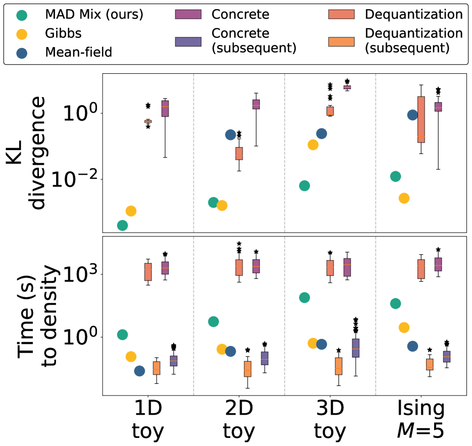
(a) Normalized target

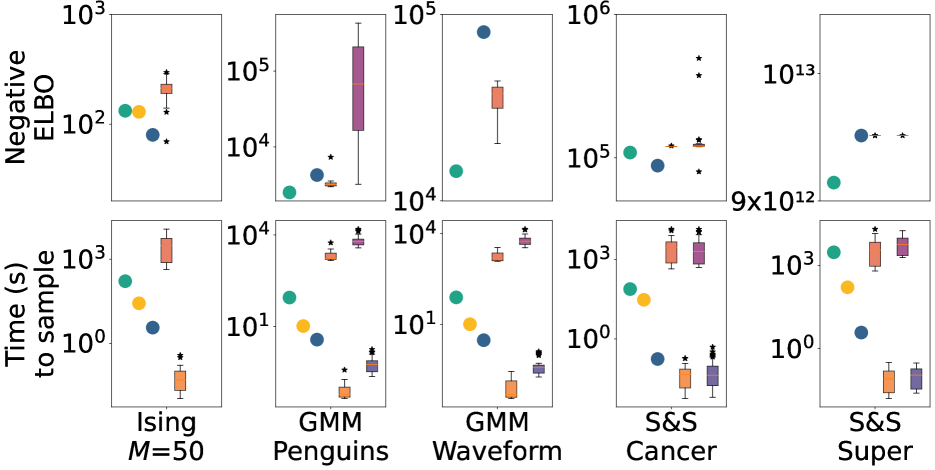
(b) Unnormalized target

Figure 2: Summary of experiments. In Fig. 2(a), the normalizing constant $Z$ of the target density is known and in Fig. 2(b) $Z$ is not tractable. The boxplots for continuous-embedding flows represent the search over different architecture settings. (Top row): KL divergence (Fig. 2(a)) and negative ELBO (Fig. 2(b)) from approximation to target distribution. Lower is better. (Bottom row): Compute time (seconds) to evaluate or estimate the density (Fig. 2(a)) or to generate a sample (Fig. 2(b)). The second set of boxplots for continuous-embedding flows show the time to evaluate a subsequent density point after training. Missing values indicate either that the algorithm cannot be used for that task or that it was too computationally unstable to produce results, except for 1D mean-field VI which produces exact results ($\mathrm{KL}=0$). Colors are shared across figures and $x$-axes across columns.

Fig. 2 presents a summary of our experiments. MAD Mix obtains good approximations across the board at a fraction of the compute cost of dequantization and Concrete-relaxed flows. The time plot includes the time necessary to train all the flows in the architecture search. Since training the flow is a computational bottleneck, we also show a separate set of boxplots for the time required to evaluate the density of the approximation after training. This shows that, although density evaluation is computationally cheap given a trained flow, optimization can be costly and should be accounted for in the compute budget. We also found that Concrete-relaxed flows were prone to numerical instability and could not always be inverted for density evaluation in more complex examples, as shown by their omission in Fig. 2(b). This behaviour has been documented in the past (e.g., Dinh et al., 2017, Sec. 3.7). Gibbs sampling and mean-field VI require less compute time to sample or to evaluate a density than MAD Mix; see the bottom plots of Figs. 2(a) and 2(b). However, the former struggles to produce high-quality approximations in complex examples and the latter does not provide access to the density of the approximation. This is shown in Fig. 2(b), where the ELBO could not be estimated for Gibbs sampling.

4.1 Discrete toy examples

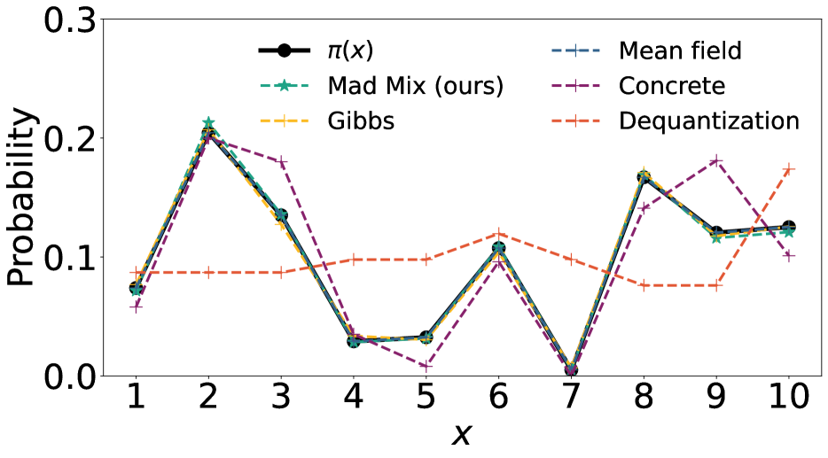
(a) 1D PMF

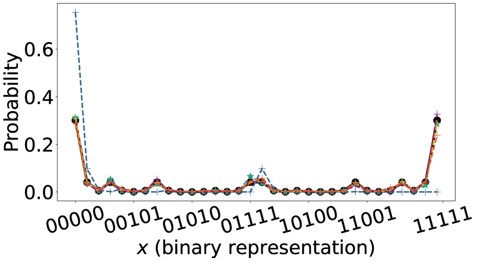
(b) Ising $M=5$ flattened PMF

(c) 2D $x_{1}$-marginal PMF

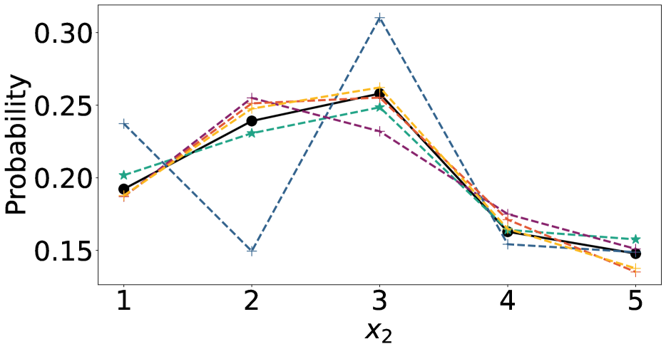
(d) 2D $x_{2}$-marginal PMF

Figure 3: True and approximated PMFs of the 1D, 2D, and low-dimensional Ising examples. For the Ising model, we treat each $x\in\mathcal{X}$ as an element of $\{0,1\}^{M}$ (i.e., a binary representation) and show the flattened PMF in ascending order of binary representation. The legend is shared across figures.

First we consider three discrete toy examples: a 1D distribution on $\{1,\dots,10\}$, a 2D distribution on $\{1,\dots,4\}\times\{1,\dots,5\}$, and a 3D distribution on $\{1,\cdots,10\}^{3}$. In all cases, MAD Mix produces a high-fidelity approximation of the target distribution as seen in Figs. 2(a) and 3. Concrete-relaxed flows produce good global approximations but generally fail to recover the local shape. This results in small but not negligible KL to the target, as seen in Fig. 2. Dequantization generally produces better approximations than Concrete, but it failed to properly capture the shape of the simplest, 1D toy example (see Fig. 3(a)). This behaviour was consistent across all architecture configurations, and a visual inspection of the loss traceplots suggests that the optimizer converged in all cases. Gibbs sampling and mean-field VI were computationally cheaper than MAD Mix but they generally produced approximations with higher KL to the target. In contrast, continous-embedding flows consistently require more compute and produce, on average, worse approximations.

4.2 Ising model

Next, we consider an Ising model on $\mathcal{X}=\{-1,+1\}^{M}$ with log-PMF $\log\pi(x)=\beta\sum_{m=1}^{M-1}x_{m}x_{m+1}-\log Z$, where $\beta>0$ is the inverse temperature and $M$ controls the dimension of the problem. The normalizing constant $Z$ involves a sum over $2^{M}$ terms (equal to the dimension of the latent space) but the full conditionals $\pi_{m}$ can be calculated in closed form for any $M$. We considered a small $M$ and a large $M$ setting, with dimensions $M=5$ and $M=50$ and inverse temperatures $\beta=1$ and $\beta=5$, respectively. In the $M=5$ case, the normalizing constant can be computed. All methods except mean-field (due to the $M$ particles being treated as independent) produce high-fidelity approximations; see Fig. 3(b). However, only a few continuous-embedding flow architectures resulted in small KL divergences, as seen in Fig. 2(a). The implementation in PyTorch (Paszke et al., 2019) of Concrete relaxations requires access to all the (possibly unnormalized) probabilities. Since allocating a vector of size $2^{50}$ is not possible, we were unable to fit a Concrete-relaxed flow in the $M=50$ setting. As seen in Fig. 2(b), MAD Mix, dequantization, mean-field VI, and Gibbs sampling all perform comparably. The ELBO estimates for Gibbs sampling and dequantization were obtained via empirical frequency PMF estimators (the former since Gibbs does not provide access to densities, the latter since one needs to approximate an $M$-dimensional integral to estimate the PMF, which is not feasible for large $M$). In contrast, both MAD Mix and mean-field VI provide access to exact PMF evaluation.

4.3 Gaussian mixture model

To showcase a joint continuous and discrete example, we considered a Gaussian mixture model (GMM) with likelihood $\sum_{k=1}^{K}w_{k}\phi_{\mu_{k},\Sigma_{k}}$, where $w\in\Delta^{K-1}$ and $\phi_{\mu,\Sigma}$ is a Gaussian distribution with mean $\mu$ and covariance matrix $\Sigma$. We fit this model to two datasets: the Palmer penguins dataset and the waveform dataset. The former has 333 observations of four different measurements of three species of penguins and the latter contains 300 simulated observations of 21 measurements of three classes. Following Hastie et al. (2009), we use the first two principal components of the measurements as the observations. In both examples, we perform inference over the labels, the weights, and the measurement means and covariance matrices of each species (penguins) and class (waveform), for total latent space dimensions of 1044 for the penguins data and 918 for the waveform data. See Appendix E for specific modeling details. We fit the mixed discrete-continuous variant of MAD Mix described in Section 3.5. Fig. 2(b) shows the results of both data sets. Gibbs cannot produce an estimate of the ELBO and so we are unable to assess its accuracy. We also noticed that most of the architecture configurations for both continuous-embedding methods resulted in gradient overflow. Furthermore, the few Concrete flows in the waveform data set that were successfully trained produced covariance matrices whose diagonal was (numerically) zero. Evaluating the target density to then estimate the ELBO was therefore not possible. From Fig. 2(b), MAD Mix produces approximations with a higher ELBO than mean-field VI, dequantization, and Concrete-relaxed flows.

4.4 Spike-and-Slab model

Finally, we considered a sparse Bayesian regression experiment where we modeled $N$ observations $y_{n}\sim\mathcal{N}(\beta^{\top}x_{n},\sigma^{2})$ and placed a spike-and-slab prior on the $P$ regression coefficients: $\beta_{p}\sim(1-\gamma_{p})\delta_{0}+\gamma_{p}\mathcal{N}(0,\nu^{2})$ for all $p$. See Appendix F for more modeling details. We fit this model to two datasets: a pancreatic cancer dataset with $N=97$ and $P=8$ and a superconductivity dataset with $N=100$ (subsampled) and $P=81$. We performed inference on the coefficients $\beta_{p}$, the binary variables $\gamma_{p}\in\{0,1\}$ that indicate whether $\beta_{p}=0$ or not, and the variances $\sigma^{2},\nu^{2}$. The latent space dimensions are 27 for the cancer data set and 246 for the superconductivity data set. From Fig. 2(b), MAD Mix performs comparably to continuous-embedding flows (although the largest ELBO was produced by a single Concrete-relaxed architecture configuration) and slightly underperforms compared to mean-field VI in the cancer data set. In the higher dimensional superconductivity data set, however, MAD Mix outperforms all the competitors (albeit at a larger compute cost). Again, we cannot compute the ELBO for Gibbs sampling, but we expect it to behave similarly to MAD Mix.

5 Conclusion

In this work we introduced MAD Mix, a new variational family to learn discrete distributions without embedding them in continuous spaces. MAD Mix consists of a mixture of repeated applications of a novel Measure-preserving And Discrete (MAD) map that generalizes those used by deterministic MCMC samplers. Our experiments show that MAD Mix produces high-fidelity approximations at a fraction of the compute cost (including training) than those obtained from continuous-embedding normalizing flows. Since MAD Mix mimics sequentially sampling from the target’s full conditionals, the quality of the approximation in the discrete setting will depend on the mixing properties of Gibbs sampling. Future work can explore new measure-preserving and ergodic maps that lead to flow-based families like MAD Mix but with better mixing.

Appendix A Implementation details

MAD Mix

There are two tunable parameters in MAD Mix: the vertical shift $\xi$ in Step (2) and the number $N$ of repeated applications of $T_{\mathrm{MAD}}$. Following Xu et al. (2023), we fixed $\xi=\pi/16$ and found that it worked well in all our cases. We chose $N$ to achieve a desirable tradeoff between the accuracy of the approximation $q_{N}$ (measured by the ELBO) and the time it took to evaluate the density of or generate samples from $q_{N}$. We found that $N$ in the order of $10^{2}$ was sufficient for all of our experiments, and specifically we set $N=500$ for the univariate and bivariate toy examples, $N=100$ for the 3D toy example, $N=1000$ for the low-dimensional Ising example and $N=500$ for the high-dimensional one, $N=100$ for both Gaussian mixture models, and $N=500$ for both Spike-and-Slab examples. $N$ can be thought of as the number of Gibbs sampling steps being averaged over (since the MAD map mimics a deterministic Gibbs sampler).

Normalizing flow architecture

We conducted a search over 144 different setting configurations for Concrete-relaxed normalizing flows and 36 different settings for dequantization-based flows. Our motivation was to reflect the effort of tuning continuous-embedding flows in practice by searching over reasonable configuration attempts.

For our base architecture, we considered a Real NVP normalizing flow (Dinh et al., 2017), which has been shown to provide highly expressive approximations to continuous distributions. Each pass of a Real NVP flow transforms $x\mapsto x^{\prime}$ and is constructed by scaling and translating only some of the inputs:

$$x=[x_{a},x_{b}],\quad x_{a}^{\prime}=\exp(s(x_{b};\psi_{s}))\odot x_{a}+t(x_{b};\psi_{t}),\quad x^{\prime}:=[x_{a}^{\prime},x_{b}],$$ (22)

where $s$ and $t$ are neural networks that depend on $x_{b}$ and parameters $\psi=(\psi_{s},\psi_{t})$ and $\odot$ indicates element-wise multiplication. We defined $s$ and $t$ by composing three applications of a single-layer linear feed forward neural network with leaky ReLU activation functions in between. For the scale transformation $s$, we added a hyperbolic tangent layer too:

$$t(x_{b};\psi_{t}) =(\mathrm{Linear}\circ\mathrm{ReLU}\circ\mathrm{Linear}\circ\mathrm{ReLU}\circ\mathrm{Linear})(x_{b};\psi_{t}),$$ (23)

$$s(x_{b};\psi_{s}) =(\tanh\circ\mathrm{Linear}\circ\mathrm{ReLU}\circ\mathrm{Linear}\circ\mathrm{ReLU}\circ\mathrm{Linear})(x_{b};\psi_{s}).$$ (24)

The initial and final widths of $s$ and $t$ (i.e., the first and last Linear layers in $t$ and the first Linear and the hyperbolic tangent layers in $s$) were chosen to match the dimension of $x$. For example, in the 1D toy discrete example, the dimension of the Concrete-relaxed $x$ is 10 because the underlying discrete random variable takes values in $\{1,\dots,10\}$. For the intermediate layers, we considered four different widths: 32, 64, 128, and 256.

These steps define a single pass of the Real NVP map, but in practice it is necessary to do multiple passes (the number of which is the depth of the flow). We considered three different depths: 10, 50, and 100. To increase the expressiveness of the flow, we alternated between updating the first half and the last half of the inputs in each pass (as recommended by Dinh et al. (2017)). That is, on odd passes $x_{a}$ in Eq. 22 would correspond to the first half of $x$ and on even passes to the last half of $x$.

Additionally, for Concrete-relaxed flows we considered multiple possible values of the temperature parameter $\lambda$ that controls the fidelity of the relaxation: when $\lambda\to 0$, the relaxed distribution converges to the original discrete distribution, but this in turn causes the relaxation to be “peaky” near the vertices of the simplex and therefore gradients are numerically unstable. Based on the discussion in Maddison et al. (2017, Appendix C.4), we considered four different temperatures: 0.1, 0.5, 1, and 5. This range covers different approximation quality/computational stability tradeoff regimes and covers the optimal values found by Maddison et al. (2017) in their experiments. For the multivariate distributions, we instead relaxed a “flattened” target distribution with dimension equal to the product of the dimensions of each variable. E.g., we mapped the bivariate toy example with values in $\{1,\dots,5\}\times\{1,\dots,4\}$ to a univariate distribution with values in $\{1,\dots,20\}$.

We implemented the Real NVP normalizing flow (both for Concrete relaxations and for dequantization) in PyTorch (Paszke et al., 2019). In practice, we used a log-transformed Concrete approximation as suggested in Maddison et al. (2017, Appendix C.3), which we found to be more numerically stable. We learned the parameters of the flow by running Adam (Kingma and Ba, 2015) for 10,000 iterations. We considered three different learning rates: $10^{-5}$, $10^{-3}$, and $10^{-1}$.

We optimized all flows in parallel using Sockeye (UBC Advanced Research Computing, 2023), a high-performance computing platform at our institution.

Appendix B PMF of approximations of toy examples

Appendix C MAD Mix KL-optimal weighting

One of the main benefits of MAD Mix over Gibbs sampling and other stochastic MCMC samplers is having access to density estimates of the approximation. Combined with the availability of i.i.d. samples, this allows us to estimate the ELBO and therefore to optimally weight two different MAD Mix flows, each initialized in a different reference distribution. This is useful, for example, when we know where certain high posterior mass regions are but a usual MCMC sampler would struggle to mix between them. Here we consider the case where there are two such regions, but this can be extended to an arbitrary number. Formally, we consider a variational proposal of the form

$$q_{N}=wq_{N,0}+(1-w)q_{N,1},$$ (25)

where $w\in(0,1)$, $q_{N,i}=\frac{1}{N}\sum_{n=0}^{N-1}T_{\mathrm{MAD}}^{n}q_{i}$, and $q_{i}$ is a reference distribution that covers the region $i$, $i=0,1$. We then select

$$w=\arg\min_{\alpha\in(0,1)}\mathrm{D}_{\mathrm{KL}}(\alpha q_{N,0}+(1-\alpha)q_{N,1}\,||\,\pi),$$ (26)

which can be estimated via gradient descent since

$$\frac{\mathrm{d}}{\mathrm{d}\alpha}\mathrm{D}_{\mathrm{KL}}(\alpha q_{N,0}+(1-\alpha)q_{N,1}\,||\,\pi)=\mathbb{E}_{q_{N,0}}\left[\log\frac{\alpha q_{N,0}+(1-\alpha)q_{N,1}}{\pi}\right]-\mathbb{E}_{q_{N,1}}\left[\log\frac{\alpha q_{N,0}+(1-\alpha)q_{N,1}}{\pi}\right].$$ (27)

In practice, one can generate samples from $q_{N,0}$ and $q_{N,1}$ and use them to estimate the expectations.

Appendix D Ising model details

Recall that the Ising model has target density

$$\pi(x)\propto\exp\left\{\beta\sum_{m=1}^{M-1}x_{m}x_{m+1}\right\}$$ (28)

with $\beta>0$ the inverse temperature and $x\in\{-1,+1\}^{M}=\mathcal{X}$. The full conditionals can be found in closed form by analyzing only the terms affecting each particle’s immediate neighbors. For the particles $x_{1}$ and $x_{M}$ the full conditional only depends on their single neighbor:

$$\pi_{1}(x)=\frac{\exp(\beta xx_{2})}{2\cosh(\beta)},\qquad\pi_{M}(x)=\frac{\exp(\beta xx_{M-1})}{2\cosh(\beta)}.$$ (29)

The normalizing constant is tractable since it involves adding two terms and can be simplified since $\cosh(\beta)=\cosh(-\beta)$. The probability for particles with two neighbors $x_{m},1<m<M$, is likewise given by

$$\pi_{m}(x)=\frac{\exp(\beta x(x_{m-1}+x_{m+1}))}{2\cosh(\beta(x_{m-1}+x_{m+1}))}.$$ (30)

Appendix E Gaussian mixture model experiment details

We use the labels $x_{1:N}$ to rewrite the likelihood as a product over the sample and label indices:

$$\ell(y_{1:N};x_{1:N},w_{1:K},\mu_{1:K},\Sigma_{1:K})=\prod_{n=1}^{N}\prod_{k=1}^{K}(w_{k}\phi_{\mu_{k},\Sigma_{k}}(y_{n}))^{\mathbb{I}(x_{n}=k)},$$ (31)

where $\phi_{\mu,\Sigma}(y)$ is the density of a $\mathcal{N}(\mu,\Sigma)$ distribution evaluated at $y\in\mathbb{R}^{D}$.

We considered uninformative and independent prior distributions for each of the $NK+3K$ parameters:

$$X_{n}\mid w \sim\mathrm{Categorical}(w_{1},\dots,w_{K}),\quad n\in[N]$$ (32)

$$w \sim{\sf{Dir}}(\alpha_{1},\dots,\alpha_{K}),$$ (33)

$$\mu_{k}\mid\Sigma_{k} \sim\mathcal{N}(m_{0,k},\Sigma_{k}),\quad k\in[K]$$ (34)

$$\Sigma_{k} \sim\mathpzc{IW}(S_{0,k},\nu_{0,k}),\quad k\in[K].$$ (35)

We set $\alpha_{k}=1$ for all $k$, reflecting little prior knowledge of the weights. We also set $\nu_{0,k}=1$ and chose $m_{0,k}$ and $S_{0,k}$ by visually inspecting the data for all $k$. We initialized MAD Mix, the Gibbs sampler, and the mean-field algorithm at these values for fairness.

These prior distribution are conjugate and the full conditionals can be found in closed form:

$$X_{n}\mid w,\mu_{1:K},\Sigma_{1:K} \sim{\sf{Categorical}}(w_{1}\phi_{\mu_{1},\Sigma_{1}}(y_{n}),\dots,w_{K}\phi_{\mu_{K},\Sigma_{K}}(y_{n})),\quad n\in[N],$$ (36)

$$w\mid X_{1:N} \sim{\sf{Dir}}(\alpha_{1}+N_{1},\dots,\alpha_{K}+N_{K}),\quad k\in[K],$$ (37)

$$\mu_{k}\mid\Sigma_{k},X_{1:N} \sim\mathcal{N}(\bar{y}_{k},\Sigma_{k}/N_{k}),\quad k\in[K],$$ (38)

$$\Sigma_{k}\mid X_{1:N} \sim\mathpzc{IW}(S_{k},N_{k}-D-1),\quad k\in[K].$$ (39)

Above, $D$ is the dimension of the data, $N_{k}=\sum_{n}\mathds{1}(x_{n}=k)$ is the number of elements in cluster $k$, $\bar{y}_{k}=N_{k}^{-1}\sum_{n}y_{n}\mathds{1}(x_{n}=k)$ is the mean of elements in cluster $k$, and $S_{k}=\sum_{n}(y_{n}-\bar{y}_{k})(y_{n}-\bar{y}_{k})^{\top}\mathds{1}(x_{n}=k)$ the corresponding scaled covariance. The mean-field algorithm also has closed-form updates; we followed Bishop (2006, Sec. 10.2).

MAD Mix implementation

For the deterministic Hamiltonian move, we need the score function of the parameters $(w,\mu_{1:K},\Sigma_{1:K})$. Note that the score w.r.t. the weights will only depend on $p(w)$ and the score w.r.t. the $k$th mean will only depend on $p(\mu_{k}\,|\,\Sigma_{k})$.

The score w.r.t. the weights is then

$$\nabla_{w}\log p(w,\mu,\Sigma)=\nabla_{w}\log p(w)=\nabla_{w}\sum_{k}N_{k}\log w_{k}=\left(\frac{N_{1}}{w_{1}},\dots,\frac{N_{K}}{w_{K}}\right)^{\top}.$$ (40)

The score w.r.t. the $k$th mean is

$$\nabla_{\mu_{k}}\log p(w,\mu,\Sigma)=\nabla_{\mu_{k}}\log p(\mu_{k}\,|\,\Sigma)=-N_{k}\Sigma_{k}^{-1}(\mu_{k}-\bar{y}_{k}).$$ (41)

Finally, the score w.r.t. the $k$th covariance depends on both the mean PDF and the covariance PDF:

$$\nabla_{\Sigma_{k}}\log p(w,\mu,\Sigma)=\nabla_{\Sigma_{k}}\log p(\mu_{k}\,|\,\Sigma_{k})+\log p(\Sigma_{k}).$$ (42)

The first term is

$$\nabla_{\Sigma_{k}}\log p(\mu_{k}\,|\,\Sigma_{k})=-\frac{1}{2}\Sigma_{k}^{-\top}-\frac{N_{k}}{2}(\mu_{k}-\bar{y}_{k})(\mu_{k}-\bar{y}_{k})^{\top},$$ (43)

where we used the identities $\partial\log|X|=X^{-\top}$ and $\partial a^{\top}Xb=ab^{\top}$ (Petersen and Pedersen, 2008). The second term is

$$\nabla_{\Sigma_{k}}\log p(\Sigma_{k})=-\frac{N_{k}}{2}\Sigma_{k}^{-\top}+\frac{1}{2}\left(\Sigma_{k}^{-1}S_{k}\Sigma_{k}^{-1}\right)^{\top},$$ (44)

where we used the identity $\partial\mathrm{tr}(AX^{-1}B)=-X^{-\top}A^{\top}B^{\top}X^{-\top}$ (Petersen and Pedersen, 2008). Adding together these two expressions yields the score w.r.t. the $k$th covariance:

$$\nabla_{\Sigma_{k}}\log p(w,\mu,\Sigma)=-\frac{1}{2}(1+N_{k})\Sigma_{k}^{-\top}-\frac{N_{k}}{2}(\mu_{k}-\bar{y}_{k})(\mu_{k}-\bar{y}_{k})^{\top}+\frac{1}{2}\left(\Sigma_{k}^{-1}S_{k}\Sigma_{k}^{-1}\right)^{\top}.$$ (45)

In practice, we avoid working with the covariance matrix directly since it has to be symmetric and positive definite, and taking Hamiltonian steps can make the resulting matrix inadmissible. Instead, given a covariance matrix $\Sigma$, let $\Sigma=LL^{\top}$ be its (unique) Cholesky decomposition. The matrix $L$ is lower triangular and has positive diagonal elements, and hence we only need to store the $D+\binom{D}{2}$ non-zero elements. To further remove the positiveness condition, define $H$ as a copy of $L$ but with the diagonal log-transformed:

$$H_{ij}=\begin{cases}0,&i<j,\\ \log L_{ij},&i=j,\\ L_{ij},&i>j.\end{cases}$$ (46)

By taking steps in $H$-space, we are guaranteed to get back a valid covariance matrix. To map from $H$ to $\Sigma$, we exp-transform the diagonal to get $L$ and then set $\Sigma=LL^{\top}$. Let $f$ be the function that maps $\Sigma$ to $H$, so that $f(\Sigma)=H$. The Jacobian of the transformation can be found in closed-form and the resulting log density is

$$\log p(H)=\log p(\Sigma)+\sum_{d=1}^{D}(D-d+2)H_{dd}+D\log 2,$$ (47)

where $D$ is the dimension of observations (Njoroge, 1988, Theorem 4.2).

To take a Hamiltonian step in $H$ space, however, we need $\nabla_{H}\log p(H)$. We take the gradient w.r.t. $H$ in Eq. 47. The third term does not depend on $H$. The gradient of the second term is a diagonal matrix with the $d$th diagonal entry equal to $D-d+2$. Using the chain rule, the gradient of the first term is

$$\nabla_{H}\log p_{\Sigma}(f^{-1}(H))=\nabla_{H}f^{-1}(H)\nabla_{\Sigma}\log p_{\Sigma}(f^{-1}(H)).$$ (48)

The second factor is equal to $\nabla_{\Sigma}\log p_{\Sigma}(\Sigma)$, which we derived in Eq. 45, since $\Sigma=f(H)$. The first factor is the Jacobian of the inverse transform $f$. Note that this is a $D^{2}\times D^{2}$ matrix, so the second factor should be understood as a $D^{2}$ vector (a flattened matrix). We find this matrix by computing the Jacobian matrix of the transform from $H$ to $L$, say $J_{1}$, and multiplying it with the corresponding Jacobian of the map from $L$ to $LL^{\top}=\Sigma$, $J_{2}$. The first Jacobian matrix $J_{1}$ is diagonal with entries either 1 or $\exp(H_{dd})$. Specifically,

$$J_{1}=\mathrm{Diag}(\exp(H_{11}),1,\dots,1,\exp(H_{22}),1,\dots,1,\exp(H_{DD}),1,\dots,1).$$ (49)

For $J_{2}$, we introduce the $D^{2}\times D^{2}$ commutation matrix $K_{D}$. If $A$ is a $D\times D$ matrix denote by $\mathrm{vec}(A)$ the vectorized or flattened version of $A$, i.e., the $\mathbb{R}^{D^{2}}$ vector obtained by stacking the columns of $A$ one after the other. Then $K_{D}$ satisfies that $K_{D}\mathrm{vec}(A)=\mathrm{vec}(A^{\top})$ and we have

$$J_{2}=\frac{\partial\mathrm{vec}(LL^{\top})}{\partial\mathrm{vec}(L)}=(L\otimes I_{D})+(L\otimes I_{D})K_{D},$$ (50)

where $\otimes$ is the Kroenecker product and $I_{D}$ is the $D\times D$ identity matrix. Finally, $\nabla_{H}f^{-1}(H)=J_{2}J_{1}$. We also use this decomposition for all the continuous-embedding flows.

Appendix F Spike-and-Slab model details

We consider $N$ real-valued observations $y_{1:N}$ with accompanying $P$ covariates $x_{n}\in\mathbb{R}^{P}$, which we stack horizontally in a design matrix $X\in\mathbb{R}^{N\times P}$. We assume a linear regression setting where

$$y_{n}\sim\mathcal{N}(\beta^{\top}x_{n},\sigma^{2}),$$ (51)

with regression coefficients $\beta\in\mathbb{R}^{P}$ and unknown variance $\sigma^{2}$. To induce sparseness in $\beta$, we introduce additional latent variables $\theta\in(0,1)$, $\gamma_{1:P}\in\{0,1\}^{P}$, and $\tau^{2}>0$, and consider the following hierarchical model:

$$\tau^{2} \sim{\sf{InvGam}}(\alpha_{1},\alpha_{2}),$$ (52)

$$\sigma^{2} \sim{\sf{Gam}}(\frac{1}{2},\frac{s^{2}}{2}),$$ (53)

$$\theta \sim{\sf{Beta}}(a,b),$$ (54)

$$\gamma_{p} \sim{\sf{Categorical}}(1-\theta,\theta),\qquad p=1,\dots,P,$$ (55)

$$\beta_{p} \sim(1-\gamma_{p})\delta_{0}+\gamma_{p}\mathcal{N}(0,\sigma^{2}\tau^{2}),\qquad p=1,\dots,P,$$ (56)

where $\delta_{0}$ is a Dirac delta at 0. The variance of the regression coefficients $\nu^{2}=\sigma^{2}\tau^{2}$ depends on both the variance of the observations $\sigma^{2}$ and on $\tau^{2}$ to allow the prior to scale with the scale of the observations. We set $\alpha_{1}=\alpha_{2}=0.1$, $s^{2}=0.5$, and $a=b=1$ to reflect little prior knowledge about the latent variables. We initialized the regression coefficients in MAD Mix, Gibbs sampling, and mean-field VI at the least-squares estimator.

These prior distributions are conjugate and the full conditionals can be found in closed form:

$$\tau^{2}\mid\sigma^{2},\beta,\gamma_{1:P}, \sim{\sf{InvGam}}\left(\frac{1}{2}+\frac{1}{2}\sum_{p=1}^{P}\gamma_{p},\frac{s^{2}}{2}+\frac{\beta^{\top}\beta}{2\sigma^{2}}\right),$$ (57)

$$\sigma^{2}\mid y,\beta \sim{\sf{Gam}}\left(\alpha_{1}+\frac{N}{2},\alpha_{2}+\frac{1}{2}(y-X\beta)^{\top}(y-X\beta)\right),$$ (58)

$$\theta\mid\gamma_{1:P} \sim{\sf{Beta}}\left(a+\sum_{p=1}^{P}\gamma_{p},b+P-\sum_{p=1}^{P}\gamma_{p}\right),$$ (59)

$$\beta\mid y,\gamma_{1:P},\tau^{2},\sigma^{2} \sim\mathcal{N}\left(\frac{1}{\sigma^{2}}HX^{\top}y,H\right),$$ (60)

$$\gamma_{p}\mid\beta,\theta,\tau^{2},y \sim{\sf{Categorical}}(1-\xi_{p},\xi_{p}),$$ (61)

where $H=\sigma^{2}(X^{\top}X+\frac{1}{\tau^{2}}I_{P})^{-1}$ is the projection matrix in ridge regression (sans an additional $X^{\top}$ term). The Categorical probabilities for the full conditional of $\gamma_{p}$ are given by

$$1-\xi_{p}=\frac{1-\theta}{\tau^{-1}\exp\left(\frac{\left(\sum_{n=1}^{N}x_{n}^{\top}z_{p}\right)^{2}}{2\sigma^{2}\left(\sum_{n=1}^{N}x_{n}^{\top}x_{n}+\frac{1}{\tau^{2}}\right)}\right)\left(\sum_{n=1}^{N}x_{n}^{\top}x_{n}+\frac{1}{\tau^{2}}\right)^{-1/2}\theta+(1-\theta)},$$ (62)

where $z_{p}=y-X\beta_{-p}$ are the residuals from the model with parameters $\beta_{-p}$ in which we set $\beta_{p}=0$. The derivations can be found in Dablander (2019). For mean-field VI, we followed Ray and Szabó (2022) and used their software (Clara et al., 2021).

MAD Mix implementation

In practice, we transform the restricted variables $\theta\in(0,1),\sigma^{2},\tau^{2}>0$ into real-valued parameters to prevent the Hamiltonian dynamics from resulting in unfeasible values. Specifically, we reparametrize

$$\theta_{u}=\log\frac{\theta}{1-\theta},\quad\tau_{u}^{2}=\log\tau^{2},\quad\sigma_{u}^{2}=\log\sigma^{2}.$$ (63)

These transformations are bijective and have Jacobians

$$J_{\theta_{u}}=\frac{1}{\theta(1-\theta)},\quad J_{\tau_{u}^{2}}=\frac{1}{\tau^{2}},\quad J_{\sigma_{u}^{2}}=\frac{1}{\sigma^{2}}.$$ (64)

We do inference over the unrestricted parameters and also use them for Concrete-relaxed flows and dequantization.

As with the GMM experiment, we need the score functions of the continuous variables for the Hamiltonian step in MAD Mix. Let $\pi$ denote the spike-and-slab posterior distribution as a function of the continuous variables only (see Section 3.2 for more details). Then the score functions are given by

$$\nabla_{\theta_{u}}\log\pi(\theta_{u},\sigma_{u}^{2},\tau_{u}^{2},\beta;\gamma_{1:P}) =\frac{a-1}{\theta}-\frac{b-1}{\theta}-\frac{1}{\theta(1-\theta)},$$ (65)

$$\nabla_{\tau_{u}^{2}}\log\pi(\theta_{u},\sigma_{u}^{2},\tau_{u}^{2},\beta;\gamma_{1:P}) =\frac{s^{2}}{2(\tau^{2})^{2}}-\frac{1+\sum_{p=1}^{P}\gamma_{p}}{2\tau^{2}}+\frac{1}{2\sigma^{2}\tau^{2}}\sum_{p=1}^{P}\gamma_{p}\beta_{p}^{2},$$ (66)

$$\nabla_{\sigma_{u}^{2}}\log\pi(\theta_{u},\sigma_{u}^{2},\tau_{u}^{2},\beta;\gamma_{1:P}) =\frac{2\alpha_{2}+(y-X\beta)^{\top}(y-X\beta)}{2(\sigma^{2})^{2}}-\frac{2\alpha_{1}+N+\sum_{p=1}^{P}\gamma_{p}}{2\sigma^{2}}+\frac{1}{2\sigma^{2}\tau^{2}}\sum_{p=1}^{P}\gamma_{p}\beta_{p}^{2},$$ (67)

$$\nabla_{\beta}\log\pi(\theta_{u},\sigma_{u}^{2},\tau_{u}^{2},\beta;\gamma_{1:P}) =\frac{1}{\sigma^{2}}\left(X^{\top}y-X^{\top}X\beta-\frac{1}{\tau^{2}}\beta\right).$$ (68)

Appendix G Proofs

First we state and prove a series of results that will be helpful in the proof of Proposition 3.1.

G.1 Derivative under modulo operation

To calculate the density of the pushfoward under $T_{\mathrm{MAD}}$, we need to calculate the derivative of the modulo operation. Lemma G.1 below shows that the update $\rho\mapsto\rho^{\prime}$ in Step (2) of the MAD map has unit derivative.

Lemma G.1.

Let $\rho\in(0,1)$ and define $\rho^{\prime}=\rho+\xi\mod 1$, where $\xi\in\mathbb{R}$. Then the transformation $\rho\mapsto\rho^{\prime}$ has unit derivative:

$$\frac{\mathrm{d}\rho^{\prime}}{\mathrm{d}\rho}=1\qquad\rho+\xi\mod 1\neq 0.$$ (69)

If $\rho+\xi\mod 1=0$ then the derivative is not defined.

Proof of Lemma G.1.

We can rewrite the modulo function as the original value minus the integer part of the remainder:

$$\rho+\xi\mod 1=\rho+\xi-\lfloor\rho+\xi-1\rfloor.$$ (70)

When taking derivative w.r.t. $\rho$, the term $\rho+\xi$ has unit derivative and the floor term has derivative zero since the floor function is piecewise constant in $(0,1)$. ∎

G.2 Change of variables for joint discrete and continous transformations

The usual change of variables formula is valid when all the variables are continuous (e.g., Eq. 4) or when all the variables are discrete (in which case there is no Jacobian term). In this section, we develop an analogue for the case where some variables are discrete and some are continuous. We consider the setting where a base distribution $\pi_{0}$ has exactly one discrete and one continuous component, but the result generalizes. Formally, let $\pi_{0}$ be a density on $\mathbb{N}\times\mathbb{R}$, $T:\mathbb{N}\times\mathbb{R}\to\mathbb{N}\times\mathbb{R}$ be an invertible transformation where $T(n,x)=(T_{\mathrm{d}}(n,x),T_{\mathrm{c}}(n,x))$, and $\pi_{1}=T\pi_{0}$ be the pushforward of $\pi_{0}$ under $T$. Throughout, we consider two assumptions:

• The map $T$ is invertible.

• For all $n\in\mathbb{N}$, the map $T_{\mathrm{c}}(n,\cdot)$ is invertible.

First we introduce some notation that will be useful to prove the main result.

Lemma G.2.

Define

$$A_{nm}=\left\{x\in\mathbb{R}\mid T_{\mathrm{d}}(n,x)=m\right\},\qquad B_{nm}=\{y\in\mathbb{R}\mid y=T_{\mathrm{c}}(n,x),\,x\in A_{nm}\},\qquad n,m\in\mathbb{N}.$$ (71)

Then, under Assumptions (A1) and (A2), for any fixed $n\in\mathbb{N}$ the $(A_{nm})_{m=1}^{\infty}$ are a partition of $\mathbb{R}$ and, for any fixed $m\in\mathbb{N}$, the $(B_{nm})_{n=1}^{\infty}$ are a partition of $\mathbb{R}$.

Proof of Lemma G.2.

For all $n\in\mathbb{N}$, each $x\in\mathbb{R}$ is in one of the sets $(A_{nm})_{m\in\mathbb{N}}$: the one for which $T_{\mathrm{d}}(n,x)=m$. Therefore for any fixed $n$ the $(A_{nm})_{m}$ are disjoint and cover all of $\mathbb{R}$.

To show disjointness of the $(B_{nm})_{n}$, suppose that $y\in B_{nm}\cap B_{n^{\prime}m}$ for $n\neq n^{\prime}$. Then by definition there would exist $x\in A_{nm},x^{\prime}\in A_{n^{\prime}m}$ such that $T_{\mathrm{c}}(n,x)=y=T_{\mathrm{c}}(n^{\prime},x^{\prime})$. But since $x,x^{\prime}$ belong to $A_{nm}$ and $A_{n^{\prime}m}$ (respectively), $T_{\mathrm{d}}(n,x)=m=T_{\mathrm{d}}(n^{\prime},x^{\prime})$. Hence $T(n,x)=T(n^{\prime},x^{\prime})$ and thus $(n,x)=(n^{\prime},x^{\prime})$ because $T$ is invertible, which is a contradiction since we assumed $n\neq n^{\prime}$. To show that the $(B_{nm})_{n}$ cover $\mathbb{R}$ for a fixed $m$, given $y\in\mathbb{R}$ let $(n,x)=T^{-1}(m,y)$, i.e., $T_{\mathrm{d}}(n,x)=m$ and $T_{\mathrm{c}}(n,x)=y$. The first equality implies $x\in A_{nm}$, which together with the second equality shows $y\in B_{nm}\subseteq\cup_{n}B_{nm}$. ∎

Now we state the main result.

Proposition G.3.

Let $J_{\mathrm{c}}$ be the conditional Jacobian w.r.t. the continous variable $x$ of the map $T_{\mathrm{c}}(n,\cdot)$, and let $J_{\mathrm{c}}^{-1}$ be the Jacobian of the inverse map:

$$J_{\mathrm{c}}(n,x):=\frac{\mathrm{d}T_{\mathrm{c}}(n,\cdot)}{\mathrm{d}x}\Bigg{|}_{x},\qquad J_{\mathrm{c}}^{-1}(n,x):=\frac{\mathrm{d}T_{\mathrm{c}}^{-1}(n,\cdot)}{\mathrm{d}y}\Bigg{|}_{y=T_{\mathrm{c}}(n,x).}$$ (72)

Then under Assumptions (A1) and (A2), the density of the pushforward $\pi_{1}$ is given by the following change of variables formula:

$$\pi_{1}(m,y)=\pi_{0}(T^{-1}(m,y))\left|J_{\mathrm{c}}^{-1}(T^{-1}(m,y))\right|,\qquad m\in\mathbb{N},y\in\mathbb{R}.$$ (73)

Proof of Proposition G.3.

Consider an arbitrary measurable, absolutely integrable function $f:\mathbb{N}\times\mathbb{R}\to\mathbb{R}$. By the change of variables theorem (Çinlar, 2011, Theorem 5.2),

$$\mathbb{E}_{\pi_{1}}[f(M,Y)]=\sum_{n=1}^{\infty}\int_{\mathbb{R}}\pi_{0}(n,x)f(T(n,x))\,\mathrm{d}x.$$ (74)

By the Radon-Nikodym theorem (Çinlar, 2011, Theorem 5.11), the left-hand side can also be expressed as an integral w.r.t. the pushforward $\pi_{1}$. Our strategy will be to rewrite the right-hand side into an integral containing the density in the statement of Proposition G.3 and then use the almost-sure uniqueness of the Radon-Nikodym derivative.

Since the subsets $(A_{nm})_{m\in\mathbb{N}}$ are a partition of $\mathbb{R}$ for all $n\in\mathbb{N}$ by Lemma G.2, we can rewrite the inner integral by summing over the subsets and using the fact that in $A_{nm}$ we have $T_{\mathrm{d}}(n,x)=m$:

$$\int_{\mathbb{R}}\pi_{0}(n,x)f(T(n,x))=\sum_{m=1}^{\infty}\int_{A_{nm}}\pi_{0}(n,x)f(m,T_{\mathrm{c}}(n,x))\,\mathrm{d}x,\quad n\in\mathbb{N}.$$ (75)

It is possible that some $A_{nm}=\emptyset$. This is not a problem since the (Lebesgue) integral over an empty set is 0. Next we do the following change of variables: $y=T_{\mathrm{c}}(n,x)$. This is well-defined by Assumption (A2), and specifically we have $x=T_{\mathrm{c}}^{-1}(n,y)$, where we are inverting w.r.t. the continuous variable for fixed $n$. Hence the Jacobian term is $\mathrm{d}x=|J_{\mathrm{c}}(n,x)|\mathrm{d}y$. Furthermore, note that $(n,x)=T^{-1}(m,y)$ by Assumption (A1) and that the integration domain is now $B_{nm}$. Thus the integral over $A_{nm}$ is

$$\int_{A_{nm}}\pi_{0}(n,x)f(m,T_{\mathrm{c}}(n,x))\,\mathrm{d}x=\int_{B_{nm}}\pi_{0}(T^{-1}(m,y))\left|J_{\mathrm{c}}(T^{-1}(m,y))\right|f(m,y)\,\mathrm{d}y,\quad n\in\mathbb{N}.$$ (76)

We plug in this expression into the expectation w.r.t. $\pi_{1}$ and change the order of the sums by Fubini’s theorem:

$$\mathbb{E}_{\pi_{1}}[f(M,Y)]=\sum_{m=1}^{\infty}\sum_{n=1}^{\infty}\int_{B_{nm}}\pi_{0}(T^{-1}(m,y))\left|J_{\mathrm{c}}(T^{-1}(m,y))\right|f(m,y)\,\mathrm{d}y.$$ (77)

The $(B_{nm})_{n}$ are a partition for each $m$ by Lemma G.2 so we simplify the integral on the right-hand side into an integral over $\mathbb{R}$:

$$\mathbb{E}_{\pi_{1}}[f(M,Y)]=\sum_{m=1}^{\infty}\int_{\mathbb{R}}\pi_{0}(T^{-1}(m,y))\left|J_{\mathrm{c}}(T^{-1}(m,y))\right|f(m,y)\,\mathrm{d}y.$$ (78)

Then by the almost-sure uniqueness of the Radon-Nikodym derivative (Çinlar, 2011, Theorem 5.11)

$$\pi_{1}(m,y)=\pi_{0}(T^{-1}(m,y))\left|J_{\mathrm{c}}(T^{-1}(m,y))\right|$$ (79)

for all $m\in\mathbb{N}$ and for Lebesgue-almost all $y\in\mathbb{R}$. ∎

G.3 Proof of Proposition 3.1

Now we have the necessary results to prove Proposition 3.1.

Proof of Proposition 3.1.

As discussed in Section 3.3, the map $T_{m}$ is invertible. Furthermore, the continuous restriction $u_{m}\mapsto u_{m}^{\prime}$ is also invertible (for fixed $x_{m}$) since it is a combination of non-zero affine transformations. We assume w.l.o.g. that $u_{m}\in[0,1]$, which in practice will be the case by construction. Then by Proposition G.3 and the inverse function rule the density of $(x_{m}^{\prime},u_{m}^{\prime})$ is

$$\mathrm{Pr}(x_{m}^{\prime},u_{m}^{\prime})=\pi(x_{m},u_{m})\left|\frac{\mathrm{d}u_{m}}{\mathrm{d}u_{m}^{\prime}}\right|=\pi(x_{m},u_{m})\left|\frac{\mathrm{d}u_{m}^{\prime}}{\mathrm{d}u_{m}}\right|^{-1}=\tilde{\pi}_{m}(x_{m})\left|\frac{\mathrm{d}u_{m}^{\prime}}{\mathrm{d}u_{m}}\right|^{-1}.$$ (80)

We obtain the Jacobian term by manipulating the expression for $u_{m}^{\prime}$ and using Lemma G.1 and the Jacobian of $\rho_{m}$ w.r.t. $u_{m}$ from Step (1) in Section 3:

$$\frac{\mathrm{d}u_{m}^{\prime}}{\mathrm{d}u_{m}} =\frac{\mathrm{d}}{\mathrm{d}u_{m}}\left(\frac{\tilde{\rho}_{m}-F_{m}(x_{m}^{\prime}-1)}{\tilde{\pi}_{m}(x_{m}^{\prime})}\right)$$ (81)

$$=\frac{1}{\tilde{\pi}_{m}(x_{m}^{\prime})}\frac{\mathrm{d}\tilde{\rho}_{m}}{\mathrm{d}u_{m}}$$ (82)

$$=\frac{1}{\tilde{\pi}_{m}(x_{m}^{\prime})}\frac{\mathrm{d}\tilde{\rho}_{m}}{\mathrm{d}\rho_{m}}\frac{\mathrm{d}\rho_{m}}{\mathrm{d}u_{m}}$$ (83)

$$=\frac{\tilde{\pi}_{m}(x_{m})}{\tilde{\pi}_{m}(x_{m}^{\prime})}.$$ (84)

Plugging back into our previous result and reconstructing $\tilde{\pi}$ from $\tilde{\pi}_{m}$ since $u_{m}^{\prime}\in[0,1]$ yields the result:

$$\mathrm{Pr}(x_{m}^{\prime},u_{m}^{\prime})=\tilde{\pi}_{m}(x_{m})\frac{\tilde{\pi}_{m}(x_{m}^{\prime})}{\tilde{\pi}_{m}(x_{m})}=\tilde{\pi}_{m}(x_{m}^{\prime})\mathds{1}_{[0,1]}(u_{m}^{\prime})=\tilde{\pi}(x_{m}^{\prime},u_{m}^{\prime}).$$ (85)

∎

G.4 Proof of Proposition 3.2

Proof of Proposition 3.2.

Let $f:\mathcal{X}_{1}\times\mathcal{X}_{2}\to\mathcal{X}_{1}\times\mathcal{X}_{2}$ be any measurable function. We show that the integral of $f$ w.r.t. $\pi$ and w.r.t. the pushforward $T\pi$ is the same by using the disintegration of $\pi$ and appealing to the measure-preserving property of $T_{x_{1}}$. Formally,

$$\int f(x_{1},x_{2})\pi(\mathrm{d}x_{1},\mathrm{d}x_{2}) =\int_{\mathcal{X}_{1}}\int_{\mathcal{X}_{2}}f(x_{1},x_{2})\pi_{2|1}(\mathrm{d}x_{2},x_{1})\pi_{1}(\mathrm{d}x_{1})$$ (86)

$$=\int_{\mathcal{X}_{1}}\int_{\mathcal{X}_{2}}f(x_{1},x_{2})(T_{x_{1}}\pi_{2|1})(\mathrm{d}x_{2})\pi_{1}(\mathrm{d}x_{1})$$ (87)

$$=\int f(x_{1},x_{2})(\text{Id},T_{x_{1}})\pi(\mathrm{d}x_{1},\mathrm{d}x_{2}).$$ (88)

This shows that

$$\int f\,\mathrm{d}\pi=\int f\,\mathrm{d}T\pi$$ (89)

for any measurable $f$, i.e., that $T$ is $\pi$-measure-preserving. ∎

References

- Bishop (2006) C. Bishop. Pattern Recognition and Machine Learning. Springer, 2006.
- Blei et al. (2017) D. Blei, A. Kucukelbir, and J. McAuliffe. Variational inference: a review for statisticians. Journal of the American Statistical Association, 112(518):859–877, 2017.
- Chen et al. (2022) R. Chen, B. Amos, and M. Nickel. Semi-discrete normalizing flows through differentiable tessellation. In Advances in Neural Information Processing Systems, 2022.
- Chen et al. (2016) Y. Chen, L. Bornn, N. de Freitas, M. Eskelin, J. Fang, and M. Welling. Herded Gibbs sampling. The Journal of Machine Learning Research, 17(1):263–291, 2016.
- Çinlar (2011) E. Çinlar. Probability and Stochastics. Springer, 2011.
- Clara et al. (2021) G. Clara, B. Szabó, and K. Ray. sparsevb: Spike-and-Slab Variational Bayes for Linear and Logistic Regression, 2021. URL https://CRAN.R-project.org/package=sparsevb.
- Dablander (2019) F. Dablander. Variable selection using Gibbs sampling, 2019. URL https://fabiandablander.com/r/Spike-and-Slab.
- Dinh et al. (2015) L. Dinh, D. Krueger, and Y. Bengio. NICE: Non-linear independent components estimation. In International Conference on Learning Representations, Workshop Track, 2015.
- Dinh et al. (2017) L. Dinh, D. Sohl-Jascha, and S. Bengio. Density estimation using Real NVP. In International Conference on Learning Representations, 2017.
- Gelfand and Smith (1990) A. Gelfand and A. Smith. Sampling-based approaches to calculating marginal densities. Journal of the American Statistical Association, 85(410):398–409, 1990.
- Geman and Geman (1984) S. Geman and D. Geman. Stochastic relaxation, Gibbs distributions, and the Bayesian restoration of images. IEEE Transactions on Pattern Analysis and Machine Intelligence, 6(6):721–741, 1984.
- Hastie et al. (2009) T. Hastie, R. Tibshirani, and J. Friedman. The elements of statistical learning: data mining, inference, and prediction. Springer, 2 edition, 2009.
- Hoogeboom et al. (2019) E. Hoogeboom, J. Peters, R. van den Berg, and M. Welling. Integer discrete flows and lossless compression. In Advances in Neural Information Processing Systems, 2019.
- Hoogeboom et al. (2021a) E. Hoogeboom, T. Cohen, and J. Tomczak. Learning discrete distributions by dequantization. In Advances in Approximate Bayesian Inference, 2021a.
- Hoogeboom et al. (2021b) E. Hoogeboom, D. Nielsen, P. Jaini, P. Forré, and M. Welling. Argmax flows and multinomial diffusion: Learning categorical distributions. In Advances in Neural Information Processing Systems, 2021b.
- Huang et al. (2018) C. Huang, D. Krueger, A. Lacoste, and A. Courville. Neural autoregressive flows. In International Conference on Machine Learning, 2018.
- Huang et al. (2020) C. Huang, L. Dinh, and A. Courville. Augmented normalizing flows: Bridging the gap between generative flows and latent variable models. arXiv:2002.07101, 2020.
- Jang et al. (2017) E. Jang, S. Gu, and B. Poole. Categorical reparameterization with Gumbel-Softmax. In International Conference on Learning Representations, 2017.
- Jordan et al. (1999) M. Jordan, Z. Ghahramani, T. Jaakkola, and L. Saul. An introduction to variational methods for graphical models. Machine Learning, 37(2):183–233, 1999.
- Kingma and Ba (2015) D. Kingma and J. Ba. Adam: A method for stochastic optimization. In International Conference on Learning Representations, 2015.
- Kobyzev et al. (2020) I. Kobyzev, S. Prince, and M. Brubaker. Normalizing flows: An introduction and review of current methods. IEEE Transactions on Pattern Analysis and Machine Intelligence, 43(11):3964–3979, 2020.
- Kong and Chaudhuri (2020) Z. Kong and K. Chaudhuri. The expressive power of a class of normalizing flow models. In International Conference on Artificial Intelligence and Statistics, 2020.
- Kucukelbir et al. (2017) A. Kucukelbir, D. Tran, R. Ranganath, A. Gelman, and D. Blei. Automatic differentiation variational inference. Journal of Machine Learning Research, 2017.
- Kullback and Leibler (1951) S. Kullback and R. Leibler. On information and sufficiency. The Annals of Mathematical Statistics, 22(1):79–86, 1951.
- Lee et al. (2021) H. Lee, C. Pabbaraju, A. Sevekari, and A. Risteski. Universal approximation for log-concave distributions using well-conditioned normalizing flows. In Advances in Neural Information Processing Systems, 2021.
- Lippe and Gavves (2021) P. Lippe and E. Gavves. Categorical normalizing flows via continuous transformations. In International Conference on Learning Representations, 2021.
- Maddison et al. (2017) C. Maddison, A. Mnih, and Y. Teh. The Concrete distribution: A continuous relaxation of discrete random variables. In International Conference on Learning Representations, 2017.
- Murray and Elliot (2012) I. Murray and L. Elliot. Driving Markov chain Monte Carlo with a dependent random stream. arXiv:1204.3187, 2012.
- Neal (2012) R. Neal. How to view an MCMC simulation as a permutation, with applications to parallel simulation and improved importance sampling. Technical report, University of Toronto, 2012.
- Neklyudov and Welling (2022) K. Neklyudov and M. Welling. Orbital MCMC. In International Conference on Artificial Intelligence and Statistics, 2022.
- Neklyudov et al. (2020) K. Neklyudov, M. Welling, E. Egorov, and D. Vetrov. Involutive MCMC: a unifying framework. In International Conference on Machine Learning, 2020.
- Neklyudov et al. (2021) K. Neklyudov, R. Bondesan, and M. Welling. Deterministic Gibbs sampling via ordinary differential equations. arXiv:2106.10188, 2021.
- Nielsen et al. (2020) D. Nielsen, P. Jaini, E. Hoogeboom, O. Winther, and M. Welling. SurVAE flows: Surjections to bridge the gap between VAEs and flows. In Advances in Neural Information Processing Systems, 2020.
- Njoroge (1988) M. Njoroge. On Jacobians connected with matrix variate random variables. Master’s thesis, McGill University, 1988.
- Papamakarios et al. (2021) G. Papamakarios, E. Nalisnick, D. Rezende, S. Mohamed, and B. Lakshminarayanan. Normalizing flows for probabilistic modeling and inference. The Journal of Machine Learning Research, 22(1):2617–2680, 2021.
- Paszke et al. (2019) A. Paszke, S. Gross, F. Massa, A. Lerer, J. Bradbury, G. Chanan, T. Killeen, Z. Lin, N. Gimelshein, L. Antiga, A. Desmaison, A. Kopf, E. Yang, Z. DeVito, M. Raison, A. Tejani, S. Chilamkurthy, B. Steiner, L. Fang, J. Bai, and S. Chintala. PyTorch: An imperative style, high-performance deep learning library. In Advances in Neural Information Processing Systems, 2019.
- Petersen and Pedersen (2008) K. Petersen and M. Pedersen. The matrix cookbook. Technical University of Denmark, 7(15), 2008.
- Ranganath et al. (2014) R. Ranganath, S. Gerrish, and D. Blei. Black box variational inference. In International Conference on Artificial Intelligence and Statistics, 2014.
- Ray and Szabó (2022) K. Ray and B. Szabó. Variational Bayes for high-dimensional linear regression with sparse priors. Journal of the American Statistical Association, 117(539), 2022.
- Rezende and Mohamed (2015) D. Rezende and S. Mohamed. Variational inference with normalizing flows. In International Conference on Machine Learning, 2015.
- Seljak et al. (2022) U. Seljak, R. Grumitt, and B. Dai. Deterministic Langevin Monte Carlo with normalizing flows for Bayesian inference. In Advances in Neural Information Processing Systems, 2022.
- Tabak and Turner (2013) E. Tabak and C. Turner. A family of nonparametric density estimation algorithms. Communications on Pure and Applied Mathematics, 66(2):145–164, 2013.
- Theis et al. (2016) L. Theis, A. van den Oord, and M. Bethge. A note on the evaluation of generative models. In International Conference on Learning Representations, 2016.
- Tomczak (2021) J. Tomczak. General invertible transformations for flow-based generative modeling. In International Conference on Learning Representations, Invertible Neural Networks, Normalizing Flows, and Explicit Likelihood Models Workshop, 2021.
- Tran et al. (2019) D. Tran, K. Vafa, K. Agrawal, L. Dinh, and B. Poole. Discrete flows: Invertible generative models of discrete data. In Advances in Neural Information Processing Systems, 2019.
- UBC Advanced Research Computing (2023) UBC Advanced Research Computing. UBC ARC Sockeye, 2023, 2023. URL https://doi.org/10.14288/SOCKEYE.
- Uria et al. (2013) B. Uria, I. Murray, and H. Larochelle. Rnade: The real-valued neural autoregressive density-estimator. Advances in Neural Information Processing Systems, 2013.
- van den Berg et al. (2021) R. van den Berg, A. Gritsenko, M. Dehghani, C. Sønderby, and T. Salimans. IDF++: Analyzing and improving integer discrete flows for lossless compression. In International Conference on Learning Representations, 2021.
- Ver Steeg and Galstyan (2021) G. Ver Steeg and A. Galstyan. Hamiltonian dynamics with non-Newtonian momentum for rapid sampling. In Advances in Neural Information Processing Systems, 2021.
- Wainwright and Jordan (2008) M. Wainwright and M. Jordan. Graphical models, exponential families, and variational inference. Foundations and Trends in Machine Learning, 1(1–2):1–305, 2008.
- Wolf and Baum (2020) L. Wolf and M. Baum. Deterministic Gibbs sampling for data association in multi-object tracking. In IEEE International Conference on Multisensor Fusion and Integration for Intelligent Systems (MFI), pages 291–296, 2020.
- Xu et al. (2023) Z. Xu, N. Chen, and T. Campbell. MixFlows: principled variational inference via mixed flows. In International Conference on Machine Learning, 2023.
- Zhang et al. (2020) H. Zhang, X. Gao, J. Unterman, and T. Arodz. Approximation capabilities of neural ODEs and invertible residual networks. In International Conference on Machine Learning, 2020.
- Zhang et al. (2021) S. Zhang, C. Zhang, N. Kang, and Z. Li. iVPF: Numerical invertible volume preserving flow for efficient lossless compression. In IEEE/CVF Conference on Computer Vision and Pattern Recognition, 2021.
- Ziegler and Rush (2019) Z. Ziegler and A. Rush. Latent normalizing flows for discrete sequences. In International Conference on Machine Learning, 2019.