An Experimental Comparison of Partitioning Strategies for Distributed Graph Neural Network Training

Abstract.

Recently, graph neural networks (GNNs) have gained much attention as a growing area of deep learning capable of learning on graph-structured data. However, the computational and memory requirements for training GNNs on large-scale graphs can exceed the capabilities of single machines or GPUs, making distributed GNN training a promising direction for large-scale GNN training. A prerequisite for distributed GNN training is to partition the input graph into smaller parts that are distributed among multiple machines of a compute cluster. Although graph partitioning has been extensively studied with regard to graph analytics and graph databases, its effect on GNN training performance is largely unexplored.

In this paper, we study the effectiveness of graph partitioning for distributed GNN training. Our study aims to understand how different factors such as GNN parameters, mini-batch size, graph type, features size, and scale-out factor influence the effectiveness of graph partitioning. We conduct experiments with two different GNN systems using vertex and edge partitioning. We found that graph partitioning is a crucial pre-processing step that can heavily reduce the training time and memory footprint. Furthermore, our results show that invested partitioning time can be amortized by reduced GNN training, making it a relevant optimization.

PVLDB Reference Format:
PVLDB, 17(1): XXX-XXX, 2024.
doi:XX.XX/XXX.XX

PVLDB Artifact Availability:
The source code, data, and/or other artifacts have been made available at %leave␣empty␣if␣no␣availability␣url␣should␣be␣set%\newcommand\vldbavailabilityurl{https://github.com/nikolaimerkel/gnn-partitioning-study}https://github.com/nikolaimerkel/partitioning-study.

1. Introduction

The management and processing of graph-structured data has been in the focus of research in academia and industry for many decades. Graphs are an excellent way of modeling real-world phenomena that focus on the interactions and relations between entities. Recently, graph neural networks (GNNs) have emerged as a new category of machine learning models which are specialized for learning on graph-structured data. GNNs have successfully been applied to domains such as recommendation systems (Fan et al., 2019; Ying et al., 2018), natural language processing (LeClair et al., 2020), drug discovery (Li et al., 2021) and fraud detection (Liu et al., 2021).

GNN training is both computationally intensive and memory demanding as neural network operations are performed and large feature vectors and intermediate states are stored. Furthermore, real-world graphs can be massive in size, therefore, GNNs are commonly trained with distributed GNN systems. In order to enable distributed training, the input graph needs to be partitioned into a predefined number of equally-sized chunks (partitions) which are distributed among different machines such that the cut size is minimized.

Many graph partitioning approaches exist. In edge partitioning (Zhang et al., 2017; Mayer and Jacobsen, 2021; Mayer et al., 2018; Mayer et al., 2022; Xie et al., 2014; Petroni et al., 2015; Hoang et al., 2021b), edges are assigned to partitions while in vertex partitioning (Karypis and Kumar, 1996; Martella et al., 2017; Stanton and Kliot, 2012; Zheng et al., 2022; Sanders and Schulz, 2013), vertices are assigned to partitions. In the past decade, numerous works (Verma et al., 2017; Abbas et al., 2018; Gill et al., 2018; Pacaci and Özsu, 2019) have studied the effect of graph partitioning on the performance of distributed graph processing systems such as Pregel (Malewicz et al., 2010), PowerGraph (Gonzalez et al., 2012), PowerLyra (Chen et al., 2015) or GraphX (Gonzalez et al., 2014) for graph analytics workloads. However, graph partitioning has not been investigated from the perspective of distributed GNN training which has unique features such as heavyweight neural network operations, intensive communication of high dimensional feature vectors and large intermediate embeddings, and a large memory footprint to store intermediate results for each layer during forward and backward propagation.

In this paper, we perform an extensive experimental analysis of graph partitioning for distributed GNN training to close this gap.

We make the following contributions:

1. Based on extensive evaluations with two state-of-the-art distributed graph neural network systems (DistGNN (Md et al., 2021) and DistDGL (Zheng et al., 2020)), 12 graph partitioning algorithms (edge partitioning and vertex partitioning), different GNN model architectures, different GNN hyper-parameters, and graphs of various categories with different feature sizes, we find that graph partitioning is effective for GNN training, leading to speedups of up to 10.4 and reducing the memory footprint by up to 85.1%. Compared to results known from distributed graph processing, these numbers are much higher, showing the enormous potential of graph partitioning for GNN workloads.

2. We show that partitioning quality properties such as the replication factor or vertex balance can influence the GNN training a lot. We find a strong correlation between replication factor, network communication and memory footprint. Therefore, minimizing the replication factor is crucial for efficient distributed GNN training. We also show that a vertex imbalance can decrease the speedup and also leads to severe imbalances regarding memory utilization.

3. We find that GNN parameters such as the hidden dimension, the number of layers, the mini-batch size and the feature size influence the effectiveness of graph partitioning, both in terms of training time and memory overheads. Our experiments further show that a higher scale-out factor can decrease the effectiveness of vertex partitioning, while the effectiveness increases for edge partitioning.

4. We find that invested partitioning time can be amortized by faster GNN training in typical scenarios, making graph partitioning relevant for production systems.

Our paper is organized as follows. In Section 2, we introduce graph partitioning and graph neural networks. In Section 3, we describe our methodology. Then, we analyze the results for DistGNN in Section 4 and for DistDGL in Section 5. In Section 6, we summarize our main findings and in Section 7 we discuss related work. Finally, we conclude our paper in Section 8.

2. Background

Let $G=(V,E)$ be a graph consisting of a set of vertices $V$ and a set of edges $E\subseteq V\times V$. $N(v)$ represents the set of vertices that are connected to $v$. In the following, we discuss graph partitioning in Section 2.1 and distributed GNN training in Section 2.2.

2.1. Graph Partitioning

The main approaches for graph partitioning are edge partitioning and vertex partitioning (see Figure 1). In the following, we present both approaches in more detail, along with commonly used partitioning quality metrics.

Edge Partitioning

In edge partitioning (vertex-cut), the set of edges $E$ is divided into $k$ partitions by assigning each edge to exactly one partition $p\in P=\{p_{1},\dots,p_{k}\}$ with $\cup_{i=1}^{k}p_{i}=E$. Through this process, vertices can be cut. A cut vertex is replicated to all partitions that have adjacent edges. Each partition $p_{i}$ covers a set of vertices $V(p_{i})=\{v\in V\>|\exists e=\{u,v\}\in p_{i}\}$. The goal of edge partitioning (Zhang et al., 2017) is to minimize the number of cut vertices while keeping the partitions’ edges $\alpha$-balanced, meaning $\forall p_{i}\in P:|p_{i}|\leq\alpha\cdot\frac{|E|}{k}$.

Commonly used quality metrics to evaluate edge partitioners are the mean replication factor and edge balance. The replication factor $\mathit{RF}(P)$ is defined as $\frac{1}{|V|}\sum_{i=1}^{k}|V(p_{i})|$ and represents the average number of partitions to which vertices are replicated. This metric is closely related to communication costs because replicated vertices need to synchronize their state via the network. The edge balance is defined as $\mathit{EB}(P)=\frac{\mathit{max}({\{|p_{1}|,\dots,|p_{k}|\}})}{\mathit{mean}({\{|p_{1}|,\dots,|p_{k}|\}})}$ and the vertex balance as $\mathit{VB}(P)=\frac{\mathit{max}({\{|V(p_{i})|,\dots,|V(p_{i})|\}})}{\mathit{mean}({\{|V(p_{i})|,\dots,|V(p_{i})|\}})}$. Most edge partitioners do not explicitly balance vertices because the computational load of many graph algorithms is proportional to the number of edges as messages are aggregated along the edges (e.g., the PageRank algorithm).

Vertex Partitioning

In vertex partitioning (edge-cut), the set of vertices $V$ is divided into $k$ partitions by assigning each vertex $v$ to exactly one partition $p\in P=\{p_{1},\dots,p_{k}\}$ with $\cup_{i=1}^{k}p_{i}=V$. Vertex partitioning aims to minimize the number of cut edges while balancing the partition sizes in terms of number of vertices. We define $E_{cut}$ as the set of cut edges. An edge $e=\{u,v\}$ is cut if both $u$ and $v$ are assigned to different partitions.

Commonly used vertex partitioning quality metrics to evaluate vertex partitioners are the edge-cut ratio and vertex balance. The edge-cut ratio is defined as $\lambda=\frac{|E_{cut}|}{|E|}$ and indicates communication costs, as messages are sent via edges, and cut edges lead to network communication between machines. The vertex balance is defined as $\mathit{VB}(P)=\frac{\mathit{max}({\{|p_{1}|,\dots,|p_{k}|\}})}{\mathit{mean}({\{|p_{1}|,\dots,|p_{k}|\}})}$ and indicates computation balance.

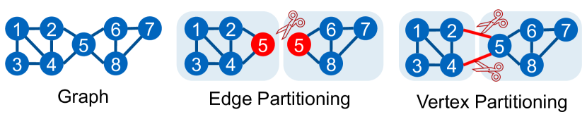
Figure 1. Edge partitioning vs. vertex partitioning.

Partitioner Types

Both edge and vertex partitioning algorithms can be categorized into (1) streaming partitioners, which stream the graph and directly assign vertices or edges to partitions (Xie et al., 2014; Petroni et al., 2015; Mayer et al., 2022; Mayer et al., 2018; Stanton and Kliot, 2012). Streaming partitioners can be further divided into stateless partitioners, which do not keep any state, and stateful streaming partitioners, which use some state, e.g., the current load per partition or to which partition vertices or edges were assigned. The state is considered for the assignments. (2) In-memory partitioners which load the complete graph into the memory (Karypis and Kumar, 1996; Martella et al., 2017; Zhang et al., 2017; Hanai et al., 2019; Sanders and Schulz, 2013). (3) Hybrid partitioners that partition one part with an in-memory partitioner and the remaining part with a streaming partitioner (Mayer and Jacobsen, 2021).

2.2. Graph Neural Network Training

Graph Neural Networks are a class of neural networks which operate on graph-structured data. GNNs iteratively learn on graphs by aggregating the local neighborhoods of vertices. At start, each vertex $v$ is represented by its feature vector $h^{(0)}_{v}$. In each layer, a vertex $v$ aggregates learned representations of its neighbors $N(v)$ of the previous layers, resulting in $a_{v}^{(k)}$ (Equation 1).

(1) $$a_{v}^{(k)}=\mathit{AGGREGATE}^{(k)}(\{h_{u}^{(k-1)}|u\in N(v)\})$$

A vertex updates its representation based on $a_{v}^{(k)}$ and its previous intermediate representation $h_{v}^{(k-1)}$ in layer $k-1$ by applying an update function (Equation 2).

(2) $$h_{v}^{(k)}=\mathit{UPDATE}^{(k)}(a_{v}^{(k)},h_{v}^{(k-1)})$$

The main approaches to train GNNs are full-batch and mini-batch training (Besta and Hoefler, 2022). In full-batch training, the entire graph is used to update the model once per epoch. In mini-batch training, each epoch contains multiple iterations, where a mini-batch is sampled from the graph and used for training and model update.

3. Experimental Methodology

Our study aims to investigate the effect of graph partitioning on the performance of distributed GNN training. We want to answer the following five research questions (RQ):

RQ-1:

How effective is graph partitioning for distributed GNN training in reducing training time and memory footprint?

RQ-2:

Do classical partitioning quality metrics accurately describe the effectiveness of partitioning algorithms for distributed GNN workloads? Which partitioning quality metric is most crucial?

RQ-3:

How much is the partitioning effectiveness influenced by GNN parameters such as the number of layers, hidden dimension, feature size, mini-batch size, and type of graph?

RQ-4:

What is the impact of the scale-out factor on the partitioning effectiveness?

RQ-5:

Can the invested partitioning time be amortized by a reduced GNN training time?

To answer these research questions, we conduct various experiments with two state-of-the-art distributed GNN systems: DistGNN (Md et al., 2021) and DistDGL (Zheng et al., 2020). DistDGL uses vertex partitioning and mini-batch training. DistGNN uses edge partitioning and full-batch training. This way, we cover a broad spectrum of GNN training modes. In the following, we introduce the datasets and metrics we use to evaluate both systems. Then, we describe the experiments for the respective system in more detail.

Datasets As known from distributed graph processing, different partitioning algorithms and graph processing workloads can be sensitive to the type of graph (Pacaci and Özsu, 2019; Verma et al., 2017). Therefore, we selected five graphs (see Table 1) from the following different categories (1) web, (2) social, (3) collaboration, (4) road, and (5) wiki. We randomly split the graphs into 10% training, 10% validation and 80% test vertices. Compared to large-scale distributed graph processing, all datasets only have a medium-sized graph structure. However, GNN workloads are much more communication, memory, and compute-intensive because the vertices have large feature vectors, and the computation includes heavy-weight neural network computations and leads to large intermediate states. Hence, graphs of this size already require heavy-weight processing for GNN training.

Table 1. Graphs of different types. Dir. indicates if the graph is directed or undirected. $|E|$ and $|V|$ are the number of edges and vertices, respectively.

Graph	Type	Dir.	$\mathbf{|E|}$	$\mathbf{|V|}$
Hollywood-2011 (HW) (Boldi and Vigna, 2004; Boldi et al., 2011)	Colla.	no	229M	2M
Dimacs9-USA (DI) (Kunegis, 2013)	Road	yes	58M	24M
Enwiki-2021 (EN) (Boldi and Vigna, 2004; Boldi et al., 2011)	Wiki	yes	150M	6M
Eu-2015-tpd (EU) (Boldi and Vigna, 2004; Boldi et al., 2011, 2014)	Web	yes	166M	7M
Orkut (OR) (Leskovec and Krevl, 2014)	Social	no	234M	3M

Table 2. Partitioning algorithms used in our evaluations.

Partitioner	Cut-Type	Category
Random	vertex-cut	Stateless streaming partitioning
DBH (Xie et al., 2014)	vertex-cut	Stateless streaming partitioning
HDRF (Petroni et al., 2015)	vertex-cut	Stateful streaming partitioning
2PS-L (Mayer et al., 2022)	vertex-cut	Stateful streaming partitioning
HEP10 (Mayer and Jacobsen, 2021)	vertex-cut	Hybrid partitioning
HEP100 (Mayer and Jacobsen, 2021)	vertex-cut	Hybrid partitioning
Random	edge-cut	Stateless streaming partitioning
LDG (Stanton and Kliot, 2012)	edge-cut	Stateful streaming partitioning
Spinner (Martella et al., 2017)	edge-cut	In-memory partitioning
Metis (Karypis and Kumar, 1996)	edge-cut	In-memory partitioning
ByteGNN (Zheng et al., 2022)	edge-cut	In-memory partitioning
KaHIP (Sanders and Schulz, 2013)	edge-cut	In-memory partitioning

Table 3. Different GNN hyper-parameters for both systems.

Hyper-parameter	Values
Hidden Dimension	16, 64, 512
Feature size	16, 64, 512
Number of layers	2, 3, 4

Infrastructure and infrastructure metrics For our experiments, we use a cluster composed of 32 machines. Each machine is equipped with 64GB memory and 8 CPU cores (Intel Core Haswell, 2.4 GHz, no TSX, IBRS). We measure the CPU and memory utilization and network traffic of each worker.

In the following Sections 4 and 5, we analyze the results for DistGNN and DistDGL, respectively.

4. DistGNN

4.1. Experiments

Graph partitioning algorithms We use six state-of-the-art edge partitioners from different categories (see. Table 2): (1) stateless streaming partitioning with random partitioning and DBH, (2) stateful streaming with HDRF and 2PS-L, and (3) hybrid-partitioning with HEP. HEP uses a parameter $\tau$ which influences how much of the graph is partitioned in a streaming fashion and how much in memory. A larger value for $\tau$ leads to a better partitioning quality as a larger part of the graph is partitioned in memory. As suggested by the authors, we set $\tau$ to 10 and 100 and treat these two configurations as two different partitioners HEP10 and HEP100 in our evaluations. HEP100 corresponds to in-memory partitioning, as the part not loaded into the memory is negligible if $\tau$ is set to $100$.

Workloads DistGNN currently only supports GraphSage (Hamilton et al., 2017), one of the most common model architectures (Zheng et al., 2020; Md et al., 2021; Hoang et al., 2021a; Su et al., 2021). We reviewed the GNN literature to identify commonly used hyper-parameters and chose the following to cover the ranges accordingly. We vary the hidden dimension from 16 to 512, the number of layers from 2 to 4, and the feature size from 16 to 512 (see Table 3).

Partitioning metrics We measure the well-known edge partitioning quality metrics replication factor, edge balance and vertex balance (see Section 2.1).

Training & partitioning time We measure the time per epoch. In addition, we measure the time spent in the forward pass, backward pass, synchronization of the model, and the optimizer step. Furthermore, we measure the partitioning time.

4.2. Partitioning Performance

We compare the partitioning algorithms regarding their communication costs and computational balance in the following.

Communication costs

We observe significant differences in terms of replication factors for the different partitioners. In all cases, HEP100 leads to the lowest (best) replication factor and Random to the largest (worst) one. Figure 2(b) shows, for example, that HEP100 at 32 partitions leads to a replication factor of $2.52$ on OR, which is much smaller compared to Random which leads to a replication factor of $22.2$. In general, more partitions lead to larger replication factors. For some partitioners, the replication factors increase more sharply than for others if the number of partitions increases.

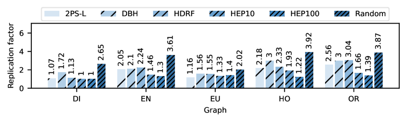
(a) 4 partitions.

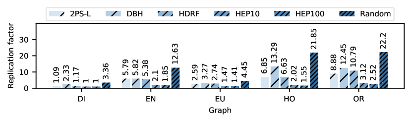
(b) 32 partitions.

Figure 2. Replication factors.

We observe a strong correlation ($R^{2}\geq 0.98$) between the replication factor and network traffic. This correlation is shown in Figure 3 for OR for different numbers of machines and number of layers and is also observed for the remaining graphs. The observation is plausible. The higher the replication factor, the more data is communicated via the network because more vertices are replicated and must synchronize their states.

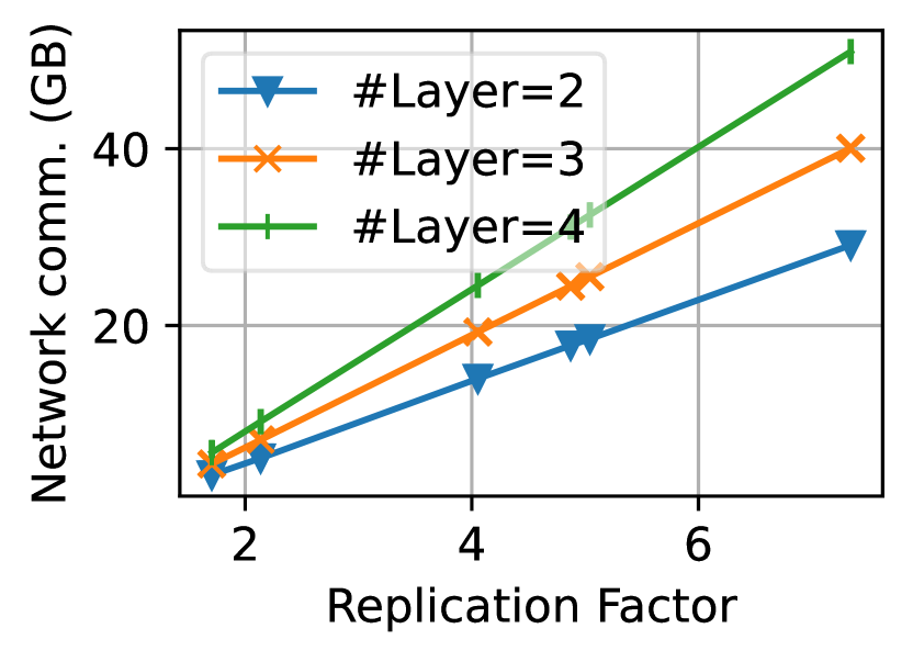
(a) 8 machines.

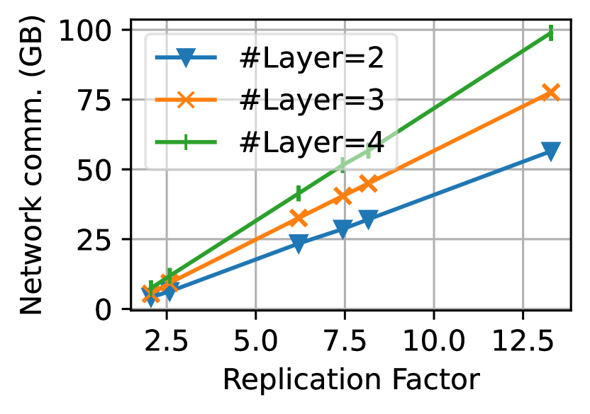
(b) 16 machines.

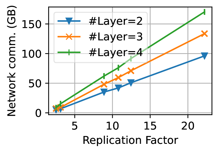
(c) 32 machines.

Figure 3. Replication factor vs. network communication for different number of machines and number of layers on OR.

We conclude that minimizing the replication factor is crucial for reducing network overhead.

Computational balance

It is crucial to balance the number of edges and vertices per partition. Each edge leads to an aggregation in the GNN, and neural network operations are performed for vertices. We observe a good edge balance of at most $\alpha\leq 1.11$ for all partitioners. However, we observe significant vertex imbalances (see Figure 4). Especially, the partitioners 2PS-L, HEP10 and HEP100 lead to large imbalances between $1.18$ and $1.89$ on 4 machines (see. Figure 4(a)) and can even increase up to 2.44 on 32 machines (see. Figure 4(b)). The vertex imbalance has a significant influence on the balance of memory utilization. Figure 5 reports the imbalance regarding memory utilization for all partitioners. We observe that vertex imbalance perfectly correlates with memory utilization imbalance.

We conclude that minimizing vertex imbalance is crucial for balancing memory utilization.

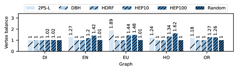
(a) 4 partitions.

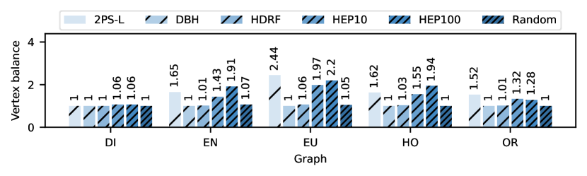
(b) 32 partitions.

Figure 4. Vertex balance.

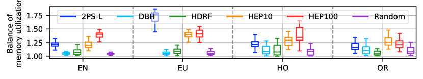
Figure 5. Memory utilization balance (4 machines).

Partitioning time

Figure 6 reports the partitioning time for partitioning all graphs into 4 and 32 partitions. We observe that the partitioning times of some algorithms, e.g., Random, 2PS-L and DBH, are less dependent on the number of partitions, compared to the remaining partitioners, where more partitions lead to higher partitioning times. For example, HDRF takes much more time to partition the graphs into 32 partitions compared to 4 partitions, which is expected because the complexity of the scoring function depends on the number of partitions.

In the following, we further analyze how the GNN training time is influenced by the partitioning metrics for different number of machines, and how GNN parameters influence the effectiveness of the partitioners.

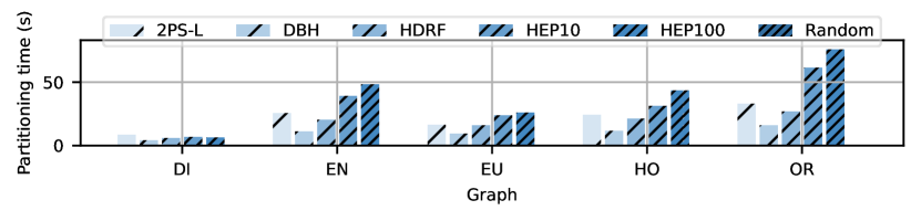
(a) 4 partitions.

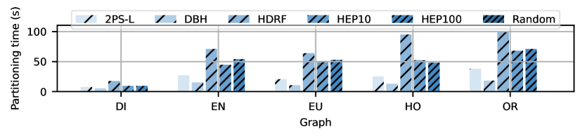
(b) 32 partitions.

Figure 6. Partitioning time.

4.3. GNN Training Performance

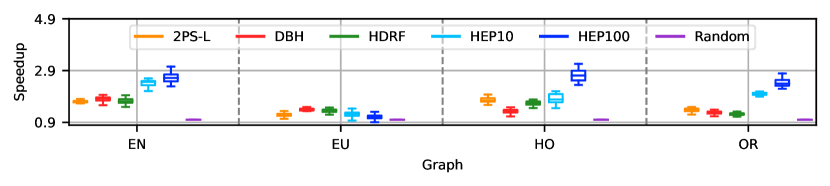
(a) 4 machines.

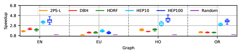
(b) 8 machines.

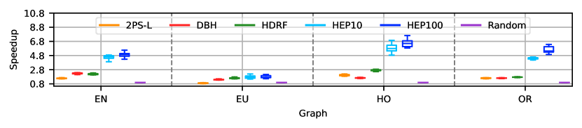
(c) 16 machines.

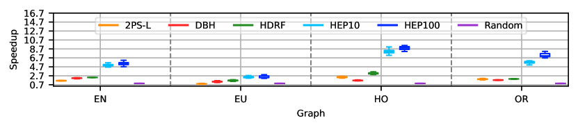
(d) 32 machines.

Figure 7. Speedup distribution of graph partitioners on 4, 8, 16 and 32 machines for all experiments.

In Figure 7, we report the speedup distribution for all partitioners compared to random partitioning for all combinations of feature size, hidden dimension and number of layers (see Table 3). We observe significant differences in terms of training time between the partitioners. HEP100 leads to the largest speedups of up to $3.53$, $6.18$, $8.15$ and $10.41$ on the graphs EU, EN, OR and HW, respectively. For example, on OR, compared to Random, on average DBH, 2PS-L, HDRF, HEP10 and HEP100 lead to speedups of $1.40$, $1.46$, $1.44$, $2.96$ and $3.68$ on 8 machines, $1.62$, $1.61$, $1.75$, $4.37$ and $7.16$ on 16 machines and $1.74$, $1.95$, $2.00$, $5.67$ and $7.16$ on 32 machines. We observe that the effectiveness in terms of speedup increases if the number of machines increases. Only 2PS-L on EU has a slowdown of 0.92, 0.92, and 0.91 on 8, 16 and 32 machines, respectively. We attribute this to the observation that the partitioning is highly imbalanced in terms of vertex balance, which we discuss in the following. We observe that a low replication factor is crucial to achieve large speedups. However, if the replication factor of two partitioners is close, it becomes clear that vertex balance is important as well. This can for example be seen in Figure 8. 2PS-L leads to a similar replication factor as HDRF and DBH on EN. However, 2PS-L leads to a large vertex imbalance while HDRF and DBH are perfectly balanced. We observe that 2PS-L leads to much smaller speedups which indicates that the vertex imbalance has a negative effect on the speedup.

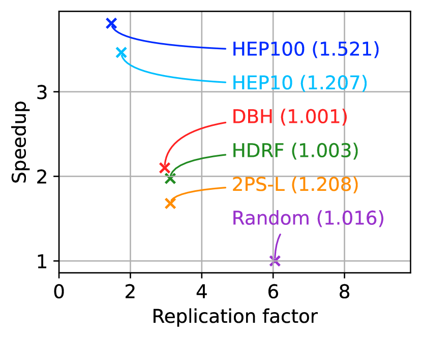
(a) 8 machines.

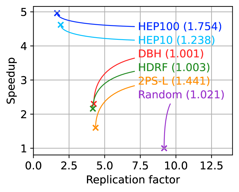
(b) 16 machines.

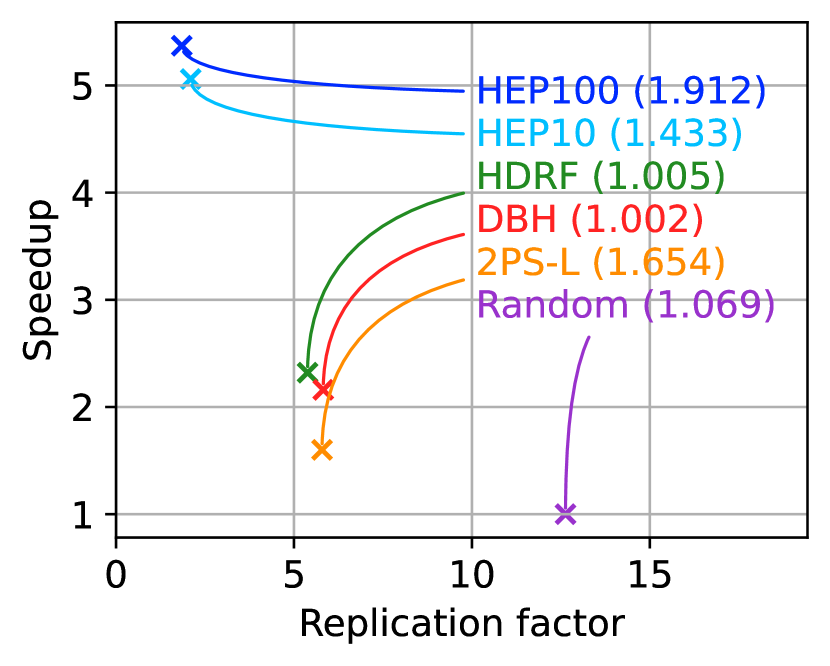
(c) 32 machines.

Figure 8. Replication factor vs. speedup on EN along with the vertex balance in the brackets.

In Figure 7, we observe only little spread in terms of speedup. In other words, the partitioners’ speedups are independent of the GNN parameters. We make a similar observation for network traffic. The savings are stable and not influenced much by the GNN parameters. This observation seems plausible. The replication factor influences for how many replicas the vertex state needs to be synchronized. The GNN parameters hidden dimension and feature size influence the state size and determine how much state needs to be synchronized. However, the ratio between the partitioners stays stable.

Figure 9(a) and Figure 9(b) give an overview of how much memory is needed for training with different partitioners in percent of random partitioning. We make two main observations. (1) The high-quality partitioners (HEP10 and HEP100) are much more effective than the other partitioners. (2) A large deviation indicates that the partitioners’ effectiveness depends on the GNN parameters. In the following, we first discuss why the partitioners differ in their effectiveness in terms of memory footprint and analyze how the GNN parameters influence this effectiveness.

We observe a strong correlation ($R^{2}\geq 0.99$) between the replication factor and memory footprint. Further, we observe that the memory footprint can heavily decrease, e.g., HEP100 reduces the memory for the graphs EU, OR, HW, EN by 37% 53%, 56% and 60% on 8 machines, by 44%, 60%, 65% and 63% on 16 machines and by 40%, 67%, 66% and 63% on 32 machines, respectively compared to Random. There are also cases where random partitioning leads to out-of-memory errors. For example, in all cases, DI can not be processed if random partitioning is applied, but in contrast, the more advanced partitioners enable the processing in many cases. In classical distributed graph processing, the replication factor is often minimized with the primary goal of reducing network communication. The memory load is less critical, especially if the vertex state is small which is the case for many graph processing algorithms such as BFS, DFS, Connected Components, PageRank, and K-cores. In contrast, in GNNs, the vertex state consists of large feature vectors meaning that the vertex state, not the graph structure, dominates the required memory. We conclude that minimizing the replication factor is crucial for minimizing the memory overhead and can be decisive for GNN training.

In the following, we analyze how the different GNN parameters influence the effectiveness of the partitioners in terms of memory.

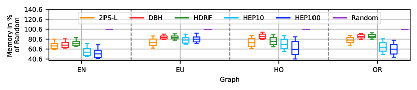
(a) 4 machines.

(b) 32 machines.

Figure 9. Distribution of memory footprint of graph partitioners in % of random partitioning on 4 and 32 machines.

(1) Feature size.

In Figure 10(a), we report the memory footprint for all partitioners in percent of random partitioning dependent on the feature size. We observe that if we keep all other parameters constant, an increase in the feature size increases the effectiveness. This result seems plausible. A fixed amount of memory is needed, e.g., for storing the graph structure. With an increasing feature size, the state to replicate increases, making partitioning more effective. We conclude, the larger the feature size, the higher the effectiveness of graph partitioners to reduce the memory footprint.

(2) Hidden dimension.

If the feature size and number of layers are kept constant, there will be some fixed amount of memory for the graph structure, the corresponding features, and the replication of the features. We observe that the higher the hidden dimension, the more effective the partitioners become (see Figure 10(b)). This observation seems reasonable. Larger hidden sizes lead to more state (intermediate representations) which needs to be synchronized among the machines as they are needed as the input of the next layer. We conclude that the larger the hidden dimension, the higher the effectiveness of graph partitioners to reduce the memory footprint.

(3) Number of layers.

The number of layers can influence the effectiveness of graph partitioning. The higher the number of layers, the more intermediate representations need to be stored (one per vertex and layer) which are needed in the backward pass. The replication factor influences to how many machines the intermediate representations are replicated, and the hidden dimension determines their size. We observe that, especially if the hidden dimension is large and the feature size is small, the effectiveness increases for more layers. This seems reasonable.

If the feature size is large and the hidden dimension is small, the effectiveness of graph partitioning remains relatively unaffected by the number of layers. This is because the state size is large due to the replication of large features. Increasing the number of layers results in more replications of small hidden representations, which does not significantly impact the memory footprint. However, if the feature size is small and the hidden dimension is large, increasing the number of layers leads to more replications of large hidden representations.

We conclude, the larger the hidden dimension and the smaller the features size, the higher the effectiveness of graph partitioners with an increasing number of layers increases.

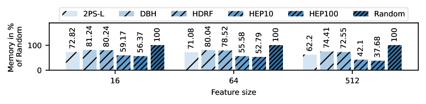
(a) Feature size.

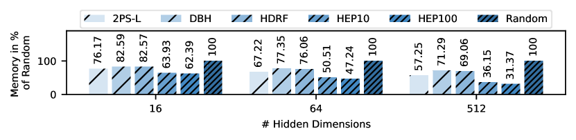
(b) Hidden dimensions.

Figure 10. Memory footprint in % of random partitioning dependant on different GNN hyper-parameters for OR on 8 machines.

(4) Scale-out factor.

In the following, we analyze how the scale-out factor influences the partitioners’ effectiveness in terms of speedup and memory footprint. Figure 11(a) shows the average speedup for all graph partitioners at different scale-out factors compared to random partitioning. We observe that the effectiveness of all graph partitioners increases if more machines are used for training. However, there are differences in how sharply the effectiveness increases. For the more light-weight partitioners 2PS-L, DBH and HDRF, the speedups increase moderately from 1.57, 1.37, and 1.49 on 4 machines to 1.79, 1.7, and 2.06 on 32 machines, respectively. The partitioners HEP10 and HEP100 lead to a speedup of 1.95 and 2.47 on 4 machines which increase sharply to 5.41 and 6.77 on 32 machines, respectively. We make similar observations for the memory overheads (see Figure 11(b)). All partitioners lead to substantial savings which increase if the number of machines increases. Both observations are plausible: In Figure 11(c), we report the achieved replication factors for all partitioners for all scale-out factors in percentages of Random, meaning lower numbers are better. We find that the replication factor of all partitioners increases less sharply than Random if the scale-out factor increases. We observe that the replication factors of 2PS-L, DBH, HDRF is 56.74%, 76.49% and 62.16% of Random on 4 machines and 39.99%, 60.81% and 48.58% of Random on 32 machines. HEP10 and HEP100 achieve a replication factor of 49.27% and 36.05% of Random on 4 machines and significant lower replication factors of 14.05% and 11.37% of Random on 32 machines, respectively.

We conclude that the effectiveness of graph partitioning is increasing both in terms of training time and memory overhead if the number of machines is increasing.

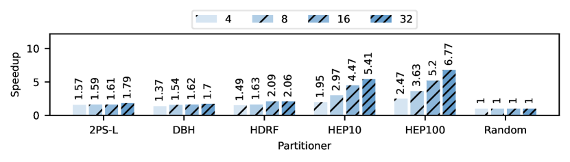
(a) Speedup (larger is better).

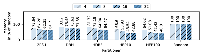
(b) Memory overhead (lower is better).

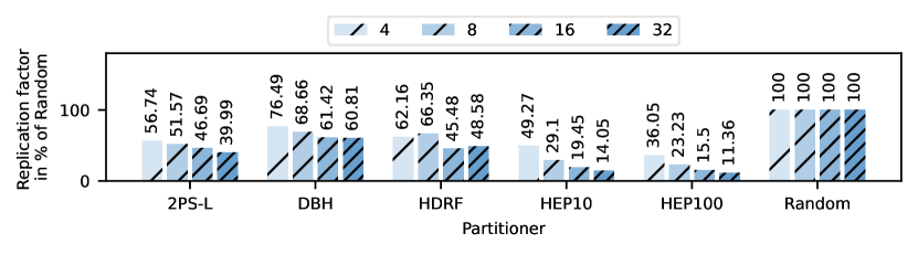
(c) Replication factor (lower is better).

Figure 11. The effectiveness of graph partitioning increases in terms of speedup and memory overhead if the scale-out factor is increased from 4 to 8, 16 and 32 machines.

(5) Partitioning time amortization

In Table 4, we report the average number of epochs until the partitioning time is amortized by faster training time for each combination of graph and partitioner. We assume that random partitioning does not take any time. DBH is the partitioner that amortizes the fastest: on average, it takes 1.39, 3.79, 3.05, and 3.83 epochs on the graphs EN, EU, HW and OR to amortize the partitioning time. HEP100 which leads to the largest speedups amortizes after 4.29, 12.0, 4.7, and 7.03 epochs on the graphs EN, EU, HW and OR. Full-batch training is often performed for hundreds of epochs (Md et al., 2021). Therefore, the partitioning time can be amortized. In addition, a hyper-parameter search is often performed which requires even more training epochs. Therefore, it is even more beneficial to invest in partitioning.

Table 4. Number of epochs until graph partitioning time is amortized by faster GNN training time. ”No” means no amortization is possible because of slowdown.

Graph	DBH	2PS-L	HDRF	HEP10	HEP100
EN	1.39	4.57	4.64	3.35	4.29
EU	3.79	no	8.8	10.15	12.0
HO	3.05	4.22	7.26	4.48	4.7
OR	3.83	7.39	11.69	6.64	7.03

5. DistDGL

5.1. Experiments

Graph partitioning algorithms We use six state-of-the-art vertex partitioners from different categories: (1) stateless streaming partitioning with random partitioning, (2) stateful streaming with LDG, and (3) in-memory partitioning with ByteGNN, Spinner, Metis, and KaHIP (see. Table 2).

Workloads We selected a representative set of graph neural network architectures commonly used in distributed GNN training, namely, GAT, GraphSage, and GCN. We use the same hyperparameters as for DistGNN (see Table 3). If not mentioned otherwise, we perform neighborhood sampling for all GNN models with the following configuration. Let $S_{i}$ be the number of neighbors to sample for layer $i$. For two layer GNNs, we use $l_{1}=25$ and $l_{2}=20$, for three layer GNNs $l_{1}=15$, $l_{2}=10$ and $l_{3}=5$ and for four layer GNNs, $l_{1}=10$, $l_{2}=10$, $l_{3}=5$ and $l_{4}=5$. We use a global batch size $GBS$ of 1024 if not stated otherwise. Therefore, each worker $w_{i}\in W$ trains with $\frac{GBS}{|W|}$ samples.

Partitioning metrics We compare the partitioners with the commonly used partitioning quality metrics edge-cut and vertex balance introduced in Section 2.1. In addition, we measure the training vertex balance. Further, we measure metrics based on the sampled mini-batches: the number of edges of the computation graphs, the number of local input vertices, and the number of vertices that need to be fetched via the network.

Training & Partitioning Time We measure the epoch and step time and all phases (mini-batch sampling, feature loading, forward pass, backward pass, and model update) for each step. In addition, we measure the partitioning time.

5.2. Partitioning Performance

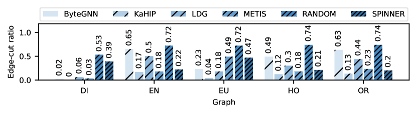
(a) 4 partitions.

(b) 32 partitions.

Figure 12. Edge-cut ratio for all combinations of graph, number of partitions and graph partitioner.

In the following, we compare the graph partitioners regarding communication costs and computational balance.

Communication Costs

In Figure 12, we report the achieved edge-cut ratio for each combination of graph, graph partitioning algorithm, and number of partitions. In most cases, KaHIP achieves the lowest edge-cut and random partitioning leads to the largest edge-cut. We observe significant differences between the partitioning algorithms in terms of edge-cut, e.g., KaHIP achieves an edge-cut ratio smaller than 0.001 and 0.12 on the graph DI and EU for 32 partitions, respectively, which is much lower (better) compared to random partitioning which leads to edge-cuts of 0.68 and 0.93 for the same graphs. We also observed for all partitioning algorithms that a higher number of partitions leads to a larger edge-cut.

In the following, we investigate the influence of the edge-cut on network communication. There are cases where a lower edge-cut results in less network communication. However, there are also cases where even if the edge-cut of different partitioners is similar, the network communication can differ a lot. For example, we observed that Spinner has an edge-cut lower than Metis on OR, but the network communication is much higher.

This observation seems reasonable. There can be edges that are more frequently involved in the sampling process. If these edges are cut, they lead to more network traffic than edges hardly visited in the sampling process. To ensure that the observed anomaly is related to graph partitioning, we measure for each mini-batch the number of vertices needed for processing the mini-batch that are not local to the respective worker. We define these vertices as remote vertices. We observe a strong correlation between the number of remote vertices and network traffic. We conclude that edge-cut is not always a perfect predictor for network traffic and that there are cases where a lower edge-cut still leads to more remote vertices and higher network traffic.

Computation Balance

For efficient distributed graph processing, it is crucial that the computation is balanced among machines which is measured via the vertex balance. However, unlike distributed graph processing algorithms such as PageRank, the computational load of mini-batch GNN training depends on the size of the sampled mini-batches. Each worker samples a mini-batch based on the k-hop neighborhood of the training vertices. To ensure load balance, it is essential that the computation graphs of mini-batches are of similar size. We define the number of vertices that are needed to compute a mini-batch as the input vertices and input vertex balance per step as the number of input vertices of the largest mini-batch divided by the average number of input vertices per mini-batch in the respective step. In Figures 14(a)-14(b), we report the imbalance of the mini-batches in terms of input vertices. We observe a large imbalance, which is increasing as the number of partitions is increased.

Figure 13. Training vertex balance (8 partitions).

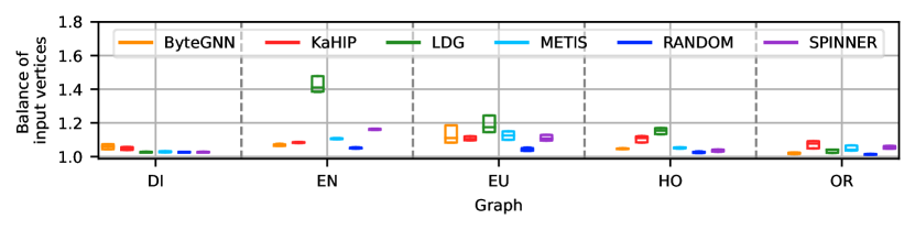
(a) 4 machines.

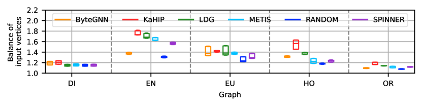
(b) 32 machines.

Figure 14. Balance in terms of input vertices of the mini-batches for the GraphSage model.

Partitioning Time

In Figure 15, we report the partitioning time for all graphs and partitioning algorithms for 4 and 32 partitions. We observe that the best (in terms of lowest edge-cut) performing partitioner KaHIP, leads to the highest partitioning time.

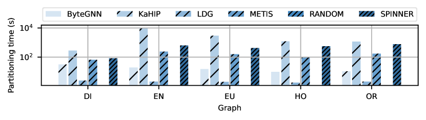
(a) 4 partitions.

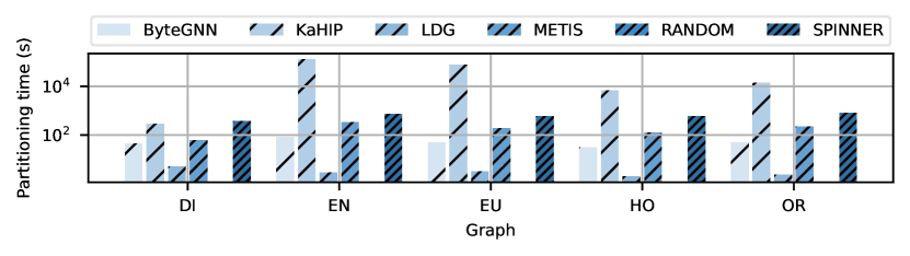
(b) 32 partitions.

Figure 15. Partitioning time on a logarithmic scale.

In the following, we investigate the influence of the partitioning metrics on the actual GNN training time and analyze how the GNN hyper-parameters influence the effectiveness of the graph partitioners.

5.3. GNN Training Performance

In Figure 16, we report the average speedups for all combinations of feature size, hidden dimension and number of layers (see Table 3) for all graph partitioners with random partitioning as a baseline on 4, 8, 16 and 32 machines for the GraphSage architecture. In our experiments, KaHIP and Metis lead to the largest speedups of up to 1.84, 1.84, 3.09 and 3.47 on a cluster with 4, 8, 16 and 32 machines, respectively. Therefore, graph partitioning is an important preprocessing step for distributed GNN training.

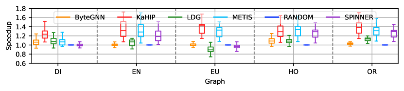
(a) 4 machines.

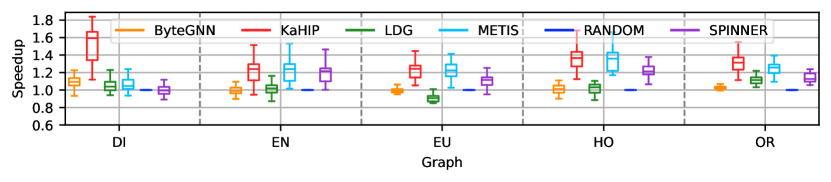
(b) 8 machines.

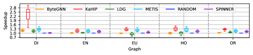
(c) 16 machines.

(d) 32 machines.

Figure 16. Speedup distribution of graph partitioners on 4, 8, 16 and 32 machines for all GraphSage experiments.

In Figure 16, we see significant variances in terms of speed up that indicate that the effectiveness of the partitioning algorithms depends on the GNN parameters. Therefore, we conduct a detailed analysis of how different GNN parameters influence the different training phases and how the partitioners differ from each other. On each worker in each step, we measure the phase times (1) mini-batch sampling, (2) feature loading, (3) forward pass, (4) backward pass, and (5) model update. In each step, we identify the worker which leads to the longest mini-batch sampling, feature loading and forward pass time as the straggler. We exclude the time for the backward pass because it also contains the time for the all-reduce operation in which the gradients are synchronized between the workers. The model update time is negligible. Then, we get the phase times of the slowest worker per step and sum up the phase times of all steps of the respective slowest worker. In other words, we are interested in how much time the straggler spends on average in each phase. In the following, we investigate how the different GNN model parameters influence the effectiveness of graph partitioning in terms of speedup of the distributed training compared to random partitioning. In Figure 17, we observe large imbalances for all partitioners, showing that even if the number of training vertices is balanced, the computation time can be imbalanced. Interestingly, all partitioners lead to large imbalances.

(a) 4 machines.

(b) 32 machines.

Figure 17. Balance in terms of training time.

(1) Feature size

We observe that the effectiveness of partitioning increases with larger feature sizes. Figures 18(a)-18(b) shows the speedup for the partitioners compared to random partitioning dependent on the feature size. For example, in Figure 18(a), the training for GraphSage with KaHIP leads to a speedup of 1.23 and 1.52 for a feature size of 16 and 512, respectively. This observation is plausible. As feature sizes increase, network communication increases because larger feature vectors are sent over the network, making graph partitioning even more valuable in reducing communication costs.

(a) Increasing feature size (4 machines).

(b) Increasing feature size (32 machines).

Figure 18. Speedup of graph partitioners for the GraphSage model on 4 and 32 machines for different feature sizes.

Detailed: For each combination of number layers and hidden dimension, we vary the feature size. We make the following key observations: (1) The larger the feature size, the longer the feature fetching phase (see Figure 19(a)) while the sampling time stays constant. We also observe that for small feature sizes (up to 64), the sampling takes more time than fetching features, but for large feature sizes of 512, the time for feature fetching dominates the sampling time by a lot (see Figure 19(a)). In contrast, for the road network DI, we observe that sampling always takes more time than fetching features (see Figure 19(b)) which seems plausible because the mean degree in the road network is small and the skew of the degree distribution is low. Therefore, the sampled mini-batches are small, and only a few input vertices must be fetched. We also observe that the edge-cut for the road network is much lower than for the remaining graphs (see Figure 12). (2) The forward and backward pass time increases with larger feature sizes, which is plausible because more computations will be performed in the first layer.

We observe that the partitioners differ a lot from each other when varying the feature size and that the feature size influences the different phases. The feature fetching phase is influenced most, which can for example be seen in Figure 19(a) for training a three layer GraphSage with a hidden dimension of 64 on the graph EU. In most cases, the better the partitioner in terms of edge-cut, the lower the communication costs, which can speed up both the mini-batch sampling and the feature fetching phase.

(a) Graph: EU.

(b) Graph: DI.

Figure 19. Phase times for a 3 layer GraphSAGE model with a hidden dimension of 64 on 4 machines for different feature sizes.

(2) Number of hidden dimensions

We found that partitioning becomes less crucial as the hidden dimension increases. For example, compared with random partitioning, KaHIP leads to a speedup of 1.38 and 1.19 and Metis 1.31 and 1.15 for a hidden dimension of 16 and 512, respectively. This result is reasonable since an increased hidden size leads to greater computational costs, potentially dominating the communication costs.

Detailed: We vary the hidden dimension for each combination of feature size and number of layers. Our main observations are: (1) sampling and feature loading time stay constant, which is expected as only the neural network operations are influenced by the hidden dimension. The larger the hidden dimension, the more time is used for computation. (2) We also observe that the effectiveness of partitioners decreases for the larger hidden sizes because most of the differences are in feature loading and sampling. However, if the hidden size increases, the computation takes a larger share of the overall training time. Therefore, the difference between the partitioners is lower.

(a) Increasing hidden dimensions (4 machines).

(b) Increasing hidden dimensions (32 machines).

Figure 20. Speedup of graph partitioners for the GraphSage model on 4 and 32 machines for different hidden dimensions.

Figure 21. Times of different phases for a GraphSAGE model with a hidden dimension and feature size of 64 on 4 machines for the OR graph.

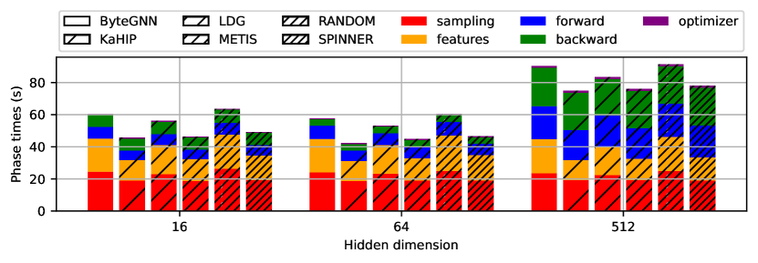
Figure 22. Times of different phases for a 3 layer GraphSAGE with a feature size of 64 on 4 machines for the OR graph.

(3) Number of Layers

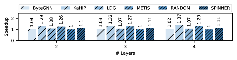
(a) Increasing the number of layers (4 machines).

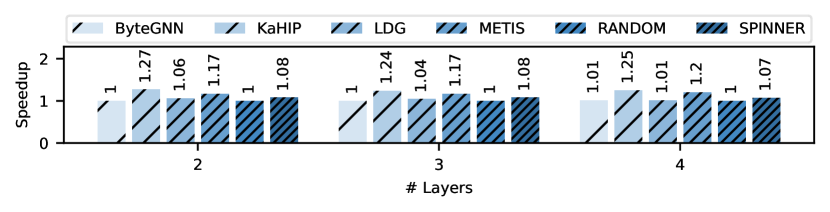
(b) Increasing the number of layers (32 machines).

Figure 23. Speedup of graph partitioners for the GraphSage model on 4 and 32 machines for different number of layers.

We observe that the effectiveness of the partitioners remains relatively unaffected by an increasing number of layers. In some cases, the effectiveness slightly increases or decreases, but the influence is much smaller than the influence of the feature size and hidden dimension, and there is also no clear trend. This is an unexpected observation. One could think that the effectiveness of the partitioning algorithms would heavily decrease if the number of layers increases because large parts of the graph will be contained in the mini-batches, but still, the partitioning algorithms lead to different training times, and many partitioners outperform random partitioning.
Detailed: We vary the number of layers for each combination of feature size and hidden dimension. We make the following key observations: (1) All phases increase in run-time if the number of layers increases. This is expected because an increase in the number of layers leads to larger computation graphs within the mini-batches, which increase the communication costs (more remote accesses in the sampling phase and more remote vertices to fetch via the network) and the computation costs (more neural network operations). (2) We observe, especially for 3 and 4 layer GraphSage, that most of the speedup gained by different partitioning algorithms comes from faster sampling and feature fetching (see Figure 21).

(4) Scale-out factor

In the following, we investigate the effectiveness of scaling out distributed GNN training to more machines for all partitioning algorithms. We scale out from 4 to 8, 16 and 32 machines. We make the following observations: (1) For DI, scaling out increases the effectiveness of the partitioners. Especially for the partitioners KaHIP, Metis, LDG and ByteGNN, the effectiveness increases a lot. However, for Spinner, the effectiveness stays relatively constant. This seems plausible as the edge-cut for Random and Spinner is far higher on DI than for the remaining partitioners (see Figure 12). (2) For the remaining graphs, we observe that the effectiveness of GraphSage decreases on average (see Figure 24(a)). For example, KaHIP and Metis lead to a speedup of 1.32 and 1.27 on 4 machines and to a smaller speedup of 1.25 and 1.19 on 32 machines, respectively. We found that the number of remote vertices (see Figure 24(b)) and the edge-cut (see Figure 24(c)) of the partitioners in percentages of Random is increasing when scaling out to more machines. We also observe that the network communication of the partitioners in percentages of Random is also increasing. In other words, the effectiveness of the partitioners is also decreasing in terms of partitioning metrics and network communication compared to Random, when the number of machines increases. It is worth to note that the feature loading phase scales really well. We found that large feature sizes make partitioning more effective. For large feature vectors and few machines, the feature fetching phase can take a large share of the training time and also leads to large differences between the partitioners (see Figures 25(a) and 25(b)). The feature fetching phase can decrease sharply when scaling out to more machines. Therefore, the difference between the partitioners is decreasing, resulting in lower effectiveness. We make a similar observation with the sampling phase. We conclude that in most cases, the effectiveness of partitioning slightly decreases if the scale-out factor increases.

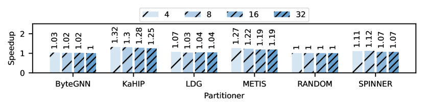
(a) Speedup

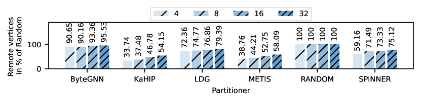
(b) Remote vertices.

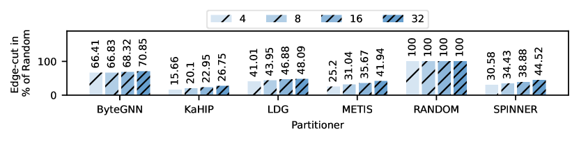
(c) Edge-cut

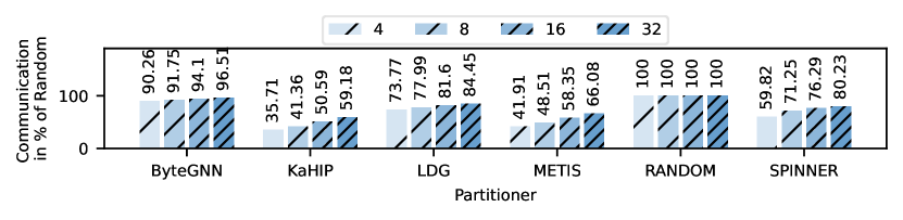
(d) Communication.

Figure 24. The effectiveness of partitioning decreases when scaling GraphSage from 4 to 32 machines.

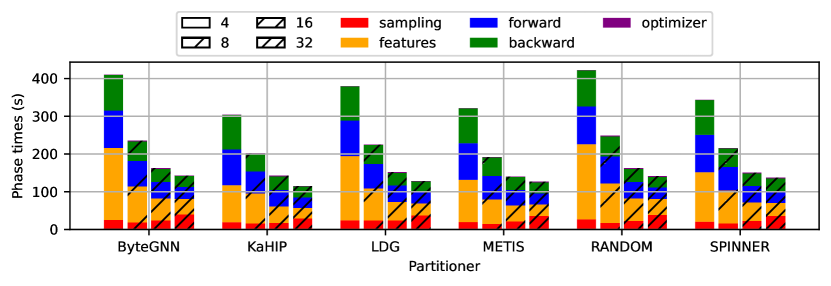
(a) GAT

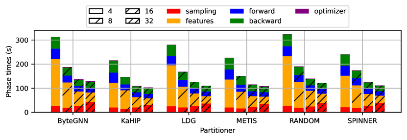
(b) GraphSage.

Figure 25. Phase times for a 3 layer GAT and GraphSage with a feature size of 512 and a hidden dimension of 64 on the OR graph trained with 4, 8, 16 and 32 machines.

(5) Partitioning time amortization

In Table 5, we report the average number of epochs until the partitioning time is amortized by faster training time for each combination of graph and partitioner. We observe that the partitioning time can be amortized by faster GNN training. However, KaHIP, the partitioner which leads to the largest speedups only amortizes for DI but not for the remaining graphs. However, Metis, which also leads to significant speedups, does amortize for all graphs.

Table 5. Number of epochs until graph partitioning time is amortized by faster GNN training time. ”No” means no amortization is possible because of slowdown.

Graph	ByteGNN	KaHIP	LDG	SPINNER	METIS
DI	0.93	2.61	0.1	14.37	1.13
EN	2.16	2501.93	0.39	54.07	16.79
EU	no	1197.25	no	53.8	8.14
HO	0.68	347.51	0.47	77.78	10.7
OR	3.14	223.19	0.27	70.19	14.59

5.4. Influence of mini-batch size on partitioner effectiveness

The following experiments aim to investigate the influence of the mini-batch size on the effectiveness of partitioning. In other words, we want to evaluate if the partitioning is more crucial (in terms of reduced training time) if the mini-batch size increases.

We fix the number of workers to 16 and set the mini-batch size to 512, 1024, 2048, 4096, 8192, 16384, and 32768 for a three layer GAT and a three layer GraphSage. For both GNN architectures, we use two configurations: (1) hidden dimension and feature size of 64 (low communication) and (2) hidden dimension of 64 and feature size of 512 (high communication).

We observe for all partitioners that the network traffic decreases if the batch size increases compared to Random (see Figure 26(b)). For example, KaHIP and Spinner lead to a network communication of 66% and 77% of Random with a batch size of 512 and of 48% and 67% if the batch size is set to 32768, respectively. We observe a similar trend for the number of remote vertices (see Figure 26(c)). This seems reasonable. Many vertices can end up in different mini-batches. However, if the mini-batch increases, the overlap in the larger mini-batches increases, leading to fewer remote vertices.

The effectiveness of the partitioners can decrease or increase with larger batch sizes if the feature size is 64: However, there is no clear trend. In contrast, if the features size is 512, in most cases, the effectiveness of the partitioners increases for ByteGNN, KaHIP, Metis and Spinner on the graphs HW, EU, EN and OR. For example, Figure 26(a) shows that training with KaHIP and Metis lead to a speed up of 1.27 and 1.13 for a small batch size of 512 and to a larger speed up of 1.91 and 1.65 if the batch size is set to 32768. We conclude that larger batch sizes increase the partitioner effectiveness for large feature sizes.

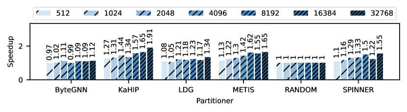
(a) Speedup compared to Random.

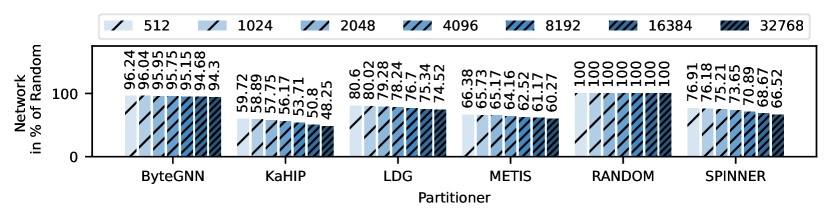
(b) Network communication in % of Random.

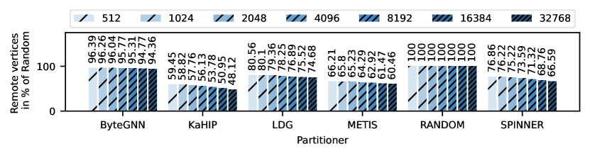
(c) Number of remote vertices in % of Random.

Figure 26. Different metrics for a 3 layer GraphSage with a hidden dimension of 64 and feature size of 512 on the OR graph for varying batch sizes between 512 and 32768.

6. Lessons learned

In the following, we summarize our main findings and refer them to the research questions introduced in Section 3.

(1) Graph partitioning is effective to speed up GNN training (RQ-1). We observed large speedups of up to 10.41 and 3.4 for DistGNN and DistDGL, respectively. The speedups achieved for DistDGL are comparable to those seen in distributed graph processing (Mayer and Jacobsen, 2021; Merkel et al., 2023; Mayer et al., 2022). However, the speedups for DistGNN are higher. Full-batch training leads to large communication and memory overheads, both heavily influenced by graph partitioning, which makes graph partitioning crucial for efficient distributed full-batch GNN training.

(2) Graph partitioning is effective in reducing the memory footprint (RQ-1). We found that the replication factor perfectly correlates with the amount of necessary memory. Different from classical distributed graph processing, where the state of vertices is small, in GNNs, the state of vertices is large. The vertices can have large feature vectors and intermediate representations that must be stored for all vertices. Minimizing the replication factor leads to significant memory savings because fewer vertex states are replicated. We observe many cases where advanced partitioning algorithms leading to small replication factors can reduce the necessary amount of memory by up to 85.1%. Therefore, the replication factor determines whether training a GNN with the given memory budget is possible at all.

(3) Classical partitioning metrics are relevant for GNN performance (RQ-2). For both DistDGL and DistGNN, we observed that both communication and balancing metrics are important. Especially for DistGNN, we observed that the replication factor has a large correlation with the network communication, the memory overhead, and ultimately the training time. Minimizing the replication factor to reduce the GNN training time is crucial. We also found that in cases where two different partitioners lead to a similar replication factor, balancing the vertices becomes important. Furthermore, vertex balance perfectly correlates with memory utilization balance which is crucial fur memory-intensive full-batch training. This is an important insight, as most edge partitioners balance the number of edges per partition and do not focus on balancing vertices.

(4) GNN parameters influence the effectiveness of graph partitioners (RQ-3). Unlike distributed graph processing, in GNN training, the GNN models have parameters, such as the number of layers, the hidden dimension, or the batch size, and the graphs have attached features. For DistDGL, we observed that GNN parameters influence the partitioners’ effectiveness. Graph partitioning is effective, especially if the feature vectors are large and the hidden dimensions are low. We also found that if the feature size is large and the mini-batch size increases, the effectiveness increases a lot. For DistGNN, we observe that effectiveness in terms of training run-time is less dependent on the GNN parameters. However, regarding memory overhead, the effectiveness increases if the feature size, the hidden dimension or the number of layers increases.

(5) The scale-out factor influences the effectiveness of graph partitioners (RQ-4). For DistDGL, we observe that in most cases, the effectiveness of graph partitioning slightly decreases when scaling out to more machines. However, for DistGNN, graph partitioning becomes very important because the network costs increase significantly.

(6) Partitioning can be amortized by faster GNN training (RQ-5). For both DistDGL and DistGNN, we found that the invested graph partitioning time can in many cases be amortized already after a few epochs, making graph partitioning an important optimization for distributed GNN training.

7. Related Work

Different studies (Verma et al., 2017; Abbas et al., 2018; Gill et al., 2018; Pacaci and Özsu, 2019) have been conducted to investigate how graph partitioning influences the performance of distributed graphs processing systems. Verma et al. (Verma et al., 2017) study the graph partitioning algorithms available in GraphX (Gonzalez et al., 2014), PowerGraph (Gonzalez et al., 2012), and PowerLyra (Chen et al., 2015) for graph analytics. Abbas et al. (Abbas et al., 2018) study streaming graph partitioners and compare them in a graph processing framework based on Apache Flink (Carbone et al., 2015) for graph analytics. Gill et al. (Gill et al., 2018) investigate the influence of different partitioning strategies in D-Galois for graph analytics workloads. Pacaci and Özsu (Pacaci and Özsu, 2019) study streaming graph partitioning algorithms for graph analytics with PowerLyra and online graph query workloads with JanusGraph (jan, 2023). The studies focus on classical graph workloads. However, distributed GNN training is different. First, GNN training leads to large memory and communication overheads. Huge feature vectors and large intermediate states are computed, stored, and sent over the network. Second, the computations consist of computationally expensive neural network operations. Third, the GNN workloads are not only characterized by the model architecture, but also by GNN parameters such as the number of layers and hidden dimension. Forth, mini-batch-based training has a complex data loading phase which consists of distributed multi-hop sampling followed by a communication intensive feature loading phase.

Graph partitioning is a vibrant research area and many different approaches exist (Sanders and Schulz, 2013; Mayer et al., 2018; Mayer et al., 2022; Mayer and Jacobsen, 2021; Xie et al., 2014; Petroni et al., 2015; Zhang et al., 2017; Hanai et al., 2019; Margo and Seltzer, 2015; Karypis and Kumar, 1996; Patwary et al., 2019; Nishimura and Ugander, 2013; Schlag et al., 2019; Stanton and Kliot, 2012; Martella et al., 2017; Slota et al., 2017; Pellegrini and Roman, 1996; Zwolak et al., 2022; Hoang et al., 2021b; Merkel et al., 2023). See (Çatalyürek et al., 2023) for a recent survey about graph partitioning. We selected a representative set of different categories.

Many distributed graph neural network systems exist (Md et al., 2021; Zheng et al., 2020; Thorpe et al., 2021; Zheng et al., 2022; Su et al., 2021; Hoang et al., 2021a; Gandhi and Iyer, 2021). A recent survey (Vatter et al., 2023) gives an overview of different systems and compares those along different axis, also graph partitioning. We extend this research by experimentally investigating the effectiveness of graph partitioning for GNN training.

8. Conclusions

In our work, we performed an experimental evaluation to investigate the effectiveness of graph partitioning for distributed GNN training. We showed that graph partitioning is an essential optimization for distributed GNN training and that different factors such as GNN parameters (e.g., hidden dimension, number of layers, mini-batch size, etc.), the scale-out factor, and the feature size can influence the effectiveness of graph partitioning for GNN training, both in terms of memory footprint and training time. Further, we found that invested partitioning time can be amortized by reduced GNN training time. Based on our findings, we conclude that graph partitioning has great potential to make GNN training more effective. We hope our research can spawn the development of even more effective graph partitioning algorithms in the future.

References

- (1)
- jan (2023) 2023. JanusGraph. Accessed: 19 July 2023, https://janusgraph.org/.
- Abbas et al. (2018) Zainab Abbas, Vasiliki Kalavri, Paris Carbone, and Vladimir Vlassov. 2018. Streaming Graph Partitioning: An Experimental Study. Proc. VLDB Endow. 11, 11 (July 2018), 14. https://doi.org/10.14778/3236187.3236208
- Besta and Hoefler (2022) Maciej Besta and Torsten Hoefler. 2022. Parallel and distributed graph neural networks: An in-depth concurrency analysis. arXiv preprint arXiv:2205.09702 (2022).
- Boldi et al. (2014) Paolo Boldi, Andrea Marino, Massimo Santini, and Sebastiano Vigna. 2014. BUbiNG: Massive Crawling for the Masses. In Proceedings of the Companion Publication of the 23rd International Conference on World Wide Web. International World Wide Web Conferences Steering Committee, 227–228.
- Boldi et al. (2011) Paolo Boldi, Marco Rosa, Massimo Santini, and Sebastiano Vigna. 2011. Layered Label Propagation: A MultiResolution Coordinate-Free Ordering for Compressing Social Networks. In Proceedings of the 20th international conference on World Wide Web, Sadagopan Srinivasan, Krithi Ramamritham, Arun Kumar, M. P. Ravindra, Elisa Bertino, and Ravi Kumar (Eds.). ACM Press, 587–596.
- Boldi and Vigna (2004) Paolo Boldi and Sebastiano Vigna. 2004. The WebGraph Framework I: Compression Techniques. In Proc. of the Thirteenth International World Wide Web Conference (WWW 2004). ACM Press, Manhattan, USA, 595–601.
- Carbone et al. (2015) Paris Carbone, Asterios Katsifodimos, Stephan Ewen, Volker Markl, Seif Haridi, and Kostas Tzoumas. 2015. Apache flink: Stream and batch processing in a single engine. Bulletin of the IEEE Computer Society Technical Committee on Data Engineering 36, 4 (2015).
- Çatalyürek et al. (2023) Ümit Çatalyürek, Karen Devine, Marcelo Faraj, Lars Gottesbüren, Tobias Heuer, Henning Meyerhenke, Peter Sanders, Sebastian Schlag, Christian Schulz, Daniel Seemaier, and Dorothea Wagner. 2023. More Recent Advances in (Hyper)Graph Partitioning. ACM Comput. Surv. 55, 12, Article 253 (mar 2023), 38 pages. https://doi.org/10.1145/3571808
- Chen et al. (2015) Rong Chen, Jiaxin Shi, Yanzhe Chen, and Haibo Chen. 2015. PowerLyra: Differentiated Graph Computation and Partitioning on Skewed Graphs. In Proceedings of the Tenth European Conference on Computer Systems (Bordeaux, France) (EuroSys ’15). Association for Computing Machinery, New York, NY, USA, Article 1, 15 pages. https://doi.org/10.1145/2741948.2741970
- Fan et al. (2019) Wenqi Fan, Yao Ma, Qing Li, Yuan He, Eric Zhao, Jiliang Tang, and Dawei Yin. 2019. Graph Neural Networks for Social Recommendation. In The World Wide Web Conference (San Francisco, CA, USA) (WWW ’19). Association for Computing Machinery, New York, NY, USA, 417–426. https://doi.org/10.1145/3308558.3313488
- Gandhi and Iyer (2021) Swapnil Gandhi and Anand Padmanabha Iyer. 2021. P3: Distributed Deep Graph Learning at Scale. In 15th USENIX Symposium on Operating Systems Design and Implementation (OSDI 21). USENIX Association, 551–568. https://www.usenix.org/conference/osdi21/presentation/gandhi
- Gill et al. (2018) Gurbinder Gill, Roshan Dathathri, Loc Hoang, and Keshav Pingali. 2018. A Study of Partitioning Policies for Graph Analytics on Large-Scale Distributed Platforms. Proc. VLDB Endow. 12, 4 (Dec. 2018), 14. https://doi.org/10.14778/3297753.3297754
- Gonzalez et al. (2012) Joseph E. Gonzalez, Yucheng Low, Haijie Gu, Danny Bickson, and Carlos Guestrin. 2012. PowerGraph: Distributed Graph-Parallel Computation on Natural Graphs. In Proceedings of the 10th USENIX Conference on Operating Systems Design and Implementation (Hollywood, CA, USA) (OSDI’12). USENIX Association, USA, 14.
- Gonzalez et al. (2014) Joseph E. Gonzalez, Reynold S. Xin, Ankur Dave, Daniel Crankshaw, Michael J. Franklin, and Ion Stoica. 2014. GraphX: Graph Processing in a Distributed Dataflow Framework. In Proceedings of the 11th USENIX Conference on Operating Systems Design and Implementation (Broomfield, CO) (OSDI’14). USENIX Association, USA, 15.
- Hamilton et al. (2017) Will Hamilton, Zhitao Ying, and Jure Leskovec. 2017. Inductive representation learning on large graphs. Advances in neural information processing systems 30 (2017).
- Hanai et al. (2019) Masatoshi Hanai, Toyotaro Suzumura, Wen Jun Tan, Elvis Liu, Georgios Theodoropoulos, and Wentong Cai. 2019. Distributed Edge Partitioning for Trillion-Edge Graphs. Proc. VLDB Endow. 12, 13 (Sept. 2019), 14. https://doi.org/10.14778/3358701.3358706
- Hoang et al. (2021a) Loc Hoang, Xuhao Chen, Hochan Lee, Roshan Dathathri, Gurbinder Gill, and Keshav Pingali. 2021a. Efficient distribution for deep learning on large graphs. update 1050 (2021), 1.
- Hoang et al. (2021b) Loc Hoang, Roshan Dathathri, Gurbinder Gill, and Keshav Pingali. 2021b. CuSP: A Customizable Streaming Edge Partitioner for Distributed Graph Analytics. SIGOPS Oper. Syst. Rev. 55, 1 (jun 2021), 47–60. https://doi.org/10.1145/3469379.3469385
- Karypis and Kumar (1996) George Karypis and Vipin Kumar. 1996. Parallel Multilevel K-Way Partitioning Scheme for Irregular Graphs. In Proceedings of the 1996 ACM/IEEE Conference on Supercomputing (Pittsburgh, Pennsylvania, USA) (Supercomputing ’96). IEEE Computer Society, USA. https://doi.org/10.1145/369028.369103
- Kunegis (2013) Jérôme Kunegis. 2013. KONECT: The Koblenz Network Collection. In Proceedings of the 22nd International Conference on World Wide Web (Rio de Janeiro, Brazil) (WWW ’13 Companion). Association for Computing Machinery, New York, NY, USA, 1343–1350. https://doi.org/10.1145/2487788.2488173
- LeClair et al. (2020) Alexander LeClair, Sakib Haque, Lingfei Wu, and Collin McMillan. 2020. Improved Code Summarization via a Graph Neural Network. In Proceedings of the 28th International Conference on Program Comprehension (Seoul, Republic of Korea) (ICPC ’20). Association for Computing Machinery, New York, NY, USA, 184–195. https://doi.org/10.1145/3387904.3389268
- Leskovec and Krevl (2014) Jure Leskovec and Andrej Krevl. 2014. SNAP Datasets: Stanford Large Network Dataset Collection. http://snap.stanford.edu/data.
- Li et al. (2021) Shuangli Li, Jingbo Zhou, Tong Xu, Liang Huang, Fan Wang, Haoyi Xiong, Weili Huang, Dejing Dou, and Hui Xiong. 2021. Structure-Aware Interactive Graph Neural Networks for the Prediction of Protein-Ligand Binding Affinity. In Proceedings of the 27th ACM SIGKDD Conference on Knowledge Discovery & Data Mining (Virtual Event, Singapore) (KDD ’21). Association for Computing Machinery, New York, NY, USA, 975–985. https://doi.org/10.1145/3447548.3467311
- Liu et al. (2021) Yang Liu, Xiang Ao, Zidi Qin, Jianfeng Chi, Jinghua Feng, Hao Yang, and Qing He. 2021. Pick and Choose: A GNN-Based Imbalanced Learning Approach for Fraud Detection. In Proceedings of the Web Conference 2021 (Ljubljana, Slovenia) (WWW ’21). Association for Computing Machinery, New York, NY, USA, 3168–3177. https://doi.org/10.1145/3442381.3449989
- Malewicz et al. (2010) Grzegorz Malewicz, Matthew H. Austern, Aart J.C Bik, James C. Dehnert, Ilan Horn, Naty Leiser, and Grzegorz Czajkowski. 2010. Pregel: A System for Large-Scale Graph Processing. In Proceedings of the 2010 ACM SIGMOD International Conference on Management of Data (Indianapolis, Indiana, USA) (SIGMOD ’10). Association for Computing Machinery, New York, NY, USA, 12. https://doi.org/10.1145/1807167.1807184
- Margo and Seltzer (2015) Daniel Margo and Margo Seltzer. 2015. A Scalable Distributed Graph Partitioner. Proc. VLDB Endow. 8, 12 (Aug. 2015), 12. https://doi.org/10.14778/2824032.2824046
- Martella et al. (2017) Claudio Martella, Dionysios Logothetis, Andreas Loukas, and Georgos Siganos. 2017. Spinner: Scalable graph partitioning in the cloud. In 2017 IEEE 33rd international conference on data engineering (ICDE). Ieee, 1083–1094.
- Mayer et al. (2018) Christian Mayer, Ruben Mayer, Muhammad Adnan Tariq, Heiko Geppert, Larissa Laich, Lukas Rieger, and Kurt Rothermel. 2018. ADWISE: Adaptive Window-Based Streaming Edge Partitioning for High-Speed Graph Processing. In 2018 IEEE 38th International Conference on Distributed Computing Systems (ICDCS). 685–695. https://doi.org/10.1109/ICDCS.2018.00072
- Mayer and Jacobsen (2021) Ruben Mayer and Hans-Arno Jacobsen. 2021. Hybrid Edge Partitioner: Partitioning Large Power-Law Graphs under Memory Constraints. In Proceedings of the 2021 International Conference on Management of Data (Virtual Event, China) (SIGMOD/PODS ’21). Association for Computing Machinery, New York, NY, USA, 14. https://doi.org/10.1145/3448016.3457300
- Mayer et al. (2022) Ruben Mayer, Kamil Orujzade, and Hans-Arno Jacobsen. 2022. Out-of-Core Edge Partitioning at Linear Run-Time. In 2022 IEEE 38th International Conference on Data Engineering (ICDE). 2629–2642. https://doi.org/10.1109/ICDE53745.2022.00242
- Md et al. (2021) Vasimuddin Md, Sanchit Misra, Guixiang Ma, Ramanarayan Mohanty, Evangelos Georganas, Alexander Heinecke, Dhiraj Kalamkar, Nesreen K. Ahmed, and Sasikanth Avancha. 2021. DistGNN: Scalable Distributed Training for Large-Scale Graph Neural Networks. In Proceedings of the International Conference for High Performance Computing, Networking, Storage and Analysis (St. Louis, Missouri) (SC ’21). Association for Computing Machinery, New York, NY, USA, Article 76, 14 pages. https://doi.org/10.1145/3458817.3480856
- Merkel et al. (2023) Nikolai Merkel, Ruben Mayer, Tawkir Ahmed Fakir, and Hans-Arno Jacobsen. 2023. Partitioner Selection with EASE to Optimize Distributed Graph Processing. In 2023 IEEE 39th International Conference on Data Engineering (ICDE). 2400–2414. https://doi.org/10.1109/ICDE55515.2023.00185
- Nishimura and Ugander (2013) Joel Nishimura and Johan Ugander. 2013. Restreaming Graph Partitioning: Simple Versatile Algorithms for Advanced Balancing. In Proceedings of the 19th ACM SIGKDD International Conference on Knowledge Discovery and Data Mining (Chicago, Illinois, USA) (KDD ’13). Association for Computing Machinery, New York, NY, USA, 9. https://doi.org/10.1145/2487575.2487696
- Pacaci and Özsu (2019) Anil Pacaci and M. Tamer Özsu. 2019. Experimental Analysis of Streaming Algorithms for Graph Partitioning. In Proceedings of the 2019 International Conference on Management of Data (Amsterdam, Netherlands) (SIGMOD ’19). Association for Computing Machinery, New York, NY, USA, 18. https://doi.org/10.1145/3299869.3300076
- Patwary et al. (2019) Md Anwarul Kaium Patwary, Saurabh Garg, and Byeong Kang. 2019. Window-Based Streaming Graph Partitioning Algorithm. In Proceedings of the Australasian Computer Science Week Multiconference (Sydney, NSW, Australia) (ACSW 2019). Association for Computing Machinery, New York, NY, USA, Article 51, 10 pages. https://doi.org/10.1145/3290688.3290711
- Pellegrini and Roman (1996) François Pellegrini and Jean Roman. 1996. Scotch: A software package for static mapping by dual recursive bipartitioning of process and architecture graphs. In High-Performance Computing and Networking, Heather Liddell, Adrian Colbrook, Bob Hertzberger, and Peter Sloot (Eds.). Springer Berlin Heidelberg, Berlin, Heidelberg, 493–498.
- Petroni et al. (2015) Fabio Petroni, Leonardo Querzoni, Khuzaima Daudjee, Shahin Kamali, and Giorgio Iacoboni. 2015. HDRF: Stream-Based Partitioning for Power-Law Graphs. In Proceedings of the 24th ACM International on Conference on Information and Knowledge Management (Melbourne, Australia) (CIKM ’15). Association for Computing Machinery, New York, NY, USA, 10. https://doi.org/10.1145/2806416.2806424
- Sanders and Schulz (2013) Peter Sanders and Christian Schulz. 2013. Think Locally, Act Globally: Highly Balanced Graph Partitioning. In Proceedings of the 12th International Symposium on Experimental Algorithms (SEA’13) (LNCS), Vol. 7933. Springer, 164–175.
- Schlag et al. (2019) Sebastian Schlag, Christian Schulz, Daniel Seemaier, and Darren Strash. 2019. Scalable Edge Partitioning. 211–225. https://doi.org/10.1137/1.9781611975499.17
- Slota et al. (2017) George M. Slota, Sivasankaran Rajamanickam, Karen Devine, and Kamesh Madduri. 2017. Partitioning Trillion-Edge Graphs in Minutes. In 2017 IEEE International Parallel and Distributed Processing Symposium (IPDPS). 646–655. https://doi.org/10.1109/IPDPS.2017.95
- Stanton and Kliot (2012) Isabelle Stanton and Gabriel Kliot. 2012. Streaming Graph Partitioning for Large Distributed Graphs. In Proceedings of the 18th ACM SIGKDD International Conference on Knowledge Discovery and Data Mining (Beijing, China) (KDD ’12). Association for Computing Machinery, New York, NY, USA, 1222–1230. https://doi.org/10.1145/2339530.2339722
- Su et al. (2021) Qidong Su, Minjie Wang, Da Zheng, and Zheng Zhang. 2021. Adaptive load balancing for parallel gnn training. (2021).
- Thorpe et al. (2021) John Thorpe, Yifan Qiao, Jonathan Eyolfson, Shen Teng, Guanzhou Hu, Zhihao Jia, Jinliang Wei, Keval Vora, Ravi Netravali, Miryung Kim, and Guoqing Harry Xu. 2021. Dorylus: Affordable, Scalable, and Accurate GNN Training with Distributed CPU Servers and Serverless Threads. In 15th USENIX Symposium on Operating Systems Design and Implementation (OSDI 21). USENIX Association, 495–514. https://www.usenix.org/conference/osdi21/presentation/thorpe
- Vatter et al. (2023) Jana Vatter, Ruben Mayer, and Hans-Arno Jacobsen. 2023. The Evolution of Distributed Systems for Graph Neural Networks and Their Origin in Graph Processing and Deep Learning: A Survey. ACM Comput. Surv. (may 2023). https://doi.org/10.1145/3597428 Just Accepted.
- Verma et al. (2017) Shiv Verma, Luke M. Leslie, Yosub Shin, and Indranil Gupta. 2017. An Experimental Comparison of Partitioning Strategies in Distributed Graph Processing. Proc. VLDB Endow. 10, 5 (Jan. 2017), 12. https://doi.org/10.14778/3055540.3055543
- Xie et al. (2014) Cong Xie, Ling Yan, Wu-Jun Li, and Zhihua Zhang. 2014. Distributed Power-law Graph Computing: Theoretical and Empirical Analysis.. In Nips, Vol. 27. 1673–1681.
- Ying et al. (2018) Rex Ying, Ruining He, Kaifeng Chen, Pong Eksombatchai, William L. Hamilton, and Jure Leskovec. 2018. Graph Convolutional Neural Networks for Web-Scale Recommender Systems. In Proceedings of the 24th ACM SIGKDD International Conference on Knowledge Discovery & Data Mining (London, United Kingdom) (KDD ’18). Association for Computing Machinery, New York, NY, USA, 974–983. https://doi.org/10.1145/3219819.3219890
- Zhang et al. (2017) Chenzi Zhang, Fan Wei, Qin Liu, Zhihao Gavin Tang, and Zhenguo Li. 2017. Graph Edge Partitioning via Neighborhood Heuristic. In Proceedings of the 23rd ACM SIGKDD International Conference on Knowledge Discovery and Data Mining (Halifax, NS, Canada) (KDD ’17). Association for Computing Machinery, New York, NY, USA, 10. https://doi.org/10.1145/3097983.3098033
- Zheng et al. (2022) Chenguang Zheng, Hongzhi Chen, Yuxuan Cheng, Zhezheng Song, Yifan Wu, Changji Li, James Cheng, Hao Yang, and Shuai Zhang. 2022. ByteGNN: efficient graph neural network training at large scale. Proceedings of the VLDB Endowment 15, 6 (2022), 1228–1242.
- Zheng et al. (2020) Da Zheng, Chao Ma, Minjie Wang, Jinjing Zhou, Qidong Su, Xiang Song, Quan Gan, Zheng Zhang, and George Karypis. 2020. Distdgl: distributed graph neural network training for billion-scale graphs. In 2020 IEEE/ACM 10th Workshop on Irregular Applications: Architectures and Algorithms (IA3). IEEE, 36–44.
- Zwolak et al. (2022) Michał Zwolak, Zainab Abbas, Sonia Horchidan, Paris Carbone, and Vasiliki Kalavri. 2022. GCNSplit: Bounding the State of Streaming Graph Partitioning. In Proceedings of the Fifth International Workshop on Exploiting Artificial Intelligence Techniques for Data Management (Philadelphia, Pennsylvania) (aiDM ’22). Association for Computing Machinery, New York, NY, USA, Article 3, 12 pages. https://doi.org/10.1145/3533702.3534920