Double Probability Integral Transform Residuals for Regression Models with Discrete Outcomes

Abstract

The assessment of regression models with discrete outcomes is challenging and has many fundamental issues. With discrete outcomes, standard regression model assessment tools such as Pearson and deviance residuals do not follow the conventional reference distribution (normal) under the true model, calling into question the legitimacy of model assessment based on these tools. To fill this gap, we construct a new type of residuals for regression models with general discrete outcomes, including ordinal and count outcomes. The proposed residuals are based on two layers of probability integral transformation. When at least one continuous covariate is available, the proposed residuals closely follow a uniform distribution (or a normal distribution after transformation) under the correctly specified model. One can construct visualizations such as QQ plots to check the overall fit of a model straightforwardly, and the shape of QQ plots can further help identify possible causes of misspecification such as overdispersion. We provide theoretical justification for the proposed residuals by establishing their asymptotic properties. Moreover, in order to assess the mean structure and identify potential covariates, we develop an ordered curve as a supplementary tool, which is based on the comparison between the partial sum of outcomes and of fitted means. Through simulation, we demonstrate empirically that the proposed tools outperform commonly used residuals for various model assessment tasks. We also illustrate the workflow of model assessment using the proposed tools in data analysis.

Keywords: Goodness-of-fit; Generalized linear models; Model diagnostics.

1 Introduction

Regression models are utilized frequently in many domains of applications to study relationships between covariates and a discrete outcome of interest. For instance, the effects of treatment on mortality (binary, Goldman et al. 2001), the associations between patients’ age and stage of disease (ordinal, Li and Shepherd 2012), and the relationship between car types and the number of auto insurance claims (count, Shi and Valdez 2014). When fitting a parametric regression model, model assumptions including the distribution family and potential covariates are typically made a priori based on researchers’ knowledge. However, researchers’ prior information may not adequately describe the patterns in the data. Resulting model deficiency can lead to biased parameter estimates, misleading conclusions, lack of generalizability of results, and unreliable predictions, among many other detrimental consequences. Judging a model’s adequacy to describe the data is thus a routine and critical task in statistics.

Residuals are regularly employed to assess the agreement between data and an assumed model at hand (Cook and Weisberg 1982). Let $Y_{i},~{}i=1,\ldots,n,$ be the outcome of interest and $\mathbf{X}_{i}$ be the set of covariates. Under a parametric model, which synthesizes information including the distribution family and regressors, we denote $r(Y_{i}|\mathbf{X}_{i})$ as the generalized model error formulated in Cox and Snell (1968). In a linear regression model, the independently identically distributed (i.i.d.) errors are given by $r(Y_{i}|\mathbf{X}_{i})=Y_{i}-\mathbf{X}_{i}^{\prime}\bm{\beta},~{}i=1,\ldots,n,$ where $\bm{\beta}$ represents the coefficients. Cox and Snell (1968) generalized the concept of model errors beyond normality by seeking i.i.d. unobserved variables. For example, the generalized error for regression models with a continuous outcome, such as a gamma variable, can be defined as the uniformly distributed probability integral transform $r(Y_{i}|\mathbf{X}_{i})=F(Y_{i}|\mathbf{X}_{i})$, wherein $F$ is the conditional distribution of $Y_{i}$ given $\mathbf{X}_{i}$. Generally, when the model is correctly specified, there is a null distribution $F_{r}$ such that

$$\Pr(r(Y_{i}|\mathbf{X}_{i})\leq s)=F_{r}(s).$$ (1)

With the corresponding parameter estimates plugged in, $\hat{r}(Y_{i}|\mathbf{X}_{i})$ is the residual for the $i$th observation. The distribution of the residuals resembles that of the errors. Thus, under a correctly specified model, the residuals $\hat{r}(Y_{i}|\mathbf{X}_{i}),i=1,\ldots,n,$ approximately follow $F_{r}$. This characteristic leads to a common practice of comparing the empirical distribution of residuals with $F_{r}$ for the purpose of overall model evaluation. Informal graphical tools such as histograms and quantile-quantile (QQ) plots or formal goodness-of-fit tests such as Kolmogorov–Smirnov and Cramér–von Mises tests to can be employed to assess the closeness between the empirical distribution of residuals and $F_{r}$. Ideally, the null distribution of errors $F_{r}$ should be tractable, allowing for convenient assessment.

The assessment of regression models with discrete outcomes is known to be challenging due to the lack of tools possessing the desirable attribute (1) with a straightforward $F_{r}$. The most widely used residuals such as Pearson and deviance residuals do not have a null distribution with a closed form (Cordeiro and Simas 2009). Typically, they are compared to a normal distribution. However, for discrete outcomes, they might not follow a normal distribution even when the model is correctly specified, providing a poor basis for judgment. For the same reason, Cox-Snell residuals (Cox and Snell 1968), which serve as a compelling diagnostic tool for continuous outcomes, lose effectiveness for discrete outcomes.

The difficulties in the assessment of regression models with discrete outcomes originate from the fact that discrete outcomes cannot be expressed as transforms of i.i.d. variables whose distributions are free of covariates (Cox and Snell 1968). As a simple example, let $Y_{i}$ be a binary outcome and $\hat{p}(\mathbf{X}_{i})$ be the fitted probability of 1. Its Pearson residual is $\left[Y_{i}-\hat{p}(\mathbf{X}_{i})\right]/\left[\hat{p}(\mathbf{X}_{i})(1-\hat{p}(\mathbf{X}_{i}))\right]^{1/2}$, whose distribution depends on covariates and is not close to a normal distribution, as conventionally assumed. Without a valid residual distribution $F_{r}$ in (1), assessment routines such as QQ plots become questionable.

A handful of works are devoted to model assessment for discrete outcomes. Anscombe (1953) and Pierce and Schafer (1986) proposed the approach of creating approximately i.i.d. variables. However, this approximation might be unsatisfactory, especially for highly discrete data such as binary outcomes. Ben and Yohai (2004) adhered to deviance residuals and proposed to estimate the distributions of deviance residuals beforehand in order to construct a QQ plot, while Davison et al. (1989) proposed to use a normal plot. In order to retain the favorable properties of residuals for continuous outcomes, randomized quantile residuals and their variations (Dunn and Smyth 1996; Liu and Zhang 2018) are based on the idea of filling the gaps in discrete outcomes using a simulated continuous random variable. An artificial layer of noise is introduced to the data by the nature of this expedient. Shepherd et al. (2016) developed residuals applicable to different types of data, although they do not follow the null pattern (uniformity) under discreteness. Yang (2021) proposed an alternative to the empirical distribution of Cox-Snell residuals for discrete data. It can keep the null pattern when the model is correctly specified and deviates from the pattern when the model is misspecified. Nonetheless, as the output is a function rather than residuals, this tool does not provide clues on what could possibly go wrong. There are also tools built for specific types of discrete data, for instance binary (Landwehr et al. 1984; Miller et al. 1991) and more general ordinal data (Liu and Zhang 2018).

In this paper, we construct a new type of residuals for discrete outcomes in Section 2. We consider settings where at least one continuous covariate is available and thus no grouped data are available, rendering conventional tools such as deviance residuals unhelpful. The proposed residuals are based on two layers of probability integral transformation. The associated errors are i.i.d. following a uniform distribution under the null, which is tractable and achieves (1). One can also conduct a normal quantile transformation, and the normality is the null pattern. As a result, we can construct visualizations such as QQ plots to check the overall model fit straightforwardly. We further provide insights on the shape of QQ plots, which can help identify potential causes of misspecification. We provide theoretical justification for the proposed residuals by establishing their asymptotic properties in Section 2.4. Moreover, to assess the mean structures specifically, in Section 3, we propose an ordered curve which is based on the comparison between the partial sum of outcomes and of fitted means. The ordered curve can help detect inadequacies in the mean structure. Combining the ordered curve with the proposed residuals, one can find directions for model improvement precisely.

To get a better understanding of situations in which the proposed tools can be useful, Section 4 provides a detailed simulation study. Additionally, we present real data applications and illustrate the workflow of model assessment using the proposed tools in Section 5. Concluding remarks are provided in Section 6. Longer proofs of theorems are in the supplementary material.

2 Double Probability Integral Transform Residuals

Let $Y$ be the discrete outcome of interest. Without loss of generality, we assume that $Y$ can only take nonnegative integers. Denote the underlying distribution function of $Y$ conditional on covariates $\mathbf{X}=\mathbf{x}$ as $F(y|\mathbf{x})=\Pr(Y\leq y|\mathbf{X}=\mathbf{x})$. Under a parametric model $M$, we denote ${F}_{M}$ as the corresponding distribution of $Y$ given $\mathbf{X}$.

2.1 Cox-Snell Residuals for Continuous Outcomes

Plugging $(\mathbf{X},Y)$ in $F$, the variable $F(Y|\mathbf{X})$ is known as the probability integral transform. If $Y$ is a continuous outcome, for any fixed value $s\in(0,1)$,

$$\Pr\left(F(Y|\mathbf{X})\leq s|\mathbf{X}=\mathbf{x}\right)=s.$$

Taking the expectation with respect to $\mathbf{X}$ yields $\Pr(F(Y|\mathbf{X})\leq s)=s.$ That is, $F(Y|\mathbf{X})$ is uniformly distributed for continuous $Y$. We can see that the property (1) holds for the probability integral transform of continuous outcomes.

Given an i.i.d. sample $(\mathbf{X}_{i},Y_{i}),i=1,\ldots,n$, one can acquire the fitted distribution $\hat{F}_{M}$ using parameter estimates. Then a sequence of Cox-Snell residuals, $\hat{F}_{M}(Y_{i}|\mathbf{X}_{i}),i=1,\ldots,n$, can be calculated. If the model is correctly specified, the Cox-Snell residuals should be approximately uniformly distributed, and an otherwise large discrepancy with uniformity indicates misspecification. Figure 1 portrays the distribution of the Cox-Snell residuals in simulated examples. In the left panel, the data are generated with a gamma regression model, and the Cox-Snell residuals are obtained under the correct model. As anticipated, the Cox-Snell residuals appear to be uniformly distributed.

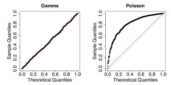
Figure 1: QQ plots of Cox-Snell residuals under correctly specified models. Left panel: gamma regression. Right panel: Poisson regression. The dashed line is the diagonal throughout the paper.

However, if $Y$ is a discrete variable, the Cox-Snell residuals may not be uniformly distributed even under the true model. In the right panel of Figure 1, the data are generated from a Poisson generalized linear model (GLM). It displays the QQ plot of the Cox-Snell residuals when the model is correctly specified, which nevertheless shows a substantial deviation from the diagonal line.

2.2 Proposed Residuals

Our goal is to construct a new type of residuals for discrete outcomes which satisfies the desirable property (1) with a convenient null distribution $F_{r}$. We first study the probability integral transform of discrete outcomes. Given $\mathbf{X}=\mathbf{x}$,

$$\Pr\left(\left.F(Y|\mathbf{X})\leq s\right|\mathbf{X}=\mathbf{x}\right)=\Pr\left(\left.Y\leq F^{(-1)}(s|\mathbf{x})\right|\mathbf{X}=\mathbf{x}\right)=F\left(\left.F^{(-1)}(s|\mathbf{x})\right|\mathbf{x}\right),$$ (2)

where $F^{(-1)}(s|\mathbf{x})\coloneqq\sup\{k\in\mathbb{N}:F(k|\mathbf{x})\leq s\}$. Note that $F^{(-1)}$ differs from the commonly used definition of the inverse cumulative distribution function. For completeness, we let $F^{(-1)}(0|\mathbf{x})=-\infty$. Taking the expectation over $\mathbf{X}$, it follows that

$$G_{0}(s)\coloneqq\Pr\left(F(Y|\mathbf{X})\leq s\right)=\mathrm{E}_{\mathbf{X}}\left[\left.F\left(F^{(-1)}(s|\mathbf{X})\right|\mathbf{X}\right)\right].$$ (3)

We can see that, first, when $Y$ is discrete, the composition $F\left(\left.F^{(-1)}(s|\mathbf{x})\right|\mathbf{x}\right)$ is not necessarily equal to $s$. Consequently, $G_{0}$ in (3) is not the identity function, and thus the probability integral transform is not uniformly distributed, as illustrated in the right panel of Figure 1. Second, if $Y$ is continuous, (3) simplifies to the identity function.

If $\mathbf{X}$ contains continuous components, $F(Y|\mathbf{X})$ becomes a continuous variable as a transform of $\mathbf{X}$ and $Y$; see details in the supplementary material. Although $F(Y|\mathbf{X})$ itself is not uniformly distributed for discrete outcomes, because $F(Y|\mathbf{X})$ is a continuous variable, another layer of probability integral transformation, namely $G_{0}\left(F(Y|\mathbf{X})\right)$, produces a uniform variable under the true model. We call ${r}(Y|\mathbf{X})=G_{0}\left(F(Y|\mathbf{X})\right)$ the double probability integral transform (DPIT for brevity), whose distribution $F_{r}$ is uniform and straightforward to work with. The DPIT serves as our generalized error in (1). A list of the DPIT properties is provided in Appendix A.

With a sample $(\mathbf{X}_{i},Y_{i}),~{}i=1,\ldots,n$, now we construct residuals based on the DPIT. With a model $M$, one could theoretically use ${G}_{0}\left(\hat{F}_{M}(Y_{i}|\mathbf{X}_{i})\right)$, $i=1,\ldots,n$. The distribution of the probability integral transform for a discrete outcome, $G_{0}$, yet remains to be specified and estimated in practice.

Based on (3), an intuitive estimator for ${G}_{0}(s)$ is the empirical mean $\frac{1}{n}\sum_{j=1}^{n}{F}\left(\left.{F}^{(-1)}(s|\mathbf{X}_{j})\right|\mathbf{X}_{j}\right).$ There are two issues to be addressed here. First, this raw estimator depends on $F$, which is unknown in practice. We use the model-based version with estimated parameters plugged in, $\hat{F}_{M}$. Second, when constructing the residual for the $i$th observation, we should estimate ${G}_{0}$ using other independent observations to avoid bias; see elaboration in Appendix A. Taken together, we develop an estimator of $G_{0}$ suited to the $i$th observation

$$\hat{G}_{Mi}(s)=\frac{1}{n-1}\sum_{j=1,j\neq i}^{n}\hat{F}_{M}\left(\left.\hat{F}_{M}^{(-1)}(s|\mathbf{X}_{j})\right|\mathbf{X}_{j}\right).$$ (4)

While $\hat{G}_{Mi}$ is a function defined for $s\in(0,1)$, we only need its value at one point, $\hat{F}_{M}(Y_{i}|\mathbf{X}_{i})$, to develop the residuals.

Combining the components above, we propose the double probability integral transform residuals (DPIT residuals for brevity)

$$\hat{r}(Y_{i}|\mathbf{X}_{i})=\hat{G}_{Mi}\left(\hat{F}_{M}(Y_{i}|\mathbf{X}_{i})\right),i=1,\ldots,n.$$ (5)

If the model is correctly specified, the DPIT residuals should closely follow a uniform distribution (e.g., the right panel of Figure 2), and otherwise model deficiency is implied. To facilitate visualization and comparison with other residuals, one can also apply the normal quantile transformation $\Phi^{-1}$ to the DPIT residuals, resulting in

$$\Phi^{-1}\left[\hat{r}(Y_{i}|\mathbf{X}_{i})\right],i=1,\ldots,n.$$

Consequently, a standard normal distribution serves as the null pattern. In Figure 18 of Appendix B, we demonstrate the behavior of the residuals on both uniform and normal scales in a simulated example, wherein we can see that the uniform residuals accentuate the center values, while the normal residuals emphasize the tails.

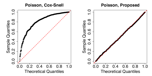
Figure 2: QQ plots of residuals under the correctly specified model.

The construction of the proposed residuals involves two-stage estimation. We need to first estimate the model parameters using all the data to obtain $\hat{F}_{M}$. Subsequently, using the parameter estimates, we estimate $G_{0}$ through $\hat{G}_{Mi}$ for each observation $i$. For the $i$th observation, the corresponding residual can be calculated as follows.

1. Calculate $a_{i}=\hat{F}_{M}(Y_{i}|\mathbf{X}_{i})$.

2. For $j=1,\ldots,n$ and $j\neq i$, calculate $b_{ij}=\hat{F}_{M}^{(-1)}\left(a_{i}|\mathbf{X}_{j}\right)$, and then determine $c_{ij}=\hat{F}_{M}\left(b_{ij}|\mathbf{x}_{j}\right)$.

3. Compute the average of $c_{ij}$ to yield $\hat{r}(Y_{i}|\mathbf{X}_{i})=\frac{1}{n-1}\sum_{j=1,j\neq i}c_{ij}.$ To acquire the residuals on the normal scale, one can further apply $\Phi^{-1}\left[\hat{r}(Y_{i}|\mathbf{X}_{i})\right].$

We construct the DPIT residuals by compressing the Cox-Snell residuals using $\hat{G}_{Mi}$, thereby ensuring the residuals’ uniform distribution for discrete outcomes under the null. Since $\hat{G}_{Mi}$ converges to $G_{0}$ which is a monotone function, the proposed residuals nearly preserve the ordering of the Cox-Snell residuals. As illustrated in Figure 2, $\hat{G}_{Mi}$ brings the Cox-Snell residuals displayed in the left panel to the diagonal in the right panel. Lastly, if $Y$ is continuous, (4) simplifies to the identity function, and thus the proposed residuals coincide with Cox-Snell residuals. Hence, Cox-Snell residuals for continuous data can be viewed as a special case of the proposed residuals.

2.3 Handling Ordinal and Binary Outcomes

For ordinal outcomes including binary, the probability integral transform $F(Y|\mathbf{X})$ is situated at 1 if $Y$ takes the largest possible value. Suppose the possible values of $Y$ are $0,1,\ldots,k_{\max}$, then $F(Y|\mathbf{X})$ has a point mass at 1 with probability

$$\Pr\left(F(Y|\mathbf{X})=1\right)=\Pr\left(Y=k_{\max}\right)=1-\mathrm{E}_{\mathbf{X}}F({k_{\max}-1}|\mathbf{X}).$$

The distribution of the DPIT is

$$\Pr\left(G_{0}(F(Y|\mathbf{X}))\leq s\right)=\begin{cases*}1&$s=1$,\\ \mathrm{E}_{\mathbf{X}}F({k_{\max}-1}|\mathbf{X})&$\mathrm{E}_{\mathbf{X}}F({k_{\max}-1}|\mathbf{X})<s<1,$\\ s&$s\leq\mathrm{E}_{\mathbf{X}}F({k_{\max}-1}|\mathbf{X})$.\end{cases*}$$

See derivations in the supplementary material. We can see from the equation above that for $\mathrm{E}_{\mathbf{X}}F({k_{\max}-1}|\mathbf{X})<s<1,$ $\Pr\left(G_{0}(F(Y|\mathbf{X}))\leq s\right)$ does not vary with $s$. Consequently, when constructing QQ plots, the quantiles of $G_{0}(F(Y|\mathbf{X}))$ with a probability $s>\mathrm{E}_{\mathbf{X}}F({k_{\max}-1}|\mathbf{X})$ clump at 1. Hence, this area is not helpful for model assessment. As demonstrated in the left panel of Figure 3, in which the simulated outcomes are binary and the model is correctly specified, a cluster of points appears at 1. The points corresponding to the observations whose response variable takes value at 0, in contrast, closely align with the diagonal and provide a correct signal.

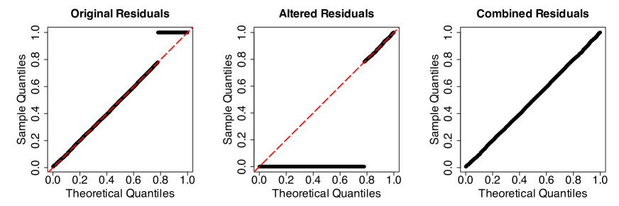
Figure 3: QQ plots of the proposed residuals for binary outcomes with a correctly specified model.

To make full use of the data, we consider an altered DPIT, ${H}_{0}\left({F}(Y-k_{\max}|\mathbf{X}_{i})\right)$, wherein $H_{0}(s)\coloneqq\Pr\left(F(Y-k_{\max}|\mathbf{X})\leq s\right)=\mathrm{E}_{\mathbf{X}}\left[F\left(F^{(-1)}(s|\mathbf{X})+k_{\max}|\mathbf{X}\right)\right].$ The corresponding altered residuals are

$$\hat{r}_{S}(Y_{i}|\mathbf{X}_{i})=\hat{H}_{Mi}\left(\hat{F}_{M}(Y_{i}-k_{\max}|\mathbf{X}_{i})\right)$$ (6)

where

$$\hat{H}_{Mi}(s)=\frac{1}{n-1}\sum_{j=1,j\neq i}^{n}\hat{F}_{M}\left(\hat{F}_{M}^{(-1)}(s|\mathbf{X}_{j})+k_{\max}|\mathbf{X}_{j}\right).$$

In the middle panel of Figure 3, we display the altered residuals, which exploit the information of the data with outcomes equal to 1. The observations whose responses are 0, on the other hand, do not provide information in this case.

To integrate, we combine both types of residuals for ordinal outcomes. One should use the original DPIT residuals for observations smaller than the largest possible value and employ the altered residuals for observations taking value at the maximum. By doing so, we obtain residuals whose null distribution is uniform on $(0,1)$. In the right panel of Figure 3, the residual plot utilizes all the data and is close to the diagonal with a correctly specified model.

2.4 Large Sample Properties

In this section, we study the asymptotic distribution of the proposed residuals. In particular, we look into the empirical residual distribution function

$$\frac{1}{n}\sum_{i=1}^{n}1\left[\hat{r}(Y_{i}|\mathbf{X}_{i})\leq s\right]=\frac{1}{{n}}\sum_{i=1}^{n}1\left[\hat{G}_{Mi}\left(\hat{F}_{M}(Y_{i}|\mathbf{X}_{i})\right)\leq s\right].$$

We focus on the null behavior of the proposed tool, namely when the model is correctly specified $F=F_{M}$. For clarity, we index functions by their parameters $\bm{\beta}$ in this section. The underlying parameters $\bm{\beta}_{0}$ are estimated using the maximum likelihood estimator $\hat{\bm{\beta}}$. The quantity of interest to study is then

$$\frac{1}{\sqrt{n}}\sum_{i=1}^{n}\left\{1\left[\hat{G}_{\hat{\bm{\beta}}i}\left({F}(Y_{i}|\mathbf{X}_{i},\hat{\bm{\beta}})\right)\leq s\right]-s\right\}.$$ (7)

where

$$\hat{G}_{\hat{\bm{\beta}}i}(s)=\frac{1}{n-1}\sum_{j=1,j\neq i}^{n}{F}\left(\left.{F}^{(-1)}(s|\mathbf{X}_{j},\hat{\bm{\beta}})\right|\mathbf{X}_{j},\hat{\bm{\beta}}\right).$$

Theorem 2.1.

Under Assumptions A.1, A.2, and A.3, when the model is correctly specified, for fixed $s$, $\frac{1}{\sqrt{n}}\sum_{i=1}^{n}\left\{1\left[\hat{G}_{\hat{\bm{\beta}}i}\left({F}\left(Y_{i}|\mathbf{X}_{i},\hat{\bm{\beta}}\right)\right)\leq s\right]-s\right\}$ converges weakly to a Gaussian distribution. Its mean is $\mathrm{E}g_{s}(\mathbf{X},Y)$ and variance is $\mathrm{E}g_{s}(\mathbf{X},Y)^{2}-\left(\mathrm{E}g_{s}(\mathbf{X},Y)\right)^{2}$, where

$$g_{s}(\mathbf{x},y)=f_{s}(\mathbf{x},y)+\left[I(\bm{\beta}_{0})\right]^{-1}\left.\frac{\partial\left[\tilde{G}_{\bm{\beta},\bm{\beta}_{0}}\left(G_{\bm{\beta}}^{-1}(s)\right)\right]}{\partial\beta}\right|_{\beta=\bm{\beta}_{0}}\dot{l}_{\bm{\beta}_{0}}(\mathbf{x},y),$$

and

$$f_{s}(\mathbf{x},y)=1\left(G_{0}(F(y|\mathbf{x},\bm{\beta}_{0}))\leq s\right)-F\left(\left.F^{(-1)}(G_{0}^{-1}(s)|\mathbf{x},\bm{\beta}_{0})\right|\mathbf{x},\bm{\beta}_{0}\right).$$

Furthermore,

$$\tilde{G}_{\bm{\beta},\bm{\beta}_{0}}(s)\coloneqq\Pr\left(F(Y|\mathbf{X},\bm{\beta})\leq s\right)=\mathrm{E}_{\mathbf{X}}\left[F\left(\left.F^{(-1)}(s|\mathbf{X},\bm{\beta})\right|\mathbf{X},\bm{\beta}_{0}\right)\right];$$ (8)

$I(\beta)$ is the Fisher information matrix; ${l}_{\beta}(\mathbf{x},y)$ is the log-likelihood, and $\dot{l}_{\bm{\beta}}(\mathbf{x},y)=\partial l_{\bm{\beta}}(\mathbf{x},y)/\partial\bm{\beta}$ is the score function.

From Theorem 2.1, we can see that the proposed residuals do converge to being uniformly distributed asymptotically, at the order of $\sqrt{n}$. Furthermore, the uncertainties associated with the distribution of the proposed residuals originate from two distinct sources. The first part $f_{s}(\mathbf{x},y)$ arises from the estimation of $G_{0}$, and the second part involves the uncertainty in $\hat{\bm{\beta}}$. The details and proof of the theorem are provided in the supplementary material.

3 Ordered Curve

Reflecting on (2), the distribution of the probability integral transform varies with the value of $\mathbf{x}$ for discrete outcomes. When constructing the proposed residuals, despite an overall transformation $G_{0}$, the dependence of the DPIT on covariates remains. As will be demonstrated in the simulation study, the residuals versus predictor plots are not informative. Therefore, the DPIT residuals have limited capacity of detecting deficiency in the mean structure. In this section, we propose a supplementary tool for assessing mean structures.

Lorenz curves (Hand and Henley 1997), a concept originally employed to compare risk classifiers in finance, were adapted by Frees et al. (2011) to judge the adequacy of insurance premiums. In their framework, Lorenz curves compare the cumulative sum of premiums with the cumulative sum of actual losses, as a threshold changes. Here we generalize this idea to assess the mean structure of discrete outcomes.

In order to assess the mean structure, we propose to compare the cumulative sum of the response variable $Y$ and its hypothesized value. Denote the mean for the $i$th observation as $\lambda_{i}$, and $\hat{\lambda}_{i}$ is the fitted value. For instance, in a Poisson GLM with a log link, $\lambda_{i}=\exp\left(\mathbf{X}_{i}^{\prime}\bm{\beta}\right)$. Note that for ordinal outcomes, it requires the assignment of numbers to categories, and $\lambda_{i}$ is the mean based on the integer encoding of categories. We further let $\Lambda$, which is a transform of $\mathbf{X}$, be the random variable generating $\lambda_{i}$. We introduce a variable denoted as $Z$ to determine the cutoff. Here $Z$ can be $\Lambda$ itself, a linear combination of $\mathbf{X}$, or a variable outside $\mathbf{X}$. We will discuss below the choice of $Z$. On the one hand, the cumulative response function is defined as

$$L_{1}(t)=\frac{\mathrm{E}\left[Y1(Z\leq t)\right]}{\mathrm{E}\left[Y\right]},$$

with its empirical counterpart being

$$\hat{L}_{1}(t)=\frac{\sum_{i=1}^{n}\left[Y_{i}1(Z_{i}\leq t)\right]}{\sum_{i=1}^{n}Y_{i}}.$$

The function is divided by the sum of the responses for normalization. On the other hand, assuming the model is correct, if $Z$ is either contained in $\mathbf{X}$ or independent of $\mathbf{X}$ and $Y$,

$$\mathrm{E}\left[Y1(Z\leq t)\right]=\mathrm{E}\left[\Lambda 1(Z\leq t)\right];$$

see Appendix A for details. In either case, we define

$$L_{2}(t)=\frac{\mathrm{E}\left[\Lambda 1(Z\leq t)\right]}{\mathrm{E}\Lambda}.$$

Its empirical version is

$$\hat{L}_{2}(t)=\frac{\sum_{i=1}^{n}\left[\hat{\lambda}_{i}1(Z_{i}\leq t)\right]}{\sum_{i=1}^{n}\hat{\lambda}_{i}}.$$

If the mean structure is correctly specified, namely $\Lambda$ is indeed the mean of $Y$, we expect that $L_{1}$ and $L_{2}$ are close to each other. Therefore, in practice, we can examine the curve $(\hat{L}_{2}(t),\hat{L}_{1}(t))$, as $t$ varies. If the curve is distant from the diagonal, it suggests discrepancies between $L_{1}$ and $L_{2}$ and thus incorrectness in the mean structure. In addition, the position of the curve relative to the diagonal reveals the relationship between the fitted and underlying means. If the curve lies above the diagonal, it indicates that the cumulative sum of the response is larger than that of the fitted mean, and thus the mean is underestimated, and vice versa.

This idea of comparing the estimated mean to the mean of the outcome is used to construct calibration plots for classifiers. To do so, the fitted probabilities are typically binned (Faraway 2016). To avoid the ad-hoc nature of binning, we consider the cumulative sum instead. Su and Wei (1991) used the partial sums of residuals over a partition of the covariate space. However, their method required simulations to establish the null behavior of the tool.

To pragmatically construct the ordered curve, one can order the threshold variable $Z_{(1)},Z_{(2)},\ldots,Z_{(n)}$ and denote the original index of $Z_{(i)}$ as $T_{i}$. That is, $Z_{(i)}=Z_{T_{i}}$. The empirical version of the curve $\hat{L}_{1}(t)$ against $\hat{L}_{2}(t)$ can then be characterized by the following $n$ points

$$\left(\frac{\hat{\lambda}_{T_{1}}}{\sum_{i=1}^{n}\hat{\lambda}_{i}},\frac{Y_{T_{1}}}{\sum_{i=1}^{n}Y_{i}}\right),\left(\frac{\hat{\lambda}_{T_{1}}+\hat{\lambda}_{T_{2}}}{\sum_{i=1}^{n}\hat{\lambda}_{i}},\frac{Y_{T_{1}}+Y_{T_{2}}}{\sum_{i=1}^{n}Y_{i}}\right),\ldots,\left(\frac{\sum_{i=1}^{k}\hat{\lambda}_{T_{i}}}{\sum_{i=1}^{n}\hat{\lambda}_{i}},\frac{\sum_{i=1}^{k}Y_{T_{i}}}{\sum_{i=1}^{n}Y_{i}}\right),\ldots,\left(1,1\right).$$

In GLMs, as a result of the normal equation, $\sum_{i=1}^{n}\hat{\lambda}_{i}$ and $\sum_{i=1}^{n}Y_{i}$ are typically very close. Hence, the denominators of $\hat{L}_{1}$ and $\hat{L}_{2}$ serve as normalization factors and do not impact the shape of the curve much.

The role of the threshold variable $Z$ is to determine the rule for accumulating $\Lambda$ and $Y$ for the ordered curve. The candidates for $Z$ include first the fitted values, second a linear combination of $\mathbf{X}$, or third a potential variable to be included as a covariate. In the third case, if the variable being considered is in fact irrelevant, it is equivalent to randomly reordering the data and calculating the partial sums.

To reveal a potential lack of fit, the optimal choice for $Z$ should lead to a significant separation between $\Lambda$ and $Y$. Assuming no collinearity, an important predictor which is missing in the model can induce such an effect, since it is highly correlated with $Y$ but not with $\Lambda$. Therefore, if a variable leads to a large discrepancy between the ordered curve and the diagonal, including this variable in the mean function should be considered.

4 Simulation

In this section, we discuss the operating characteristics of the proposed tools via various examples. In Section 4.1, we show that the proposed residuals exhibit null patterns when the model is correctly specified. In Section 4.2, we explore their behaviors when the model is misspecified. In Section 4.3, the empirical performance of the ordered curve is evaluated.

4.1 Closeness to Null Pattern under True Models

We first demonstrate that when the model is correctly specified, the proposed residuals follow the null pattern. In Figure 4, the data are generated using a negative binomial distribution with mean $\mu=\exp\left(\beta_{0}+X_{1}\beta_{1}+X_{2}\beta_{2}\right)$, where $X_{1}\sim N(0,1)$, and $X_{2}$ is binary with a probability of success as 0.7. The coefficients are set as $\beta_{0}=-2,\beta_{1}=2$, and $\beta_{2}=1$. The underlying size parameter is 2. We vary the sample size from 50 to 500. For visual clarity and comparability with other residuals, we present our residuals on the normal scale $\Phi^{-1}\left[\hat{r}(Y_{i}|\mathbf{X}_{i})\right]$ in this section, and thus a standard normal distribution is the null pattern.

In the left column of Figure 4, when the model is correctly specified, the QQ plots of the proposed residuals are in close proximity to the diagonal (dashed line throughout this section), indicating that they closely follow the null distribution. This behavior persists even when the sample size is rather small in the top row. This is an advantage of the proposed residuals over the tool in Yang (2021), which utilizes kernel functions and requires a large sample size. For comparison, we also display the normal QQ plots of deviance and Pearson residuals. They deviate from the null pattern and erroneously signal a deficiency in the model, leading to a Type I error.

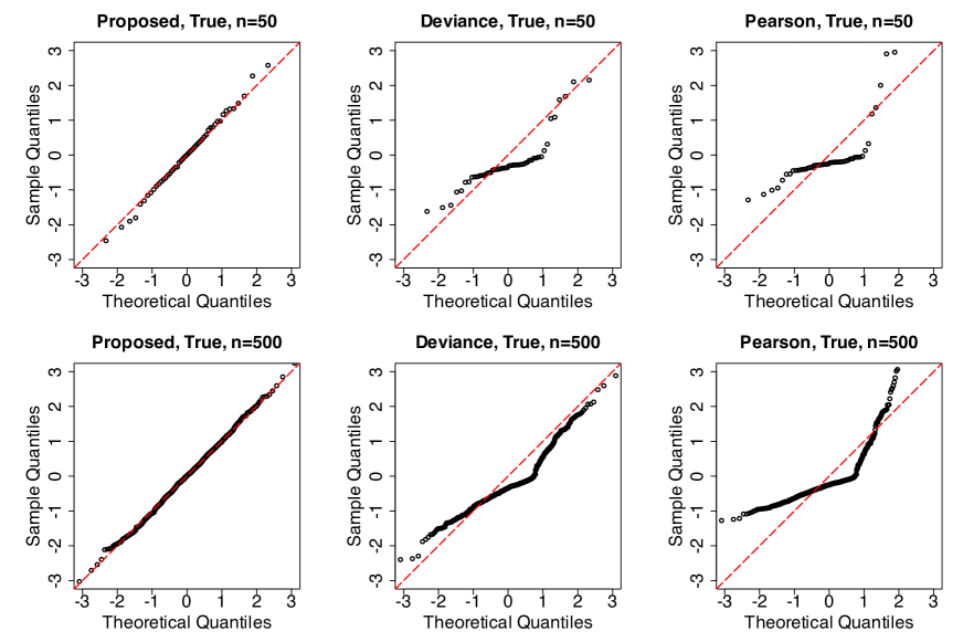
Figure 4: QQ plots of the proposed residuals (left column) compared with deviance (middle column) and Pearson residuals (right column) when the model is correctly specified. The sample size is 50 in the top row and 500 in the second row.

We further compare the proposed residuals with the randomized quantile residuals in Figure 5. The randomness associated with randomized quantile residuals is particularly evident for small sample sizes. For the same dataset and model, we see distinct patterns in the randomized quantile residuals with different seed numbers, as shown in the middle and right panels.

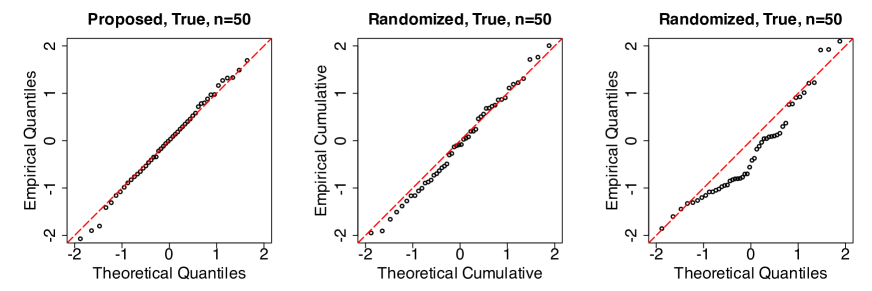
Figure 5: QQ plots of the proposed residuals (left) and randomized quantile residuals (middle and right panels, with different seed numbers) for negative binomial outcomes with a correctly specified model.

To assess the variability of the proposed residuals, we further present a simulation study with 10000 replicates in the supplementary material. It shows that our residuals are close to being normally distributed under small sample sizes. To save space, the null patterns of the proposed residuals under other distributions are displayed in the comparative plots of Section 4.2.

4.2 Discrepancy with the Null When the Model Is Misspecified

In this section, we demonstrate that the proposed residuals can effectively detect model misspecification in various scenarios. Sample sizes are 500 throughout this section.

4.2.1 Overdispersion and Zero-Inflation in Count Data

For the negative binomial data described in Section 4.1, now we fit them with a Poisson GLM, and thus overdispersion is present. The resulting QQ plots of the proposed residuals, along with other residuals, are shown in the bottom row of Figure 6. In the first column, we can see that the proposed residuals show a transition from being close to the diagonal when the model is correctly specified to displaying an obvious and readily interpretable discrepancy when overdispersion is an issue. In contrast, the deviance and Pearson residuals show a large discrepancy with the null pattern in both scenarios, making them not informative.

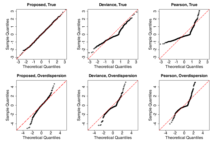
Figure 6: QQ plots of the proposed residuals (left column) compared with deviance (middle column) and Pearson residuals (right column) for negative binomial data. The model is correctly specified in the first row, while in the second row, the data are mistakenly fit with a Poisson GLM.

In Appendix B.1, we illustrate that the shape of the QQ plot for the proposed residuals is determined by the relationship between the estimated distribution function $\hat{F}_{M}$ and the true distribution function $F$. Due to the orthogonality between the mean and dispersion components in GLMs, the mean structure is close to being correctly fit even when the dispersion parameter is misspecified. In an overdispersed model, due to the underestimated variance, $\hat{F}_{M}$ behaves more wildly than $F$. Therefore, if one spots the S-shaped pattern in the QQ plot, as shown in the lower left panel of Figure 6, it is probable that overdispersion is an issue.

Besides negative binomial distributions, zero-inflated models are commonly used to handle overdispersion in count data. In Figure 7, we simulate data using a zero-inflated Poisson model. The probability of excess zeros is modeled with $\mathrm{logit}(p_{0})=\beta_{00}+\beta_{10}X_{1}$, and the Poisson component has a mean $\lambda=\exp(\beta_{0}+\beta_{1}X_{1}+\beta_{2}X_{2})$, where $X_{1}\sim N(0,1)$ and $X_{2}$ is a dummy variable with a probability of 1 equal to 0.7, and $(\beta_{00},\beta_{10},\beta_{0},\beta_{1},\beta_{2})=(-2,2,-2,2,1)$. In the top row of Figure 7, when the model is correctly specified, the proposed residuals closely follow their null pattern. In contrast, the deviance and Pearson residuals again deviate from normality. Here the saturated Poisson model is used to define the deviance residuals for the zero-inflated Poisson model (Lee et al. 2001). When the model is misspecified, as depicted in the bottom row of Figure 7, the proposed residuals show a large discrepancy from the diagonal. Moreover, a noticeable S-shaped pattern, similar to what was observed in the bottom left panel of Figure 6, arises due to overdispersion.

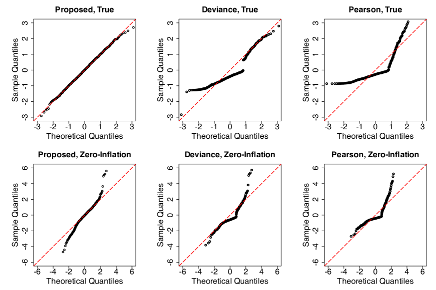
Figure 7: QQ plots of the proposed residuals (left column) compared with the deviance (middle column) the Pearson residuals (right column) for zero-inflated Poisson data. The model is correctly specified in the top row and misspecified as a Poisson GLM in the bottom row.

4.2.2 Ordinal Data

In this experiment, we consider ordinal regression models with three levels 0, 1, and 2. Under an ordinal logistic regression model with proportionality assumption, $P(Y\leq j)=F(\alpha_{j}),$ where $F$ is the distribution function of a logistic random variable with mean $\beta_{1}X_{1}$. We let $\alpha_{0}=1$, $\alpha_{1}=4$, $\beta_{1}=3$, and $X_{1}\sim N(2,1)$.

Here we compare the proposed method with the two types of residuals introduced in Li and Shepherd (2012) and Liu and Zhang (2018) which were designed to tackle ordinal regression model diagnostics. In Liu & Zhang framework, it is assumed that there is a latent variable $A_{i}$ which follows a logistic distribution with mean $X_{i1}\hat{\bm{\beta}}_{1}$. Given the fitted thresholds $\hat{\alpha}_{0}$ and $\hat{\alpha}_{1}$, they simulate the residual $\hat{r}_{i}^{\text{Liu}}$ from the distribution of $A_{i}|Y_{i}=y_{i}$. Under the correct model, these residuals are expected to follow a logistic distribution. The Li & Shepherd residuals are defined as $\hat{r}_{i}^{\text{Li}}=\hat{F}(Y_{i}-1|\mathbf{X}_{i})+\hat{F}(Y_{i}|\mathbf{X}_{i})-1$. For continuous outcomes, these residuals are supposed to follow a uniform distribution over $[-1,1]$ under the true model. We can see in the top row of Figure 8 that both the proposed method and the Liu & Zhang residuals result in plots that are closely aligned with the diagonal when the model is correctly specified.

We then generate data under the scenario where the assumption of proportionality is not met, which is a common issue for ordinal regression models. Specifically, $P(Y\leq 0)=F(\alpha_{0})$ as described above whereas $P(Y\leq 1)=F_{1}(\alpha_{1})$, where $F_{1}$ is the distribution function of a logistic random variable with mean $\beta_{2}X_{1}$ and we set $\beta_{2}=1$. The data are incorrectly fit with a proportional odds model, and the bottom row of Figure 8 includes the results. It is apparent that our proposed method demonstrates sensitivity to the presence of non-proportionality in this example.

To explore the shape of the QQ plot, in the supplementary material, we compare the underlying and fitted probabilities under non-proportionality. The fitted probabilities of zeros and the fitted cumulative probabilities at $k_{\max}-1$ are consistently larger than the corresponding underlying probabilities, resulting in a QQ plot with both tails above the diagonal, as shown in the lower left panel of Figure 8.

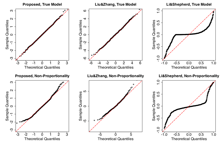
Figure 8: Graphical detection of non-proportionality in ordinal regression models. The two rows correspond to scenarios in which the assumption of proportionality is met and not met, respectively.

4.2.3 Binary

We further include an example of binary data. The underlying model is a logistic regression with the probability of 1 as $\mathrm{logit}^{-1}(\beta_{0}+\beta_{1}X_{1}+\beta_{2}X_{2}+\beta_{3}X_{1}X_{2})$, where $(\beta_{0},\beta_{1},\beta_{2},\beta_{3})=(-5,2,1,3)$, $X_{1}\sim N(1,1)$, and $X_{2}$ is a dummy variable with a probability of one equal to 0.7. For the misspecified model, the binary covariate and the interaction term are omitted. It was discussed in Hosmer et al. (1997) that most goodness-of-fit tests tend to have limited power in such settings. Figure 9 shows the results. Due to the undesirable properties of deviance and Pearson residuals, here we display Liu & Zhang and Li & Shepherd residuals instead. When the model is correctly specified, the proposed residuals follow the null pattern. When the interaction term is omitted, on the other hand, the proposed tool can effectively detect the model deficiency.

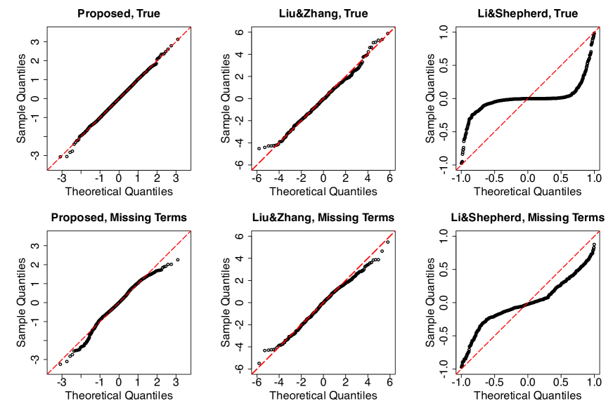
Figure 9: QQ plots of the proposed residuals (left column) compared with the Liu & Zhang residuals (middle column) and Li & Shepherd residuals (right column) for the binary example. The model is correctly specified in the top row and a main effect and an interaction term are missing in the bottom row.

4.2.4 Outliers

The proposed residuals can help identify outliers. Figure 10 includes a Poisson example, with the same underlying mean structure as the negative binomial outcomes discussed in Section 4.1. We manually enlarged three outcomes by adding values of $10,~{}15,$ and $20$ to them, respectively. In the left panel of Figure 10, we can see the three modified data points stand out, signaling they are potential outliers.

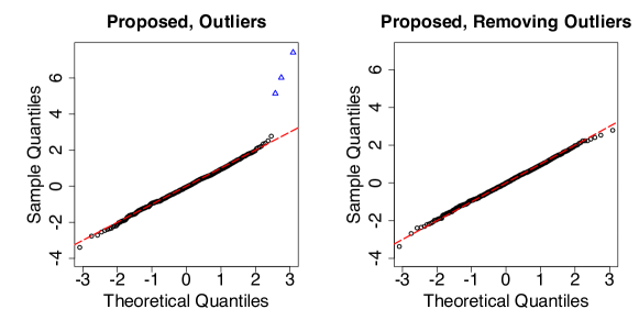
Figure 10: Graphical detection of outliers.

We also emphasize that close examination of the data is required for outlier identification. As will be demonstrated in the next section, the distribution of the proposed residuals depends on the values of covariates. Therefore, it is possible that a large value of the residual is the consequence of high leverage. When encountering suspected cases, it is important to carefully examine the data.

4.2.5 Limitation: Uninformative Residuals Versus Predictor Plots

In linear regression models, another common utility of residuals is to check the mean structure. Analysts routinely check residuals versus predictor plots to decide whether the covariate structure is sufficient or if another variable should be included in the model. As discussed in Section 3, the distribution of the proposed residuals depends on the value of covariates. In the left column of Figure 11, we display the residuals versus fitted values plots for the negative binomial (NB) and binary examples of Sections 4.2.1 and 4.2.3, respectively, when the model is correctly specified. The fitted values are on the scale of the linear predictors. It is clear that the distribution of the residuals changes with the fitted values, and we should not expect the residuals to exhibit no discernible pattern. In addition, we differentiate the residuals based on the corresponding outcomes. We can see that the residuals show lines of points corresponding to the observed responses, as noted in Faraway (2016). It was shown in the literature that other residuals, including Pearson, deviance and Li & Shepherd residuals, also face this challenge for discrete data (Shepherd et al. (2016); Liu and Zhang (2018); Liu et al. (2021)), which we illustrate in the right column of Figure 11. In order to assess the mean structure, we proposed a tool in Section 3. We will demonstrate its utility in the next section.

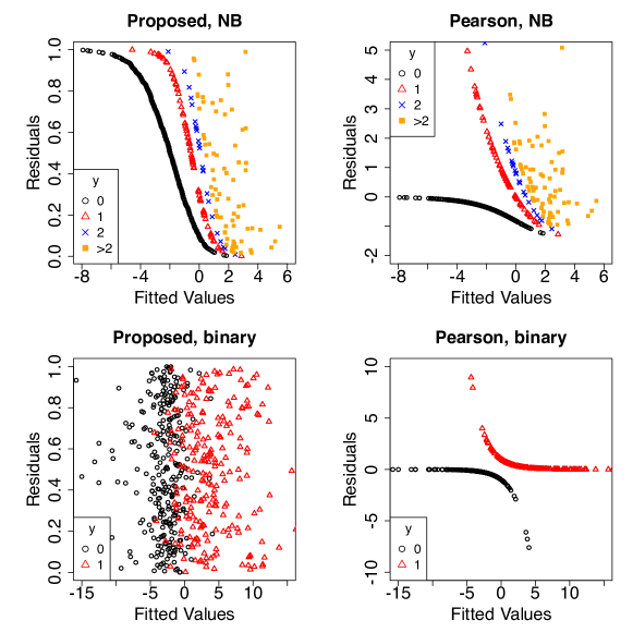
Figure 11: Residual versus fitted value plots when the model is correctly specified.

4.3 Ordered Curve

We first revisit the binary example in Figure 9. In each plot of Figure 12, we display the ordered curves for both the correctly specified (solid curve) and the misspecified model (dotted curve). We consider three different choices for the threshold variable $Z$, the fitted values (left panel), the missing covariate (middle panel), and a randomly simulated irrelevant variable (right panel). We can see that, first, regardless of the threshold variable, when the mean structure is correctly specified, the solid curves are close to the diagonal (dashed line). Second, for the misspecified model, the degree of deviation between the ordered curve and the diagonal depends on the choice of the threshold variable. When we use the fitted values to sort the data, the curve for the incorrect model shows a small deviation from the diagonal. Strikingly, when the omitted variable $X_{2}$ is used as the threshold variable, it leads to a curve far from the diagonal. On the other hand, if $Z$ is a completely irrelevant variable, we can hardly detect the incorrectness in the mean structure.

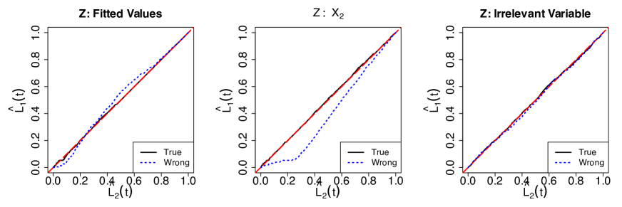
Figure 12: Ordered curves of binary regression with different threshold variables $Z$. The sample size is 500.

We further explore a Poisson example. The mean function is $\mu=\exp\left(\beta_{0}+X_{1}\beta_{1}+X_{2}\beta_{2}\right)$, where $X_{1}$ and $X_{2}\sim N(0,1)$ independently. The coefficients are set to be $\beta_{0}=0,\beta_{1}=2$, and $\beta_{2}=1$. For the misspecified model, $X_{2}$ is omitted. Consistent with our observations of Figure 12, using the omitted variable as the threshold variable elucidates the distinction between the fitted means and the means of the actual outcomes. When we use the fitted values and an irrelevant variable as the threshold variable, we observe a slight deviation from the diagonal under the misspecified model in this example.

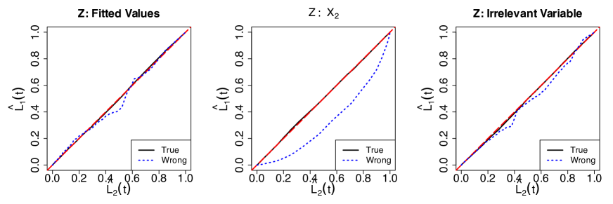
Figure 13: Ordered curves of Poisson regression with different threshold variables $Z$. The sample size is 500.

5 Data Analysis

In this section, we present real data examples to demonstrate the workflow of model assessment using our tools.

5.1 Count Data

AT&T ran an experiment varying five factors relevant to a wave-soldering procedure for mounting components on printed circuit boards (Comizzoli et al. 1990). The response variable is the count of how many solder skips appeared to a visual inspection. Table 1 includes the description and summary statistics of the important covariates. The sample size is 900. This example demonstrates the application of the proposed residuals even in cases where continuous covariates are not present, as long as there are factors with many levels.

Table 1: Covariates of AT&T data.

Variable	Description	Levels (Frequency)
Opening	the amount of clearance around the	L (300), M (300), S (300)
	mounting pad
Solder	the amount of solder	Thick (450), Thin (450)
Mask	type and thickness of the material	A1.5 (180), A3 (270),
	used for the solder mask	A6 (90), B3 (180), B6 (180)
PadType	the geometry and size of the	D4 (90), D6 (90), D7 (90),
	mounting pad	L4 (90), L6 (90), L7 (90),
		L8 (90), L9 (90), W4 (90),
		W9 (90)
Panel	each board was divided into 3 panels	1 (300), 2 (300), 3 (300)

We first fit regression models with main effects. In the left panel of Figure 14, we use a Poisson GLM, and our tool displays a pronounced S-shaped pattern, hinting at potential overdispersion. This is consistent with the conclusion of Faraway (2016). In the middle panel, we use a negative binomial distribution to correct for overdispersion. According to our residuals, the negative binomial distribution leads to a substantial improvement in the model fit, yet some insufficiency is indicated by the tails. In the right panel, we analyze the ordered curve, which implies insufficiency in the mean structure.

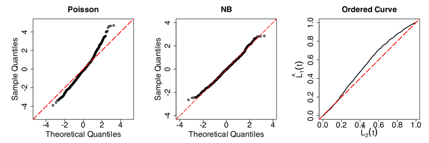
Figure 14: Assessment plots for the regression models of the solder data with main effects only. The left and middle panels display the proposed residuals of Poisson and negative binomial regressions, respectively. The right panel shows the ordered curve and the fitted values are used as the threshold variable.

We then include interaction terms selected using a stepwise procedure. Figure 15 shows the diagnostic plots of the resulting model. The inclusion of interaction terms yields a considerable improvement in model fit.

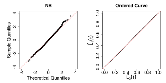
Figure 15: Assessment plots for the negative binomial models of the solder data with main effects and interactions.

5.2 Binary Outcomes

The dataset was collected in one of the earliest studies addressing the factors impacting the chance of developing heart disease (Rosenman et al. 1975). The study started in 1960 and involved 3154 healthy men aged between 39 and 59. All the subjects were free of heart disease at the beginning of the study. The response variable is whether these men developed heart disease eight and a half years later. 255 men developed coronary heart disease, while the others did not. Table 2 includes the variables that might be related to the chance of developing this disease.

Table 2: Covariates of heart data.

Variable	Description	Mean (sd) / Levels (count)
age	age in years	46.275 (5.517)
height	height in inches	69.780 (2.521)
sdp	systolic blood pressure in mm Hg	128.603 (15.056)
chol	fasting serum cholesterol in mm %	226.346 (43.421)
behave	behavior type which is a factor	A1 (263), A2 (1320), B3 (1209),
		B4 (348)
cigs	number of cigarettes smoked per day	11.577 (14.494)
arcus	arcus senilis	absent (2202), present (938)
bmi	body mass index	24.516 (2.564)

We first highlight the difficulties in the assessment of regression models with binary outcomes. We fit the data with all the variables except age, which is a very important predictor clinically. Figure 16 includes the proposed residual plot (left panel) and the randomized quantile residual plot (right panel). The proposed residuals have a slight deviation from the diagonal at the upper tail, while the randomized quantile residuals indicate that the model is sufficient. This is further supported by the Hosmer-Lemeshow test (Hosmer and Lemeshow 1980), which returns a large p-value 0.62, suggesting the adequacy of the model. Since the data are fit with logistic regression, a calibration plot is not revealing either.

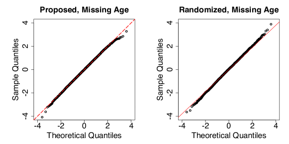
Figure 16: Residual plots for logistic regression of the heart disease data with the variable age missing. Left: QQ plot of the proposed residuals. Right: QQ plot of randomized quantile residuals.

However, in the left panel of Figure 17, we show the ordered curve when age is used as the threshold variable. The curve clearly suggests that the mean structure is insufficient and age should be considered as a predictor, which is consistent with common knowledge. In the right panel of Figure 17, we include age as a predictor, and the ordered curve suggests an improvement in the mean structure.

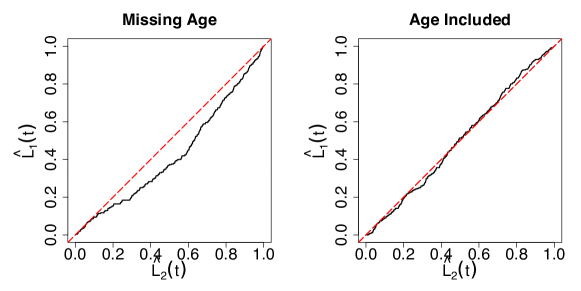
Figure 17: Ordered curves for logistic regression of the heart disease data. Left: age is not included in the mean and age is used as the threshold variable. Right: age is included and fitted values are used as the threshold variable.

6 Conclusion

Regression models with discrete outcomes are commonly used in a wide range of areas. Diagnostics for such models are challenging due to the lack of effective tools. In this paper, we proposed the DPIT residuals to assess regression models with discrete outcomes. To further assess the mean structure, we also proposed an ordered curve, and we showed in the data analysis that it can reveal model deficiency overlooked by other tools. We focused on diagnostics and informal assessment in this paper. Goodness-of-fit tests (e.g., Hosmer et al. 1997; Nattino et al. 2020) which provide p-values and statements with statistical confidence will be investigated in the future.

To summarize the workflow of model assessment using the proposed tools, one should first look into the QQ plot of the DPIT residuals for overall assessment. Meanwhile, one should examine the ordered curve to evaluate the mean structure. We recommend using the fitted values and potential predictors as the threshold variable. If one variable leads to a large discrepancy between the ordered curve and the diagonal, this variable should be considered to include in the mean function. On the other hand, if the mean structure seems sufficient yet the residual plot indicates model deficiencies, one can identify causes of misspecification from the shape of the QQ plot. For instance, an S-shaped QQ plot for count data might hint at overdispersion, while a U-shaped plot for ordinal outcomes might imply non-proportionality. This can also be combined with tools devoted to specific types of misspecification (e.g., Pregibon (1981)). We note that in practice, we might incur more than one type of misspecification simultaneously, and the causes of misspecification are not always identifiable (Cook and Weisberg 1999). The regression model-building process should therefore involve iterations between assessment and improvement.

Appendix A Additional Derivations

Under the true model, the following properties hold for the DPIT.

1. $\mathrm{E}\left\{{r}(Y|\mathbf{X})\right\}=\frac{1}{2}.$ On the normal scale, $\mathrm{E}\left\{\Phi^{-1}\left[{r}(Y|\mathbf{X})\right]\right\}=0.$

2. $\mathrm{Var}\left\{{r}(Y|\mathbf{X})\right\}=\frac{1}{12}.$ On the normal scale, $\mathrm{Var}\left\{\Phi^{-1}\left[{r}(Y|\mathbf{X})\right]\right\}=1.$

3. For $y_{1}\leq y_{2}$,

   $${r}(y_{1}|\mathbf{X})\leq{r}(y_{2}|\mathbf{X}).$$

The third property holds since both $F(\cdot|\mathbf{X})$ and $G_{0}(\cdot)$ are non-decreasing functions. With parameter estimates plugged in, the residuals resemble the DPIT, which we show in Section 2.4.

We now elucidate the construction of $\hat{G}_{Mi}$ in (4). If we were to use all the observations, the estimated DPIT of the $i$th outcome is

$$\frac{1}{n}\sum_{j=1}^{n}{F}\left({F}^{(-1)}(\left.{F}(Y_{i}|\mathbf{X}_{i})\right|\mathbf{X}_{j})|\mathbf{X}_{j}\right)$$

$$= \frac{1}{n}\sum_{j=1,j\neq i}^{n}{F}\left(\left.{F}^{(-1)}({F}(Y_{i}|\mathbf{X}_{i})|\mathbf{X}_{j})\right|\mathbf{X}_{j}\right)+\frac{1}{n}{F}\left(\left.{F}^{(-1)}\left({F}(Y_{i}|\mathbf{X}_{i})|\mathbf{X}_{i}\right)\right|\mathbf{X}_{i}\right)$$

$$= \frac{1}{n}\sum_{j=1,j\neq i}^{n}{F}\left(\left.{F}^{(-1)}({F}(Y_{i}|\mathbf{X}_{i})|\mathbf{X}_{j})\right|\mathbf{X}_{j}\right)+\frac{{F}(Y_{i}|\mathbf{X}_{i})}{n}.$$

The first term in this display resembles ${G}_{0}\left({F}(Y_{i}|\mathbf{X}_{i})\right)$, the DPIT. The second term, however, induces bias from ${G}_{0}\left({F}(Y_{i}|\mathbf{X}_{i})\right)$. Hence, we ought to exclude the $i$th observation.

Next, we derive the $L_{2}(t)$ function for ordered curves. If $Z$ is contained in $\mathbf{X}$, the cumulative response equals

$$\mathrm{E}\left[Y1(Z\leq t)\right]=\mathrm{E}_{\mathbf{X}}\mathrm{E}\left[Y1(Z\leq t)|\mathbf{X}\right]=\mathrm{E}_{\mathbf{X}}\left[1(Z\leq t)\mathrm{E}\left(Y|\mathbf{X}\right)\right]=\mathrm{E}\left[\Lambda 1(Z\leq t)\right].$$

If $Z$ is independent of $\mathbf{X}$ and $Y$, the cumulative response can be written as

$$\mathrm{E}\left[Y1(Z\leq t)\right]=\mathrm{E}\left[1(Z\leq t)\right]\mathrm{E}\Lambda=\mathrm{E}\left[1(Z\leq t)\Lambda\right].$$

In either case,

$$\mathrm{E}\left[Y1(Z\leq t)\right]={\mathrm{E}\left[\Lambda 1(Z\leq t)\right]}.$$

We establish Theorem 2.1 with the following assumptions.

Assumption A.1.

$\hat{\bm{\beta}}$ is asymptotically efficient. The sequence $\sqrt{n}(\hat{\bm{\beta}}-\bm{\beta}_{0})$ converges in distribution to a tight, Borel-measurable random element.

The maximum likelihood estimator of GLMs satisfies the asymptotic efficiency assumption under regularity conditions.

Assumption A.2.

The density of ${G}_{\bm{\beta}}\left({F}(Y_{i}|\mathbf{X}_{i},\bm{\beta})\right)$ is bounded for $\bm{\beta}$ ranging over a small neighborhood of $\bm{\beta}_{0}$.

Assumption A.2 holds if ${F}(k|\mathbf{X},\bm{\beta})$ is Lipschitz continuous with respect to $\bm{\beta}$, for a fixed $k$. We verify the assumptions for GLMs in the supplementary material.

Assumption A.3 (Lipschitz condition).

There exists a constant $\alpha_{1}$ such that for $\bm{\beta}$ and $\bm{\beta}^{\prime}$ in a small neighborhood of $\bm{\beta}_{0}$,

$$\left|{G}_{\bm{\beta}}\left({F}(y|\mathbf{x},\bm{\beta})\right)-{G}_{\bm{\beta}^{\prime}}\left({F}(y|\mathbf{x},\bm{\beta}^{\prime})\right)\right|\leq\alpha_{1}\left|\bm{\beta}-\bm{\beta}^{\prime}\right|.$$

Appendix B Additional Simulation

To compare the usage of our residuals on a normal and a uniform scale, in Figure 18, we display the QQ plots of the original residuals $\hat{r}(Y_{i}|\mathbf{X}_{i})$ against the quantiles of a uniform distribution in the left column, and $\Phi^{-1}\left[\hat{r}(Y_{i}|\mathbf{X}_{i})\right]$ against the quantiles of a standard normal distribution in the right column. We simulate data using a negative binomial distribution, and the data are fit correctly in the top row. In the middle row, we fit the data with a Poisson GLM, while in the bottom row, one of the covariates is missing. We can see in the middle and bottom rows that the uniform residuals accentuate the center, while the normal residuals emphasize the tails; see a thorough discussion in Gan et al. (1991). In practice, one can choose either or both displays for model assessment. Note that infinite values might occur for normal residuals, when the original residuals are very close to 0 or 1.

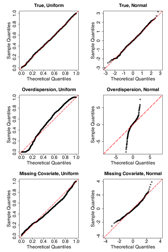
Figure 18: QQ plots of the proposed residuals under the uniform and normal scales.

B.1 Unraveling QQ Plots

When the model is correctly specified, our residuals should follow a uniform distribution. To construct QQ plots, one can plot the residuals against the quantiles of a uniform distribution. To understand the shape of the QQ plots of the proposed residuals, here we reproduce their patterns in a heuristic manner. We define the unobservable auxiliary residuals

$$\hat{r}_{M0}(Y_{i}|\mathbf{X}_{i})={G}_{M0}\left(\hat{F}_{M}(Y_{i}|\mathbf{X}_{i})\right),i=1,\ldots,n,$$

where ${G}_{M0}=\mathrm{E}_{\mathbf{X}}\left[F\left(\left.F_{M}^{(-1)}(s|\mathbf{X})\right|\mathbf{X}\right)\right]$ is the underlying distribution of ${F}_{M}(Y|\mathbf{X})$. The auxiliary residuals follow a uniform distribution. Since ${G}_{M0}$ is a monotone function, and $\hat{G}_{Mi}$ converges to $\mathrm{E}_{\mathbf{X}}\left[F_{M}\left(\left.F^{(-1)}_{M}(s|\mathbf{X})\right|\mathbf{X}\right)\right]$, which is also a monotone function, the rank of $\hat{r}(Y_{i}|\mathbf{X}_{i})$ among the proposed residuals is approximately same as the rank of $\hat{r}_{M0}(Y_{i}|\mathbf{X}_{i})$ among the auxiliary residuals. Therefore, the QQ plot of $\hat{r}(Y_{i}|\mathbf{X}_{i}),i=1,\ldots,n$ could, in theory, be approximated by plotting

$$\hat{r}(Y_{i}|\mathbf{X}_{i})\text{ against }\hat{r}_{M0}(Y_{i}|\mathbf{X}_{i}),i=1,\ldots,n.$$

The shape of the QQ plot of proposed residuals is thus determined by the relationship between $\hat{G}_{Mi}$ and $G_{M0}$. Furthermore, this relationship is preponderantly determined by the distinction between $\hat{F}_{M}$ and $F$, averaging over covariates. Therefore, if the QQ plot is above the diagonal, it implies that $\hat{F}_{M}(k)>F(k)$ on average, and vice versa.

This property of the proposed residuals can help identify certain causes of misspecification. In particular, the behavior in the lower tail displays the comparison between $\hat{F}_{M}(k)$ and $F(k)$ for a small $k$. Conversely, the behavior in the upper tail reflects the contrast between $\hat{F}_{M}(k)$ and $F(k)$ for a large $k$.

Acknoledgements

I thank Dr. James Hodges and the anonymous reviewers for their helpful comments. I gratefully acknowledge funding of the National Science Foundation (DMS-2210712).

Supplementary Material

Supplementary material:

The supplementary material includes additional simulation results and proofs of the theoretical results in Sections 4 and 2.4. (.pdf file)

R code and package:

The R code for simulation and data analysis. The proposed methodology is implemented in the assessor package. See the README contained in the zip file for more details. (code202312.zip, zip file)

References

- Anscombe (1953) Anscombe, F. (1953). Contribution to the discussion of h. hotelling’s paper. JR Stat. Soc B 15, 229–230.
- Ben and Yohai (2004) Ben, M. G. and V. J. Yohai (2004). Quantile–quantile plot for deviance residuals in the generalized linear model. Journal of Computational and Graphical Statistics 13(1), 36–47.
- Comizzoli et al. (1990) Comizzoli, R. B., J. M. Landwehr, and J. D. Sinclair (1990). Robust materials and processes: Key to reliability. AT&T Technical Journal 69(6), 113–128.
- Cook and Weisberg (1982) Cook, R. D. and S. Weisberg (1982). Residuals and influence in regression. New York: Chapman and Hall.
- Cook and Weisberg (1999) Cook, R. D. and S. Weisberg (1999). Graphs in statistical analysis: is the medium the message? The American Statistician 53(1), 29–37.
- Cordeiro and Simas (2009) Cordeiro, G. M. and A. B. Simas (2009). The distribution of pearson residuals in generalized linear models. Computational statistics & data analysis 53(9), 3397–3411.
- Cox and Snell (1968) Cox, D. R. and E. J. Snell (1968). A general definition of residuals. Journal of the Royal Statistical Society. Series B (Methodological), 248–275.
- Davison et al. (1989) Davison, A., Gigli, and A (1989). Deviance residuals and normal scores plots. Biometrika 76(2), 211–221.
- Dunn and Smyth (1996) Dunn, P. K. and G. K. Smyth (1996). Randomized quantile residuals. Journal of Computational and Graphical Statistics 5(3), 236–244.
- Faraway (2016) Faraway, J. J. (2016). Extending the linear model with R: generalized linear, mixed effects and nonparametric regression models. Chapman and Hall/CRC.
- Frees et al. (2011) Frees, E. W., G. Meyers, and A. D. Cummings (2011). Summarizing insurance scores using a gini index. Journal of the American Statistical Association 106(495), 1085–1098.
- Gan et al. (1991) Gan, F., K. J. Koehler, and J. C. Thompson (1991). Probability plots and distribution curves for assessing the fit of probability models. The American Statistician 45(1), 14–21.
- Goldman et al. (2001) Goldman, D. P., J. Bhattacharya, D. F. McCaffrey, N. Duan, A. A. Leibowitz, G. F. Joyce, and S. C. Morton (2001). Effect of insurance on mortality in an hiv-positive population in care. Journal of the American Statistical Association 96(455), 883–894.
- Hand and Henley (1997) Hand, D. J. and W. E. Henley (1997). Statistical classification methods in consumer credit scoring: a review. Journal of the Royal Statistical Society: Series A (Statistics in Society) 160(3), 523–541.
- Hosmer et al. (1997) Hosmer, D. W., T. Hosmer, S. Le Cessie, and S. Lemeshow (1997). A comparison of goodness-of-fit tests for the logistic regression model. Statistics in medicine 16(9), 965–980.
- Hosmer and Lemeshow (1980) Hosmer, D. W. and S. Lemeshow (1980). Goodness of fit tests for the multiple logistic regression model. Communications in statistics-Theory and Methods 9(10), 1043–1069.
- Landwehr et al. (1984) Landwehr, J. M., D. Pregibon, and A. C. Shoemaker (1984). Graphical methods for assessing logistic regression models. Journal of the American Statistical Association 79(385), 61–71.
- Lee et al. (2001) Lee, A. H., K. Wang, and K. K. Yau (2001). Analysis of zero-inflated poisson data incorporating extent of exposure. Biometrical Journal 43(8), 963–975.
- Li and Shepherd (2012) Li, C. and B. E. Shepherd (2012). A new residual for ordinal outcomes. Biometrika 99(2), 473–480.
- Liu et al. (2021) Liu, D., S. Li, Y. Yu, and I. Moustaki (2021). Assessing partial association between ordinal variables: quantification, visualization, and hypothesis testing. Journal of the American Statistical Association 116(534), 955–968.
- Liu and Zhang (2018) Liu, D. and H. Zhang (2018). Residuals and diagnostics for ordinal regression models: a surrogate approach. Journal of the American Statistical Association 113(522), 845–854.
- Miller et al. (1991) Miller, M. E., S. L. Hui, and W. M. Tierney (1991). Validation techniques for logistic regression models. Statistics in medicine 10(8), 1213–1226.
- Nattino et al. (2020) Nattino, G., M. L. Pennell, and S. Lemeshow (2020). Assessing the goodness of fit of logistic regression models in large samples: A modification of the hosmer-lemeshow test. Biometrics 76(2), 549–560.
- Pierce and Schafer (1986) Pierce, D. A. and D. W. Schafer (1986). Residuals in generalized linear models. Journal of the American Statistical Association 81(396), 977–986.
- Pregibon (1981) Pregibon, D. (1981). Logistic regression diagnostics. The annals of statistics 9(4), 705–724.
- Rosenman et al. (1975) Rosenman, R. H., R. J. Brand, C. D. Jenkins, M. Friedman, R. Straus, and M. Wurm (1975). Coronary heart disease in the western collaborative group study: Final follow-up experience of 8 1/2 years. Jama 233(8), 872–877.
- Shepherd et al. (2016) Shepherd, B. E., C. Li, and Q. Liu (2016). Probability-scale residuals for continuous, discrete, and censored data. Canadian Journal of Statistics 44(4), 463–479.
- Shi and Valdez (2014) Shi, P. and E. A. Valdez (2014). Multivariate negative binomial models for insurance claim counts. Insurance: Mathematics and Economics 55, 18–29.
- Su and Wei (1991) Su, J. Q. and L. Wei (1991). A lack-of-fit test for the mean function in a generalized linear model. Journal of the American Statistical Association 86(414), 420–426.
- Yang (2021) Yang, L. (2021). Assessment of regression models with discrete outcomes using quasi-empirical residual distribution functions. Journal of Computational and Graphical Statistics 30(4), 1019–1035.