Can transformers learn the greatest common divisor?

Abstract

I investigate the capability of small transformers to compute the greatest common divisor (GCD) of two positive integers. When the training distribution and the representation base are carefully chosen, models achieve $98\%$ accuracy and correctly predict $91$ of the $100$ first GCD. Model predictions are deterministic and fully interpretable. During training, the models learn to cluster input pairs with the same GCD, and classify them by their divisors. Basic models, trained from uniform operands encoded on small bases, only compute a handful of GCD (up to $38$ out of $100$): the products of divisors of the base. Longer training and larger bases allow some models to “grok” small prime GCD. Training from log-uniform operands boosts performance to $73$ correct GCD, and balancing the training distribution of GCD, from inverse square to log-uniform, to $91$ GCD. Training models from a uniform distribution of GCD breaks the deterministic model behavior.

1 Introduction

Transformers [30] have been successfully applied to many problems of symbolic [14, 3, 27] and numerical mathematics [2]. Yet, they struggle with basic arithmetic [15, 19]. Large transformers can memorize addition and multiplication tables for small integers (with $3$ or $4$ digits), but they fail to scale to larger operands. Recent fine-tuning techniques, such as scratchpad [20], chain-of-thought [31] or algorithmic prompting [34], allow large language models to generalize beyond their training range when performing addition or multiplication by a small prefactor (e.g. $3\times n$). But these techniques require bespoke training data, only apply to large pre-trained models, and struggle on complex tasks [8]. Interestingly, approximate arithmetic on floating point numbers proves easier to learn. Transformers can learn basic linear algebra [2], perform symbolic regression [6] and learn advanced computations such as eigen-decomposition [4] or finding the roots of polynomials [5].

There is, of course, little practical interest in replacing existing arithmetic algorithms, which are efficient and reliable, by transformer-based models. Nevertheless, investigating and better understanding the capabilities and limitations of transformers in elementary mathematics is an important line of research. As transformers are increasingly considered for scientific research [7, 23, 25], any limitation in their mathematical abilities will restrict their applicability to mathematics and science. Such limitations have already been postulated [19, 32], and even sometimes demonstrated [26].

This paper focuses on computing the greatest common divisor (GCD) of two positive integers , a key operation for arithmetic on rational numbers, and a common fixture of number theory. Initial experiments with rational arithmetic (Appendix A) indicate that transformers have no difficulty learning to compare fractions. Given four positive integers $a$, $b$, $c$ and $d$, a one-layer transformer can predict whether $\frac{a}{b}<\frac{c}{d}$ with $99.9\%$ accuracy. Transformers can also learn integer division, i.e. calculate $\lfloor\frac{a}{b}\rfloor$ (albeit with lower accuracy), but they cannot learn to add two fractions, or even reduce one in its lowest terms. A likely explanation for these results is that the models fail to compute GCD, which are needed for fraction addition and simplification, but not for comparison and integer division. If such a limitation of transformers was confirmed, it would compromise their use for problems involving integers and fractions. Without GCD, very little arithmetic on rational numbers is possible.

In this work, I investigate how 4-layer sequence-to-sequence transformers learn to compute the GCD of two positive integers in a range ($1$ to $10^{6}$), and make the following contributions:

1. Transformers trained on uniform random operands can achieve $95\%$ accuracy when predicting GCD, provided the base $B$ used to represent integers is carefully chosen. In other bases, it can be as low as $61\%$. These models leverage representation shortcuts to learn divisibility rules, and predict up to 38 (and as low as 1) GCD under $100$.

2. Model predictions are deterministic and fully interpretable. For any two integers with GCD $k$, the model always predicts the largest product of primes divisors of $B$ dividing $k$.

3. Models using large composite bases sometimes exhibit a phenomenon related to grokking [22], which allows them to learn multiples of small primes not dividing $B$.

4. Training models from log-uniform operands significantly improves performance, by providing the model with many simple instances. 73 GCD are correctly predicted.

5. Balancing the training set distribution of GCD, from inverse square to log-uniform, brings an additional boost to performance: 91 GCD are correctly predicted.

6. An unbalanced training distribution of outcomes is needed. Without it, model predictions are no longer deterministic (but some models can still learn $95$ GCD out of $100$).

Related work

Neural networks for arithmetic were proposed since the 1990s [28], and recurrent models (RNN, LSTM and related models) since 2015 [12, 33, 11]. Most recent research focuses on fine-tuning large pre-trained transformers on various arithmetic tasks, in order to solve math word problems [17, 9]. See Lee [15] for a summary of current capabilities and techniques. Neural Arithmetic Logical Units were introduced by Trask [29] as an alternative architecture for arithmetic. They learn exact computations, which generalize to any input, by constraining the weights of a linear network to be close to $0$, $1$ or $-1$ at the end of training. See Mistry [18] for a recent overview.

Several authors have noted the difficulty of training transformers on certain arithmetic tasks. Saxton [24] benchmarks many mathematical tasks, and observes that number theoretic operations, such as factorization, are hard. Palamas [21] further investigates the hardness of modular arithmetic. Dziri [8] notes the difficulty of extending the promising results obtained by transformers on the four operations [15] to complex mathematical algorithms (e.g. Euclid’s algorithm for the GCD).

The importance of number representation was discussed by Nogueira [19] in the case of arithmetic, and Charton [2] for linear algebra. Grokking was described by Power [22] for integer arithmetic. Liu [16] proposes interpretations and metrics to characterize grokking. Gromov [10] provides an insightful analysis of grokking in feed-forward networks trained to perform modular arithmetic.

2 Experimental settings

Through this work, GCD calculations are set up as a supervised translation task. Pairs of problems and solutions, $((a,b),\text{gcd}(a,b))$, with $a,b\in\mathbb{N}^{*}$, are randomly generated. Problems and solutions are encoded into sequences of tokens, and a sequence-to-sequence transformer [30] is trained to translate the problem into its solution, by minimizing the cross-entropy between model predictions and correct solutions. Integers are encoded as sequences of digits in base $B$, preceded by a sign token which also serves as a separator (Table 1). For instance, with $B=10$, the model learns to translate $(8,12)$, encoded as the sequence ‘+ 8 + 1 2’, into its GCD, $4$, encoded as ‘+ 4’.

The choice of $B$ is a trade-off. Small bases result in longer sequences that are harder to learn, but use a small vocabulary that is easier to memorize. Composite bases provide simple tests for divisibility. In base $10$, divisibility by $2$, $5$ and $10$ is decided by the rightmost token in the sequence.

Base	Encoded input	Encoded output
2	[+, 1, 0, 1, 0, 0, 0, 0, 0, +, 1, 1, 1, 1, 0, 0, 0]	[+, 1, 0, 1, 0, 0, 0]
6	[+, 4, 2, 4, +, 3, 2, 0]	[+, 1, 0, 4]
10	[+, 1, 6, 0, +, 1, 2, 0]	[+, 4, 0]
30	[+, 5, 10, +, 4, 0]	[+, 1, 10]

Table 1: Encoding gcd(160,120) = 40 in base 2, 6, 10 and 30

In all experiments, sequence-to-sequence transformers, with $4$ layers, $512$ dimensions and $8$ attention heads, are trained on batches of $256$ examples. The optimizer is Adam [13], with a constant learning rate of $10^{-5}$. All experiments are run on one NVIDIA V100 GPU with $32$ GB of memory.

Training examples are generated by uniformly sampling integers $a$ and $b$ between $1$ and $M=10^{6}$, and computing their GCD. After each epoch (300,000 examples), trained models are tested on sets of 100,000 random examples. New test data is generated after each epoch.The size of the problem space ($M^{2}=10^{12}$) guarantees minimal duplication between train and test set.

Model are tested on two sets. In the natural test set, input pairs $(a,b)$ are uniformly distributed, and the distribution of GCD, verifies $P(\text{gcd}(a,b)=k)=\frac{1}{k^{2}}$ [1], i.e. small GCD are more common. In the stratified test set, GCD are uniformly distributed between $1$ and $100$. It is generated as follows:

• Sample $k$, uniformly between $1$ and $100$.

• Sample $a$ and $b$, uniformly between $1$ and $\frac{M}{k}$, such that $\text{gcd}(a,b)=1$ (using rejection sampling, since $P(\text{gcd}(a,b)=1)=0.608$).

• Add $(ka,kb)$ to the stratified test set.

For every $1\leq k\leq 100$, the stratified test set contains about $1000$ examples $(a,b)$, such that $\text{gcd}(a,b)=k$. These two test sets are used in all experiments, for all training distributions, and provide two measures of accuracy. Model accuracy, measured on the natural set, is the probability that the GCD of two random integers from $1$ to $M$ is correctly predicted. Model accuracy on the stratified test set is the number of GCD correctly predicted between $1$ and $100$.

3 Learning greatest common divisors

In this section, models are trained on pairs of integers uniformly sampled between $1$ and $10^{6}$, and encoded in $20$ bases, ranging from $2$ to $1024$. Accuracy (measured on the natural test set) is high for large composite bases: up to $96.8\%$ for base $420$, and $94.7\%$ for base $30$. On the other hand, it drops to $61.3\%$ for base $31$ and $84.7\%$ for base $10$ (Table 2).

Base	2	3	4	5	6	7	10	11	12	15
Accuracy	81.6	68.9	81.4	64.0	91.5	62.5	84.7	61.8	91.5	71.7
Base	30	31	60	100	210	211	420	997	1000	1024
Accuracy	94.7	61.3	95.0	84.7	95.5	61.3	96.8	61.3	84.7	81.5

Table 2: Accuracy as a function of encoding base. Best of three models.

Learning is very fast: for base $30$, models achieve $90\%$ accuracy after $2$ epochs (600,000 examples), and $93\%$ after $6$. Model size has little impact on performance (Tables 13 and 14 in Appendix B). For base $30$, $1$-layer transformers with $32$ dimensions (less than 300,000 trainable parameters), achieve $93.3\%$ accuracy. $24$-layer models with $1024$ dimensions ($714$ million parameters) achieve $93.4\%$. For base $31$, performance is unchanged, at $61\%$, across all model sizes.

The influence of integer representation (base $B$) on model performance was observed in prior works [19, 2]. Still, the large variations in model accuracy for different bases are puzzling. Table 3 summarizes model predictions for bases $2$ and $10$, for GCD up to $36$ (Tables 18 and 19 in Appendix D.2 cover GCD up to $100$ and bases $2$, $4$, $10$, $30$, $31$ and $420$). For each GCD, it indicates the most frequent model prediction (Pred), and it frequency in the stratified test set ($\%$). All frequencies are close to $100\%$: the model predicts a unique value for every test pair with GCD $k$. This suggests that the model can tell that two pairs have the same GCD. Also, products of divisors of the base are always correctly predicted. In fact, all model predictions can be summarized by the three rules:

	Base 2		Base 10			Base 2		Base 10			Base 2		Base 10
GCD	Pred	%	Pred	%	GCD	Pred	%	Pred	%	GCD	Pred	%	Pred	%
1	1	100	1	100	13	1	100	1	100	25	1	100	25	100
2	2	100	2	100	14	2	100	2	100	26	2	100	2	100
3	1	100	1	100	15	1	100	5	100	27	1	100	1	100
4	4	100	4	100	16	16	100	16	99.7	28	4	100	4	100
5	1	100	5	100	17	1	100	1	100	29	1	100	1	100
6	2	100	2	100	18	2	100	2	100	30	2	100	10	100
7	1	100	1	100	19	1	100	1	100	31	1	100	1	100
8	8	100	8	100	20	4	100	20	100	32	32	99.9	16	99.9
9	1	100	1	100	21	1	100	1	100	33	1	100	1	100
10	2	100	10	100	22	2	100	2	100	34	2	100	2	100
11	1	100	1	100	23	1	100	1	100	35	1	100	5	100
12	4	100	4	100	24	8	100	8	100	36	4	100	4	100

Table 3: Model predictions and their frequencies, for GCD 1 to 36. Correct predictions in bold face.

1. Predictions are deterministic. In over $99.9\%$ of test cases, for any pair of integers with GCD $k$, the model predicts a unique value, $f(k)$, correct when $f(k)=k$.

2. Correct predictions are products of primes dividing B. For base $2$, they are $1$, $2$, $4$, $8$, $16$, $32$ and $64$. For base $31$, $1$ and $31$. For base $10$, all products of elements from $\{1,2,4,8,16\}$ and $\{1,5,25\}$. For base $30$, all products of $\{1,2,4,8,\}$, $\{1,3,9,27\}$. and $\{1,5,25\}$.

3. f(k) is the largest correct prediction that divides k. For instance, $f(15)=5$ for base $10$. $f(6)=2$ and $f(12)=4$ for bases $2$, $4$ and $10$, but $f(6)=6$ and $f(12)=12$ for base $30$.

For prime bases, model predictions and the three rules suggest that the model learns to count the rightmost zeros in its input. The representation of an integer divisible by $B^{n}$ ends with $n$ zeros. By counting the rightmost zeros, $z_{a}$ and $z_{b}$, of its operands, taking the minimum $\text{min}(z_{a},z_{b})=z$ and predicting $B^{z}$, a model accounts for all observed predictions, and satisfies the three rules. For instance, in base $2$, the model will correctly predict the GCD of $8=1000_{2}$ and $12=1100_{2}$ ($3$ and $2$ rightmost zeros), as $2^{2}=4$. On the other hand, it will wrongly predict the GCD of $7=111_{2}$ and $14=1110_{2}$ as $1$. For composite bases, divisibility by divisors of $B$ is also reflected in the rightmost digits of numbers. Once models learn these divisibility rules, their predictions satisfy the three rules.

The three rules also explain the variations in accuracy in Table 2. The probability that two random numbers have GCD $k$ is $\frac{6}{\pi^{2}k^{2}}$ [1]. Assuming that all products of prime divisors of $B$ are correctly predicted, we can compute a theoretical model accuracy for any base. If $B$ = $p^{k}$, with $p$ prime, the maximal accuracy is

$$\mathcal{A}(p^{k})=\mathcal{A}(p)=\frac{6}{\pi^{2}}\sum_{i=0}^{\infty}{\frac{1}{p^{2i}}}=\frac{6}{\pi^{2}}\frac{p^{2}}{p^{2}-1},$$

if $B=p^{k}q^{l}$, $\mathcal{A}(B)=1-\frac{\pi^{2}}{6}(1-\mathcal{A}(p))(1-\mathcal{A}(q)),$

if $B=p^{k}q^{l}r^{m}$, $\mathcal{A}(B)=1-\frac{\pi^{4}}{36}(1-\mathcal{A}(p))(1-\mathcal{A}(q))(1-\mathcal{A}(r))$, and so on.

Table 4 compares theoretical accuracies with empirical observations. Best model performances may be higher than theory, because of sampling errors in the test set, or lower than theory when some powers of prime divisors of $B$ have not been learned.

Base	2	3	4	5	6	7	10	11	12	15
Best model	81.6	68.9	81.4	64.0	91.5	62.5	84.7	61.8	91.5	71.7
Theory	81.1	68.4	81.1	63.3	90.2	62.1	88.6	61.3	90.2	80.3
Correct GCD	7	5	7	3	19	3	13	2	19	9
Base	30	31	60	100	210	211	420	997	1000	1024
Best model	94.7	61.3	95.0	84.7	95.5	61.3	96.8	61.3	84.7	81.5
Theory	94.1	60.9	94.1	88.6	96.3	60.8	96.3	60.8	88.6	81.1
Correct GCD	27	2	28	13	32	1	38	1	14	7

Table 4: Best model accuracy, theoretical accuracy and number of GCD<100 correctly predicted.

This analysis demonstrates a shortcoming of naive benchmarks. Accuracies measured on the natural test set, which over-represents small GCD, are very misleading. Base $12$ models achieve $91\%$ accuracy, yet only predict $19$ of the first $100$ GCD. Table 4 reports the number of correctly predicted GCD (accuracy on the stratified test set), which will be our main performance metric from now on.

Even our best models have not learned to compute GCD in the general case. Instead, they leverage representation shortcuts to predict a few easy but common instances. On the other hand, all models have learned to classify pairs of integers according to their GCD: for any pair of integers with GCD $k$, they always make the same prediction $f(k)$. This is an important result and a significant achievement.

Learning GCD one prime power at a time. Learning curves for the number of correct GCD (accuracy on the stratified test set), for base $30$, $21$ and $420$ (Figure 2) exhibit a step-like shape, which suggests that GCD are learned in batches, over small periods of training time. The learning curve for base $30$ has four steps. First, the model predicts $\{1,2,4\}$, $\{1,3,9\}$, $\{1,5\}$ and their products: $17$ correct GCD under $100$. Around epoch $50$, the model learns to predict $25$ and the three associated multiples: $50$, $75$ and $100$ ($21$ GCD). At epoch $220$, it learns $8$, and the multiples $24$, $40$ and $72$, and at epoch $660$, it learns $27$ and $54$, for a grand total of $27$ correct GCD under $100$.

For base $210$, the model first learns the $20$ products $\{1,2,4\}$, $\{1,3\}$, $\{1,5\}$ and $\{1,7\}$. At epoch $30$, it learns to predict $9$ and the associated multiples $18$, $36$, $45$, $63$ and $90$. $25$ and three more multiples are learned at epoch $400$, and $49$ and $98$ at epoch $500$, for a total of $32$ correct GCD. The three rules hold throughout training: all GCD $k$ are predicted as the largest predicted GCD dividing $k$.

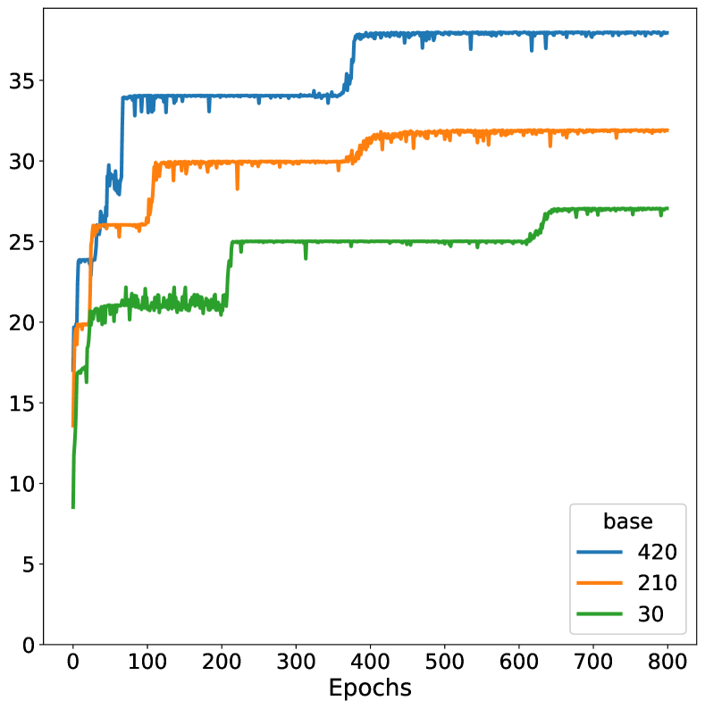
Figure 1: Correct GCD vs training time. Natural ($\frac{1}{k^{2}}$) distribution of GCD.

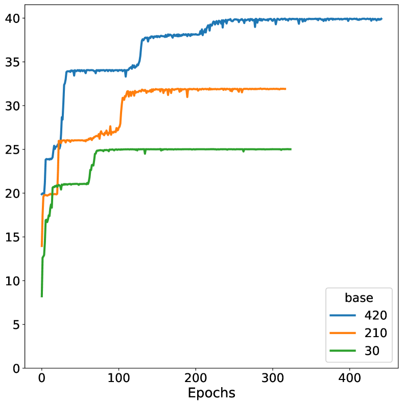
Figure 2: Correct GCD vs training time. 5% uniform, 95% natural GCD.

Accelerating learning by balancing the distribution of GCD. While products of small primes are learned in a few epochs, large powers of primes require a lot of training: the length of flat steps in the learning curves increases over time. This is due to the distribution of GCD in the training set, which contains $10$ times more examples with GCD $1$ than GCD $10$, and $1000$ times more than GCD $32$. This can be mitigated by adding a small proportion ($5\%$) of uniformly sampled GCD to the training set, using the same generation technique as for the stratified test set. This adjustment increases the proportion of large GCD in the training set and has a major impact on learning speed (Figure 2). For base $30$, the model learns $25$ GCD in $30$ epochs, instead of $250$, and $27$ GCD in $175$ (vs $650$).

4 Large composite bases $B$ - grokking small primes

So far, the only GCD correctly predicted are product of primes divisors of the base. Non-divisors of $B$ are learned in a small number of cases, always involving large bases ($1000$ and $1024$), and after extensive training. In one experiment with base $1000$, the model correctly predicts $13$ GCD after $84$ epochs: all the products of $\{1,2,4,8,16\}$ and $\{1,5,25\}$. For the next $100$ epochs, training and test losses are flat, and it seems that the model is not learning anymore. Yet, at epoch $188$, the model begins to predict GCD $3$, with accuracy $0.2\%$ at epoch $188$, and $93\%$ at epoch $193$ (despite only seeing 100,000 examples with GCD $3$ during these $5$ epochs). Multiples of $3$ are then learned, and by epoch $220$, the model predicts $22$ GCD: products of $\{1,2,4,8,16\}$, $\{1,5,25\}$ and $\{1,3\}$.

This phenomenon is related to grokking, first described by Power [22] for modular arithmetic. Table 5 presents model predictions for base $1000$, which continue to respect rules R1 and R3. In fact, we can update the three rules into the three rules with grokking:

1. Prediction is deterministic. All pairs with the same GCD are predicted the same, as $f(k)$.

2. Correct predictions are products of primes divisors of B, and small primes. Small primes are learned roughly in order, as grokking sets in.

3. f(k) is the largest correct prediction that divides k.

GCD	Prediction	GCD	Prediction	GCD	Prediction	GCD	Prediction	GCD	Prediction
1	1	11	1	21	3	31	1	41	1
2	2	12	12	22	2	32	16/ 32	42	6
3	3	13	1	23	1	33	3	43	1
4	4	14	2	24	24	34	2	44	4
5	5	15	15	25	25	35	5	45	15
6	6	16	16	26	2	36	12	46	2
7	1	17	1	27	3	37	1	47	1
8	8	18	6	28	4	38	2	48	48
9	3	19	1	29	1	39	3	49	1
10	10	20	20	30	30	40	40	50	50

Table 5: Grokked model predictions. $B=1000$, after $220$ epochs. $32$ is being learned.

Grokking almost never happens in our initial experiments, but it is common in large bases when models are trained long enough. Table 6 presents results for models trained on $16$ large bases, most of them composite, for up to $1300$ epochs ($390$ million examples). Grokking happens in all models, but takes a long time to happen. For instance, for bases $625$ and $4000$, products of prime divisors of $B$ are learned in $5$ and $15$ epochs, but grokking only begins after $600$ epochs. In all experiments, primes and powers of primes are grokked in order, with a few exceptions (e.g. in two different models with base $2401$, $2$ and $3$ are grokked in different order).

Base		GCD predicted	Divisors predicted	Non-divisors (epoch learned)
$625=5^{4}$		6	{1,5,25}	2 (634)
$2017$		4	{1}	2 (142), 3 (392)
$2021=43.47$		10	{1,43}, {1,47}	2 (125), 3 (228)
$2023=7.17^{2}$		16	{1,7}, {1,17}	3 (101), 2 (205), 4 (599)
$2025=3^{4}.5^{2}$		28	{1,3, 9, 27, 81}, {1,5,25}	2 (217), 4 (493), 8 (832)
$2187=3^{7}$		20	{1,3,9,27,81}	2 (86), 4 (315) , 5 (650)
$2197=13^{3}$		11	{1,13}	2 (62), 3 (170), 4 (799)
$2209=47^{2}$		8	{1,47}	2 (111), 3 (260), 9 (937)
$2401=7^{4}$		10	{1,7,49}	2 (39), 3 (346)
$2401=7^{4}$		14	{1,7,49}	3 (117), 2 (399), 4 (642)
$2744=2^{3}.7^{3}$		30	{1,2,4,8,16,32}, {1,7,49}	3 (543), 5 (1315)
$3125=5^{5}$		16	{1,5,25}	2 (46), 3 (130), 4 (556)
$3375=3^{3}.5^{3}$		23	{1,3,9,27}, {1,5,25}	2 (236), 4 (319)
$4000=2^{5}.5^{3}$		24	{1,2, 4,8,16,32}, {1, 5, 25 }	3 (599)
$4913=17^{3}$		17	{1,17}	2 (54), 3 (138), 4 (648), 5 (873)
$5000=2^{3}.5^{4}$		28	{1,2,4,8,16,32}, {1,5,25}	3 (205), 9 (886)
$10000=2^{4}.5^{4}$		22	{1,2,4,8,16}, {1,5,25}	3 (211)

Table 6: Predicted gcd, divisors and non-divisors of ${\bf B}$. Best model of 3. For non-divisors, the epoch learned is the first epoch where model achieves $90\%$ accuracy for this gcd.

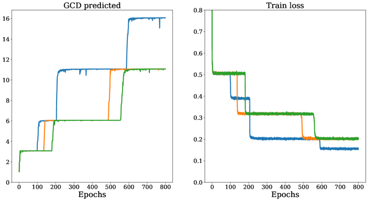
Figure 6: Learning curves for base B=2023. 3 different model initializations.

Learning curves for base $2023$ are presented in Figure 6 of Appendix D.1. Learning proceeds in steps: long periods of stagnation followed by sudden drops in the loss and rises in accuracy, as new GCD and their multiples are learned. Whereas all models grok the same GCD in the same order, the number of epochs needed varies a lot with model initialization (from $200$ to $600$ for base $2023$). Because it helps models learn small primes, grokking provides a large boosts in model accuracy. For base $2023$, accuracy increases from $63\%$ to $91\%$ as $2$, $3$ and $4$ are learned. On the other hand, in all experiments, the number of correct GCD remains under $30$ after grokking.

Balancing outcomes. Grokking requires a lot of examples. Adding a small proportion of uniformly distributed GCD to the training set, as in section 3, brings no clear benefit (Table 17 in Appendix D.2). Instead, I change the training distribution of GCD to log-uniform, so that it scale as $\frac{1}{k}$ instead of $\frac{1}{k^{2}}$. This can be achieved by sampling operands as follows:

• Sample $k$ between $1$ and $100$, with probability $P(k)=\frac{1}{Ck}$, with $C=\sum_{i=1}^{100}{\frac{1}{i}}$.

• Sample two integers $a$ and $b$, uniformly from $1$ to $M/k$, such that $\text{gcd}(a,b)=1$.

• Add $(ak,bk)$ to the training set.

	Natural	Log-uniform outcomes			Natural	Log-uniform outcomes
Base	# GCD	# GCD	Additional divisors	Base	# GCD	# GCD	Additional divisors
2	7	7	-	997	1	1	-
3	5	5	-	1000	22	31	9, 32, 64
4	7	7	-	2017	4	6	9
5	3	3	-	2021	10	10	-
6	19	20	64	2023	16	11	-
7	3	3	-	2025	28	28	-
10	13	14	32	2187	20	20	-
11	2	2	-	2197	11	11	-
12	19	20	81	2209	8	8	-
15	9	10	81	2401	14	16	5
30	25	36	16, 29, 31	2744	29	21	-
31	2	2	-	3125	16	16	-
60	28	33	27, 32, 64	3375	23	21	-
100	13	15	32, 64	4000	25	31	9, 64
210	32	32	-	4913	17	9	-
211	1	18	2,3,4,5,7	5000	28	30	64
420	38	47	13, 49	10000	22	40	7, 9, 32
625	6	9	4	10000	22	62	7, 9, 13, 27, 32, 64

Table 7: Log-uniform outcome distributions. Best model of 3, trained for 700 epochs. Non-divisors in bold.

For $9$ bases out of $35$, a log-uniform distribution of GCD in the training set helps models learn non-divisors of $B$ (Table 7). For $B=211$, primes up to $7$ are learned. For $B=10000$, $7$, $9$, $13$ and $27$ are learned, bringing the number of correct GCD to $62$, our best result so far. For $B=30$, a counter-intuitive situation prevails: instead of small primes, the model learns $B-1$ and $B+1$.

5 Learning from log-uniform operands

In all experiments so far, the input pairs $(a,b)$ in the training set are uniformly sampled between $1$ and $M=10^{6}$. As a result, models are mostly trained from examples with large operands. $90\%$ of operands are $6$-digit integers, and small examples (e.g. $\text{gcd}(6,9)$) are almost absent from the training set. In contrast, when teaching arithmetic, we usually insist that examples with small operands must be learned, and sometimes memorized, before students can generalize to larger instances.

In this section, we sample input pairs in the training set from a log-uniform distribution, uniformly sampling real numbers $x$ between $0$ and $\log M$, computing $e^{x}$ and rounding to the nearest integer. In this setting, the training set has as many $1$-digit operands as $6$-digit operands, and the number of $a$ scales as $\frac{1}{a}$. In $3\%$ of training examples, both operands are smaller than $10$, in $11\%$ both are smaller than $100$. This presents the model with many GCD of small integers that it can memorize, just like children rote learn multiplication and addition tables. This is different from curriculum learning: the training distribution does not change over time. Note that log-uniform sampling only applies to the training set (test sets are unchanged), and has no impact on the distribution of outcomes.

Base	Accuracy	Correct GCD	Base	Accuracy	GCD	Base	Accuracy	GCD
2	94.4	25	60	98.4	60	2025	99.0	70
3	96.5	36	100	98.4	60	2187	98.7	66
4	98.4	58	210	98.5	60	2197	98.8	68
5	97.0	42	211	96.9	41	2209	98.6	65
6	96.9	39	420	98.1	59	2401	99.1	73
7	96.8	40	625	98.2	57	2744	98.9	72
10	97.6	48	997	98.3	64	3125	98.6	65
11	97.4	43	1000	99.1	71	3375	98.8	67
12	98.2	55	1024	99.0	71	4000	98.7	66
15	97.8	52	2017	98.6	63	4913	98.2	57
30	98.2	56	2021	98.6	66	5000	98.6	64
31	97.2	44	2023	98.7	65	10000	98.0	56

Table 8: Accuracy and correct GCD (up to 100), log-uniform operands. Best of three models, trained for 1000 epochs (300M examples). All models are tested on 100,000 pairs, uniformly distributed between 1 and $10^{6}$.

Training from log-uniform operands greatly improves performance (Table 8). Accuracy for all bases is between $94$ and $99\%$, vs $61$ and $97\%$ with uniform operands. For base 2401, the number of correct GCD is 73, our best result so far. For base $10$, the number of correct GCD is $48$ (vs $13$). For base $1000$, it is $71$ (vs $22$ with grokking). As before, large bases perform best: for all models with $B\leq 420$, accuracy is higher than $98\%$, and more than $55$ GCD are correctly predicted.

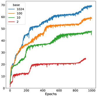
Figure 3: Learning curves, Log-uniform training set.

The learning process is the same as in previous experiments. Models first learn the products of small powers of primes dividing $B$, then small powers of prime non-divisors are “grokked”, in sequence. For base $2$, the best model predicts $25$ GCD: products of powers of $2$ up to $64$, $3$ and $5$. For base $10$, the best model predicts powers of $2$ up to $16$ and powers of $5$ up to $25$, as in previous experiments, but also $3$, $7$, $9$ and $11$. For base $100$, models learn $\{1,2,4,8,16\}$, $\{1,5,25\}$ and $3$, $7$, $9$, $11$, $13$ and $17$.

Learning curves retain their step-like shape (Figure 3), but they are noisy, and their steps are less steep. For base $2$, all small powers of $2$ are learned by epoch $25$, then $3$ by epoch $50$ and $5$ by epoch $300$. At epoch $925$, GCD $7$ is predicted with accuracy $40\%$. For base $10$, GCD $1,2,4$ and $5$ are learned as early as epoch $3$, $3$ and $8$ by epoch $25$, $7$ and $9$ by epoch $220$ and $11$ by epoch $750$.

For base $1024$ ($2401$ and $2844$), only $27$ GCD are incorrectly predicted (the three rules are respected):

• the $16$ primes from $29$ and $97$, all predicted as $1$,

• small multiples of these primes: products of $2$ and $29,31,37,41,43$ and $47$, predicted as $2$, and products of $3$ and $29$ and $31$, predicted as $3$,

• powers of small primes: $49=7^{2}$, predicted as $7$, and $81=3^{4}$, predicted as $27$.

• small multiples of these: $98=49*2$, predicted as $14$.

Overall, training from log-uniform operands improves model performance by accelerating the grokking process. After training, models have learned to predict all primes up to a certain value ($23$ for the best models), some of their small powers, and all associated products. This brings model accuracy on random pairs to $99\%$, and the number of correct GCD under $100$ to $73$. The three rules with grokking (G1 to G3) still apply. Models make deterministic predictions, and for a pair $(a,b)$ with GCD $k$, they predict a unique number $f(k)$: the largest correctly predicted GCD that divides $k$.

During training, rules G1 and G3 can be temporarily violated while the model learns a new factor. During a few epochs, model predictions will be split between the old and the new value (e.g. between $7$ and $49$ while the model learn $49$). This situation was rarely observed in previous experiments, when transitions were faster. They become common with log-uniform operands.

Base	Accuracy	Correct GCD	Base	Accuracy	GCD	Base	Accuracy	GCD
2	16.5	17	60	96.4	75	2025	97.9	91
3	93.7	51	100	97.1	78	2187	97.8	91
4	91.3	47	210	96.2	80	2197	97.6	90
5	92.2	58	211	95.3	67	2209	97.6	87
6	95.2	56	420	96.4	88	2401	97.8	89
7	93.0	63	625	96.0	80	2744	97.6	91
10	94.3	65	997	97.6	83	3125	97.7	91
11	94.5	57	1000	97.9	91	3375	97.6	91
12	95.0	70	1024	98.1	90	4000	97.3	90
15	95.4	62	2017	97.6	88	4913	97.1	88
30	95.8	72	2021	98.1	89	5000	97.1	89
31	94.4	64	2023	97.5	88	10000	95.2	88

Table 9: Accuracy and correct GCD, log-uniform operands and outcomes. Best model of 3.

Log-uniform outcomes. Balancing the distribution of outcomes in the training set to make it log-uniform (as in section 4), brings a large improvement in performance (Table 9). After $1000$ epochs, models with bases larger than $1000$ predict $87$ to $91$ GCD: all primes up to $53$ and all composite numbers up to $100$. These are our best results. For large bases, they can be improved by using an inverse square root distribution of outcomes (Table 15 in Appendix C.1). For small bases, log-uniform outcomes sometimes degrade performance. For base $2$, accuracy drops to $16.5\%$, as the model struggles to learn to predict GCD $1$, for lack of examples.

6 Learning from uniform outcomes

Log-uniform distributions of outcomes improve model performance by reducing the imbalance between small and large GCD in the training set. In this section, I push this idea further, and eliminate all imbalance by training models from a uniform distribution of outcomes and operands, using the same sampling procedure for the training set and the stratified test set (see Section 2).

Figure 4 presents test losses and accuracies for three models trained on uniform operands and outcomes, with $B=10$. Model accuracy seems to vary randomly during training, and the loss is not reduced. Yet, the number of correct GCD is stable, and increases in steps, from $10$ to $13$ and $17$ GCD, in line with the results from section 3 ($13$ GCD). Something is being learned, despite the flat loss.

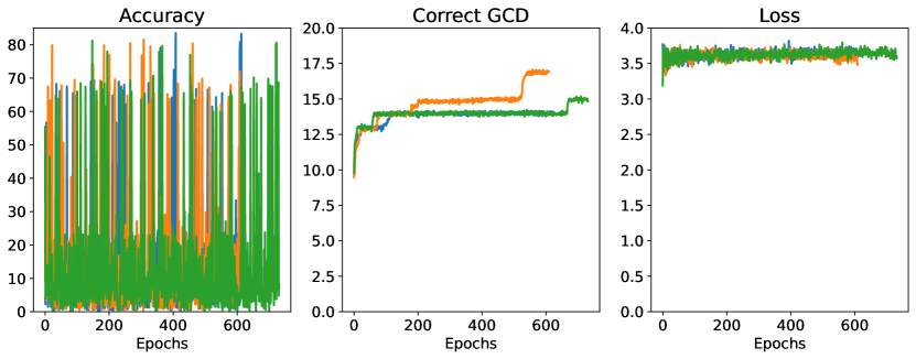
Figure 4: Learning curves for B=10. Uniform outcomes and operands. 3 different seeds.

At first glance, model predictions seem chaotic. At epoch 266, one model achieves $81\%$ accuracy, and predicts $14$ GCD: $1$, $2$, $5$, $8$, $20$, $32$, $40$, $44$, $48$, $50$, $64$, $75$, $80$ and $100$. One epoch later, accuracy is down to $6\%$, the model still predicts $14$ GCD: $4$, $8$, $10$, $16$, $40$, $50$, $55$, $60$, $64$, $66$, $75$, $80$, $95$ and $100$, but half of the correct GCD have changed! After another epoch, accuracy is $4\%$ and the model predicts $4$, $20$, $25$, $26$, $30$, $32$, $40$, $48$, $50$, $55$, $64$, $73$, $80$, $88$ and $100$.Again, half the GCD changed.

	Epoch 266		Epoch 267		Epoch 268		Epoch 269		Epoch 270		Epoch 580		Epoch 581
	Pred	%	Pred	%	Pred	%	Pred	%	Pred	%	Pred	%	Pred	%
1	1	100	19	54	73	100	7	100	13	100	1	98	77	99
2	2	100	66	100	26	100	62	100	66	100	22	93	22	99
3	1	100	19	52	73	100	7	100	13	100	1	99	77	99
4	44	91	4	100	4	100	44	100	4	100	4	100	4	100
5	5	100	55	100	55	100	55	100	5	100	5	100	5	100
6	2	100	66	100	26	200	62	100	66	100	22	93	22	99
7	1	100	19	62	73	100	7	100	13	100	1	99	77	99
8	8	99	8	100	88	100	8	100	8	100	88	100	88	99
9	1	100	19	53	73	100	7	100	13	100	1	99	77	99
10	70	70	10	100	30	99	70	100	70	100	30	100	70	100
11	1	100	19	57	73	100	7	100	13	100	1	98	77	99
12	44	91	4	100	4	100	44	100	4	100	4	100	18	22
13	1	100	19	55	73	100	7	100	13	100	1	98	77	99
14	2	100	66	100	26	100	62	100	66	100	22	92	22	99
15	5	100	55	100	55	100	55	100	5	100	5	100	5	100
16	48	97	16	84	48	99	48	99	16	98	48	98	48	78
17	1	100	19	54	73	100	7	100	13	100	1	99	77	100
18	2	100	66	100	26	100	62	100	66	100	22	93	22	99
19	1	100	19	53	73	100	7	100	13	100	1	99	77	99
20	20	100	60	100	20	98	20	100	20	53	20	100	20	100

Table 10: Prediction for base 10 - uniform operands and outcomes. Most common prediction for GCD 1 to 20, and frequency, for successive epochs. Correct predictions are in bold

Further analysis reveal regular patterns. Table 10 presents the most common model predictions for all GCD up to $20$, and their frequencies. First, note that model predictions remain deterministic: most predictions have a frequency close to $100\%$ (i.e. all pairs with this GCD are predicted the same), with the exception of epoch $267$, when predictions for $1$, $3$, $7$, $11$, $13$, $17$ and $19$ are equally split between $11$ and $19$. Second, groups of GCD are predicted the same. All elements in class $C_{1}=\{1,3,7,9,11,13,17,19\}$ are predicted as $1$ at epoch $266$, $19$ at epoch $267$, $73$ at epoch $268$, and os on. Similar patterns occur for classes $C_{2}=\{2,6,14,18\}$, $C_{4}=\{4,12\}$ and $C_{5}=\{5,15\}$.

These classes correspond to the multiples of $1$, $2$, $4$, and $5$, and would have been predicted as $1$, $2$, $4$, and $5$ by a base $10$ model following the three rules from section 3. In other words, the model classifies GCD exactly like a model trained on a natural distribution of outcomes, but its predictions for each class vary over time. Finally, note that model predictions for each class are elements of the class: elements of $C_{1}$ are predicted as $1$, $7$, $11$, $19$, elements of $C_{2}$ as $2$, $22$, $62$, $66$. In fact, all model predictions are accounted for by the three rules with uniform outcomes:

1. Predictions are mostly deterministic. At a given epoch, the model usually predicts a unique value $f(k)$ for a given GCD $k$. In rare cases, the model makes $2$ or $3$ predictions.

2. Classes of multiples of products of prime divisors of B are predicted the same. For base $10$, classes are $\{1,3,7,9,11,13,17,19\dots\}$, $\{2,6,14,18,22,26,34,38\dots\}$, $\{4,12,21,36,44,52,\dots\}$, $\{5,15,35,55\dots\}$ …

3. For each class, at every epoch, the (unique) model prediction is an element of the class. Predictions vary from one epoch to the next. However, the number of correctly predicted GCD is constant over time: it is the number of classes. It increases over time, as the model learns new multiples of primes divisors of $B$).

The three rules account for both the chaotic shape of the accuracy curve and the step-like shape of the number of correct GCD. Since $61\%$ of test examples in the natural test set (used to compute accuracy) have GCD $1$, accuracy jumps by $61\%$ every time class $C_{1}$ is predicted as $1$. On the other hand, rule U3 implies that the number of GCD is the number of classes, because at one given epoch, one of their elements is correctly predicted. This accounts for the step-shaped learning curve of correct GCD.

These results shed light on the learning process and the role of the distribution of outcomes. During training, all models, no matter their outcome distribution, learn to partition input pairs into classes. Each class is associated with a product $p$ of prime divisors of the base (e.g. $1$, $2$, $4$, $5$, $10$…), and contains all pairs $(a,b)$ with GCD $k$, such that $k$ is a multiple of $p$. Model predictions are the same for all pairs in the class. When the distribution of outcomes is unbalanced, the model learns to predict the most common element in the class, i.e. $f(p)=p$. When outcomes are uniformly distributed, one element of the class is selected, somewhat randomly, at every epoch.

For base 1000, learning curves (Figure 5) suggest that a similar situation occurs during the first $400$ epochs, with grokking, characterized by steep drops in the loss and increases in the number of correct GCD, happening between epochs 200 and 400. Then, accuracy rises steadily, as does the number of correct GCD, which reaches $95$ (out of $100$) after about $800$ epochs.

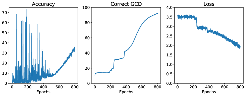
Figure 5: Learning curves for B=1000 - uniform operands and outcomes.

More precisely, by epoch 180, the model has learned to classify all examples into $14$ sets: multiples of $1$, $2$, $4$, $5$, $8$, $10$, $16$, $20$, $25$, $32$, $40$, $50$, $80$ and $100$. At each epoch, the model selects one element in each class, which is its unique prediction for all pairs of integers with GCD in the class.

Grokking set in around epoch $200$, and by epoch $220$, $5$ new classes have been learned: multiples of $11$ ($11$, $33$, $77$ and $99$), $22$, $44$, $55$ and $88$, created by “splitting away” the multiples of $11$ from the classes of multiples of $1$, $2$, $4$, $5$ and $8$. Note that small primes are not learned in increasing order anymore (in fact, the order varies with model initialization). This is another effect of uniform outcomes. By epoch 260, multiples of $3$ are learned and the model predicts $31$ different outcomes (splitting $12$ classes: $1$ to $32$). By epoch $400$, multiples of $7$ are learned, and $41$ GCD are predicted.

At that point, a new phenomenon sets in: model predictions are no longer deterministic. Until then, all pairs with the same GCD would be predicted the same at every epoch (or split between two values in rare cases). As grokking develops, more classes are created, and the frequencies of most common predictions for each class go down. By epoch 400, for pairs with GCD $1$, the model predicts $18$ different values, with frequencies ranging from $2\%$ to $13\%$ (Table 11).

GCD 1		GCD 2		GCD 3		GCD 4		GCD 5
Pred.	%	Pred	%	Pred	%	Pred	%	Pred	%
11	5	2	8	3 12	4	40	5	12
17	2	22	13	27	11	44	19	55	21
19	2	34	18	33	7	68	5	85	31
23	3	38	12	51	9	76	24	95	36
29	5	46	10	57	12	92	12
31	7	58	10	69	22
37	5	62	10	81	7
41	13	74	4	87	7
43	8	82	8	93	8
59	1	86	6	99	2
61	2
67	2
71	4
73	3
79	9
83	13
89	7
97	7

Table 11: Base 1000 - epoch 400 - predicted values and frequencies. Frequencies larger than 1%.

At this point, model predictions are neither deterministic nor interpretable, and the three rules are no longer respected. Classes have as many predictions as there are elements, and the model begins learning individual GCD, beginning with the largest ones (i.e. the smallest classes). By epoch 740, $95$ of the $100$ first GCD are correctly predicted, the worst performance being achieved on the smallest values (GCD $1$, $2$ and $3$, correctly predicted $43$, $74$ and $85\%$ of the time).

To summarize, for base $10$, the model only learns products of divisors of the base. Model predictions remain deterministic, but they change from an epoch to the next. For base $1000$, grokking sets in after $200$ epochs, and eventually causes models trained from uniform outcomes to stop making deterministic predictions. However, in the long run, they manage to learn the greatest common divisor, and predict $95$ GCD out of $100$.

7 Discussion

Can transformers learn the greatest common divisor? With enough examples, and appropriate adjustment of their training distribution, they can. Models leveraging large composite bases, and trained on log-uniform operands and outcomes predict more than $90$ of the $100$ first GCD. Models trained on uniform outcomes can predict $95$ GCD. However, the initial experiments from section 3 show the limits of naive, benchmark-based evaluations on arithmetic tasks: high accuracies can be achieved by models that only predict a handful of GCD.

The impact of the training distribution on model performance is an important finding, which may come as a surprise. Many authors observed that evaluating a model out of its training distribution has a negative impact on performance. In these experiments, all models are tested on uniformly distributed operands and outcomes, but the best results are achieved for models trained from log-uniform operands and outcomes. The existence of special training distributions, which allow for high performance across many test distributions, was observed for other numerical tasks [4].

The log-uniform distribution of operands strikes a balance between memorization and generalization. It provides the model with many easy examples that help learn general solutions. This prevents catastrophic forgetting, observed in curriculum learning when easy examples are presented at the beginning of training and progressively replaced by harder problems.

The log-uniform distribution of outcomes helps balance the training set by making large GCD more common, a classic recipe in machine learning. However, the counter-intuitive result is that making the GCD uniformly distributed in the training set, the best possible balancing act, actually hinders training by preventing the model from learning to predict small GCD. The results about log-uniform distributions probably apply to other arithmetic tasks, notably to the fine-tuning large language models on arithmetic tasks.

What are the models doing? Model predictability is probably the most striking feature of these experiments. It is often repeated that neural networks, and especially transformers, are incomprehensible black-boxes, that sometimes confabulate and often fail in unpredictable ways. In most experiments in this paper, model predictions are deterministic and can be fully explained by a small number of rules. These rules suggest that the model is learning GCD by applying a sieving algorithm.

Throughout training, the model learns divisibility rules, and uses them to partition its input pairs into classes of pairs with a common divisor. Early during training, this is limited to powers of divisors of the base, that the model can learn by counting the rightmost zeroes in the representation of integers. For base $2$, the model will partition its input into classes of pairs divisible by $1$, $2$, $4$, $8$. For composite bases, it will partition its input into classes of pairs divisible by products of primes dividing $B$. If training outcomes are unbalanced, each class will be predicted as its most common value, i.e. its minimum. At this point, all GCD corresponding to products of divisors of $B$ have been learned.

As training proceeds, new divisors are learned, in order if training outcomes are unbalanced. They are all prime because multiples of previous divisors were learned already, i.e. the model implements the sieve of Eratosthenes. When a new divisor $p$ is learned, new classes are created by splitting all existing classes between multiples and non-multiples of $p$. In base $2$, when the model learns divisibility by $3$, six new classes are created: multiples of $3$, $6$, $12$, $24$, $48$ and $96$. All GCD will eventually be learned, once all their prime factors are learned. Note that this algorithm relies on unbalanced outcomes in the training distribution: they guarantee that the model predicts the smallest element of every class, and that primes are learned in increasing order.

Is it really grokking? The characterization as grokking of the phenomenon observed in section 4 is not entirely correct. Power [22] defines grokking as “generalization far after overfitting.” In these experiments, training and test data are generated on the fly from a very large problem space. No overfitting can happen. As a result, the classical pattern of grokking, where train accuracy saturates for a long time before validation accuracy catches up, will not occur. The similarity with grokking lies in the sudden change in accuracy after a long stagnation of the training loss.

Appendix

Appendix A Rational arithmetic with transformers

In these experiments, transformers are trained to perform five arithmetic operations on positive rational numbers:

• comparison: given four positive integers $a,b,c$ and $d$, predict whether $\frac{a}{b}<\frac{c}{d}$.

• Integer division: given two integers $a$ and $b$, predict the integer $\lfloor\frac{a}{b}\rfloor$.

• Addition: given four integers $a,b,c$ and $d$, predict the sum $\frac{a}{b}+\frac{c}{d}$, in lowest terms.

• Multiplication: given four integers $a,b,c$ and $d$, predict the product $\frac{a}{b}\times\frac{c}{d}$, in lowest terms.

• Simplification: given two integers $a$ and $b$, predict the lowest term representation of $\frac{a}{b}$, i.e. $\frac{c}{d}$ with $c=\frac{a}{\text{gcd}(a,b)}$ and $d=\frac{b}{\text{gcd}(a,b)}$.

For the comparison, addition and multiplication tasks, all integers $a,b,c$ and $d$ are uniformly sampled between $1$ and $M$ (100,000 or 1,000,000).

For the simplification task, $3$ integers $m,n,p$ are uniformly sampled between $1$ and $M$, I let $a=\frac{pm}{\text{gcd}(m,n)}$ and $b=\frac{pn}{\text{gcd}(m,n)}$ and the model is tasked to predict $a$ and $b$.

For the integer division task, $3$ integers $m,n,p$ are uniformly sampled between $1$ and $M$, with $m<n$, I let $a=pn+m$ and $b=n$, and the model is tasked to predict $p=\lfloor\frac{a}{b}\rfloor$.

All integers are encoded as sequences of digits in base $B$ (see section 2. Sequence to sequence transformers with $4$ layers, $512$ dimensions and $8$ attention heads are trained to minimize a cross-entropy loss, using Adam with learning rate $10^{-4}$, inverse square root scheduling, linear warmup over $10,000$ optimization steps, and a batch size of $256$. After each epoch (300,000 examples), models are tested on 100,000 random examples.

Table 12 presents model accuracies for the five operations, for four bases ($10$, $30$, $31$ and $1000$), and $M=10^{5}$ and $=10^{6}$. All models are trained for more than $1000$ epochs. Comparison is learned to very high accuracy, and integer division to some extent. On the other hand, the three tasks involving GCD calculations (simplification, addition and multiplication) are not learned.

	Comparison		Integer division		Simplification		Addition		Multiplication
Base	M=$10^{5}$	M=$10^{6}$	M=$10^{5}$	M=$10^{6}$	M=$10^{5}$	M=$10^{6}$	M=$10^{5}$	M=$10^{6}$	M=$10^{5}$	M=$10^{6}$
10	100	100	21.2	2.4	0.14	0.02	0	0	0	0
30	99.9	100	14.2	2.2	0.21	0.02	0	0	0	0
31	99.9	100	14.3	2.4	0.02	0	0	0	0	0
1000	100	99.9	8.8	0.7	0.09	0.01	0	0	0	0

Table 12: Rational arithmetic with transformers. Accuracy of trained models Best of 3 models, trained for $1000$ to $1500$ epochs.

Appendix B Model scaling for the base experiments

Section 3 presents results for $4$-layer transformers with $512$ dimensions and $8$ attention heads. In this section, I experiment with very small models (down to $1$ layer and $32$ dimensions), and very large ones (up to $24$ layers and $1024$ dimensions). Note: Tables 13 and 14 indicate the number of trainable parameters in the models. These change with the encoding base (large vocabularies mean more parameters in the embedding layers). All parameter counts are for $B=10$.

Table 13 presents accuracies for models with one layer, $8$ attention heads, and $32$ to $512$ dimensions. These models have $3$ to $100$ times less parameters that the 4-layer baseline. Yet, there is no large change in trained model accuracy for $12$ different bases.

Table 14 presents results for models from $6$ to $24$ layers, symmetric (same number of layers in the encoder and decoder), or asymmetric (with a one-layer encoder or decoder). The dimensions are $512$, $640$, $768$ and $1024$ for $6$, $8$, $12$, and $24$ layers, and the dimension to attention head ratio is kept constant at $64$ (i.e.there are $8$, $10$, $12$ and $24$ attention heads respectively). Model size has no significant impact on accuracy.

	512 dimensions	256 dim.	128 dim.	64 dim.	32 dim.	4-layer baseline
Base	11.6M	4.0M	1.7M	0.6M	0.3M	33.7M
2	81.3	81.4	81.4	81.4	81.2	81.6
3	68.8	68.9	68.7	68.8	68.7	68.9
4	81.4	81.4	81.4	81.4	81.4	81.4
5	64.0	63.7	63.8	63.7	63.8	64.0
6	91.3	91.3	91.1	91.1	90.7	91.5
7	62.5	62.4	62.5	62.5	62.5	62.5
10	84.4	84.3	84.3	84.4	84.2	84.7
11	61.7	61.7	61.7	61.9	61.7	61.8
12	91.4	91.4	91.3	91.3	91.1	91.5
15	71.6	71.6	71.5	71.5	71.4	71.7
30	94.6	93.8	93.5	93.7	93.3	94.7
31	61.3	61.3	61.2	61.3	61.3	61.3

Table 13: Model accuracies for different dimensions and numbers of parameters. All models have one layer and 8 attention heads. Parameter counts for base 10.

	1/6	6/1	6/6	1/8	8/1	8/8	1/12	12/1	12/12	1/24	24/1	24/24
Base	32.5	27.3	48.3	59.1	48.4	97.1	117.1	94.7	204.8	387.4	313.3	713.8
2	81.3	81.3	81.4	81.5	81.4	81.3	81.3	81.3	81.4	-	81.4	-
3	68.7	68.8	68.7	68.8	68.9	69.0	68.9	68.8	68.8	68.8	68.6	-
4	81.3	81.4	81.4	81.4	81.4	81.6	81.4	81.4	81.4	81.5	81.4	81.3
5	63.8	63.8	63.7	63.8	63.6	63.7	63.7	63.7	63.6	63.9	63.7	63.6
6	91.3	91.1	91.3	91.3	91.4	91.3	91.3	91.0	91.0	91.3	91.0	90.9
7	62.6	62.6	62.4	62.5	62.4	62.6	62.5	62.4	62.4	62.4	62.3	62.2
10	84.3	84.2	84.4	84.7	84.4	84.5	84.4	84.4	83.4	84.5	83.4	83.3
11	61.8	61.7	61.6	61.7	61.8	61.7	62.0	61.6	61.7	61.7	61.6	61.6
12	91.4	91.3	91.3	91.4	91.5	91.4	81.4	91.2	91.2	91.4	91.3	91.2
15	71.5	71.5	71.4	71.5	71.5	71.5	71.4	71.5	71.5	71.5	70.6	71.4
30	94.6	93.4	93.5	94.7	93.6	93.6	94.7	93.6	93.6	93.5	93.4	93.4
31	61.2	61.2	61.3	61.2	61.3	61.2	61.4	61.2	61.3	61.4	61.3	61.1

Table 14: Model accuracies for different depths and number of parameters (in millions). 1 and 6 layer models have 512 dimensions and 8 heads, 8-layer have 640 dimensions and 10 heads, 12-layer 768 dimensions and 12 heads, 24-layer models have 1024 dimensions and 16 heads. The largest base 2 and 3 models could not run on one 32GB GPU. All model parameters for base 10.

Overall, these scaling experiments suggest that trained model performance is stable over a wide range of model size (300 thousands to 700 millions parameters). These results are strikingly different from what is commonly observed in Natural Language Processing, where very small transformers (under a few million parameters) cannot learn, and accuracy improves with model size.

Appendix C Ablation experiments

C.1 Ablation on outcome distributions

The results at the end of section 5 demonstrate that training from a log-uniform distribution of GCD ($P(\text{gcd}=k)=\frac{C}{k}$) improves model performance compared to the natural, inverse square distribution ($P(\text{gcd}=k)=\frac{C}{k^{2}}$) . In this section, I experiment with three alternative distributions of outcomes:

• a “long-tail” log-uniform distribution: instead of sampling GCD between $1$ and $100$, they are sampled between $1$ and $200$,

• an inverse square root distribution of outcomes: $P(\text{gcd}=k)=\frac{C}{\sqrt{k}}$,

• an inverse power $1.5$ distribution: $P(\text{gcd}=k)=\frac{C}{k\sqrt{k}}$.

	Outcome distribution scaling law
Base	$\frac{1}{k^{2}}$	$\frac{1}{k\sqrt{k}}$	$\frac{1}{k},k\leq 100$	$\frac{1}{k},k\leq 200$	$\frac{1}{\sqrt{k}}$
1000	71	71	91	90	91
1024	71	72	90	85	91
2017	63	64	88	87	88
2021	66	71	89	87	92
2023	65	67	88	85	90
2025	70	71	91	88	92
2187	66	70	91	86	91
2197	68	65	90	85	91
2209	65	68	87	85	90
2401	73	69	89	85	92
2744	72	72	91	88	89
3125	65	67	91	87	92
3375	67	68	91	87	92
4000	66	60	90	85	90
4913	57	60	88	90	92
5000	64	65	89	90	91
10000	56	55	88	90	91

Table 15: Correct GCD for different outcome distribution scaling laws. Best of 3 models, trained for 1000-1300 epochs. Log-uniform operands.

Table 15 presents results for $17$ bases between $1000$ and $10000$, for models with log-uniform operands, and five distributions of outcomes. Compared to the inverse square distribution, the inverse power $1.5$ distribution of outcomes only brings marginal improvement. Performance gains need log-uniform outcomes to occur. With the log-uniform distribution, sampling outcomes up to $200$ instead of $100$ has a negative impact on the number of correct GCD, except for the largest bases.

On the other hand, training from an inverse square root distribution of outcomes improves performance for all bases. For $6$ bases, $92$ GCD under $100$ are predicted correctly.

C.2 Learning with smaller batches

A common advice, when training transformers on natural language processing tasks, is to use the largest possible batches (i.e. as much as will fit in GPU memory). Large batches have two advantages, they avoid large gradients by averaging them over many samples, and they accelerate training by reducing the number of optimization steps. All models in this paper were trained with batches of $256$ examples. In this section, I experiment with batches of $64$, training models with log-uniform operands (and various outcome distributions) for about $800$ epochs.

Table 16 compares models with batches of $64$ to batches of $256$, trained for a week (about $800$ epochs for batch $64$, $1300$ for batch $256$), on 11 different bases. For the same training time, batch size seems to have little impact on performance. This suggests that models could be trained on machines with less GPU memory, at no penalty.

	Inverse square outcomes		Log-uniform outcomes
Base	batch size 64	batch size 256	batch size 64	batch size 256
10	49	48	69	65
12	54	55	67	70
30	56	56	73	72
31	45	44	64	64
210	55	60	81	80
1000	70	71	91	91
2025	66	70	90	91
2401	68	73	90	89
2744	70	72	91	91
4000	67	66	90	90
10000	55	56	89	88

Table 16: Correct GCD for different batch sizes. Best of 3 models, log-uniform operands. Models with batch size $64$ are trained for $800$ epochs, models with batch size $256$ for $1300$ epochs.

Appendix D Additional results

D.1 Grokking

	Natural distribution		$5\%$ uniform GCD
Base	Correct GCD	Epochs	Correct GCD	Epochs
625	6	650	3	10
1000	22	250	15	560
2017	4	450	1	0
2021	10	550	10	600
2023	16	600	11	800
2025	28	850	18	225
2187	20	750	12	750
2197	11	800	11	775
2209	8	850	6	575
2401	14	700	14	630
2744	29	1400	21	650
3125	16	550	11	500
3375	23	400	23	475
4000	25	650	25	600
4913	17	950	7	575
5000	28	900	24	675
10000	22	250	22	300

Table 17: Predicted GCD, natural test distribution, and 5% uniform GCD . Best model of 3. .

D.2 Detailed model predictions

Base	2		4		10		30		31		420
GCD	Prediction	%	Pred.	%	Pred.	%	Pred.	%	Pred.	%	Pred.	%
1	1	100	1	100	1	100	1	100	1	100	1	100
2	2	100	2	100	2	100	2	100	1	100	2	100
3	1	100	1	100	1	100	3	100	1	100	3	100
4	4	100	4	100	4	100	4	100	1	100	4	100
5	1	100	1	100	5	100	5	100	1	100	5	100
6	2	100	2	100	2	100	6	100	1	100	6	99.6
7	1	100	1	100	1	100	1	100	1	100	7	100
8	8	100	8	100	8	100	8	100	1	100	8	100
9	1	100	1	100	1	100	9	100	1	100	9	100
10	2	100	2	100	10	100	10	100	1	100	10	100
11	1	100	1	100	1	100	1	100	1	100	1	100
12	4	100	4	100	4	100	12	100	1	100	12	99.8
13	1	100	1	100	1	100	1	100	1	100	1	100
14	2	100	2	100	2	100	2	100	1	100	14	100
15	1	100	1	100	5	100	15	100	1	100	15	99.4
16	16	100	16	100	16	99.7	8	100	1	100	16	100
17	1	100	1	100	1	100	1	100	1	100	1	100
18	2	100	2	100	2	100	18	100	1	100	18	100
19	1	100	1	100	1	100	1	100	1	100	1	100
20	4	100	4	100	20	100	20	100	1	100	20	100
21	1	100	1	100	1	100	3	100	1	100	21	100
22	2	100	2	100	2	100	2	100	1	100	2	100
23	1	100	1	100	1	100	1	100	1	100	1	100
24	8	100	8	100	8	100	24	100	1	100	24	100
25	1	100	1	100	25	100	25	99	1	100	25	99.9
26	2	100	2	100	2	100	2	100	1	100	2	100
27	1	100	1	100	1	100	9	100	1	100	9	100
28	4	100	4	100	4	100	4	100	1	100	28	100
29	1	100	1	100	1	100	1	100	1	100	1	100
30	2	100	2	100	10	100	30	100	1	100	30	99.6
31	1	100	1	100	1	100	1	100	31	100	1	100
32	32	99.9	32	98.7	16	99.9	8	100	1	100	16	100
33	1	100	1	100	1	100	3	100	1	100	3	100
34	2	100	2	100	2	100	2	100	1	100	2	100
35	1	100	1	100	5	100	5	100	1	100	35	100
36	4	100	4	100	4	100	36	100	1	100	36	100
37	1	100	1	100	1	100	1	100	1	100	1	100
38	2	100	2	100	2	100	2	100	1	100	2	100
39	1	100	1	100	1	100	3	100	1	100	3	99.9
40	8	99.9	8	100	40	99.9	40	100	1	100	40	99.9
41	1	100	1	100	1	100	1	100	1	100	1	100
42	2	100	2	100	2	100	6	99.9	1	100	42	100
43	1	100	1	100	1	100	1	100	1	100	1	100
44	4	100	4	100	4	100	4	100	1	100	4	100
45	1	100	1	100	5	100	45	100	1	100	45	99.8
46	2	100	2	100	2	100	2	100	1	100	2	100
47	1	100	1	100	1	100	1	100	1	100	1	100
48	16	100	16	100	16	99.9	24	100	1	100	48	99.9
49	1	100	1	100	1	100	1	100	1	100	7	100
50	2	100	2	100	50	100	50	100	1	100	50	99.6
51	1	100	1	100	1	100	3	100	1	100	3	99.8
52	4	100	4	100	4	100	4	100	1	100	4	100
53	1	100	1	100	1	100	1	100	1	100	1	100
54	2	100	2	100	2	100	18	99.9	1	100	18	100
55	1	100	1	100	5	100	5	100	1	100	5	100
56	8	100	8	100	8	99.9	8	100	1	100	56	100
57	1	100	1	100	1	100	3	100	1	100	3	99.9
58	2	100	2	100	2	100	2	100	1	100	2	100
59	1	100	1	100	1	100	1	100	1	100	1	100
60	4	100	4	100	20	100	60	100	1	100	60	99.7
61	1	100	1	100	1	100	1	100	1	100	1	100
62	2	100	2	100	2	100	2	100	31	100	2	100

Table 18: Predicted values for gcd 1 to 58. Correct predictions in bold face.

Base	2		4		10		30		31		420
GCD	Prediction	%	Pred.	%	Pred.	%	Pred.	%	Pred.	%	Pred.	%
63	1	100	1	100	1	100	9	100	1	100	63	100
64	64	98.9	64	99.2	16	99.8	8	100	1	100	16	100
65	1	100	1	100	5	100	5	100	1	100	5	100
66	2	100	2	100	2	100	6	100	1	100	6	100
67	1	100	1	100	1	100	1	100	1	100	1	100
68	4	100	4	100	4	100	4	100	1	100	4	100
69	1	100	1	100	1	100	3	100	1	100	3	100
70	2	100	2	100	10	100	10	100	1	100	70	100
71	1	100	1	100	1	100	1	100	1	100	1	100
72	8	100	8	100	8	100	72	100	1	100	72	100
73	1	100	1	100	1	100	1	100	1	100	1	100
74	2	100	2	100	2	100	2	100	1	100	2	100
75	1	100	1	100	25	100	75	100	1	100	75	99.4
76	4	100	4	100	4	100	4	100	1	100	4	100
77	1	100	1	100	1	100	1	100	1	100	7	100
78	2	100	2	100	2	100	6	100	1	100	6	100
79	1	100	1	100	1	100	1	100	1	100	1	100
80	16	100	16	100	80	99.9	40	100	1	100	80	100
81	1	100	1	100	1	100	9	100	1	100	9	99.8
82	2	100	2	100	2	100	2	100	1	100	2	100
83	1	100	1	100	1	100	1	100	1	100	1	100
84	4	100	4	100	4	100	12	100	1	100	84	100
85	1	100	1	100	5	100	5	100	1	100	5	100
86	2	100	2	100	2	100	2	100	1	100	2	100
87	1	100	1	100	1	100	3	100	1	100	3	99.8
88	8	100	8	100	8	100	8	100	1	100	8	100
89	1	100	1	100	1	100	1	100	1	100	1	100
90	2	100	2	100	10	100	90	100	1	100	90	99.9
91	1	100	1	100	1	100	1	100	1	100	7	100
92	4	99.9	4	100	4	100	4	100	1	100	4	100
93	1	100	1	100	1	100	3	100	31	99.9	3	99.8
94	2	100	2	100	2	100	2	100	1	100	2	100
95	1	100	1	100	5	100	5	100	1	100	5	100
96	32	100	32	99.5	16	99.8	24	100	1	100	48	99.9
97	1	100	1	100	1	100	1	100	1	100	1	100
98	2	100	2	100	2	100	2	100	1	100	14	100
99	1	100	1	100	1	100	9	100	1	100	9	99.8
100	4	100	4	100	100	100	100	100	1	100	100	99.6

Table 19: Predicted values for gcd 59 to 100. Correct predictions in bold face.

References

- Cesàro [1883] Ernesto Cesàro. Question 75 (solution). Mathesis, (3):224–225, 1883.
- Charton [2021] François Charton. Linear algebra with transformers. arXiv preprint arXiv:2112.01898, 2021.
- Charton et al. [2020] François Charton, Amaury Hayat, and Guillaume Lample. Learning advanced mathematical computations from examples. arXiv preprint arXiv:2006.06462, 2020.
- Charton [2022a] François Charton. What is my math transformer doing? – three results on interpretability and generalization. arXiv preprint arXiv:2211.00170, 2022a.
- Charton [2022b] François Charton. Computing the roots of polynomials, 2022b. https://f-charton.github.io/polynomial-roots.
- d’Ascoli et al. [2022] Stéphane d’Ascoli, Pierre-Alexandre Kamienny, Guillaume Lample, and François Charton. Deep symbolic regression for recurrent sequences, 2022.
- Dersy et al. [2022] Aurélien Dersy, Matthew D. Schwartz, and Xiaoyuan Zhang. Simplifying polylogarithms with machine learning, 2022.
- Dziri et al. [2023] Nouha Dziri, Ximing Lu, Melanie Sclar, Xiang Lorraine Li, Liwei Jiang, Bill Yuchen Lin, Peter West, Chandra Bhagavatula, Ronan Le Bras, Jena D. Hwang, Soumya Sanyal, Sean Welleck, Xiang Ren, Allyson Ettinger, Zaid Harchaoui, and Yejin Choi. Faith and fate: Limits of transformers on compositionality, 2023.
- Griffith & Kalita [2021] Kaden Griffith and Jugal Kalita. Solving arithmetic word problems with transformers and preprocessing of problem text. arXiv preprint arXiv:2106.00893, 2021.
- Gromov [2023] Andrey Gromov. Grokking modular arithmetic, 2023.
- Kaiser & Sutskever [2015] Łukasz Kaiser and Ilya Sutskever. Neural gpus learn algorithms. arXiv preprint arXiv:1511.08228, 2015.
- Kalchbrenner et al. [2015] Nal Kalchbrenner, Ivo Danihelka, and Alex Graves. Grid long short-term memory. arXiv preprint arxiv:1507.01526, 2015.
- Kingma & Ba [2014] Diederik P Kingma and Jimmy Ba. Adam: A method for stochastic optimization. arXiv preprint arXiv:1412.6980, 2014.
- Lample & Charton [2019] Guillaume Lample and François Charton. Deep learning for symbolic mathematics. arXiv preprint arXiv:1912.01412, 2019.
- Lee et al. [2023] Nayoung Lee, Kartik Sreenivasan, Jason D. Lee, Kangwook Lee, and Dimitris Papailiopoulos. Teaching arithmetic to small transformers. arXiv preprint arXiv:2307.03381, 2023.
- Liu et al. [2022] Ziming Liu, Ouail Kitouni, Niklas Nolte, Eric J. Michaud, Max Tegmark, and Mike Williams. Towards understanding grokking: An effective theory of representation learning, 2022.
- Meng & Rumshisky [2019] Yuanliang Meng and Anna Rumshisky. Solving math word problems with double-decoder transformer. arXiv preprint arXiv:1908.10924, 2019.
- Mistry [2023] Bhumika Mistry. An investigation into neural arithmetic logic modules. PhD thesis, University of Southampton, July 2023. URL https://eprints.soton.ac.uk/478926/.
- Nogueira et al. [2021] Rodrigo Nogueira, Zhiying Jiang, and Jimmy Lin. Investigating the limitations of transformers with simple arithmetic tasks. arXiv preprint arXiv:2102.13019, 2021.
- Nye et al. [2021] Maxwell Nye, Anders Johan Andreassen, Guy Gur-Ari, Henryk Michalewski, Jacob Austin, David Bieber, David Dohan, Aitor Lewkowycz, Maarten Bosma, David Luan, Charles Sutton, and Augustus Odena. Show your work: Scratchpads for intermediate computation with language models. arXiv preprint arXiv:2112.00114, 2021.
- Palamas [2017] Theodoros Palamas. Investigating the ability of neural networks to learn simple modular arithmetic. 2017.
- Power et al. [2022] Alethea Power, Yuri Burda, Harri Edwards, Igor Babuschkin, and Vedant Misra. Grokking: Generalization Beyond Overfitting on Small Algorithmic Datasets. arXiv preprint arXiv:2201.02177, 2022.
- Rao et al. [2020] Roshan Rao, Joshua Meier, Tom Sercu, Sergey Ovchinnikov, and Alexander Rives. Transformer protein language models are unsupervised structure learners. bioRxiv preprint 2020.12.15.422761, 2020. URL https://www.biorxiv.org/content/early/2020/12/15/2020.12.15.422761.
- Saxton et al. [2019] David Saxton, Edward Grefenstette, Felix Hill, and Pushmeet Kohli. Analysing mathematical reasoning abilities of neural models, 2019.
- Schwaller et al. [2019] Philippe Schwaller, Teodoro Laino, Théophile Gaudin, Peter Bolgar, Christopher A. Hunter, Costas Bekas, and Alpha A. Lee. Molecular transformer: A model for uncertainty-calibrated chemical reaction prediction. ACS Central Science, 5(9):1572–1583, 09 2019.
- Shalev-Shwartz et al. [2017] Shai Shalev-Shwartz, Ohad Shamir, and Shaked Shammah. Failures of gradient-based deep learning. In Proc. of ICML, 2017.
- Shi et al. [2021] Feng Shi, Chonghan Lee, Mohammad Khairul Bashar, Nikhil Shukla, Song-Chun Zhu, and Vijaykrishnan Narayanan. Transformer-based Machine Learning for Fast SAT Solvers and Logic Synthesis. arXiv preprint arXiv:2107.07116, 2021.
- Siu & Roychowdhury [1992] Kai-Yeung Siu and Vwani Roychowdhury. Optimal depth neural networks for multiplication and related problems. In S. Hanson, J. Cowan, and C. Giles (eds.), Advances in Neural Information Processing Systems, volume 5. Morgan-Kaufmann, 1992.
- Trask et al. [2018] Andrew Trask, Felix Hill, Scott Reed, Jack Rae, Chris Dyer, and Phil Blunsom. Neural arithmetic logic units. arXiv preprint arXiv:1808.00508, 2018.
- Vaswani et al. [2017] Ashish Vaswani, Noam Shazeer, Niki Parmar, Jakob Uszkoreit, Llion Jones, Aidan N Gomez, Łukasz Kaiser, and Illia Polosukhin. Attention is all you need. In Advances in neural information processing systems, pp. 5998–6008, 2017.
- Wei et al. [2023] Jason Wei, Xuezhi Wang, Dale Schuurmans, Maarten Bosma, Brian Ichter, Fei Xia, Ed Chi, Quoc Le, and Denny Zhou. Chain-of-thought prompting elicits reasoning in large language models, 2023.
- Yehuda et al. [2020] Gal Yehuda, Moshe Gabel, and Assaf Schuster. It’s not what machines can learn, it’s what we cannot teach. arXiv preprint arXiv:2002.09398, 2020.
- Zaremba et al. [2015] Wojciech Zaremba, Tomas Mikolov, Armand Joulin, and Rob Fergus. Learning simple algorithms from examples, 2015.
- Zhou et al. [2022] Hattie Zhou, Azade Nova, Hugo Larochelle, Aaron Courville, Behnam Neyshabur, and Hanie Sedghi. Teaching algorithmic reasoning via in-context learning. arXiv preprint arXiv:2211.09066, 2022.