Information Bounds on phase transitions in disordered systems

Abstract

Information theory, rooted in computer science, and many-body physics, have traditionally been studied as (almost) independent fields. Only recently has this paradigm started to shift, with many-body physics being studied and characterized using tools developed in information theory. In our work, we introduce a new perspective on this connection, and study phase transitions in models with randomness, such as localization in disordered systems, or random quantum circuits with measurements. Utilizing information-based arguments regarding probability distribution differentiation, we bound critical exponents in such phase transitions (specifically, those controlling the correlation or localization lengths). We benchmark our method and rederive the well known Harris criterion, bounding critical exponents in the Anderson localization transition for noninteracting particles, as well as classical disordered spin systems. We then move on to apply our method to many-body localization. While in real space our critical exponent bound agrees with recent consensus, we find that, somewhat surprisingly, numerical results on Fock-space localization for limited-sized systems do not obey our bounds, indicating that the simulation results might not hold asymptotically (similarly to what is now believed to have occurred in the real-space problem). We also apply our approach to random quantum circuits with random measurements, for which we can derive bounds transcending recent mappings to percolation problems.

I Introduction

Over the years different connections have been recognized between information theory and physics, going from the Maxwell demon paradox[1], through using (quantum) information measures to bound renormalization group flows[2], to the black hole information problem[3]. Information tools, such as complexity or entanglement, are used in many-body physics as a marker or a characteristic of phases [4, 5, 6, 7], in the study of the classical representability of many-body states [8, 9, 10, 11, 12] and may even be used for gaining insights on the spectral gaps of many-body Hamiltonians [13, 14]. Can one go further and use pure information or algorithmic complexity considerations to deduce the behavior of physical problems? Here only scant few results exist (see, e.g., Ref. [15] for a recent example in the context of the AdS/CFT duality). In our work, we suggest a new angle for using informational arguments in order to gain physical results, by bounding the behavior of phase transitions in disordered systems - a field which is, on a first glance, unrelated to classical or quantum information.

The idea, in short, is the following: We examine quantum phase transitions which rely on random disorder – as a specific example, we look at localization transitions. The model is defined by a probability distribution $\mathcal{P}_{W}$, where $W$ is called the disorder parameter, typically proportional to $\mathcal{P}$’s width. A phase transition occurs when $W$ reaches some critical value $W_{c}$. We then present a task of differentiating two probability distributions, $\mathcal{P}_{W_{c}(1\pm\delta)},$ $\delta>0$. The optimal strategy of differentiating the distributions is estimating their width up to an error proportional to $\delta$, which requires $N_{\text{optimal}}=O\left(\delta^{-2}\right)$ samples out of $\mathcal{P}_{W}$. An additional strategy, not as straightforward, could be classically simulating a physical system with disorder $\mathcal{P}_{W},$ and determining the phase it belongs to, thereby determining which side of $W_{c}$ the distribution is on. We dismiss the time complexity of such a computation, and only refer to sample complexity. The number of samples required for this phase-transition based strategy is the size of the minimal physical system that will be sensitive to the phase transition. This number of samples is $N_{\text{PT}}=O\left(\xi^{d}\right)$, where $\xi$ is the correlation length characterizing the phase transition and $d$ is the physical dimension of the system. We may now assume the relation between $\xi$ and $\delta$, which is, in the examples in this paper, a second-order phase transition, $\xi\sim\delta^{-\nu}$. This relation can be substituted into $N_{\text{PT}}$, $N_{\text{PT}}=O\left(\delta^{-\nu d}\right)$ in our example. We bound $N_{\text{PT}}$ by $N_{\text{optimal}}$, obtaining information-theory bounds on the phase transition critical exponents. In the example above, we obtain $\nu\geq 2/d$. This bound is the Harris criterion[16] , which we use as a benchmark for our method below.

In Sec. II, we benchmark our method with a chosen phase transition, the Anderson localization (AL) transition [17, 18, 19, 20, 21]. The model displays a phase transition in dimension $d>2$ [22]. We obtain the known bound on the critical exponent that characterizes the Anderson phase transition, the Harris criterion displayed above[16]. This bound has been previously proven using finite-size scaling arguments [23, 24], and our result approach recovers it using a much more intuitive approach, which allows to extend the validity of the Harris criterion to any smooth dependence of the disorder $\mathcal{P}_{W}$ on $W$, thereby complementing the argument.

In Sec. III we apply our method to many-body localization (MBL) phase transition[25, 26, 27], studied in two possible settings: configuration space or Fock space (FS). We again imagine a decision problem differentiating two probaility distributions which lie on two sides of the phase transition, and use bounds on the required number of samples used in a classical simulation of the system. In both settings, we find discrepencies between our informational bounds and numerical results in limited-sized systems. Such discrepencies were already observed in MBL in configuration space[28, 29], and we observe an additional one in FS. The inconsistencies mentioned above, we claim, raise the question whether such numerical results still apply as the system size becomes infinitely large. This is relevant to the ongoing discussion regarding the nature of MBL in the thermodynamic limit [30, 31, 32, 33, 34, 35, 36, 37, 38, 39, 40, 41, 42, 43, 44, 45, 46, 47, 48, 49, 50, 51, 52].

In Sec. IV we study measurement-induced transitions in random quantum circuits, which are interspersed with projective measurements applied randomly with some probability[53, 54, 55, 56]. The competition between the unitary evolution of the circuits and the projective measurements results in an entanglement phase transition. We apply our method, again by bounding the number of samples required for a classical simulation of such a system which would be sensitive to the phase transition, to obtain a bound on the critical exponents of the correlation lengths. Results for such phase transition are often obtained rigorously for the zeroth Rényi entropy (Eq. (17)) in a 1+1 dimensional circuit, and only numerically for other entanglement measures and circuit dimensions. We obtain a generic bound for all entanglement measures, which is obeyed by existing numerical results.

II Anderson Localization

In this section we introduce our method, using the Anderson localization transition. We start by briefly reviewing the model and phase transition in Sec. II.1 including the previously known bound on the AL transition known as the Harris bound of Chayes et al.[16, 23, 24]. We then provide our derivation the bound on the critical exponent, thereby displaying and benchmarking our method, in Sec. II.2, and use it to obtain additional results, covering also the original context of the Harris criterion, namely general phase transitions in disordered systems, in Sec. II.3

II.1 The Anderson localization transition and the Harris bound

We start by introducing the model on which we demonstrate our method, which is a tight-binding model on a graph with local disorder:

$$H=\sum_{\Braket{i,j}}\left[c_{i}^{\dagger}c_{j}+h.c\right]+\sum_{i}\epsilon_{i}c_{i}^{\dagger}c_{i},$$ (1)

where $\left\{\Braket{i,j}\right\}$ are pairs of nearest-neighbor sites on the graph and $\left\{\epsilon_{i}\right\}$ are local random potentials. $\left\{\epsilon_{i}\right\}$ are independent and identically distributed (i.i.d) variables drawn from some probability $\mathcal{P}_{W}(\epsilon)$, where $\Braket{\epsilon}_{\mathcal{P}_{W}}$ can be taken as 0. $W$ is called the disorder parameter or strength, and is typically defined to be proportional to the variance of $\mathcal{P}$. We focus our discussion on lattice graphs of spatial dimension $d$.

By scaling arguments, Ref. [22] shows that when $d>2$, the system undergoes a phase transition at some critical disorder parameter $W_{c}(E)$. When $W>W_{c}(E)$, the system is in a localized phase[21]: eigenstates with absolute values of energy $>|E|$ are localized around a small group of lattice sites, their amplitude decaying exponentially with the distance from these sites. This results in a diffusive behavior only over a small localized area of the lattice, its volume of order $\xi_{E}^{d}$. We follow Refs. [23, 24] and define the localization length as follows: We start by choosing a small constant $c$. For a finite system of size $L^{d}$, we define an event $Y_{E}$ as follows: A particle in a state very close to an eigenstate with energy $E$ is sent to the center of the system and allowed to scatter through it for a very long time. $Y_{E}$ occures when the probability to find the particle at the vicinity of the system’s boundaries is larger than $c$. We expect that when $W>W_{c}(E)$, the probability of such an event will be exponentially small in $L$:

$$P\left(Y_{E}\right)\sim e^{-L/\xi_{E}}.$$ (2)

Assuming that the phase transition is second order, we define the critical exponent $\nu$ of the localization phase transition:

$$\xi_{E}\sim\delta^{-\nu},$$ (3)

where $\delta=W-W_{c}(E)$, characterizing the phase transition as it is approached from above $W_{c}(E)$.

When $W<W_{c}\left(E\right)$ the system enters a diffusive phase[57, 21]: Eigenstate with aboslute value of energy $<\left|E\right|$ divide the latice into ’boxes’ of size $\left[\xi_{E}^{(\text{diff})}\right]^{d}$, each appearing locally as if the state is localized at the center of the box, with amplitudes overlapping at the boxes’ edges. Due to this overlap, particles scattered across the lattice with energy expectation value $<\left|E\right|$ in absolute value (assuming a sufficiently narrow energy spread) may diffuse from one box to another across the entire lattice, with distribution similar to that of a classical random walker. The probability distribution on the graph for such a process, starting at site $i$, is the Rayleigh distribution,

$$\mathbb{E}_{\mathcal{P}_{W}}\left[\left|\Bra{i}e^{-iHt}\Ket{j}\right|^{2}\right]\propto\frac{1}{\left(D\left(E\right)t\right)^{d/2}}e^{-\frac{\left|\vec{r}_{j}-\vec{r}_{i}\right|^{2}}{D(E)t}},$$ (4)

where $D(E)$ is called the diffusion coefficient, which is proportional to the conductivity, and $\vec{r}_{i},\vec{r}_{j}$ are the positions of sites $i,j$, respectively. Approaching the phase transition in the diffusive phase, the phase transition is again characterized with the same critical exponent $\nu$,

$$\xi_{E}^{\text{(diff)}}\sim\delta^{-\nu(d-2)}.$$ (5)

The usual argument leading to the Harris criterion [16] (reviewed briefly near the end of this Section) does not apply for the Anderson transition, but the criterion itself, namely

$$\nu\geq\frac{2}{d},$$ (6)

can be shown to hold using the mathematically rigorous approach of Refs. [23, 24]. The latter does not, however, lend itself straightforwardly to generalizations, as opposed to the information-theoretic view we present below. It is also worth mentioning that Harris criterion is obtained for the average case of a finite system. In an infinite system, Ref. [58] shows that the bound is looser, $\nu\geq 1/d$. In this paper, we focus on finite systems and the bounds obtained for them.

II.2 Information-theoretical bound on the critical exponent

Consider the following setting: We are given a model of the form of Eq. (1) on a lattice of dimension $d>2$. Suppose that we are also given the values of some energy $E$, the critical disorder $W_{c}(E)$ and the critical exponent $\nu$ up to any desired accuracy. $\mathcal{P}_{W}(\epsilon)$ is defined by $W=W_{c}(E)\left(1\pm\delta\right)$, where $\delta$ is small and given, and the sign $\pm$ is unknown. Lastly, we know the diffusion constant $D(E)$ and correlation length $\xi_{E}^{(\text{diff})}$ for such a model if $W=W_{c}(1-\delta$), the localization length $\xi_{E}$ in case $W=W_{c}(1+\delta)$, and the coefficients necessary in order to make Eqs. (3,4) equalities.

For some models, $W_{c}(E)$ and $\nu$ have been found numerically [21]. However, in our imaginary setting the source of knowledge is unimportant (it can be obtained, for example, by a preliminary numerical computation which uses an arbitrarily large amount of resources). We stress that this is not a realistic case, as we are much more knowledgeable than one can usually hope to be. However, the advantage here is only manifested in the prior knowledge. Informational bounds should still be obeyed, and it is from this requirement that we extract the Harris bound.

A classical computer is then faced with the task: Given a sampling access to the distribution $\mathcal{P}_{W_{c}\left(1\pm\delta\right)}$ described above, determine whether the sign $\pm$ is positive or negative. In other words, the question is whether the system defined by $\mathcal{P}_{W}(\epsilon)$ is in the localized or delocalized phase. The task is, in fact, differentiating between two possible distributions, $\mathcal{P}_{W_{c}\left(1\pm\delta\right)}$. We denote by $N$ the required sample size in order to perform this task. We expect that

$$N=\Omega\left(\delta^{-2}\right).$$ (7)

The above can be understood intuitively: The required task is to estimate $W$, which is proportional to $\Braket{\epsilon^{2}}_{\mathcal{P}_{W}}$, up to an estimation error proportional to $\delta$; Eq. (7) follows from Chebyshev’s inequality. More formally, it was shown in Ref. [59] that $N=\Theta\left(d_{H}^{-2}\left(\mathcal{P}_{W_{c}\left(1+\delta\right)},\mathcal{P}_{W_{c}\left(1-\delta\right)}\right)\right)$, where $d_{H}(p,q)$ is the Hellinger distance between the distributions $p,q$:

$$d_{H}(p,q)=\sqrt{\int\frac{1}{2}\left(\sqrt{p(x)}-\sqrt{q(x)}\right)^{2}dx}.$$ (8)

For a small enough $\delta$ and a smooth distribution $\mathcal{P}_{W}$, the Hellinger distance can be approximated to have a linear dependence in $\delta$, resulting in Eq. (7).

In Table 1 we present an alternative algorithm that relies on the fact that the two distributions lie on two sides of a phase transition, and utilizes the preliminary knowledge of the model. An initial state is chosen to be arbitrarily close to an eigenstate with energy $E$, by adding a disorder-free wire entering the graph and fixing the starting state as a free particle state with a wavevector corresponding to an energy $E$ on this wire (see Fig. 1). It then chooses constants $C\gg 1,c\lesssim 1$, independent of $\delta$, and computes the time $T$ it would take a particle to reach a distance $C\xi_{E}$ from the entry point with probability $c$ if the phase is diffusive.

Using $O\left(\left[C\xi_{E}\right]^{d}\right)$ samples of $\mathcal{P}_{W},$ the computer simulates the time evolution of the initial state up to time $T$ in the disordered lattice. After the simulation, the particle’s probability to be in a distance $C\xi_{E}$ from the initial site is calculated. If the probability is high enough, that is, close to $c$, it can be deduced that the simulated system is in the diffusive phase and $\delta<0$, and vice versa. We may now combine the complexity of the algorithm above with Eq. (7), and obtain the bound in Eq. (6) for any lattice system.

We now discuss the required clean wire length $L$ (orange graph sites in Fig. 1): The energy of the particle needs to be close enough to the studied energy, $\left|\Braket{E}_{\text{sim}}-E\right|\ll\delta$, which translates into a requirement that the level spacing in the wire is much smaller than $\delta$. Additionally, the level spacing in the wire should be small with respect to that in the disordered system, so that in the diffusive case the particle will efficiently leak from the wire into the disordered system. In the diffusive case, the levels are approximately uniformly spread across the spectrum, and therefore the typical level spacing is inversely dependent on the system size, $\sim\xi^{-d}\sim\delta^{\nu d}$. The wire length will thus be chosen by the the stricter requirement of the two, which for $\nu\geq 1/d$ is the latter. Note that whatever the choice of $L$ is, the sample complexity does not change.

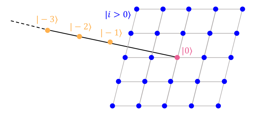
Figure 1: Illustration of the graph built by the algorithm in Table 1. A clean wire of length $L$ (orange nodes with negative indices) is coupled to the center of a lattice (pink node, denoted by $\Ket{0}$) of a $d$-dimensional lattice (Blue nodes with positive indices). Random potentials are then added to the lattice sites with positive indices. For clarity of the sketch, here $d=2$. However, note that the phase transition only occurs at $d>2$.

Initialization($E,\delta$):
0 $\leftarrow$ starting_site $c\leftarrow\text{small constant}\lesssim 1$ $C\leftarrow$large constant $\gg 1$
$\varepsilon\leftarrow$small constant $\ll 1$	Choose ancillary coefficients.
$k\leftarrow\cos^{-1}\frac{E}{2}$ $L\leftarrow\left\lceil\left(\delta^{\nu d}\varepsilon\right)^{-1}\right\rceil$ $H_{\text{wire}}\leftarrow\sum_{j=-L}^{0}\left(\Ket{j}\Bra{j+1}+\text{h.c}\right)$ $n\leftarrow\sum_{j=-L}^{0}\sin^{2}(kj)$ $\Ket{\psi_{0}}\leftarrow\frac{1}{\sqrt{n}}\sum_{j=-L}^{0}\sin(kj)\Ket{j}$ $H_{\text{clean}}\leftarrow\sum_{\langle i,j\rangle i,j>0}\Ket{i}\Bra{j}+\text{h.c.}$ $H\leftarrow H_{\text{wire}}+H_{\text{clean}}$	A disorder-free wire is added to the Hamiltonian, attached on one end to the 0 site. A single-particle normalized initial state is chosen as $\Ket{\psi_{0}}$, with an energy expectation value close to $E$ and level spacing small with relation to that of the system in the diffusive case (see discussion on the wire length in the main text). An illustration of the graph is given in Fig. 1.
$\xi_{E}\rightarrow\text{localization\_length}\left((E,c,\delta\right)$ $T\leftarrow\min\left\{t|\mathbb{E}_{\mathcal{P}_{W_{c}\left(1\boldsymbol{\boldsymbol{-}}\left|\delta\right|\right)}}\sum_{j\text{ }\text{s.t.}\text{ }\left|r_{j}-r_{0}\right|\geq\lceil C\xi_{E}\rceil}\left[\left|\Braket{\psi_{0}}{e^{i\left(H+\sum_{i}\epsilon_{i}\Ket{i}\Bra{i}\right)t}}{j}\right|^{2}\right]\geq c\right\}$	Choose a time $T$ long enough for a diffusive particle to reach a distance of $C\xi_{E}$ from the 0 site with probability $c$. From Eqs. (4),(5) it can be deduced that
$T=O\left(\left(C\xi_{E}\right)^{2}/D(E)\right)=O\left(\delta^{-\nu d}\right)$
$P_{\text{exp},d}=\mathbb{E}_{\mathcal{P}_{W_{c}\left(1\boldsymbol{\boldsymbol{-}}\delta\right)}}\left[\sum_{j\text{ }\text{s.t.}\text{ }\left|r_{j}-r_{0}\right|\geq\lceil C\xi_{E}\rceil}\left|\Braket{\psi_{{}_{0}}}{e^{i\left(H+\sum_{i}\epsilon_{i}\Ket{i}\Bra{i}\right)T}}{j}\right|^{2}\right]$
$P_{\text{exp},l}=\mathbb{E}_{\mathcal{P}_{W_{c}\left(1+\delta\right)}}\left[\sum_{j\text{ }\text{s.t.}\text{ }\left|r_{j}-r_{0}\right|\geq\lceil C\xi_{E}\rceil}\left|\Braket{\psi_{{}_{0}}}{e^{i\left(H+\sum_{i}\epsilon_{i}\Ket{i}\Bra{i}\right)T}}{j}\right|^{2}\right]$	Based on Eqs. (2) and (4), find the expected probability that a particle reached a distance $C\xi_{E}$ in the localized and delocalized phases, respectively.
determine_delta_sign($\mathcal{P}$):
$\text{{for }}i\text{ {in }}\left\{i|i>0\left|r_{i}-r_{0}\right|\leq C\sqrt{D(E)T}\right\}\text{ {do}}$
$\quad\epsilon_{i},\leftarrow\text{{Sample}}\left(\mathcal{P}\right)$
$\quad H.\text{append}\left(\epsilon_{i}\Ket{i}\Bra{i}\right)$
	Construct a Hamiltonian of a subsystem of volume $\left(C\sqrt{D(E)T}\right)^{d}=O\left(\delta^{-\nu d}\right)$. Based on Eq. (4) we see that the amplitude on sites $i$ for which $\left|r_{i}-r_{0}\right|\geq\sqrt{D(E)T}$ decays exponentially, and therefore considering a graph of this size will result in a good separation of the phases.
$\Ket{\psi(T)}=\exp\left(-iHT\right)\Ket{0}$
$P_{C\xi_{E}}=\sum_{j\quad\text{s.t.}\quad\left|r_{j}-r_{0}\right|\geq\lceil C\xi_{E}\rceil}\left|\Braket{\psi(T)}{j}\right|^{2}$	Calculate the state $e^{-iHT}\Ket{\psi_{0}}$, and from it deduce the probability for a particle to be at a distance larger than $\lceil C\xi\rceil$.
if $\left|P_{C\xi_{E}}-P_{\text{exp},d}\right|>\left|P_{C\xi_{E}}-P_{\text{exp},l}\right|$ do    return $\delta<0$.
else do
return $\delta>0$.	If the particle has reached a distance of $\lceil C\xi\rceil$ or more with high probability, we assume that the simulated system in the diffusive phase and $\delta<0$. Otherwise, we assume $\delta>0$.

Table 1: The suggested algorithm that utilizes the AL transition in order to differentiate the probability distributions. The algorithm is on the left column, and on the right we add explanations and reasoning.

Let us analyze the dependence of $N$ in the algorithm in Table 1 on $\delta$. A particle’s evolution is simulated only up to a finite time $T$. $T$ was chosen such that the number of site is proportional to $\xi_{E}^{d}$, so only $\Theta\left(\xi_{E}^{d}\right)$ sites, that is, $N=\Theta\left(\xi_{E}^{d}\right)$ samples, need to be considered. Comparing with Eq. (7), we obtain the result

$$\xi_{E}^{d} =\Theta\left(\delta^{-\nu d}\right)=\Omega\left(\delta^{-2}\right)$$ (9)

$$\Rightarrow \nu\geq\frac{2}{d}.$$

We see, therefore, that we have gained the results solely based on an information-theoretical argument.

The algorithm may fail if the local potentials drawn from $\mathcal{P}_{W(1\pm\delta)}$ results locally in the opposite phase as expected, that is, delocalization if $\delta>0$ or vice versa. However, repeating the process would decrease the probability for it up to an arbitrarily small one, exponentially fast in the number of repetitions.

II.3 Additional results

We first note that one may use other observables to differentiate between the localized and delocalized phase and derive the same bound $\nu\geq 2/d$. For example, one may diagonalize the Anderson Hamiltonian classically and examine whether the eigenfucntions are localized, using, e.g., the the inverse participation ratio. Using such an approach one may address the non-Anderson transition in Weyl and related systems [61], and derive the bound $1/z\geq 2/d$, with $z$ the relevant dynamic exponent, which was empirically found to hold [62].

One may also extend our argument to the classical system originally considered by Harris [16], namely a ferromagnetic Ising model in $d$ space dimensions, with a small random addition $\Delta J$ to the exchange coupling $J$. If one is at a dimensionless temperature distance $\delta_{T}\equiv(T-T_{c})/T_{c}$ from the critical temperature $T_{c}$, the correlation length is $\xi\sim|\delta|^{-\nu}$ in the clean case. Spins in regions of size $\sim\xi^{d}\sim|\delta|^{-\nu d}$ are thus correlated. The average disorder in such a region will be of order $\xi^{d/2}$, leading to a correspondingly large shift in $\delta_{T}$. This shift is small with respect to the staring value of $\delta_{T}$, making the criticallity robust to small disorder, only if $\nu\geq 2/d$.

One may rederive this result using our approach: Making the realistic assumption that small disorder shifts $T_{c}$ with some smooth dependence on the disorder distribution width, one may define a hypothetic decision problem differentiating two probability distributions of widths $W(1\pm\delta)$. A classical computer may use, e.g., classical Monte Carlo simulations to simulate such a system and determine whether it is paramangetic of ferromagnetic at an appropriately chosen temperature, and thus deduce whether the distribution width. The required system size (number of disorder samples) is $\sim\xi^{d}$, as above, leading again to the bound $\nu\geq 2/d$.

III Many-body localization

After presenting our method in the previous section, we now turn to apply it to the MBL phase transition and obtain bounds on the critical exponents that characterize it. In Sec. III.1 we briefly present the model as studied in configuration space and in Fock space. In Sec. III.2 we discuss bounds obtained by the method, and show that they are violated by numerical results. We discuss this discrepancy, and relate it to the ongoing discussion regarding the nature of MBL in infinite-sized systems. We derive additional new results for disordered interacting systems which are not covered by the MBL paradigm in Sec. III.3.

III.1 The Many Body Localization phase transition

Adding interaction to single-particle models in which all single-particle states are Anderson-localized may reintroduce ergodicity to the system: A localized particle may be ’pulled’ from its position by an interacting particle. In the energy spectrum, this is manifested by a broadening of energy bands. However, for a given interaction strength, it is widely agreed that one may still define a critical disorder above which the system is in a localized phase, at least in 1D[25, 26, 27]. We introduce here an example for a model which displays MBL, as studied, among other works, in Refs. [63, 64]:

$$H=\sum_{i=1}^{N-1}\left[\Delta\sigma_{i}^{z}\sigma_{i+1}^{z}+\frac{\sigma_{i}^{+}\sigma_{i+1}^{-}+\sigma_{i}^{-}\sigma_{i+1}^{+}}{2}\right]-\sum_{i=1}^{N}h_{i}\sigma_{i}^{z},$$ (10)

where $h_{i}$ are i.i.d random variables distributed by the probability distribution $\mathcal{P}_{W}$ as in the Anderson case. The model can be immediately transformed to describe spinless fermions by applying a Jordan-Wigner transformation[65]. The localized phase is characterized by site clusters which are resonantly linked, their size proportional to an MBL localization length $\xi_{\text{MBL}}$ . MBL is a more realistic model for studying disordered physical systems, and is also studied in the context of quantum technology as a candidate for quantum memory.

When a local perturbation occurs in the system, it is expected to spread across those clusters so that the effect of a local perturbation on site $i$ on a local observable on site $j$ decays exponentially as $\exp\left(-\left|i-j\right|/\xi_{\text{MBL}}\right)$. We define the critical exponent $\nu_{\text{MBL}}$ as

$$\xi_{\text{MBL}}\sim\delta^{-\nu_{\text{MBL}}},$$ (11)

where $\delta=W-W_{c}$ and $W_{c}$ is the critical disorder of the interactive model.

A more recent and enlightening angle for the study of MBL is studying the behavior of the system in Fock space: the system can be thought of as a single particle scattered across the graph defined by the disordered Hamiltonian in FS. The study of MBL as FS localization allows for the use of single-particle techniques, and sheds light on MBL behavior [67, 68, 69, 70, 71]. In FS, the Hamiltonian can be written as Eq. (1) with correlated local potentials: the number of sites in FS is $2^{N}$, but their random local potentials depend only on the $N$ parameters $\left\{h_{i}\right\}_{i=1}^{N}$.

In analogy to previous treatment of AL [72], and following in particular Ref. [73], Ref. [63] introduces a FS localization measure for an eigenstate $\Ket{\psi_{E}}$ with energy $E$:

$$S_{q}\left(\Ket{\psi_{E}}\right)=\frac{1}{1-q}\ln\left(\sum_{\alpha=1}^{\mathcal{N}}\left|\Braket{\psi_{E}}{\alpha}\right|^{2q}\right),$$ (12)

where $\mathcal{N}$ is the Hilbert space size and equals $2^{N}$ in our example. $S_{2}$ is also known as the inverse participation ratio (IPR). Using finite-size Scaling arguments, Ref. [63] describes the behavior of $S_{q}$ near the critical point:

$$\overline{S_{q}}\left(\Ket{\psi_{E}}\right)-\overline{S_{q,c}}\left(\Ket{\psi_{E}}\right)=\begin{cases}\mathcal{G}_{\text{vol}}\left(\frac{\mathcal{N}}{\Lambda_{q}{(d)}}\right)&\text{Delocalized}\\ \mathcal{G}_{\text{lin}}\left(\frac{\ln\mathcal{N}}{\xi_{q}{(d)}}\right)&\text{MBL}\end{cases},$$

where $\overline{\cdot}$ is the disorder average and $\Lambda_{q},\xi_{q}$ are emergent scales, dependending on the real-space lattice dimension $d$. In the ergodic (delocalized) phase, the state is close to being spread evenly across the entire FS, and therefore $S_{q}$ scales with FS volume. In the many-body localized phase, the particle in FS experiences long-range correlations, due to the fact the the disorder is correlated in that space. It will therefore not be in a localized but in a critical phase, with $\overline{S_{q}}\left(\Ket{\psi_{E}}\right)-\overline{S_{q,c}}\left(\Ket{\psi_{E}}\right)=-D_{q}\left(\ln\mathcal{N}/\xi_{q}\right)$ where $D_{q}$ can be called a fractal dimension. The above is organized in Refs. [63, 70] to obtain

$$\overline{S_{q}}\left(\Ket{\psi_{E}}\right)=\begin{cases}\ln\mathcal{N}+b_{q,\text{erg}}&\text{Ergodic (delocalized)}\\ D_{q}\ln\mathcal{N}+b_{q,\text{MBL}}&\text{MBL}\end{cases},$$ (13)

where $b_{q,\text{erg}}$ goes to zero near the critical point, $D_{q}$ goes to a critical fractal dimension, $D_{q,c}$, and $b_{q,\text{MBL}}$ remains constant:

$$D_{2}-D_{2,c} \sim\delta^{-{d}\beta},$$

$$b_{2,\text{erg}} \sim\delta^{-{d}\alpha},$$

$$b_{2,\text{MBL}} \sim\text{const.},$$ (14)

introducing two critical exponents, $\alpha,\beta$.

III.2 Many-body localization transition: Inconsistency with limited-sized system numerical results

Using scaling arguments equivalent to those in Refs. [23, 24], Refs. [74, 75] argued that $\nu_{\text{MBL}}$ is also bounded by the Harris criterion, Eq. (6), and indeed, for $d=1$ renormalization group methods yield $\nu_{\text{MBL}}\approx 3.3$[76, 77]. Along with the works above, we see that the protocol suggested in Table 1 may apply to MBL instantly, requiring only to change the single particle position to a single local perturbation position. We thus expect that for smooth distributions, the critical distribution would be bounded by Eq. (9). This is consistent with Refs. [74, 76, 77], but stands in contradiction to numerical results obtained for limited-sized systems: Refs. [28, 29] simulate a disordered one-dimensional system, and following Eq. (6), one would expect to get $\nu\geq 2$. However, in both cases the obtained critical exponent is $\nu\approx 0.9$, which raises the question whether the simulation results describe asymptotic behavior.

This discrepancy between theory and numerical results may be explained by Refs. [32, 30, 31, 34, 33, 35, 37, 36, 49, 48, 52, 51, 44, 45, 46, 47, 50]: in very large systems, it is expected that some subsystem of size $\sim\xi_{\text{MBL}}^{d}$ will randomly have lower disorder than $W_{c}$ even if the disorder distribution corresponds to the localized phase. This subsystem will thus thermalize, which in turn would lead to the thermalization of its surroundings. The new thermalized region would then thermalize its surroundings as well, resulting in an avalanche of thermalization which destroys the localization. The phase transition then changes its character, becoming a Kosterlitz-Thouless transition, where the localization length depends exponentially on $\delta$ (infinite critical exponent). Today’s numerically available systems sizes cannot display the phenomenon described here. Our result supports the above with a robust argument against the observed second order phase transition phenomenology, an argument which does not relying on any heuristic reasoning.

Initialization($E,\left|\delta\right|,\mu$):
0 $\leftarrow$ starting_site $N\leftarrow\lceil\delta^{-\mu}\rceil$ $\mathcal{N}\leftarrow d_{\text{single}}^{N}$
$H\leftarrow H_{\text{clean}}(N)$	Choose ancillary coefficients. Choose a system length $N=\delta^{-\mu},$where $\mu$ is discussed in the main text. Start with the $N$-particle disorder-free Hamiltonian, as defined, for example, in Eq. (10). $d_{\text{single}}$ denotes the Hilbert space size of a single site.
determine_delta_sign():
for $i$ in $1..N$ do $\quad h_{i}\leftarrow\text{{Sample}}\left(\mathcal{P}\right)$ $\quad H.\text{append}\left(h_{i}\sigma_{i}^{z}\right)$	Add the disorder to the Hamiltonian by performing $N$ samples from the distribution.
$\Ket{\psi_{E}}\leftarrow\text{{eigenvector}$\left(H,E\right)$}$ $S_{2}\leftarrow-\ln\left(\sum_{\alpha=1}^{\mathcal{N}}\left|\Braket{\psi_{E}}{\alpha}\right|^{4}\right)$	Diagonalize $H$ to obtain the eigenvector with the maximal eigenvalue $\leq E$ and calculate its IPR.
If $\left|\frac{S_{2}}{\ln\mathcal{N}}-\left(1+\frac{b_{2,\text{erg}}(\delta)}{\ln\mathcal{N}}\right)\right|<\left|\frac{S_{2}}{\ln\mathcal{N}}-\left(D_{2}(\delta)+\frac{b_{2,\text{MBL}}(\delta)}{\ln\mathcal{N}}\right)\right|$ do    return $\delta<0$. else do    return $\delta>0$.	Determine the phase of the simulated system based on the calculated IPR.

Table 2: The suggested algorithm that utilizes the FS localization transition in order to differentiate the probability distributions. The algorithm is on the left column, and on the right we add explanations and reasoning.

As for the behavior in FS, the critical exponents have still been expected to behave as Eq. (14). In Refs. [73, 78], a localization length in FS is defined and assumed to obey the same critical exponents as the real space localization length, in order to bound the FS behavior using the Harris criterion. Here, we obtain an equivalent bound without relying on any assumption: We generalize our argument to apply to the FS localization transition in Table 2. Following Eq. (13), we suggest an algorithm that performs $N=\delta^{-\mu}$ samples from the distribution $\mathcal{P}_{W\left(1\pm\left|\delta\right|\right)}\left(h_{i}\right)$ and uses them to define an $N$-site Hamiltonian as in Eq. (10). The Hamiltonian is then diagonalized and the IPR computed. The probability distribution is then determined based on the proximity of the IPR extracted from the simulated system and the expected IPRs for both phases. Note that below we bound $\mu$ as a function of $\alpha,\beta$ and not the other way around as above, and following Eq. (7), we require that the result would be $\mu\geq 2$.

We analyze the requirements for the success of the protocol presented in Table 2. We first define $\Delta S_{2}$ to be the deviation of $S_{2}$ from $\overline{S_{2}}$. The protocol is successful if

$$\Delta S_{2}/\ln\mathcal{N} \ll\left|\overline{S_{2,\text{erg}}}-\overline{S_{2,\text{MBL}}}\right|/\ln\mathcal{N}$$

$$=\left|1-D_{2}(\delta)+\frac{b_{2,\text{erg}}(\delta)}{\ln\mathcal{N}}-\frac{b_{2,\text{MBL}}(\delta)}{\ln\mathcal{N}}\right|.$$ (15)

From Eq. (14), we write the dependence of each term in Eq. (15) on $\delta$. Substituting these dependancies into the requirement in Eq. (15), it becomes

$$\Delta S_{2}/\ln\mathcal{N} \ll\left|O(1)+O\left(\delta^{-d\alpha+\mu}\right)+O\left(\delta^{\mu}\right)\right|$$

$$=\begin{cases}O\left(\delta^{-d\alpha+\mu}\right)&\alpha>\mu{/d}\\ O(1)&\alpha<\mu{/d}\end{cases}.$$ (16)

However, The FS localization transition has been studied in Refs. [63, 64], for a one-dimensional system with a uniformly distributed disorder. The obtained critical exponents were $\alpha\approx 0.5,\beta\approx 0.76$, and the fluctuations $\Delta S_{2}/\ln\mathcal{N}\sim N^{-1/2}=\delta^{\mu/2}$. This implies that $\alpha\leq\mu\leq 1$ may be sufficient to obey Eq. (16) and differentiate the distributions, which contradicts our argument: it implies that simulating a many-body system with disorder and determining its phase is a better strategy for differentiating probability distributions than an explicit error evaluation. We stress again that we only compare sample complexity here (which measures the amount of information obtained regarding $\mathcal{P}_{W}$, and not computation time complexity). This leads us again to argue that the obtained critical exponents may not describe the near-critical behavior in infinite systems, implying that the limited-sized numerical result fail to fully simulate the asymptotic behavior of FS localization transition. This result is inline with recent numerical works which provide evidence that current numerically accessible system sizes might be too small to approach the thermodynamic limit [80, 81, 82, 83]

III.3 Additional results

Our approach allows for deriving additional interesting results. In the presence of long-range Coulomb interaction the phenomenology of localization is different than the standard MBL [84]. In particular, it is found that in the delocalized regime (but not in the localized one) a dephasing length appears, which might be shorter than the correlation length. Thus, systems of size smaller thant the correlation/localization length but larger than the dephasing length are predicted to display different behavior on the two sides of the transition, allowing one to use our methodology to derive a Harris-like bound on the dynamical critical exponent $z^{n}_{\phi}$ charaterizing the dephasing length, namely $1/z^{n}_{\phi}\geq d/2$. Intriguingly, this bound is not obeyed by the theoretical estimate provided for $z^{n}_{\phi}$ in Ref. [84] at $d=3$, which may result from the inadequacy of using the Fermi golden rule to estimate the dephasing length in this regime [85].

IV random circuits

IV.1 Measurement-induced phase transition in random circuits

Figure 2: Based on the illustration in Ref. [54]. The random circuit model is composed of layers of random unitaries (blue rectangles), interchanged by layers of projective measurements applied randomly with some probability $p$ (black circles). Performing a measurement may be treated as cutting the qubit line in the position of the black circle, demonstrating the relation of the phase transition to that of a percolation problem.

In this section we apply our bounding method to measurement-induced phase transition in quantum circuits. Apart from the distinction of phases by disorder, these models are unrelated to localization, thus demonstrating the generality of our method. Quantum circuits subject to random measurements[53, 54, 55, 56] provide a generic model for open systems interacting with an environment, motivated both by quantum technology and many-body physics. In recent years, different settings of such circuits have been heavily studied theoretically and numerically [86, 87, 88, 89, 90, 91, 92, 93, 94, 95, 96, 97] as well as experimentally[98, 99], presenting new insights regarding the behavior of open systems. The unitary gates in the circuit create entanglement between qubits, while the random measurements ruin it. This competition leads to an entanglement phase transition, with the measurement probability as an order parameter.

As a basic example model, consider the following setting: We start with a register of $L^{d}$ qubits, organized as a $d$-dimensional lattice of length $L$. $t$ layers of spatially local random 2-qubit unitary gates are then applied to the qubits, where in between each layer, each qubit is measured with probability $p$, see Fig. 2. For $p$ close to 1, the qubits decay frequently into a pure eigenstate of the computational basis, losing their ’quantumness’, and the resulting state has little entanglement, typically an area-law. For small values of $p$, the system is close to remaining pure, with a volume-law entanglement between a subsystem and its complement in the average case[53, 54]. A phase transition occurs at some critical value $p_{c}$.

The two phases are characterized by the entanglement between two parts of the system, denoted by $A$ and $\overline{A}$. A standard measure of entanglement is the von Neumann entropy, $\mathcal{S}(\rho_{A})=-\mathrm{Tr}\left(\rho_{A}\log\rho_{A}\right)$, where $\rho_{A}=\mathrm{Tr}_{\overline{A}}\left(\rho\right)$ is the reduced density matrix of $A$. Due to the numerical inaccessibility of the von Neumann entropy, Rényi entropies are also introduced,

$$\mathcal{S}_{n}(\rho_{A})=\log\left(\mathrm{Tr}\left(\rho_{A}^{n}\right)\right)/(1-n),$$ (17)

which obey $\lim_{n\rightarrow 1}\mathcal{S}_{n}(\rho_{A})=\mathcal{S}(\rho_{A})$. The Rényi entropies are entanglement monotones, and for $n>0$ they are smooth and able to reflect small changes in the entanglement accurately.

We observe the case where $t\sim L^{z}$ ($z$ being the dynamical critical exponent), such that the circuit may be thought of as a $d+1$ dimensional system (anisotropic for $z\neq 1$). We follow Ref. [54] and define the characteristic length scale $\xi_{\text{RC}}^{(n)}$ and time (circuit depth) scale $\tau_{\text{RC}}^{(n)}$ by

$$S_{n}\left(\rho_{A}(L,p)\right)-S_{n}\left(\rho_{A}(L,p_{c})\right)=f\left(\frac{L^{d}t}{\left[\xi_{\text{RC}}^{(n)}\right]^{d}\tau_{\text{RC}}^{(n)}}\right),$$ (18)

in the limit of large $L,t$, where $f$ is a scaling limiting behavior. We then assume a second order phase transition:

$$\xi_{\text{RC}}^{(n)} \sim\delta^{-\nu_{\text{RC}}},$$

$$\tau_{\text{RC}}^{(n)} \sim\delta^{-z\nu_{\text{RC}}},$$ (19)

where $z=1$ in the presence of space-time symmetry.

We focus on the 0th Rényi entropy as an entanglement measure. When $n=0$, the Rényi entropy counts the nonzero eigenvalues of the reduced density matrix (Schmidt rank). $\mathcal{S}_{0}$ is a useful entanglement measure (for example, it represents the required bond dimension for the representation of the system as a matrix product state[10]), but it is highly sensitive to small, insignificant eigenvalues of $\rho_{A}$, and completely insensitive to a significant change of nonzero eigenvalues. In spite of its disadvantages, $\mathcal{S}_{0}$ is more amenable to theoretical analysis in the current case. This stems from the fact that from the point of view of $\mathcal{S}_{0}$, the problem can be described as a graph percolation problem, each measurement becoming a cut in the graph [100, 54]. This allows to leverage on the large body of knowledge on percolation problems [101]. We note in particular that a percolation phase transition must obey the Harris criterion in Eq. (6), with a denominator $d+1$ counting the spatial dimension $d$ of the system but also the time (circuit depth) dimension.

The behaviors of Rényi entropies for other values of $n$ near the phase transition were studied numerically for $1+1$ dimensions, and they seem to also obey the Harris criterion, although so far its validity had not been argued by any theoretical analysis we are aware of. It is interesting to note that the critical value $p_{c}$ extracted for $n\neq 0$ is different from the one extracted for $n=0$ (which matched the percolation critical value, $p_{c}=1/2$), suggesting that percolation is indeed not a good model for describing the behavior of general Rényi entropies, or that the numerically-observed behavior of $S_{n}$ for $n>1$ does not scale to large system sizes.

IV.2 Bounding the critical exponents

We may now apply our method to the critical exponents defined in Eqs. (19). Following the layout in Sec. II.2, the (hypothetical) decision problem may be differentiating two probability distributions over $\{0,1\},$where $p(1)=p_{c}(1\pm\left|\delta\right|)$. The required sample number $N_{\text{opt}}$ is then bounded by $N_{\text{opt}}=\Theta\left(\delta^{-2}\right)$ as before. An algorithm for differentiating the distributions may be simulating a random circuit of size $L^{d}$ and depth $t$ and computing $S_{n}$ for half the system. It is required that $L\gg\xi_{\text{RC}}^{(n)}$ and $t\gg\tau_{\text{RC}}^{(n)}$, i.e., the number of samples $N_{\text{PT}}=L^{d}t\gg\left[\xi_{\text{RC}}^{(n)}\right]^{d}\tau_{\text{RC}}^{(n)}\sim\delta^{-\nu_{\text{RC}}(d+z)}.$ We then bound the sample complexity in the phase-transition-based method by that of the optimal one, $N_{\text{PT}}\leq N_{\text{opt}}$, and obtain the bound

$$\nu_{\text{RC}}(d+z)\geq 2.$$ (20)

The obtained bound is obeyed numerically [54, 89, 102, 103]. As opposed to existing analytical results, it is not limited to $d=1$ or $n=0$ but is completely general.

We would like to point out a possibly peculiar point: the inequality above stems from the bound of the optimal utilization of samples. It therefore becomes an equality when the calculated measure, $\mathcal{S}$ or $\mathcal{S}_{n}$ in our case, utilizes the information extracted from the distribution in an optimal way. One can then assume that the tighter the bound, the less information is “wasted” in the process of computing $\mathcal{S}_{n}$. It could be expected, based on the discrete properties of $\mathcal{S}_{0}$, that the bound would be tighter for $n\neq 0$. However, when observing the numerical results of Ref. [54] for $d=1,n=0,1,2,\infty$, it seems that the opposite is true, which implies that the physical difference between the two distributions is more apparent in $\mathcal{S}_{0}$ than it is in $\mathcal{S}_{n\neq 0}$. It could be interesting to use this line of thought in order to study the amount of information represented in different entanglement measures.

Let us finally note that one may use other aspects of the measurement-induced transition, such as the purification transition [89], to derive similar bounds on the corresponding critical exponent $\nu$, independently of whether or not those transitions coincide.

V Conclusion and future outlook

In our work, we introduced a method of obtaining critical exponent bounds in phase transitions of disordered systems, combining information bounds with physical phenomena. Due to its generality and the fact that it does not require introducing physical or intuitive arguments, the bounds obtained by the method are robust. By construction it is suited for systems close to the critical point, that is, large systems sizes.

After benchmarking the method and rederiving the Harris criterion, we obtained bounds for MBL and FS localization transitions. Along with additional theoretical works before, we show that the MBL phase transition should obey the Harris criterion. We obtain new bounds on the critical exponents of the FS localization transition. The bounds in both cases above are contradicted by numerical results, implying that the behavior in limited-sized systems does not represent the behavior in infinite-sized systems. These results are relevant to the ongoing discussion regarding the asymptotic behavior of MBL[31, 32, 33, 35, 37, 38, 39, 40, 41, 42, 43, 44, 45, 46, 47, 48, 49, 50, 51, 52, 34, 36]. We add an argument that does not rely on any intuitive assumption and utilizes a different set of tools than former arguments in the discussion, proposing a contribution from a new angle. It may also apply to other types of FS transitions [104].

Additionally, we obtained a bound on critical exponents in measurement-induced phase transitions in random circuits, tying together the behavior of all entanglement measures in these transitions and expanding the spatial dimension of studied circuits. Our results are obeyed by existing numerical results, and may be expanded to extensions of the model, such as adding a ’reset’ probability [97], applying projective measurements which do not fully collapse the measured qubit’s state [93], or adjusting the unitary gates based on the measurements’ results [96]. It would be interesting to apply the method to the adjusted phase transitions in such variations.

The same line of thought may be applied to additional phase transitions, such as other forms of correlated disorder or interdependent networks[105, 106, 107, 108, 109, 110, 111]. It can be readily applied to other examples suggested in Ref. [23] or similar models, in which the randomness is presented on the hopping terms rather than local potentials. We believe that this is a road worth taking from an additional aspect: if a physical result similar to the above cannot be obtained for some model, this may imply a task that cannot be done by a classical computer but can be done with a quantum computer – a marker for quantum advantage.