Tuning the perplexity for and computing sampling-based t-SNE embeddings

Abstract

Widely used pipelines for the analysis of high-dimensional data utilize two-dimensional visualizations. These are created, e.g., via t-distributed stochastic neighbor embedding (t-SNE). When it comes to large data sets, applying these visualization techniques creates suboptimal embeddings, as the hyperparameters are not suitable for large data. Cranking up these parameters usually does not work as the computations become too expensive for practical workflows. In this paper, we argue that a sampling-based embedding approach can circumvent these problems. We show that hyperparameters must be chosen carefully, depending on the sampling rate and the intended final embedding. Further, we show how this approach speeds up the computation and increases the quality of the embeddings.

1 Introduction

In the ever-evolving landscape of data science and analytics, the exponential growth of available data has led to an era of unprecedented complexity, particularly in high-dimensional data sets. High-dimensional data, characterized by its abundance of variables, pose a unique challenge: the inherent limitations of the human mind in comprehending and interpreting data beyond three dimensions. As a result, effective visualization techniques become not only valuable but essential tools for gaining meaningful insights from such intricate data sets.

Specifically in the field of life sciences, the emergence of single-cell technologies has revolutionized the study of biological systems, allowing researchers to scrutinize cellular heterogeneity and understand the finer nuances of intricate cellular processes. Single-cell RNA sequencing (scRNA-seq), for instance, can produce a wealth of information on gene expression at the cellular level, providing insights into cell types, states, and trajectories. However, the sheer volume of data generated in scRNA-seq experiments often translates to high-dimensional spaces where traditional analysis methods fall short. Here, data visualization steps in as an indispensable aid, offering a bridge between the complexity of the data and human perceptibility. Visualization techniques empower researchers to identify clusters of cells, track dynamic changes, and uncover markers that drive cellular diversity, all of which are pivotal in deciphering the intricate mechanisms governing biological systems.

A prominent technique that has made a resounding impact on the visualization of high-dimensional data is t-distributed Stochastic Neighbor Embedding (t-SNE). As a non-linear dimensionality reduction method, it operates by modeling pairwise similarities between data points in high-dimensional space and iteratively adjusting the representation of data in a lower-dimensional space, often two-dimensional, to preserve these similarities. It excels at revealing local structures and is particularly effective in visualizing clusters and relationships within complex data sets.

An important hyper-parameter in the use of t-SNE is the perplexity. Roughly speaking, it tunes how many high-dimensional neighbors are considered for a point when evaluating its low-dimensional embedding. Previous work has found that in order to obtain high-quality embeddings, the perplexity should be chosen with a linear relation to the number of data points to be embedded [6, 8]. However, as the number of neighbors to be considered grows, the run-time of the algorithm also grows, which leads to impractical running times for large data sets. Therefore, current implementations tend to choose fixed perplexities that ensure reasonable run times, but are not necessarily tailored to the data set. Particularly, choosing a too low perplexity can completely fail the embedding computation [20]. In order to mitigate this problem, in the present article, we:

• …provide additional evidence for a linear relation between the size of a data set and the perplexity for its embedding.

• …use a sampling approach to compute embeddings with perplexity values larger than the state-of-the-art.

• …provide a method to quickly estimate a fitting perplexity value for large data sets.

• …discuss the speed-up obtained by the sampling approach, which comes without compromising embedding quality or quantitative measures.

• …show how sampling can improve neighborhood preservation.

2 Background and Related Work

A widely used technique for nonlinear dimensionality reduction is t-SNE, which creates a low-dimensional embedding of the data while aiming at preserving local neighborhoods of the high-dimensional data points [12]. This is achieved by interpreting the high-dimensional input ${\{\mathbf{x}_{1},\ldots,\mathbf{x}_{n}\}\subseteq\mathbb{R}^{d}}$ as (conditional) probabilities by

$$p_{j|i}=\frac{\exp\left(-\left\|\mathbf{x}_{i}-\mathbf{x}_{j}\right\|^{2}/2\sigma_{i}\right)}{\sum_{k\neq i}\exp\left(-\left\|\mathbf{x}_{i}-\mathbf{x}_{k}\right\|^{2}/2\sigma_{i}^{2}\right)},\quad p_{ij}=\frac{p_{j|i}+p_{i|j}}{2},$$ (1)

where $p_{i|i}=0$ and $\sigma_{i}$ is the variance of the Gaussian centered on point $\mathbf{x}_{i}$. In practice, the bandwidth $\sigma_{i}$ is chosen such that the perplexity of the probability distribution $P_{i}$ equals a user-prescribed perplexity value $\operatorname{Perp}$. On the low-dimensional embedding ${Q=\{\mathbf{y}_{1},\ldots,\mathbf{y}_{n}\}\subseteq\mathbb{R}^{d^{\prime}}}$, a corresponding probability distribution is given by

$$q_{ij}=\frac{\left(1+\left\|\mathbf{y}_{i}-\mathbf{y}_{j}\right\|^{2}\right)^{-1}}{\sum_{k\neq\ell}\left(1+\left\|\mathbf{y}_{k}-\mathbf{y}_{\ell}\right\|^{2}\right)^{-1}}.$$ (2)

In order to compute the positions $\mathbf{y}_{i}$ of the low-dimensional embedding, t-SNE starts with an initial embedding obtained by principal component analysis (PCA) [9] and then alters the embedding by gradient-descent optimization of the Kullback-Leibler divergence between the high- and the low-dimensional probability distribution, which is given by

$$C=\operatorname{KL}(P||Q)=\sum_{i}\sum_{j}p_{ij}\log\frac{p_{ij}}{q_{ij}},$$ (3)

with the gradient

$$\frac{\partial C}{\partial\mathbf{y}_{i}}=4\sum_{j\neq i}(p_{ij}-q_{ij})\left(1+\left\|\mathbf{y}_{i}-\mathbf{y}_{j}\right\|^{2}\right)^{-1}(\mathbf{y}_{i}-\mathbf{y}_{j}).$$ (4)

The naive implementation of t-SNE has a run time of $\mathcal{O}(n^{2})$. Therefore, several acceleration structures have been proposed. A wide-spread acceleration is given by the Barnes-Hut (BH) tree structure [19]. The main idea is that the gradient can be split into terms representing the attractive and terms representing the repulsive forces. The former are then naturally fast to evaluate, assuming that the probability matrix $P$ is sparse. To approximate the latter, a quad tree is built on the embedding of the data points. Then, when evaluating the gradient, those terms involving a low-dimensional computation of $q_{ij}$ are approximated by aggregating point-wise terms by centers of tree nodes. Thereby, the run-time becomes log-linear.

An alternative is given by Fast-Fourier Transform [10]. Here, the domain is discretized and the forces are first computed on the discrete nodes in the domain. Then, for each embedding point, the forces are approximated from the surrounding nodes. Thereby, the run-time becomes independent from the number of points, but still depends on the number of nodes to take into account.

Other acceleration structures are available that utilize the GPU functionality [16, 17]. However, we focus on acceleration structures that can be utilized without specific hardware requirements. In addition to t-SNE, UMAP provides another popular method of creating embeddings [13, 1]. However, due to its use of stochastic gradient descent, it is not possible to find a strong correlation between the neighborhood size hyper parameter of UMAP and the embedding, as is possible and performed in this paper for t-SNE. Furthermore, recent work suggests that UMAP-type embeddings are merely a part of a spectrum of embeddings, attainable via t-SNE [3, 5]. Thus, the following discussion will be restricted to t-SNE. In the context of t-SNE, a hierarchical method has been previously introduced [18]. However, the hierarchies are tailored to enhance visual tasks, not the performance of the embedding itself.

3 Methods

As stated above, an important element of t-SNE is the nearest neighbor graph, which the embedding algorithm needs to construct in order to be able to evaluate the objective function. Along the edges of this graph, attracting forces act and hold the points in the embedding space together like a network of springs. This structure inspires us to use graph-based multigrid methods for the t-SNE problem. We will borrow concepts and terminology from graph-based algebraic multigrid approaches to build a two-level t-SNE hierarchy and operators between the levels. In doing so, we are inspired by the success of hierarchical solvers for problems in several fields, such as fluid dynamics [15], computational physics [4], or mechanical engineering [14]. In particular, algebraic multigrid methods, such as the Lean Algebraic Multigrid [11], proved to be efficient for large graph-Laplace problems. However, unlike these linear problems, the t-SNE problem is non-linear, which needs to be taken into account by the hierarchical solver.

In general, the approaches listed above do not immediately compute a solution for the PDE problem on the domain, but rather start with a coarser domain, quickly derive a solution there, and then propagate this solution onto the desired fine domain. Following this general concept, our pipeline consists of the following steps:

1. Initialization: Start with a fine data set and an intended perplexity $\operatorname{Perp}$.

2. Restriction: Downsample the data set to a size that is as small as possible while still representing all structures; call this the coarse data.

3. Optimization: Compute an embedding of the coarse data using an adjusted perplexity $\operatorname{Perp}^{\prime}$.

4. Prolongation: Prolongate the coarse embedding to the fine data set by placing all remaining points around their nearest, high-dimensional neighbors.

5. Smoothing: Run some further iterations of the gradient descent to smooth the fine embedding obtained.

Note that a related approach was proposed in [8], yet not executed. Additionally, we will propose a concrete methodology on how to choose a suitable perplexity $\operatorname{Perp}$ for the fine level as well as how to alter this perplexity on the coarse level in order to obtain high-quality embeddings. This is different to the scheme of combined or fixed perplexities on the different levels, as previously proposed [8]. We will now discuss the different steps of our method in detail.

3.1 Initialization and choosing perplexity $\operatorname{Perp}$

The method starts with a user-provided data set as well as a user-chosen perplexity $\operatorname{Perp}$ for these data. When choosing the perplexity $\operatorname{Perp}$, the user can follow a heuristic presented in previous work and choose ${\operatorname{Perp}=n/100}$ [8] or ${\operatorname{Perp}=10n/512}$ [6], where $n$ is the number of data points to be embedded. Alternatively, as perplexity also steers some embedding properties that are more a matter of taste, for example, how spread out a data cluster should be, we propose the following scheme to choose $\operatorname{Perp}$.

Choose a low sampling rate ${\rho\in(0,1]}$ such that a sample of size ${\rho n}$ can be embedded quickly. Then perform the embedding as described in the following section. Because this embedding can be obtained quickly, it is possible to perform this optimization several times, with varying perplexity values $\operatorname{Perp}^{\prime}$. As we will see below, embedding the $\rho$-sample of the data with perplexity $\operatorname{Perp}^{\prime}$ gives a visual impression of embedding the fine data with ${\operatorname{Perp}=\operatorname{Perp}^{\prime}/\rho}$. Thus, the user can choose a suitable perplexity $\operatorname{Perp}$ without having to go through the costly process of embedding the fine data set several times for different perplexities.

3.2 Restriction

Having chosen an initial perplexity $\operatorname{Perp}$, the user has to choose a sampling rate ${\rho\in(0,1]}$, which might be given by the exploratory search for a suitable $\operatorname{Perp}^{\prime}$. In any case, $\rho$ should be chosen small enough such that the calculation of a coarse embedding on ${\rho n}$ points can be performed quickly. Given $\rho$, from the fine data, we draw a uniform random sampling of size $\rho n$. The sampling is chosen uniformly random because it can be proven: There exists a (large enough) subset $S$ of a point set $P$, such that $S$ is an $\varepsilon$-net of $P$ with high probability, given a random sampling [7]. That is, every point $p\in P$ has an element $s\in S$ in its $\varepsilon$-neighborhood, providing good coverage over the original data. Note that this statement is independent of $P$, in particular of the distribution of the points in $P$ [7].

As we use a uniform random sampling approach, this suggests the following scheme to alter the neighborhood sizes: If on the fine level, we aim to work with a neighborhood of $k$ points, this fixes a certain distance $d_{i}$ around each point ${i\in[n]}$. After random sampling the points by a sampling factor ${\rho\in(0,1]}$, we expect to find ${\rho k}$ many sampling points within distance $d_{i}$ of point $i$, provided that $i$ was chosen in the sampling. Hence, if we aim for an embedding using neighborhood size $k$ on the fine level, we have to run it with ${\rho k}$ on the coarse level. We will make this more explicit in the following.

We will first consider the discrete case, i.e., a neighborhood size $k$ is given or derived as ${k=\min\{N,3\cdot\operatorname{Perp}\}}$ following [19]. For a given point ${x_{i}\in D}$, its $k$-nearest neighbors ${\{x^{\prime}_{1},\ldots,x^{\prime}_{k}\}}$ define a geometric neighborhood ball of radius ${d(x_{i},x^{\prime}_{k})}$, assuming that $x^{\prime}_{k}$ is the farthest neighbor among the $k$-nearest. When restricting to a uniformly chosen subset $S$ of $D$, picking each point with probability ${\rho\in(0,1]}$, the expected number of points to lie within the ${d(x_{i},x^{\prime}_{k})}$-ball around $x_{i}$ is exactly $\rho k$. Hence, in order to provide point $x_{i}$ with the same geometric information, that is, having all neighbors within the ${d(x_{i},x^{\prime}_{k})}$-ball with high probability, we have to choose a neighborhood size of $\rho k$ or a perplexity of $\rho\operatorname{Perp}$ respectively.

In the continuous case, a perplexity $\operatorname{Perp}$ is given and for each point $x_{i}$, a bandwidth value $\sigma_{i}$ is chosen according to

$$p_{j|i}=\frac{\exp\left(-d(x_{i},x_{j})^{2}/2\sigma_{i}^{2}\right)}{\sum_{k\neq i}\exp\left(-d(x_{i},x_{k})^{2}/2\sigma_{i}^{2}\right)},$$ (5)

such that

$$\operatorname{Perp}=\operatorname{Perp}(p_{i})=2^{-\sum_{j}p_{j|i}\log(p_{j|i})}.$$

When drawing a random sample from the input data, in order to not distort the embedding by the sampling process, we want to choose a coarse perplexity $\operatorname{Perp}^{\prime}$ such that the points’ individual bandwidths $\sigma_{i}$ remain the same under the sampling, i.e., such that the geometric neighborhood of each point has the same extend. That is, we draw a sample ${S\subseteq D}$ of points from $D$, where each point $x_{i}$ is chosen with some uniform probability ${\rho\in(0,1]}$. Then, we want to choose a perplexity $\operatorname{Perp}^{\prime}$ for the sample such that the $\sigma_{i}$ are as close as possible to the ones for the full data set with $\operatorname{Perp}(p_{i})$ with high probability. To determine the perplexity $\operatorname{Perp}^{\prime}$ suitable for a specific point $x_{i}$ of the sampling, consider the ${i\in[n]}$ fixed and take into account the following set of random variables:

$$X_{j}=\begin{cases}\exp\left(-d(x_{i},x_{j})^{2}/2\sigma_{i}^{2}\right)&\rho\\ 0&1-\rho\end{cases},$$

which are Bernoulli variables taking value ${c_{j}=\exp\left(-d(x_{i},x_{j})^{2}/2\sigma_{i}^{2}\right)}$ with uniform probability $\rho$ and value $0$ otherwise. Note that this uses the same established bandwidth $\sigma_{i}$ as before, i.e., each point $x_{i}$ will be influenced by the same geometric neighborhood. These give rise to a new set of random variables

$$P_{j|i}=\frac{X_{j}}{\sum_{k\neq i}X_{k}}.$$

Then, we can describe the sought-for perplexity $\operatorname{Perp}^{\prime}$ for the sample point $x_{i}$ as:

$$\begin{split}\operatorname{Perp}^{\prime}(p_{i})&=\mathbb{E}\left(2^{-\sum_{j}P_{j|i}\log(P_{j|i})}\right)\\ &=\mathbb{E}\left(2^{-\sum_{j}\frac{X_{j}}{\sum_{k\neq i}X_{k}}\log\left(\frac{X_{j}}{\sum_{k\neq i}X_{k}}\right)}\right).\end{split}$$ (6)

Sadly, this expression is not straight-forward to be analyzed analytically. Preliminary experiments show that our linear scaling is a suitable approach, as shown in our experimental evaluations, see Section 4.1. However, Equation (6) could possibly be evaluated via a Monte-Carlo approach, which we leave as future work.

3.3 Computation of a coarse embedding

Having restricted to a coarse set $S$ of data and having chosen a perplexity $\operatorname{Perp}^{\prime}$, we perform a standard t-SNE embedding. That is, we initialize the procedure with a PCA embedding of $S$ [9]. However, to capture as much structure as possible, we do not perform PCA on $S$ directly. Instead, we compute a PCA embedding of $P$ and restrict this embedding to $S$ for initializing t-SNE. Then, we first run a set of $250$ iterations of early exaggeration, followed by $750$ iterations of regular, non-exaggerated gradient descent. For the learning rate $\eta$, we follow the state of the art and set it to $\eta=n/12$ [2], which is then further optimized by the use of momentum and gain [12]. As acceleration technique, both Fast-Fourier Transformations [10] and the Barnes-Hut tree structure [19] can be used. The former scales linearly with the perplexity used, while the latter scales with the number of points. Both thus provide an embeddings of $S$ with perplexity $\operatorname{Perp}^{\prime}$ faster than an embedding of the entire data set with perplexity $\operatorname{Perp}$.

3.4 Prolongation

Once we computed an embedding for the coarse data set $S$, we prolongate the embedding to the fine data set as follows. For each point ${x_{i}\notin S}$, find the nearest neighbor to $x_{i}$ in $S$, i.e., $\operatorname*{arg\,min}_{s\in S}d(s,x_{i})$, based on the high-dimensional distances $d$. Then, we place each such point $x_{i}$ at the embedding location of $s$. While this causes high cost-function values as the repulsive forces try to drive the points away from each other, it ensures that local neighborhoods are preserved.

3.5 Smoothing

As a final pass on the data, we apply several iterations of gradient descent on the embedding obtained after prolongation. This is to smooth out any high-frequency errors introduced by prolongation. Our experiments show that the global shape of the embedding is fully determined by the shape of the coarse embedding, hence the smoothing step only reduces clutter after prolongation. Furthermore, since the structure has been settled in a way or another, it satisfies to run these steps with a rather low perplexity, e.g., $30$. It is not necessary to perform them with the desired perplexity $\operatorname{Perp}$ as the choice of $\operatorname{Perp}^{\prime}$ and the prolongation already ensure that the structures are in place that would correspond to embedding the data with perplexity $\operatorname{Perp}$ from scratch.

4 Results

4.1 Perplexity scales linearly with point set size

From what we reasoned above, given a data set and several different perplexities, each of these will create a different embedding of the data. However, given the linear relationship between perplexity and number of points $n$, the embedding is qualitatively stable under a uniform sampling of the data by a factor of ${\rho\in(0,1]}$ and a corresponding reduction of the perplexity. That is, when keeping the ratio between perplexity and number of data points constant over several different sample sizes, their respective embeddings remain qualitatively similar.

As a toy data set to see this effect, we turn to the MNIST data of ${n=70,000}$ images of handwritten digits. Various t-SNE embeddings of the data set are shown in Figure 1. To focus on the effect of the chosen perplexity, all embeddings are derived from a shared initialization, obtained via PCA [9], which is sampled according to the number of points.

Furthermore, samples, in each column are nested to ensure direct comparability. That is to say that, when drawing the sample of, e.g., the third row of the first column, it is not drawn from the entire data set, but it is drawn from the sample represented in the second row. While we draw uniform samples that should represent the data equally well, in order to be able to visually compare the outcomes, we opt for this nested sampling approach.

Each t-SNE run was executed with fast Fourier transform t-SNE, 250 iterations of early exaggeration (exaggeration factor 12, momentum 0.5) and 750 iterations of gradient descent (exaggeration factor 1, momentum 0.8). This is following the standard parameters as used in, e.g., SciKit Learn or OpenT-SNE. We present the obtained embeddings in Figure 1. In each column, from top to bottom, we increase the number of points from the data set to be embedded, while keeping the ratio of perplexity and number of points constant. In the rows, from left to right, we increase this ratio. While the embeddings are qualitatively quite different across each of the rows—e.g., in terms of placement, shape, or entanglement of the clusters—they are stable within each column, as the theoretical derivation predicts.

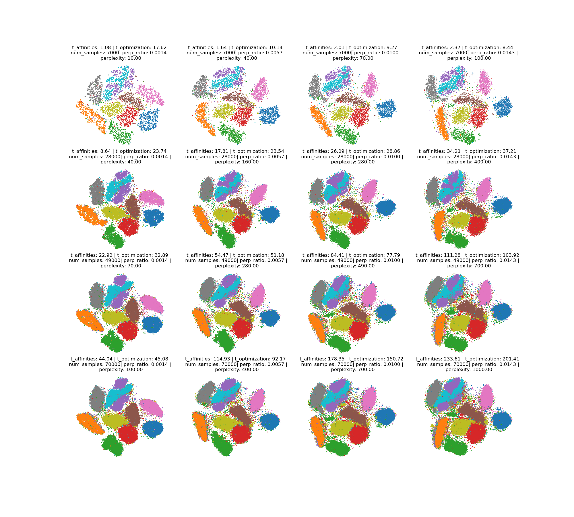
Figure 1: Embeddings of samples of the MNIST data set. From top to bottom, in each column, we increase the number of points, but keep the ratio between perplexity and number of points fixed. From left to right, we increase this ratio. Note that the embeddings are qualitatively stable within each column.

From this experiment, we see that keeping the ratio of perplexity and number of points to be embedded constant, qualitative aspects of the embedding can be transported across different scales.

4.2 Computing embeddings with large perplexity

Previous work showed that the perplexity for a data set is best chosen depending on its size [6, 8]. However, large perplexity values also cause long computation times and easily make applying t-SNE as visualization method infeasible. With the outlined method, we can run an envisioned perplexity on a data set without actually having to compute a full embedding with that perplexity. Consider the results shown in Figure 1. In the bottom right corner, the embedding is computed with ${\operatorname{Perp}=1,000}$. However, the same result can be obtained by embedding a ${\rho=10\%}$ sampling with ${\operatorname{Perp}^{\prime}=100}$ (see upper right corner) and then prolongating it to the fine data set. Then only the smoothing steps need to be computed on the fine data, then, which can be performed with a significantly smaller perplexity, as discussed in the next section. Thereby, the method allows for previous unattainable perplexity values.

4.3 Sensitivity of the embedding to perplexity reduces on finer levels

The approach of embedding a coarse sampling is different from the downsampling approaches previously suggested [8]. That is because, based on the linear relation between perplexity and the number of sample points, we choose corresponding values for perplexity to aim for a certain value at the fine level. It would be natural to assume that value for the smoothing step on the fine prolongated embedding, which might be quite large and thus make smoothing very costly. Indeed, previous work suggests a uniform perplexity of 30 on the fine level, independent of the size of the set of points or the envisioned perplexity [8].

Why is it possible to choose a comparably low perplexity in this step? Our experiments show that the general global structure of the embedding is already fixed after prolongating from the coarse embedding. The smoothing steps after prolongation, therefore, have rather cosmetic effects. Consider the results presented in Figure 2. On the left is an embedding of a coarse sampling of 10% of the points of the MNIST data set. On the right, there are four prolongations from this embedding, computed by respective affinity matrices depending on four perplexities ${(140,70,7,5)}$. The general structure of the smoothed embeddings is unaffected by the choice of perplexity. Even the effect on the Kullback-Leibler divergence is negligible, although it is slightly lower for higher perplexities (we compute the divergence based on a single affinity matrix for comparison, not based on the respective affinity matrices). Qualitatively, the clusters are slightly better separated for higher perplexities.

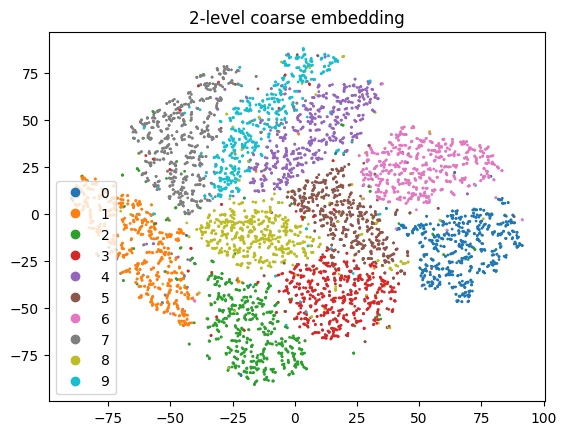
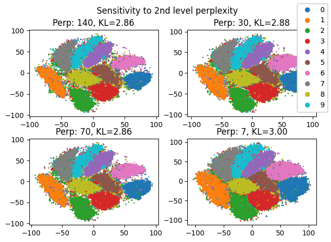
Figure 2: Caption

4.4 Two-level approach gains speed and better NN-preservation

In particular for large data sets, as produced by state-of-the-art single cell transcriptomics pipelines, that contain millions of points, computing an embedding is a lengthy process, even with optimized software such as fit-SNE [10]. While there are fast methods parallel methods available for the GPU [16, 17], these require corresponding hardware and are limited in the size of the data to be processed as that needs to fit the graphic card’s memory. Hence, it is desirable to have a fast embedding method for large data sets that runs on the CPU.

The approach outlined above has the potential to achieve just this. Instead of embedding the full data set, we only embed a small sample set, which reduces computational costs. Only the smoothing steps are run on the fine data set, but these are few compared to the steps necessary to obtain the initial embedding of the coarse data set. Therefore, depending on the sampling rate, about an order of magnitude can be gained in computing the embedding.

In order to quantify the local quality of our embeddings, we turn to the precision/recall metric. For that, we fix a maximum neighborhood size $k_{\max}$. Then, for each ${k\in\{1,\ldots,k_{\max}\}}$, we compute the number of true positives as

$${\operatorname{TP}_{k}=N_{k_{\max}}(X)\cap N_{K}(Y)},$$

that is, the points that are in the high-dimensional neighborhood and also in the low-dimensional embedded neighborhood. From this value we obtain the precision as

$${\operatorname{PR}_{k}=|\operatorname{TP}_{k}|/k}$$

and the recall as

$${\operatorname{RC}_{k}=|\operatorname{TP}_{k}|/k_{\max}}.$$

That is, ideally, the precision is always $1$, while the recall grows as ${k/k_{\max}}$. In the precision/recall diagram, an ideal behavior would thus be a vertical line of measurements sitting at precision $1$ and growing up to recall $1$. See results of the precision/recall for the MNIST data set in Figure 3, which show that our sampling-based approach achieves better neighborhood preservation than base-line t-SNE.

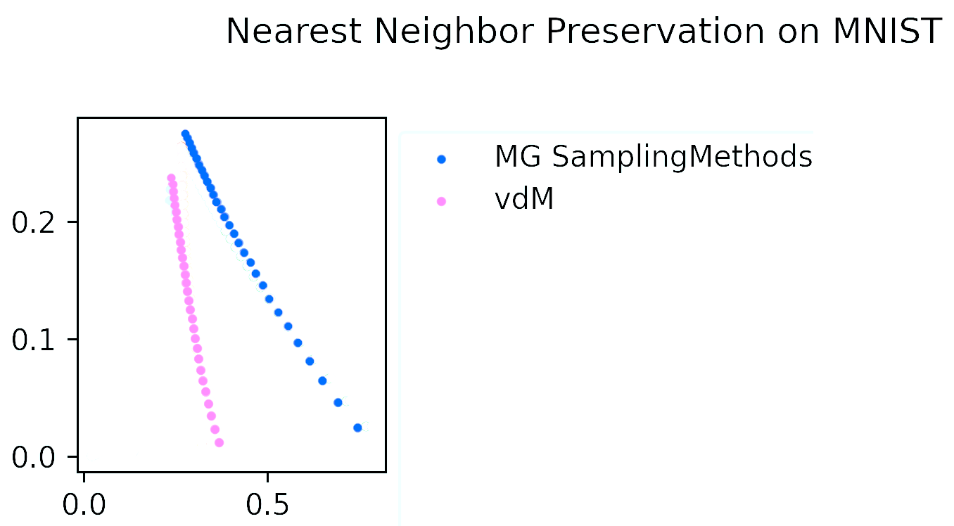
Figure 3: Precision/Recall diagram for the MNIST data set. Note that our sampling-based approach achieves better neighborhood preservation than base-line t-SNE.

5 Discussion

In this paper, we apply a sampling-based approach to the computation of t-SNE embeddings. We show that there is a linear relationship between perplexity values and the size of the data set to be embedded. This key observation allows us to embed data sets with perplexities that are larger than those currently available with state-of-the-art methods. Furthermore, it leads to a scheme that allows for faster embeddings, which even perform better in terms of nearest-neighbor preservation. We thus improve on the sketch of a corresponding method as given in previous work [8].

Several question remain open and are left for future work:

• What happens if the coarse embedding does not reflect the global structure correctly?

• How does our approach relate to HSNE [18]? The two approaches follow different goals, but can they be combined?

• Can the approach be translated to UMAP, despite the fact that it uses stochastic gradient descent?

• What other aspects can be translated from the realm of multigrid solvers, e.g., more levels (despite that our preliminary experiments show no additional gain), different cycles (not V-, but possibly W-, or F-cycles), other sampling or prolongation strategies, as discussed in previous work [8].

Data availability

All data were downloaded following links in the original publications. The MNIST data set is available at https://yann.lecun.com/exdb/mnist/.

References

- [1] Etienne Becht et al. “Dimensionality reduction for visualizing single-cell data using UMAP” In Nature Biotechnology 37.1, 2019, pp. 38–44 DOI: 10.1038/nbt.4314
- [2] Anna C Belkina et al. “Automated optimized parameters for T-distributed stochastic neighbor embedding improve visualization and analysis of large datasets” In Nature communications 10.1 Nature Publishing Group, 2019, pp. 1–12
- [3] Jan Niklas Böhm, Philipp Berens and Dmitry Kobak “Attraction-repulsion spectrum in neighbor embeddings” In The Journal of Machine Learning Research 23.1, 2022, pp. 95:4118–95:4149
- [4] Chao Chen et al. “A robust hierarchical solver for ill-conditioned systems with applications to ice sheet modeling” In Journal of Computational Physics 396 Elsevier, 2019, pp. 819–836
- [5] Sebastian Damrich, Niklas Böhm, Fred A. Hamprecht and Dmitry Kobak “From $t$-SNE to UMAP with contrastive learning” URL: https://openreview.net/forum?id=B8a1FcY0vi
- [6] Jiarui Ding, Anne Condon and Sohrab P Shah “Interpretable dimensionality reduction of single cell transcriptome data with deep generative models” In Nature communications 9.1 Nature Publishing Group, 2018, pp. 1–13
- [7] David Haussler and Emo Welzl “Epsilon-nets and simplex range queries” In Proceedings of the second annual symposium on Computational geometry, 1986, pp. 61–71
- [8] Dmitry Kobak and Philipp Berens “The art of using t-SNE for single-cell transcriptomics” In Nature communications 10.1 Nature Publishing Group, 2019, pp. 1–14
- [9] Dmitry Kobak and George C. Linderman “Initialization is critical for preserving global data structure in both t-SNE and UMAP” In Nature Biotechnology 39.2, 2021, pp. 156–157 DOI: 10.1038/s41587-020-00809-z
- [10] George C. Linderman et al. “Fast interpolation-based t-SNE for improved visualization of single-cell RNA-seq data” In Nature Methods 16.3, 2019, pp. 243–245 DOI: 10.1038/s41592-018-0308-4
- [11] Oren E Livne and Achi Brandt “Lean algebraic multigrid (LAMG): Fast graph Laplacian linear solver” In SIAM Journal on Scientific Computing 34.4 SIAM, 2012, pp. B499–B522
- [12] Laurens van der Maaten and Geoffrey Hinton “Visualizing Data using t-SNE” In Journal of Machine Learning Research 9.86, 2008, pp. 2579–2605 URL: http://jmlr.org/papers/v9/vandermaaten08a.html
- [13] Leland McInnes, John Healy and James Melville “UMAP: Uniform Manifold Approximation and Projection for Dimension Reduction” arXiv, 2020 DOI: 10.48550/arXiv.1802.03426
- [14] Arne Nägel and Gabriel Wittum “Scalability of a parallel monolithic multilevel solver for poroelasticity” In High Performance Computing in Science and Engineering’18: Transactions of the High Performance Computing Center, Stuttgart (HLRS) 2018, 2019, pp. 427–437 Springer
- [15] Simona Perotto, A Reali, P Rusconi and Alessandro Veneziani “HIGAMod: A Hierarchical IsoGeometric Approach for MODel reduction in curved pipes” In Computers & Fluids 142 Elsevier, 2017, pp. 21–29
- [16] Nicola Pezzotti et al. “GPGPU Linear Complexity t-SNE Optimization” In IEEE Transactions on Visualization and Computer Graphics 26.1, 2020, pp. 1172–1181 DOI: 10.1109/TVCG.2019.2934307
- [17] Mark Ruit, Markus Billeter and Elmar Eisemann “An Efficient Dual-Hierarchy t-SNE Minimization” In IEEE Transactions on Visualization and Computer Graphics 28.1, 2022, pp. 614–622 DOI: 10.1109/TVCG.2021.3114817
- [18] Vincent Unen et al. “Visual analysis of mass cytometry data by hierarchical stochastic neighbour embedding reveals rare cell types” In Nature Communications 8.1, 2017, pp. 1740 DOI: 10.1038/s41467-017-01689-9
- [19] Laurens Van Der Maaten “Accelerating t-SNE using tree-based algorithms” In The Journal of Machine Learning Research 15.1, 2014, pp. 3221–3245
- [20] Martin Wattenberg, Fernanda Viégas and Ian Johnson “How to use t-SNE effectively” In Distill 1.10, 2016, pp. e2