Observing hidden neuronal states in experiments

Abstract

We construct systematically experimental steady-state bifurcation diagrams for entorhinal cortex neurons. A slowly ramped voltage-clamp electrophysiology protocol serves as closed-loop feedback controlled experiment for the subsequent current-clamp open-loop protocol on the same cell. In this way, the voltage-clamped experiment determines dynamically stable and unstable (hidden) steady states of the current-clamp experiment. The transitions between observable steady states and observable spiking states in the current-clamp experiment reveal stability and bifurcations of the steady states, completing the steady-state bifurcation diagram.

Introduction.–

When characterising the dynamics of nonlinear systems, one fundamental criterion for a model is if its invariants such as steady states or periodic orbits match experimental observations. The ability to validate models is, thus, greatly expanded by experimental tools with the capacity to unveil non-observable (sensitive or dynamically unstable) invariant states that are otherwise inaccessible to standard measurements. This letter applies the experimental technique to use feedback control for tracking unstable states while varying parameters to electrophysiology experiments on neuronal cells. Our aim is to support systematic validation of neuron models by comparing bifurcation diagrams and observing their between-cells variability. We focus on unstable parts of steady-state branches obtained by feedback-controlled experiments and compare them with indirect evidence from standard measurements from open-loop experiments. This extends recent work of Ori et al. [1, 2] constructing phase diagrams from neuronal data, and complements other approaches such as using data to verify the bifurcation structure of neuronal models [3, 4], model-based data analysis [5] or parameter estimation from data [6]. Our approach is similar to recent experimental demonstrations in mechanical systems [7], vibrations and buckling experiments [8, 9], pedestrian flow experiments [10], cylindrical pipe flow simulations [11] and feasibility studies for synthetic gene networks [12, 13].

In our electrophysiology experiments on entorhinal cortex neurons we apply a voltage clamp (VC) [14, 15], followed by current clamp (CC). In the VC setup the electrode acts as a voltage source, fixing the potential across the neural membrane, measuring the current, while the CC setup adds a fixed external current, measuring the resulting membrane potential (see Fig. 1(a)). The VC experiment is the closed-loop feedback-controlled part of the protocol and CC is the open-loop protocol, because in-vivo neurons are subject to current signals that drive spiking (oscillatory) or rest (steady) states of the neural membrane potential. VC has been applied successfully to study neuronal nonlinear current-voltage relationships, so-called N-shaped $I$-$V$ characteristics, which cause enhanced neuronal excitability and influence the regenerative activation of certain ionic currents (e.g., sodium) [16, 17, 18, 19, 20] across the neural membrane, into and out of the cell. We show that the VC protocol with a slowly varied reference voltage signal gives access to stable and unstable neuronal steady states of the neuron. In contrast, the open loop CC protocol with a slowly varying applied current always follows stable (observable) states, driving the neuron to dynamically transition between its observable rest states and its observable spiking states.

We interpret these combined experimental protocols (VC and CC) using multiple-timescale dynamics, in particular, the dissection method [21], which reveals the dynamic bifurcations in the experiment; see Fig. 1(b).

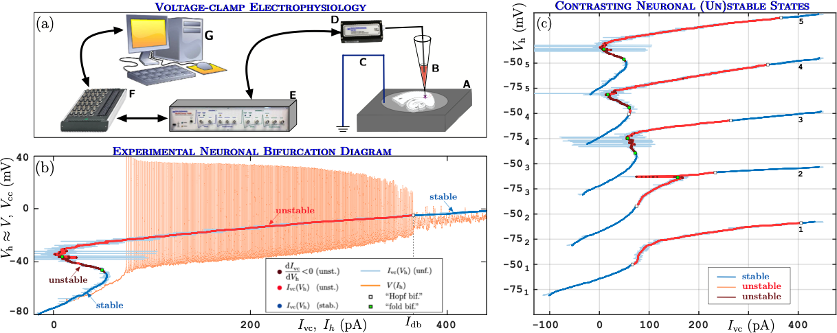
Figure 1: (a) Experimental setup with brain slice (A), patch pipette (B), reference electrode ((Ag-AgCl pellet) connected to ground (C), amplifier (E, Multiclamp 700B) with CV-7B headstage (D), AD-converter (F, National Instruments NI USB-6343) and standard PC computer (G). (b) VC and CC protocol runs for cell $5$: $(I_{\mathrm{vc}}(t),V_{\mathrm{h}}(t))$-curve for VC run (thin bright blue: unfiltered data with sampling time step $5\times 10^{-5}$ s, blue/red/brown: median of $I_{\mathrm{vc}}$ over moving windows of size $\Delta w=4\times 10^{3}$ steps equalling $0.2$s) and $(I_{\mathrm{h}}(t),V_{\mathrm{cc}}(t))$-curve for CC run (orange, mean of $I_{\mathrm{h}}$ over moving windows. (c) $(I_{\mathrm{vc}}(t),V_{\mathrm{h}}(t))$-curves for VC protocol of all $5$ cells on waterfall $V_{\mathrm{h}}$-axis (same color coding as (b)).

In this slow-fast framework, the states traced by the VC protocol with slow variation correspond to the steady-state experimental bifurcation diagram of the so-called fast subsystem of mathematical model describing the protocol [21]. Hence, the N-shaped I-V relation of a neuron should be seen as a S-shaped V-I bifurcation diagram; see again Fig. 1(b).
Following this strategy, we demonstrate the feasibility of tracking a family of neuronal steady states (stable and unstable) via variations of reference signal and reparameterizing the obtained curve using the feedback current.

Protocol.–

We applied first VC and then CC protocol to $5$ neurons in the entorhinal cortex of $4$ male Wistar rats [22]. We first performed the VC neuronal recordings varying the hold voltage $V_{\mathrm{h}}$ from $-80$ mV to $+30$ mV slowly with $\dot{V}_{\mathrm{h}}=1.83$ mV​$/$s, while measuring current, called $I_{\mathrm{vc}}$ in Fig. 1(b,c). Subsequently, for the CC recordings we first determine the minimal injected current required to induce a depolarization block of action potential generation ($I_{\mathrm{db}}$ in Fig. 1(b), upper limit of current input where firing occurs). Then we gradually increased the injected current from $0$ pA to $I_{\mathrm{db}}$ during $60$ s, such that $\dot{I}_{\mathrm{h}}$ is in the range $6.6\ldots 7.4$ pA$/$s for the $5$ neurons, while recording voltage $V_{\mathrm{cc}}(t)$. See SM for full description and further checks (e.g., for hysteresis).

Results.–

Figure 1(b) shows the time profiles $(I_{\mathrm{h}}(t),V_{\mathrm{cc}}(t))$ of the CC protocol run (orange, thin) and $(I_{\mathrm{vc}}(t),V_{\mathrm{h}}(t))$ of the VC protocol run (bright blue, thin) for cell $5$ overlaid in the $(I,V)$-plane. After smoothing the VC time profile is the S-shaped curve $(I_{\mathrm{vc,sm}}(V_{\mathrm{h}}),V_{\mathrm{h}})$ (blue/brown/red, thick). It equals the $(I,V)$-characteristic of the stationary neuronal states of the CC protocol, including dynamically unstable states (brown and red). The transition to stable spiking states is compatible with type-I excitability, however we do not have sufficient data to conclude; see SM, Fig. S2. Their dynamical instability is inferred in two ways: (i) by the negative slope of the $(I_{\mathrm{vc,sm}},V_{\mathrm{h}})$-curve (brown) after smoothing over a moving window with larger size $\Delta w=1.5\times 10^{4}$ steps ($=0.75$s), or (ii) by the presence of oscillations (neuronal firing) in the CC run at $I_{\mathrm{h}}$ equalling the $I_{\mathrm{vc,sm}}$ (red). The stability boundaries of the stationary states are labelled as bifurcations in Fig. 1(b). The change of stability near the disappearance of stable spiking states at $I_{\mathrm{db}}$ is a Hopf bifurcation. The fold points of the $(I_{\mathrm{vc,sm}},V_{\mathrm{h}})$-curve are saddle-node (fold) bifurcations. Figure 1(c) shows the stationary-state curves with their inferred dynamical stability for all $5$ cells (see SM for CC run time profiles used to partially infer stability of cells $1$–$4$). The cells are vertically ordered and numbered according to depth of the S-shape, determining if they fall into the class of type-I or type-II neurons. Figure 1(c) demonstrates wide variability in steady-state curve shape among cells of nominally same function.

Analysis.–

To see why VC-run time profiles approximate the experimental bifurcation diagram with unstable stationary states of neurons in CC protocol, we use the formalism of multiple-timescale dynamical systems. Superimposing the data from VC and CC protocol also gives the first experimental illustration of slow-fast dissection. The effect of the respective clamps can be understood in a general conductance-based model for the neuron,

$$C\dot{V} =-\textstyle{\sum}_{j}I_{j}(x_{j},V)+I_{\mathrm{ext}}, \dot{x}_{j} =\frac{x_{\infty,j}(V)-x_{j}}{\tau_{j}(V)},$$ (1)

describing the current balance across the neuron’s membrane. The membrane potential is $V$, $I_{j}(x_{j},V)_{j=1,\ldots,N}$ are the currents across different voltage-gated ion channel types and $I_{\mathrm{ext}}$ is the external current. Each ionic channel type $j$ has an associated gating variable $x_{j}$ with steady-state gating function $x_{\infty,j}(V)$ and relaxation time $\tau_{j}(V)$. The observed dynamic effects such as oscillations (firing/spiking) and negative-slope $(I,V)$ characteristics are determined by these channel coefficients $I_{j}$, $x_{\infty,j}$ and $\tau_{j}$ that are traditionally obtained by parameter fitting from VC experiments, a difficult and mostly ill-posed problem [23].

The VC and CC protocols use different mechanisms for generating $I_{\mathrm{ext}}(t)$. The VC protocol is a closed loop where a voltage source regulates $I_{\mathrm{ext}}$ with high gain $g_{\mathrm{c}}$ to achieve the slowly varying hold voltage $V_{\mathrm{h}}$ at the voltage source for (1), measuring $I_{\mathrm{vc}}$:

$$I_{\mathrm{ext}} \approx I_{\mathrm{vc}}=g_{\mathrm{c}}(V_{\mathrm{h}}-V), \dot{V}_{\mathrm{h}} =\varepsilon\Delta_{V}$$ (2)

which turns (1), (2) into a multiple-timescale dynamical system with $N+1$ fast state variables $(V,x_{j})$ and one slow state variable $V_{\mathrm{h}}$, corresponding to the feedback reference signal [24]. The speed at which $V_{\mathrm{h}}$ varies is $\varepsilon\Delta_{V}$ with $\Delta_{V}(t)=0.183$ mV​$/$ms, where we extract the dimensionless small factor $\varepsilon=10^{-2}$.

In contrast, the CC protocol holds $I_{\mathrm{ext}}$, measuring the generated voltage $V_{\mathrm{cc}}$, thus, corresponding to an open-loop system, permitting e.g. the spiking seen in Fig. 1(b):

$$I_{\mathrm{ext}} \approx I_{\mathrm{h}}, V_{\mathrm{cc}} \approx V, \dot{I}_{\mathrm{h}} =\varepsilon\Delta_{I}.$$ (3)

The applied hold current $I_{\mathrm{h}}$ is varied slowly at speed $\varepsilon\Delta_{I}$ with $\varepsilon=10^{-2}$ and $\Delta_{I}=0.66\ldots 0.75$ pA$/$ms. System (1), (3) is also a slow-fast system with $1+N$ fast variables $(V,x_{j})$ and $1$ slow variable $I_{\mathrm{h}}$. The gain $g_{\mathrm{c}}$ in (2) is limited by the imperfect conductance across the non-zero spatial extent of the membrane. Even though (1) is for the potential $V$ across the entire membrane and only $V_{\mathrm{h}}$ at the clamp is measured, we approximate $V_{\mathrm{h}},V_{\mathrm{cc}}\approx V$ for, the membrane potential, and $I_{\mathrm{h}},I_{\mathrm{vc}}\approx I_{\mathrm{ext}}$ for the external current in (1).

Following a classical multiple-timescale approach, we consider the $\varepsilon=0$ limit of system (1), (2), which corresponds to its $(1+N)$-dimensional fast subsystem (1) with $I_{\mathrm{ext}}=g_{\mathrm{c}}(V_{\mathrm{h}}-V)$, where $V_{\mathrm{h}}$ is now treated as a parameter. For fixed $V_{\mathrm{h}}$ and voltages in the range $-80\ldots 30$ mV of interest, system (1) has only stable steady states (no limit cycles, that is, no neuronal spikes); see SM for details. For a fixed hold voltage $V_{\mathrm{h}}$, the steady states of model (1) with $I_{\mathrm{ext}}=g_{\mathrm{c}}(V_{\mathrm{h}}-V)$ satisfy the algebraic equations for $(V,x_{j})_{j=1,\ldots,N}$

$$\textstyle{\sum_{j}}I_{j}(x_{j},V) =g_{\mathrm{c}}(V_{\mathrm{h}}-V), x_{j}=x_{\infty,j}(V),$$ (4)

where $I_{\mathrm{eq}}(V)=\sum_{j}I_{j}(x_{\infty,j},V)$ is the equilibrium current for fixed membrane potential $V$. The solutions of (4) form a (1D) steady-state curve of system (1), (2), which is normally hyperbolic (transversally attracting) for $\varepsilon=0$. For $\varepsilon\neq 0$ the increase of $V_{\mathrm{h}}$ with speed $\varepsilon\Delta_{V}$ introduces a slow variation of all states $(V,x_{j})$. Hence, $V$ and the feedback current $I_{\mathrm{vc}}=g_{\mathrm{c}}(V_{\mathrm{h}}-V)$ (as measured), are not at their steady-state values given by (4), but they are changing dynamically. This results in a difference between the measured curve $(I_{\mathrm{vc}},V_{\mathrm{h}})$ in Figure 1(b) and the $(I,V)$-values of the desired steady-state curve (4).

Figure 2: VC and CC in silico. Protocol as described for Fig. 1 applied to a type-I Morris-Lecar neuron model [25]; see SM for parameter values. The two-dimensional fast subsystem has a S-shaped steady-state curve satisfying(4). The steady-state curve (4) and the (multi-color) S-shaped curve from the VC protocol indistinguishable throughout the range of input currents $I_{\mathrm{vc}}$. The orange curve resulting from the CC protocol is very close to $S^{0}$ and the VC protocol near its dynamically stable parts.

Geometrical singular perturbation theory (GSPT) by Fenichel [26] implies that after decay of initial transients every trajectory of the VC protocol modelled by system (1), (2) satisfies equation (4) for the steady-state curve up to order $\varepsilon$. The first-order terms in $\varepsilon$ are

$$I_{\mathrm{eq}}(V)-I_{\mathrm{vc}}(V) \approx I_{\mathrm{eq}}^{\prime}(V)\dot{V}\,\frac{\tau_{1/2}}{\ln 2}\lesssim I_{\mathrm{eq}}^{\prime}(V_{\mathrm{h}})0.2\mbox{\,mV},$$ (5)

where $\tau_{1/2}$ is the time for deviations from the transversally stable steady-state curve (4) to decay to half of their initial value; see SM for details (equation (S13) and Fig. S3). We estimate $\tau_{1/2}$ from recovery transients after disturbances naturally occuring from imperfections in the voltage clamp during VC runs as $\tau_{1/2}\lesssim 0.075$ s (see SM, Fig. S3(b)), such that $\dot{V}\tau_{1/2}/\ln 2\approx\dot{V}_{\mathrm{h}}\tau_{1/2}/\ln 2\lesssim 0.2$ mV. Thus, the systematic bias between $I_{\mathrm{vc,sm}}(V_{\mathrm{h}})$ in Fig. 1(b) and the true steady state curve $I_{\mathrm{eq}}(V)$ caused by dynamically changing $V_{\mathrm{h}}$ is below measurement disturbances.

Estimate (5) can also be tested in silico. Figure 2 emulates both VC and CC protocols with the Morris-Lecar model [25], which is of the form (1) with $j=1$. For the chosen parameter set (see SM), the curves $(I_{\mathrm{vc}}(t),V_{\mathrm{h}}(t))$ and $(I_{\mathrm{eq}}(V_{\mathrm{h}}(t)),V_{\mathrm{h}}(t))$ are order $\varepsilon$ ($\approx 1$%) apart.

Consequently, time profile $(I_{\mathrm{vc}}(t),V_{\mathrm{h}}(t))$ follows closely the curve (4) of stable steady states of the fast subsystem (1) with VC protocol $I_{\mathrm{ext}}=g_{\mathrm{c}}(V_{\mathrm{h}}-V)$, treating $V_{\mathrm{h}}$ as a parameter. We now connect the curve (4) to a curve of fast-subsystem equilibria of the CC protocol, which is in part unstable. To this end we recast the VC protocol in the form of a CC protocol with non-constant current ramp speed $\varepsilon\Delta_{I,\mathrm{vc}}(t)$ and disturbances: the smoothed time profile $I_{\mathrm{vc,sm}}(V_{\mathrm{h}}(t))$ in Fig. 1(b) of the VC run (thick, in blue/brown/red) equals the raw-data measured time profile $I_{\mathrm{vc}}(t)$ (thin blue curve with fluctuations) plus disturbances $\eta_{\mathrm{vc}}(t)$, defined by $\eta_{\mathrm{vc}}(t)=I_{\mathrm{vc,sm}}(V_{\mathrm{h}}(t))-I_{\mathrm{vc}}(t)$. After smoothing, the derivative $I_{\mathrm{vc,sm}}^{\prime}(V_{\mathrm{h}})$ w.r.t. $V_{\mathrm{h}}$ is moderate ($\lesssim 20$ pA$/$mV in modulus at its maximum near $I_{\mathrm{db}}$), such that the VC protocol implies

$$I_{\mathrm{ext}}\approx I_{\mathrm{vc,sm}}+\eta_{\mathrm{vc}},\ \dot{I}_{\mathrm{vc,sm}}=\varepsilon\Delta_{I,\mathrm{vc}}(t),$$ (6)

where $\Delta_{I,\mathrm{vc}}(t)=I_{\mathrm{vc,sm}}^{\prime}(V_{\mathrm{h}}(t))\Delta_{V}\approx I_{\mathrm{eq}}^{\prime}(V_{\mathrm{h}}(t))\Delta_{V}$ with upper bound $\max_{t}|\Delta_{I,\mathrm{vc}}(t)|\lesssim 3.7$ pA$/$ms in the range of Fig. 1(b). Thus, $I_{\mathrm{vc,sm}}$ is indeed still slow. Hence, except for disturbances $\eta_{\mathrm{vc}}(t)$, the external current $I_{\mathrm{ext}}$ is slowly varying according to a CC protocol with slowly time-varying speed $\varepsilon\Delta_{I,\mathrm{vc}}(t)$, such that the VC protocol (2) is equivalent CC protocol (6) with disturbances $\eta_{\mathrm{vc}}$.

Systems (1), (3) and (1), (6) without disturbances ($\eta_{\mathrm{vc}}=0$) are both models of CC protocols. They have the same fast subsystem (1) when setting $\varepsilon=0$ and identifying $I_{\mathrm{h}}$ and $I_{\mathrm{vc,sm}}$. The respective fast-subsystem steady states $(V,x_{j})_{j=1,\ldots,N}$ satisfy

$$\textstyle{\sum_{j}}I_{j}(x_{j},V) =I_{\mathrm{h}}(=I_{\mathrm{vc,sm}}), x_{j}=x_{\infty,j}(V).$$ (7)

However, systems (1), (3) and (1), (6) differ by the nature of their respective slow variables $I_{\mathrm{h}}$ and $I_{\mathrm{vc,sm}}$: $I_{\mathrm{h}}$ is an externally applied hold current for (3), while $I_{\mathrm{vc,sm}}$ is a measured (and smoothed) current from the feedback control $g_{\mathrm{c}}(V_{\mathrm{h}}-V)$ of the voltage source for (6). Thus, while the S-shaped steady-state curve $(I_{\mathrm{eq}}(V),V)$ is identical for both systems, it contains large unstable segments as a steady-state curve of (1), (3), while it always stable as a steady-state curve of (1), (6). The change in stability is caused by the disturbances $\eta_{\mathrm{vc}}$, which are current adjustments generated by the feedback term in (2), $I_{\mathrm{vc}}=g_{\mathrm{c}}(V_{\mathrm{h}}-V)$. Along most of the curve $(I_{\mathrm{vc,sm}}(V_{\mathrm{h}}),V_{\mathrm{h}})$ the $\eta_{\mathrm{vc}}$ are small fluctuations such that $I_{\mathrm{vc,sm}}(V_{\mathrm{h}})\approx I_{\mathrm{vc}}(V_{\mathrm{h}})$ and the feedback is approximately non-invasive [7]. Estimate (5) ensures that the measurements $I_{\mathrm{vc}}(V)$ stay close to $I_{\mathrm{eq}}(V)$. Therefore, we can conclude that the VC protocol (2) with slowly varying feedback reference signal $V_{\mathrm{h}}$ reveals the entire family of steady states of a neuron (type 1 or 2) with constant external current $I_{\mathrm{ext}}$, both stable (observable) and unstable (non-observable, hidden). Consequently, the N-shaped $I$-$V$ relations for type-1 neurons reported in [16, 17, 20] equal S-shaped steady-state bifurcation diagrams for these neurons with respect to $I_{\mathrm{ext}}$. They are tractable with a VC protocol where the current $I_{\mathrm{ext}}$ is a sufficiently slowly varying feedback current with sufficiently small fluctuations $\eta_{\mathrm{vc}}$. In particular, this allows us to detect and pass through fold bifurcations directly in the experiment.

In contrast, for the CC open-loop protocol (3) applying a slowly varying electrical current the neuron dynamically transitions between its observable rest states and its observable (dynamically stable) spiking states (see Fig. 1(b) orange timeprofile). The speed of variation $\varepsilon\Delta_{I}\lesssim 0.75\times 10^{-3}$ pA$/$ms is such that $I_{\mathrm{ext}}$ varies by only about $1$ pA per spiking period. Transients to step current responses in the stable spiking region have a half-time for decay $\tau_{1/2}\lesssim 0.2$ s (see SM, Fig. S5 for the response to a step to $I_{\mathrm{ext}}=200$ pA), permitting us to estimate the systematic bias between true steady-state spiking and the response to dynamically changing $I_{\mathrm{ext}}$, similar to (5) for certain features of the periodic spike train. For example, the bias in the spike minimum $V_{\mathrm{min}}$ near $I_{\mathrm{h}}=200$ mA is $V_{\mathrm{min}}^{\prime}(I_{\mathrm{h}})\times\dot{I}_{\mathrm{h}}\times\tau_{1/2}/\ln 2\sim 0.14$ mV to first order of $\varepsilon$. Near the approximate Hopf bifurcation at $I_{\mathrm{h}}\approx I_{\mathrm{db}}$ in the experiment the bias will exceed order $\epsilon$ as both, $\tau_{1/2}$ and $V_{\mathrm{min}}^{\prime}(I_{\mathrm{h}})$ approach infinity at Hopf bifurcations. Thus, combining VC protocol, recast as (6) varying $I_{\mathrm{vc,sm}}$, and the CC protocol (3), varying $I_{\mathrm{h}}$, enables us to interpret the data sets from both protocols in Fig. 1(b) as a bifurcation diagram including unstable states.

For the experimental curves presented in Fig. 1(b,c) (and also in Fig. S1), the disturbances $\eta_{\mathrm{vc}}$ are not small in some unstable parts of the reported steady-state curve (e.g., near $V_{\mathrm{h}}=-30$ mV in Fig. 1(b)), caused by imperfect voltage clamping across the membrane (see Fig. S3(b) in SM for a zoom into these intermittent dropout events). Furthermore, the distances between $(I_{\mathrm{vc,sm}}(t),V_{\mathrm{h}}(t))$ in the VC run and $(I_{\mathrm{h}}(t),V_{\mathrm{cc}}(t))$ in the CC run for the same cell are visibly larger along parts of the curve corresponding to dynamically stable stationary states. This is due to the natural drift of the neuron’s physiological properties as it changes dynamically from one protocol to the other.

Outlook.–

Tracking non-observable (hidden) states through their stability boundaries in experimental settings bridges the gap between real-world phenomena and nonlinear science. Specifically, closed-loop control methods with slow variations of feedback reference signals enable us to discover unstable underlying states of nonlinear systems. Future work will focus on employing fully dynamic clamp electrophysiology [27, 28, 29, 2], which involves two-way real-time communication between neuronal tissue and computer control, permitting non-invasive feedback control with complex reference signals. This will allow biologists to validate computational models by comparing their numerical bifurcation diagrams with experimental ones in parameter regions where the uncontrolled spiking response is dynamically unstable or sensitive with respect to system parameters.

References

- Ori et al. [2018] H. Ori, E. Marder, and S. Marom, Proc. Natl. Acad. Sci. USA 115, E8211 (2018).
- Ori et al. [2020] H. Ori, H. Hazan, E. Marder, and S. Marom, Proc. Natl. Acad. Sci. USA 117, 3575 (2020).
- Levenstein et al. [2019] D. Levenstein, G. Buzsáki, and J. Rinzel, Nat. Commun. 10, 2478 (2019).
- Hesse et al. [2022] J. Hesse, J.-H. Schleimer, N. Maier, D. Schmitz, and S. Schreiber, Nat. Commun. 13, 3934 (2022).
- Sip et al. [2023] V. Sip, M. Hashemi, T. Dickscheid, K. Amunts, S. Petkoski, and V. Jirsa, Sci. Adv. 9, eabq7547 (2023).
- Ladenbauer et al. [2019] J. Ladenbauer, S. McKenzie, D. F. English, O. Hagens, and S. Ostojic, Nat. Commun. 10, 4933 (2019).
- Sieber et al. [2008] J. Sieber, A. Gonzalez-Buelga, S. A. Neild, D. J. Wagg, and B. Krauskopf, Phys. Rev. Lett. 100, 244101 (2008).
- Renson et al. [2019] L. Renson, A. Shaw, D. Barton, and S. Neild, Mech. Syst. Signal Process. 120, 449 (2019).
- Neville et al. [2018] R. M. Neville, R. M. J. Groh, A. Pirrera, and M. Schenk, Phys. Rev. Lett. 120, 254101 (2018).
- Panagiotopoulos et al. [2022] I. Panagiotopoulos, J. Starke, and W. Just, Phys. Rev. Res. 4, 043190 (2022).
- Willis et al. [2017] A. P. Willis, Y. Duguet, O. Omelchenko, and M. Wolfrum, J. Fluid Mech. 831, 579–591 (2017).
- de Cesare et al. [2022] I. de Cesare, D. Salzano, M. di Bernardo, L. Renson, and L. Marucci, ACS Synth. Biol. 11, 2300 (2022).
- Blyth et al. [2023] M. Blyth, K. Tsaneva-Atanasova, L. Marucci, and L. Renson, Nonlinear Dynam. 111, 7975 (2023).
- Cole [1955] K. S. Cole, in Electrochemistry in biology and medicine, edited by T. Shedlovsky (1955) p. 121.
- Hodgkin and Huxley [1952] A. L. Hodgkin and A. F. Huxley, J. Physiol. 117, 500 (1952).
- Schwindt and Crill [1981] P. Schwindt and W. Crill, Brain Res. 207, 471 (1981).
- Fishman and Macey [1969] H. M. Fishman and R. I. Macey, Biophys. J. 9, 151 (1969).
- Johnston et al. [1980] D. Johnston, J. J. Hablitz, and W. A. Wilson, Nature 286, 391 (1980).
- Blatt [1988] M. R. Blatt, J. Membr. Biol. 102, 235 (1988).
- Vervaeke et al. [2006] K. Vervaeke, H. Hu, L. J. Graham, and J. F. Storm, Neuron 49, 257 (2006).
- Rinzel [1987] J. Rinzel, in Mathematical topics in population biology, morphogenesis and neurosciences (Proceedings of an International Symposium held in Kyoto, November 10-15, 1985), Lect. Notes Biomath., Vol. 71 (Springer, 1987) pp. 267–281.
- Amakhin et al. [2021] D. V. Amakhin, E. B. Soboleva, A. V. Chizhov, and A. V. Zaitsev, Int. J. Mol. Sci. 22, 12174 (2021).
- de Abril et al. [2018] I. M. de Abril, J. Yoshimoto, and K. Doya, Neural Netw. 102, 120 (2018).
- Izhikevich [2007] E. M. Izhikevich, Dynamical Systems in Neuroscience (MIT Press, 2007).
- Morris and Lecar [1981] C. Morris and H. Lecar, Biophys. J. 35, 193 (1981).
- Fenichel [1979] N. Fenichel, J. Differ. Eq. 31, 53 (1979).
- Sharp et al. [1993] A. A. Sharp, M. B. O’Neil, L. F. Abbott, and E. Marder, J. Neurophysiol. 69, 992 (1993).
- Marder et al. [1996] E. Marder, L. F. Abbott, G. G. Turrigiano, Z. Liu, and J. Golowasch, Proc. Natl. Acad. Sci. USA 93, 133481 (1996).
- Chizhov et al. [2014] A. V. Chizhov, E. Malinina, M. Druzin, L. J. Graham, and S. Johansson, Front. Cell. Neurosci. 8, 86 (2014).