Characterizing Learning Curves During Language Model Pre-Training: Learning, Forgetting, and Stability

Abstract

How do language models learn to make predictions during pre-training? To study this question, we extract learning curves from five autoregressive English language model pre-training runs, for 1M tokens in context. We observe that the language models generate short repetitive phrases before learning to generate longer and more coherent text. We quantify the final surprisal, within-run variability, age of acquisition, forgettability, and cross-run variability of learning curves for individual tokens in context. More frequent tokens reach lower final surprisals, exhibit less variability within and across pre-training runs, are learned earlier, and are less likely to be “forgotten” during pre-training. Higher $n$-gram probabilities further accentuate these effects. Independent of the target token, shorter and more frequent contexts correlate with marginally more stable and quickly acquired predictions. Effects of part-of-speech are also small, although nouns tend to be acquired later and less stably than verbs, adverbs, and adjectives. Our work contributes to a better understanding of language model pre-training dynamics and informs the deployment of stable language models in practice.

1 Introduction

Language models have received unprecedented attention in recent years due to impressive performance on natural language tasks (e.g. OpenAI, 2022; Google, 2023). However, these models are initialized as random word (token) generators, and it remains unclear how the models achieve complex linguistic abilities during pre-training. Previous work has investigated when syntactic, semantic, and reasoning abilities emerge (Liu et al., 2021; Evanson et al., 2023) and extracted learning curves for individual examples (Xia et al., 2023), but specific features that influence individual learning curves have yet to be identified. Given any token in context, it is unknown when or how stably that token would be learned by a language model.

Understanding when and how examples are learned by language models has implications for how any agent might acquire language and what behaviors to expect from deployed models. Scientifically, language model learning patterns provide insights into how learning from language statistics alone (i.e. “distributional” learning) can lead to complex linguistic abilities (Mahowald et al., 2023). This has implications for distributional learning mechanisms in people (Chang and Bergen, 2022b; Warstadt and Bowman, 2023). From a practical perspective, understanding language model learning curves would allow NLP practitioners to determine how much pre-training is necessary for different capabilities, what behaviors will remain stable after additional training, and what levels of variability to expect in any fully-trained model.

To quantify learning patterns during language model pre-training, we run five English language model pre-training runs, and we extract learning curves for 1M tokens in context. We quantify the final surprisal, variability within and across pre-training runs, age of acquisition, and forgettability of each example. We report general learning patterns, and we assess the impact of token frequencies, $n$-gram probabilities, context lengths and likelihoods, and part-of-speech tags on the speed and stability of language model learning.

2 Related Work

Previous work has studied the pre-training dynamics of language models (Saphra and Lopez, 2019). Choshen et al. (2022) and Evanson et al. (2023) find that language models learn linguistic generalizations in similar stages regardless of model architecture, initialization, and data-shuffling. In masked language models, syntactic rules are learned early, but world knowledge and reasoning are learned later and less stably (Chiang et al., 2020; Liu et al., 2021). Olsson et al. (2022) find that copy mechanisms (“induction heads” for in-context learning) appear at an inflection point during pre-training. These results establish when a variety of abilities emerge in language models.

Previous work has also studied how individual examples are learned during pre-training. For example, word learning is highly dependent on word frequency (Chang and Bergen, 2022b). Larger models memorize more examples during pre-training without overfitting (Tirumala et al., 2022), but the time step that a model sees an example does not affect memorization (Biderman et al., 2023). Most similar to our work, Xia et al. (2023) collect learning curves for individual tokens in context, finding that some examples exhibit a “double-descent” trend where they first increase then decrease in surprisal. All of the studies above collect language model learning curves during pre-training, either for individual examples or targeted benchmark performance. Here, we introduce metrics to characterize such curves, we identify general learning patterns, and we isolate text features that are predictive of learning speed and stability.

3 Language Model Learning Curves

We extract learning curves for 1M tokens in context from five language model pre-training runs.

3.1 Models and Dataset

We pre-train five autoregressive Transformer language models from scratch, following the GPT-2 architecture with 124M parameters (Radford et al., 2019). We use a SentencePiece tokenizer trained on 10M lines of our pre-training dataset with vocabulary size 50K.

Dataset and training.

We retrieve the first 128M lines of the deduplicated OSCAR English corpus (Abadji et al., 2021). We tokenize the corpus, concatenating lines until each sequence has length 128. We sample $80\%$ of the resulting dataset as our pre-training dataset (5.1B tokens), leaving the remainder for evaluation and testing. Models are trained for 1M steps with batch size 256 (Devlin et al., 2019; Chang and Bergen, 2022b). Each model is initialized with a different random seed and uses a different shuffle of the pre-training dataset. Pre-training details and hyperparameters are in §A.1

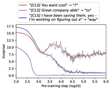
Figure 1: Learning curves for three evaluation examples from the OSCAR dataset during one pre-training run. Colored lines are fitted GAM curves.

Step	Training tokens	Model output
0	0	‘‘This is469 gush liqueur Defense trophies Jakarta Sale Berlin deservingException validate jalapeno...’’
100	3.3M	‘‘This is,,,,,,,,,,,,,,,,,,,,,,,,,,,,,,,, the the the the,,,,,,,......’’
1K	33M	‘‘This is a few of the first of the same of the world’s the most of the first of the the same of the first of the world.’’
10K	330M	‘‘This is a great way to make a difference in your life.’’
100K	3.3B	‘‘This is a very important part of the process of getting your business off the ground.’’
1M	33B	‘‘This is a great opportunity to own a beautiful home in the desirable area of North Vancouver.’’

Table 1: Sample model outputs completing the prompt ‘‘This is...’’ at different pre-training checkpoint steps, using sampling temperature $0.3$. We also report the total number of tokens observed up to a given step; one epoch of our pre-training dataset is 5.1B tokens.

Checkpoints.

Previous work studying language models during pre-training has saved model checkpoints at inconsistent intervals (e.g. every 100 steps or every power of two up to step 1000, then every 1000 steps up to step 100K, etc; Blevins et al., 2022; Chang and Bergen, 2022b; Sellam et al., 2022; Biderman et al., 2023; Xia et al., 2023). To obtain smoother changes between checkpoints, we save checkpoints such that the number of steps between checkpoints increases linearly as a function of the current step $t$. As a result, (1) we can define the checkpoint frequencies at the start and end of pre-training, (2) the checkpoint step is an exponential function of the checkpoint number, and (3) the number of steps per checkpoint is an exponential function of the checkpoint number. Checkpoint strategy details are in §A.2. We begin pre-training with 100 steps per checkpoint, and we end pre-training with 25K steps per checkpoint (ending at step 1M). Including a checkpoint at step zero, this results in 222 checkpoints per pre-training run. Sample outputs from different checkpoints are included in §4.

3.2 Surprisal Curves

For quantitative analyses of language model learning curves, we sample 100K sequences from the evaluation dataset in §3.1. We sample ten tokens per sequence, and we compute the surprisal $-\text{log}_{2}(P(w))$ for each token $w$ based on its preceding context (Levy, 2008), using each language model checkpoint. This results in a learning curve for each token in context (i.e. each example) and each model, usually trending from higher surprisal (worse predictions) to lower surprisal (better predictions; Figure 1). Surprisal is equivalent to the language modeling loss function in log base two. In total, we collect surprisal curves for 1M examples per model.

4 Overall Learning Patterns

Before considering fine-grained learning patterns for individual surprisal curves, we observe several overall trends during language model pre-training.

Early in pre-training, models generate short repetitive phrases.

Sample outputs from different model checkpoints are shown in Table 1. We manually inspect outputs from all five pre-training runs, generating text completions to 100 randomly sampled subsequences from the evaluation dataset in §3.1, using sampling temperature $0.3$ (Holtzman et al., 2020). As expected, models initialize with random token predictions at step zero. By 100 steps, they repeatedly produce frequent tokens; at this stage, $99.8\%$ of output tokens are “the”, a comma, or a period. The remaining tokens are frequent words such as “to”, “of”, and “and”. By 1000 steps, the models repeatedly produce frequent short phrases such as “of the first” or “and the most”; $86.5\%$ of completions contain the phrase “of the first”, and $71.1\%$ of completions include it at least twice. These observations align with previous work finding that language models overfit to unigram then bigram predictions early in pre-training (Chang and Bergen, 2022b; see also Figure 3).

Models later generate longer and more coherent text.

By step 10K, the models generally produce coherent sentence completions, but they still contain repetitive phrases ($10.8\%$ of completions with a three-word phrase repeated at least three times). By step 100K, the repetition rate drops to $6.0\%$, and completions appear more specific to the context. By step 1M, the repetition rate is $4.7\%$, and the models can produce coherent multi-sentence completions. Still, due to our relatively small model size (124M parameters, the size of the original GPT model; Radford et al., 2018), we do not expect our models to exhibit text generation capabilities at the level of larger language models.

Models roughly follow n-gram learning.

We compute the correlation between model surprisals and $n$-gram model surprisals throughout pre-training. Consistent with previous work (Chang and Bergen, 2022b), the models overfit to unigram (token frequency) predictions then bigram predictions early in pre-training. The models reach maximal similarity to a unigram model around step 1K, before peaking in similarity to 2, 3, 4, and 5-grams, in that order (Figure 3). This is consistent with the hypothesis that language models at some specified level of performance make similar generalizations regardless of architecture (Choshen et al., 2022; Xia et al., 2023). As the models pre-train, they pass through stages where their behavior loosely matches different $n$-gram models.

Models are maximally similar early and late in pre-training.

We also compute the correlation between model surprisals across pre-training runs at different checkpoints (Figure 3). At any given checkpoint, the similarity between any two pre-training runs is both high (Pearson’s $r>0.95$ after step 1K) and consistent (extremely low standard deviations; Figure 3). The models are maximally similar almost exactly when they mirror the unigram distribution (i.e. predicting based on token frequency). The models then decrease slowly in cross-run similarity, reaching a local minimum as they approach the 5-gram distribution. This suggests that there is at least some variability in the generalizations that language models make beyond bigrams. Still, as demonstrated by the steady increase in similarity throughout the remainder of pre-training, language models eventually converge to similar solutions as their performance improves.

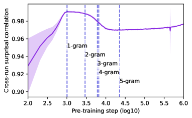
Figure 2: Mean pairwise correlation between model surprisals for different pre-training runs, at different pre-training steps. Shaded regions indicate five standard deviations from the mean. Vertical lines indicate the pre-training steps where model surprisals are maximally correlated with $n$-gram surprisals.

5 Characterizing Learning Curves

We then consider fine-grained analyses of learning curves for individual tokens in context. Motivated by previous work, we introduce five metrics for language model learning curves.

5.1 Within-Run Metrics

First, we compute four metrics for each learning curve within a pre-training run (§3.2): final surprisal, variability across pre-training steps, age of acquisition, and forgettability.

Final surprisal.

As in §3.2, surprisal quantifies the quality of a language model’s predictions for a token in context, with lower values corresponding to better predictions (Levy, 2008). For each example, we compute the mean surprisal during the last 25% of pre-training. This is closely (and inversely) related to model confidence, which Swayamdipta et al. (2020) define as the mean probability assigned to the correct label for an example during language model fine-tuning. Using surprisal, we extend this work to model pre-training.

Variability (steps).

We then measure how much model performance for an example changes across steps within a pre-training run. Specifically, we consider variability late in pre-training, when a language model has largely converged. Longer term fluctuations in performance are captured by forgettability, defined later in this section. Motivated by Swayamdipta et al. (2020), who compute the standard deviation of model probabilities during fine-tuning, we compute the standard deviation of surprisal during the last 25% of pre-training.

Age of acquisition (AoA).

We also measure when each example is learned during pre-training. Chang and Bergen (2022b) define a token’s age of acquisition (AoA) in a language model as the log-pre-training step when the model’s surprisal reaches 50% between random chance surprisal and the minimum surprisal attained by the model. Chang and Bergen (2022b) fit a sigmoid curve to the mean surprisal curve over all occurrences of the token. Because surprisal curves for individual examples are less stable than mean curves (e.g. sometimes exhibiting both peaks and dips in surprisal; Figures 1 and 3), we instead fit a GAM curve to each surprisal curve (surprisal $\sim$ log-pre-training step). We define an example’s age of acquisition as the log-pre-training step where the fitted GAM first passes 50% between random chance surprisal and the GAM’s minimum surprisal.

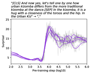
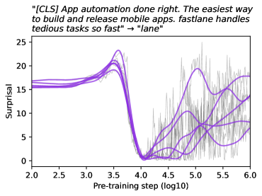
Figure 3: Learning curves for two evaluation examples from the OSCAR dataset with high forgettability scores, for the five pre-training runs. Purple lines are fitted GAM curves, one per pre-training run.

Forgettability.

Along with short-term surprisal spikes as quantified by variability (across steps), language models exhibit long-term increases in surprisal for some examples during pre-training (Xia et al., 2023). This process is described as “forgetting”. To quantify long-term surprisal increases, we measure the total surprisal increase along the GAM curve fitted to each surprisal curve. Equivalently, this is the total surprisal difference between each relative maximum and its preceding relative minimum in the curve. Larger values indicate that an example is “forgotten” to a larger extent at some point during pre-training. Example curves with high forgettability scores are shown in Figure 3.

5.2 Across-Run Metrics

Individual learning curves are similar across pre-training runs.

Each of the metrics in §5.1 correlates across pre-training runs ($r=0.652$ to $0.978$; diagonal entries in Table 2). Curves for a given example even exhibit similar peaks and dips across pre-training runs (Figure 3). Concretely, we quantify the distance between learning curves for two pre-training runs using the Euclidean distance between their fitted GAM curves. Given an example curve in one pre-training run, the curve for the same example in another pre-training run is on average (median) closer than the curve for 99.93% of other examples.

Variability (runs).

However, learning curves are not identical across runs. To quantify the cross-run variability of learning curves for a given example, we compute the mean pairwise distance (squared Euclidean distance) between the fitted GAM curves for different pre-training runs. This metric is correlated when computed using different three-run subsets of the five pre-training runs ($r=0.798$; Table 2). Our final cross-run variability metric is computed over all five pre-training runs.

	Surprisal	Var. (steps)	AoA	Forgettability_	Var. (runs)
Surprisal	0.98	0.46	0.31	0.62	0.45
Variability (steps)		0.65	0.38	0.43	0.57
AoA			0.84	0.14	0.43
Forgettability				0.79	0.51
Variability (runs)					0.80

Table 2: Pearson correlations between learning curve metrics. Diagonal entries indicate the mean correlation for that metric across pre-training runs. For variability across runs, the diagonal entry is the mean correlation between cross-run variability scores computed from different three-run subsets of the five pre-training runs.

5.3 Correlations Between Metrics

Surprisal correlates with all learning curve metrics.

Correlations between metrics are reported in Table 2. All five metrics are positively correlated with one another. High-surprisal examples exhibit more variability across pre-training steps, are learned later, are more likely to be forgotten during pre-training, and exhibit more cross-run variability. Some of these correlations are unsurprising based on our metric definitions; for example, forgettability is quantified using surprisal curve increases during pre-training, which likely lead to higher final surprisals. However, the correlation between final surprisal and forgettability is far from perfect ($r=0.622$), suggesting that some examples can be forgotten and then re-learned (high forgettability, low surprisal) or simply never learned (low forgettability, high surprisal). Upon manual inspection, we observe both of these types of curves.

Predictor	Surprisal	Var. (steps)	AoA	Forgettability	Var. (runs)
Target token log-frequency	$R^{2}=$ 0.268	$R^{2}=$ 0.248	$R^{2}=$ 0.763	$R^{2}=$ 0.083	$R^{2}=$ 0.195
+ Target 5-gram log-prob	+ 0.325	+ 0.050	(+)   + 0.001	+ 0.149	+ 0.042
+ Context log-length	+ 0.007	(+)   + 0.005	(+)   + 0.001	(+)   + 0.002	(+)   + 0.005
+ Context 1-gram log-prob	(+)   + 0.001	+ 0.006	+ 0.001	+ 0.010	+ 0.012
+ Target contextual diversity	(+)   + 0.003	(+)   + 0.000	(+)   + 0.000	(+)   + 0.001	(+)   + 0.001
+ Target part-of-speech	+ 0.009	+ 0.006	+ 0.014	+ 0.028	+ 0.026
Total variance accounted	61.2%	31.5%	78.1%	27.2%	28.1%

Table 3: Increases in adjusted $R^{2}$ values when predicting each learning curve metric, iteratively adding predictors to a linear regression. The $(+)$ symbol indicates a positive coefficient for that predictor, evaluated in three regressions (§6.1). All other coefficients are negative. Coefficients for different part-of-speech tags are described in §6.2. In the bottom row, we report the total variance accounted for in each learning curve metric using all six predictors.

6 Predicting Learning Curve Metrics

In the previous section, we defined five metrics to characterize learning curves in language models. Next, we predict each metric from specific features of each example, including $n$-gram probabilities, context likelihoods, and part-of-speech tags.

6.1 Predictors and Regressions

Each example consists of an input context and a target token (§3.2). We consider six predictors for each learning curve metric:

• Target token log-frequency: We compute the log-frequency (i.e. unigram log-probability) of the target token in the pre-training dataset.

• Target token 5-gram log-probability: To capture the likelihood of the target token based on local context, we compute the log-probability of the target token conditioned only on the previous four tokens (i.e. a 5-gram model). We compute probabilities directly from the pre-training dataset, and we use backoff to $(n-1)$-grams when an $n$-gram is not observed in the dataset (Katz, 1987). Because 5-gram log-probability is roughly linearly related to target token log-frequency ($r=0.632$), we compute the 5-gram log-probability residuals after regressing over target log-frequency. This captures the 5-gram log-probability after accounting for target token log-frequency.

• Context log-length: We compute the log of the number of context tokens.

• Context log-probability: We also compute the likelihood of the context, independent of the target token. We compute the mean log-frequency of all context tokens, equal to the negative log-perplexity of the context using a unigram language model. We use a unigram model to capture context frequency independent of word order within the context (Blei et al., 2003); longer $n$-gram models are more likely to capture probabilities of specific local constructions, even when they are distant from the target token.

• Target token contextual diversity: The diversity of contexts in which a word appears influences word learning in people, with beneficial effects in adults but potentially hindering effects in young children (Hills et al., 2010; Johns et al., 2016; Rosa et al., 2022; Chang and Bergen, 2022a). As in Hills et al. (2010), we count the number of unique tokens that appear within 30 tokens of the target token in the pre-training dataset. To remove a nonlinear effect of token frequency on this raw diversity metric, we compute the residuals after fitting a GAM curve predicting a token’s contextual diversity from its log-frequency (Chang and Bergen, 2022a). These residuals serve as a frequency-adjusted measure of a token’s contextual diversity.

• Target token part-of-speech (POS): We annotate each example with POS tags (e.g. nouns, verbs, and adjectives; §A.3) using spaCy (Honnibal et al., 2020), and we consider the POS tag of the target token. Because words can span multiple tokens, we include a feature indicating whether the target token is the first token, intermediate token, last token, or only token in a word.

We fit separate linear regressions predicting each learning curve metric from the predictors above, iteratively adding predictors in the order listed. We fit each regression to all 1M examples, predicting the mean value of each learning curve metric over all pre-training runs. We run likelihood ratio tests to assess whether each predictor is predictive of the target metric after accounting for all previous predictors, but we find that every test is highly significant ($p<0.0001$). This is likely because the large number of examples (1M) makes even small effects statistically significant. Thus, we report adjusted $R^{2}$ values that capture the magnitude of effect of each predictor, after accounting for previous predictors (Table 3).

To assess the direction of effect for each continuous predictor on each learning curve metric, we consider the coefficient for that predictor in (1) a regression containing all predictors, (2) a regression containing that predictor alone, and (3) a regression containing that predictor alone but accounting for token log-frequency in the target metric (i.e. predicting learning curve metric residuals after the log-frequency regression). In all but one case, we obtain the same direction of effect in all three regressions. Furthermore, the Pearson correlation between each pair of predictors is less than $r=0.2$, and the variance inflation factor (VIF) for each predictor is less than $1.1$. This indicates that the signs of our regression coefficients are safely interpretable. For effects of POS (a categorical variable), we consider the regression coefficient for different POS tags after accounting for all other predictors, by predicting learning curve metric residuals after regressing over the other predictors.

6.2 Results

Results are reported in Table 3, including the direction of effect for each predictor and the variance accounted for in each learning curve metric.

Target token log-frequency.

Frequent target tokens reach lower surprisals, are acquired faster, exhibit less variability within and across pre-training runs, and are less likely to be forgotten during pre-training. This is consistent with previous work showing that language models are highly reliant on token frequencies for syntactic rule learning (Wei et al., 2021), numerical reasoning (Razeghi et al., 2022), and overall word learning (Chang and Bergen, 2022b).

Target 5-gram log-probability.

Unsurprisingly, 5-gram log-probabilities correlate with lower final surprisals after accounting for target token frequency; in other words, predictions from a 5-gram model and a Transformer model are correlated beyond the effects of token frequency. More notably, higher 5-gram log-probabilities are predictive of lower learning variability both within and across pre-training runs, along with lower forgettability. The added effect of 5-gram log-probability on forgettability ($+0.149$ $R^{2}$) is even stronger than the effect of target token frequency alone ($0.083$ $R^{2}$), suggesting that conditional token probabilities play a more significant role in language model forgetting than raw token frequencies.

Less intuitively, higher 5-gram log-probabilities are correlated with marginally later ages of acquisition. We hypothesize that this is because 5-grams do take time to learn (Figure 3), but low probability 5-grams are more likely to never be learned at all, reaching their minima early in training (e.g. during the unigram learning phase). This could drive a small effect where low probability 5-grams appear to be learned earlier. Indeed, we observe qualitatively that many examples with low 5-gram probabilities and early AoAs are either never learned well (dropping only marginally below chance surprisal) or exhibit high forgettability (reaching an early minimum then increasing in surprisal). This reflects the fact that surprisal is not always an accurate measure of “learning” (§7). An early drop in surprisal does not always indicate that an example is “learned”.

Context log-length.

The remaining predictors account for far less variance in learning curve metrics than target log-frequency and 5-gram log-probability. Longer contexts correlate with lower surprisals, indicating that models successfully incorporate information from preceding context. However, longer contexts also correlate with higher variability within and across pre-training runs, higher forgettability, and later AoAs. This may be because predictions for a highly specific context are less generalizable and are thus learned less robustly by the models. This instability for long-context predictions is particularly notable as language models are increasingly used with long contexts (e.g. full conversations; OpenAI, 2022).

Context log-probability.

More frequent contexts are predictive of lower variance within and across pre-training runs, earlier acquisition, and lower forgettability. When models are repeatedly exposed to a context, regardless of the target token, their predictions stabilize earlier and with less variability. However, more frequent contexts also correlate with higher surprisals, indicating overall “worse” predictions. This may be because frequent contexts (e.g. descriptions of common situations) on average impose fewer constraints on the next token, leading to more ambiguous ground truth distributions and thus higher surprisals. If this is the case, the optimal surprisal values are simply higher in frequent contexts, but the models still learn faster and more stably given these contexts.

We note that the directions of effect for context log-probability remain stable for different window sizes of preceding context. After regressing out target token log-frequency, every coefficient sign for context log-probability remains the same for all window sizes in $\{1,2,4,...,128\}$. However, despite these consistent effects, context log-probability accounts for less than $3\%$ of the variance in each learning curve metric in all cases, even before accounting for other predictors. Frequent contexts consistently correlate with faster and more stable learning, but with only small effects.

Target contextual diversity.

Effects of contextual diversity are extremely small but statistically significant (§6.1). Tokens that appear in diverse contexts have higher final surprisals, are learned later, have greater variability within and across pre-training runs, and are more likely to be forgotten. This aligns with findings that contextual diversity hinders word learning in young children (Chang and Bergen, 2022a), contrasting with results in older children and adults (Johns et al., 2016; Rosa et al., 2022). Diverse contexts are thought to add noise to the early word learning process, introducing an excess of possible interpretations for a word.

Target part-of-speech (POS).

After accounting for other predictors, the POS tag of the target token has a small effect on each learning curve metric. Coefficients for all POS tags are reported in §A.3. Nouns, pronouns, and punctuation symbols reach lower final surprisals than verbs, adjectives, adverbs, and interjections. However, nouns are learned slower and with more variability (within and across pre-training runs) than adjectives, adverbs, and verbs, and they are more likely to be forgotten. Similarly, punctuation symbols exhibit high variability and forgettability, although they are learned early and reach low surprisals. Despite their high surprisals, interjections are learned early and stably. These results indicate that POS tags with lower surprisals are not necessarily learned more stably. Additionally, we find that different types of function words (e.g. conjunctions, prepositions, and determiners) have inconsistent effects, but they overall tend to be learned with high variability and forgettability.

The position of a token within a word also impacts learning curve metrics. Sub-word tokens after the first token in a word have low final surprisals, but they exhibit high forgettability and cross-run variability. Single-token words are the least likely to be forgotten and have the lowest cross-run variability. Compared to the POS tag of a word, a token’s position within a word has only tiny effects on within-run variability and AoA (judged by the $R^{2}$ increase from within-word position vs. POS tag itself). These results underline the importance of tokenization in language model pre-training (Rust et al., 2021); sub-word tokens are more likely to exhibit unstable learning despite low surprisals.

7 Discussion

In the previous sections, we report general patterns during language model pre-training (§4), define ways to characterize learning curves (§5), and isolate specific features that predict the speed and stability of learning for individual tokens in context (§6). Our results contribute to ongoing work studying language model pre-training dynamics, with implications for robust model deployment.

Pre-training dynamics.

We demonstrate that learning curves are more stable and converge faster for frequent tokens, $n$-gram probable tokens, and frequent contexts. These results reiterate the importance of token and $n$-gram frequencies in language model pre-training; not only is raw performance affected by frequencies (Kassner et al., 2020; Kandpal et al., 2022), pre-training instability and forgetting are significantly impacted as well. Furthermore, some parts-of-speech (e.g. nouns) and examples with longer contexts are learned more slowly and less stably. Still, our six predictors account for less than 30% of variance in some learning curve metrics (Table 3). Future work might investigate other features that influence when and how stably different examples are learned. Notably, our work only considers unseen evaluation examples; future work might identify features of the training examples that generalize to unseen examples.

Robust model deployment.

Our learning curve metrics quantify the stability of language model pre-training. Forgettability, within-run variability, and cross-run variability together contribute to the variability of a fully-trained language model’s predictions, which are notoriously erratic (Ganguli et al., 2022). Understanding which examples are likely to exhibit high variability and forgetting can inform the deployment of language models in real world applications. For example, applications might restrict language model use cases that are known to exhibit high pre-training variability or forgetting, particularly if users plan to further fine-tune the models.

Limitations and scaling.

Our work has several limitations. First, surprisal is an imperfect proxy for language model learning. A model might achieve the same surprisal at different points during pre-training by using different internal prediction strategies (e.g. predicting the same token based on frequency vs. more nuanced reasoning). Additionally, reaching some minimum surprisal does not mean that an example is “learned”; it simply indicates the best performance achieved by a model. The optimal surprisal is not necessarily zero due to the nondeterminism of language. That said, surprisal remains a common measure of language model behavior (Futrell et al., 2019; Li et al., 2021), performance (Hoffmann et al., 2022), and learning (Chang and Bergen, 2022b; Xia et al., 2023), and it requires no annotated text data to compute.

Second, we only consider language models with 124M parameters trained on 5.1B tokens. Previous work has demonstrated that learning curves differ across model sizes (Xia et al., 2023); larger models are able to “learn” some examples (usually late in pre-training) for which smaller models reach non-optimal local minima or even diverge. Larger models also exhibit less forgetting of pre-training examples (Tirumala et al., 2022), although it remains unclear whether similar mechanisms are responsible for evaluation example forgetting (i.e. surprisal increases for seen vs. unseen examples). Further research is necessary to determine the effects of model size on learning speed, variability, and forgetting. Nonetheless, previous work has documented similar behaviors for different model sizes when they achieve similar perplexities (Choshen et al., 2022; Xia et al., 2023), suggesting that pre-training dynamics in smaller models may be similar to the early dynamics of larger models.

8 Conclusion

In this work, we identify learning patterns during language model pre-training, including concrete features that predict when and how stably individual examples are acquired. We assess the impact of $n$-gram probabilities, context lengths and likelihoods, and part-of-speech tags on the speed and stability of language model learning. By identifying types of examples that are likely to be learned later and less stably, our results have implications for deploying robust language models in practice.

Appendix A Appendix

A.1 Pre-Training Details

Hyperparameter	Value
Layers	12
Embedding size	768
Hidden size	768
Intermediate hidden size	3072
Attention heads	12
Attention head size	64
Activation function	GELU
Vocab size	50004
Max sequence length	128
Position embedding	Absolute
Batch size	256
Train steps	1M
Learning rate decay	Linear
Warmup steps	10000
Learning rate	1e-4
Adam $\epsilon$	1e-6
Adam $\beta_{1}$	0.9
Adam $\beta_{2}$	0.999
Dropout	0.1
Attention dropout	0.1

Table 4: Language model pre-training hyperparameters (Devlin et al., 2019; Chang and Bergen, 2022b).

Language models are pre-trained using the Huggingface Transformers library (Wolf et al., 2020). Hyperparameters are reported in Table 4. Each model takes 2.1 weeks to train on four NVIDIA TITAN Xp GPUs or 2.5 weeks to train on one NVIDIA RTX A6000 GPU. Including pre-training and inference (evaluation surprisals), our experiments take approximately 2220 hours in A6000 GPU hours. Computing fitted GAM curves, distances between curves, $n$-gram probabilities, contextual diversities, and POS tags takes approximately 2990 CPU core hours.

A.2 Checkpoint Strategy

Assume that the steps per checkpoint $s(t)$ increases linearly as a function of the current step $t$. Assume we start with some $s(0)=s_{0}$ and end with $s(t_{1})=s_{1}$ steps per checkpoint. Then:

$$s(t)=s_{0}+\frac{s_{1}-s_{0}}{t_{1}}t$$

The rate of checkpoints per step is the inverse of steps per checkpoint, or $1/s(t)$. Excluding the checkpoint at step zero (i.e. $\text{checkpoints}(0)=0$), the number of checkpoints at step $t$ is:

$$\text{checkpoints}(t) =\text{checkpoints}(0)+\int_{0}^{t}\frac{1}{s(t)}dt$$

$$=\int_{0}^{t}\frac{t_{1}}{s_{0}t_{1}+(s_{1}-s_{0})t}dt$$

$$=\frac{t_{1}}{s_{1}-s_{0}}\text{ln}\left(1+\frac{s_{1}-s_{0}}{s_{0}t_{1}}t\right)$$

By solving for $t$, we can compute the time steps where the number of checkpoints is equal to $n=0,1,2,3,\text{etc}$. Formally, we can compute the time step $t$ for the $n^{\text{th}}$ checkpoint:

$$n =\text{checkpoints}(t)$$

$$n =\frac{t_{1}}{s_{1}-s_{0}}\text{ln}\left(1+\frac{s_{1}-s_{0}}{s_{0}t_{1}}t\right)$$

$$t =\frac{s_{0}t_{1}}{s_{1}-s_{0}}\left(\bm{e}^{n\left(\frac{s_{1}-s_{0}}{t_{1}}\right)}-1\right)$$

Note that $t$ increases exponentially as a function of the checkpoint number $n$. For our experiments, we start with $s_{0}=s(0)=100$ steps per checkpoint. We end with $s_{1}=s(1000000)=25000$ steps per checkpoint at step 1M. Then, the time step $t$ for the $n^{\text{th}}$ checkpoint is:

$$\text{step}(n) =\frac{100*1000000}{24900}\left(\bm{e}^{n\left(\frac{24900}{1000000}\right)}-1\right)$$

We round each $\text{step}(n)$ to the nearest integer, and we save model checkpoints at the selected steps until reaching 1M steps. Concretely, we save checkpoints at steps: $\text{step}(1)=101$, $\text{step}(2)=205$, …, $\text{step}(221)=981536$. We also save one checkpoint at step zero. In total, we save 222 checkpoints per pre-training run.

Surprisal
Tag	Coef.
PART	-1.28
AUX	-1.19
NOUN	-1.17
PUNCT	-1.16
PRON	-1.13
X	-1.12
SYM	-0.89
PROPN	-0.81
ADP	-0.75
VERB	-0.64
NUM	-0.60
SCONJ	-0.53
CCONJ	-0.49
INTJ	-0.47
DET	-0.41
ADJ	-0.35
ADV	-0.11
L	-0.56
I	-0.26
U	0.00
B	0.82

Var. (steps)
Tag	Coef.
INTJ	-0.03
PART	-0.02
X	-0.01
AUX	-0.01
SCONJ	-0.01
NUM	-0.01
VERB	0.00
PRON	0.00
ADV	0.00
DET	0.00
PROPN	0.00
PUNCT	0.00
ADJ	0.00
ADP	0.00
CCONJ	0.01
SYM	0.01
NOUN	0.01
B	-0.01
L	0.00
U	0.00
I	0.02

AoA
Tag	Coef.
INTJ	-0.30
PUNCT	-0.25
DET	-0.23
NUM	-0.19
X	-0.18
VERB	-0.17
ADJ	-0.17
ADV	-0.15
SYM	-0.15
PROPN	-0.13
PART	-0.12
CCONJ	-0.11
SCONJ	-0.09
NOUN	-0.07
PRON	-0.06
AUX	-0.04
ADP	0.01
U	0.00
I	0.00
L	0.03
B	0.03

Forgettability
Tag	Coef.
INTJ	-0.36
SCONJ	-0.25
ADV	-0.22
VERB	-0.19
NUM	-0.12
PART	-0.11
X	-0.09
ADJ	-0.08
PRON	-0.03
AUX	-0.01
ADP	0.05
NOUN	0.09
CCONJ	0.14
PUNCT	0.22
PROPN	0.27
SYM	0.29
DET	0.50
U	0.00
B	0.43
L	0.47
I	0.67

Var. (runs)
Tag	Coef.
INTJ	-0.23
NUM	-0.15
VERB	-0.08
ADV	-0.05
SCONJ	-0.05
AUX	-0.02
ADJ	-0.02
PART	0.02
PRON	0.03
SYM	0.04
DET	0.07
X	0.07
CCONJ	0.08
PUNCT	0.11
ADP	0.12
NOUN	0.15
PROPN	0.15
U	0.00
B	0.11
L	0.30
I	0.41

Table 5: Part-of-speech (POS) tag coefficients when predicting each learning curve metric, after accounting for other predictors (§6.1). POS tags use the Universal POS tags (Nivre et al., 2020), and we include a feature indicating whether a token is the first token (B), intermediate token (I), last token (L), or only token (U) in a word.

A.3 Part-of-Speech (POS) Coefficients

In Table 5, we report coefficients for all POS tags when predicting each learning curve metric, after accounting for other predictors (§6.1).

References

- Abadji et al. (2021) Julien Abadji, Pedro Javier Ortiz Suárez, Laurent Romary, and Benoît Sagot. 2021. Ungoliant: An optimized pipeline for the generation of a very large-scale multilingual web corpus. In Proceedings of the Workshop on Challenges in the Management of Large Corpora, pages 1–9.
- Biderman et al. (2023) Stella Biderman, Hailey Schoelkopf, Quentin Gregory Anthony, Herbie Bradley, Kyle O’Brien, Eric Hallahan, Mohammad Aflah Khan, Shivanshu Purohit, USVSN Sai Prashanth, Edward Raff, et al. 2023. Pythia: A suite for analyzing large language models across training and scaling. In International Conference on Machine Learning, pages 2397–2430.
- Blei et al. (2003) David M. Blei, Andrew Y. Ng, and Michael I. Jordan. 2003. Latent Dirichlet allocation. Journal of Machine Learning Research, 3:993–1022.
- Blevins et al. (2022) Terra Blevins, Hila Gonen, and Luke Zettlemoyer. 2022. Analyzing the mono- and cross-lingual pretraining dynamics of multilingual language models. In Proceedings of the 2022 Conference on Empirical Methods in Natural Language Processing, pages 3575–3590, Abu Dhabi, United Arab Emirates. Association for Computational Linguistics.
- Chang and Bergen (2022a) Tyler A. Chang and Benjamin K. Bergen. 2022a. Does contextual diversity hinder early word acquisition? In Proceedings of the 44th Annual Conference of the Cognitive Science Society.
- Chang and Bergen (2022b) Tyler A. Chang and Benjamin K. Bergen. 2022b. Word acquisition in neural language models. Transactions of the Association for Computational Linguistics, 10:1–16.
- Chiang et al. (2020) Cheng-Han Chiang, Sung-Feng Huang, and Hung-yi Lee. 2020. Pretrained language model embryology: The birth of ALBERT. In Proceedings of the 2020 Conference on Empirical Methods in Natural Language Processing (EMNLP), pages 6813–6828, Online. Association for Computational Linguistics.
- Choshen et al. (2022) Leshem Choshen, Guy Hacohen, Daphna Weinshall, and Omri Abend. 2022. The grammar-learning trajectories of neural language models. In Proceedings of the 60th Annual Meeting of the Association for Computational Linguistics (Volume 1: Long Papers), pages 8281–8297, Dublin, Ireland. Association for Computational Linguistics.
- Devlin et al. (2019) Jacob Devlin, Ming-Wei Chang, Kenton Lee, and Kristina Toutanova. 2019. BERT: Pre-training of deep bidirectional transformers for language understanding. In Proceedings of the 2019 Conference of the North American Chapter of the Association for Computational Linguistics: Human Language Technologies, Volume 1 (Long and Short Papers), pages 4171–4186, Minneapolis, Minnesota. Association for Computational Linguistics.
- Evanson et al. (2023) Linnea Evanson, Yair Lakretz, and Jean Rémi King. 2023. Language acquisition: Do children and language models follow similar learning stages? In Findings of the Association for Computational Linguistics: ACL 2023, pages 12205–12218, Toronto, Canada. Association for Computational Linguistics.
- Futrell et al. (2019) Richard Futrell, Ethan Wilcox, Takashi Morita, Peng Qian, Miguel Ballesteros, and Roger Levy. 2019. Neural language models as psycholinguistic subjects: Representations of syntactic state. In Proceedings of the 2019 Conference of the North American Chapter of the Association for Computational Linguistics: Human Language Technologies, Volume 1 (Long and Short Papers), pages 32–42, Minneapolis, Minnesota. Association for Computational Linguistics.
- Ganguli et al. (2022) Deep Ganguli, Danny Hernandez, Liane Lovitt, Amanda Askell, Yuntao Bai, Anna Chen, Tom Conerly, Nova Dassarma, Dawn Drain, Nelson Elhage, Sheer El Showk, Stanislav Fort, Zac Hatfield-Dodds, Tom Henighan, Scott Johnston, Andy Jones, Nicholas Joseph, Jackson Kernian, Shauna Kravec, Ben Mann, Neel Nanda, Kamal Ndousse, Catherine Olsson, Daniela Amodei, Tom Brown, Jared Kaplan, Sam McCandlish, Christopher Olah, Dario Amodei, and Jack Clark. 2022. Predictability and surprise in large generative models. In Proceedings of the ACM Conference on Fairness, Accountability, and Transparency, page 1747–1764, New York, NY, USA. Association for Computing Machinery.
- Google (2023) Google. 2023. PaLM 2 technical report. arXiv.
- Hills et al. (2010) Thomas Hills, Josita Maouene, Brian Riordan, and Linda Smith. 2010. The associative structure of language: Contextual diversity in early word learning. Journal of Memory and Language, 63(3):259–273.
- Hoffmann et al. (2022) Jordan Hoffmann, Sebastian Borgeaud, Arthur Mensch, Elena Buchatskaya, Trevor Cai, Eliza Rutherford, Diego de las Casas, Lisa Anne Hendricks, Johannes Welbl, Aidan Clark, Tom Hennigan, Eric Noland, Katherine Millican, George van den Driessche, Bogdan Damoc, Aurelia Guy, Simon Osindero, Karen Simonyan, Erich Elsen, Oriol Vinyals, Jack William Rae, and Laurent Sifre. 2022. Training compute-optimal large language models. In Advances in Neural Information Processing Systems.
- Holtzman et al. (2020) Ari Holtzman, Jan Buys, Li Du, Maxwell Forbes, and Yejin Choi. 2020. The curious case of neural text degeneration. In International Conference on Learning Representations.
- Honnibal et al. (2020) Matthew Honnibal, Ines Montani, Sofie Van Landeghem, and Adriane Boyd. 2020. spaCy: Industrial-strength natural language processing in python. SpaCy.
- Johns et al. (2016) Brendan Johns, Melody Dye, and Michael Jones. 2016. The influence of contextual diversity on word learning. Psychonomic Bulletin and Review, 23:1214–1220.
- Kandpal et al. (2022) Nikhil Kandpal, Haikang Deng, Adam Roberts, Eric Wallace, and Colin Raffel. 2022. Large language models struggle to learn long-tail knowledge. In Inernational Conference on Machine Learning.
- Kassner et al. (2020) Nora Kassner, Benno Krojer, and Hinrich Schütze. 2020. Are pretrained language models symbolic reasoners over knowledge? In Proceedings of the 24th Conference on Computational Natural Language Learning, pages 552–564, Online. Association for Computational Linguistics.
- Katz (1987) Slava Katz. 1987. Estimation of probabilities from sparse data for the language model component of a speech recognizer. IEEE Transactions on Acoustics, Speech, and Signal Processing, 35(3):400–401.
- Levy (2008) Roger Levy. 2008. Expectation-based syntactic comprehension. Cognition, 106(3):1126–1177.
- Li et al. (2021) Bai Li, Zining Zhu, Guillaume Thomas, Yang Xu, and Frank Rudzicz. 2021. How is BERT surprised? layerwise detection of linguistic anomalies. In Proceedings of the 59th Annual Meeting of the Association for Computational Linguistics and the 11th International Joint Conference on Natural Language Processing (Volume 1: Long Papers), pages 4215–4228, Online. Association for Computational Linguistics.
- Liu et al. (2021) Zeyu Liu, Yizhong Wang, Jungo Kasai, Hannaneh Hajishirzi, and Noah A. Smith. 2021. Probing across time: What does RoBERTa know and when? In Findings of the Association for Computational Linguistics: EMNLP 2021, pages 820–842, Punta Cana, Dominican Republic. Association for Computational Linguistics.
- Mahowald et al. (2023) Kyle Mahowald, Anna A. Ivanova, Idan A. Blank, Nancy Kanwisher, Joshua B. Tenenbaum, and Evelina Fedorenko. 2023. Dissociating language and thought in large language models: A cognitive perspective. arXiv.
- Nivre et al. (2020) Joakim Nivre, Marie-Catherine de Marneffe, Filip Ginter, Jan Hajič, Christopher D. Manning, Sampo Pyysalo, Sebastian Schuster, Francis Tyers, and Daniel Zeman. 2020. Universal Dependencies v2: An evergrowing multilingual treebank collection. In Proceedings of the Twelfth Language Resources and Evaluation Conference, pages 4034–4043, Marseille, France. European Language Resources Association.
- Olsson et al. (2022) Catherine Olsson, Nelson Elhage, Neel Nanda, Nicholas Joseph, Nova DasSarma, Tom Henighan, Benjamin Mann, Amanda Askell, Yuntao Bai, Anna Chen, Tom Conerly, Dawn Drain, Deep Ganguli, Zac Hatfield-Dodds, Danny Hernandez, Scott Johnston, Andy Jones, John Kernion, Liane Lovitt, Kamal Ndousse, Dario Amodei, Tom B. Brown, Jack Clark, Jared Kaplan, Sam McCandlish, and Chris Olah. 2022. In-context learning and induction heads. arXiv.
- OpenAI (2022) OpenAI. 2022. ChatGPT: Optimizing language models for dialogue. OpenAI Blog.
- Radford et al. (2018) Alec Radford, Karthik Narasimhan, Tim Salimans, and Ilya Sutskever. 2018. Improving language understanding by generative pre-training. OpenAI.
- Radford et al. (2019) Alec Radford, Jeff Wu, Rewon Child, David Luan, Dario Amodei, and Ilya Sutskever. 2019. Language models are unsupervised multitask learners. OpenAI Technical Report.
- Razeghi et al. (2022) Yasaman Razeghi, Robert L Logan IV, Matt Gardner, and Sameer Singh. 2022. Impact of pretraining term frequencies on few-shot numerical reasoning. In Findings of the Association for Computational Linguistics: EMNLP 2022, pages 840–854, Abu Dhabi, United Arab Emirates. Association for Computational Linguistics.
- Rosa et al. (2022) Eva Rosa, Rafael Salom, and Manuel Perea. 2022. Contextual diversity favors the learning of new words in children regardless of their comprehension skills. Journal of Experimental Child Psychology, 214.
- Rust et al. (2021) Phillip Rust, Jonas Pfeiffer, Ivan Vulić, Sebastian Ruder, and Iryna Gurevych. 2021. How good is your tokenizer? on the monolingual performance of multilingual language models. In Proceedings of the 59th Annual Meeting of the Association for Computational Linguistics and the 11th International Joint Conference on Natural Language Processing (Volume 1: Long Papers), pages 3118–3135, Online. Association for Computational Linguistics.
- Saphra and Lopez (2019) Naomi Saphra and Adam Lopez. 2019. Understanding learning dynamics of language models with SVCCA. In Proceedings of the 2019 Conference of the North American Chapter of the Association for Computational Linguistics: Human Language Technologies, Volume 1 (Long and Short Papers), pages 3257–3267, Minneapolis, Minnesota. Association for Computational Linguistics.
- Sellam et al. (2022) Thibault Sellam, Steve Yadlowsky, Jason Wei, Naomi Saphra, Alexander D’Amour, Tal Linzen, Jasmijn Bastings, Iulia Turc, Jacob Eisenstein, Dipanjan Das, et al. 2022. The MultiBERTs: BERT reproductions for robustness analysis. International Conference on Learning Representations.
- Swayamdipta et al. (2020) Swabha Swayamdipta, Roy Schwartz, Nicholas Lourie, Yizhong Wang, Hannaneh Hajishirzi, Noah A. Smith, and Yejin Choi. 2020. Dataset cartography: Mapping and diagnosing datasets with training dynamics. In Proceedings of the 2020 Conference on Empirical Methods in Natural Language Processing (EMNLP), pages 9275–9293, Online. Association for Computational Linguistics.
- Tirumala et al. (2022) Kushal Tirumala, Aram H. Markosyan, Luke Zettlemoyer, and Armen Aghajanyan. 2022. Memorization without overfitting: Analyzing the training dynamics of large language models. In Advances in Neural Information Processing Systems.
- Warstadt and Bowman (2023) Alex Warstadt and Samuel R. Bowman. 2023. What Artificial Neural Networks Can Tell Us About Human Language Acquisition, chapter Algebraic Structures in Natural Language. Taylor & Francis.
- Wei et al. (2021) Jason Wei, Dan Garrette, Tal Linzen, and Ellie Pavlick. 2021. Frequency effects on syntactic rule learning in transformers. In Proceedings of the 2021 Conference on Empirical Methods in Natural Language Processing, pages 932–948, Online and Punta Cana, Dominican Republic. Association for Computational Linguistics.
- Wolf et al. (2020) Thomas Wolf, Lysandre Debut, Victor Sanh, Julien Chaumond, Clement Delangue, Anthony Moi, Pierric Cistac, Tim Rault, Remi Louf, Morgan Funtowicz, Joe Davison, Sam Shleifer, Patrick von Platen, Clara Ma, Yacine Jernite, Julien Plu, Canwen Xu, Teven Le Scao, Sylvain Gugger, Mariama Drame, Quentin Lhoest, and Alexander Rush. 2020. Transformers: State-of-the-art natural language processing. In Proceedings of the 2020 Conference on Empirical Methods in Natural Language Processing: System Demonstrations, pages 38–45, Online. Association for Computational Linguistics.
- Xia et al. (2023) Mengzhou Xia, Mikel Artetxe, Chunting Zhou, Xi Victoria Lin, Ramakanth Pasunuru, Danqi Chen, Luke Zettlemoyer, and Veselin Stoyanov. 2023. Training trajectories of language models across scales. In Proceedings of the 61st Annual Meeting of the Association for Computational Linguistics (Volume 1: Long Papers), pages 13711–13738, Toronto, Canada. Association for Computational Linguistics.