A coupled high-accuracy phase-field fluid-structure interaction framework for Stokes fluid-filled fracture surrounded by an elastic medium

Abstract

In this work, we couple a high-accuracy phase-field fracture reconstruction approach iteratively to fluid-structure interaction. The key motivation is to utilize phase-field modelling to compute the fracture path. A mesh reconstruction allows a switch from interface-capturing to interface-tracking in which the coupling conditions can be realized in a highly accurate fashion. Consequently, inside the fracture, a Stokes flow can be modelled that is coupled to the surrounding elastic medium. A fully coupled approach is obtained by iterating between the phase-field and the fluid-structure interaction model. The resulting algorithm is demonstrated for several numerical examples of quasi-static brittle fractures. We consider both stationary and quasi-stationary problems. In the latter, the dynamics arise through an incrementally increasing given pressure.

[1] organization=University of Vienna, Faculty for Mathematics, addressline=Oskar-Morgenstern-Platz 1, city=Vienna, postcode=1090, country=Austria

[2] organization=Friedrich Schiller University Jena, Institute for Mathematics, addressline=Ernst-Abbe-Platz 2, city=Jena, postcode=07743, country=Germany

[3] organization=Leibniz University Hannover, Institute for Applied Mathematics, addressline=Welfengarten 1, city=Hannover, postcode=30167, country=Germany

1 Introduction

The starting point of the current work is a novel high-accuracy phase-field fracture framework with interface reconstructions [1]. The closest related works with similar motivations are [2, 3, 4], in which both the phase-field and level set/extended finite element (XFEM) approaches are coupled. Next, [5] also has the same motivation as we do in which a k-nearest neighbor method is used to compute the normal directions of the crack, and a subsequent reconstruction. Moreover, we mention [6] and [7] in which level-set formulations from the phase-field function are used to compute normal vectors or construct finite element representations of the fracture width. Improvements in terms of accuracy of the latter work, namely [7], is one specific motivation of our current work. Related studies that are also concerned with high-accuracy representations of quantities of interest in the fracture process zone are [8], where the accurate resolution of stresses in the fracture area was achieved by employing combined discretization schemes of finite element and finite volume types, and [9], where the phase-field formulation was enhanced with an additional external driving force.

Various groups have studied fractional phase-field modelling from which the fracture path is computed [10, 11, 12, 13, 14, 15, 16, 17, 18]. Monographs and extended papers of phase-field methods for fracture propagation are [19, 15, 20, 21, 22, 23]. On the other hand, fluid-structure interaction (FSI) in arbitrary Lagrangian-Eulerian coordinates (ALE) was proposed in [24, 25]; see also the overview [26]. Some theoretical work on ALE schemes was done in [27, 28]. Books and monographs on fluid-structure interaction include [29, 30, 31, 32, 33, 34, 35]. The combination of phase fields with fluid-structure interaction was subject in [36, 37, 38] and [21, Chapter 11.8].

As previously outlined, we begin with our prior work [1], in which we used the fracture phase-field to determine the fracture path and reconstruct the open fluid-filled crack geometry to have a sharp interface between the fracture sub-domain and the surrounding medium. This idea is relevant in applications where both a flexible method for largely moving or growing interfaces is required, and high accuracy of interface conditions is necessary due to different interacting physics phenomena. One first application can be found in subsurface modelling, for instance, porous media applications with interfaces [39, 40, 41, 42, 43, 44, 45, 46, 47, 48, 49, 50, 22, 51, 52, 53], non-isothermal phase-field fracture [54, 55, 56, 57], or computational medicine with fluid-structure interaction [58, 35, 33, 59, 60, 61] in which interfaces must be resolved with high accuracy in order to keep discretization errors in the coupling conditions sufficiently small.

The current work’s main objective is to extend the one-way coupling proposed in [1] to a fully coupled algorithm. However, this includes several modifications on both the mathematical and numerical levels. Conceptionally, the high-accuracy interface reconstruction framework from [1] is employed in which the fracture path is computed with a phase field. Then, the crack opening displacements are computed to construct the new fluid-filled fracture domain. This allows the application of an interface-tracking approach with an accurate partition into solid and fluid subdomains. In each domain, in principle, any required physics can be posed. For simplicity, we focus on elastic solids and linear incompressible (Stokes) flow. The overall phase-field fracture fluid-structure interaction is decoupled and solved iteratively while each sub-problem remains non-linear. The phase-field problem consists of displacements and the phase-field function that are treated in a fully coupled fashion, where the phase-field function is subject to a crack irreversibility condition. These two properties result in a non-linear phase-field problem. The fluid-structure interaction problem is non-linear due to the ALE approach despite working with a linear Stokes flow. In both situations, Newton-type solvers are employed. As the reconstruction procedure allows for interface-tracking methods, the interface conditions can be prescribed and realized directly on the interface. This is usually difficult in phase-field methods as it is an interface-capturing approach.

The starting point for our phase-field model is [62, Section 2], in which a porous media mechanics step is proposed using kinematic (continuity of principal variables) and dynamic (continuity of fluxes) interface conditions between the fracture and the porous medium. In [62, p. 7], Gauss’ divergence theorem was employed to rewrite the sharp interface conditions as domain integrals to account for the property in phase-field methods that the interface is given in a smeared fashion rather than a precise manifold. This type of approach has been applied in most of the references mentioned previously on porous media applications with interfaces.

To the best of our knowledge, applying the sharp interface conditions directly in the phase-field problem, rather than the domain integrals resulting from applying Gauss’ divergence theorem, was never utilized in the published literature. Our motivation for this approach is as follows. The original formulation, i.e., [63, 10], starts from a sharp fracture, which is then approximated for numerical purposes via elliptic Ambrosio-Tortorelli functionals [64, 65]. In this work, go back to sharp interface approximations. Here, we note that some studies consider fractures and their flow on dimensionally-reduced objects, e.g., [66, 67], which are, however, given (and fixed) in advance. In order to develop concepts that can utilize one of the main intriguing capabilities of phase-field, namely growing, curvilinear fractures, merging and branching with relative ease, we aim to utilize phase-field as a state-of-the-art ‘crack-growth’ module. In order to have all capabilities at hand on the physics in the fracture from first principle physics laws, e.g., using Stokes or Navier-Stokes, starting with a dimensionally-reduced fracture model is not an option for us. Our overall aim is to have the fracture domain and the surrounding medium in the same dimension. Here, most current works (see the many previous references on phase-field fracture) employ the physics directly in the phase-field approach, resulting in multiphysics phase-field fracture. However, the accurate description of interface conditions is always a point of concern, in addition to relative coarse sub-meshes in the fracture zone, giving rough finite element approximations only. Our main motivation is to overcome these last two limitations by our proposed mesh reconstruction to prescribe interface conditions on a sharp interface resolved with an interface-tracking method and, second, to have the flexibility to have fine meshes with sufficiently small finite element discretization errors. We notice that fluid-structure interaction with an elastic surrounding medium and Stokes flow in the fracture is simply a prototype example, and any other physics, e.g., heat transfer, towards thermo-hydraulic-mechanical fracture, or more complicated fracture flow models, e.g., Navier-Stokes or non-Newtonian flow, can be utilized following the same descriptions.

Our first objective is a mathematical formulation of such a pressurized phase-field fracture problem statement. This formulation of the phase-field problem is then used to couple with the ALE fluid-structure interaction problem via our mesh reconstruction approach and the FSI pressure. The second objective is the design of a fully coupled algorithm in which we iterate between pressurized phase-field fracture and fluid-structure interaction that increases the accuracy not only to prescribe the interface conditions themselves but also to enhance the accuracy of the overall coupled problem to a given tolerance.

As the prescribed pressure drives the phase field, we will couple the phase-field problem to the fluid-structure interaction solution through the FSI pressure. However, the FSI pressure only exists in the reconstructed wide-open fluid domain rather than the entire domain. Furthermore, the sharp phase-field crack is a slim domain. Consequently, we need to use an averaged fluid-structure interaction pressure in the phase-field formulation.

The final algorithm then consist of the computation of the phase-field problem, the reconstruction of the fluid-filled open crack domain, the computation of the fluid-structure interaction problem and then the back coupling of an averaged FSI pressure to the phase-field problem. This final algorithm is demonstrated for some prototypical scenarios, which include both stationary and propagating fractures. In summary, the novelties are:

• Pressurized phase-field fracture problem statement with fracture interface terms;

• Design of a fully coupled algorithm for phase-field fluid-structure interaction;

• Quasi-static time-dependence with propagating fractures.

The outline of this paper is as follows. In Section 2, we present our phase-field fluid-structure interaction approach. Next, in Section 3, we discuss the discretization of the phase-field and FSI problems, the fluid-filled crack interface reconstruction, the pressure coupling and the numerical solution of the discrete problem. This then guides us to the design of a final algorithm. In Section 4, several numerical tests substantiate our proposed approach. Finally, our work is summarised in Section 5.

2 A phase-field fluid-structure interaction framework

In this section, we formulate our high-accuracy phase-field fracture fluid-structure interaction framework [1]. In this framework, the fracture shape is determined by a phase-field method. In Section 2.2, our phase-field fracture model starts from the original work [10] in which sharp interfaces are approximated for numerical purposes via elliptic Ambrosio-Tortorelli functionals [64, 65]. Additional physics, e.g., pressure inside the fracture, can be included via two ways, namely Gauss’ divergence theorem [62, 68] or keeping explicitly the interface integral. The latter is newly investigated in this work as it was so far in phase-field fracture due to the smeared zone not being of interest. We notice that Gauss’ divergence theorem is not limited to pressure; for instance, temperatures [21, Chapter 11] can be described similarly. The crack irreversibility constraint is relaxed using a penalization approach. We use the phase-field solution to reconstruct the cracked domain, which fully resolves the interface between the fluid-filled crack and the intact solid domain. Using this partition, we solve a creeping flow problem inside the crack coupled to the fluid’s elastic medium. In particular, we derive this fluid-structure interaction problem in Section 2.3 by assuming the surrounding medium as an elastic solid, and the flow in the fracture of Stokes type.

2.1 Notation

In the following, let $\Omega\subset\mathbb{R}^{d}$, $d\in\{2,3\}$, be the total domain under consideration. Then let $\mathscr{C}\subset\Omega$ denote the fracture in our domain and $\pazocal{S}\subset\Omega$ denote the intact domain. In a phase-field approach, the fracture $\mathscr{C}$ is approximated by $\pazocal{C}\subset\mathbb{R}^{d}$ with the help of an elliptic (Ambrosio-Tortorelli) functional [64, 65]. For fracture formulations posed in a variational setting, this was first proposed in [10]. The inner fracture boundary is denoted by $\partial\pazocal{C}$. We emphasise that the domains $\pazocal{S},\pazocal{C}$, and the boundary $\partial\pazocal{C}$ depend on the choice of the so-called phase-field regularisation parameter $\varepsilon>0$. Details of this parameter are presented below. Finally, we denote the $L^{2}(\Omega)$ scalar product with $(\cdot,\cdot)$.

2.2 Phase-Field Fracture

We introduce the equations governing the phase-field fracture model used in this work to model the fluid-filled crack. As we build on our earlier work [1], this is, in most parts, a repetition of [1, Section 2.2], which we provide for completeness. However, the phase-field model with sharp interface conditions 3 is novel in comparison to [1] and the literature.

The weak formulations for our phase-field fracture model are given in an incremental (i.e., time-discretised) formulation. This is based on a pressurised fracture extension of a quasi-static variational fracture model [63, 10] as presented in [62, 68]. We first state a classical formulation and then present the linearised and regularised formulation we later use in our implementation.

The fracture problem requires two unknowns: the vector-valued displacement field $\bm{u}$ and the scalar-valued phase-field function $\varphi$. The phase-field function indicates the presence of a crack by taking the value $\varphi=1$ in the intact domain $\pazocal{S}$, the value $\varphi=0$ inside the crack $\pazocal{C}$ and a smooth transition between the two in a region of width $\varepsilon>0$ around the interface between the open crack and the intact domain, denoted now by $\pazocal{S}$ and $\pazocal{C}$. In the context of a fluid-filled crack, these domains will later be denoted as $\pazocal{S}$ and $\pazocal{F}$, respectively. Since an open crack cannot reseal, the phase field is subject to the crack irreversibility constraint $\partial_{t}\varphi\leq 0$. For the purpose of our phase-field model, the continuous irreversibility constraint is approximated through a difference quotient by

$$\varphi\leq\varphi^{old}.$$

Later, $\varphi^{old}$ will denote the solution at the previous iteration step $\varphi^{m-1}$, and the current solution $\varphi\coloneqq\varphi^{m}$.

For simplicity, we will assume homogeneous Dirichlet conditions on the outer boundary $\partial\Omega$ for the displacement field. Therefore, we consider the function spaces $W\coloneqq H^{1}(\Omega)$, $\bm{V}\coloneqq[H^{1}_{0}(\Omega)]^{d}$ and the convex set

$$K\coloneqq\{w\in H^{1}(\Omega)|\,w\leq\varphi^{old}\leq 1\text{ a.e. on }\Omega\}.$$

The latter two are the the solution sets, respectively. An important object in our work is the interface $\partial\pazocal{C}$ with the conditions (for pressurized fractures):

$$p_{\pazocal{S}} =p_{\pazocal{F}},$$

$$\sigma_{\pazocal{S}}\bm{n} =\sigma_{\pazocal{F}}\bm{n},$$

where the normal vector $\bm{n}$ points into the crack region. As the interface is usually only known as a smeared region in phase-field fracture, in the original work [62] (see also [21, 11.4.1.2]) Gauss’ divergence theorem was employed yielding for the second condition

$$\int_{\partial\pazocal{C}}\sigma_{\pazocal{S}}\bm{n}\,ds =\int_{\partial\pazocal{C}}\sigma_{\pazocal{F}}\bm{n}\,ds$$ (1)

$$=\int_{\partial\pazocal{C}}p\bm{n}\cdot\bm{u}\,ds$$ (2)

$$=\int_{\pazocal{F}}\nabla\cdot(p\bm{u})\,dx-\int_{\partial\Omega}p\bm{n}\cdot\bm{u}\,ds$$ (3)

$$=\int_{\pazocal{F}}(\bm{u}\nabla p+p\nabla\cdot\bm{u})\,dx-\int_{\partial\Omega}p\bm{n}\cdot\bm{u}\,ds$$ (4)

$$=\int_{\pazocal{F}}(\bm{u}\nabla p+p\nabla\cdot\bm{u})\,dx.$$ (5)

In (2) of this equation chain, we assumed that the leading order of the stress $\sigma_{\pazocal{F}}=-pI+\rho\nu(\nabla v+\nabla v^{T})$ is the pressure, resulting in $\sigma_{\pazocal{F}}\approx-pI$. In (3), Gauss’ divergence theorem is applied. In (5), homogeneous Dirichlet conditions on $\bm{u}=0$ on $\partial\Omega$ are assumed. Despite the fact that the sharp interface representation is the starting point, in the following we first recapitulate the pressurized phase-field fracture model based on (5), i.e., 1 and 2, as these present our standard model so far. Then, in 3 the model employing (2) is considered.

To this end, the phase-field fracture model is given by a coupled variational inequality system (CVIS) [21] and reads as follows.

Formulation 1.

Let the pressure $p\in W^{1,\infty}(\Omega)$, Dirichlet boundary data $\bm{u}_{D}$ on $\partial\Omega$, and the initial condition $\varphi(0)\coloneqq\varphi_{0}$ be given. For the iteration steps $m=1,2,3,\dots,M$, we compute the following problem: Find $(\bm{u},\varphi)\coloneqq(\bm{u}^{m},\varphi^{m})\in\{\bm{u}_{D}+\bm{V}\}\times K$, such that

$$\Bigl{(}g(\varphi)\;\bm{\sigma}_{s}(\bm{u}),\bm{e}({\bm{w}})\Bigr{)}+({\varphi}^{2}p,\nabla\cdot{\bm{w}})+({\varphi}^{2}\nabla p,\bm{w}) =0\quad\forall\bm{w}\in\bm{V},$$ (6a)

$$\begin{multlined}(1-\kappa)({\varphi}\;\bm{\sigma}_{s}(\bm{u})\mathrel{\mathop{\mathchar 58\relax}}\bm{e}(\bm{u}),\psi{-\varphi})+2({\varphi}\;p\;\nabla\cdot\bm{u},\psi{-\varphi})+2({\varphi}\;\nabla p\;\bm{u},\psi)\\ +G_{c}\Bigl{(}-\frac{1}{\varepsilon}(1-\varphi,\psi{-\varphi})+\varepsilon(\nabla\varphi,\nabla(\psi-{\varphi}))\Bigr{)}\end{multlined}(1-\kappa)({\varphi}\;\bm{\sigma}_{s}(\bm{u})\mathrel{\mathop{\mathchar 58\relax}}\bm{e}(\bm{u}),\psi{-\varphi})+2({\varphi}\;p\;\nabla\cdot\bm{u},\psi{-\varphi})+2({\varphi}\;\nabla p\;\bm{u},\psi)\\ +G_{c}\Bigl{(}-\frac{1}{\varepsilon}(1-\varphi,\psi{-\varphi})+\varepsilon(\nabla\varphi,\nabla(\psi-{\varphi}))\Bigr{)} \geq 0\quad\forall\psi\in K\cap L^{\infty}(\Omega).$$ (6d)

Therein, we have the degradation function

$$g(\varphi)\coloneqq(1-\kappa){\varphi}^{2}+\kappa,$$

with the bulk regularisation parameter $\kappa>0$, the phase-field regularisation parameter $\varepsilon>0$, the Cauchy stress tensor

$$\bm{\sigma}_{s}=2\mu\bm{e}(\bm{u})+\lambda tr(\bm{e}(\bm{u}))I,$$

with the Lamé parameters $\mu,\lambda>0$, the identity matrix $I\in\mathbb{R}^{2\times 2}$ and the linearised strain tensor

$$\bm{e}(\bm{u})=\frac{1}{2}(\nabla\bm{u}+\nabla\bm{u}^{T}).$$

First, we note that the phase-field regularization parameter $\varepsilon$ is linked to the bulk regularization $\kappa$ and the local mesh size parameter $h$; see [69] for a numerical analysis in terms of image segmentation, where the main regularization functional (Ambrosio-Tortorelli type [64, 65]) is similar to phase-field fracture, as well as [10, Section 2.1.2] and [21, Section 5.5]. On the other hand, $\varepsilon$ is known as a length scale in engineering and can be interpreted as a fixed number representing micro-cracks around the fracture zone; see, e.g., [12, 70]. For typical numerical-computational convergence studies, a decision must be made about which type of convergence is to be studied. For discretization errors only, $\varepsilon$ must be fixed. If the interaction of $\varepsilon$ and $h$ towards sharp interface limits is of interest, $\varepsilon$ should also vary. However, significant computational resources, mesh adaptivity and parallel computing are needed to study asymptotic limits [71]. Furthermore, $\varepsilon$ impacts crack nucleation, e.g., [72, 73], which limits its choice. Finally, we note that as an extension, $\varepsilon$ can be made arbitrary at the cost of introducing additional parameters in the total energy-functional [17].

Next, we note that the system (6) does not explicitly contain time-derivatives. In our setting, the time $t$ enters through time-dependent, i.e., incrementally dependent since we work in a quasi-static regime, right-hand side forces, e.g., a time-dependent pressure force $p\coloneqq p(t)$. Due to the quasi-static nature of this problem formulation, we derive the time-discretised formulation with some further approximations. Our first approximation relaxes the non-linear behaviour in the first term $g(\varphi)\;\bm{\sigma}_{s}(\bm{u})$ of the displacement equation by using

$$\varphi\approx\varphi^{m-1},$$

yielding $g(\varphi^{m-1})$. This idea is based on the extrapolation introduced in [74] and is numerically justified specifically for slowly growing fractures [21, Chapter 6], while counter-examples for fast-growing fractures were found in [75].

As $\varphi^{m-1}$ introduces an approximation error of order $O(\tau_{m}-\tau_{m-1})$ for smaller steps, the error vanishes, or fully monolithic schemes (again [75]) or an additional iteration [76] must be introduced.

The second approximation is related to the inequality constraint. In this work, we relax the constraint by simple penalisation [77] (see also [21, Chapter 5]), i.e.,

$$\varphi\leq\varphi^{m-1}\quad\rightarrow\quad\gamma(\varphi-\varphi^{m-1})^{+}.$$

Here, $(x)^{+}=x$ for $x>0$ and $(x)^{+}=0$ for $x\leq 0$, and where $\gamma>0$ is a penalty parameter. We then arrive at the regularised scheme

Formulation 2.

Let $p\in W^{1,\infty}(\Omega)$ and the initial condition $\varphi(0)\coloneqq\varphi_{0}$ be given. For the iteration steps $m=1,2,3,\dots,M$, we compute: Find $(\bm{u},\varphi)\coloneqq(\bm{u}^{m},\varphi^{m})\in\bm{V}\times W$ such that

$$\Bigl{(}g(\varphi^{m-1})\;\sigma(\bm{u}),\bm{e}({\bm{w}})\Bigr{)}+({\varphi^{m-1}}^{2}p,\nabla\cdot{\bm{w}})+({\varphi^{m-1}}^{2}\nabla p,\bm{w}) =0\quad\forall\bm{w}\in\bm{V},$$ (7a)

$$\begin{multlined}(1-\kappa)({\varphi}\;\sigma(\bm{u})\mathrel{\mathop{\mathchar 58\relax}}\bm{e}(\bm{u}),\psi)+2({\varphi}\;p\;\nabla\cdot\bm{u},\psi)+2({\varphi}\;\nabla p\;\bm{u},\psi)\\ +G_{c}\Bigl{(}-\frac{1}{\varepsilon}(1-\varphi,\psi)+\varepsilon(\nabla\varphi,\nabla\psi)\Bigr{)}+(\gamma(\varphi-\varphi^{m-1})^{+},\psi)\end{multlined}(1-\kappa)({\varphi}\;\sigma(\bm{u})\mathrel{\mathop{\mathchar 58\relax}}\bm{e}(\bm{u}),\psi)+2({\varphi}\;p\;\nabla\cdot\bm{u},\psi)+2({\varphi}\;\nabla p\;\bm{u},\psi)\\ +G_{c}\Bigl{(}-\frac{1}{\varepsilon}(1-\varphi,\psi)+\varepsilon(\nabla\varphi,\nabla\psi)\Bigr{)}+(\gamma(\varphi-\varphi^{m-1})^{+},\psi) =0\quad\forall\psi\in W.$$ (7d)

Note that we assume a varying pressure $p$, which requires to use the pressure gradient $\nabla p$ [39, (2.30) and (2.31)] in extension to our previous work [1].

Remark 1.

We call the steps $\tau_{m}$ with index $m$ in this work ‘iteration’ steps, which are used to satisfy the irreversibility constraint. In previous works, they were introduced as incremental steps, pseudo-time steps, or time steps. We choose iteration steps in this work to better distinguish from (time) steps $t_{n}$ with index $n$ used to advance the overall coupled system of phase-field mesh reconstruction and fluid-structure interaction.

The previous formulation is based on an interface law is formulated as domain integral using Gauss’ divergence theorem [62, Section 2]. An equivalent formulation can be given by directly using the interface term. This then is given as follows.

Formulation 3.

Let $p\in L^{\infty}(\Omega)$ and the initial condition $\varphi(0)\coloneqq\varphi_{0}$ be given. For the iteration steps $m=1,2,3,\dots,M$, we compute: Find $(\bm{u},\varphi)\coloneqq(\bm{u}^{m},\varphi^{m})\in\bm{V}\times W$ such that

$$\Bigl{(}g(\varphi^{m-1})\;\sigma(\bm{u}),\bm{e}({\bm{w}})\Bigr{)}+\int_{\partial\pazocal{C}}{\varphi^{m-1}}^{2}p\bm{n}\cdot\bm{w}\,ds =0\quad\forall\bm{w}\in\bm{V},$$ (8a)

$$\begin{multlined}(1-\kappa)({\varphi}\;\sigma(\bm{u})\mathrel{\mathop{\mathchar 58\relax}}\bm{e}(\bm{u}),\psi)+2\int_{\partial\pazocal{C}}\varphi p\bm{n}\cdot\bm{u}\psi\,ds\\ +G_{c}\Bigl{(}-\frac{1}{\varepsilon}(1-\varphi,\psi)+\varepsilon(\nabla\varphi,\nabla\psi)\Bigr{)}+(\gamma(\varphi-\varphi^{m-1})^{+},\psi)\end{multlined}(1-\kappa)({\varphi}\;\sigma(\bm{u})\mathrel{\mathop{\mathchar 58\relax}}\bm{e}(\bm{u}),\psi)+2\int_{\partial\pazocal{C}}\varphi p\bm{n}\cdot\bm{u}\psi\,ds\\ +G_{c}\Bigl{(}-\frac{1}{\varepsilon}(1-\varphi,\psi)+\varepsilon(\nabla\varphi,\nabla\psi)\Bigr{)}+(\gamma(\varphi-\varphi^{m-1})^{+},\psi) =0\quad\forall\psi\in W.$$ (8d)

Here, the normal vector $\bm{n}$ points into the crack region.

To the best of our knowledge, 3 has not been used in the literature thus far. This can be attributed to the fact that it contradicts the concept of a phase field in the sense that a phase-field model should not require explicit knowledge of the interface position. However, in our proposed coupling with fluid-structure interaction, and with the aim to provide a high-accuracy framework, 3 is of interest. Consequently, we will use (8) as the system of equations to compute the phase-field fracture in each iteration. As we are in a quasi-stationary regime here, we compute each phase-field with a total of $M=5$ iteration steps. In each of these iteration steps, we then use Newton’s method to solve the resulting non-linear problem up to a tolerance of $10^{-8}$. Time dependence will only enter our system through time-dependent pressure and consequently changing crack domains.

In [1], we presented a number of methods to reconstruct the geometry of an open, fluid-filled crack resulting from a phase-field model. Here, we will focus on the approach where the resulting computational mesh resolves this geometry. With the mesh containing the resolved interface between the open crack and the surrounding solid at hand, we can now describe the fluid-structure interaction problem between the fluid-filled crack and the solid domain surrounding it. With our explicit interface reconstructions of the fracture surface, the flow problem is coupled via an interface-tracking approach to the surrounding solid, and we arrive at a classical fluid-structure interaction model. In order to couple flow and solids, we discuss the arbitrary Lagrangian-Eulerian approach below.

2.3 Stationary Fluid-Structure Interaction

In this sub-section, we model the previously announced fluid-structure interaction (FSI) problem in arbitrary Lagrangian-Eulerian (ALE) coordinates using variational monolithic coupling in a reference configuration [78, 79, 80, 31]. We assume a creeping flow inside the fluid-filled crack. Consequently, we consider the Stokes equations for the fluid model. Nevertheless, our method is not limited to Stokes and can deal with Navier-Stokes in the same fashion. However, from a physics point of view, having quasi-stationary settings in mind in this paper, we assume a creeping flow inside the crack and thus the Stokes model is reasonable to be employed.

For the FSI problem, we consider a domain $\Omega\subset\mathbb{R}^{d}$ divided into a $d$-dimensional fluid domain $\pazocal{F}$, a $d$-dimensional solid domain $\pazocal{S}$ and a $d-1$-dimensional interface $\pazocal{I}$ between the two, such that $\Omega=\pazocal{F}\dot{\cup}\pazocal{I}\dot{\cup}\pazocal{S}$. Furthermore, let $\hat{\Omega},\hat{\pazocal{F}},\hat{\pazocal{S}}$ and $\hat{\pazocal{I}}$ be the corresponding domains in a reference configuration. Similarly, $\hat{\bm{v}},\hat{p},\hat{\bm{u}}$ and $\hat{\bm{x}}$ denote the velocity, pressure, deformation and coordinates in the reference configuration. In our setting of a fluid-filled crack, the fluid domain is the interior of the crack $\pazocal{F}=\pazocal{C}$, the solid is the intact medium $\pazocal{S}$ and the interface is the crack boundary $\pazocal{I}=\partial\pazocal{C}$. Furthermore, for a domain $X$, we denote the $L^{2}(X)$ scalar product with $(\cdot,\cdot)_{X}$.

Using the reference domains $\hat{\pazocal{S}}$ and $\hat{\pazocal{F}}$ leads to the well-established formulation in ALE coordinates [24, 25]. To obtain a monolithic formulation we need to specify the transformation $\hat{\cal A}_{f}$ from the reference configuration to the physical domain in the fluid-domain. On the interface $\hat{\pazocal{I}}$ this transformation is given by the structure displacement:

$$\hat{\cal A}_{f}(\hat{\bm{x}},t)\big{|}_{\hat{\pazocal{I}}}=\hat{\bm{x}}+\hat{\bm{u}}_{s}(\hat{\bm{x}},t)\big{|}_{\hat{\pazocal{I}}}.$$

On the outer boundary of the fluid domain $\partial\hat{\pazocal{F}}\setminus\hat{\pazocal{I}}$ it holds $\hat{\cal A}_{f}=\text{id}$. Inside $\hat{\pazocal{F}}$, the transformation should be as smooth and regular as possible, but apart from that it is arbitrary. Thus we harmonically extend $\hat{\bm{u}}_{s}|_{\hat{\pazocal{S}}}$ to the fluid domain $\hat{\pazocal{F}}$ and define $\hat{\cal A}_{f}\coloneqq\text{id}+\hat{\bm{u}}$ on $\hat{\pazocal{F}}$, where $id(\hat{\bm{x}})=\hat{\bm{x}}$ in $\hat{\cal A}_{f}\coloneqq\text{id}+\hat{\bm{u}}\coloneqq\hat{\cal A}_{f}(\hat{\bm{x}},t)\coloneqq\text{id}(\hat{\bm{x}})+\hat{\bm{u}}(\hat{\bm{x}},t)$ such that

$$(\hat{\nabla}\hat{\bm{u}}_{f},\hat{\nabla}\hat{\bm{\psi}})_{\hat{\pazocal{F}}}=0,\quad\hat{\bm{u}}_{f}=\hat{\bm{u}}_{s}\text{ on }\hat{\pazocal{I}},\quad\hat{\bm{u}}_{f}=0\text{ on }\partial\hat{\pazocal{F}}\setminus\hat{\pazocal{I}}.$$

Consequently, we define a continuous variable $\hat{\bm{u}}$ on all $\Omega$ defining the deformation in $\hat{\pazocal{S}}$ and supporting the transformation in $\hat{\pazocal{F}}$. By skipping the subscripts and since the definition of $\hat{\cal A}_{f}$ coincides with the definition of the solid transformation $\hat{\cal A}_{s}$, we define on all $\hat{\Omega}$:

$$\hat{\cal A}(\hat{\bm{x}},t)\coloneqq\hat{\bm{x}}+\hat{\bm{u}}(\hat{\bm{x}},t),\quad\hat{F}(\hat{\bm{x}},t)\coloneqq\hat{\nabla}\hat{\cal A}=I+\hat{\nabla}\hat{\bm{u}}(\hat{\bm{x}},t),\quad\hat{J}\coloneqq\text{det}(\hat{F}).$$

With this at hand, the weak formulation of the stationary fluid-structure interaction problem [81] is given as follows.

Formulation 4 (Stationary fluid-structure interaction).

Let $\hat{\bm{V}}$ be the subspace of $\bm{H}^{1}(\hat{\Omega})$ with trace zero on $\hat{\Gamma}^{D}\coloneqq\hat{\Gamma}_{f}^{D}\cup\hat{\Gamma}_{s}^{D}$ and $\hat{L}\coloneqq L^{2}(\hat{\Omega})/\mathbb{R}$. Find $\hat{\bm{v}}\in\hat{\bm{V}}$, $\hat{\bm{u}}\in\hat{\bm{V}}$ and $\hat{p}\in\hat{L}$, such

$$(\hat{J}\hat{\bm{\sigma}}_{f}\hat{F}^{-T},\hat{\nabla}\hat{\bm{\phi}})_{\hat{\pazocal{F}}}+(\hat{J}\hat{\bm{\sigma}}_{s}\hat{F}^{-T},\hat{\nabla}\hat{\bm{\phi}})_{\hat{\pazocal{S}}} =(\rho_{f}\hat{J}\hat{\bm{f}},\hat{\bm{\phi}})_{\hat{\pazocal{F}}} \forall\hat{\bm{\phi}}\in\hat{\bm{V}},$$ (9a)

$$-(\hat{\bm{v}},\hat{\bm{\psi}})_{\hat{\pazocal{S}}}+(\alpha_{u}\hat{\nabla}\hat{\bm{u}},\hat{\nabla}\hat{\bm{\psi}})_{\hat{\pazocal{F}}} =0 \forall\hat{\bm{\psi}}\in\hat{\bm{V}},$$ (9b)

$$(\widehat{\operatorname{div}}\,(\hat{J}\hat{F}^{-1}\hat{\bm{v}}_{f}),\hat{\xi})_{\hat{\pazocal{F}}} =0 \forall\hat{\xi}\in\hat{L},$$ (9c)

with a right-hand side fluid force $\hat{\bm{f}}\in L^{2}(\hat{\pazocal{F}})$ and the harmonic mesh extension parameter $\alpha_{u}>0$. Finally, the Cauchy stress tensor in the solid is defined in 1 and we use $\hat{J}\hat{\bm{\sigma}}_{s}\hat{F}^{-T}\coloneqq\bm{\sigma}_{s}$. The ALE fluid Cauchy stress tensor $\hat{\bm{\sigma}}_{f}$ is given by

$$\hat{\bm{\sigma}}_{f}\coloneqq-\hat{p}_{f}I+\rho_{f}\nu_{f}(\hat{\nabla}\hat{\bm{v}}_{f}\hat{F}^{-1}+\hat{F}^{-T}\hat{\nabla}\hat{\bm{v}}_{f}^{T}),$$

with the kinematic viscosity $\nu_{f}>0$ and the fluid’s density $\rho_{f}>0$.

3 Interface reconstruction, and coupled algorithm, and discretisation

The coupled phase-field fluid-structure interaction problem is discretised with Galerkin finite elements and is non-linear. These non-linearities arise through the overall coupling, the crack irreversibility condition, and the ALE transformation. The two governing problems, namely phase-field and fluid-structure interaction, are solved in an iterative fashion, in which both remain non-linear in their nature. Here, Newton-type solvers are employed.

3.1 Interface reconstruction

Following our work in [1], the open crack domain is reconstructed based on the crack opening displacements or aperture of the crack. This can be computed by

$$\operatorname{cod}(\bm{x})=\llbracket\bm{u}\cdot\bm{n}\rrbracket\simeq\int_{\ell^{\bm{x},\bm{v}}}\bm{u}(\bm{x})\cdot\nabla\varphi(\bm{x})\operatorname{d\!}s,$$

where $\ell^{\bm{x},\bm{v}}$ is a line through $\bm{x}$ along the vector $\bm{v}$ [49]. To avoid unphysical behaviour, due to large relative errors near the crack tips, where the exact COD is zero, we disregard COD values below $h/10$. Having computed the COD at a number of points, and with knowledge of the crack centreline, we have a given number of points on the crack interface. These points are then connected into a curve to describe the geometry of the open crack geometry, which we refer to below as $\Omega_{\text{cod}}$. This is then meshed and taken as the reference domain for the fluid-structure interaction solver.

3.2 Pressure coupling

The phase-field dynamics are primarily driven by the pressure $p$, as can be seen in 2 and 3. Therefore, to couple the phase-field and fluid-structure interaction problems, we need to be able to use the FSI pressure ($\hat{p}_{f}$ in 4) in the phase-field problem (8). However, the fluid pressure lives in the open crack fluid domain $\pazocal{F}$, and the crack pressure needs to be in the thin crack $\pazocal{C}$. Furthermore, while the fluid domain has a width $\pazocal{O}(1)$, the crack width is $\pazocal{O}(h)$. The latter is due to the construction of the basic phase-field model, see e.g., [10], by using Ambrosio-Tortorelli functionals [64, 65] to approximate the fracture area. On the other hand, working explicitly with the crack fluid domain $\pazocal{F}$ with a sharp interface, the main interest is to get away from a $h$ dependence of the domain approximation.

We, therefore, construct a vertically averaged pressure by computing the mean of the pressure on $\pazocal{O}(1/h)$ equally distant lines normal to the crack centreline and interpolating this into a finite element function on the phase-field mesh. Using unfitted finite element quadrature [82], we can integrate on arbitrary lines not resolved by the mesh. The resulting pressure then models the effects of the fluid-structure interaction pressure inside the thin crack domain $\pazocal{C}$.

3.3 Final algorithm

In this key sub-section, we propose our fully-coupled scheme for combining and coupling the phase-field problem, domain reconstruction and fluid-structure interaction problems. This leads us to the following algorithm:

Data: Initial domain $\Omega$ with crack configuration, and a time-dependent background pressure $\overline{p}(t)$.

1 Compute initial phase-field 3 in $\Omega$;

2 Initialize $p^{\ast}=0$;

3 for Time point indices $n=0,\dots,N$ do

4       $t^{n}=n\Delta t$;

5       for $k=1,\dots,K$ do

6             Compute phase-field 3 using the modified pressure $p=\overline{p}(t^{n})+p^{*}$;

7             Reconstruct the fluid filled crack geometry $\Omega_{\text{cod}}$ from $\Omega$ using the COD, resulting in the current physical domain with a resolved fluid and solid partition;

8             Solve the Stokes FSI 4 in $\widehat{\Omega}\coloneqq\Omega_{\text{cod}}$;

9             Compute averaged pressure $p^{*}$ along lines perpendicular to crack;

10            

11       end for

12      

13 end for

Algorithm 1 Full time stepping loop

In line 8 of Algorithm 1, we observe that we use a combined pressure consisting of an external, hydrostatic background pressure and the pressure resulting from the fluid-structure interaction problem in Line 6. This is because the pressure in the Stokes in the Stokes FSI problem is only defined uniquely up to a constant (as it is well known, see, e.g., [83]), and this constant is fixed by prescribing a mean value of zero. As this mean value is essentially arbitrary, it is valid to change this constant in this setting. Furthermore, since 3 requires an explicit description of $\pazocal{C}$, we need to construct a new mesh for the phase field in line 8 to account for the moving crack tip.

Finally, we comment more explicitly on all iteration loops in Algorithm 1. In line 3, with index $n$ and final index $N$, we denote the incremental (time-like) procedure. In lines 5-10, the overall phase-field mesh reconstruction fluid-structure interaction system is solved $K$ times indexed by $k$. We carry out $K=5$ iterations. In line 6, the phase-field system is solved at each $t_{n},n=1,\ldots,N$ for iteration steps $m=1,\ldots,M$ (at each $t_{n}$) in order to satisfy the crack irreversibility constraint. At each Index $m$, 3 is non-linear and solved by Newton’s method (indexed by $j$, irrelevant here) up to a tolerance $10^{-8}$. Similarly, in line 8, the non-linear fluid-structure interaction system 4 is solved by Newton’s method (iteration index $j$, irrelevant here) up to a tolerance $10^{-8}$. In both cases, direct sparse linear solvers are employed; see Section 3.5.

3.4 Spatial discretization

We consider shape-regular simplicial meshes of the phase-field and fluid-structure interaction domains with characteristic mesh size $h$. In the case of the phase-field problem, the crack then consists of a slit of width $2h$ and specified length, and the mesh is refined towards the crack, such that $h_{\text{max}}=100h_{\text{crack}}$. On this mesh, we consider continuous, piecewise-linear finite elements $\mathbb{P}^{1}$ for both the phase-field and deformation variables.

Similarly, we mesh the fluid-structure interaction geometry with a local mesh parameter for the fluid region (the open crack) of $h=h_{\text{crack}}$ and the surrounding intact solid with $h=h_{\text{max}}$. On this mesh, we consider the lowest order Taylor-Hood elements: vector-valued $\mathbb{P}^{2}$ elements for the velocity and deformation and $\mathbb{P}^{1}$ elements for the pressure.

3.5 Numerical solution

The non-linear systems resulting from the discretisation of the phase-field problem in (8) and the fluid-structure interaction problem (9) are solved using Newton’s scheme. The Jacobian is computed through automatic differentiation by NGSolve. The resulting linear systems are solved using the direct solver pardiso through the Intel MKL library. We refer to the available code [84] used to compute the numerical results below for further details.

4 Numerical tests

We present a number of numerical examples of our final algorithm presented in Section 3. Our examples are implemented using Netgen/NGSolve [85, 86] with the addition add-on ngsxfem [87] for unfitted finite elements. We use the unfitted finite element technology to compute the COD and vertically averaged pressure along arbitrary lines, which do not need to be resolved by the mesh. The code implementing these examples is freely available; see also the Data Availability Statement below.

4.1 Example 1: Sneddon test with Formulation 3

As discussed above, 3 of the pressurised crack propagation problem is necessary in order for us to couple the FSI pressure, which is only available inside the crack, to the phase-field model. Since this formulation of the problem has not been previously used in the literature in practice (c.f. our discussion in Section 1), we start with Sneddon’s test [88, 89] to convince ourselves of the validity of this formulation.

4.1.1 Configuration

The domain of interest is $\Omega=(-2,2)^{2}$, and because the data driving the crack is constant, the problem is stationary. The mechanical parameters are Young’s modulus and Poisson’s ratio, which we take as $E_{s}=10^{5}$ and $\nu_{s}=0.35$. The relation to the Lamé parameters is $\mu_{s}=E_{s}/(2(1+\nu_{s})$ and $\lambda_{s}=\nu_{s}E/((1+\nu_{s})(1-2\nu_{s}))$. The applied pressure is $p=4.5\times 10^{3}$, and we choose the critical energy release rate as $G_{c}=500$. The boundary conditions applied are

$$\bm{u}=0\quad\text{and}\quad\varepsilon\partial_{\bm{n}}\varphi=0\quad\text{on }\partial\Omega.$$

The initial condition for the phase-field is computed by setting $\varphi(\bm{x})=1$ in $\pazocal{C}_{0}$ and zero everywhere else. In order for the resulting function to satisfy the governing equation, we solve (8d) for $M$ iterations with $\bm{u}=0$. This is to avoid an artificial increase of toughness of the crack at it’s tips, as seen in [17].

The initial crack is given by $\pazocal{C}_{0}=(-l_{0},l_{0})\times(-h,h)$ with the crack length $2l_{0}=0.4$ and the local mesh size $h=h_{\text{crack}}$. The mesh of the domain is non-uniform and constructed such that elements in $\Omega\setminus\pazocal{C}$ have a diameter of up to $h_{\text{max}}=100h_{\text{crack}}$.

The phase-field penalisation parameter is chosen as $\gamma=100\cdot h^{-2}$, and the phase-field regularisations parameters are $\kappa=10^{-10}$ and $\varepsilon=0.5\cdot h^{1/2}$. We iterate the phase-field problem for five iteration steps, i.e., $M=5$, to arrive at the stationary solution but keep $\partial\pazocal{C}$ fixed. Furthermore, we fix $\varphi,\varphi^{n-1}\equiv 1$ in the boundary integrals in (8), such that these terms can be ignored. The finite element spaces consist of $H^{1}$-conforming, piecewise linear functions for both the displacement and the phase field.

4.1.2 Results

We compute the problem over a series of meshes constructed with $h_{\text{crack}}=h_{0}\cdot 2^{-\ell}$, $\ell=0,\dots,5$ and $h_{0}=0.02$. As quantities of interest, we consider the crack opening displacements at $\bm{x}_{0}=0,0.13$ and the total crack volume, for which we have the asymptotically valid analytical expression

$$\operatorname{cod}(x)=4\frac{(1-\nu_{s}^{2})l_{0}p}{E_{s}}\biggl{(}1-\frac{x^{2}}{l_{0}^{2}}\biggr{)}^{1/2}\quad\text{and}\quad\operatorname{tcv}=2\pi\frac{(1-\nu_{s}^{2})l_{0}^{2}p}{E_{s}},$$

respectively. The resulting errors can be seen in Figure 1.

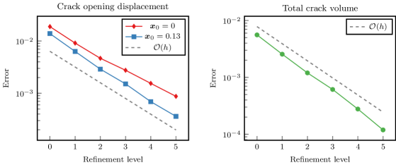
Figure 1: Crack opening displacement convergence for Sneddon’s test computed computed using 3.

4.2 Example 2: Modified Sneddon test with Algorithm 1

We consider a set-up inspired by the previous example, but including Algorithm 1 in a stationary setting. That is, we iterate between the phase-field and FSI problems, thereby coupling the stationary phase-field problem to the pressure resulting from the FSI problem.

4.2.1 Configuration

The spatial configuration is as in the previous example. The stationary Stokes FSI 4 is driven by the right-hand side forcing term

$$\hat{\bm{f}}=c_{1}\exp(-c_{2}((x-x_{0})^{2}+(y-y_{0})^{2}))\bm{e}_{x},$$

with $c_{1}=0.02,c_{2}=1000$ and $(x_{0},y_{0})=(l_{0}/4,2a/3)$ where $l_{0}=0.2$ is the half length of the crack and $a>0$ is the half-height of the resulting ellipse shaped crack, i.e., $\operatorname{cod}(0)/2$. This results in a negative pressure at the left tip and a positive pressure at the right crack tip. Consequently, we expect the crack resulting from the coupled computation to be smaller on the left end of the crack and wider towards the right of the crack. The material parameters for the fluid are $\nu_{f}=0.1$ and $\rho_{f}=10^{3}$. Finally, we choose the harmonic mesh extension parameter as $\alpha_{u}=10^{-14}$.

In order to see the effects of the averaged FSI pressure $p^{*}$ on the phase-field problem, we chose the data as $E=10^{2}$ and $p=4.5$. Consequently, the resulting crack shape is identical to the previous example if the FSI pressure is ignored.

4.2.2 Results

The resulting crack shape on the two finest meshes (four and five levels of mesh refinement, respectively) from the coupled FSI pressure and Sneddon background pressure can be seen on the left of Figure 2 (solid lines) together with the resulting Sneddon crack, i.e., no FSI pressure (dashed lines). On the right of Figure 2, we show the FSI pressure inside the reconstructed crack. We observe that where the FSI pressure is positive, the resulting crack is larger than the Sneddon crack, and where it is negative, the COD is smaller, as is to be expected.

In Figure 3, we see the convergence of the crack opening displacements in the points $x=0$ and $x=0.13$, as well as the convergence of the total crack volume towards the reference value. The reference value is the result computed on the fines mesh (five levels of mesh refinement). We again observe approximately linear mesh convergence for all three quantities.

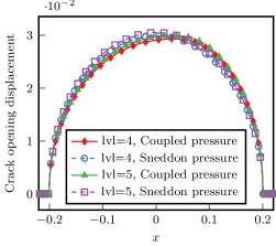
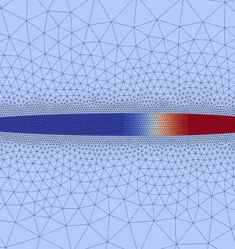
Figure 2: Example 2: Fluid-filled phase-field crack coupled with the fluid-structure-interaction pressure. Left: Resulting crack shape based on the crack opening displacements after four sub-iterations between the phase-field and the fluid-structure-interaction problem with $lvl\in\{4,5\}$ levels of mesh refinement. Right: Fluid-Structure interaction pressure on the reconstructed domain used to drive the divergence from Sneddon’s test on mesh level three.

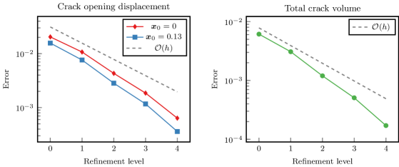
Figure 3: Example 2: Fluid-filled phase-field crack coupled with the fluid-structure-interaction pressure. Left: Numerical convergence for the crack opening displacements in two points. Right: Numerical convergence of the total crack volume.

4.3 Example 3: Crack starting from a boundary with fluid flow boundary conditions

In this example, we consider a crack from the boundary of the domain, rather than a crack fully contained in the domain. This contact of the crack domain with the boundary adds technical challenges to the reconstruction procedure.

4.3.1 Configuration

The domain of interest is $\Omega=(-1,1)^{2}$. The initial crack is given by $\pazocal{C}_{0}=(-1,0)\times(-h,h)$. The mechanical parameters are $E_{s}=5\cdot 10^{4}$ and $\nu_{s}=0.35$. We choose the model parameters in the phase-field problem as $G_{c}=500$, $\kappa=10^{-10}$, $\gamma=100h^{-2}$, and $\varepsilon=2h$. The phase-field background pressure is $10^{3}$.

In contrast to the previous examples, the crack touches the outer boundary. Therefore, we have to proceed non-homogeneous Dirichlet boundary conditions for the deformation field. Following [21, Section 6.3] these are given as $\bm{u}_{x}=0$, and

$$\bm{u}_{y}=\begin{cases}c\sqrt{\sqrt{x^{2}+y^{2}}-x}&\text{if }y>0\\ -c\sqrt{\sqrt{x^{2}+y^{2}}-x}&\text{if }y\leq 0,\end{cases}$$

with $c=0.08/\sqrt{2}$. For the phase-field, we again have homogenous Neumann boundary conditions.

As the crack touches the outer boundary, we can also consider a different set-up for the fluid-structure interaction problem. Rather than specifying a volume force, we specify an inflow boundary condition on the outer boundary of the open crack. Specifically, we set

$$\hat{\bm{v}}_{f}=\begin{pmatrix}v_{\text{max}}(d/2-y)(d/2+y)/d^{2}\\ 0\end{pmatrix},$$

where $v_{\text{max}}=0.001$ is the maximal inflow speed and $d=\operatorname{cod}(x=-1)$ is the size of the crack opening at the boundary. For the FSI deformation, we set homogeneous Dirichlet Conditions on the top, bottom and inflow boundaries, and homogeneous Neumann boundary conditions on the left and right boundaries. The body forcing term is set as $\hat{\bm{f}}=0$.

4.3.2 Results

We consider $h_{0}=0.01$ and five levels of mesh refinement. The phase-field deformation, together with the computational mesh, and the phase-field solution on mesh level three, can be seen in Figure 4. In particular, we see the expected discontinuity of the vertical component of the deformation along the crack. In Figure 5, we observe the fluid-structure interaction deformation, velocity and pressure on the same mesh level. This particularly illustrates the reconstructed domain and the flexibility regarding the problem posed inside the open crack by the domain reconstruction. Finally, In Figure 6, we again consider the numerical convergence of the $\operatorname{cod}$ and $\operatorname{tcv}$ towards the values resulting from the finest mesh level. We again observe linear convergence, with a slight deviation on mesh level two.

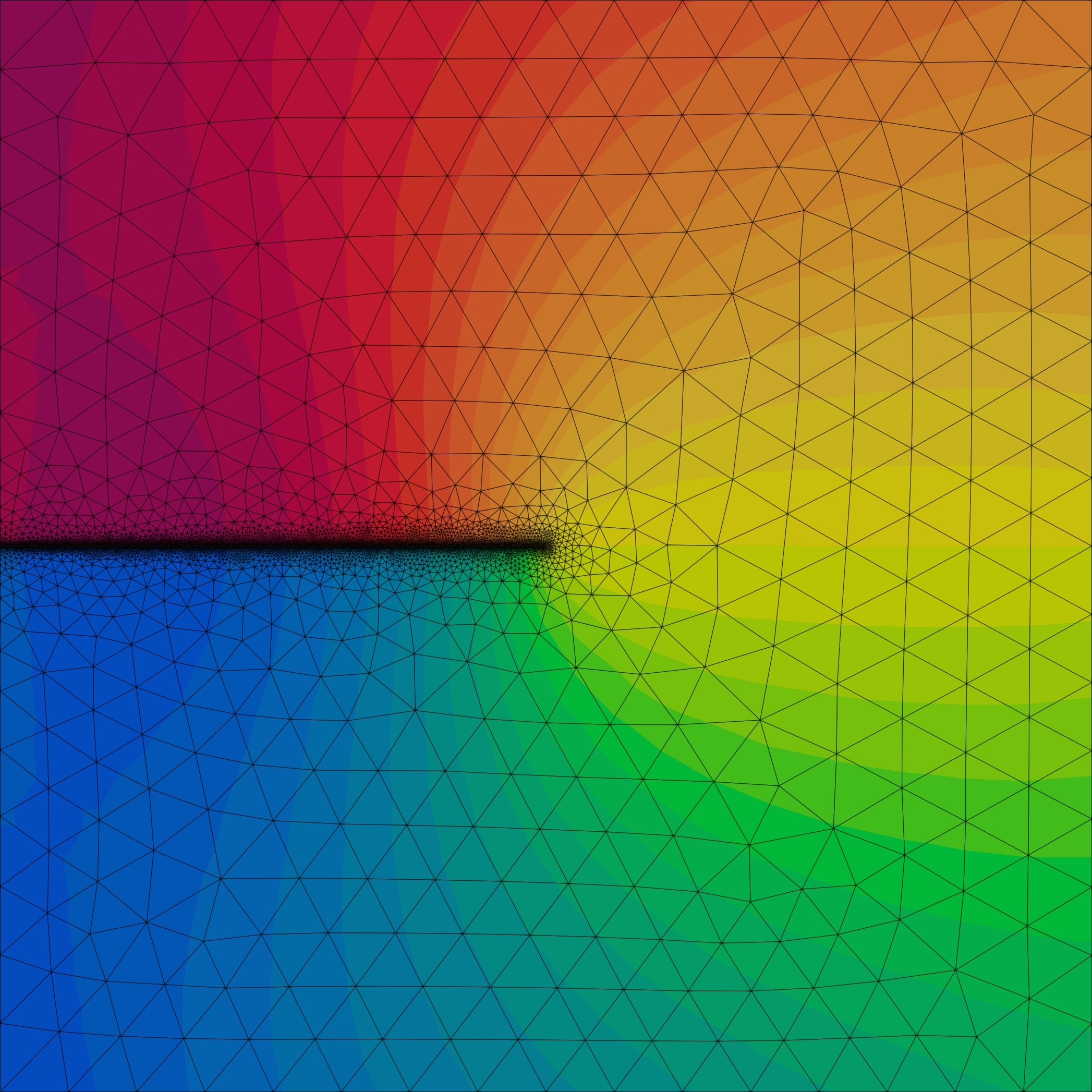
Figure 4: Example 3: Phase-field-deformation (vertical component) and phase-field after three levels of mesh refinement.

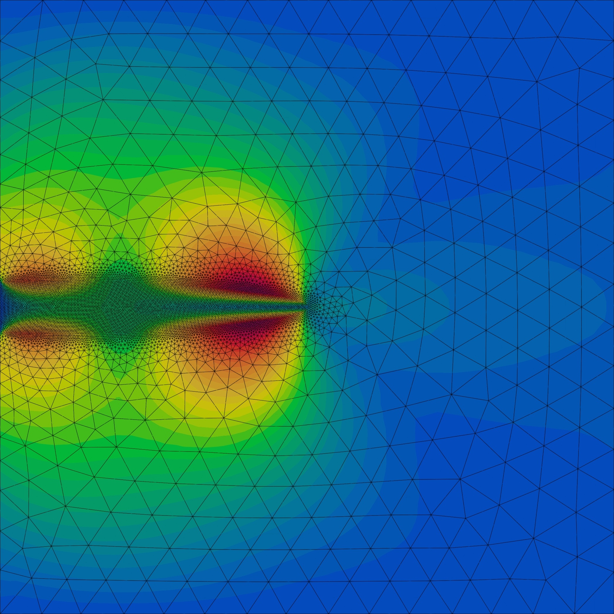
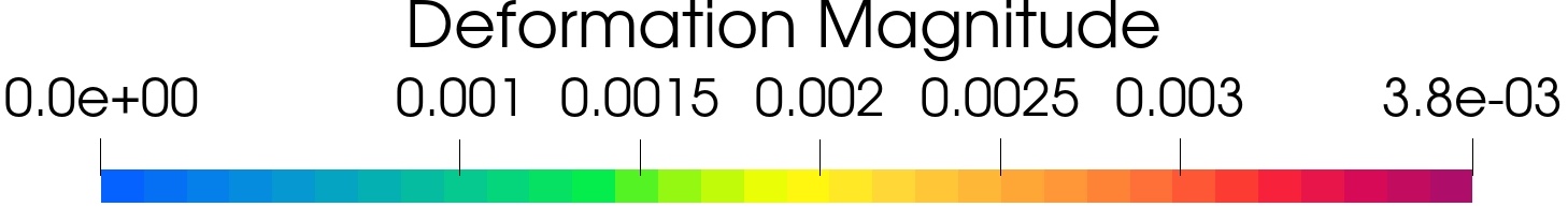
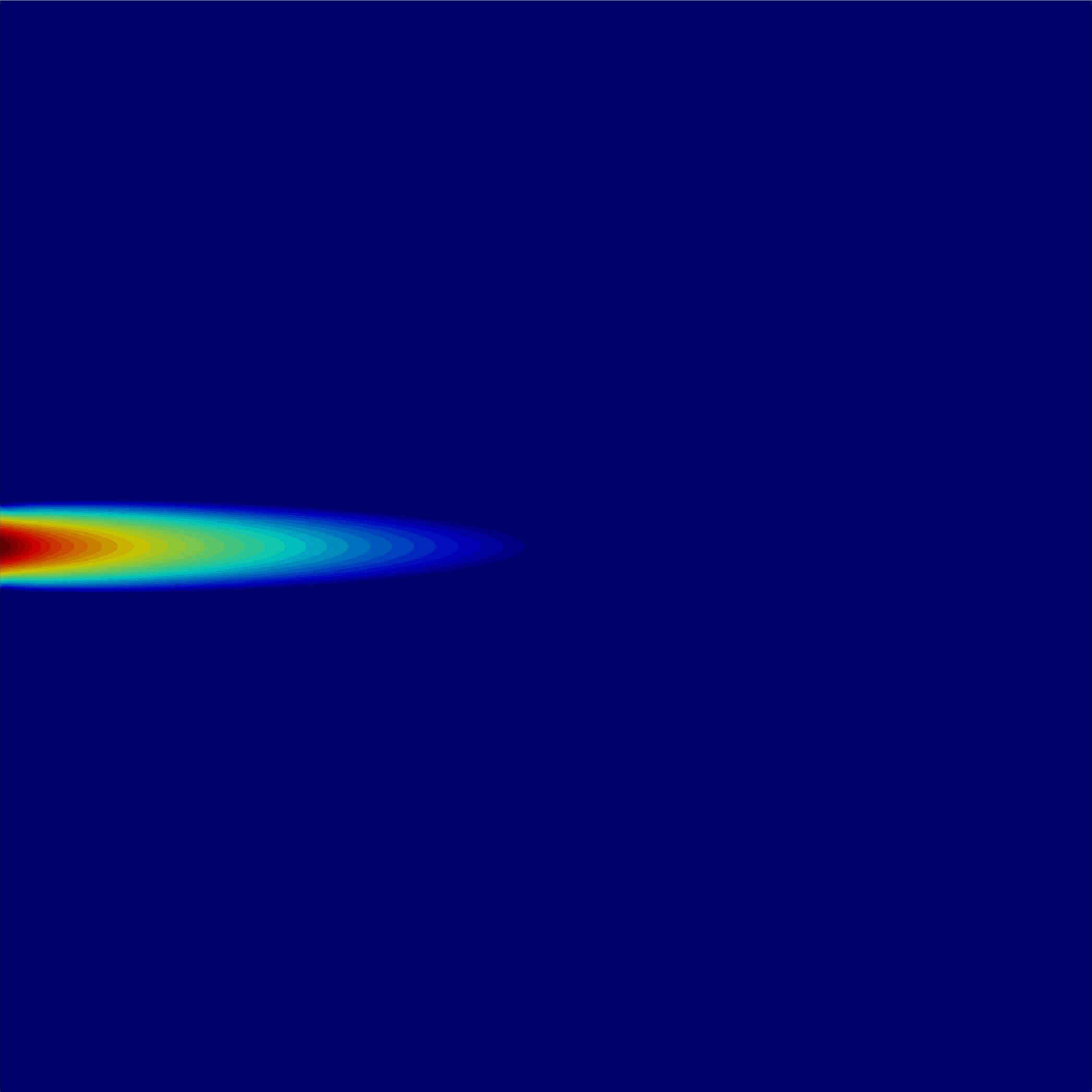
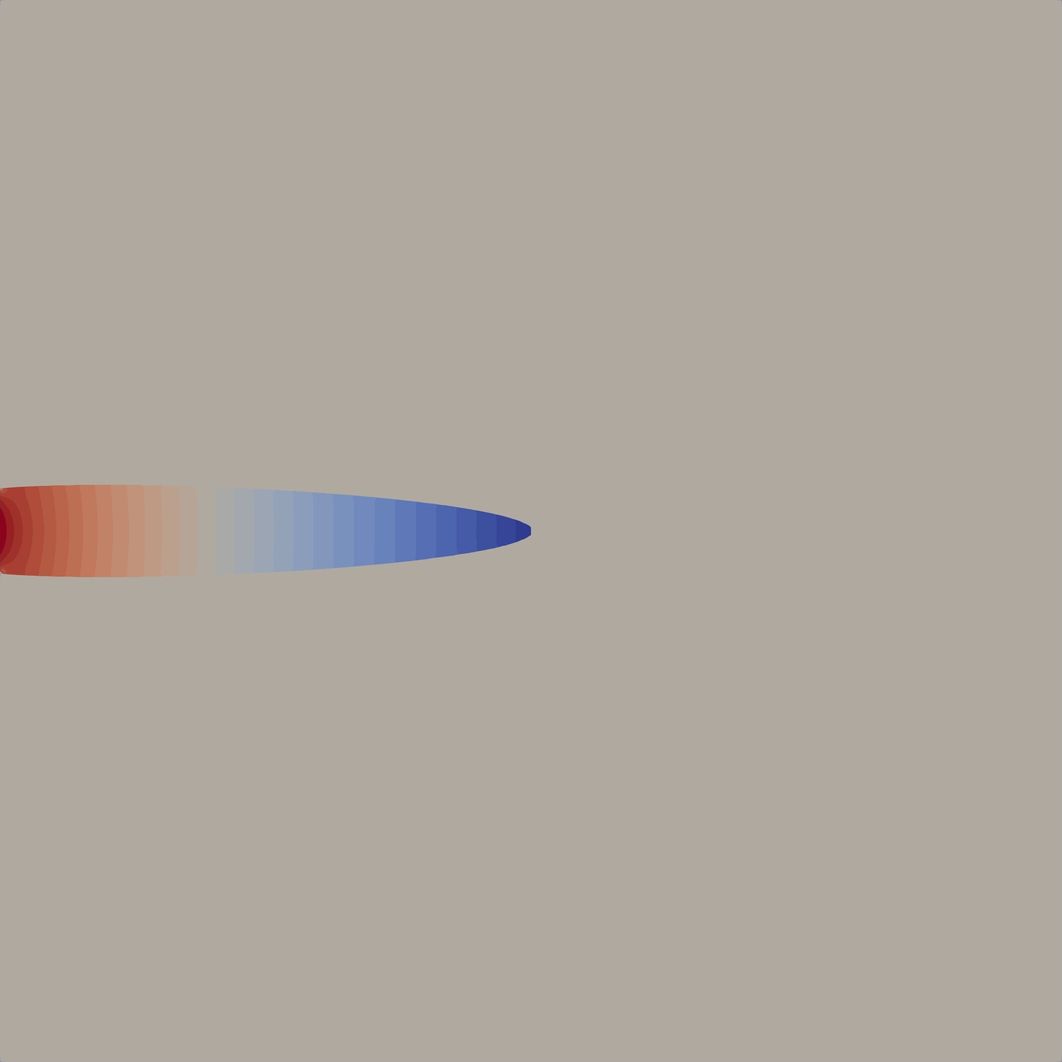
Figure 5: Example 3: FSI-deformation magnitude, velocity magnitude and FSI-pressure after three levels of mesh refinement.

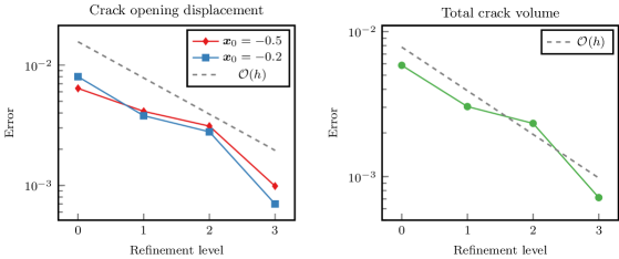
Figure 6: Example 3: Convergence of $\operatorname{cod}$ and $\operatorname{tcv}$ on different spatial refinement levels.

4.4 Example 4: A propagating fracture

We extend the previous examples by considering an incrementally-increasing, pressure resulting in a growing crack.

4.4.1 Configuration

The domain of interest is again $\Omega=(-2,2)^{2}$. The mechanical parameters are as in Example 1, that is, $E_{s}=10^{5}$ and $\nu_{s}=0.35$. We choose the model parameters in the phase-field problem as $G_{c}=500$, $\kappa=10^{-10}$, $\gamma=100h^{-2}$, while we take the phase-field regularisation parameter fixed as $\varepsilon=0.04$. This is because we cannot expect mesh convergence in this setting with varying $\varepsilon$ [74, 39].

The time-dependent background pressure driving the growing crack is

$$p(t)=4500+10t\qquad\text{for }t\in[0,0.5].$$

We take the constant time step $\Delta t=0.1$. In each time steps, we again use five iterations so solve the phase-field problem.

For the fluid-structure interaction problem, we take the right-hand side $\hat{\bm{f}}=(5,0)^{T}$. In a pure fluid flow problem, this would be a no-flow problem. But even in the FSI context, this results in a large pressure. We chose this as only the pressure couples back to the phase-field problem, and we need a sufficiently large pressure to have an impact on the dynamics of the phase-field problem. With our given right-hand side forcing term, the pressure difference between the left an right tip is about $2\cdot 10^{3}$.

4.4.2 Results

The phase-field solution on meshes with $h_{\text{crack}}=0.004,0.002,0.001$ is shown in Figure 7. The temporal behaviour of the crack tip is plotted in Figure 8. Furthermore, at $t=1$, the left mesh tip is at $x=-0.21625492$, $-0.29008647$, $-0.34273292$ and the right tip at $x=0.47777961$, $0.54183778$, $0.49064490$ on the three meshes respectively. As expected, the crack grows faster towards the right, where the total pressure is larger than on the left due to the coupled FSI pressure. While the crack appears to grow only marginally on the coarsest mesh, the results are consistent on the two finer meshes.

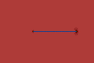
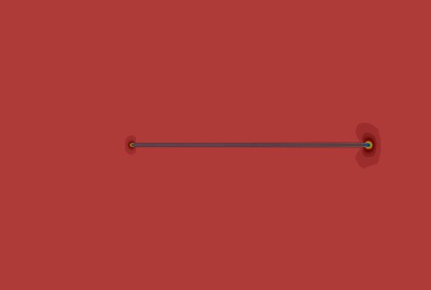
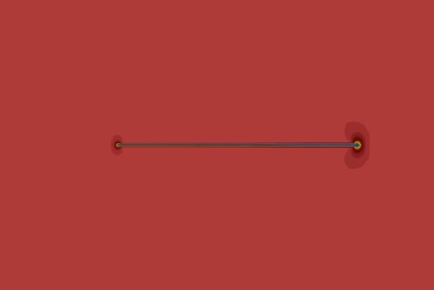
Figure 7: Example 4: Phase-field solution at $t=0.5$ over three meshes in the region $(-0.75,0.75)\times(-0.5,0.5)$.

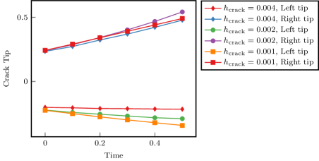
Figure 8: Example 4: Crack tips over time.

5 Conclusions

In this work, we designed and tested a fully coupled algorithm for iterating between phase-field fracture and fluid-structure interaction. More specifically, we first designed a pressurized phase-field approach including the interface conditions stated explicitly on the boundary of the crack domain to compute the fracture path or fracture propagation. This is motivated by the fact that the fluid-structure interaction pressure, used to couple the FSI and phase-field models, only exists inside the fluid-filled crack and not the entire domain.

Next, we used the fracture displacements resulting from the phase-field model to reconstruct the mesh to distinguish between the fluid-filled fracture domain and the surrounding medium by a sharp interface. With the reconstructed mesh, we used the well-known interface-tracking approach (ALE) to solve the fluid-structure interaction problem. This allowed us to solve, for example, Stokes flow in the fracture domain, driven by both volumetric forcing or prescribed boundary conditions. The resulting pressure is applied to the pressurized phase-field fracture sub-problem, which allowed us to couple the two sub-problems iteratively.

We substantiated our final algorithm with numerical experiments in which we undertook both quantitative studies, in terms of computational convergence studies, and observed qualitative behaviour of the solution. The current findings are promising and give hope to extend this in further studies to fully time-dependent problems. However, for the latter, the entire model must be updated, including time-dependent terms, which are planned as future work.

Data Availability Statement

The source code and the data generated with it is publicly available on github under https://github.com/hvonwah/repro-coupled-phase-field-fsi and archived on zenodo [84].

References

- [1] Henry Wahl and Thomas Wick “A high-accuracy framework for phase-field fracture interface reconstructions with application to Stokes fluid-filled fracture surrounded by an elastic medium” In Comput. Methods Appl. Mech. Engrg. 415, 2023, pp. 116202 DOI: 10.1016/j.cma.2023.116202
- [2] K. Yoshioka, D. Naumov and O. Kolditz “On crack opening computation in variational phase-field models for fracture” In Comput. Methods Appl. Mech. Engrg. 369 Elsevier BV, 2020, pp. 113210 DOI: 10.1016/j.cma.2020.113210
- [3] B. Giovanardi, A. Scotti and L. Formaggia “A hybrid XFEM –Phase field ( Xfield ) method for crack propagation in brittle elastic materials” In Comput. Methods Appl. Mech. Engrg. 320 Elsevier BV, 2017, pp. 396–420 DOI: 10.1016/j.cma.2017.03.039
- [4] Yongxiang Wang and Haim Waisman “From diffuse damage to sharp cohesive cracks: A coupled XFEM framework for failure analysis of quasi-brittle materials” In Comput. Methods Appl. Mech. Engrg. 299, 2016, pp. 57–89 DOI: 10.1016/j.cma.2015.10.019
- [5] Yue Xu, Tao You and Qizhi Zhu “Reconstruct lower-dimensional crack paths from phase-field point cloud” In International Journal for Numerical Methods in Engineering 124.15, 2023, pp. 3329–3351 DOI: https://doi.org/10.1002/nme.7249
- [6] T.. Nguyen, J. Yvonnet, Q.-Z. Zhu, M. Bornert and C. Chateau “A phase-field method for computational modeling of interfacial damage interacting with crack propagation in realistic microstructures obtained by microtomography” In Comput. Methods Appl. Mech. Engrg. 312, 2016, pp. 567–595 DOI: 10.1016/j.cma.2015.10.007
- [7] S. Lee, M.. Wheeler and T. Wick “Iterative coupling of flow, geomechanics and adaptive phase-field fracture including level-set crack width approaches” In J. Comput. Appl. Math. 314 Elsevier BV, 2017, pp. 40–60 DOI: 10.1016/j.cam.2016.10.022
- [8] Juan Michael Sargado, Eirik Keilegavlen, Inga Berre and Jan Martin Nordbotten “A combined finite element–finite volume framework for phase-field fracture” In Comput. Methods Appl. Mech. Engrg. 373, 2021, pp. 113474 DOI: 10.1016/j.cma.2020.113474
- [9] A. Kumar, B. Bourdin, G.. Francfort and O. Lopez-Pamies “Revisiting nucleation in the phase-field approach to brittle fracture” In J. Mech. Phys. Solids 142, 2020, pp. 104027 DOI: 10.1016/j.jmps.2020.104027
- [10] B. Bourdin, G.. Francfort and J.-J. Marigo “Numerical experiments in revisited brittle fracture” In J. Mech. Phys. Solids 48.4 Elsevier BV, 2000, pp. 797–826 DOI: 10.1016/S0022-5096(99)00028-9
- [11] Charlotte Kuhn and Ralf Müller “A continuum phase field model for fracture” Computational Mechanics in Fracture and Damage: A Special Issue in Honor of Prof. Gross In Eng. Fract. Mech. 77.18, 2010, pp. 3625–3634 DOI: 10.1016/j.engfracmech.2010.08.009
- [12] C. Miehe, F. Welschinger and M. Hofacker “Thermodynamically consistent phase-field models of fracture: variational principles and multi-field FE implementations” In Internat. J. Numer. Methods Engrg. 83, 2010, pp. 1273–1311 DOI: 10.1002/nme.2861
- [13] C. Miehe, M. Hofacker and F. Welschinger “A phase field model for rate-independent crack propagation: Robust algorithmic implementation based on operator splits” In Comput. Methods Appl. Mech. Engrg. 199, 2010, pp. 2765–2778 DOI: 10.1016/j.cma.2010.04.011
- [14] M.. Borden, C.. Verhoosel, M.. Scott, T… Hughes and C.. Landis “A phase-field description of dynamic brittle fracture” In Comput. Methods Appl. Mech. Engrg. 217, 2012, pp. 77–95 DOI: 10.1016/j.cma.2012.01.008
- [15] Marreddy Ambati, Tymofiy Gerasimov and Laura De Lorenzis “A review on phase-field models of brittle fracture and a new fast hybrid formulation” In Comput. Mech. 55.2 Springer Berlin Heidelberg, 2015, pp. 383–405 DOI: 10.1007/s00466-014-1109-y
- [16] Miguel Arriaga and Haim Waisman “Stability analysis of the phase-field method for fracture with a general degradation function and plasticity induced crack generation” IUTAM Symposium on Dynamic Instabilities in Solids In Mech. Mater. 116, 2018, pp. 33–48 DOI: 10.1016/j.mechmat.2017.04.003
- [17] Juan Michael Sargado, Eirik Keilegavlen, Inga Berre and Jan Martin Nordbotten “High-accuracy phase-field models for brittle fracture based on a new family of degradation functions” In J. Mech. Phys. Solids 111, 2018, pp. 458–489 DOI: 10.1016/j.jmps.2017.10.015
- [18] Mary F. Wheeler, Thomas Wick and Sanghyun Lee “IPACS: Integrated Phase-Field Advanced Crack Propagation Simulator. An adaptive, parallel, physics-based-discretization phase-field framework for fracture propagation in porous media” In Comput. Methods Appl. Mech. Engrg. 367, 2020, pp. 113124 DOI: 10.1016/j.cma.2020.113124
- [19] B. Bourdin, G.. Francfort and J.-J. Marigo “The Variational approach to fracture” In J. Elasticity 91.1–3, 2008, pp. 1–148 DOI: 10.1007/s10659-007-9107-3
- [20] J.-Y. Wu et al. “Phase-field modeling of fracture” In Advances in Applied Mechanics Elsevier, 2020, pp. 1–183 DOI: 10.1016/bs.aams.2019.08.001
- [21] T. Wick “Multiphysics Phase-Field Fracture” 28, Radon Series on Computational and Applied Mathematics Berlin, Boston: De Gruyter, 2020 DOI: 10.1515/9783110497397
- [22] Yousef Heider “A review on phase-field modeling of hydraulic fracturing” In Eng. Fract. Mech. 253, 2021, pp. 107881 DOI: 10.1016/j.engfracmech.2021.107881
- [23] Patrick Diehl, Robert Lipton, Thomas Wick and Mayank Tyagi “A comparative review of peridynamics and phase-field models for engineering fracture mechanics” In Comput. Mech. 69, 2022, pp. 1259–1293 DOI: 10.1007/s00466-022-02147-0
- [24] T… Hughes, W.. Liu and T. Zimmermann “Lagrangian-Eulerian finite element formulation for incompressible viscous flows” In Comput. Methods Appl. Mech. Engrg. 29, 1981, pp. 329–349 DOI: 10.1016/0045-7825(81)90049-9
- [25] J. Donea, S. Giuliani and J.. Halleux “An arbitrary Lagrangian-Eulerian finite element method for transient dynamic fluid-structure interactions” In Comput. Methods Appl. Mech. Engrg. 33, 1982, pp. 689–723 DOI: 10.1016/0045-7825(82)90128-1
- [26] J. Donea, A. Huerta, J.-Ph. Ponthot and A. Rodriguez-Ferran “Arbitrary Lagrangian-Eulerian methods”, Encyclopedia of Computational Mechanics John WileySons, 2004, pp. 1–25
- [27] L. Formaggia and F. Nobile “A stability analysis for the Arbitrary Lagrangian Eulerian Formulation with Finite Elements” In East-West J. Numer. Math. 7, 1999, pp. 105–132
- [28] L. Formaggia and F. Nobile “Stability analysis of second-order time accurate schemes for ALE-FEM” In Comput. Methods Appl. Mech. Engrg. 193.39-41, 2004, pp. 4097–4116
- [29] H.-J. Bungartz and M. Schäfer “Fluid-Structure Interaction: Modelling, Simulation, Optimization” 53, Lecture Notes in Computational Science and Engineering Springer, 2006
- [30] H.-J. Bungartz, Miriam Mehl and M. Schäfer “Fluid-Structure Interaction II: Modelling, Simulation, Optimization”, Lecture Notes in Computational Science and Engineering Springer, 2010
- [31] T. Richter “Fluid-structure interactions: Models, analysis, and finite elements” Springer, 2017 DOI: 10.1007/978-3-319-63970-3
- [32] G. Galdi and R. Rannacher “Fundamental Trends in Fluid-Structure Interaction” World Scientific, 2010, pp. 293 DOI: 10.1142/7675
- [33] T. Bodnár, G.. Galdi and Š. Nečasová “Fluid-Structure Interaction and Biomedical Applications”, Advances in Mathematical Fluid Mechanics Springer Basel, 2014
- [34] Y. Bazilevs, K. Takizawa and T.. Tezduyar “Computational Fluid-Structure Interaction: Methods and Applications” Wiley, 2013 DOI: 10.1002/9781118483565
- [35] L. Formaggia, A. Quarteroni and A. Veneziani “Cardiovascular Mathematics: Modeling and simulation of the circulatory system” Springer-Verlag, Italia, Milano, 2009
- [36] Pengtao Sun, Jinchao Xu and Lixiang Zhang “Full Eulerian finite element method of a phase field model for fluid-structure interaction problem” In Comput. & Fluids 90.0, 2014, pp. 1–8 DOI: 10.1016/j.compfluid.2013.11.010
- [37] Xiaoyu Mao and Rajeev Jaiman “An interface and geometry preserving phase-field method for fully Eulerian fluid-structure interaction” In J. Comput. Phys. 476, 2023, pp. 111903 DOI: 10.1016/j.jcp.2022.111903
- [38] T. Wick “Coupling fluid-structure interaction with phase-field fracture” In J. Comput. Phys. 327, 2016, pp. 67–96 DOI: 10.1016/j.jcp.2016.09.024
- [39] A. Mikelić, M.. Wheeler and T. Wick “A phase-field method for propagating fluid-filled fractures coupled to a surrounding porous medium” In SIAM Multiscale Model. Simul. 13.1, 2015, pp. 367–398
- [40] C. Miehe and S. Mauthe “Phase field modeling of fracture in multi-physics problems. Part III. Crack driving forces in hydro-poro-elasticity and hydraulic fracturing of fluid-saturated porous media” In Comput. Methods Appl. Mech. Engrg. 304, 2016, pp. 619–655 DOI: 10.1016/j.cma.2015.09.021
- [41] C. Miehe, S. Mauthe and S. Teichtmeister “Minimization principles for the coupled problem of Darcy–Biot-type fluid transport in porous media linked to phase field modeling of fracture” In J. Mech. Phys. Solids 82, 2015, pp. 186–217 DOI: 10.1016/j.jmps.2015.04.006
- [42] S. Lee, M.. Wheeler and T. Wick “Pressure and fluid-driven fracture propagation in porous media using an adaptive finite element phase field model” In Comput. Methods Appl. Mech. Engrg. 305, 2016, pp. 111–132
- [43] K. Yoshioka and B. Bourdin “A variational hydraulic fracturing model coupled to a reservoir simulator” In Int. J. Rock Mech. Min. Sci. 88, 2016, pp. 137–150 DOI: 10.1016/j.ijrmms.2016.07.020
- [44] Yousef Heider, Sönke Reiche, Philipp Siebert and Bernd Markert “Modeling of hydraulic fracturing using a porous-media phase-field approach with reference to experimental data” In Eng. Fract. Mech. 202, 2018, pp. 116–134 DOI: 10.1016/j.engfracmech.2018.09.010
- [45] T. Cajuhi, L. Sanavia and L. De Lorenzis “Phase-field modeling of fracture in variably saturated porous media” In Comput. Mech. 61.3, 2018, pp. 299–318 DOI: 10.1007/s00466-017-1459-3
- [46] D. Santillan, R. Juanes and L. Cueto-Felgueroso “Phase field model of fluid-driven fracture in elastic media: Immersed-fracture formulation and validation with analytical solutions” 2016JB013572 In J. Geophys. Res. Solid Earth 122.4, 2017, pp. 2565–2589 DOI: 10.1002/2016JB013572
- [47] Zachary A. Wilson and Chad M. Landis “Phase-field modeling of hydraulic fracture” In J. Mech. Phys. Solids 96, 2016, pp. 264–290 DOI: 10.1016/j.jmps.2016.07.019
- [48] Fadi Aldakheel, Nima Noii, Thomas Wick and Peter Wriggers “A global-local approach for hydraulic phase-field fracture in poroelastic media” Robust and Reliable Finite Element Methods in Poromechanics In Comput. Math. Appl. 91, 2021, pp. 99–121 DOI: 10.1016/j.camwa.2020.07.013
- [49] C. Chukwudozie, B. Bourdin and K. Yoshioka “A variational phase-field model for hydraulic fracturing in porous media” In Comput. Methods Appl. Mech. Engrg. 347, 2019, pp. 957–982 DOI: 10.1016/j.cma.2018.12.037
- [50] Yousef Heider and WaiChing Sun “A phase field framework for capillary-induced fracture in unsaturated porous media: drying-induced vs. hydraulic cracking” In Comput. Methods Appl. Mech. Engrg. 359, 2020, pp. 112647\bibrangessep26 DOI: 10.1016/j.cma.2019.112647
- [51] Fan Fei, Andre Costa, John E. Dolbow, Randolph R. Settgast and Matteo Cusini “A phase-field model for hydraulic fracture nucleation and propagation in porous media”, 2023 DOI: 10.48550/arxiv.2304.13197
- [52] Y. Heider and B. Markert “A phase-field modeling approach of hydraulic fracture in saturated porous media” Multi-Physics of Solids at Fracture In Mech. Res. Comm. 80, 2017, pp. 38–46 DOI: 10.1016/j.mechrescom.2016.07.002
- [53] A. Costa, T. Hu and J.. Dolbow “On formulations for modeling pressurized cracks within phase-field methods for fracture” In Theor. Appl. Fract. Mec., 2023, pp. 104040 DOI: 10.1016/j.tafmec.2023.104040
- [54] N. Noii and T. Wick “A phase-field description for pressurized and non-isothermal propagating fractures” In Comput. Methods Appl. Mech. Engrg. 351, 2019, pp. 860–890 DOI: 10.1016/j.cma.2019.03.058
- [55] Cam-Lai Nguyen, Abdel Hassan Sweidan, Yousef Heider and Bernd Markert “Thermomechanical phase-field fracture modeling of fluid-saturated porous media” In Proc. Appl. Math. Mech. 20.1, 2021, pp. e202000332 DOI: 10.1002/pamm.202000332
- [56] Cam-Lai Nguyen, Yousef Heider and Bernd Markert “A non-isothermal phase-field hydraulic fracture modeling in saturated porous media with convection-dominated heat transport” In Acta Geotech., 2023
- [57] H.. Suh and W. Sun “Asynchronous phase field fracture model for porous media with thermally non-equilibrated constituents” In Comput. Methods Appl. Mech. Engrg. 387, 2021, pp. 114182 DOI: 10.1016/j.cma.2021.114182
- [58] S. Badia, A. Quaini and A. Quarteroni “Coupling Biot and Navier–Stokes equations for modelling fluid–poroelastic media interaction” In J. Comput. Phys. 228.21, 2009, pp. 7986–8014 DOI: 10.1016/j.jcp.2009.07.019
- [59] M. Bukač, I. Yotov, R. Zakerzadeh and P. Zunino “Partitioning strategies for the interaction of a fluid with a poroelastic material based on a Nitsche’s coupling approach” Special Issue on Advances in Simulations of Subsurface Flow and Transport (Honoring Professor Mary F. Wheeler) In Comput. Methods Appl. Mech. Engrg. 292, 2015, pp. 138–170 DOI: 10.1016/j.cma.2014.10.047
- [60] M. Bukac, I. Yotov, R. Zakerzadeh and P. Zunino “Effects of Poroelasticity on Fluid-Structure Interaction in Arteries: a Computational Sensitivity Study” In Modeling the Heart and the Circulatory System Springer, 2015, pp. 197–220 DOI: 10.1007/978-3-319-05230-4˙8
- [61] R. Zakerzadeh and P. Zunino “A computational framework for fluid-porous structure interaction with large structural deformation” In Meccanica 54.1-2, 2019, pp. 101–121 DOI: 10.1007/s11012-018-00932-x
- [62] A. Mikelić, M.. Wheeler and T. Wick “A phase-field approach to the fluid filled fracture surrounded by a poroelastic medium” ICES Report 13-15, 2013 URL: www.oden.utexas.edu/media/reports/2013/1315.pdf
- [63] G.. Francfort and J.-J. Marigo “Revisiting brittle fracture as an energy minimization problem” In J. Mech. Phys. Solids 46.8, 1998, pp. 1319–1342 DOI: 10.1016/S0022-5096(98)00034-9
- [64] L. Ambrosio and V.. Tortorelli “Approximation of functionals depending on jumps by elliptic functionals via -convergence” In Comm. Pure Appl. Math. 43.8 Wiley, 1990, pp. 999–1036 DOI: 10.1002/cpa.3160430805
- [65] L. Ambrosio and V.. Tortorelli “On the approximation of free discontinuity problems” In Boll. Un. Mat. Ital. 6, 1992, pp. 105–123
- [66] V. Martin, J. Jaffré and J.. Roberts “Modeling Fractures and Barriers as Interfaces for Flow in Porous Media” In SIAM J. Sci. Comput. 26.5, 2005, pp. 1667–1691 DOI: 10.1137/S1064827503429363
- [67] M. Bukac, I. Yotov and P. Zunino “Dimensional model reduction for flow through fractures in poroelastic media” In ESAIM Math. Model. Numer. Anal. 51.4, 2017, pp. 1429–1471 DOI: 10.1051/m2an/2016069
- [68] A. Mikelić, M.. Wheeler and T. Wick “Phase-field modeling through iterative splitting of hydraulic fractures in a poroelastic medium” In GEM - Int. J. Geomath. 10.1 Springer ScienceBusiness Media LLC, 2019 DOI: 10.1007/s13137-019-0113-y
- [69] B. Bourdin “Image Segmentation with a finite element method” In Mathematical Modelling and Numerical Analysis 33.2, 1999, pp. 229–244
- [70] T.. Nguyen, J. Yvonnet, Q.-Z. Zhu, M. Bornert and C. Chateau “A phase field method to simulate crack nucleation and propagation in strongly heterogeneous materials from direct imaging of their microstructure” In Engineering Fracture Mechanics 139, 2015, pp. 18–39
- [71] Timo Heister and Thomas Wick “Parallel solution, adaptivity, computational convergence, and open-source code of 2d and 3d pressurized phase-field fracture problems” In Proc. Appl. Math. Mech. 18.1 Wiley, 2018, pp. e201800353 DOI: 10.1002/pamm.201800353
- [72] B. Bourdin “Numerical implementation of the variational formulation for quasi-static brittle fracture” In Interfaces and free boundaries 9, 2007, pp. 411–430
- [73] E. Tanné, T. Li, B. Bourdin, J.-J. Marigo and C. Maurini “Crack nucleation in variational phase-field models of brittle fracture” In J. Mech. Phys. Solids 110, 2018, pp. 80–99 DOI: 10.1016/j.jmps.2017.09.006
- [74] T. Heister, M.. Wheeler and T. Wick “A primal-dual active set method and predictor-corrector mesh adaptivity for computing fracture propagation using a phase-field approach” In Comput. Methods Appl. Mech. Engrg. 290 Elsevier BV, 2015, pp. 466–495 DOI: 10.1016/j.cma.2015.03.009
- [75] T. Wick “An Error-Oriented Newton/Inexact Augmented Lagrangian Approach for Fully Monolithic Phase-Field Fracture Propagation” In SIAM J. Sci. Comput. 39.4 Society for Industrial & Applied Mathematics (SIAM), 2017, pp. B589–B617 DOI: 10.1137/16m1063873
- [76] L. Kolditz, K. Mang and T. Wick “A modified combined active-set Newton method for solving phase-field fracture into the monolithic limit” In Comput. Methods Appl. Mech. Engrg. 414 Elsevier BV, 2023, pp. 116170 DOI: 10.1016/j.cma.2023.116170
- [77] A. Mikelić, M.. Wheeler and T. Wick “A quasi-static phase-field approach to pressurized fractures” In Nonlinearity 28.5 IOP Publishing, 2015, pp. 1371–1399 DOI: 10.1088/0951-7715/28/5/1371
- [78] J. Hron and S. Turek “A monolithic FEM/Multigrid solver for ALE formulation of fluid structure with application in biomechanics” Springer, 2006, pp. 146–170 DOI: 10.1007/3-540-34596-5˙7
- [79] T. Dunne “Adaptive Finite Element Approximation of Fluid-Structure Interaction Based on Eulerian and Arbitrary Lagrangian-Eulerian Variational Formulations”, 2007 DOI: 10.11588/heidok.00007944
- [80] T. Wick “Adaptive Finite Element Simulation of Fluid-Structure Interaction with Application to Heart-Valve Dynamics”, 2011 DOI: 10.11588/heidok.00012992
- [81] T. Richter and T. Wick “Finite elements for fluid-structure interaction in ALE and fully Eulerian coordinates” In Comput. Methods Appl. Mech. Engrg. 199, 2010, pp. 2633–2642 DOI: 10.1016/j.cma.2010.04.016
- [82] E. Burman, S. Claus, P. Hansbo, M.. Larson and A. Massing “CutFEM: Discretizing geometry and partial differential equations” In Internat. J. Numer. Methods Engrg. 104.7 Wiley, 2014, pp. 472–501 DOI: 10.1002/nme.4823
- [83] R. Temam “Navier-Stokes Equations: Theory and Numerical Analysis” Providence, Rhode Island: AMS Chelsea Publishing, 2001
- [84] H. Wahl and T. Wick “A coupled high-accuracy phase-field fluid-structure interaction framework for Stokes fluid-filled fracture surrounded by an elastic medium - Reproduction Scripts” Zenodo repository: Zenodo, 2023 DOI: 10.5281/zenodo.8298461
- [85] J. Schöberl “NETGEN an advancing front 2D/3D-mesh generator based on abstract rules” In Comput. Vis. Sci. 1.1 Springer Nature, 1997, pp. 41–52 DOI: 10.1007/s007910050004
- [86] J. Schöberl “C++11 implementation of finite elements in NGSolve”, 2014 URL: http://www.asc.tuwien.ac.at/~schoeberl/wiki/publications/ngs-cpp11.pdf
- [87] C. Lehrenfeld, F. Heimann, J. Preuß and H. Wahl “ngsxfem: Add-on to NGSolve for geometrically unfitted finite element discretizations” In J. Open Source Softw. 6.64 The Open Journal, 2021, pp. 3237 DOI: 10.21105/joss.03237
- [88] I.. Sneddon “The distribution of stress in the neighbourhood of a crack in an elastic solid” In Proc. R. Soc. A 187.1009 The Royal Society, 1946, pp. 229–260 DOI: 10.1098/rspa.1946.0077
- [89] I.. Sneddon and M. Lowengrub “Crack problems in the classical theory of elasticity”, SIAM series in Applied Mathematics Philadelphia: John WileySons, 1969