Ensemble of Counterfactual Explainers

Abstract

In eXplainable Artificial Intelligence (XAI), several counterfactual explainers have been proposed, each focusing on some desirable properties of counterfactual instances: minimality, actionability, stability, diversity, plausibility, discriminative power. We propose an ensemble of counterfactual explainers that boosts weak explainers, which provide only a subset of such properties, to a powerful method covering all of them. The ensemble runs weak explainers on a sample of instances and of features, and it combines their results by exploiting a diversity-driven selection function. The method is model-agnostic and, through a wrapping approach based on autoencoders, it is also data-agnostic.

1 Introduction

In eXplainable AI (XAI), several counterfactual explainers have been proposed, each focusing on some desirable properties of counterfactual instances. Consider an instance $x$ for which a black box decision $b(x)$ has to be explained. It should be possible to find various counterfactual instances $c$ (availability) which are valid (change the decision outcome, i.e., $b(c)\neq b(x)$), minimal (the number of features changed in $c$ w.r.t. $x$ should be as small as possible), actionable (the feature values in $c$ that differ from $x$ should be controllable) and plausible (the feature values in $c$ should be coherent with the reference population). The counterfactuals found should be similar to $x$ (proximity), but also different among each other (diversity). Also, they should exhibit a discriminative power to characterize the black box decision boundary in the feature space close to $x$. Counterfactual explanation methods should return similar counterfactuals for similar instances to explain (stability). Finally, they must be fast enough (efficiency) to allow for interactive usage.

In the literature, these desiderata for counterfactuals are typically modeled through an optimization problem [12], which, on the negative side, favors only a subset of the properties above. We propose here an ensemble of counterfactual explainers (ece) that, as in the case of ensemble of classifiers, boosts weak explainers to a powerful method covering all of the above desiderata. The ensemble runs base counterfactual explainers (bce) on a sample of instances and of features, and it combines their results by exploiting a diversity-driven selection function. The method is model-agnostic and, through a wrapping approach based on encoder/decoder functions, it is also data-agnostic. We will be able to reason uniformly on counterfactuals for tabular data, images, and time series. An extensive experimentation is presented to validate the approach. We compare with state-of-the-art explanation methods on several metrics from the literature.

2 Related Work

Research on XAI has flourished over the last few years [5]. Explanation methods can be categorized as: (i) intrinsic vs post-hoc, depending on whether the AI model is directly interpretable, or if the explanation is computed for a given black box model; (ii) model-specific vs model-agnostic, depending on whether the approach requires access to the internals of the black box model; (iii) local or global, depending on whether the explanation regards a specific instance, or the overall logic of the black box. Furthermore, explanation methods can be categorized w.r.t. the type of explanation they return (factual or counterfactual) and w.r.t. the type of data they work with. We restrict to local and post-hoc methods returning counterfactual explanations, which is the focus of our proposal.

A recent survey of counterfactual explainers is [15]. Most of the systems are data-specific and generate synthetic (exogenous) counterfactuals. Some approaches search endogenous counterfactuals in a given dataset [9] of instances belonging to the reference population. Exogenous counterfactuals may instead break known relations between features, producing unrealistic instances. Early approaches generated exogenous counterfactuals by solving an optimization problem [12]. In our proposal, we do not rely on this family of methods as they are typically computationally expensive. Another family of approaches are closer to instance-based classification, and rely on a distance function among instances [9, 10]. E.g., [10] grows a sphere around the instance to explain, stopping at the decision boundary of the black box. They are simple but effective, and the idea will be at the core of our base explainers. Some approaches deal with high dimensionality of data through autoencoders [3], which map instances into a smaller latent feature space. Search for counterfactuals is performed in the latent space, and then instances are decoded back to the original space. We rely on this idea to achieve a data-agnostic approach.

3 Problem Setting

A classifier $b$ is a function mapping an instance $x$ from a reference population in a feature space to a nominal value $y$ also called class value or decision, i.e., $b(x)=y$. The classifier $b$ is a black box when its internals are either unknown to the observer or they are known but uninterpretable by humans. Examples include neural networks, SVMs, ensemble classifiers [5].

A counterfactual of $x$ is an instance $c$ for which the decision of the black box differs from the one of $x$, i.e., such that $b(c)\neq b(x)$. A counterfactual is actionable if it belongs to the reference population. Since one may not have a complete specification of the reference population, a relaxed definition of actionability is to require the counterfactual to satisfy given constraints on its feature values. We restrict to simple constraints $a_{A}(c,x)$ that hold iff $c$ and $x$ have the same values over for a set $A$ of actionable features. Non-actionable features (such as age, gender, race) cannot be changed when searching for a counterfactual.

A $k$-counterfactual explainer is a function $f_{k}$ returning a set $C=\{c_{1},\dots,c_{h}\}$ of $h\leq k$ actionable counterfactuals for a given instance of interest $x$, a black box $b$, a set $X$ of known instances from the reference population, and a set $A$ of actionable features, i.e., $f_{k}(x,b,X,A)=C$. For endogenous approaches, $C\subseteq X$. A counterfactual explainer is model-agnostic (resp., data-agnostic) if the definition of $f_{k}$ does not depend on the internals of $b$ (resp., on the data type of $x$). We consider the following data types: tabular data, time series and images. For tabular data, an instance $x=\{(a_{1},v_{1}),\dots,(a_{m},v_{m})\}$ is a tuple of $m$ attribute-value pairs $(a_{i},v_{i})$, where $a_{i}$ is a feature (or attribute) and $v_{i}$ is a value from the domain of $a_{i}$. For example, $x=\{(\mathit{age},22),(\mathit{sex},\mathit{male}),(\mathit{income},\mathit{800})\}$. The domain of a feature can be continuous (age, income), or categorical (sex). For (univariate) time series, an instance $x=\langle v_{1},\dots,v_{m}\rangle$ is an ordered sequence of continuous values (e.g., the body temperature registered at hourly rate). For images, $x$ is a matrix in $\mathbb{R}^{m\times m}$ representing the intensity of the image pixels.

Problem Statement. We consider the problem of designing a $k$-counterfactual explainer satisfying a broad range of properties: availability, validity, actionability, plausibility, similarity, diversity, discriminative power, stability, efficiency.

4 Ensemble of Explainers

Our proposal to the stated problem consists of an ensemble of base explainers named ece (ensamble of counterfactual explainers). Ensemble classifiers boost the performance of weak learner base classifiers by increasing the predictive power, or by reducing bias or variance. Similarly, we aim at improving base $k$-counterfactual explainers by combining them into an ensemble of explainers.

Input : $x$ - instance to explain, $b$ - black box, $X$ - known instances,

$k$ - number of counterfactuals, $A$ - actionable features, $E$ - base explainers

Output : $C$ - $k$-counterfactual set

1 $C\leftarrow\emptyset$; // init. result set

2 for $f_{k}\in E$ do // for each base explainer

3       $X^{\prime}\leftarrow\mathcal{I}(X)$; // sample instances

4       $A^{\prime}\leftarrow\mathcal{F}(A)$; // sample features

5       $C\leftarrow C\cup f_{k}(x,b,X^{\prime},A^{\prime})$; // call base explainer

6      

7$C\leftarrow\mathcal{S}(x,C,k)$; // select top $k$-counterfactuals

8 return $C$;

Algorithm 1 ece

The pseudo-code of ece is shown in Alg. 1. It takes as input an instance to explain $x$, the black box to explain $b$, a set of known instances $X$, the number of required counterfactuals $k$, the set of actionable features $A$, a set of base $k$-counterfactual explainers $E$, and it returns (at most) $k$ counterfactuals $C$. Base explainers are invoked on a sample without replacement $X^{\prime}$ of instances from $X$ (line 3), and on a random subset $A^{\prime}$ of the actionable features $A$ (line 4), as in Random Forests. All counterfactuals produced by the base explainers are collected in a set $C$ (line 5), from which $k$ counterfactuals are selected (line 6). Actionability of counterfactuals is guaranteed by the base explainers (or by filtering out non-actionable ones from their output). Diversity is enforced by randomization (instance and feature sampling) as well as by tailored selection strategies. Stability is a result of combining multiple base explainers, analogously to the smaller variance of ensemble classification w.r.t. the base classifiers. Moreover, if all base explainers are model-agnostic, this also holds for ece.

4.1 Base Explainers

All bce’s presented are parametric to a distance function $d()$ over the feature space. In the experiments, we adopt: for tabular data, a mixed distance weighting Euclidean distance for continuous features and the Jaccard dissimilarity for categorical ones; for images and times series, the Euclidean distance.

Brute Force Explainer (bce-b). A brute force approach considers all subsets $\mathcal{A}$ of actionable features $A$ with cardinality at most $n$. Also, for each actionable feature, an equal-width binning into $r$ bins is computed, and for each bin the center value will be used as representative of the bin. The binning scheme considers only the known instances $X$ with black box decision different from $x$. The brute force approach consists of generating all the possible variations of $x$ with respect to any of the subset in $\mathcal{A}$ by replacing an actionable feature value in $x$ with any representative value of a bin of the feature. Variations are ranked according to their distance from $x$. For each such variation $c$, a $\mathit{refine}$ procedure implements a bisecting strategy of the features in $c$ which are different from $x$ while maintaining $b(c)\neq b(x)$. The procedure returns either a singleton with a counterfactual or an empty set (in case $b(c)=b(x)$). The aim of $\mathit{refine}$ is to improve similarity of the counterfactual with $x$. The procedure stops when $k$ counterfactuals have been found or there is no further candidate. The greater are $n$ and $r$, the larger number of counterfactuals to choose from, but also the higher the computational complexity of the approach, which is $O({|A|\choose n}\cdot n\cdot r)$. bce-b tackles minimization of changes and similarity, but not diversity.

Tree-based Explainer (bce-t). This proposal starts from a (surrogate/shadow [7]) decision tree $\mathcal{T}$ trained on $X$ to mime the black box behavior. Leaves in $T$ leading to predictions different from $b(x)$ can be exploited for building counterfactuals. Basically, the splits on the path from the root to one such leaf represent conditions satisfied by counterfactuals. To ensure actionability, only splits involving actionable constraints are considered. To tackle minimality, the filtered paths are sorted w.r.t. the number of conditions not already satisfied by $x$. For each such path, we choose one instance $c$ from $X$ reaching the leaf and minimizing distance to $x$. Even though the path has been checked for actionable splits, the instance $c$ may still include changes w.r.t. $x$ that are not actionable. For this, we overwrite non-actionable features. Since not all instances at a leaf have the same class as the one predicted at the leaf, we also have to check for validity before including $c$ in the result set. The search over different paths of the decision tree allows for some diversity in the results, even though this cannot be explicitly controlled for. The computational complexity requires both a decision tree construction and a number of distance calculations.

Generative Sphere-based Explainer (bce-s). The last base counterfactual explainer relies on a generative approach growing a sphere of synthetic instances around $x$ [10]. Instance are generated in all directions of the feature space until the decision boundary of the black box $b$ is crossed and the closest counterfactual to $x$ is retrieved. The sphere radius is initialized to a large value, and then it is decreased until the boundary is crossed. Next, a lower bound radius and an upper bound radius are determined such that the boundary of $b$ crosses the area of the sphere between the lower bound and the upper bound radii. In its original version, the growing spheres algorithm generates instances following a uniform distribution. bce-s adopts instead a Gaussian-Matched generation [1]. To ensure actionability, non-actionable features of generated instances are set as in $x$. Finally, bce-s selects from the instances in the final ring the ones which are closest to $x$ and are valid. The complexity of the approach depends on the distance of the decision boundary from $x$, which in turn determines the number of iterations needed to compute the final ring.

4.2 Counterfactual Selection

The selection function $\mathcal{S}$ at line 5 of Alg. 1 selects $k$-counterfactuals from those returned by the base explainers. This problem can be formulated as maximizing an objective function over $k$-subsets of valid counterfactuals $C$. We adopt a density-based objective function:

$$\underset{S\subseteq C\wedge|S|\leq k}{\operatorname*{arg\,max}}\ |\bigcup_{c\in S}\mathit{knn}_{C}(c)|-\lambda\sum_{c\in S}d(c,x)$$

It aims at maximizing the difference between the size of neighborhood instances of the counterfactuals (a measure of diversity) and the total distance from $x$ (a measure of similarity) regularized by a parameter $\lambda$. $\mathit{knn}_{C}(c)$ returns the $h$ most similar counterfactuals to $c$ among those in $C$. We adopt the Cost Scaled Greedy (csg) algorithm [4] for the above maximization problem.

4.3 Counterfactuals for Other Data Types

We enable ece to work on data types other than tabular data by wrapping it around two functions. An encoder $\zeta:\mathbb{D}{\rightarrow}\mathbb{R}^{q}$ that maps an instance from its actual domain $\mathbb{D}$ to a latent space of continuous features, and a decoder $\eta:\mathbb{R}^{q}{\rightarrow}\mathbb{D}$ that maps an instance of the latent space back to the actual domain. Using such functions, any explainer $f_{k}(x,b,X,A)$ can be extended to the domain $\mathbb{D}$ by invoking $\eta(f_{k}(\zeta(x),b^{\prime},\zeta(X),A^{\prime}))$ where the black box in the latent space is $b^{\prime}(x)=b(\eta(x))$. The definition of the actionable features in the latent space $A^{\prime}$ depends on the actual encoder and decoder.

Let us consider the image data type (for time series, the reasoning is analogous). A natural instantiation of the wrapping that achieves dimensionality reduction with a controlled loss of information consists in the usage of autoencoders (AE)  [8]. An AE is a neural network composed by an encoder and a decoder which are trained simultaneously for learning a representation that reduces the dimensionality while minimizing the reconstruction loss. A drawback of this approach is that we cannot easily map actionable feature in the actual domain to features in the latent space (this is a challenging research topic on its own). For this, we set $A^{\prime}$ to be the whole set of latent features and hence, we are not able to deal with actionability constraints.

5 Experiments

Table 1: Datasets description and black box accuracy. $n$ is the no. of instances. $m$ is the no. of features. $m_{con}$ and $m_{cat}$ are the no. of continuous and categorical features respectively. $m_{act}$ is the no. of actionable features. $m_{1h}$ is the total no. of features after one-hot encoding. Rightmost columns report classification accuracy: NN stands for DNN for tabular data, and for CNN for images and time series.

Dataset		$n$	$m$	$m_{con}$	$m_{cat}$	$m_{act}$	$m_{1h}$	$l$	RF	NN
tabular	adult	32,561	12	4	8	5	103	2	.85	.84
	compas	7,214	10	7	3	7	17	3	.56	.61
	fico	10,459	23	23	0	22	-	2	.68	.67
	german	1,000	20	7	13	13	61	2	.76	.81
img	mnist	60k	$28\times 28$	all	0	all	-	10	-	.99
	fashion	60k	$28\times 28$	all	0	all	-	10	-	.97
ts	gunpoint	250	150	all	0	all	-	2	-	.72
	power	1,096	24	all	0	all	-	2	-	.98
	ecg200	200	96	all	0	all	-	2	-	.76

Experimental Settings. We consider a few datasets widely adopted as benchmarks in the literature (see Table 1). There are three time series datasets, two image datasets, and four tabular datasets. For each tabular dataset, we have selected the set $A$ of actionable features, as follows. adult: age, education, marital status, relationship, race, sex, native country; compas: age, sex, race; fico: external risk estimate; german: age, people under maintenance, credit history, purpose, sex, housing, foreign worker.

For each dataset, we trained and explained the following black box classifiers: Random Forest (RF) as implemented by scikit-learn, and Deep Neural Networks (DNN) implemented by keras for tabular datasets, and Convolutional Neural Networks (CNNs) implemented with keras for images and time series. We split tabular datasets into a 70% partition used for the training and 30% used for the test, while image and time series datasets are already released in partitioned files. For each black-box and for each dataset, we performed on the training set a random search with a 5-fold cross-validation for finding the best parameter setting. The classification accuracy on the test set is shown in Table 1 (right).

We compare our proposal against competitors from the state-of-the-art offering a software library that is updated and easy to use. dice [12] handles categorical features, actionability, and allows for specifying the number $k$ of counterfactuals to return. However, it is not model-agnostic as it only deals with differentiable models such as DNNs. The FAT [13] library implements a brute force (bf) counterfactual approach. It handles categorical data but not the number $k$ of desired counterfactuals nor actionability. The ALIBI library implements the counterfactual explainers cem [3, 11], cegp [14] and wach [16]. All of them are designed to explain DNNs, do not handle categorical features and return a single counterfactual, but it is possible to enforce actionability by specifying the admissible feature ranges. Finally, ceml [2] is a model-agnostic toolbox for computing counterfactuals based on optimization that does not handle categorical features and returns a single counterfactual. We also re-implemented the case-based counterfactual explainer (cbce) from [9]. For each tool, we use the default settings offered by the library or suggested in the reference paper. For each dataset, we explain 100 instances $x$ from the test set. The set $X$ of known instances in input to the explainers is the training set of the black box. We report aggregated results as means over the 100 instances, datasets and black boxes.

Evaluation Metrics. We evaluate the performances of counterfactual explainers under various perspectives [12]. The measures reported in the following are stated for a single instance $x$ to be explained, and considering the returned $k$-counterfactual set $C=f_{k}(x,b,X,A)$. The metrics are obtained as the mean value of the measures over all $x$’s to explain.

Size. The number of counterfactuals $|C|$ can be lower than $k$. We define $\mathit{size}=|C|/k$. The higher the better. Recall that by definition of a $k$-counterfactual explainer, any $c\in C$ is valid, i.e., $b(c)\neq b(x)$.

Actionability. It accounts for the counterfactuals in $C$ that can be realized: $\mathit{act}=|\{c\in C\ |\;a_{A}(c,x)\}|/k$. The higher the better.

Implausibility. It accounts for how close are counterfactuals to the reference population. It is the average distance of $c\in C$ from the closest instance in the known set $X$. The lower the better.

$$\mathit{impl}=\frac{1}{|C|}\sum_{c\in C}\min_{x\in X}d(c,x)$$

Dissimilarity. It measures the proximity between $x$ and the counterfactuals in $C$. The lower the better. We measure it in two fashions. The first one, named $\mathit{dis_{dist}}$, is the average distance between $x$ and the counterfactuals in $C$. The second one, $\mathit{dis_{count}}$, quantifies the average number of features changed between a counterfactual $c$ and $x$. Let $m$ be the number of features.

$$\mathit{dis_{dist}}=\frac{1}{|C|}\sum_{c\in C}d(x,c)\quad\quad\mathit{dis_{count}}=\frac{1}{|C|m}\sum_{c\in C}\sum_{i=1}^{m}\mathbb{1}_{c_{i}\neq x_{i}}$$

Diversity. It accounts for a diverse set of counterfactuals, where different actions can be taken to recourse the decision of the black box. The higher the better. We denote by $\mathit{div_{dist}}$ the average distance between the counterfactuals in $C$, and by $\mathit{div_{count}}$ the average number of different features between the counterfactuals.

$$\mathit{div_{dist}}=\frac{1}{|C|^{2}}\sum_{c\in C}\sum_{c^{\prime}\in C}d(c,c^{\prime})\quad\quad\mathit{div_{count}}=\frac{1}{|C|^{2}m}\sum_{c\in C}\sum_{c^{\prime}\in C}\sum_{i=1}^{m}\mathbb{1}_{c_{i}\neq c^{\prime}_{i}}$$

Discriminative Power. It measures the ability to distinguish through a naive approach between two different classes only using the counterfactuals in $C$. In line with [12], we implement it as follows. The sets $X_{=}\subset X$ and $X_{\neq}\subset X$ such that $b(X_{=})=b(x)$ and $b(X_{\neq})\neq b(x)$ are selected such that the instances in $X_{=},X_{\neq}$ are the $k$ closest to $x$. Then we train a simple 1-Nearest Neighbor (1NN) classifier using $C\cup\{x\}$ as training set, and $d$ as distance function. The choice of 1NN is due to its simplicity and connection to human decision making starting from examples. We classify the instances in $X_{=}\cup X_{\neq}$ and we use the accuracy of the 1NN as discriminative power ($\mathit{dipo}$).

Instability. It measures to which extent the counterfactuals $C$ are close to the ones obtained for the closest instance to $x$ in $X$ with the same black box decision. The rationale is that similar instances should obtain similar explanations [6]. The lower the better.

$$\mathit{inst}=\frac{1}{1+d(x,x^{\prime})}\frac{1}{|C||C^{\prime}|}\sum_{c\in C}\sum_{c^{\prime}\in C^{\prime}}d(c,c^{\prime})$$

with $x^{\prime}=\mathit{argmin}_{x_{1}\in X\setminus\{x\},b(x_{1})=b(x)}\,d(x,x_{1})$ and $C^{\prime}=f_{k}(x^{\prime},b,X,A)$.

Runtime. It measures the elapsed time required by the explainer to compute the counterfactuals. The lower the better. Experiments were performed on Ubuntu 20.04 LTS, 252 GB RAM, 3.30GHz x 36 Intel Core i9.

In line with [16, 12], in the above evaluation measures, we adopt as distance $d$ the following mixed distance:

$$d(a,b)=\frac{1}{m_{con}}\sum_{i\in\mathit{con}}\frac{|a_{i}-b_{i}|}{\mathit{MAD}_{i}}+\frac{1}{m_{cat}}\sum_{i\in\mathit{cat}}\mathbb{1}_{a_{i}\neq b_{i}}$$

where $\mathit{con}$ (resp., $\mathit{cat}$) is the set of continuous (resp., categorical) feature positions. Such a distance is not necessarily the one used by the compared explainers. In particular, it substantially differs from the one used by ece.

Parameter Tuning. From an experimental analysis (not reported here) of the impact of the components of ece, we set: for bce-b, $r=10$ and $n=1$; and for ece, $|E|=10$ base explainers chosen uniformly random.

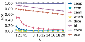
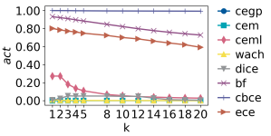
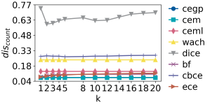
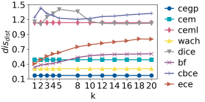
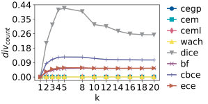
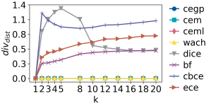
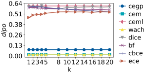
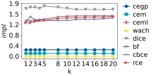
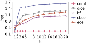
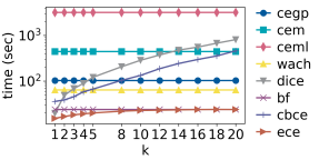
Figure 1: Aggregate metrics on tabular datasets by varying $k$.

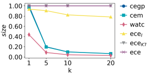
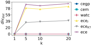
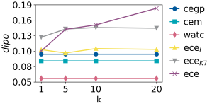
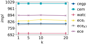
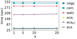
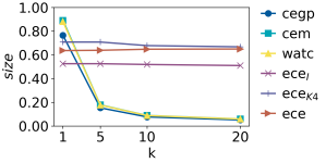
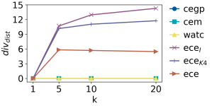
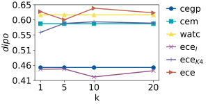
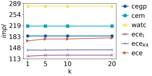
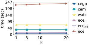
Figure 2: Aggregate metrics on images ($1^{\mathit{st}}$ row) and time series ($2^{\mathit{nd}}$ row) by varying $k$.

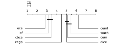
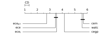
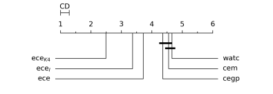
Figure 3: Critical Difference (CD) diagrams for the post-hoc Nemenyi test at 95% confidence level: tabular (left), images (center), and time series (right) datasets.

Quantitative Evaluation. Fig. 1 shows the performance of the compared explainers on tabular data when varying $k$. From the first plot, we notice that only ece, dice, cbce and bf are able to return at least 80% of the required counterfactuals. Most of the other methods only return a single one. From the second plot, we conclude that only ece, bf and cbce return a notable fraction of actionable counterfactuals ($\mathit{act}$). From the plots on dissimilarity ($\mathit{dis}_{count}$ and $\mathit{dis}_{dist}$) and diversity ($\mathit{div}_{count}$ and $\mathit{div}_{dist}$), it turns out that cbce (and also dice) has good values of diversity, but performs poorly w.r.t. dissimilarity. bf wins over ece w.r.t. the $\mathit{dis}_{dist}$ measure, loses w.r.t. the $\mathit{div}_{dist}$ measure, and is substantially equivalent w.r.t. the other two measures. As for discriminative power $\mathit{dipo}$, ece performs slightly lower than dice, cbce, bf and ceml. Regarding plausibility ($\mathit{impl}$), ece is the best performer if we exclude methods that return a single counterfactual (i.e., cem, cegp and wach). Indeed, ece $\mathit{impl}$ is constantly smaller that dice and bf and in line with cbce, which is the only endogenous methods compared. Intuitively, counterfactuals returned by ece resemble instances from the reference population. Concerning instability $\mathit{inst}$, ece is slightly worse than bf and slightly better than dice. ceml is the most stable, and cbce the most unstable. cem, cegp and wach are not shown in the instability plot because, in many cases, they do not return counterfactuals for both of the two similar instances. Finally, all the explainers, with the exception of bf and ece, require on average a runtime of more than one minute. We summarize the performances of the approaches by the CD diagram in Fig. 3 (left), which shows the mean rank position of each method over all experimental runs (datasets $\times$ black boxes $\times$ metrics $\times$ $k$). Overall, ece performs better than all competitors, and the difference is statistically significant.

Fig. 2 shows the performance on images (first row) and time series (second row) datasets. We consider also the ece with the identity encoder/decoder (named ece_I), and with the kernel encoder/decoder (ece_K7 for kernel of size $7\times 7$ and ece_K4 for kernel of size $4\times 4$). For images, cem, cegp and wach return only a single counterfactual, while ece provides more alternatives and with the best diversity. wach returns the least implausible counterfactuals, the variants of ece stand in the middle, while cem returns less realistic counterfactuals. Regarding running time, cegp is the most efficient together with ece_I and ece_K4. The usage of the autoencoder in ece increases the runtime. cem and wach are the slowest approaches. Similar results are observed for time series, with few differences. The CD diagrams in Fig. 3 (center, right) confirm that ece and its variants are the best performing methods.

Acknowledgment. Work partially supported by the European Community H2020-EU.2.1.1 programme under the G.A. 952215 Tailor.

References

- [1] Agustsson, E., et al.: Optimal transport maps for distribution preserving operations on latent spaces of generative models. In: ICLR. OpenReview.net (2019)
- [2] Artelt, A.: Ceml: Counterfactuals for explaining machine learning models - a Python toolbox. https://www.github.com/andreArtelt/ceml (2019 - 2021)
- [3] Dhurandhar, A., et al.: Explanations based on the missing: Towards contrastive explanations with pertinent negatives. In: NeurIPS. pp. 592–603 (2018)
- [4] Ene, A., Nikolakaki, S.M., Terzi, E.: Team formation: Striking a balance between coverage and cost. arXiv:2002.07782 (2020)
- [5] Guidotti, R., Monreale, A., Ruggieri, S., Turini, F., Giannotti, F., Pedreschi, D.: A survey of methods for explaining black box models. CSUR 51(5), 1–42 (2018)
- [6] Guidotti, R., Ruggieri, S.: On the stability of interpretable models. In: IJCNN. pp. 1–8. IEEE (2019)
- [7] Guidotti, R., et al.: Factual and counterfactual explanations for black box decision making. IEEE Intell. Syst. 34(6), 14–23 (2019)
- [8] Hinton, G.E., Salakhutdinov, R.R.: Reducing the dimensionality of data with neural networks. Science 313(5786), 504–507 (2006)
- [9] Keane, M.T., Smyth, B.: Good counterfactuals and where to find them. In: ICCBR. LCNS, vol. 12311, pp. 163–178. Springer (2020)
- [10] Laugel, T., Lesot, M., Marsala, C., Renard, X., Detyniecki, M.: Comparison-based inverse classification for interpretability in machine learning. In: IPMU. pp. 100–111. Springer (2018)
- [11] Luss, R., et al.: Generating contrastive explanations with monotonic attribute functions. arXiv:1905.12698 (2019)
- [12] Mothilal, R.K., Sharma, A., Tan, C.: Explaining machine learning classifiers through diverse counterfactual explanations. In: FAT*. pp. 607–617 (2020)
- [13] Sokol, K., et al.: FAT forensics: A python toolbox for implementing and deploying fairness, accountability and transparency algorithms in predictive systems. J. Open Source Softw. 5(49), 1904 (2020)
- [14] Van Looveren, A., et al.: Interpretable counterfactual explanations guided by prototypes. arXiv:1907.02584 (2019)
- [15] Verma, S., Dickerson, J.P., Hines, K.: Counterfactual explanations for machine learning: A review. arXiv:2010.10596 (2020)
- [16] Wachter, S., et al.: Counterfactual explanations without opening the black box: Automated decisions and the GDPR. Harv. JL & Tech. 31, 841–887 (2017)