ltl_f Best-Effort Synthesis in Nondeterministic
Planning Domains

Abstract

We study best-effort strategies (aka plans) in fully observable nondeterministic domains (FOND) for goals expressed in Linear Temporal Logic on Finite Traces (ltl_f). The notion of best-effort strategy has been introduced to also deal with the scenario when no agent strategy exists that fulfills the goal against every possible nondeterministic environment reaction. Such strategies fulfill the goal if possible, and do their best to do so otherwise. We present a game-theoretic technique for synthesizing best-effort strategies that exploit the specificity of nondeterministic planning domains. We formally show its correctness and demonstrate its effectiveness experimentally, exhibiting a much greater scalability with respect to a direct best-effort synthesis approach based on re-expressing the planning domain as generic environment specifications.

1 Introduction

Recently there has been quite some interest in synthesis [27, 21] for realizing goals (or tasks) $\varphi$ against environment specifications $\mathcal{E}$ [3, 4], especially when both $\varphi$ and $\mathcal{E}$ are expressed in Linear Temporal Logic on finite traces (ltl_f) [19, 20], the finite trace variant of ltl [28], a logic specification language that is commonly adopted in Formal Methods [6]. In this setting, synthesis amounts to finding an agent strategy that wins, i.e., generates a trace satisfying $\varphi$, whatever is the (counter-)strategy chosen by the environment, which in turn has to satisfy its specification $\mathcal{E}$. This form of synthesis can be seen as an extension of FOND planning [23, 24], as shown in, e.g., [18, 10].

Obviously, a winning strategy for the agent may not exist. To handle this possibility, the notion of strong cyclic plans was introduced [12, 11]: if a (strong) plan does not exist, there may still exist a plan that could win assuming the environment is not strictly adversarial. Building on this intuition, Aminof et al. [1] proposed the notion of best-effort strategies (or plans), which formally capture the idea that the agent could do its best by adopting a strategy that wins against a maximal set (though not all) of possible environment strategies. It was then shown in [5] that best-effort strategies capture the game-theoretic rationality principle that a player (the agent) would not use a strategy that is “dominated” by another one (i.e., if another strategy fulfills the goal against more environment behaviors, then the player should adopt that strategy). Best-effort strategies have some notable properties: (i) they always exist, (ii) if a winning strategy exists, then best-effort strategies are exactly the winning strategies, (iii) best-effort strategies can be computed in 2EXPTIME as winning strategies (best-effort synthesis is indeed 2EXPTIME-complete).

In [5] an algorithm for ltl_f best-effort synthesis has been presented. This algorithm is based on creating, solving, and combining the solutions of three distinct games (with three different objectives) played in the same game arena. The arena is obtained from the deterministic finite-state automata (DFAs) corresponding to the ltl_f specification of the agent goal $\varphi$ and the ltl_f specification of the environment $\mathcal{E}$. As a result, the size of the arena is, in the worst-case, double-exponential both in $\varphi$ and in $\mathcal{E}$. Using this framework, we can also capture best-effort synthesis in nondeterministic planning domains. In particular, one can simply re-express nondeterministic planing domains (FOND) in ltl_f [19, 3, 26] and then use the ltl_f best-effort synthesis approach directly. However, observe that in planning, while the (temporally extended) goal $\varphi$ is typically small, the environment specification $\mathcal{E}$ is large, being the entire planning domain (i.e., a representation of how the world the agent is immersed in works). This observation motivates our paper.

We study ltl_f best-effort synthesis directly in the context of nondeterministic (adversarial) planning domains. Specifically, our contributions are:

• A framework for best-effort synthesis in nondeterministic (adversarial) planning domains;

• A synthesis technique for best-effort synthesis, inspired by the one in [5], that takes full advantage of the specificity of planning domains as environment specifications;

• A symbolic best-effort synthesis algorithm that performs and scales well;

• An empirical evaluation of the practical effectiveness of the approach.

Our results show that computing best-effort strategies for ltl_f goals in nondeterministic domains is much more effective than using ltl_f best-effort synthesis directly. In fact, our technique can be implemented quite efficiently, with only a small overhead wrt to computing winning strategies (i.e., strong plans) in FOND. Hence, it is completely feasible in practice to return a best-effort strategy instead of giving up when a winning strategy does not exist.

Figure 1: An arch. We denote location names in the blocks.

Running Example.  We now present a relatively simple example to illustrate the key structure of ltl_f best-effort synthesis in nondeterministic planning domains. This example, adapted from [26], represents a human-robot co-assembly task in a shared workplace. Specifically, the human and robot involved in the task are considered as the environment and the agent, respectively. In the shared workplace, the robot can perform grasp/place actions to pick/drop blocks and transfer/transit actions to move its robotic arm with/without a block in its gripper. After every robot action, the human can react by also moving blocks among locations to interfere with the robot, hence introducing nondeterminism to robot actions. Consider a robot goal (aka task) of assembling an arch of blocks, as depicted in Figure 1. It is easy to see that the agent has no winning strategy (aka strong solution) to assemble the arch, since the human can always disassemble it. Therefore, standard synthesis [20, 18] would conclude the task as unrealizable, hence “giving up". However, the robot still has the chance to fulfill the goal, should the human cooperate or even perform flawed reactions due to e.g. lack of adequate training. Therefore, instead of simply giving up, the agent should try its best to pursue the goal by exploiting human reactions. Best-effort strategies (aka best-effort solutions) precisely capture this intuition.

2 Preliminaries

Traces. Let $\Sigma$ be a set of propositions. A trace $\pi=\pi_{0}\pi_{1}\ldots$ is a sequence of propositional interpretations (sets), where for every $i\geq 0$, $\pi_{i}\in 2^{\Sigma}$ is the $i$-th interpretation of $\pi$. Intuitively, $\pi_{i}$ is interpreted as the set of propositions that are $true$ at instant $i$. The length of a trace is $|\pi|$. A trace $\pi$ is an infinite trace if $|\pi|=\infty$, which is formally denoted as $\pi\in(2^{\Sigma})^{\omega}$; otherwise $\pi$ is a finite trace, denoted as $\pi\in(2^{\Sigma})^{*}$. If a trace $\pi$ is finite, we denote by $\mathtt{lst}(\pi)$ its last instant (i.e., index). Moreover, by $\pi^{k}=\pi_{0}\cdots\pi_{k}$ we denote the prefix of $\pi$ up to the $k$-th iteration.

LTL_f Basics. Linear Temporal Logic on finite traces (ltl_f) is a specification language to express temporal properties on finite and non-empty traces [19]. In particular, ltl_f has the same syntax as ltl, which is instead interpreted over infinite traces [28]. Given a set of propositions $\Sigma$, ltl_f formulas are generated as follows:

$\varphi::=p\mid\varphi\wedge\varphi\mid\neg\varphi\mid\raisebox{-1.1625pt}{\LARGE$\circ$}\varphi\mid\varphi\mathop{\mathcal{U}}\varphi.$

$p\in\Sigma$ is an atom, $\circ$ (Next), and $\mathop{\mathcal{U}}$ (Until) are temporal operators. We use standard Boolean abbreviations such as $\vee$ (or) and $\supset$ (implies), $\mathit{true}$ and $\mathit{false}$. Moreover, we define the following abbreviations Weak Next $\raisebox{-1.1625pt}{\LARGE$\bullet$}\varphi\equiv\neg\raisebox{-1.1625pt}{\LARGE$\circ$}\neg\varphi$, Eventually $\Diamond\varphi\equiv\mathit{true}\mathop{\mathcal{U}}\varphi$ and Always $\Box\varphi\equiv\neg\Diamond\neg\varphi$. The size of $\varphi$, written $|\varphi|$, is the number of all subformulas of $\varphi$.

Given an ltl_f formula $\varphi$ over $\Sigma$ and a finite, non-empty trace $\pi\in(2^{\Sigma})^{+}$, we define when $\varphi$ holds at instant $i~{}(0\leq i\leq\mathtt{lst}(\pi))$, written as $\pi,i\models\varphi$, inductively on the structure of $\varphi$, as:

• $\pi,i\models p\text{ iff }p\in\pi_{i}$;

• $\pi,i\models\lnot\varphi\text{ iff }\pi,i\not\models\varphi$;

• $\pi,i\models\varphi_{1}\wedge\varphi_{2}\text{ iff }\pi,i\models\varphi_{1}\text{ and }\pi,i\models\varphi_{2}$;

• $\pi,i\models\raisebox{-1.1625pt}{\LARGE$\circ$}\varphi\text{ iff }i<\mathtt{lst}(\pi)$ and $\pi,i+1\models\varphi$;

• $\pi,i\models\varphi_{1}\mathop{\mathcal{U}}\varphi_{2}$ iff $\exists j$ such that $i\leq j\leq\mathtt{lst}(\pi)$ and $\pi,j\models\varphi_{2}$, and $\forall k,i\leq k<j$ we have that $\pi,k\models\varphi_{1}$.

We say $\pi$ satisfies $\varphi$, written as $\pi\models\varphi$, if $\pi,0\models\varphi$.

FOND Planning for ltl_f Goals. Planning in Fully Observable Nondeterministic (FOND) domains for ltl_f goals concerns computing a strategy to fulfill a temporally extended goal expressed as an ltl_f formula in a planning domain, where the agent has full observability, regardless of how the environment non-deterministically reacts to agent actions. In this paper, we extend existing works on synthesis-based approaches to planning in FOND domains [18, 9, 10] to compute best-effort strategies [5].

3 Framework 

We begin by presenting our framework. First, we introduce the notion of nondeterministic planning domain and then formalize the problem of ltl_f best-effort synthesis in nondeterministic planning domains.

3.1 Nondeterministic Planning Domains 

In our framework, a nondeterministic planning domain is intuitively considered as the arena of a two-player game, in which the agent and the environment can perform actions and reactions, respectively. Starting from the initial state of the domain, the agent and the environment move in turns, such that at each turn, the agent makes an action and the environment responds with some reaction. State transitions are determined only if both players complete their moves following the preconditions of their respective moves. In such a domain, the nondeterminism for the agent comes from not knowing how the environment will react.

Formally, we define a nondeterministic planning domain as a tuple $\mathcal{D}=(2^{\mathcal{F}},s_{0},Act,React,\alpha,\beta,\delta)$, where: $\mathcal{F}$ is a finite set of fluents such that $2^{\mathcal{F}}$ is the state space and $|\mathcal{F}|$ is the size of the domain; $s_{0}\in 2^{\mathcal{F}}$ is the initial state; $Act$ and $React$ are finite sets of agent actions and environment reactions, respectively; $\alpha:2^{\mathcal{F}}\rightarrow 2^{Act}$ and $\beta:2^{\mathcal{F}}\times Act\rightarrow 2^{React}$ denote preconditions of agent actions and environment reactions, respectively; and $\delta:2^{\mathcal{F}}\times Act\times React\mapsto 2^{\mathcal{F}}$ is the transition function such that $\delta(s,a,r)=s^{\prime}\in 2^{\mathcal{F}}$ if $a\in\alpha(s)$ and $r\in\beta(s,a)$, and $\delta(s,a,r)$ is undefined otherwise.

In particular, we require planning domains to satisfy the following three rules:

• Existence of agent action. For every state $s\in 2^{\mathcal{F}}$, there exists at least one agent action $a$ such that $a\in\alpha(s)$. Formally:

  $\forall s\in 2^{\mathcal{F}}.\alpha(s)\neq\emptyset.$

  This rule guarantees that the agent can perform at least one action in every state of the domain.

• Existence of environment reaction. For every state $s\in 2^{\mathcal{F}}$ and agent action $a\in\alpha(s)$, there exists at least one environment reaction $r\in\beta(s,a)$ such that $\delta(s,a,r)$ is defined. Formally:

  $\forall s\in 2^{\mathcal{F}},\forall a\in\alpha(s).\beta(s,a)\neq\emptyset.$

  This rule guarantees that the environment is able to respond to any agent action that follows the action precondition.

• Uniqueness of environment reaction. For every state $s\in 2^{\mathcal{F}}$, agent action $a\in\alpha(s)$, and successor state $s^{\prime}=\delta(s,a,r)$ for some $r\in\beta(s,a)$, the reaction $r$ is unique. Formally:

  $\forall s\in 2^{\mathcal{F}},\forall a\in\alpha(s),\forall r_{1},r_{2}\in\beta(s,a).$

  $\delta(s,a,r_{1})=\delta(s,a,r_{2})\supset r_{1}=r_{2}.$

  This rule guarantees that, given a state $s$ and an agent action $a\in\alpha(s)$, all the environment responses in $\beta(s,a)$ are distinguishable by just looking at the resulting successor state.

Observe that the nondeterministic planning domains adopted in FOND [12, 23], say expressed in PDDL [25], can be immediately captured by our notion along the line discussed in [17].

A state trace of $\mathcal{D}$ is a (finite or infinite) sequence $\tau=s_{0}s_{1}\ldots$ of states in $2^{\mathcal{F}}$ such that $s_{0}$ is the initial state of $\mathcal{D}$. A trace $\tau$ is legal, if for every $i$ there exists an agent action $a_{i}$ and an environment reaction $r_{i}$ such that $s_{i+1}=\delta(s_{i},a_{i},r_{i})$ with $a_{i}\in\alpha(s_{i})$ and $r_{i}\in\beta(s_{i},a_{i})$.

We denote by $\vec{a}=a_{0}a_{1}\ldots$ (resp. $\vec{r}=r_{0}r_{1}\ldots$) a sequence of agent actions (resp. environment reactions) and by $\vec{a}^{\ k}$ (resp. $\vec{r}^{\ k}$) the prefix of $\vec{a}$ (resp. $\vec{r}$ ) up to action $a_{k}$ (resp. reaction $r_{k}$). We use $\vec{a}_{\epsilon}$ and $\vec{r}_{\epsilon}$ to denote the empty sequence of agent actions and environment reactions (when $k<0$), respectively. Consider $\vec{a}$ and $\vec{r}$ with the same length, we denote the trace induced by $\vec{a}$ and $\vec{r}$ on $\mathcal{D}$ as $\mathtt{Trace}(\vec{a},\vec{r})$ defined as follows:

• $\mathtt{Trace}(\vec{a}_{\epsilon},\vec{r}_{\epsilon})=s_{0}$

• $\mathtt{Trace}(\vec{a}^{k},\vec{r}^{k})=\\ ~{}~{}~{}~{}\mathtt{Trace}(\vec{a}^{k-1},\vec{r}^{k-1})\cdot\delta(\mathtt{lst}(\mathtt{Trace}(\vec{a}^{k-1},\vec{r}^{k-1}),a_{k},r_{k}))$

If $\delta(\mathtt{lst}(\mathtt{Trace}(\vec{a}^{k-1},\vec{r}^{k-1}),a_{k},r_{k}))$ is undefined or $\vec{a}$ and $\vec{r}$ are in different length, $\mathtt{Trace}(\vec{a},\vec{r})$ returns undefined.

An agent strategy is a function $\sigma:(2^{\mathcal{F}})^{+}\rightarrow Act$ mapping traces of states on $\mathcal{D}$ to agent actions. Note that in the synthesis literature, agent strategies are typically defined as functions $\sigma^{\prime}:React^{*}\rightarrow Act$ mapping histories of environment reactions to agent actions. However, we define agent strategies equivalently as functions $\sigma:(2^{\mathcal{F}})^{+}\rightarrow Act$ to be more in line with existing works on planning and reasoning about actions [18]. The equivalence follows by noting that: (i) every strategy $\sigma:(2^{\mathcal{F}})^{+}\rightarrow Act$ directly corresponds to a strategy $\sigma^{\prime}:React^{*}\rightarrow Act$ by the requirement of uniqueness of environment reaction; (ii) every strategy $\sigma^{\prime}:React^{*}\rightarrow Act$ directly corresponds to a strategy $\sigma:(2^{\mathcal{F}})^{+}\rightarrow Act$ since the transition function $\delta$ is deterministic. An agent strategy $\sigma$ is legal if, for every legal trace $\tau$, it holds that for all its prefixes $\tau^{k}$, if $a_{k}=\sigma(\tau^{k})$, then $a_{k}\in\alpha(\mathtt{lst}(\tau^{k}))$.

An environment strategy is a function $\gamma:Act^{+}\rightarrow React$. Given a sequence of agent actions $\vec{a}$ and an environment strategy $\gamma$, we denote by $\vec{\gamma}(\vec{a})$ the sequence of environment reactions obtained by applying $\gamma$ recursively on every finite prefix $\vec{a}^{\ k}~{}(k\geq 0)$ of $\vec{a}$, i.e., $\vec{\gamma}(\vec{a})_{k}=\gamma(\vec{a}^{\ k})$. An environment strategy is legal, if for every sequence of agent actions $\vec{a}$, it holds that for all its prefixes $\vec{a}^{\ k}$, if $\tau=\mathtt{Trace}(\vec{a}^{k-1},\vec{\gamma}(\vec{a}^{k-1}))$ is defined, hence legal, and ${a}_{k}\in\alpha(\mathtt{lst}(\tau))$, then $r_{k}=\gamma(\vec{a}^{\ k-1}\cdot a_{k})\in\beta(\mathtt{lst}(\tau),a_{k}))$.

Given a legal agent strategy $\sigma$ and a legal environment strategy $\gamma$, there exists a unique trace of $\mathcal{D}$ that is induced by both $\sigma$ and $\gamma$, which we denote as $\mathtt{Play}(\sigma,\gamma)$. Formally, $\mathtt{Play}(\sigma,\gamma)=s_{0}s_{1}\ldots$ is such that $s_{0}$ is the initial state of $\mathcal{D}$ and for every $i\geq 0$, $s_{i+1}=\delta(s_{i},a_{i},r_{i})$ with $a_{i}=\sigma(s_{0}\ldots s_{i})$ and $r_{i}=\gamma(a_{0}\ldots a_{i})$. We can prove by induction that $\mathtt{Play}(\sigma,\gamma)$ is indeed defined and legal.

Theorem 3.1.

Let $\mathcal{D}$ be a planning domain, $\sigma$ a legal agent strategy, and $\gamma$ a legal environment strategy. Then, $\mathtt{Play}(\sigma,\gamma)$ is defined and legal.

Strong and Cooperative Solutions. Given a planning domain $\mathcal{D}$, an agent goal is an ltl_f formula $\varphi$ defined over the fluents $\mathcal{F}$ of the domain $\mathcal{D}$. A legal trace $\tau$ of $\mathcal{D}$ satisfies $\varphi$ in $\mathcal{D}$, written $\tau\models_{\mathcal{D}}\varphi$, if there exists a prefix of $\tau$ that satisfies $\varphi$. An agent strategy $\sigma$ is a strong solution for $\varphi$ in $\mathcal{D}$ if, $\sigma$ is legal and for every legal environment strategy $\gamma$, it holds that $\mathtt{Play}(\sigma,\gamma)\models_{\mathcal{D}}\varphi$. If such a strategy $\sigma$ exists, we say that there exists a strong solution for $\varphi$ in $\mathcal{D}$, which is $\sigma$. Furthermore, an agent strategy $\sigma$ is a cooperative solution for $\varphi$ in $\mathcal{D}$, if $\sigma$ is legal and there exists a legal environment strategy $\gamma$ such that $\mathtt{Play}(\sigma,\gamma)\models_{\mathcal{D}}\varphi$. If such a strategy $\sigma$ exists, there exists a cooperative solution for $\varphi$ in $\mathcal{D}$, which is $\sigma$.

3.2 Best-Effort Synthesis in Planning Domains 

We now introduce the problem of ltl_f best-effort synthesis in nondeterministic planning domains. In doing so, we need to define what it means for an agent to make its best-effort to achieve its goal in a planning domain. To formalize such strategies, we adapt the definitions in [5] and consider first the notion of dominance.

Definition 3.2.

Let $\mathcal{D}$ be a planning domain, $\varphi$ an ltl_f formula, and $\sigma_{1},\sigma_{2}$ two legal agent strategies. $\sigma_{1}$ dominates $\sigma_{2}$ for $\varphi$ in $\mathcal{D}$, written $\sigma_{1}\geq_{\varphi|\mathcal{D}}\sigma_{2}$, if for every legal environment strategy $\gamma$, $\mathtt{Play}(\sigma_{2},\gamma)\models_{\mathcal{D}}\varphi$ implies $\mathtt{Play}(\sigma_{1},\gamma)\models_{\mathcal{D}}\varphi$.

Furthermore, a legal agent strategy $\sigma_{1}$ strictly dominates legal agent strategy $\sigma_{2}$ for goal $\varphi$ in $\mathcal{D}$, written $\sigma_{1}>_{\varphi|\mathcal{D}}\sigma_{2}$, if $\sigma_{1}\geq_{\varphi|\mathcal{D}}\sigma_{2}$ and $\sigma_{2}\not\geq_{\varphi|\mathcal{D}}\sigma_{1}$. Intuitively, $\sigma_{1}>_{\varphi|\mathcal{D}}\sigma_{2}$ shows that $\sigma_{1}$ does at least as well as $\sigma_{2}$ against every legal environment strategy in $\mathcal{D}$ and strictly better against at least one such strategy. If $\sigma_{1}$ strictly dominates $\sigma_{2}$, then an agent using $\sigma_{2}$ is not doing its “best” to achieve the goal. Within this framework, a best-effort solution is a legal agent strategy that is not strictly dominated by any other legal strategies.

Definition 3.3.

A legal agent strategy $\sigma$ is a best-effort solution for $\varphi$ in $\mathcal{D}$ iff there is no legal agent strategy $\sigma^{\prime}$ such that $\sigma^{\prime}>_{\varphi|\mathcal{D}}\sigma$.

It is worth noting that, although we adapt the definitions of best-effort solutions from [5], the key difference is that, in our framework, best-effort solutions are required to be legal agent strategies, i.e., to always satisfy agent action preconditions. However, in the best-effort synthesis setting defined in [5], since the environment is specified as an ltl/ltl_f formula, there are no such preconditions for the agent to follow.

Definition 3.4.

The problem of ltl_f best-effort synthesis in nondeterministic planning domains is defined as a pair $\mathcal{P}=(\mathcal{D},\varphi)$, where $\mathcal{D}$ is a nondeterministic planning domain and $\varphi$ is an ltl_f formula. Best-effort synthesis of $\mathcal{P}$ computes a best-effort solution for $\varphi$ in $\mathcal{D}$.

In particular, if the synthesis problem $\mathcal{P}=(\mathcal{D},\varphi)$ admits a strong solution for $\varphi$ in $\mathcal{D}$, then computing a best-effort solution coincides with computing a strong solution. This observation is analogous to the one for ltl_f best-effort synthesis in [5], where the environment is specified in ltl/ltl_f.

Proposition 3.5.

Let $\mathcal{P}=(\mathcal{D},\varphi)$ be the defined synthesis problem that admits a strong solution for $\varphi$ in $\mathcal{D}$ and $\sigma$ an agent strategy. We have that $\sigma$ is a best-effort solution for $\varphi$ in $\mathcal{D}$ iff $\sigma$ is a strong solution for $\varphi$ in $\mathcal{D}$.

In order to compute best-effort solutions, we first observe that a best-effort solution can be considered as a strategy $\sigma$ such that for every history $h\in(2^{\mathcal{F}})^{+}$, i.e., a finite and legal sequence of states of a planning domain $\mathcal{D}$, that is consistent with $\sigma$, $\sigma$ extends $h$ to fulfill the goal whenever possible. Hence, one of the following possibilities holds: (i) if the agent can extend $h$ to fulfill the goal regardless of how the environment reacts, then any extension of $h$ following $\sigma$ should ensure goal completion; (ii) if no extension of $h$ allows the agent to fulfill the goal, then $\sigma$ just behaves legally; (iii) if there are only some extensions of $h$, but not all, that allow the agent to fulfill the goal, then there should exist an extension of $h$ following $\sigma$ that fulfills the goal. Observe that (iii) guarantees that the agent does its best, assuming the environment might cooperate to help the agent fulfill its goal.

Consider an agent strategy $\sigma$. We now formalize these three possibilities by assigning a value to each history $h$ consistent with $\sigma$, as in [5]. For a legal agent strategy $\sigma$ and a history $h$ that is consistent with $\sigma$, we use $\Gamma(h,\sigma)$ to denote the set of legal environment strategies $\gamma$ in $\mathcal{D}$ such that $h$ is a prefix of $\mathtt{Play}(\sigma,\gamma)$. Furthermore, we denote by $\mathcal{H}_{\mathcal{D}}(\sigma)$ the set of legal histories $h$ such that $\Gamma(h,\sigma)$ is nonempty, i.e., the set of legal histories of $\mathcal{D}$ that are consistent with $\sigma$ with some legal environment strategy $\gamma$. We define the value of $h$ that is consistent with a legal agent strategy $\sigma$ as follows:

• $val(\sigma,h)=+1$ (winning), if $\mathtt{Play}(\sigma,\gamma)\models_{\mathcal{D}}\varphi$ for every $\gamma\in\Gamma(h,\sigma)$;

• $val(\sigma,h)=-1$ (losing), if $\mathtt{Play}(\sigma,\gamma)\not\models_{\mathcal{D}}\varphi$ for every $\gamma\in\Gamma(h,\sigma)$;

• $val(\sigma,h)=0$ (pending), otherwise.

Let $val(h)$ be the maximal value of $val(\sigma,h)$, considering all the strategies $\sigma$ such that $h\in\mathcal{H}_{\mathcal{D}}(\sigma)$. The following theorem states that a best-effort solution $\sigma$ guarantees to maximize the value of every history $h$ that is consistent with $\sigma$.

Theorem 3.6 (Maximality Condition).

An agent strategy $\sigma$ is a best-effort solution for $\varphi$ in $\mathcal{D}$ iff for every $h\in\mathcal{H}_{\mathcal{D}}(\sigma)$ it holds that $val(\sigma,h)=val(h)$.

While classical synthesis and planning settings (see e.g. [27, 20, 18]) first require checking the realizability of the problem, i.e., the existence of a solution, in the case of best-effort synthesis realizability is trivial, as there always exists a best-effort solution.

Theorem 3.7.

Let $\mathcal{P}=(\mathcal{D},\varphi)$ be a problem of ltl_f best-effort synthesis in nondeterministic planning domains. There always exists a best-effort solution $\sigma$ for $\varphi$ in $\mathcal{D}$.

In order to prove Theorem 3.7, we show that we can always construct a strategy $\hat{\sigma}$ that satisfies the Maximality Condition. To do so, we construct a chain of legal agent strategies $\sigma_{0},\sigma_{1},\ldots$ by selecting for each $i\geq 0$, a history $h\in\mathcal{H}_{\mathcal{D}}(\sigma_{i})$ that has not yet been marked as stabilized, i.e., such that $val(\sigma_{i},h)<val(h)$, and maximizing the value $val(\sigma_{i+1},h)$. $\sigma_{i+1}$ is constructed by selecting a strategy $\sigma$ such that $val(\sigma,h)=val(h)$ and setting $\sigma_{i+1}=\sigma_{i}[h\leftarrow\sigma]$, where $\sigma_{i}[h\leftarrow\sigma]$ denotes the strategy that agrees with $\sigma_{i}$ everywhere, except in $h$ and all its extensions where it agrees with $\sigma$. $\hat{\sigma}$ is the point-wise limit of the chain of strategies, i.e., $\hat{\sigma}=lim_{i}\ \sigma_{i}$.

4 Synthesizing Best-Effort Solutions 

We now provide an algorithm for ltl_f best-effort synthesis in nondeterministic planning domains based on game-theoretic techniques. In particular, we use DFA games for adversarial/cooperative reachability and safety [20, 5, 31] to capture the environment being adversarial/cooperative and agent always following its action preconditions, respectively.

4.1 DFA Games 

A DFA game is a pair $\mathcal{A}=(\mathcal{T},Acc)$, where $\mathcal{T}$ is a deterministic transition system acting as the game arena and $Acc\subseteq Q^{\omega}$ is the acceptance condition. Specifically, $\mathcal{T}=(Act\times React,Q,q_{0},\varrho)$ is a deterministic transition system, where $Act\times React$ is the alphabet, in which $Act$ and $React$ are two disjoint sets of variables under the control of the agent and the environment, respectively; $Q$ is a finite set of states; $q_{0}\in Q$ is the initial state; $\varrho\colon Q\times Act\times React\rightarrow Q$ is the transition function. Given an infinite word $\pi=\pi_{0}\pi_{1}\ldots\in(Act\times React)^{\omega}$, the run $\rho={\sf{Run}{(}}\pi,\mathcal{T})$ of $\pi$ on $\mathcal{T}$ is an infinite sequence $\rho=q_{0}q_{1}\ldots\in Q^{\omega}$ such that $q_{0}$ is the initial state of $\mathcal{T}$ and $q_{i+1}=\varrho(q_{i},\pi_{i})$ for every $i\geq 0$. Analogously, we denote by $\rho^{k+1}={\sf{Run}{(}}\pi^{k},\mathcal{T})$ the finite sequence $\rho^{k+1}=q_{0}q_{1}\ldots q_{k+1}$ obtained from running $\pi^{k}$ on $\mathcal{T}$. A run $\rho$ is accepting if $\rho\in Acc$. We denote by $\mathcal{L}(\mathcal{A})$ the set of words $\pi$ accepted by $\mathcal{A}$, i.e., such that $\rho={\sf{Run}{(}}\pi,\mathcal{T})$ is accepting. In this work, we specifically consider the following acceptance conditions:

• Reachability. Given a set $R\subseteq Q,\mathtt{Reach}(R)=\{q_{0}q_{1}\ldots\in Q^{\omega}\mid\exists k\geq 0.q_{k}\in R\}$, i.e., a state in $R$ is visited at least once.

• Safety. Given a set $S\subseteq Q,\mathtt{Safe}(S)=\{q_{0}q_{1}\ldots\in Q^{\omega}\mid\forall k\geq 0.q_{k}\in S\}$, i.e., only states in $S$ are visited.

• Safety-Reachability. Given two sets $S,R\subseteq Q,\mathtt{SafeReach}(S,R)$ $=\{q_{0}q_{1}\ldots\in Q^{\omega}\mid\exists\ell\geq 0.q_{\ell}\in R\text{ and }\forall 0\leq k\leq\ell.q_{k}\in S\}$, i.e., a state in $R$ is visited at least once and until then only states in $S$ are visited.

Notably, a deterministic transition system with reachability acceptance condition defines a deterministic finite state automaton (DFA).

An agent strategy on a DFA game is a function $\kappa:Q\rightarrow Act$. Given an agent strategy $\kappa$, a sequence of environment reactions $\vec{r}=r_{0}r_{1}\ldots\in React^{\omega}$, and a transition system $\mathcal{T}$, we denote by ${\sf{Run}{(}}\kappa,\vec{r},\mathcal{T})$, the unique sequence $q_{0}q_{1}\ldots\in Q^{\omega}$ on $\mathcal{T}$ induced by (or consistent with) $\kappa$ and $\vec{r}$ as follows: $q_{0}$ is the initial state of $\mathcal{T}$, and for every $i\geq 0$, $q_{i+1}=\varrho(q_{i},a_{i},r_{i})$, where $a_{i}=\kappa(q_{i})$.

An agent strategy $\kappa$ is winning in the game $\mathcal{A}=(\mathcal{T},Acc)$, if for every sequence of environment reactions $\vec{r}\in React^{\omega}$, it holds that ${\sf{Run}{(}}\kappa,\vec{r},\mathcal{T})\in Acc$. In DFA games, $q\in Q$ is a winning state, if the agent has a winning strategy in the game $\mathcal{A}^{\prime}=(\mathcal{T}^{\prime},Acc)$, where $\mathcal{T}^{\prime}=(Act\times React,Q,q,\delta)$, i.e., on the same structure but with a new initial state $q$. We denote by $W_{adv}(\mathcal{T},Acc)$ (sometimes $W_{adv}$ when $\mathcal{T}$ and $Acc$ are clear from the context) the set of all agent winning states. Intuitively, $W_{adv}$ represents the “agent winning region", from which the agent can win the game, no matter how the environment behaves. A positional strategy that is winning from every state in the winning region is called uniform winning.

Similarly, an agent strategy $\kappa$ is cooperatively winning in a game $\mathcal{A}=(\mathcal{T},Acc)$ if there exists a sequence of environment reactions $\vec{r}\in React^{\omega}$ such that ${\sf{Run}{(}}\kappa,\vec{r},\mathcal{T})\in Acc$. Hence, $q\in Q$ is a cooperatively winning state, if the agent has a cooperatively winning strategy in the game $\mathcal{A}^{\prime}=(\mathcal{T}^{\prime},Acc)$, where $\mathcal{T}^{\prime}=(Act\times React,Q,q,\delta)$. By $W_{coop}(\mathcal{T},Acc)$ (sometimes $W_{coop}$), we denote the set of all the agent cooperatively winning states. A positional strategy that is winning from every state in the cooperatively winning region is called uniform cooperatively winning.

4.2 Synthesis Technique 

The key idea of our game-theoretic synthesis approach is reducing the synthesis problem to DFA games, where the game arena is obtained by suitably composing the nondeterministic planning domain and the DFA of the ltl_f formula. We first show how to transform the nondeterministic planning domain $\mathcal{D}$ into a deterministic transition system, which is then composed with the DFA of the ltl_f formula to obtain the game arena.

In order to transform the domain $\mathcal{D}$ to a deterministic transition system, we need to drop the preconditions of both agent actions and environment reactions and transform the partial transition function into a total transition function. To that end, we introduce two new states, $s^{ag}_{err}$ and $s^{env}_{err}$, indicating that the agent and the environment violate their respective preconditions. Formally, given a nondeterministic planning domain $\mathcal{D}=(2^{\mathcal{F}},s_{0},Act,React,\alpha,\beta,\delta)$, the corresponding deterministic transition system $\mathcal{D}_{+}=(Act\times React,2^{\mathcal{F}}\cup\{s^{ag}_{err},s^{env}_{err}\},s_{0},\delta^{\prime}$) is constructed as follows:

• $Act\times React$ is the alphabet;

• $2^{\mathcal{F}}\cup\{s^{ag}_{err}\cup s^{env}_{err}\}$ is the state space, where $s^{ag}_{err}$ is the agent error state, and $s^{env}_{err}$ is the environment error state;

• $s_{0}\in 2^{\mathcal{F}}$ is the initial state;

• $\delta^{\prime}:(2^{\mathcal{F}}\cup\{s^{ag}_{err},s^{env}_{err}\})\times Act\times React\rightarrow 2^{\mathcal{F}}\cup\{s^{ag}_{err},s^{env}_{err}\}$ is such that if $s\in\{s^{ag}_{err},s^{env}_{err}\}$ then $\delta^{\prime}(s,a,r)=s$, otherwise

  $$\delta^{\prime}(s,a,r)=\begin{cases}\delta(s,a,r)&\text{ if }a\in\alpha(s)\text{ and }r\in\beta(s,a)\\ s^{ag}_{err}&\text{ if }a\not\in\alpha(s)\\ s^{env}_{err}&\text{ if }a\in\alpha(s)\text{ and }r\notin\beta(s,a).\end{cases}$$

Intuitively, the transitions of $\mathcal{D}_{+}$ are the same as in $\mathcal{D}$, except that the transitions move to $s^{ag}_{err}$ and $s^{env}_{err}$ when agent action or environment reaction preconditions are violated, respectively. Once an error state is reached, $\mathcal{D}_{+}$ just keeps looping there.

We now construct the game arena, on which the agent and the environment control actions and reactions, respectively, through an ad-hoc composition of $\mathcal{D}_{+}$ and (the transition system of) the DFA of the agent goal $\varphi$. Given an ltl_f formula $\varphi$ over $\mathcal{F}$, we first obtain its corresponding DFA $\mathcal{A}_{\varphi}=(\mathcal{T}_{\varphi},\mathtt{Reach}(R_{\varphi}))$, where $\mathcal{T}_{\varphi}=(2^{\mathcal{F}},Q,q_{0},\varrho)$ is the transition system and $R_{\varphi}\subseteq Q$ is the set of final states. Note that the transitions of $\mathcal{A}_{\varphi}$ are defined wrt fluents $\mathcal{F}$, i.e., the transition function of $\mathcal{T}_{\varphi}$ is in the form of $\varrho:Q\times 2^{\mathcal{F}}\rightarrow Q$. But the transitions of $\mathcal{D}_{+}$ are defined wrt agent actions and environment reactions. Hence, the composition of $\mathcal{D}_{+}$ and $\mathcal{T}_{\varphi}$ needs to suitably synchronize the transitions of both. To that end, we map the fluent evaluations in the states of $\mathcal{D}_{+}$ to the transition conditions that follow the transition function $\varrho$.

Formally, the composition $\mathcal{T}=\mathcal{D}_{+}\circ\mathcal{T}_{\varphi}$ is such that $\mathcal{T}=(Act\times React,(2^{\mathcal{F}}\cup\{s^{ag}_{err},s^{env}_{err}\})\times Q,(s_{0},\varrho(q_{0},s_{0})),\partial)$, where:

• $Act\times React$ is the alphabet;

• $(2^{\mathcal{F}}\cup\{s^{ag}_{err},s^{env}_{err}\})\times Q$ is the set of states;

• $(s_{0},\varrho(q_{0},s_{0}))$ is the initial state;

• $\partial:((2^{\mathcal{F}}\cup\{s^{ag}_{err},s^{env}_{err}\})\times Q)\times Act\times React\rightarrow((2^{\mathcal{F}}\cup\{s^{ag}_{err},s^{env}_{err}\})\times Q)$ is the transition function such that:

  $$\partial((s,q),a,r)=\begin{cases}(s^{\prime},\varrho(q,s^{\prime}))&\text{if }s^{\prime}\not\in\{s^{ag}_{err},s^{env}_{err}\}\\ (s^{ag}_{err},q)&\text{if }s^{\prime}=s^{ag}_{err}\\ (s^{env}_{err},q)&\text{if }s^{\prime}=s^{env}_{err}\end{cases}$$

  where $s^{\prime}=\delta^{\prime}(s,a,r)$.

Intuitively, $\mathcal{T}$ is a deterministic transition system that simultaneously retains the state of the domain $\mathcal{D}$ and the progress in the DFA $\mathcal{A}_{\varphi}$ in satisfying the ltl_f goal $\varphi$. In particular, note that the function $\partial$ is defined such that if the $\mathcal{T}$ reaches an environment/agent error state, $\mathcal{T}$ cannot reach any other state afterwards. In fact, a positional strategy $\kappa$ on $\mathcal{T}=\mathcal{D}_{+}\circ\mathcal{T}_{\varphi}$ also induces a strategy $\sigma^{\prime}:React^{*}\rightarrow Act$ in the planning domain $\mathcal{D}$.

Definition 4.1.

Let $\kappa:Q\rightarrow Act$ be a positional strategy on $\mathcal{T}=\mathcal{D}_{+}\circ\mathcal{T}_{\varphi}$. $\kappa$ induces an agent strategy $\sigma^{\prime}:React^{*}\rightarrow Act$: $\sigma^{\prime}(\vec{r}_{\epsilon})=\kappa(t_{0})$, where $t_{0}$ is the initial state of $\mathcal{T}$; for every $i\geq 0$, $\sigma^{\prime}(\vec{r}^{\ i})=\kappa(t)$, where $\vec{r}^{\ i}=r_{0}\ldots r_{i}$ and $t$ is the last state in the finite sequence $\rho^{i+1}={\sf{Run}{(}}\pi^{i},\mathcal{T})$ with $\pi^{i}=(\sigma^{\prime}(\vec{r}_{\epsilon})\cup r_{0})(\sigma^{\prime}(\vec{r}^{\ 0})\cup r_{1})\ldots(\sigma^{\prime}(\vec{r}^{\ i-1})\cup r_{i})$.

Indeed, with $\sigma^{\prime}$ we can also obtain the equivalent strategy $\sigma:(2^{\mathcal{F}})^{+}\rightarrow Act$ (c.f. Section 3.1) in $\mathcal{D}$. Sometimes, for simplicity, we directly say that positional strategy $\kappa$ induces strategy $\sigma:(2^{\mathcal{F}})^{+}\rightarrow Act$ (rather than saying that $\kappa$ induces strategy $\sigma^{\prime}:React^{*}\rightarrow Act$ which is equivalent to a strategy $\sigma:(2^{\mathcal{F}})^{+}\rightarrow Act$).

Given a synthesis problem $\mathcal{P}=(\mathcal{D},\varphi)$, we now detail how to compute a best-effort solution for $\varphi$ in $\mathcal{D}$ by reducing to suitable DFA games on the game arena $\mathcal{T}=(Act\times React,(2^{\mathcal{F}}\cup\{s^{ag}_{err},s^{env}_{err}\})\times Q,(s_{0},\varrho(q_{0},s_{0})),\partial)$ constructed as above. In the following, we denote by $R^{\prime}_{\varphi}$ the set of states in $\mathcal{T}$ by lifting the final states $R_{\varphi}$ in $\mathcal{T}_{\varphi}$ to $\mathcal{T}$. Hence, $R^{\prime}_{\varphi}=\{(s,q)\mid q\in R_{\varphi}\}$. Moreover, we denote by $S^{ag}_{err}$ and $S^{env}_{err}$ the sets of states by lifting the agent error state and the environment error state in $\mathcal{D}_{+}$ to $\mathcal{T}$, respectively. Therefore, $S^{ag}_{err}$ and $S^{env}_{err}$ indicate the agent and the environment violate their respective preconditions. Hence $S^{ag}_{err}=\{(s,q)\mid s=s^{ag}_{err}\}$ and $S^{env}_{err}=\{(s,q)\mid s=s^{env}_{err}\}$). Sometimes, we write $\neg S^{ag}_{err}$ as an abbreviation for $((2^{\mathcal{F}}\cup\{s^{ag}_{err},s^{env}_{err}\})\times Q)\setminus S^{ag}_{err}$ to indicate that the agent has not yet violated its precondition. Similarly for $\neg S^{env}_{err}$.

Algorithm 1. Given problem $\mathcal{P}=(\mathcal{D},\varphi)$ of ltl_f best-effort synthesis in nondeterministic planning domains, proceed as follows:

1. Construct the DFA $\mathcal{A}_{\varphi}=(\mathcal{T}_{\varphi},\mathtt{Reach}(R_{\varphi}))$ of agent goal $\varphi$ and the transition system $\mathcal{D}_{+}$ of domain $\mathcal{D}$.

2. Construct arena $\mathcal{T}=(\mathcal{D}_{+}\circ\mathcal{T}_{\varphi})$ by composition.

3. In the DFA game $(\mathcal{T},\mathtt{Reach}(\lnot S^{ag}_{err}\cap(S^{env}_{err}\cup R^{\prime}_{\varphi})))$, compute a positional uniform winning strategy $\kappa_{adv}$. Let $W_{adv}$ be the winning region.

4. In the DFA game $(\mathcal{T},\mathtt{Reach}(\lnot S^{ag}_{err}\cap\lnot S^{env}_{err}\cap R^{\prime}_{\varphi}))$, compute a positional uniform cooperatively winning strategy $\kappa_{coop}$. Let $W_{coop}$ be the cooperatively winning region.

5. Construct positional strategy $\kappa$ from $\kappa_{adv}$ and $\kappa_{coop}$ as follows:

   $$\kappa(s,q)=\begin{cases}\kappa_{adv}(s,q)&\text{ if }(s,q)\in W_{adv}\\ \kappa_{coop}(s,q)&\text{ if }(s,q)\in W_{coop}\backslash W_{adv}\\ \text{any }a\in\alpha(s)&\text{ otherwise}\end{cases}$$

   where $\alpha(s)=Act$, if $s\in\{s^{ag}_{err},s^{env}_{err}\}$, such that the agent can perform any action at an error state.

6. Return the (best-effort) solution $\sigma$ for $\varphi$ in $\mathcal{D}$ induced by $\kappa$.

Due to the requirement of existence of agent action, at every state $s\in 2^{\mathcal{F}}$, there always exists an agent action $a\in\alpha(s)$ (possibly $nop$).

It is worth noting that Algorithm 1 also allows us to check whether the computed best-effort solution is a strong solution as well. This is indicated by the value of $val(\sigma,s_{0})$. More specifically, we have that the computed solution $\sigma$ is a strong solution if $t_{0}\in W_{adv}$, where $t_{0}$ is the initial state of $\mathcal{T}=\mathcal{D}_{+}\circ\mathcal{T}_{\varphi}$.

Theorem 4.2 (Correctness).

Let $\mathcal{D}$ be a nondeterministic planning domain, $\varphi$ an ltl_f goal, and $\sigma$ the agent strategy returned by Algorithm 1. Then, $\sigma$ is a best-effort solution for $\varphi$ in $\mathcal{D}$.

To prove this theorem, we make use of several intermediate results, which are given in the next section.

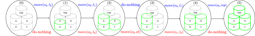
Figure 2: An execution example of a best-effort solution for the arch-building task described in Section 1. Robot actions and human reactions are shown in blue and red, respectively.

4.3 Correctness 

In order to prove Theorem 4.2, we first show the connection between strong and cooperative solutions for the agent goal in a planning domain to winning and cooperatively winning strategies in the corresponding DFA games, respectively.

Theorem 4.3.

Let $\mathcal{D}$ be a planning domain, $\varphi$ an ltl_f goal, and $\mathcal{T}=\mathcal{D}_{+}\circ\mathcal{T}_{\varphi}$ the constructed game arena. The following two hold:

1. there is a strong solution for $\varphi$ in $\mathcal{D}$ iff the agent has a winning strategy in $(\mathcal{T},\mathtt{SafeReach}(\lnot S^{ag}_{err},\,S^{env}_{err}\cup R^{\prime}_{\varphi}))$.

2. there is a cooperative solution for $\varphi$ in $\mathcal{D}$ iff the agent has a cooperatively winning strategy in $(\mathcal{T},\mathtt{SafeReach}(\lnot S^{ag}_{err}\cap\lnot S^{env}_{err},R^{\prime}_{\varphi}))$.

To prove Theorem 4.3, we first observe that a strong solution for $\varphi$ in $\mathcal{D}$ guarantees that the agent always follows its action precondition (i.e., never visits $S^{ag}_{err}$) and either forces the environment to violate its reaction precondition or eventually satisfies $\varphi$ (i.e., eventually reaches $S^{env}_{err}\cup R^{\prime}_{\varphi}$ ). Hence, the agent’s goal is to satisfy

$\Box(\lnot S^{ag}_{err})\land\Diamond(S^{env}_{err}\lor R^{\prime}_{\varphi})$

(For simplicity, we abuse notations and consider sets of states as atomic propositions). Therefore, the reduced game for computing a strong solution is $(\mathcal{T},\mathtt{SafeReach}(\lnot S^{ag}_{err},\,S^{env}_{err}\cup R^{\prime}_{\varphi}))$. Similarly for proving (b).

Next, we show that the safety-reachability games can be solved by reducing to pure reachability games, the correctness of which can be shown by construction.

Lemma 4.4.

Let $\mathcal{T}$, $S^{ag}_{err}$, $S^{env}_{err}$ and $R^{\prime}_{\varphi}$ be as defined above. Then, for every run $\rho$ on $\mathcal{T}$:

• $\rho$ is an accepting run of $\mathtt{SafeReach}(\lnot S^{ag}_{err},\,S^{env}_{err}\cup R^{\prime}_{\varphi})$ iff $\rho$ is an accepting run of $\mathtt{Reach}(\lnot S^{ag}_{err}\cap(S^{env}_{err}\cup R^{\prime}_{\varphi}))$.

• $\rho$ is an accepting run of $\mathtt{SafeReach}(\lnot S^{ag}_{err}\cap\neg S^{env}_{err},R^{\prime}_{\varphi})$ iff $\rho$ is an accepting run of $\mathtt{Reach}(\lnot S^{ag}_{err}\cap S^{env}_{err}\cap R^{\prime}_{\varphi})$.

By Theorem 4.3 and Lemma 4.4, the computed winning strategy $\kappa_{adv}$ for $\mathtt{Reach}(\lnot S^{ag}_{err}\cap(S^{env}_{err}\cup R^{\prime}_{\varphi}))$ and the cooperative winning strategy $\kappa_{coop}$ for $\mathtt{Reach}(\lnot S^{ag}_{err}\cap S^{env}_{err}\cap R^{\prime}_{\varphi})$ indeed correspond to a strong solution and a cooperative solution for $\varphi$ in $\mathcal{D}$, respectively.

We now show that the computed final strategy $\sigma$ by combing $\kappa_{adv}$ and $\kappa_{coop}$ is a best-effort solution for $\varphi$ in $\mathcal{D}$. We prove this through Theorem 3.6 by showing that $\sigma$ satisfies the Maximality Condition.

Theorem 4.5.

Let $\sigma$ be the strategy returned by Algorithm 1. For every $h\in\mathcal{H}_{\mathcal{D}}(\sigma)$ it holds $val(\sigma,h)=val(h)$.

To prove Theorem 4.5, first observe that every sequence of states $\rho$ on $\mathcal{T}$ that does not end at an environment/agent error state corresponds to a legal history $h$ on $\mathcal{D}$. The strategy $\sigma$ returned by Algorithm 1 satisfies that, for every $h\in\mathcal{H}_{\mathcal{D}}(\sigma)$, one of the following holds: (i) the corresponding run $\rho$ on $\mathcal{T}$ ends at a state $s\in W_{adv}$ hence $h$ can surely be extended to satisfy $\varphi$ in $\mathcal{D}$ using $\sigma$ (i.e., from $h$ the agent has a strong solution); (ii) the corresponding run $\rho$ on $\mathcal{T}$ ends at a state $s\in W_{coop}\backslash W_{adv}$ hence $h$ can possibly be extended to satisfy $\varphi$ in $\mathcal{D}$ using $\sigma$, should the environment cooperate (i.e., from $h$ the agent has a cooperative solution); (iii) the corresponding run $\rho$ on $\mathcal{T}$ ends at a state $s\notin W_{coop}\cup W_{adv}$ hence $h$ cannot be extended to satisfy $\varphi$ in $\mathcal{D}$ (i.e., from $h$ the agent has neither a strong nor a cooperative solution). Moreover, $\sigma$ is guaranteed to be a legal strategy since the agent can only perform legal actions.

Finally, we can prove Theorem 4.2 (the correctness of Algorithm 1 in Section 4.2) as an immediate result of Theorems 4.5 and 3.6.

4.4 Computational Complexity 

The computational complexity of ltl_f best-effort synthesis in nondeterministic planning domains is the following:

Theorem 4.6.

ltl_f best-effort synthesis in nondeterministic planning domains is:

• 2EXPTIME-complete in the size of the ltl_f goal;

• EXPTIME-complete in the size of the domain.

Regarding the complexity in the size of the ltl_f goal, the hardness comes from ltl_f synthesis, and the membership comes from the ltl_f-to-DFA construction (double-exponential in the size of the ltl_f formula). Hence, if we consider simple reachability goals in the form of $\varphi=\Diamond(R)$, where $R$ is a propositional formula over the fluents $\mathcal{F}$ of the planning domain, the problem is just polynomial in the size of $\varphi=\Diamond(R)$ since the DFA can be constructed in polynomial time. Regarding the complexity in the size of the domain, the hardness comes from planning itself [18], and the membership comes from the construction of the deterministic transition system from the planning domain (single-exponential in the number of fluents).

An interesting observation from Theorem 4.6 is that best-effort synthesis provides an efficient alternative approach to planning in nondeterministic domains for both ltl_f and reachability goals. In fact, instead of looking for a strong solution, which may not exist, one can look for a best-effort solution, which, on the one hand, always exists and on the other hand is directly a strong solution if the problem admits one.

Running Example (cont.).  We present the computed best-effort solution produced by our synthesis algorithm for the running example in Section 1. We represent the arch-building task as a suitable ltl_f formula and the dynamics of the interactions between the robot and the human (seen as the agent and the environment, respectively) as a nondeterministic planning domain. Figure 2 presents a (simplified) execution example of a best-effort solution to building the arch. Note that at the initial state, all blocks are placed in storage (state $0$). Then the robot successfully placed the block $o_{4}$ at the location $l_{2}$ without any interference from the human (state $1$). Next, the robot placed the block $o_{3}$ at $l_{1}$, and the human helped build the arch by placing $o_{2}$ at $l_{4}$ (state $2$). Seeing the human being cooperative, the robot decides to be lazy, hence not doing anything. However, the human now punishes the robot for being lazy by undoing what the robot has done, thus removing $o_{3}$ back to storage (state $3$). The robot now realizes that the human is not always cooperative, so it proceeds by placing $o_{3}$ back at $l_{1}$, and the human cooperates by placing $o_{1}$ at $l_{3}$ (state $4$). Finally, the robot can build the arch by placing $o_{0}$ at the top, with no interference from the human (state $5$). This example well illustrates the basic characteristic of best-effort solutions: handling both adversarial and cooperative environment behaviors, even if the environment switches back and forth between behaving adversarially and cooperatively instead of always being adversarial or cooperative.

5 Implementation and Empirical Evaluation

We implemented our algorithm for ltl_f best-effort synthesis in planning domains in a tool called BeSyftP, leveraging the symbolic ltl_f synthesis framework [32] that is integrated in all state-of-the-art ltl_f synthesis tools [7, 15]. The explicit-state DFAs of ltl_f formulas are constructed by lydia [16], the overall best-performing tool for ltl_f-to-DFA construction. BeSyftP uses the symbolic DFA encoding proposed in [32] to represent the DFAs symbolically and integrates the symbolic encoding of a planning domain (specified in a variant of PDDL) proposed in [26] for symbolic domain representation. Both symbolic DFAs and planning domains are represented in Binary Decision Diagrams (BDDs) [8], with the BDD library CUDD-3.0.0 [29]. Following [32], BeSyftP constructs and solves symbolic DFA games using Boolean operations provided by CUDD, such as quantification, negation and conjunction. In particular, positional strategies are obtained with Boolean synthesis [22]. Finally, best-effort strategies are computed by applying suitable Boolean operations to the obtained positional winning strategy and cooperatively winning strategy.

Experimental Comparison. To show the efficiency of our technique for ltl_f best-effort synthesis in nondeterministic planning domains, we want to compare it with the approach of reducing to ltl_f best-effort synthesis, by re-expressing the domain as an ltl_f formula. More specifically, we adapted the domain-to-ltl_f translation in [26] to obtain the ltl_f formula $\mathcal{E}$ of the nondeterministic planning domain. Next, we can utilize the ltl_f best-effort synthesis technique from [5] to solve the problem of $\varphi$ (agent goal) under $\mathcal{E}$.

We also evaluated the performance of BeSyftP considering the overhead of computing best-effort solutions wrt computing strong and cooperative solutions. Therefore, we also implemented the adversarial and cooperative synthesis approaches for computing strong and cooperative solutions in AdvSyftP and CoopSyftP, respectively.

Benchmarks. For benchmarks, we consider nondeterministic planning domains as the same one in the running example of building-an-arch described in Section 1. In order to have scalable benchmarks, we consider agent goals as putting $O$ objects at $L$ locations in line, hence the difficulty of the benchmarks increases as either $O$ or $L$ increases. Note that for all these benchmarks, the agent does not have a strong solution to fulfill the goal, i.e., it needs a best-effort solution. Our benchmarks consider at most 8 objects ($1\leq|O|\leq 8$) and 1000 locations ($1\leq|L|\leq 1000$).

Experiment Setup. All experiments were run on a laptop with an operating system 64-bit Ubuntu 20.04, 3.6 GHz CPU, and 12 GB of memory. Time out was set to 1200 seconds.

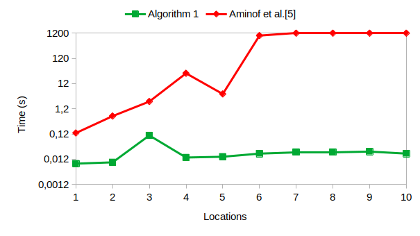
Figure 3: Comparison of BeSyftP and the algorithm from Aminof et al. [5] on benchmarks with $|O|=1$ and $1\leq|L|\leq 10$ (in log scale).

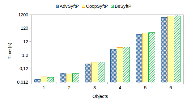
Figure 4: Comparison of BeSyftP, AdvSyftP and CoopSyftP on benchmarks with $|L|=10$ and $1\leq|O|\leq 6$ (in log scale).

Experimental Results. As shown in Figure 3 (for better vision, we only plot the results on instances with up to $10$ locations), utilizing the ltl_f best-effort synthesis approach from [5] can solve the instances with one object ($|O|=1$) up to $6$ locations ($|L|\leq 6$). Instead, BeSyftP can solve all the instances with $|O|=1$ up to $10$ locations and more (up to $1000$), showing much greater scalability.

Figure 4 shows the results of comparing the performance of computing best-effort solutions (BeSyftP) with that of computing strong (AdvSyftP) and cooperative (CoopSyftP) ones. Note that, since all benchmarks are unrealizable, AdvSyftP terminates earlier than both CoopSyftP and BeSyftP (with $20\%\sim 25\%$ less time cost). Interestingly, BeSyftP takes roughly the same time as CoopSyftP (with $10\%\sim 15\%$ more time cost). This shows that, although computing a best-effort solution requires solving two games and combining the computed adversarial and cooperative solutions, BeSyftP requires only a small overhead with respect to both AdvSyftP and CoopSyftP.

6 Conclusion

In this paper, we have developed a framework for ltl_f best-effort synthesis in nondeterministic (adversarial) planning domains, and a solution technique that admits a scalable symbolic implementation. The approach presented here can be extended to different forms of goal specification. In particular, we can expect a further complexity reduction if we express goals in pure-past temporal logics [14]. Also, the game-based techniques adopted here could possibly be extended to handle best-effort synthesis under multiple environment specifications [13, 1, 2]. Another promising extension is considering maximally permissive strategies [30], which allows the agent to choose a best-effort solution during execution instead of committing to a single solution beforehand We leave this for future work.

References

- [1] Benjamin Aminof, Giuseppe De Giacomo, Alessio Lomuscio, Aniello Murano, and Sasha Rubin, ‘Synthesizing strategies under expected and exceptional environment behaviors’, in IJCAI, pp. 1674–1680, (2020).
- [2] Benjamin Aminof, Giuseppe De Giacomo, Alessio Lomuscio, Aniello Murano, and Sasha Rubin, ‘Synthesizing best-effort strategies under multiple environment specifications’, in KR, pp. 42–51, (2021).
- [3] Benjamin Aminof, Giuseppe De Giacomo, Aniello Murano, and Sasha Rubin, ‘Planning and synthesis under assumptions’, arXiv, (2018).
- [4] Benjamin Aminof, Giuseppe De Giacomo, Aniello Murano, and Sasha Rubin, ‘Planning under LTL environment specifications’, in ICAPS, pp. 31–39, (2019).
- [5] Benjamin Aminof, Giuseppe De Giacomo, and Sasha Rubin, ‘Best-Effort Synthesis: Doing Your Best Is Not Harder Than Giving Up’, in IJCAI, pp. 1766–1772, (2021).
- [6] Christel Baier, Joost-Pieter Katoen, and Kim Guldstrand Larsen, Principles of Model Checking, MIT Press, 2008.
- [7] Suguman Bansal, Yong Li, Lucas M. Tabajara, and Moshe Y. Vardi, ‘Hybrid compositional reasoning for reactive synthesis from finite-horizon specifications’, in AAAI, pp. 9766–9774, (2020).
- [8] Randal E. Bryant, ‘Symbolic Boolean Manipulation with Ordered Binary-Decision Diagrams’, ACM Comput. Surv., 24(3), 293–318, (1992).
- [9] Alberto Camacho, Meghyn Bienvenu, and Sheila A McIlraith, ‘Towards a unified view of ai planning and reactive synthesis’, in ICAPS, pp. 58–67, (2019).
- [10] Alberto Camacho and Sheila A. McIlraith, ‘Strong fully observable non-deterministic planning with LTL and LTLf goals’, in IJCAI, pp. 5523–5531, (2019).
- [11] Alessandro Cimatti, Marco Pistore, Marco Roveri, and Paolo Traverso, ‘Weak, strong, and strong cyclic planning via symbolic model checking.’, AIJ, 1–2(147), 35–84, (2003).
- [12] Alessandro Cimatti, Marco Roveri, and Paolo Traverso, ‘Strong planning in non-deterministic domains via model checking’, in AIPS, pp. 36–43, (1998).
- [13] Daniel Alfredo Ciolek, Nicolás D’Ippolito, Alberto Pozanco, and Sebastian Sardiña, ‘Multi-tier automated planning for adaptive behavior’, in ICAPS, pp. 66–74, (2020).
- [14] Giuseppe De Giacomo, Antonio Di Stasio, Francesco Fuggitti, and Sasha Rubin, ‘Pure-past linear temporal and dynamic logic on finite traces’, in IJCAI, pp. 4959–4965, (2020).
- [15] Giuseppe De Giacomo and Marco Favorito, ‘Compositional approach to translate LTLf/LDLf into deterministic finite automata’, in ICAPS, pp. 122–130, (2021).
- [16] Giuseppe De Giacomo and Marco Favorito, ‘Lydia: A tool for compositional LTLf /LDLf synthesis’, in ICAPS, pp. 122–130, (2021).
- [17] Giuseppe De Giacomo and Yves Lespérance, ‘The nondeterministic situation calculus’, in KR, pp. 216–226, (2021).
- [18] Giuseppe De Giacomo and Sasha Rubin, ‘Automata-Theoretic Foundations of FOND Planning for LTLf and LDLf Goals.’, in IJCAI, pp. 4729–4735, (2018).
- [19] Giuseppe De Giacomo and Moshe Y. Vardi, ‘Linear Temporal Logic and Linear Dynamic Logic on Finite Traces’, in IJCAI, pp. 854–860, (2013).
- [20] Giuseppe De Giacomo and Moshe Y. Vardi, ‘Synthesis for LTL and LDL on Finite Traces’, in IJCAI, pp. 1558–1564, (2015).
- [21] Bernd Finkbeiner, ‘Synthesis of Reactive Systems.’, Dependable Software Systems Eng., 45, 72–98, (2016).
- [22] Dror Fried, Lucas M. Tabajara, and Moshe Y. Vardi, ‘BDD-based Boolean functional synthesis’, in CAV, pp. 402–421, (2016).
- [23] H. Geffner and B. Bonet, A Concise Introduction to Models and Methods for Automated Planning, 2013.
- [24] Malik Ghallab, Dana S. Nau, and Paolo Traverso, Automated planning - theory and practice, 2004.
- [25] Patrik Haslum, Nir Lipovetzky, Daniele Magazzeni, and Christian Muise, An Introduction to the Planning Domain Definition Language, 2019.
- [26] Keliang He, Andrew M Wells, Lydia E Kavraki, and Moshe Y Vardi, ‘Efficient Symbolic Reactive Synthesis for Finite-Horizon Tasks’, in ICRA, pp. 8993–8999, (2019).
- [27] A. Pnueli and R. Rosner, ‘On the synthesis of a reactive module’, in POPL, p. 179–190, (1989).
- [28] Amir Pnueli, ‘The temporal logic of programs’, in FOCS, pp. 46–57, (1977).
- [29] Fabio Somenzi, ‘CUDD: CU Decision Diagram Package 3.0.0. Universiy of Colorado at Boulder’, (2016).
- [30] Shufang Zhu and Giuseppe De Giacomo, ‘Synthesis of maximally permissive strategies for ltlf specifications’, in IJCAI, pp. 2783–2789. ijcai.org, (2022).
- [31] Shufang Zhu, Lucas M. Tabajara, Jianwen Li, Geguang Pu, and Moshe Y. Vardi, ‘A symbolic approach to safety LTL synthesis’, in HVC, pp. 147–162, (2017).
- [32] Shufang Zhu, Lucas M. Tabajara, Jianwen Li, Geguang Pu, and Moshe Y. Vardi, ‘Symbolic LTLf Synthesis’, in IJCAI, pp. 1362–1369, (2017).
- [33] Martin Zimmermann, Felix Klein, and Alexander Weinert, ‘Infinite games’, in Lecture Notes (Chapters 1 and 2), (2016).