Stabilised finite element method for Stokes problem with nonlinear slip condition

Abstract

This work introduces a stabilised finite element formulation for the Stokes flow problem with a nonlinear slip boundary condition of friction type. The boundary condition is enforced with the help of an additional Lagrange multiplier and the stabilised formulation is based on simultaneously stabilising both the pressure and the Lagrange multiplier. We establish the stability and the a priori error analyses, and perform a numerical convergence study in order to verify the theory.

1 Introduction

The Stokes problem is a well known and extensively studied linear model for creeping flow. There exist various physically justified and mathematically valid boundary conditions that can be directly applied. For instance, some components of the velocity field $\boldsymbol{u}$ may be prescribed while the other components are free to vary subject to a zero shear stress condition. In the classical slip boundary condition, the normal velocity is equal to zero and the tangential velocity remains unspecified. This could represent, for instance, the free interface between a glacier and the atmosphere where the shear stress is negligible [21, 10].

However, in some cases a more involved nonlinear interaction takes place between the fluid and its surroundings. Think, e.g., of a membrane leaking only if the pressure becomes large enough. Another example is a slip flow in which the tangential velocity at the boundary becomes nonzero if and only if the shear stress exceeds a prescribed, or velocity-dependent, friction threshold. This inequality-type of friction laws have been suggested, e.g., for the flow of glaciers over the bedrock [24]. Besides, given that the Stokes flow problem is analogous to the equations of linear elasticity in the incompressible limit [17], nonlinear slip conditions could be used for modeling frictional contact of incompressible solids.

In this work, we focus on the nonlinear slip condition with a prescribed friction threshold. The nonlinear slip (and leak) boundary conditions of friction type were first considered for incompressible fluids by Fujita [9]—see also the discussion on slip boundary conditions for fluid flow problems in Le Roux [18]. These problems can be written as variational inequalities of the second kind, cf. Fujita [9], or, alternatively, as mixed variational inequalities by expressing the boundary traction as a Lagrange multiplier $\boldsymbol{\lambda}$ which enforces the inequality constraint, cf. [3]. Here, we adopt the second formulation and propose a stabilized finite element method for its numerical approximation.

Regarding the numerical approximations, Kashiwabara [16] has proven error estimates for the velocity-pressure pair $(\boldsymbol{u},p)$ using Taylor–Hood $P_{2}$–$P_{1}$ finite elements but with the inf-sup constant for the tangential component $\boldsymbol{\lambda}_{t}$, approximated using the trace space of $P_{2}$, still depending on $h$. The lack of uniform stability means that it is not possible to achieve optimal error estimates for $\boldsymbol{\lambda}_{t}$. However, the value of $\boldsymbol{\lambda}_{t}$ is needed in finding the active constraints at each iteration step of the solution algorithm. Therefore, it is reasonable to aim at uniform stability for the three unknowns $(\boldsymbol{u},p,\boldsymbol{\lambda})$.

Achieving uniform stability simultaneously for $\boldsymbol{\lambda}$ and $p$ can be done by different means, e.g., by a specific choice of finite element spaces. The work of Ayadi et al. [3, 2, 1] is based on the use of $P_{1}$ bubble–$P_{1}$–$P_{1}$ triplet as a stable choice of mixed finite element spaces. This is a reasonable choice since $P_{1}$ bubble–$P_{1}$ for $(\boldsymbol{u},p)$ is known to be stable in the case of the standard Stokes problem and $P_{1}$–$P_{1}$ element for $(\boldsymbol{u},\boldsymbol{\lambda})$ has been implemented to impose boundary conditions using Lagrange multipliers—although we would expect that minor modifications of the basis functions are needed in the case of mixed boundary conditions [13]. Other works based on mixed methods, with or without an explicit Lagrange multiplier for the boundary condition, include Djoko et al. [5, 7] and Fang et al. [8].

The present work focuses on Barbosa–Hughes stabilisation [4], i.e. the inclusion of additional residual terms in the variational formulation to circumvent the Babuška–Brezzi condition. If these residual terms are consistent and scaled properly, it is possible to have stability for the $(p,\boldsymbol{\lambda})$ variables, no matter which finite element spaces are considered for discretisation. This will greatly improve the flexibility in choosing the finite element spaces and allows for discretisations beyond those based on the boundary conditions. In this work, the stabilisation allows us to use the lowest order $P_{1}$–$P_{1}$–$P_{0}$ element in our numerical experiment, a triplet which would otherwise be unstable.

Residual stabilisation has been considered in Djoko–Koko [6] but only for the velocity–pressure pair and, hence, without estimates for $\boldsymbol{\lambda}$. A stabilisation technique through pressure projection has been presented in Li–Li [20], and discussed in Qiu et al. [22] and Li et al. [19], but again without estimates for $\boldsymbol{\lambda}$. Using residual stabilisation for both Lagrange multipliers, $p$ and $\boldsymbol{\lambda}$, we establish here a uniform stability estimate for all three variables. This is shown to lead to a quasi-optimality result which is further refined into an a priori error estimate for the lowest order method.

The work is organized as follows. In Section 2, we present the strong formulation of the problem and in Section 3 derive the corresponding weak formulation. The stabilised finite element method is presented and its stability analysed in Section 4. In Section 5, the quasi-optimality estimate is proven and shown to provide an optimal priori error estimate for the lowest order method. In Section 6, we derive a solution algorithm for the discrete variational inequality and, in Section 7, report on the results of our numerical experiment which aims at corroborating the theoretical convergence rates.

2 Strong formulation

Let $\Omega\in\mathbb{R}^{d},d\in\{2,3\}$ denote a polygonal (polyhedral) domain with a Lipschitz boundary $\partial\Omega$ and let $\boldsymbol{u}:\Omega\rightarrow\mathbb{R}^{d}$ be the fluid velocity field. Denoting the symmetric part of the velocity gradient by

$$\boldsymbol{D}(\boldsymbol{u})=\frac{1}{2}(\nabla\boldsymbol{u}+\nabla\boldsymbol{u}^{T}),$$

we introduce the differential operator

$$\boldsymbol{A}\boldsymbol{u}=\boldsymbol{u}-\,\mathbf{div}\,(2\mu\boldsymbol{D}(\boldsymbol{u})),$$

where $\mu>0$ is the kinematic viscosity. Letting $p:\Omega\rightarrow\mathbb{R}$ be the pressure field, the balance of linear momentum for an incompressible, homogeneous and linearly viscous fluid reads as

(1) $$\boldsymbol{A}\boldsymbol{u}+\nabla p=\boldsymbol{f},$$

where $\boldsymbol{f}:\Omega\rightarrow\mathbb{R}^{d}$ denotes the resultant of external forces and which holds together with the incompressibility constraint

(2) $$\mathrm{div}\,\boldsymbol{u}=0.$$

Remark 1.

We are considering here the ”generalized” Stokes system (1)–(2) for expediency. In particular, using the operator $\boldsymbol{A}\boldsymbol{u}$, instead of $-\,\mathbf{div}\,(2\mu\boldsymbol{D}(\boldsymbol{u}))$, allows us to impose the slip boundary condition on the entire $\partial\Omega$. Considering different boundary conditions at different parts of the domain requires resorting to the trace space $H^{1/2}_{00}$ [25] for the normal components of the velocity field trace which, in our opinion, is an unnecessary technical difficulty. We also note that the generalized equation is relevant, as such, for the implicit time discretization of the time-dependent Stokes equations, and that the solvers presented in this work and available at [11] can be applied to the standard Stokes system by simply removing the additional term.

Next, let us introduce the boundary conditions. Denoting the Cauchy stress tensor by

(3) $$\boldsymbol{\sigma}(\boldsymbol{u},p)=-p\boldsymbol{I}+2\mu\boldsymbol{D}(\boldsymbol{u}),$$

and the normal and tangential components of $\boldsymbol{u}$ as $u_{n}=\boldsymbol{u}\cdot\boldsymbol{n}$ and $\boldsymbol{u}_{t}=\boldsymbol{u}-u_{n}\boldsymbol{n}$, where $\boldsymbol{n}:\partial\Omega\rightarrow\mathbb{R}^{d}$ is the outward unit normal to $\Omega$, we divide the normal stress vector $\boldsymbol{\sigma}(\boldsymbol{u},p)\boldsymbol{n}$ into its normal and tangential components $\sigma_{n}$ and $\boldsymbol{\sigma}_{t}$ defined through

$$\sigma_{n}(\boldsymbol{u},p)=\boldsymbol{\sigma}(\boldsymbol{u},p)\boldsymbol{n}\cdot\boldsymbol{n}$$

and

$$\boldsymbol{\sigma}_{t}(\boldsymbol{u},p)=\boldsymbol{\sigma}(\boldsymbol{u},p)\boldsymbol{n}-\sigma_{n}(\boldsymbol{u},p)\boldsymbol{n}.$$

On the boundary $\partial\Omega$, we impose the following (nonlinear) slip boundary condition

(4) $$u_{n}=0,\quad|\boldsymbol{\sigma}_{t}|\leq\kappa,\quad\boldsymbol{\sigma}_{t}\cdot\boldsymbol{u}_{t}+\kappa|\boldsymbol{u}_{t}|=0,$$

where $\kappa:\partial\Omega\rightarrow(0,\infty)$ is a positive threshold function denoting an upper limit for the tangential stress before slip occurs. In case the boundary condition is imposed with the help of Lagrange multipliers, the definition

(5) $$\boldsymbol{\lambda}=\boldsymbol{\sigma}(\boldsymbol{u},p)\boldsymbol{n}$$

implies that

(6) $$\lambda_{n}u_{n}=0,\quad|\boldsymbol{\lambda}_{t}|\leq\kappa,\quad\boldsymbol{\lambda}_{t}\cdot\boldsymbol{u}_{t}+\kappa|\boldsymbol{u}_{t}|=0,$$

where $\lambda_{n}=\boldsymbol{\lambda}\cdot\boldsymbol{n}$ denotes the normal component of the Lagrange multiplier and $\boldsymbol{\lambda}_{t}=\boldsymbol{\lambda}-\lambda_{n}\boldsymbol{n}$ its tangential component.

Remark 2.

Note that there exists an analogous interpretation of the above problem in solid mechanics. It is well known that the Stokes problem (1)–(2) can be obtained from the equations of linear elasticity by defining ”pressure” as the product of the first Lamé parameter and the divergence of the displacement field and then letting the first Lamé parameter approach infinity, corresponding to the incompressible limit. Consequently, in solid mechanics, the condition (4) can be referred to as the Tresca friction condition [14].

3 Mixed variational formulation

We will now present a mixed variational formulation for problem (1),(2), (4). We use the following notation for the $L^{2}$ inner products

$$(a,b)=\int_{\Omega}ab\,\mathrm{d}x,\quad(\boldsymbol{a},\boldsymbol{b})=\int_{\Omega}\boldsymbol{a}\cdot\boldsymbol{b}\,\mathrm{d}x,$$

define the velocity and pressure spaces through

$$\boldsymbol{V}=H^{1}(\Omega)^{d},\quad Q=\{q\in L^{2}(\Omega):(q,1)=0\},$$

and denote the trace space by $\boldsymbol{W}=H^{1/2}(\partial\Omega)^{d}$, $d\in\{2,3\}$. The space for the Lagrange multiplier, defined in (5), is

$$\boldsymbol{\varLambda}=\{\boldsymbol{\mu}\in\boldsymbol{M}:\langle\boldsymbol{\mu}_{t},\boldsymbol{v}\rangle\leq(\kappa,|\boldsymbol{v}_{t}|)_{\partial\Omega}~{}\forall\boldsymbol{v}\in\boldsymbol{W}\},$$

where $\boldsymbol{M}=\boldsymbol{W}^{\prime}$ and $\langle.,.\rangle$ denotes the duality pairing between $\boldsymbol{M}$ and $\boldsymbol{W}$. In particular, for $\boldsymbol{\mu}\in\boldsymbol{M}$ and $\boldsymbol{v}=(v_{n}\boldsymbol{n}+\boldsymbol{v}_{t})\in\boldsymbol{W}$ we can write

$$\langle\boldsymbol{\mu},\boldsymbol{v}\rangle=\langle\mu_{n},v_{n}\rangle+\langle\boldsymbol{\mu}_{t},\boldsymbol{v}_{t}\rangle,$$

where $\langle\mu_{n},v_{n}\rangle=\langle\mu_{n}\boldsymbol{n},v_{n}\boldsymbol{n}\rangle$; cf. [28].

The mixed variational formulation of problem (1),(2), (4) now reads as follows: find $(\boldsymbol{u},p,\boldsymbol{\lambda})\in\boldsymbol{V}\times Q\times\boldsymbol{\varLambda}$ such that

(7) $$\left\{\begin{aligned} a(\boldsymbol{u},\boldsymbol{v})-(\mathrm{div}\,\boldsymbol{v},p)-\langle\boldsymbol{\lambda},\boldsymbol{v}\rangle&=(\boldsymbol{f},\boldsymbol{v})\quad&&\forall\boldsymbol{v}\in\boldsymbol{V},\\ (\mathrm{div}\,\boldsymbol{u},q)&=0\quad&&\forall q\in Q,\ \\ -\langle\boldsymbol{\mu}-\boldsymbol{\lambda},\boldsymbol{u}\rangle&\leq 0\quad&&\forall\boldsymbol{\mu}\in\boldsymbol{\varLambda}.\end{aligned}\right.$$

The existence, uniqueness and regularity of solutions of the variational problem (without the Lagrange multiplier) has been studied in [9] and [23].

We can write problem (7) in more compact form by defining the bilinear form

$$\mathcal{B}(\boldsymbol{w},r,\boldsymbol{\xi};\boldsymbol{v},q,\boldsymbol{\mu}) =a(\boldsymbol{w},\boldsymbol{v})-(q,\mathrm{div}\,\boldsymbol{w})-(r,\mathrm{div}\,\boldsymbol{v})-\langle\boldsymbol{\xi},\boldsymbol{v}\rangle-\langle\boldsymbol{\mu},\boldsymbol{w}\rangle$$

where

$$a(\boldsymbol{w},\boldsymbol{v})=(\boldsymbol{w},\boldsymbol{v})+(2\mu\boldsymbol{D}(\boldsymbol{w}),\boldsymbol{D}(\boldsymbol{v})).$$

Problem 1 (Continuous variational form).

Find $(\boldsymbol{u},p,\boldsymbol{\lambda})\in\boldsymbol{V}\times Q\times\boldsymbol{\varLambda}$ such that

$$\mathcal{B}(\boldsymbol{u},p,\boldsymbol{\lambda};\boldsymbol{v},q,\boldsymbol{\mu}-\boldsymbol{\lambda})\leq(\boldsymbol{f},\boldsymbol{v})\quad\forall(\boldsymbol{v},q,\boldsymbol{\mu})\in\boldsymbol{V}\times Q\times\boldsymbol{\varLambda}.$$

The following norm will be used in our analysis:

(8) $${\left|\kern-1.07639pt\left|\kern-1.07639pt\left|(\boldsymbol{w},r,\boldsymbol{\xi})\right|\kern-1.07639pt\right|\kern-1.07639pt\right|}^{2}=\|\boldsymbol{w}\|_{1,\Omega}^{2}+\|r\|_{0,\Omega}^{2}+\|\boldsymbol{\xi}\|_{-\frac{1}{2}}^{2},$$

where $\|\cdot\|_{1,\Omega}$ and $\|\cdot\|_{0,\Omega}$ are the usual norms in the Hilbert spaces $H^{1}(\Omega)$ and $L^{2}(\Omega)$ and

$$\|\boldsymbol{\xi}\|_{-\frac{1}{2}}=\sup_{\boldsymbol{w}\in\boldsymbol{W}}\frac{\langle\boldsymbol{\xi},\boldsymbol{w}\rangle}{\|\boldsymbol{w}\|_{\frac{1}{2}}}\quad\text{and}\quad\|\boldsymbol{w}\|_{\frac{1}{2}}=\inf_{\begin{subarray}{c}\boldsymbol{v}\in(H^{1}(\Omega))^{d}\\ \boldsymbol{v}|_{\partial\Omega}=\boldsymbol{w}\end{subarray}}\|\nabla\boldsymbol{v}\|_{0}.$$

Note that there exist $C,c>0$ such that

(9) $$c\|\boldsymbol{w}\|_{1,\Omega}^{2}\leq a(\boldsymbol{w},\boldsymbol{w})\leq C\|\boldsymbol{w}\|_{1,\Omega}^{2}.$$

In the following, we write $a\lesssim b$ (or $a\gtrsim b$) if there exists a constant $C>0$, which is independent of the finite element mesh, but possibly varying from step to step, and satisfies $a\leq Cb$ (or $a\geq Cb$).

The proof of the following result can be found, e.g., in [2].

Theorem 1 (Continuous stability).

For every $(\boldsymbol{w},r,\boldsymbol{\xi})\in\boldsymbol{V}\times Q\times\boldsymbol{\varLambda}$ there exists $(\boldsymbol{v},q,\boldsymbol{\mu})\in\boldsymbol{V}\times Q\times\boldsymbol{\varLambda}$ satisfying

$$\mathcal{B}(\boldsymbol{w},r,\boldsymbol{\xi};\boldsymbol{v},q,\boldsymbol{\mu})\gtrsim{\left|\kern-1.07639pt\left|\kern-1.07639pt\left|(\boldsymbol{w},r,\boldsymbol{\xi})\right|\kern-1.07639pt\right|\kern-1.07639pt\right|}^{2}$$

and

$${\left|\kern-1.07639pt\left|\kern-1.07639pt\left|(\boldsymbol{v},q,\boldsymbol{\mu})\right|\kern-1.07639pt\right|\kern-1.07639pt\right|}\lesssim{\left|\kern-1.07639pt\left|\kern-1.07639pt\left|(\boldsymbol{w},r,\boldsymbol{\xi})\right|\kern-1.07639pt\right|\kern-1.07639pt\right|}.$$

4 Stabilized finite element method

We consider finite element spaces based on a shape regular triangulation $\mathcal{T}_{h}$ of $\Omega$ with the mesh parameter $h$. We denote by $\mathcal{E}_{h}$ the internal facets and by $\mathcal{G}_{h}$ the boundary facets of $\mathcal{T}_{h}$, respectively. The finite element spaces are denoted by $\boldsymbol{V}_{h}\subset\boldsymbol{V}$, $Q_{h}\subset Q$, $\boldsymbol{M}_{h}\subset\boldsymbol{M}$, and, in addition, we define the discrete counterpart of $\boldsymbol{\varLambda}$ as follows:

$$\boldsymbol{\varLambda}_{h}=\{\boldsymbol{\mu}\in\boldsymbol{M}_{h}:|\boldsymbol{\mu}_{t}|\leq\kappa\}.$$

Our analysis is based on the conformity assumption $\boldsymbol{\varLambda}_{h}\subset\boldsymbol{\varLambda}$ which means that we must be able to enforce the condition $|\boldsymbol{\lambda}_{h,t}|\leq\kappa$ strongly. In practice, this means, e.g., that $\kappa$ and $\boldsymbol{\lambda}_{h}$ are constants elementwise. We note that while the conformity is required by our analysis, the resulting algorithm gives reasonable results also for nonconstant $\kappa$ where the condition $|\boldsymbol{\lambda}_{h,t}|\leq\kappa$ holds only, e.g., at element midpoints or at the nodes of the mesh.

Let $\alpha_{1},\alpha_{2}>0$ be stabilization parameters. The finite element method is written with the help of the stabilized bilinear form

$$\mathcal{B}_{h}(\boldsymbol{w},r,\boldsymbol{\xi};\boldsymbol{v},q,\boldsymbol{\mu})=\mathcal{B}(\boldsymbol{w},r,\boldsymbol{\xi};\boldsymbol{v},q,\boldsymbol{\mu})-\alpha_{1}\mathcal{S}_{h}^{1}(\boldsymbol{w},r;\boldsymbol{v},q)-\alpha_{2}\mathcal{S}_{h}^{2}(\boldsymbol{w},r,\boldsymbol{\xi};\boldsymbol{v},q,\boldsymbol{\mu})$$

where

$$\mathcal{S}_{h}^{1}(\boldsymbol{w},r;\boldsymbol{v},q)=\sum_{T\in\mathcal{T}_{h}}h_{T}^{2}\int_{T}(\boldsymbol{A}\boldsymbol{w}+\nabla r)\cdot(\boldsymbol{A}\boldsymbol{v}+\nabla q)\,\mathrm{d}x$$

and

$$\mathcal{S}_{h}^{2}(\boldsymbol{w},r,\boldsymbol{\xi};\boldsymbol{v},q,\boldsymbol{\mu})=\sum_{E\in\mathcal{G}_{h}}h_{E}\int_{E}(\boldsymbol{\xi}-\boldsymbol{\sigma}(\boldsymbol{w},r)\boldsymbol{n})\cdot(\boldsymbol{\mu}-\boldsymbol{\sigma}(\boldsymbol{v},q)\boldsymbol{n})\,\mathrm{d}s.$$

The stabilized linear form is given by

$$\mathcal{L}_{h}(\boldsymbol{v},q)=(\boldsymbol{f},\boldsymbol{v})-\alpha_{1}\mathcal{F}_{h}(\boldsymbol{v},q)$$

where

$$\mathcal{F}_{h}(\boldsymbol{v},q)=\sum_{T\in\mathcal{T}_{h}}h_{T}\int_{T}\boldsymbol{f}\cdot(\boldsymbol{A}\boldsymbol{v}+\nabla q)\,\mathrm{d}x.$$

The stabilized finite element method corresponds to solving the following variational problem.

Problem 2 (Discrete variational form).

Find $(\boldsymbol{u}_{h},p_{h},\boldsymbol{\lambda}_{h})\in\boldsymbol{V}_{h}\times Q_{h}\times\boldsymbol{\varLambda}_{h}$ such that

$$\mathcal{B}_{h}(\boldsymbol{u}_{h},p_{h},\boldsymbol{\lambda}_{h};\boldsymbol{v}_{h},q_{h},\boldsymbol{\mu}_{h}-\boldsymbol{\lambda}_{h})\leq\mathcal{L}_{h}(\boldsymbol{v}_{h},q_{h})\quad\forall(\boldsymbol{v}_{h},q_{h},\boldsymbol{\mu}_{h})\in\boldsymbol{V}_{h}\times Q_{h}\times\boldsymbol{\varLambda}_{h}.$$

In our analysis, we will use the following inverse and trace estimates, easily proven by a scaling argument.

Lemma 1 (Inverse estimates).

For any $(\boldsymbol{w}_{h},r_{h})\in\boldsymbol{V}_{h}\times Q_{h}$, there exist constants $C_{I,1},C_{I,2}>0$ such that

$$C_{I,1}\sum_{T\in\mathcal{T}_{h}}h_{T}^{2}\|\boldsymbol{A}\boldsymbol{w}_{h}\|_{0,T}^{2}\leq a(\boldsymbol{w}_{h},\boldsymbol{w}_{h})$$

and

$$C_{I,2}\sum_{E\in\mathcal{G}_{h}}h_{E}\|\boldsymbol{\sigma}(\boldsymbol{w}_{h},r_{h})\boldsymbol{n}\|_{0,E}^{2}\leq a(\boldsymbol{w}_{h},\boldsymbol{w}_{h}).$$

Lemma 2 (Discrete trace estimate).

For any $\boldsymbol{w}_{h}\in\boldsymbol{V}_{h}$, there exists $C_{T}>0$ such that

$$C_{T}\sum_{E\in\mathcal{G}_{h}}h_{E}\|2\mu\boldsymbol{D}(\boldsymbol{w}_{h})\boldsymbol{n}\|_{0,E}^{2}\leq\|\boldsymbol{w}_{h}\|_{1,\Omega}^{2}.$$

The following discrete counterpart of the norm defined in (8) is instrumental in the stability analysis of the discrete problem.

(10) $${\left|\kern-1.07639pt\left|\kern-1.07639pt\left|(\boldsymbol{w}_{h},r_{h},\boldsymbol{\xi}_{h})\right|\kern-1.07639pt\right|\kern-1.07639pt\right|}^{2}_{h}={\left|\kern-1.07639pt\left|\kern-1.07639pt\left|(\boldsymbol{w}_{h},r_{h},\boldsymbol{\xi}_{h})\right|\kern-1.07639pt\right|\kern-1.07639pt\right|}^{2}+\sum_{T\in\mathcal{T}_{h}}h_{T}^{2}\|\nabla r_{h}\|_{0,T}^{2}+\sum_{E\in\mathcal{G}_{h}}h_{E}\|\boldsymbol{\xi}_{h}\|^{2}_{0,E}.$$

Note, in particular, that

(11) $${\left|\kern-1.07639pt\left|\kern-1.07639pt\left|(\boldsymbol{w}_{h},r_{h},\boldsymbol{\xi}_{h})\right|\kern-1.07639pt\right|\kern-1.07639pt\right|}_{h}\geq{\left|\kern-1.07639pt\left|\kern-1.07639pt\left|(\boldsymbol{w}_{h},r_{h},\boldsymbol{\xi}_{h})\right|\kern-1.07639pt\right|\kern-1.07639pt\right|}.$$

Existence and uniqueness of solutions to the discrete variational problem follows from the discrete stability estimate proven below.

Theorem 2 (Discrete stability).

Let $\frac{\alpha_{1}}{C_{I,1}}+\frac{\alpha_{2}}{C_{I,2}}<1$. For every $(\boldsymbol{w}_{h},r_{h},\boldsymbol{\xi}_{h})\in\boldsymbol{V}_{h}\times Q_{h}\times\boldsymbol{\varLambda}_{h}$ there exists $(\boldsymbol{v}_{h},q_{h})\in\boldsymbol{V}_{h}\times Q_{h}$ satisfying

(12) $$\mathcal{B}_{h}(\boldsymbol{w}_{h},r_{h},\boldsymbol{\xi}_{h};\boldsymbol{v}_{h},q_{h},-\boldsymbol{\xi}_{h})\gtrsim{\left|\kern-1.07639pt\left|\kern-1.07639pt\left|(\boldsymbol{w}_{h},r_{h},\boldsymbol{\xi}_{h})\right|\kern-1.07639pt\right|\kern-1.07639pt\right|}_{h}^{2}$$

and

$${\left|\kern-1.07639pt\left|\kern-1.07639pt\left|(\boldsymbol{v}_{h},q_{h},\boldsymbol{\mu}_{h})\right|\kern-1.07639pt\right|\kern-1.07639pt\right|}_{h}\lesssim{\left|\kern-1.07639pt\left|\kern-1.07639pt\left|(\boldsymbol{w}_{h},r_{h},\boldsymbol{\mu}_{h})\right|\kern-1.07639pt\right|\kern-1.07639pt\right|}_{h}\quad\forall\boldsymbol{\mu}_{h}\in\boldsymbol{\varLambda}_{h}.$$

Proof.

(Step 1.) Choosing $(\boldsymbol{v}_{h},q_{h},\boldsymbol{\mu}_{h})=(\boldsymbol{w}_{h},-r_{h},-\boldsymbol{\xi}_{h})$ gives

$$\mathcal{B}_{h}(\boldsymbol{w}_{h},r_{h},\boldsymbol{\xi}_{h};\boldsymbol{w}_{h},-r_{h},-\boldsymbol{\xi}_{h})$$

$$=a(\boldsymbol{w}_{h},\boldsymbol{w}_{h})-\alpha_{1}\sum_{T\in\mathcal{T}_{h}}h_{T}^{2}\|\boldsymbol{A}\boldsymbol{w}_{h}\|_{0,T}^{2}-\alpha_{2}\sum_{E\in\mathcal{G}_{h}}h_{E}\|\boldsymbol{\sigma}(\boldsymbol{w}_{h},r_{h})\boldsymbol{n}\|_{0,E}^{2}$$

$$\quad+\alpha_{1}\sum_{T\in\mathcal{T}_{h}}h_{T}^{2}\|\nabla r_{h}\|_{0,T}^{2}+\alpha_{2}\sum_{E\in\mathcal{G}_{h}}h_{E}\|\boldsymbol{\xi}_{h}\|^{2}_{0,E}.$$

Using the inverse estimates of Lemma 1 and the bound (9) we get

$$\mathcal{B}_{h}(\boldsymbol{w}_{h},r_{h},\boldsymbol{\xi}_{h};\boldsymbol{w}_{h},-r_{h},-\boldsymbol{\xi}_{h})$$

$$\geq\left(1-\frac{\alpha_{1}}{C_{I,1}}-\frac{\alpha_{2}}{C_{I,2}}\right)c\|\boldsymbol{w}_{h}\|_{1,\Omega}^{2}+\alpha_{1}\sum_{T\in\mathcal{T}_{h}}h_{T}^{2}\|\nabla r_{h}\|_{0,T}^{2}+\alpha_{2}\sum_{E\in\mathcal{G}_{h}}h_{E}\|\boldsymbol{\xi}_{h}\|^{2}_{0,E}.$$

(Step 2.) As a consequence of Theorem 1, for any $(r_{h},\boldsymbol{\xi}_{h})\in Q_{h}\times\boldsymbol{\varLambda}_{h}$ there exists $\boldsymbol{v}\in\boldsymbol{V}$ such that

(13) $$(r_{h},\mathrm{div}\,\boldsymbol{v})+\langle\boldsymbol{\xi}_{h},\boldsymbol{v}\rangle\geq C_{1}(\|r_{h}\|_{0,\Omega}^{2}+\|\boldsymbol{\xi}_{h}\|_{-\frac{1}{2}}^{2})$$

and

(14) $$\|\boldsymbol{v}\|_{1,\Omega}^{2}\leq C_{2}(\|r_{h}\|_{0,\Omega}^{2}+\|\boldsymbol{\xi}_{h}\|_{-\frac{1}{2}}^{2})$$

where $C_{1},C_{2}>0$. Let $\widetilde{\boldsymbol{v}}\in\boldsymbol{V}_{h}$ be the Clemént interpolant of $\boldsymbol{v}$ with the properties

(15) $$\left(\sum_{T\in\mathcal{T}_{h}}h_{T}^{-2}\|\boldsymbol{v}-\widetilde{\boldsymbol{v}}\|_{0,T}^{2}\right)^{1/2}+\left(\sum_{E\in\mathcal{G}_{h}}h_{E}^{-1}\|\boldsymbol{v}-\widetilde{\boldsymbol{v}}\|_{0,E}^{2}\right)^{1/2}\leq C_{i,1}\|\boldsymbol{v}\|_{1,\Omega}$$

and

(16) $$\|\widetilde{\boldsymbol{v}}\|_{1,\Omega}\leq C_{i,2}\|\boldsymbol{v}\|_{1,\Omega}.$$

Choosing $(\boldsymbol{v}_{h},q_{h},\boldsymbol{\mu}_{h})=(-\widetilde{\boldsymbol{v}},0,\boldsymbol{0})$ gives

(17) $$\mathcal{B}_{h}(\boldsymbol{w}_{h},r_{h},\boldsymbol{\xi}_{h};-\widetilde{\boldsymbol{v}},0,\boldsymbol{0})$$

$$=-a(\boldsymbol{w}_{h},\widetilde{\boldsymbol{v}})+(r_{h},\mathrm{div}\,\widetilde{\boldsymbol{v}})+\langle\boldsymbol{\xi}_{h},\widetilde{\boldsymbol{v}}\rangle+\alpha_{1}\mathcal{S}_{h}^{1}(\boldsymbol{w}_{h},r_{h};\widetilde{\boldsymbol{v}},0)$$

$$\quad+\alpha_{2}\mathcal{S}_{h}^{2}(\boldsymbol{w}_{h},r_{h},\boldsymbol{\xi}_{h};\widetilde{\boldsymbol{v}},0,\boldsymbol{0}).$$

The first term in (17) can be bounded using the continuity of $a$, Young’s inequality with a constant $\delta_{1}>0$, and the interpolation property (16). This leads to the bound

(18) $$-\frac{C_{\text{cont.}}\delta_{1}}{2}\|\boldsymbol{w}_{h}\|_{1,\Omega}^{2}-\frac{C_{\text{cont.}}C_{i,2}}{2\delta_{1}}\|\boldsymbol{v}\|_{1,\Omega}^{2}.$$

The second and the third terms are bounded using integration by parts, Cauchy–Schwarz inequality, the bound (13) and the properties of the Clemént interpolant as follows:

(19) $$(r_{h},\mathrm{div}\,\widetilde{\boldsymbol{v}})+\langle\boldsymbol{\xi}_{h},\widetilde{\boldsymbol{v}}\rangle$$

$$=-(r_{h},\mathrm{div}\,(\boldsymbol{v}-\widetilde{\boldsymbol{v}}))-\langle\boldsymbol{\xi}_{h},\boldsymbol{v}-\widetilde{\boldsymbol{v}}\rangle+(r_{h},\mathrm{div}\,\boldsymbol{v})+\langle\boldsymbol{\xi}_{h},\boldsymbol{v}\rangle$$

$$\geq-\sum_{T\in\mathcal{T}_{h}}h_{T}\|\nabla r_{h}\|_{0,T}h_{T}^{-1}\|\boldsymbol{v}-\widetilde{\boldsymbol{v}}\|_{0,T}-\sum_{E\in\mathcal{G}_{h}}h_{E}^{1/2}\|\boldsymbol{\xi}_{h}\|_{0,E}h_{E}^{-1/2}\|\boldsymbol{v}-\widetilde{\boldsymbol{v}}\|_{0,E}$$

$$\qquad+C_{1}(\|r_{h}\|_{0,\Omega}^{2}+\|\boldsymbol{\xi}_{h}\|_{-\frac{1}{2}}^{2})$$

$$\geq-\left(\left(\sum_{T\in\mathcal{T}_{h}}h_{T}^{2}\|\nabla r_{h}\|_{0,T}^{2}\right)^{1/2}+\left(\sum_{E\in\mathcal{G}_{h}}h_{E}\|\boldsymbol{\xi}_{h}\|_{0,E}^{2}\right)^{1/2}\right)C_{i,1}\|\boldsymbol{v}\|_{1,\Omega}$$

$$\qquad+C_{1}(\|r_{h}\|_{0,\Omega}^{2}+\|\boldsymbol{\xi}_{h}\|_{-\frac{1}{2}}^{2}).$$

After applying Young’s inequality with constants $\delta_{2},\delta_{3}>0$, we finally obtain

(20) $$(r_{h},\mathrm{div}\,\widetilde{\boldsymbol{v}})+\langle\boldsymbol{\xi}_{h},\widetilde{\boldsymbol{v}}\rangle$$

$$\geq-\frac{C_{i,1}\delta_{2}}{2}\sum_{T\in\mathcal{T}_{h}}h_{T}^{2}\|\nabla r_{h}\|_{0,T}^{2}-\frac{C_{i,1}\delta_{3}}{2}\sum_{E\in\mathcal{G}_{h}}h_{E}\|\boldsymbol{\xi}_{h}\|_{0,E}^{2}$$

$$\qquad-\left(\frac{C_{i,1}}{2\delta_{2}}+\frac{C_{i,1}}{2\delta_{3}}\right)\|\boldsymbol{v}\|_{1,\Omega}^{2}+C_{1}(\|r_{h}\|_{0,\Omega}^{2}+\|\boldsymbol{\xi}_{h}\|_{-\frac{1}{2}}^{2}).$$

Next, we bound the two stabilization terms in (17). The first can be bounded from below as follows:

$$\alpha_{1}\mathcal{S}_{h}^{1}(\boldsymbol{w}_{h},r_{h};\widetilde{\boldsymbol{v}},0)=\alpha_{1}\sum_{T\in\mathcal{T}_{h}}h_{T}^{2}(A\boldsymbol{w}_{h}+\nabla r_{h},A\widetilde{\boldsymbol{v}})_{T}$$

$$\qquad\geq-\alpha_{1}\left(\sum_{T\in\mathcal{T}_{h}}h_{T}\|A\boldsymbol{w}_{h}\|_{0,T}+\sum_{T\in\mathcal{T}_{h}}h_{T}\|\nabla r_{h}\|_{0,T}\right)\,\sum_{T\in\mathcal{T}_{h}}h_{T}\|A\widetilde{\boldsymbol{v}}\|_{0,T}$$

$$\qquad\geq-\alpha_{1}\left(\left(\sum_{T\in\mathcal{T}_{h}}h_{T}^{2}\|A\boldsymbol{w}_{h}\|_{0,T}^{2}\right)^{1/2}+\left(\sum_{T\in\mathcal{T}_{h}}h_{T}^{2}\|\nabla r_{h}\|_{0,T}^{2}\right)^{1/2}\right)$$

$$\qquad\qquad\qquad\cdot\left(\sum_{T\in\mathcal{T}_{h}}h_{T}^{2}\|A\widetilde{\boldsymbol{v}}\|_{0,T}^{2}\right)^{1/2}.$$

Given that

(21) $$\sum_{T\in\mathcal{T}_{h}}h_{T}^{2}\|A\boldsymbol{w}_{h}\|_{0,T}^{2}\leq C_{I,1}^{-1}a(\boldsymbol{w}_{h},\boldsymbol{w}_{h})\leq CC_{I,1}^{-1}\|\boldsymbol{w}_{h}\|_{1,\Omega}^{2},$$

and similarly for $\widetilde{\boldsymbol{v}}$, we conclude, using Young’s inequality, (14) and (16), that

(22) $$\alpha_{1}\mathcal{S}_{h}^{1}(\boldsymbol{w}_{h},r_{h};\widetilde{\boldsymbol{v}},0)$$

$$\qquad\geq-\alpha_{1}CC_{I,1}^{-1}\left(\frac{\delta_{4}}{2}CC_{I,1}^{-1}\|\boldsymbol{w}_{h}\|_{1,\Omega}^{2}+\frac{\delta_{5}}{2}\sum_{T\in\mathcal{T}_{h}}h_{T}^{2}\|\nabla r_{h}\|_{0,T}^{2}\right.$$

$$\qquad\hskip 71.13188pt\left.+C_{i,2}^{2}C_{2}\left(\frac{1}{2\delta_{4}}+\frac{1}{2\delta_{5}}\right)\left(\|r_{h}\|_{0,\Omega}^{2}+\|\boldsymbol{\xi}_{h}\|_{-\frac{1}{2}}^{2}\right)\right).$$

The second stabilization term in (17) is bounded using Lemmas 1 and 2, Young’s inequality as well as bounds (14) and (16).

$$\alpha_{2}\,\mathcal{S}_{h}^{2}(\boldsymbol{w}_{h},r_{h},\boldsymbol{\xi}_{h};\widetilde{\boldsymbol{v}},0,\boldsymbol{0})=\alpha_{2}\sum_{E\in\mathcal{G}_{h}}h_{E}\left(\boldsymbol{\xi}_{h}-\boldsymbol{\sigma}(\boldsymbol{w}_{h},r_{h})\boldsymbol{n},-\boldsymbol{\sigma}(\widetilde{\boldsymbol{v}},0)\boldsymbol{n}\right)_{E}$$

$$\qquad=-\alpha_{2}\sum_{E\in\mathcal{G}_{h}}h_{E}\left(\boldsymbol{\xi}_{h},2\mu\boldsymbol{D}(\widetilde{\boldsymbol{v}})\boldsymbol{n}\right)_{E}+\alpha_{2}\sum_{E\in\mathcal{G}_{h}}h_{E}\left(\boldsymbol{\sigma}(\boldsymbol{w}_{h},r_{h})\boldsymbol{n},2\mu\boldsymbol{D}(\widetilde{\boldsymbol{v}})\boldsymbol{n}\right)_{E}$$

$$\qquad\geq-\alpha_{2}\frac{\delta_{6}}{2}\sum_{E\in\mathcal{G}_{h}}h_{E}\|\boldsymbol{\xi}_{h}\|_{0,E}^{2}-\alpha_{2}C_{I,2}^{-1}C\frac{\delta_{7}}{2}\|\boldsymbol{w}_{h}\|_{1,\Omega}^{2}$$

$$\qquad\qquad\qquad+C_{i,2}^{2}C_{2}C_{T}^{-1}\left(\frac{1}{2\delta_{6}}+\frac{1}{2\delta_{7}}\right)\left(\|r_{h}\|_{0,\Omega}^{2}+\|\boldsymbol{\xi}_{h}\|_{-\frac{1}{2}}^{2}\right)$$

(Step 3.) Finally, we combine steps 1 and 2 by showing that if we choose $(\boldsymbol{v}_{h},q_{h},\boldsymbol{\mu}_{h})=(\boldsymbol{w}_{h}-\varepsilon\widetilde{\boldsymbol{v}},-r_{h},-\boldsymbol{\xi}_{h})$, we can guarantee that $\varepsilon>0$ and the other constants $\delta_{i}$, $i=1,\dots,7$, remaining from application of Young’s inequalities can be chosen in such a way that the coefficients of the terms comprising the norm ${\left|\kern-1.07639pt\left|\kern-1.07639pt\left|.\right|\kern-1.07639pt\right|\kern-1.07639pt\right|}_{h}$ remain positive.

5 Error analysis

Let $\boldsymbol{f}_{h}$ be the $L^{2}$-projection of $\boldsymbol{f}$ onto $\boldsymbol{V}_{h}$ and, for $T\in\mathcal{T}_{h}$, define

$$\mathrm{osc}_{T}\boldsymbol{f}=h_{T}\|\boldsymbol{f}-\boldsymbol{f}_{h}\|_{0,T},\qquad\mathrm{osc}\,\boldsymbol{f}=\left(\sum_{T\in\mathcal{T}_{h}}(\mathrm{osc}_{T}\boldsymbol{f})^{2}\right)^{1/2}.$$

Below we denote by $T(E)\in\mathcal{T}_{h}$ the element which has $E\in\mathcal{G}_{h}$ as one of its facets. The proofs of the following lemmas can be found, e.g., in [14] and [26, 27].

Lemma 3 (Lower bound for the boundary residual).

For any $(\boldsymbol{w}_{h},r_{h},\boldsymbol{\xi}_{h})\in\boldsymbol{V}_{h}\times Q_{h}\times\boldsymbol{\varLambda}_{h}$ it holds that

$$\left(\sum_{E\in\mathcal{G}_{h}}h_{E}\|\boldsymbol{\xi}_{h}-\boldsymbol{\sigma}(\boldsymbol{w}_{h},r_{h})\boldsymbol{n}\|_{0,E}^{2}\right)^{1/2}$$

$$\qquad\lesssim{\left|\kern-1.07639pt\left|\kern-1.07639pt\left|(\boldsymbol{u}-\boldsymbol{w}_{h},p-r_{h},\boldsymbol{\lambda}-\boldsymbol{\xi}_{h})\right|\kern-1.07639pt\right|\kern-1.07639pt\right|}+\left(\sum_{E\in\mathcal{G}_{h}}(\mathrm{osc}_{T(E)}\boldsymbol{f})^{2}\right)^{1/2}.$$

where $(\boldsymbol{u},p,\boldsymbol{\lambda})\in\boldsymbol{V}\times Q\times\boldsymbol{\varLambda}$ is the solution to (7).

Lemma 4 (Lower bound for the interior residual).

For any $(\boldsymbol{w}_{h},r_{h})\in\boldsymbol{V}_{h}\times Q_{h}$ it holds that

$$\left(\sum_{T\in\mathcal{T}_{h}}h_{T}^{2}\|\boldsymbol{A}\boldsymbol{w}_{h}+\nabla r_{h}+\boldsymbol{f}\|_{0,T}^{2}\right)^{1/2}\lesssim\|\boldsymbol{u}-\boldsymbol{w}_{h}\|_{1}+\|p-r_{h}\|_{0}+\mathrm{osc}\,\boldsymbol{f}$$

where $(\boldsymbol{u},p)\in\boldsymbol{V}\times Q$ is the solution to (7).

We can now show the quasi-optimality of the method.

Theorem 3 (Quasi-optimality).

For any $(\boldsymbol{w}_{h},r_{h},\boldsymbol{\mu}_{h})\in\boldsymbol{V}_{h}\times Q_{h}\times\boldsymbol{\varLambda}_{h}$, it holds

(23) $${\left|\kern-1.07639pt\left|\kern-1.07639pt\left|(\boldsymbol{u}-\boldsymbol{u}_{h},p-p_{h},\boldsymbol{\lambda}-\boldsymbol{\lambda}_{h})\right|\kern-1.07639pt\right|\kern-1.07639pt\right|}$$

$$\quad\lesssim{\left|\kern-1.07639pt\left|\kern-1.07639pt\left|(\boldsymbol{u}-\boldsymbol{w}_{h},p-r_{h},\boldsymbol{\lambda}-\boldsymbol{\mu}_{h})\right|\kern-1.07639pt\right|\kern-1.07639pt\right|}+\sqrt{\langle\boldsymbol{\mu}_{h}-\boldsymbol{\lambda},\boldsymbol{u}\rangle}+\mathrm{osc}\,\boldsymbol{f}.$$

Proof.

Let $(\boldsymbol{u}_{h},p_{h},\boldsymbol{\lambda}_{h})$ denote the solution to Problem 2 and let $(\boldsymbol{w}_{h},r_{h},\boldsymbol{\mu}_{h})\in\boldsymbol{V}_{h}\times Q_{h}\times\boldsymbol{\varLambda}_{h}$ be arbitrary. Then by the discrete stability estimate (12) there exists $(\boldsymbol{v}_{h},q_{h})\in\boldsymbol{V}_{h}\times Q_{h}$, with the property ${\left|\kern-1.07639pt\left|\kern-1.07639pt\left|(\boldsymbol{v}_{h},q_{h},\boldsymbol{\lambda}_{h}-\boldsymbol{\mu}_{h})\right|\kern-1.07639pt\right|\kern-1.07639pt\right|}_{h}=1$, such that

(24) $${\left|\kern-1.07639pt\left|\kern-1.07639pt\left|(\boldsymbol{u}_{h}-\boldsymbol{w}_{h},p_{h}-r_{h},\boldsymbol{\lambda}_{h}-\boldsymbol{\mu}_{h})\right|\kern-1.07639pt\right|\kern-1.07639pt\right|}_{h}$$

$$\lesssim\mathcal{B}_{h}(\boldsymbol{u}_{h}-\boldsymbol{w}_{h},p_{h}-r_{h},\boldsymbol{\lambda}_{h}-\boldsymbol{\mu}_{h};\boldsymbol{v}_{h},q_{h},\boldsymbol{\mu}_{h}-\boldsymbol{\lambda}_{h})$$

$$\lesssim\mathcal{B}_{h}(\boldsymbol{u}_{h},p_{h},\boldsymbol{\lambda}_{h};\boldsymbol{v}_{h},q_{h},\boldsymbol{\mu}_{h}-\boldsymbol{\lambda}_{h})-\mathcal{B}_{h}(\boldsymbol{w}_{h},r_{h},\boldsymbol{\mu}_{h};\boldsymbol{v}_{h},q_{h},\boldsymbol{\mu}_{h}-\boldsymbol{\lambda}_{h})$$

$$\lesssim\mathcal{L}_{h}(\boldsymbol{v}_{h},q_{h})-\mathcal{B}(\boldsymbol{u},p,\boldsymbol{\lambda};\boldsymbol{v}_{h},q_{h},\boldsymbol{\mu}_{h}-\boldsymbol{\lambda}_{h})$$

$$\quad+\mathcal{B}(\boldsymbol{u}-\boldsymbol{w}_{h},p-r_{h},\boldsymbol{\lambda}-\boldsymbol{\mu}_{h};\boldsymbol{v}_{h},q_{h},\boldsymbol{\mu}_{h}-\boldsymbol{\lambda}_{h})$$

$$\quad+\alpha_{1}\mathcal{S}_{h}^{1}(\boldsymbol{w}_{h},r_{h};\boldsymbol{v}_{h},q_{h})+\alpha_{2}\mathcal{S}_{h}^{2}(\boldsymbol{w}_{h},r_{h},\boldsymbol{\mu}_{h};\boldsymbol{v}_{h},q_{h},\boldsymbol{\mu}_{h}-\boldsymbol{\lambda}_{h}),$$

where in the last step we have used the discrete variational form and written out the discrete bilinear form. The first two terms on the right-hand side of (24) can be written as

$$\mathcal{L}(\boldsymbol{v}_{h},q_{h})-\mathcal{B}(\boldsymbol{u},p,\boldsymbol{\lambda};\boldsymbol{v}_{h},q_{h},\boldsymbol{\mu}_{h}-\boldsymbol{\lambda}_{h})-\alpha_{1}\mathcal{F}_{h}(\boldsymbol{v}_{h},q_{h})$$

$$=(\boldsymbol{u},\boldsymbol{\mu}_{h}-\boldsymbol{\lambda}_{h})_{\partial\Omega}-\alpha_{1}\mathcal{F}_{h}(\boldsymbol{v}_{h},q_{h})$$

$$\leq\langle\boldsymbol{\mu}_{h}-\boldsymbol{\lambda},\boldsymbol{u}\rangle-\alpha_{1}\mathcal{F}_{h}(\boldsymbol{v}_{h},q_{h})$$

where the inequality follows from the inequality in (7). The third term is bounded using the continuity of the bilinear form $\mathcal{B}$ and the final two stabilization terms are bounded using Cauchy–Schwarz inequality and Lemmas 1, 3 and 4. The proof is completed using the trivial bound

$${\left|\kern-1.07639pt\left|\kern-1.07639pt\left|(\boldsymbol{u}_{h}-\boldsymbol{w}_{h},p_{h}-r_{h},\boldsymbol{\lambda}_{h}-\boldsymbol{\mu}_{h})\right|\kern-1.07639pt\right|\kern-1.07639pt\right|}\leq{\left|\kern-1.07639pt\left|\kern-1.07639pt\left|(\boldsymbol{u}_{h}-\boldsymbol{w}_{h},p_{h}-r_{h},\boldsymbol{\lambda}_{h}-\boldsymbol{\mu}_{h})\right|\kern-1.07639pt\right|\kern-1.07639pt\right|}_{h}$$

and the triangle inequality.

Using a continuous pressure, we can consider the finite element spaces

(25) $$\boldsymbol{V}_{h} =\{\boldsymbol{v}\in\boldsymbol{V}:\boldsymbol{v}|_{T}\in P_{k}(T)^{d}~{}\forall T\in\mathcal{T}_{h}\},$$

(26) $$Q_{h} =\{q\in Q\cap C(\Omega):q|_{T}\in P_{l}(T)~{}\forall T\in\mathcal{T}_{h}\},$$

(27) $$\boldsymbol{M}_{h} =\{\boldsymbol{\mu}\in\boldsymbol{M}:\boldsymbol{\mu}|_{E}\in P_{m}(E)^{d}~{}\forall E\in\mathcal{G}_{h}\},$$

where $k,l\geq 1$ and $m\geq 0$ are the polynomial orders. Alternatively, we may consider a discontinuous pressure which, however, requires a quadratic velocity, $k\geq 2$. It is also possible to use a continuous Lagrange multiplier together with any valid velocity–pressure combination.

Remark 3.

The analysis up to this point is valid for $d\in\{2,3\}$ and for any $k,l\geq 1$ and $m\geq 0$. However, proving an optimal a priori error estimate based on the best approximation result shown in Theorem 3 requires further assumptions. For instance, in the two-dimensional case, assuming that $\boldsymbol{\lambda}\in H^{1/2}(\partial\Omega)^{2}$, then $|\boldsymbol{\lambda}_{t}|\leq\kappa$ holds pointwise and it should be clear that also $|(\Pi_{\boldsymbol{M}_{h}}\boldsymbol{\lambda})_{t}|\leq\kappa$ where $\Pi_{\boldsymbol{M}_{h}}$ is the $L^{2}$-projection onto $\boldsymbol{M}_{h}$. This implies that $\Pi_{\boldsymbol{M}_{h}}\boldsymbol{\lambda}\in\boldsymbol{\varLambda}_{h}$ and, consequently, allows us to write the bound

$$\|\boldsymbol{\lambda}-\boldsymbol{\mu}_{h}\|_{-\frac{1}{2}}=\|\boldsymbol{\lambda}-\Pi_{\boldsymbol{M}_{h}}\boldsymbol{\lambda}\|_{-\frac{1}{2}}\leq\|\boldsymbol{\lambda}-\Pi_{\boldsymbol{M}_{h}}\boldsymbol{\lambda}\|_{0,\Omega}\lesssim h.$$

Assuming, moreover, that $\boldsymbol{u}\in H^{2}(\Omega)^{2}$, one thus obtains an optimal a priori estimate for the lowest order elements given that

$$\sqrt{(\boldsymbol{\mu}_{h}-\boldsymbol{\lambda},\boldsymbol{u})_{\partial\Omega}}$$

$$=\sqrt{(\Pi_{\boldsymbol{M}_{h}}\boldsymbol{\lambda}-\boldsymbol{\lambda},\boldsymbol{u})_{\partial\Omega}}$$

$$=\sqrt{(\Pi_{\boldsymbol{M}_{h}}\boldsymbol{\lambda}-\boldsymbol{\lambda},\boldsymbol{u}-\Pi_{\boldsymbol{V}_{h}}\boldsymbol{u})_{\partial\Omega}}$$

$$\leq\sqrt{\|\boldsymbol{\lambda}-\Pi_{\boldsymbol{M}_{h}}\boldsymbol{\lambda}\|_{0,\partial\Omega}\|\boldsymbol{u}-\Pi_{\boldsymbol{V}_{h}}\boldsymbol{u}\|_{0,\partial\Omega}}\lesssim h,$$

where $\Pi_{\boldsymbol{V}_{h}}$ denotes the Lagrange interpolant onto $\boldsymbol{V}_{h}$.

6 Solution algorithm

We next derive our solution algorithm, also known as Uzawa iteration, following the steps given in He–Glowinski [15]. The derivation is given in detail because the algorithm includes additional terms due to the stabilisation.

The discrete variational problem can be split into

(28) $$\mathcal{B}_{h}(\boldsymbol{u}_{h},p_{h},\boldsymbol{\lambda}_{h};\boldsymbol{v}_{h},q_{h},\boldsymbol{0})=\mathcal{L}_{h}(\boldsymbol{v}_{h},q_{h})$$

and

(29) $$-\int_{\partial\Omega}\boldsymbol{u}_{h}\cdot(\boldsymbol{\mu}_{h}-\boldsymbol{\lambda}_{h})\,\mathrm{d}s-\alpha_{2}\sum_{E\in\mathcal{G}_{h}}h_{E}\int_{E}(\boldsymbol{\lambda}_{h}-\boldsymbol{\sigma}(\boldsymbol{u}_{h},p_{h})\boldsymbol{n})\cdot(\boldsymbol{\mu}_{h}-\boldsymbol{\lambda}_{h})\,\mathrm{d}s\leq 0.$$

Combining the two terms we equivalently have

$$-\int_{\partial\Omega}\Pi_{\boldsymbol{M}_{h}}(\boldsymbol{u}_{h}+\alpha_{2}h_{\partial\Omega}(\boldsymbol{\lambda}_{h}-\boldsymbol{\sigma}(\boldsymbol{u}_{h},p_{h})\boldsymbol{n}))\cdot(\boldsymbol{\mu}_{h}-\boldsymbol{\lambda}_{h})\,\mathrm{d}s\leq 0,$$

where $h_{\partial\Omega}$ is the boundary mesh size function and $\Pi_{\boldsymbol{M}_{h}}$ is the $L^{2}$-projection onto $\boldsymbol{M}_{h}$. Now multiplying by an arbitrary $\rho>0$, and adding and subtracting $\boldsymbol{\lambda}_{h}$ leads to

$$\int_{\partial\Omega}(\boldsymbol{\lambda}_{h}-\rho\,\Pi_{\boldsymbol{M}_{h}}(\boldsymbol{u}_{h}+\alpha_{2}h_{\partial\Omega}(\boldsymbol{\lambda}_{h}-\boldsymbol{\sigma}(\boldsymbol{u}_{h},p_{h})\boldsymbol{n}))-\boldsymbol{\lambda}_{h})\cdot(\boldsymbol{\mu}_{h}-\boldsymbol{\lambda}_{h})\,\mathrm{d}s\leq 0.$$

The above form implies that $\boldsymbol{\lambda}_{h}$ is equal to the orthogonal projection of

$$\boldsymbol{\lambda}_{h}-\rho\,\Pi_{\boldsymbol{M}_{h}}(\boldsymbol{u}_{h}+\alpha_{2}h_{\partial\Omega}(\boldsymbol{\lambda}_{h}-\boldsymbol{\sigma}(\boldsymbol{u}_{h},p_{h})\boldsymbol{n}))$$

onto the constrained space $\boldsymbol{\varLambda}_{h}$. The orthogonal projection can be written explicitly as

$$\boldsymbol{P}(\boldsymbol{\xi})=(\boldsymbol{\xi}\cdot\boldsymbol{n})\boldsymbol{n}+\frac{\kappa(\boldsymbol{\xi}-(\boldsymbol{\xi}\cdot\boldsymbol{n})\boldsymbol{n})}{\max(\kappa,|\boldsymbol{\xi}-(\boldsymbol{\xi}\cdot\boldsymbol{n})\boldsymbol{n}|)}$$

which can be interpreted as enforcing the maximum length of the tangential component to $\kappa$. As a conclusion, the inequality constraint (29) can be reformulated as the equality constraint

(30) $$\boldsymbol{\lambda}_{h}=\boldsymbol{P}(\boldsymbol{\lambda}_{h}-\rho\,\Pi_{\boldsymbol{M}_{h}}(\boldsymbol{u}_{h}+\alpha_{2}h_{\partial\Omega}(\boldsymbol{\lambda}_{h}-\boldsymbol{\sigma}(\boldsymbol{u}_{h},p_{h})\boldsymbol{n})))~{}~{}\text{a.e.~{}on $\partial\Omega$}.$$

Algorithm 1 (Uzawa iteration).

Let $(\boldsymbol{u}_{h}^{0},p_{h}^{0},\boldsymbol{\lambda}_{h}^{0})$ be an initial guess, $TOL>0$ be a stopping tolerance and set $i\leftarrow 1$.

1. Calculate $\boldsymbol{\lambda}_{h}^{i}=\boldsymbol{P}(\boldsymbol{\lambda}_{h}^{i-1}-\rho\,\Pi_{\boldsymbol{M}_{h}}(\boldsymbol{u}_{h}^{i-1}+\alpha_{2}h_{\partial\Omega}(\boldsymbol{\lambda}_{h}^{i-1}-\boldsymbol{\sigma}(\boldsymbol{u}_{h}^{i-1},p_{h}^{i-1})\boldsymbol{n}))$.

2. Solve for $(\boldsymbol{u}_{h}^{i},p_{h}^{i})$ in $\mathcal{B}_{h}(\boldsymbol{u}^{i}_{h},p_{h}^{i},\boldsymbol{0};\boldsymbol{v}_{h},q_{h},\boldsymbol{0})=\mathcal{L}_{h}(\boldsymbol{v}_{h},q_{h})+\langle\boldsymbol{\lambda}_{h}^{i},\boldsymbol{v}_{h}\rangle$.

3. Stop if $\|\boldsymbol{\lambda}_{h}^{i}-\boldsymbol{\lambda}_{h}^{i-1}\|_{0}/\|\boldsymbol{\lambda}_{h}^{i}\|_{0}<TOL$. Otherwise set $i\leftarrow i+1$ and go to Step 1.

Remark 4.

An assumption is made in Step 1 of Algorithm 1 that the orthogonal projection $\boldsymbol{P}$ can be performed directly on the discrete function. This is true, e.g., if the Lagrange multiplier is approximated by a piecewise constant function or a discontinuous, piecewise linear function.

7 Numerical experiment

The numerical results are calculated with the help of the software package scikit-fem [12] and the source code is available in [11]. In the following, we consider the lowest order method with $k=l=1$, $m=0$, and solve the problem within the domain $\Omega=(-1,1)^{2}$ using the material parameter values $\kappa=0.3$, $\mu=1$, and the loading function

$$\boldsymbol{f}=(-y,x).$$

We have set the numerical parameters to $\rho=0.4$, $\alpha_{1}=\alpha_{2}=10^{-2}$, $TOL=10^{-5}$ and solve the same problem using a sequence of uniformly refined meshes; cf. Figure 1. The components $u_{h}$ and $p_{h}$ of the discrete solution, calculated using the finest mesh in the sequence, are visualized in Figure 2 while the discrete Lagrange multipliers for some of the meshes are given in Figure 3. As seen in the Figures, the fluid, which is flowing counterclockwise, is slipping along the middle part of all four sides of the boundary.

In the absence of an analytical solution, we have calculated the relative errors in the discrete solutions between two subsequent meshes in Figures 4, 5 and 6. Note that the relative error can be shown to converge at similar rates as the absolute error by using the triangle inequality, e.g.,

$$\|\boldsymbol{u}_{2h}-\boldsymbol{u}_{h}\|_{1,\Omega}=\|\boldsymbol{u}_{2h}-\boldsymbol{u}+\boldsymbol{u}-\boldsymbol{u}_{h}\|_{1,\Omega}\leq\|\boldsymbol{u}_{2h}-\boldsymbol{u}\|_{1,\Omega}+\|\boldsymbol{u}-\boldsymbol{u}_{h}\|_{1,\Omega}\leq Ch.$$

The numerical results suggest that the total error converges linearly as the observed rate is linear for the velocity and superlinear for the pressure and the Lagrange multiplier.

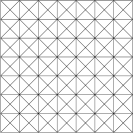
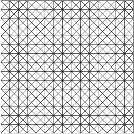
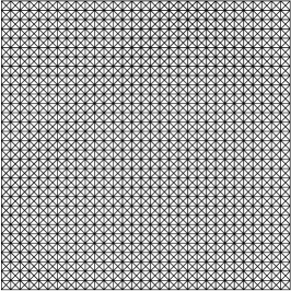
Figure 1: Some meshes from the uniform sequence.

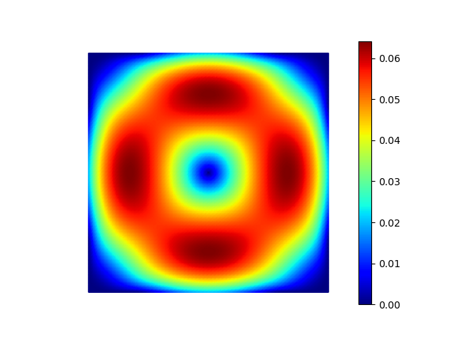
Figure 2: The velocity magnitude (top) and the pressure (bottom) computed using the finest mesh in the uniform sequence.

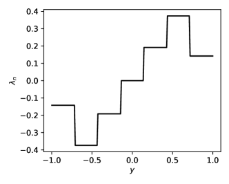
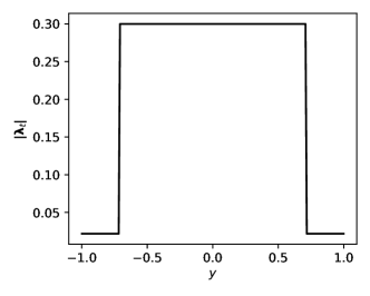
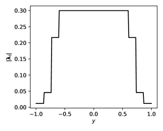
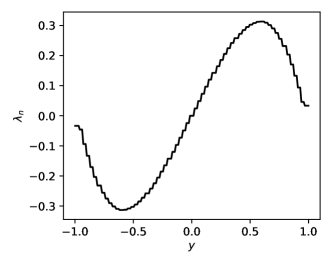
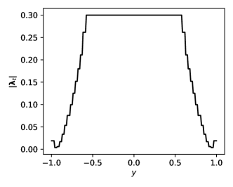
Figure 3: The components of the discrete Lagrange multiplier solution at the boundary $x=1$ plotted for four different meshes from coarsest (top) to finest (bottom).

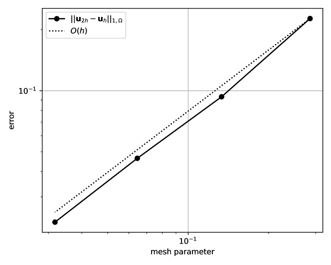
Figure 4: The convergence of the error in the velocity.

Figure 5: The convergence of the error in the pressure.

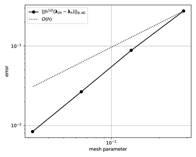
Figure 6: The convergence of the error in the Lagrange multiplier.

References

• [1] M. Ayadi, H. Ayed, L. Baffico, and T. Sassi, Stokes problem with slip boundary conditions of friction type: Error analysis of a four-field mixed variational formulation, Journal of Scientific Computing, 81 (2019), pp. 312–341, https://doi.org/10.1007/s10915-019-01017-x.
• [2] M. Ayadi, L. Baffico, M. K. Gdoura, and T. Sassi, Error estimates for Stokes problem with Tresca friction conditions, ESAIM: M2AN, 48 (2014), pp. 1413–1429, https://doi.org/10.1051/m2an/2014001.
• [3] M. Ayadi, M. K. Gdoura, and T. Sassi, Mixed formulation for Stokes problem with Tresca friction, Comptes Rendus. Mathématique, 348 (2010), pp. 1069–1072.
• [4] H. J. Barbosa and T. J. Hughes, The finite element method with Lagrange multipliers on the boundary: circumventing the Babuška-Brezzi condition, Computer Methods in Applied Mechanics and Engineering, 85 (1991), pp. 109–128.
• [5] J. Djoko and J. Koko, Numerical methods for the Stokes and Navier–Stokes equations driven by threshold slip boundary conditions, Computer Methods in Applied Mechanics and Engineering, 305 (2016), pp. 936–958.
• [6] J. Djoko and J. Koko, GLS methods for Stokes equations under boundary condition of friction type: formulation-analysis-numerical schemes and simulations, SeMA Journal, (2022), pp. 1–29.
• [7] J. Djoko, J. Koko, and S. Konlack, Stokes equations under Tresca friction boundary condition: a truncated approach, Advances in Computational Mathematics, 48 (2022), p. 22, https://doi.org/10.1007/s10444-022-09933-7.
• [8] C. Fang, K. Czuprynski, W. Han, X. Cheng, and X. Dai, Finite element method for a stationary Stokes hemivariational inequality with slip boundary condition, IMA Journal of Numerical Analysis, 40 (2019), pp. 2696–2716, https://doi.org/10.1093/imanum/drz032.
• [9] H. Fujita, A mathematical analysis of motions of viscous incompressible fluid under leak or slip boundary conditions, RIMS Kôkyûroku, 888 (1994), pp. 199–216.
• [10] R. Greve and H. Blatter, Dynamics of ice sheets and glaciers, Springer Science & Business Media, 2009.
• [11] T. Gustafsson, Numerical experiments for ”Stabilised finite element method for Stokes problem with nonlinear slip condition”, Aug. 2023, https://doi.org/10.5281/zenodo.8296578.
• [12] T. Gustafsson and G. D. McBain, scikit-fem: A Python package for finite element assembly, Journal of Open Source Software, 5 (2020), p. 2369, https://doi.org/10.21105/joss.02369.
• [13] T. Gustafsson, P. Råback, and J. Videman, Mortaring for linear elasticity using mixed and stabilized finite elements, Computer Methods in Applied Mechanics and Engineering, 404 (2023), p. 115796.
• [14] T. Gustafsson and J. Videman, Stabilized finite elements for Tresca friction problem, ESAIM: Mathematical Modelling and Numerical Analysis, 56 (2022), pp. 1307–1326.
• [15] J. He and R. Glowinski, Steady Bingham fluid flow in cylindrical pipes: a time dependent approach to the iterative solution, Numerical linear algebra with applications, 7 (2000), pp. 381–428.
• [16] T. Kashiwabara, On a finite element approximation of the Stokes equations under a slip boundary condition of the friction type, Japan Journal of Industrial and Applied Mathematics, 30 (2013), pp. 227–261, https://doi.org/10.1007/s13160-012-0098-5.
• [17] R. Kouhia and R. Stenberg, A linear nonconforming finite element method for nearly incompressible elasticity and Stokes flow, Computer Methods in Applied Mechanics and Engineering, 124 (1995), pp. 195–212.
• [18] C. Le Roux, Steady Stokes flows with threshold slip boundary conditions, Mathematical Models and Methods in Applied Sciences, 15 (2005), pp. 1141–1168, https://doi.org/10.1142/S0218202505000686.
• [19] J. Li, H. Zheng, and Q. Zou, A priori and a posteriori estimates of the stabilized finite element methods for the incompressible flow with slip boundary conditions arising in arteriosclerosis, Advances in Difference Equations, 2019 (2019), p. 374.
• [20] Y. Li and K. Li, Pressure projection stabilized finite element method for Stokes problem with nonlinear slip boundary conditions, Journal of computational and applied mathematics, 235 (2011), pp. 3673–3682.
• [21] F. Pattyn, L. Perichon, A. Aschwanden, B. Breuer, B. De Smedt, O. Gagliardini, G. H. Gudmundsson, R. C. Hindmarsh, A. Hubbard, J. V. Johnson, et al., Benchmark experiments for higher-order and full-Stokes ice sheet models (ISMIP–HOM), The Cryosphere, 2 (2008), pp. 95–108.
• [22] H. Qiu, C. Xue, and L. Xue, Low-order stabilized finite element methods for the unsteady Stokes/Navier-Stokes equations with friction boundary conditions, Mathematical Methods in the Applied Sciences, 41 (2018), pp. 2119–2139.
• [23] N. Saito, On the Stokes equation with the leak and slip boundary conditions of friction type: Regularity of solutions, Publ. Res. Inst. Math. Sci., 40 (2004), pp. 345–383.
• [24] C. Schoof, A variational approach to ice stream flow, Journal of Fluid Mechanics, 556 (2006), pp. 227–251.
• [25] L. Tartar, An introduction to Sobolev spaces and interpolation spaces, vol. 3, Springer Science & Business Media, 2007.
• [26] R. Verfürth, A posteriori error estimators for the Stokes equations, Numerische Mathematik, 55 (1989), pp. 309–325.
• [27] R. Verfürth, A Posteriori Error Estimation Techniques for Finite Element Methods, Oxford University Press, Oxford, 2013, https://doi.org/10.1093/acprof:oso/9780199679423.001.0001.
• [28] B. Wohlmuth, Variationally consistent discretization schemes and numerical algorithms for contact problems, Acta Numerica, 20 (2011), pp. 569–734, https://doi.org/10.1017/S0962492911000079.