Corner Transfer Matrix Approach to the Yang-Lee Singularity in the 2D Ising Model in a magnetic field

Abstract

We study the two-dimensional (2D) Ising model in a complex magnetic field in the vicinity of the Yang-Lee edge singularity. By using Baxter’s variational corner transfer matrix method combined with analytic techniques, we numerically calculate the scaling function and obtain an accurate estimate of the location of the Yang-Lee singularity. The existing series expansions for susceptibility of the 2D Ising model on a triangular lattice by Chan, Guttmann, Nickel, and Perk allowed us to substantially enhance the accuracy of our calculations. Our results are in excellent agreement with the Ising field theory calculations by Fonseca, Zamolodchikov and the recent work by Xu and Zamolodchikov. In particular, we numerically confirm an agreement between the leading singular behavior of the scaling function and the predictions of the ${\mathcal{M}}_{2/5}$ conformal field theory.

DOI:10.1103/PhysRevE.108.064136

I Introduction

The two-dimensional (2D) Ising model plays a prominent role in the development of the theory of phase transition and critical phenomena [1, 2, 3, 4, 5, 6, 7, 8, 9, 10]. In Refs. [11, 12] the scaling and universality of the 2D Ising model in a magnetic field were studied by Baxter’s corner transfer matrix approach [4]. Here we further continue this study. We consider the planar nearest-neighbour Ising model on regular square and triangular lattices. Its partition function reads

$${Z}=\sum_{\sigma}\exp\{\,\beta\sum_{\langle ij\rangle}\sigma_{i}\sigma_{j}+{H}\sum_{i}\sigma_{i}\,\Big{\}}\ ,\quad\sigma_{i}=\pm 1,$$ (1)

where the first sum in the exponent is taken over all edges, the second sum — over all sites and the outer sum — over all spin configurations $\{\sigma\}$ of the lattice. The constants $H$ and $\beta=J/k_{B}T$ denote the (suitably normalized) magnetic field and inverse temperature. The free energy, magnetization and magnetic susceptibility are defined as

$$f=-\lim_{N\to\infty}\frac{1}{N}\log Z,\quad M=-\frac{\partial f}{\partial H},\quad\chi=-\frac{\partial^{2}f}{\partial H^{2}}\ ,$$ (2)

where $N$ is the number of lattice sites and derivatives are taken at zero field $H=0$. The model exhibits a second order phase transition at $\beta=\beta_{c}$ and $H=0$, where

$$\beta_{c}^{(s)}={\textstyle{\frac{1}{2}}}\log(1+\sqrt{2}),\qquad\beta_{c}^{(t)}={\textstyle{\frac{1}{4}}}\log 3,$$ (3)

for the square [1] and triangular [13] lattices, respectively. Since we investigate the large lattice limit, boundary conditions become irrelevant in the off-critical regime. We shall be using the fixed boundary conditions, which are naturally arising in the corner transfer matrix method.

It is convenient to introduce a new temperature-like variable $\tau$

$${\tau=\frac{1}{2}\left(\sqrt{k}-\frac{1}{\sqrt{k}}\right)},\quad k=(\tau+\sqrt{1+\tau^{2}})^{2}$$ (4)

defined via the “elliptic modulus” parameter $k$. The latter is connected to the inverse temperature $\beta$ through the following lattice-dependent formulas [8]

$$k^{(s)} =\frac{1}{s^{2}},\quad s=\sinh 2\beta^{(s)},$$ (5)

$$k^{(t)} =\frac{4t^{3/2}}{(1-t)^{3/2}(1+3t)^{1/2}},\quad t=e^{-4\beta^{(t)}},$$ (6)

where the superscripts $(s)$ and $(t)$ stand for the square and triangular lattices, respectively.

The temperature variable $\tau$ is inspired by the Kramers-Wannier duality transformation $\tau\to-\tau$ and $k\to 1/k$ around the critical point $\tau=0$. The high temperature regime corresponds to $\tau>0$ and $k>1$.

Close to the critical point $\tau,H\to 0$, the singular part of the lattice free energy, $f_{\textrm{sing}}$, dominates the free energy $f$ due to a logarithmic singularity. It has the form

$$f_{\textrm{sing}}(\tau,H) =\frac{m^{2}}{8\pi}\log[m^{2}]+m^{2}G(\xi),\>\>\xi=\frac{h}{|m|^{15/8}},$$ (7)

where $m$ and $h$ are specially constructed nonlinear scaling variables [14] whose leading terms for small $\tau,H\to 0$ are proportional to $\tau$ and $H$, respectively, see Eq. (10) below. The universality implies that the scaling function $G$ depends on $h$ and $m$ only via the ratio $\xi$ defined in Eq. (7). Analytic properties of the scaling function $G(\xi)$ in the complex plane $\xi$ have been thoroughly analized in Ref. [9].

In this paper, we investigate a detailed structure of $G(\xi)$ in the neighborhood of the so-called Yang-Lee edge singularity [15, 16]. In particular, we give a very accurate estimate for the location of this singularity, extending the recent results of Ref. [10].

The paper is organised as follows. In Sec. II we give a brief exposure of the Ising scaling theory, discuss different critical regimes and describe our approach. We also explain the benefits of working with a triangular lattice instead of the square one. In Sec. III we review known analytic results for the Ising model at zero magnetic field on a triangular lattice. We use them to determine certain parts of the free energy in the thermodynamic limit. The calculations of the magnetic susceptibility are reviewed in Sec. IV. In Sec. V we explain the corner transfer matrix method and its modification for the triangular lattice. In Sec. VII we present all numerical results which we used to determine the expansion of the scaling function near the Yang-Lee singularity. Finally, in Conclusion we discuss the results and make some comments on unsolved problems.

II Scaling theory

According to the scaling theory, the lattice free energy (2) in the vicinity of the critical point $\tau,H\to 0$ can be written as

$$f(\tau,H) =f_{\textrm{sing}}(\tau,H)+f_{\textrm{reg}}(\tau,H)+f_{\textrm{sub}}(\tau,H),$$ (8)

where the leading singular part

$$f_{\textrm{sing}}(\tau,H)=\mathcal{F}(m(\tau,H),h(\tau,H)),$$ (9)

can be expressed through a universal scaling function $\mathcal{F}(m,h)$, with the parameters $\tau$ and $H$ entering the right-hand side (RHS) of Eq. (9) only through nonlinear scaling variables [14]

$$m(\tau,H) =-C_{\tau}\,a(\tau)\,\tau+\mu_{h}\,H^{2}b(\tau)+\mathcal{O}(H^{4}),$$

$$h(\tau,H) =C_{H}\,c(\tau)\,H+e_{h}\,d(\tau)\,H^{3}+\mathcal{O}(H^{5}).$$ (10)

Note, that all the constants and coefficient functions in the above formulas are lattice dependent. Here we assume the following normalization

$$a(\tau)=1+O(\tau),\quad b(\tau)=1+O(\tau),$$

$$c(\tau)=1+O(\tau),\quad d(\tau)=1+O(\tau).$$ (11)

with $C_{\tau}>0,\,C_{H}>0$. The leading singular part (9) has the form

$$\mathcal{F}(m,h) =\frac{m^{2}}{8\pi}\log[m^{2}]+m^{2}G(\xi),\>\>\xi=\frac{h}{|m|^{15/8}}.$$ (12)

which was already quoted in Eq. (7). Next, the regular part $f_{\textrm{reg}}(\tau,H)$ in Eq. (8) contains no singularities at $\tau,H\to 0$ and have the following Taylor expansion

$$f_{\textrm{reg}}(\tau,H) =A(\tau)+H^{2}B(\tau)+\mathcal{O}(H^{4}).$$ (13)

The last term $f_{\textrm{sub}}(\tau,H)$ in Eq. (8) denotes the less singular than $f_{\textrm{sing}}(\tau,H)$ part. It can be written as

$$f_{\textrm{sub}}(\tau,H)=H^{2}f_{\textrm{sub}}(\tau)+O(H^{4}).$$ (14)

The first nontrivial contribution to $f_{\textrm{sub}}(\tau)$, associated with irrelevant operators in the Ising CFT [17], will be determined from the susceptibility calculations of ref. [8].

Analytic properties of the scaling function $G(\xi)$ for complex $\xi$ have been discussed in details in Refs. [9, 10]. In fact, to describe $\mathcal{F}(m,h)$ for both positive and negative $m$ it is convenient to use two different (but, of course, related) scaling functions in Eq. (12). In the high-temperature regime $m<0$ the scaling function $G(\xi)$ admits a series expansion

$$G_{\textrm{high}}(\xi)=G_{2}\xi^{2}+G_{4}\xi^{4}+G_{6}\xi^{6}+G_{8}\xi^{8}+\ldots.$$ (15)

convergent in some domain around the origin $\xi=0$. Note, that this expansion contains only even powers of $\xi$, since for $m<0$ there is a symmetry $H\to-H$.

In the low-temperature regime $m>0$, the scaling function admits an asymptotic expansion for small $\xi$

$$G_{\textrm{low}}(\xi)=\tilde{G}_{1}\xi+\tilde{G}_{2}\xi^{2}+\tilde{G}_{3}\xi^{3}+\tilde{G}_{4}\xi^{4}+\ldots.$$ (16)

containing all powers of $\xi$. Coefficients $G_{i}$ and $\tilde{G}_{i}$ are universal for all lattices [12]. The first few of these coefficients are known with a very high accuracy [11]. For later use, in Table 1 we quote the coefficients $G_{n}$ with $n\leq 10$.

Table 1: Values of coefficients $G_{n}$

$G_{2}$ aa	$-1.84522807823(1)$
$G_{4}$	$\phantom{+}8.3337117508(1)$
$G_{6}$	$-95.16897(3)$
$G_{8}$	$\phantom{+}1457.62(3)$
$G_{10}$—	$-25891(2)$

Next, it is convenient to introduce another scaling variable

$$\eta=\frac{m}{h^{8/15}}$$ (17)

and rewrite Eq. (12) as

$$\mathcal{F}(m,h)=\frac{m^{2}}{8\pi}\log[m^{2}]+h^{16/15}\Phi(\eta).$$ (18)

Then for the high-temperature regime one obtains

$$\Phi(\eta)=\eta^{2}G_{\textrm{high}}((-\eta)^{-15/8})\quad\mbox{for real}\quad\eta<0.$$ (19)

The function $\Phi(\eta)$ admits the expansion for small $\eta$ [9]

$$\Phi(\eta)=-\frac{\eta^{2}}{8\pi}\log\eta^{2}+\sum_{k=0}^{\infty}\Phi_{k}\eta^{k},$$ (20)

where the series converges in a finite domain around the origin of the complex $\eta$-plane. The first two coefficients $\Phi_{0}$ and $\Phi_{1}$ are known exactly, thanks to the integrability of the critical Ising field theory in a magnetic field [7]. The higher coefficients $\Phi_{k}$, with $k\leq 8$ are known numerically, see Refs. [9, 11].

From the high-temperature regime the function $G_{\textrm{high}}(\xi)$ can be analytically continued to complex values of $\xi$. The Yang-Lee theory [15, 16] guarantees analyticity of $G_{\textrm{high}}(\xi)$ in the complex $\xi$-plane with two branch cuts $(-i\infty,-i\xi_{0})$ and $(i\xi_{0},+i\infty)$ on the imaginary axis. These cuts arise from a condensation of the Yang-Lee zeros of the partition function in the thermodynamic limit [18]. In this paper, we study the neighborhood of the Yang-Lee edge singularity at $\xi=\pm i\xi_{0}$, which is another critical point of the Ising model (1) associated with the nonunitary minimal CFT model ${\cal M}_{2/5}$ with the central charge $c=-22/5$ [19, 20], often named as “Yang-Lee” CFT (YLCFT). It has only one primary field $\phi$ with the scaling dimension $2\Delta=-2/5$. To analyse this critical point, one needs to consider the ${\cal M}_{2/5}$ CFT perturbed by the relevant operator $\phi$ together with an infinite number of irrelevant operators. Further details are given in Sec. VII.

The suggested numerical value of $\xi_{0}$ in Ref. [9] is

$$\xi_{0}=0.18930(5).$$ (21)

In this paper, we numerically calculate the scaling function to study its expansion near the singularity and, in particular, significantly improve the above estimate for $\xi_{0}$, see Eq. (101) below.

Our strategy is as follows. We consider the lattice Ising model in the high-temperature regime with a complex magnetic field $H$ in the neighborhood of the Yang-Lee edge singularity, $\xi=\pm i\xi_{0}$, with $\xi_{0}$ given by Eq. (21). Using the numerical corner transfer matrix algorithm, we calculate the lattice free energy $f_{\textrm{ctm}}(\tau,H)$ with relatively high accuracy (at least 15 decimal places) for a large set of numerical values of the temperature and magnetic field.

Using Eqs. (8) and (12), one can express the scaling function as

$$G(\xi)=\frac{1}{m^{2}}\big{(}f_{\textrm{ctm}}(\tau,H)-\frac{m^{2}}{8\pi}\log[m^{2}]$$

$$-f_{\textrm{reg}}(\tau,H)-f_{\textrm{sub}}(\tau,H)\big{)},$$ (22)

where all functions in the RHS are given by series in $\tau$ and $H$ and can be determined from analytic results and numerical calculations in the high/low-temperature regimes.

Consider the high-temperature regime $m<0$ and fix the variable $\xi$. Then using Eq. (7) the scaling variable $h$ can be written as

$$h(\tau,H)=\big{(}-m(\tau,H)\big{)}^{15/8}\,\xi.$$ (23)

Combining this with Eq. (10) one can invert the series in $H$ and obtain the following expansion

$$H(\tau)=\xi\,\tau^{15/8}\,\sum_{k=0}^{\infty}\xi^{2k}\,\tau^{11k/4}\,p_{k}(\tau),$$ (24)

where $p_{k}(\tau)$ are regular in $\tau$. Then it is easy to see that the coefficients of a series expansion of $H(\tau)$ in powers of $\tau$ are finite polynomials in $\xi$. Thus, the variable $\xi$ can be assigned to any fixed value — not necessarily small.

Substituting Eq. (24) into the RHS of Eq. (22) one obtains a function of two variables $\xi$ and $\tau$, which should not depend on $\tau$. This is a highly nontrivial self-consistency test that determines the accuracy of the calculation of $G(\xi)$. Indeed, taking two different values of $\tau$ with a fixed $\xi$, one should get the same value of $G(\xi)$.

The CTM method can be applied to regular square, triangular, or honeycomb lattices. As was shown in Refs. [17, 8], for the Ising model the CTF irrelevant operators contribute in the order $\tau^{4}$ for the square lattice and in the order $\tau^{6}$ for the triangular/honeycomb lattices. This implies that one can achieve much better accuracy for the triangular lattice [12]. For this reason, we restrict all further analysis to this case.

The precision of CTM calculations is limited by the machine accuracy, which in our case is $10^{-16}$. As we shall see below, for the triangular lattice one can reliably control the series expansion coefficients in the RHS of Eq. (22) up to the order of $\tau^{8}$. Therefore, there is an upper limit on the value of $\tau$ for which the unknown higher terms in Eq. (22) do not affect the precision of calculations. Having this in mind, one needs, nonetheless, to choose $\tau$ as large as possible to speed up the convergence of the CTM algorithm. The latter is mainly determined by the variable

$$\Delta\beta=\beta_{c}^{(t)}-\beta=\textstyle\frac{1}{4}\tau+O(\tau^{2}).$$ (25)

Numerical experiments suggest that the optimal value of $\Delta\beta$ for the maximum precision calculations should be in the range

$$0.006\leq\Delta\beta\leq 0.012\,,$$ (26)

where the lower bound is near the boundary of convergence of the CTM algorithm. To reach the numerical accuracy of $10^{-15}$ the calculations were performed with corner transfer matrices of the size $N=170$.

Since the RHS of Eq. (22) contains an extra factor $1/m^{2}$, the accuracy of calculations of $G(\xi)$ is reduced by four or five decimal places. Therefore, one can expect the accuracy of the scaling function to be around $10^{-10}$. Indeed, we calculated $G(\xi)$ for a large set of points $\xi_{i}$ in the complex plane with three values of $\Delta\beta$,

$$\Delta\beta=0.006,\ 0.007,\ 0.012\,,$$ (27)

corresponding to

$$\tau\simeq 0.024,\ 0.028,\ 0.048\,.$$ (28)

A difference between the values of $G(\xi)$ for these values of $\tau$ never exceeded $2.\times 10^{-10}$. Therefore, it suggests that this is the accuracy of our calculations of the scaling function $G(\xi)$.

III Ising model with $H=0$ on a triangular lattice

In this and the next sections we will use all available exact and perturbation theory results for the 2D lattice Ising model to determine the lattice-dependent regular (13) and subleading (14) contributions to the free energy, as well as to find coefficients entering the nonlinear scaling variables (10) to highest possible orders in the variables $\tau$ and $H$.

The free energy of the Ising model on the triangular lattice can be written in the form of the following integral [13]

$$f^{(t)}(\tau,0)=-\frac{1}{2}\log(4\sinh 2\beta)-\frac{1}{8\pi^{2}}\iintop\ilimits@\limits_{0}^{2\pi}d\phi_{1}d\phi_{2}$$

$$\times\log[r(\beta)-\cos\phi_{1}-\cos\phi_{2}+\cos(\phi_{1}+\phi_{2})],$$ (29)

where

$$r(\beta)=\frac{3+e^{8\beta}}{2(e^{4\beta}-1)}$$ (30)

and $\beta$ and $\tau$ are related through Eqs. (4) and (6).

At $\tau=0$ the integral in Eq. (29) can be evaluated explicitly

$$f^{(t)}(0,0)=-\frac{5}{2\pi}\mbox{Cl}_{2}\left(\frac{\pi}{3}\right)-\frac{1}{4}\log\frac{4}{3},$$ (31)

where $\mbox{Cl}_{2}(x)$ is the Clausen function,

$$\mbox{Cl}_{2}\left(\frac{\pi}{3}\right)\approx 1.0149416064096536.$$ (32)

To calculate the expansion of $f^{(t)}(\tau,0)$ for small $\tau>0$ we first calculate the derivative of Eq. (29) with respect to $\beta$. It can be expressed in terms of the complete elliptic integral of the first kind

$$\frac{df^{(t)}(\tau,0)}{d\beta}=\frac{e^{2\beta}(e^{4\beta}-3)}{\pi\tanh 2\beta}K(1/k)$$ (33)

and $k$ is given by Eq. (6).

From Eqs. (4) and (6) we can express $\Delta\beta$ in Eq. (25) as series in $\tau$

$$\Delta\beta= \frac{\tau}{4}-\frac{\tau^{2}}{16}-\frac{11\tau^{3}}{192}+\frac{7\tau^{4}}{256}+\frac{39\tau^{5}}{1280}-\frac{205\tau^{6}}{12288}$$

$$- \frac{1165\tau^{7}}{57344}+\frac{767\tau^{8}}{65536}+\frac{8887\tau^{9}}{589824}+O(\tau^{10}).$$ (34)

Expanding Eq. (33) for small $\tau>0$ and integrating, we arrive at the high-temperature expansion of the free energy (29) at $H=0$

$$f^{(t)}(\tau,0)=\frac{m^{2}(\tau,0)}{8\pi}\log m^{2}(\tau,0)+A(\tau),$$ (35)

$$m(\tau,0)=-C_{\tau}\tau a(\tau),\quad C_{\tau}=\frac{3^{3/4}}{\sqrt{2}},$$ (36)

Comparing this with Eq. (10), we obtain series expansions for the functions $a(\tau)$ and $A(\tau)$

$$a(\tau)= 1-\frac{3\tau^{2}}{16}+\frac{23\tau^{4}}{256}-\frac{229\tau^{6}}{4096}$$

$$+\frac{25819\tau^{8}}{655360}+\mathcal{O}(\tau^{10}),$$ (37)

$$A(\tau)=-\frac{5}{2\pi}\mbox{Cl}_{2}\left(\frac{\pi}{3}\right)-\frac{1}{4}\log\frac{4}{3}+\frac{\tau}{2}-\frac{\tau^{3}}{12}+\frac{3\tau^{5}}{80}$$

$$-\frac{5\tau^{7}}{224}+\frac{35\tau^{9}}{2304}+\frac{\tau^{2}}{32}\left[2-\frac{3\sqrt{3}(2+3\log 12)}{\pi}\right]$$

$$+\frac{\tau^{4}}{256}\left[-7+\frac{3\sqrt{3}(5+9\log 12)}{\pi}\right]+$$

$$+\frac{\tau^{6}}{8192}\left[\frac{410}{3}-\frac{9\sqrt{3}(28+55\log 12)}{\pi}\right]+$$

$$+\frac{\tau^{8}}{65536}\left[-767+\frac{\sqrt{3}(1291+2682\log 12)}{\pi}\right]+\ldots$$ (38)

Using the exact expression for a zero-field magnetization for $\tau<0$

$$M=(1-k^{2})^{1/8},$$ (39)

we find the expression for the function $c(\tau)$ in Eq. (10)

$$c(\tau)=-\frac{M(\tau)}{C_{H}\tilde{G}_{1}(-C_{\tau}\tau a(\tau))^{1/8}},$$ (40)

where the coefficient $\tilde{G}_{1}$ from Eq. (16) is known [3]

$$\tilde{G}_{1}=-2^{1/12}\,e^{-1/8}\,{\mathcal{A}}^{3/2}=-1.357838341706595\ldots\ ,$$ (41)

and ${\mathcal{A}}=1.282427\ldots$ is the Glaisher constant.

Using Eqs. (4) and (6), we can also expand $k(\tau)$ in $\tau$

$$k(\tau)=1+2\tau+2\tau^{2}+\tau^{3}-\frac{\tau^{5}}{4}+\frac{\tau^{7}}{8}-\frac{5\tau^{9}}{64}+O(\tau^{11}).$$ (42)

Combining Eqs. (39–42), we finally obtain

$$C_{H}=\frac{2^{11/48}e^{1/8}}{3^{3/32}{\mathcal{A}}^{3/2}}=0.825075494181738\ldots,$$ (43)

$$c(\tau)=1+\frac{\tau}{4}+\frac{15\tau^{2}}{128}-\frac{9\tau^{3}}{512}-\frac{1447\tau^{4}}{32768}+\frac{649\tau^{5}}{131072}$$

$$+\frac{109293\tau^{6}}{4194304}-\frac{29803\tau^{7}}{16777216}-\frac{194751097\tau^{8}}{10737418240}+O(\tau^{9}).$$ (44)

IV Susceptiblity

Our analysis greatly relies on the availability of the high order perturbation theory calculations of the magnetic susceptibility in the Ising model on the triangular lattice [8]. As mentioned before, the first nontrivial contribution from the CFT irrelevant operators in this case comes only at the order $\tau^{6}$ and this helps to obtain very accurate results for the scaling function. First, we start with our definition of susceptibility $\eqref{F-def}$ with the free energy given by $\eqref{lab2}$. For simplicity, we consider the high-temperature regime $\tau>0$. Substituting Eqs. (10), (12), (13), and (14) into Eq. (8) and differentiating over $H$ twice one obtains,

$$\chi(\tau)= -\frac{2C_{H}^{2}G_{2}}{C_{\tau}^{7/4}\tau^{7/4}}\frac{c(\tau)^{2}}{a(\tau)^{7/4}}-2(B(\tau)+f_{\textrm{sub}}(\tau))$$

$$+\frac{C_{\tau}\mu_{h}\tau a(\tau)b(\tau)}{2\pi}(1+2\log(c_{\tau}\tau a(\tau))),$$ (45)

where $G_{2}$ is the first expansion coefficient in the scaling function $G_{\textrm{high}}(\xi)$ and given in Table 1. It was evaluated with a very high accuracy in Ref. [21].

The first term in Eq. (45) describes the contribution of the Aharony and Fisher scaling function [14] on a triangular lattice

$$F_{AF}(\tau)=\frac{c(\tau)^{2}}{a(\tau)^{7/4}}=k^{1/4}\biggl{[}1+\frac{\tau^{2}}{2}-\frac{21\tau^{4}}{256}$$

$$+\frac{85\tau^{6}}{2048}-\frac{8669\tau^{8}}{327680}+\frac{49507\tau^{10}}{2621440}+O(\tau^{12})\biggr{]}$$ (46)

and the coefficient $C_{0}$

$$C_{0}=-\frac{2C_{H}^{2}G_{2}}{C_{\tau}^{7/4}}=1.089549651052967\ldots$$ (47)

coincides with $C_{0\pm}^{\mbox{\scriptsize tr}}$ from Ref. [8].

Now let us give the expression for the Ising susceptibility on a triangular lattice [8]. It can be written in the form

$$\chi_{\mbox{\scriptsize CGNP}}(\tau)=C_{0}\tau^{-7/4}F_{lat}(\tau)+B_{lat}(\tau),$$ (48)

$$B_{lat}(\tau)=\sum_{p=0}^{\infty}b_{p,q}(\log\tau)^{p}\tau^{p^{2}}B_{p}(\tau),$$ (49)

where $B_{p}(\tau)$ are regular in $\tau$. Let us note that the term with $p=3$ starts with the lowest power $\tau^{9}$ and its contribution to the scaling function is of the order $H^{2}\tau^{9}\sim\xi^{2}\tau^{11+3/4}$. Functions $B_{p}(\tau)$, $p=0,1,2$ are given in Appendix C.3 of Ref. [8] and we will not list them here.

We have

$$F_{lat}(\tau)=F_{AF}(\tau)+\Delta F,$$ (50)

$$\Delta F=k^{1/4}[c_{6}\tau^{6}+c_{8}\tau^{8}+c_{10}\tau^{10}+O(\tau^{12})],$$ (51)

$$c_{6}=- 0.1774838832948664\ldots,$$

$$c_{8}=- \frac{1}{102400}-\frac{403}{400}c_{6}$$

$$= 0.1788052467945779\ldots,$$

$$c_{10}=- 0.1488704025260859\ldots$$ (52)

The term $\Delta F$ comes from CFT irrelevant operators and contributes to the subleading part $f_{\textrm{sub}}(\tau)$.

Finally, comparing Eqs. (45) and (48) we can determine $\mu_{h}$, $b(\tau)$, $B(\tau)$ and $f_{\textrm{sub}}(\tau)$. We give them up to the order $\tau^{5}$, further terms’ contributions to the free energy are less than $10^{-15}$. We also restrict accuracy of the coefficients to $10^{-10}$ because all these functions are multiplied by $H^{2}\sim\tau^{15/4}\approx 10^{-6}$ for values of $\tau\approx 0.025$.

$$\mu_{h}=-0.01047478006\ldots,$$ (53)

$$b(\tau)= 1+\frac{\tau}{2}+0.122460779\,\tau^{2}+9.228424771\,\tau^{3}$$

$$-4.710909908\,\tau^{4}+6.54812548\,\tau^{5}+\ldots,$$ (54)

$$B(\tau)= 0.02478055826+0.02444328450\tau$$

$$+ 0.01102511536\tau^{2}-0.001283871801\tau^{3}$$

$$- 0.07567570347\tau^{4}-0.03469707085\tau^{5}+\ldots.$$ (55)

Contributions to $f_{\textrm{sub}}(\tau)$ come from $\Delta F$ in (51) and terms proportional to $(\log\tau)^{2}$ in Eq. (49). We have

$$f_{\textrm{sub}}(\tau)=1.089549651\,\tau^{\frac{17}{4}}(1+\frac{\tau}{2}+0.8824449774\tau^{2})$$

$$-0.0041507859(\log\tau)^{2}\tau^{4}(1+\frac{\tau}{2}-0.8222691101\tau^{2}).$$ (56)

Let us also notice that for $\tau\approx 0.025$ a contribution from the sub-leading term (56) to the scaling function $G(\xi)$ is of the order $10^{-8}$.

Finally, we need to determine $e_{h}$ and $d(\tau)$ in Eq. (10). The value of the constant $e_{h}$ was accurately estimated in Ref. [12]

$$e_{h}=0.00129(1).$$ (57)

Since $e_{h}H^{3}=e_{h}\xi^{3}\tau^{45/8}\approx 10^{-14}$ for $\tau=0.025$ and $\xi=0.2$, we can expect that the linear term in $d(\tau)$ will give a contribution $\sim 10^{-16}$ to the free energy. We will neglect it and simply choose

$$d(\tau)=1.$$ (58)

It should not affect the accuracy of the scaling function $G(\xi)$.

V CTMRG

Corner transfer matrices (CTM) have proven to be an effective tool for numerical study of lattice systems in 2D [22, 23, 24]. Nishino et al. [25] introduced an improved iteration scheme for the original Baxter approach, now known as the corner transfer matrix renormalization group (CTMRG). In this section we shall give a brief introduction to this method.

We first formulate the algorithm for a square lattice in the Interaction-Round-Face (IRF) formulation. Although this is not essential for the algorithm, we assume that all spins take two values, $+1$ and $-1$.

First, we introduce the four-spin Boltzmann weight $w(a,b,c,d)$ as in Fig. 1.

Figure 1: The four-spin weight $w(a,b,c,d)$.

For a symmetric square lattice Ising model we have

$$w(a,b,c,d)=e^{\frac{\beta}{2}(ab+ac+bd+cd)+\frac{H}{4}(a+b+c+d)}.$$ (59)

The factors $1/2$ and $1/4$ enter Eq. (59) because each edge is shared by two plaquettes and each vertex is shared by four plaquettes of the square lattice.

Now we define a half-row transfer matrix (HRTM) $F(a,b)_{i,j}$. For the transfer matrix of the length $N+2$ we fix the leftmost spins as $(a,b)$, the rightmost spins as $(+1,+1)$ and combine the remaining spins into multi-indices $i$ and $j$

$$i=\{i_{1},\ldots,i_{N}\},\quad j=\{j_{1},\ldots,j_{N}\}$$ (60)

as shown in Fig. 2.

Figure 2: The half-row transfer matrix $F(a,b)_{i,j}$

The rightmost spins $(+1,+1)$ play the role of boundary conditions and we will always fix boundary spins to $+1$ values. For 2D models out of criticality, the choice of boundary spins should become irrelevant in the thermodynamic limit. In general, we also need a half-column transfer matrix $G(a,b)$. However, in the symmetric case $F(a,b)$ and $G(b,a)$ are related by the matrix transposition, see (63).

Now we define the corner transfer matrix (CTM) $A(a)_{i,j}$, see Fig. 3. Its rightmost and topmost indices are fixed to $+1$, the bottom and left spins are combined into matrix indices $i$ and $j$ except the corner spin $a$.

Figure 3: The corner transfer matrix $A(a)_{i,j}$

We also sum over all internal spins shown by black circles. Here and below we follow the notation, that the spins denoted by white circles (or rectangles for multi-indices) are fixed, while the spins denoted by black circles/rectangles are summed over.

Notice that the $2^{N}\times 2^{N}$ corner transfer matrix $A(a)$ is nothing but the partition function of the model on the $(N+2)\times(N+2)$ square lattice with fixed boundary conditions.

The main idea of the CTMRG method is to calculate $A(a)$ recursively and truncate it at each step to physically relevant degrees of freedom.The core of the algorithm relies on the insight that the eigenvalues of the transfer matrix decay exponentially fast in the off-critical regime, so the vast majority of the information about the CTMs is contained in a finite set of dominant eigenvalues. At each step, the iteration algorithm doubles the size of $A$ and $F$, but since the majority of information is contained in the largest eigenvalues, the smaller half of eigenvalues can be discarded with minimal information loss while reducing the size of the matrix to its original size.

We can summarize the algorithm by the following steps.

1. We start the algorithm with the initialization of matrices $A$ and $F$. It is easy to calculate them for small-size lattices. We could even initialize them as random matrices with positive entries, this does not much affect the convergence of the algorithm.

2. We update the CTM $A(a)_{i,j}$ to the expanded CTM $A^{\prime}(a)_{I,L}$ of a double size as shown in Fig. 4.

Figure 4: The updated matrix $A^{\prime}(a)_{I,L}$

This can be written as

$$A^{\prime}(a)_{I,L}=\sum_{d,j,k}w(b,d,a,c)F(c,d)_{ij}A(d)_{j,k}G(d,b)_{k,l}$$ (61)

with $I=\{c,i\}$, $L=\{b,l\}$.

If the weights $w(a,b,c,d)$ satisfy the symmetry

$$w(a,b,c,d)=w(d,b,c,a),$$ (62)

then the CTM $A(a)$ will be a symmetric matrix and the half-column matrix transfer matrix $G(a,b)$ is a transposition of $F(b,a)$

$$G(a,b)_{i,j}=F(b,a)_{j,i}.$$ (63)

We update the HRTM $F(a,b)$ by simply adding another weight $w$ on the left. After several iterations we arrive at matrices of reasonable sizes the computer can still handle reasonably well, say $64\times 64$.

3. Now we diagonalize $A^{\prime}(a)$ for $a=\pm 1$

$$A^{\prime}(a)=U(a)A^{\prime}_{d}(a)U^{-1}(a).$$ (64)

For a real magnetic field, the matrix $A^{\prime}(a)$ is a real symmetric matrix. Therefore, the matrix $U(a)$ can be chosen orthogonal. The columns of $U(a)$ are the eigenvectors of $A^{\prime}(a)$.

In this paper we investigate the Ising model in a complex magnetic field $H$. The CTM in this case will be a complex symmetric matrix. Its eigenvalues $A^{\prime}_{d}(a)$ in Eq. (64) will, in general, be complex. We will order them by their absolute value. The numerical calculations clearly show that all these eigenvalues are non-degenerate (as it would reasonably be expected). Note also, that the matrix $U(a)$ in Eq. (64) in this case will no longer be orthogonal or unitary.

As explained in Sec. II, for a fixed value of the temperature-like parameter $\tau$ the free energy of the model is an analytic function of the magnetic field $H$ in the cut plane with the branch cuts associated with Yang-Lee edge singularity. We have carefully investigated a stability of our calculations with respect to small imaginary variations of the magnetic field. The results were always consistent and independent of the path chosen to approach complex values of $H$ starting from the purely real ones, as long as the path does not cross the Yang-Lee branch cuts.

4. If the dimension of the original CTM $A(a)$ is $N$, then the dimension of the updated matrix $A^{\prime}(a)$ will be $2N$. We now select first $N$ eigenvalues of $A^{\prime}_{d}(a)$ and form $2N\times N$ matrix from the eigenvectors

$$V(a)_{I,j}=U(a)_{I,j},\quad I=1,\ldots,2N,\quad j=1,\ldots N.$$ (65)

We notice that the first index of $V(a)$ still has the tensor structure $I=\{c,i\}$ inherited from Eq. (61).

Now we form new $N\times N$ CTM $A_{n}(a)$ and HRTM $F_{n}(a,b)$

$$A_{n}(a)_{i,j}=\delta_{ij}A^{\prime}_{d}(a)_{i,i},\quad i,j=1,\ldots,N$$ (66)

$$F_{n}(a,b)_{k,l}=\sum_{c,d,i,j}w(b,d,a,c)$$

$$\times V^{T}(a)_{k,\{c,i\}}F(c,d)_{i,j}V(b)_{\{d,j\},l}$$ (67)

as shown in Fig. 5.

Figure 5: The updated matrix $F_{n}(a,b)$

5. Then we go back to step 2 and repeat iterations until the process converges. We may also increase the size $N$ of the transfer matrices to get a better convergence. We used Intel Fortran with the maximum value $N=170$ to achieve the error comparable with the machine accuracy $10^{-16}$ for a range of temperatures and magnetic fields near the Yang-Lee singularity.

It is possible to achieve a much higher accuracy with larger values of $N$ performing calculations with quad precision. For example, in the high-temperature regime, our numerical free energy matched the Onsager’s result with $10^{-25}$ accuracy. However, this will not improve the accuracy of the scaling function because we need to know series in $\tau$ to higher orders which are determined by irrelevant operators and very hard to control.

VI Partition function per site

Once we calculated the CTM $A$ and the HRTM $F$, we can calculate the partition function per cite following Baxter’s variational arguments [22, 23]. We shall refer the interested reader to the original Baxter’s papers and first give the result for a square lattice. The partition function per site $\kappa$ is given by

$$\kappa=\frac{r_{1}r_{4}}{r_{2}r_{3}}$$ (68)

with each term on the right given explicitly by

$$r_{1}=\sum_{a} \Tr[A(a)^{4}]$$

$$r_{2}=\sum_{a,b} \Tr[A(a)^{2}F(a,b)A(b)^{2}F(b,a)]$$

$$r_{3}=\sum_{a,b} \Tr[A(a)^{2}F(b,a)^{T}A(b)^{2}F(a,b)^{T}]$$

$$r_{4}=\sum_{a,b,c,d} w(a,b,c,d)\Tr\left[A(a)F(a,c)A(c)F(d,c)^{T}\right.$$

$$\left.A(d)F(d,b)A(b)F(a,b)^{T}\right].$$ (69)

For the symmetric Ising model, $A(a)$ is symmetric and

$$F(a,b)=F(b,a)^{T}.$$ (70)

Now let us discuss the case of the symmetric Ising model on a triangular lattice. We can reduce the CTMRG algorithm to the square lattice one by choosing the weight in the form

$$w(a,b,c,d)=e^{\frac{\beta}{2}(ab+ac+bd+cd+2ad)+\frac{H}{6}(2a+b+c+2d)},$$ (71)

see Fig. 6.

Figure 6: The four-spin weight $w(a,b,c,d)$ for a triangular lattice.

The square lattice CTMRG algorithm will still work since the weight (71) satisfies the property (62) and the matrix $A(a)$ is symmetric. However, the matrix $F(a,b)$ no longer satisfies the property (70) and we need to use $F^{T}$. We also need to modify a calculation of the partition function per site.

First, we draw a triangular lattice in the form of four parts separated by bold lines where each dashed rectangle is identified with the weight (71). We can identify this with a square lattice with two transfer matrices $A(a)$ and $B(a)$ assigned to different quadrants, see Fig. 7.

Figure 7: CTMs for a triangular lattice.

It is clear from Fig. 7 that the $B(a)$ is equal to $A^{2}(a)$. Therefore, they are both symmetric and diagonalized by the same transformation.

A (nonnormalized) partition function $r_{1}$ becomes

$$r^{\prime}_{1}=\sum_{a}\Tr[A(a)B(a)A(a)B(a)]=\sum_{a}\Tr[A^{6}(a)].$$ (72)

Repeating Baxter’s arguments for the partition function per site, we come to the expression

$$\kappa_{t}=\frac{r^{\prime}_{1}r^{\prime}_{4}}{r^{\prime}_{2}r^{\prime}_{3}}$$ (73)

with

$$r_{2}^{\prime}= \sum_{a,b}\Tr[A(a)^{3}F(a,b)A(b)^{3}F(b,a)]$$

$$r_{3}^{\prime}= \sum_{a,b}\Tr[A(a)^{3}F(b,a)^{T}A(b)^{3}F(a,b)^{T}]$$

$$r_{4}^{\prime}= \sum_{a,b,c,d}w(a,b,c,d)\Tr\left[A(a)^{2}F(a,c)A(c)F(d,c)^{T}\right.$$

$$\qquad\left.A(d)^{2}F(d,b)A(b)F(a,b)^{T}\right],$$

where $w(a,b,c,d)$ is given by Eq. (71). Note also, that the HRTM $F$ no longer satisfies Eq. (70).

We can now apply the square lattice CTM algorithm to calculate the transfer matrices $A(a)$ and $F(a,b)$ and then calculate the partition function per site using Eq. (73). The free energy per site is simply given by

$$f_{\textrm{ctm}}(\tau,H)=-\log k(\tau,H).$$ (74)

VII Numerical results

In this section, we describe numerical calculations used to generate and analyse the data for the scaling function in the region close to the Yang-Lee singularity. We will consider the high-temperature regime $m<0$ with a complex magnetic field $H$. As explained before, the scaling function $G_{\textrm{high}}(\xi)$ has two branch cuts $(-i\infty,-i\xi_{0})$ and $(i\xi_{0},+i\infty)$ with the value $\xi_{0}$ estimated in Ref. [9] and quoted here in Eq. (21).

Following Ref. [9], let us introduce the function $\Phi_{\textrm{imh}}(z)$ (and a simply related function $G_{\text{YL}}(z)$) via an analytic continuation of $G_{\textrm{high}}(\xi)$ to purely imaginary $\xi$. Here we define

$$\Phi_{\textrm{imh}}(z)=z^{2}G_{\text{YL}}(z)=z^{2}G_{\textrm{high}}(-iz^{-15/8}),$$ (75)

noting that our variable $z$ is equal to $(-y)$ in the original definition of this function in Eq. (3.38b) of Ref. [9]. In terms of the nonlinear scaling variables (10) it reads

$$z=(i\xi)^{-8/15}=-m\,{(ih)^{-8/15}}\,.$$ (76)

The functions $\Phi_{\textrm{imh}}(z)$ and $G_{\text{YL}}(z)$ have a branch cut on the real axis for $0<z<Z_{0}$, where [9] [cf. (21)]

$$Z_{0}=1/\xi_{0}^{8/15}\approx 2.4295\,.$$ (77)

Below, for series expansions it will be convenient to use the variable

$$v=(z-Z_{0})=\frac{4}{15}Z_{0}^{19/4}u+\frac{38}{225}Z_{0}^{17/2}u^{2}+\cdots,$$ (78)

where $\xi=-iz^{-15/8}$ and

$$u=\xi^{2}+\xi_{0}^{2}=\frac{15}{4}Z_{0}^{-19/4}\,v-\frac{285}{32}\,Z_{0}^{-23/4}\,v^{2}+\cdots\,.$$ (79)

The scaling function $G_{\text{YL}}(z)$ has a concise interpretation in terms of 2D Euclidean quantum field theory. Namely, it coincides with the vacuum energy density of the Ising field theory (IFT) in the vicinity of the Yang-Lee singularity. The IFT is defined as the $c=1/2$ CFT perturbed by the energy and spin operators [9],

$$\mathcal{A}_{\text{IFT}}=\mathcal{A}_{(c=1/2)}+\frac{m}{2\pi}\intop\ilimits@\epsilon(x)\,d^{2}x+h\,\intop\ilimits@\sigma(x)\,d^{2}x\,,$$ (80)

where $\mathcal{A}_{(c=1/2)}$ stands for the action of the $c=1/2$ CFT of free massless Majorana fermions, $\sigma(x)$ and $\epsilon(x)$ are primary fields of conformal dimensions $(\frac{1}{16},\frac{1}{16})$ and $(\frac{1}{2},\frac{1}{2})$. Their normalization is fixed by the usual CFT convention,

$$x^{2}\langle\epsilon(x)\epsilon(0)\rangle\to 1\,,\>\>x^{1/4}\langle\sigma(x)\sigma(0)\rangle\to 1\,,\ \mbox{as}\ \ x\to 0\,.$$ (81)

The coupling constants $m$ and $h$, appearing in Eq. (80), are the nonlinear scaling variables, related to the lattice model parameter $\tau$ and $H$ via Eq. (10). Remarkably, the same field theory can also be defined [up to a constant shift of the vacuum energy density, see Eq. (89) below] as a model of perturbed minimal conformal field theory ${\cal M}_{2/5}$ (YLCFT)

$$\mathcal{A}_{\text{eff}}=\mathcal{A}_{\text{YLCFT}}+\lambda\intop\ilimits@\phi(x)\,d^{2}x+\sum_{i}a_{i}\intop\ilimits@O_{i}(x)\,d^{2}x\,,$$ (82)

involving an infinite tower of irrelevant operators $O_{i}(x)$, with dimensions $(\Delta_{i},\overline{\Delta}_{i})$ such that $\Delta_{i}=\overline{\Delta}_{i}$ (see Ref. [10] for the details). In this work, we take into account the first few “least irrelevant” operators

$$\sum_{i}\, a_{i}\intop\ilimits@O_{i}(x)\,d^{2}x=+\frac{\alpha}{\pi^{2}}\,\intop\ilimits@T{\bar{T}}(x)\,d^{2}x$$

$$+{\frac{\beta}{2\pi}}\,\intop\ilimits@\Xi(x)\,d^{2}x+\frac{\gamma}{2\pi}\,\intop\ilimits@\Xi_{6}(x)\,d^{2}x$$ (83)

$$+\frac{\alpha_{5}}{\pi^{2}}\,\intop\ilimits@(T{\bar{T}})^{3}(x)d^{2}x+\frac{\delta}{2\pi}\,\intop\ilimits@\Xi_{8}(x)\,d^{2}x$$

$$+\mbox{higher irrelevant operators}\,.$$

The action (82) involves the ${\cal M}_{2/5}$ relevant primary operator $\phi$ with the conformal dimensions $(-\tfrac{1}{5},-\tfrac{1}{5})$ and the irrelevant operators $T\overline{T}$ and $(T\overline{T})^{3}$ with the dimensions $(2,2)$ and $(6,6)$ respectively; the operators $\Xi$, $\Xi_{6}$ and $\Xi_{8}$ with the dimensions $(\tfrac{19}{5},\tfrac{19}{5})$, $(\tfrac{29}{5},\tfrac{29}{5})$ and $(\tfrac{39}{5},\tfrac{39}{5})$. The latter are the level four, level six and level eight descendants of the primary field $\phi$. We will disregard all operators with the mass dimension greater than $78/5$, since their contribution is too small to be properly accounted for by our numerical data. Here we assume the same definitions and normalizations of these operators as in Refs. [10, 26].

The coupling constant $\lambda$ carries the mass dimension $[\lambda]\sim[\mbox{mass}]^{12/5}$, while the constants $\alpha$, $\beta$, $\gamma$ and $\delta$ have negative mass dimensions, $\alpha\sim[\mbox{mass}]^{-2}$ and $\beta\sim[\mbox{mass}]^{-28/5}$, $\gamma\sim[\mbox{mass}]^{-48/5}$, and $\delta\sim[\mbox{mass}]^{-68/5}$. In IFT these coupling constants depend on the scaling parameter $\xi$ or $z$, and admit convergent series expansion in powers of $v=(z-Z_{0})$, in particular,

$$\lambda(z)=\sum_{k=1}^{\infty}\hat{\lambda}_{k}\,(z-Z_{0})^{k}=\hat{\lambda}_{1}v+\hat{\lambda}_{2}v^{2}+\cdots\,,$$

$$\alpha(z)=\sum_{k=0}^{\infty}\hat{\alpha}_{k}\,(z-Z_{0})^{k}=\hat{\alpha}_{0}+\hat{\alpha}_{1}v+\cdots\,,$$

$$\beta(z)=\sum_{k=0}^{\infty}\hat{\beta}_{k}\,(z-Z_{0})^{k}=\hat{\beta}_{0}+\hat{\beta}_{1}v+\cdots\,,$$ (84)

$$\gamma(z)=\sum_{k=0}^{\infty}\hat{\gamma}_{k}\,(z-Z_{0})^{k}=\hat{\gamma}_{0}+\hat{\gamma}_{1}v+\cdots\,,$$

$$\delta(z)=\sum_{k=0}^{\infty}\hat{\delta}_{k}\,(z-Z_{0})^{k}=\hat{\delta}_{0}+\hat{\delta}_{1}v+\cdots\,.$$

The QFT defined by the first two terms in the action (82) is called the Yang-Lee QFT. It is an integrable QFT containing one scalar particle with the mass

$$M_{\text{YL}}=C_{\text{YL}}\,\lambda^{5/12}\,,$$ (85)

where [27]

$$C_{\text{YL}}=\frac{2^{19/12}\sqrt{\pi}}{5^{5/16}}\frac{\left(\Gamma\left(\frac{3}{5}\right)\Gamma\left(\frac{4}{5}\right)\right)^{5/12}}{\Gamma\left(\frac{2}{3}\right)\Gamma\left(\frac{5}{6}\right)}.$$ (86)

With these notations the vacuum energy density of IFT defined by the action (82) reads

$$F_{\text{sing}}= f_{\text{YL}}M_{\text{YL}}^{2}+\sum_{i}\,c_{i}\,a_{i}\,M_{\text{YL}}^{2\Delta_{i}}$$

$$+\sum_{i,j}\,c_{ij}\,a_{i}\,a_{j}\,M_{\text{YL}}^{2\Delta_{i}+2\Delta_{j}-2}+\cdots$$ (87)

where $f_{\text{YL}}=-\sqrt{3}/12$ and numerical constants $c_{i},\,c_{ij},\ldots$ are expressed through the vacuum expectation values of the products of the operators $O_{i}(x)$. Remarkably, the contribution of the operator $T\overline{T}(x)$, generated by the first term in Eq. (83), can be calculated to all orders [28] in the coupling constant $\alpha$ in Eq. (83). The result is [10]

$$F_{\text{sing}}=\frac{F_{\text{sing}}^{(0)}}{1+\alpha\,F_{\text{sing}}^{(0)}}\,,$$ (88)

where $F_{\text{sing}}^{(0)}$ is defined by Eq. (87) with $\alpha=0$.

Next note, that the energy density $F_{\text{sing}}$ defined above is, of course, a function of the scaling variable $z$, since the coupling constants (84) are the series in $z$. The scaling function $G_{\text{YL}}(z)$ introduced in Eq. (75) can now be expressed as

$$G_{\text{YL}}(z)=g(z)+F_{\text{sing}}(z)\,,$$ (89)

where the function $g(z)$ is analytic near $z=Z_{0}$,

$$g(z)=\sum_{k=0}^{\infty}\hat{g}_{k}\,(z-Z_{0})^{k}=\hat{g}_{0}+\hat{g}_{1}\,(z-Z_{0})+\cdots\,,$$ (90)

it can be viewed as an “induced cosmological term” [10] for the IFT (82). Note, that $\hat{g}_{0}=G_{\text{YL}}(Z_{0})$.

The formula (89) allows one to parametrize the scaling function $G_{\text{YL}}(z)$ by the coefficients of the series expansions (84) and (90). Our aim is to determine the leading coefficients of these series by fitting the results of the numerical CTM calculations of the scaling function. Obviously, we need to reasonably truncate the series (84) so that the contribution of dropped terms does not exceed the error of the numerical data used for the fit [looking ahead, we will drop all terms, contributing powers higher than $O[(z-Z_{0})^{8}]$ into the series (89)].

Next, note that irrespective of such truncation, the series (84) contain an overdetermined set of coefficients, some of which cannot be found solely from the knowledge of the scaling function. To illustrate this point consider a few first terms in the expansion $F^{(0)}_{\text{sing}}(z)$, given by Eq. (87) with $\alpha=0$,

$$F_{\text{sing}}^{(0)}= f_{\text{YL}}M_{\text{YL}}^{2}+c_{\Xi}\,\beta M_{\text{YL}}^{38/5}+c_{\Xi_{6}}\,\gamma M_{\text{YL}}^{58/5}$$

$$+O(M_{\text{YL}}^{66/5})\,.$$ (91)

where the constants $c_{\Xi}$ and $c_{\Xi_{6}}$ are expressed via the vacuum expectation values of the corresponding operators, appearing in Eq. (83), see Eq. (2.5) in Ref. [10]. Now, make the following transformations. First, let us absorb the coefficients $\hat{\gamma}_{k}$, $k=0,1,2,\ldots$ by redefining $\hat{\lambda}_{k+5}$ in the first term of Eq. (91). Next, since the coefficients $\hat{\lambda}_{k}$ also enter the second term via $M_{\text{YL}}$ one can compensate their change there by redefining $\hat{\beta}_{k}$, $k=4,5,\ldots$. Therefore, the third term in Eq. (91) is “redundant” as it could be completely absorbed into the first two. Performing a similar analysis and omitting other redundant terms one can write $F_{\text{sing}}^{(0)}$ as

$$F_{\text{sing}}^{(0)}= f_{\text{YL}}M_{\text{YL}}^{2}+c_{\Xi}\,\beta M_{\text{YL}}^{38/5}+c_{\Xi\Xi}\,\beta^{2}M_{\text{YL}}^{66/5}$$

$$+c_{\Xi_{8}}\,\delta M_{\text{YL}}^{78/5}+O(M_{\text{YL}}^{88/5})\,.$$ (92)

We stress that the above reduction of the “redundant” terms does not mean that they do not contribute. We just state, that to write a series expansion for $F_{\text{sing}}^{(0)}$ suitable for the fitting procedure, the contribution of these terms will be accounted for via a redefinition of the higher coefficients entering the remaining terms in Eq. (92). In particular, the modified coefficients $\hat{\lambda}_{k+5}$ and $\hat{\beta}_{k+4}$, with $k\geq 0$, will contain additions proportional to $\hat{\gamma}_{k}$. Moreover, the “induced cosmological term” (90) will have an addition proportional to $\sim(z-Z_{0})^{5}\,\alpha_{5}(z)$ coming from the contribution of the $(T\overline{T})^{3}$ term, contained in Eq. (83).

It is instructive to consider the series expansion of the scaling function (89). A simple (but a bit tedious) analysis of the possible powers of the variable $v=(z-Z_{0})$ (to within the order of $O(v^{8})$) leads to the following expression

$$G_{\text{YL}}(z)=b_{0}\,v^{19/6}+\sum_{\begin{subarray}{c}0\leq 5k/6+l\leq 8\\ 0\leq k\leq 5\end{subarray}}a_{k,l}\,v^{5k/6+l}.$$ (93)

It is worth noting that the coefficients in this formula will not be all independent, since, to within the same order in $v$, the expression (89) contains a lesser number of different coefficients than Eq. (93). Note also, that using Eq. (78) one could easily rewrite Eq. (93) as a series in the variable $u$ defined in Eq. (79). The reason we prefer the variable $v$ is because the expansion coefficients $a_{k,l}$ in Eq. (93) do not grow as fast as those for the corresponding expansion in $u$. Moreover, we could compare our results for the first coefficients $a_{k,l}$ with those obtained in Ref. [9].

Since only an approximate location of the singularity $Z_{0}$ is known, one must use a nonlinear fit to simultaneously determine the value of $Z_{0}$ and coefficients $a_{k,l}$ and $b_{0}$ in Eq. (93). Given this, we used the following iteration procedure.

Starting with some value of $Z_{0}$, initially given by Eq. (77), the function $\Phi_{\textrm{imh}}(z)$ was calculated from Eqs. (75) and (22) using the CTM method for about thirty points in the vicinity of $Z_{0}$. Then we used the NonlinearModelFit package from Mathematica to determine the coefficients in Eq. (93) and a new value of $Z_{0}$. Subsequently, the same procedure was repeated with an updated value of $Z_{0}$ on each step.

Quite remarkably, the above iterations quickly converge to a rather accurate value of $Z_{0}$,

$$Z_{0}^{\mbox{\scriptsize init}}=2.429169172\,,$$ (94)

which was used as an initial value for subsequent calculations. Alternatively, we have also used the nonlinear formula (88) to simultaneously determine $Z_{0}$ and the coefficients (84), (90), but this led to the same result (94).

Next, we have generated approximately 2000 points in the neighbourhood of $Z_{0}^{\mbox{\scriptsize init}}$,

$$z=Z_{0}^{\mbox{\scriptsize init}}+(\rho+\delta)\,e^{i\phi_{j}},\quad\phi_{j}=\frac{\pi j}{6}\,,\quad j=0,1,2,3\,,$$ (95)

with $0<\rho<1$, $\delta=0.002$, and calculated the corresponding values of $\Phi_{\textrm{imh}}(z)$ from Eqs. (75) and (22). For further reference, it is convenient to split these points into the sets

$$\Delta_{i}=\{\>0.1(i-1)+\delta<|z-Z_{0}|<0.1\,i+\delta\,\}\,,$$ (96)

where $i=1,\ldots,10$, containing 200 points each. All calculations were done with several values of $\tau$, given by Eq. (28), for each value of $\xi$ (or $z$), as previously explained. A difference between the values of the scaling function with the same $\xi$ (but different $\tau$) never exceeded $2\times 10^{-10}$, so we kept 10 decimal figures in our results for $\Phi_{\textrm{imh}}(z)$. Some numerical data for the function $\Phi_{\textrm{imh}}(z)$ are given in the Appendix.

The first test for our numerical analysis is to demonstrate the presence of the leading singular contribution $(z-Z_{0})^{5/6}$ in Eq. (93) to confirm the CFT prediction (93). In doing this, we need to suppress the regular terms $a_{0,0}+a_{0,1}(z-Z_{0})$ which smoothen the behavior of $\Phi_{\textrm{imh}}(z)$ near $z=Z_{0}$. This is achieved by differentiating (93) with respect to $z$ and considering $\mbox{Im}\Phi_{\textrm{imh}}^{\prime}(z)$ with $z=Z_{0}+i\epsilon,\ \epsilon>0$ (here the prime denotes the $z$-derivative). Since we expect $a_{1,0}$ to be real, a simple calculation gives

$$\mbox{Im}\,\Phi_{\textrm{imh}}^{\prime}(Z_{0}+i\epsilon)=-\frac{5Z_{0}^{2}}{6}\,a_{1,0}\,\sin\frac{\pi}{12}\,\epsilon^{-1/6}+O(\epsilon^{2/3}).$$ (97)

Using a very accurate numerical differentiation, we have calculated the data points for $\mbox{Im}\Phi_{\textrm{imh}}^{\prime}(z)$ in the range $2.5\times 10^{-3}<\epsilon<4.5\times 10^{-3}$ and obtained the following fit

$$\log[-\mbox{Im}\,\Phi_{\textrm{imh}}^{\prime}(Z_{0}+i\epsilon)]=$$

$$-0.1650\log(\epsilon)-1.204+0.2197\,\epsilon^{5/6}+O(\epsilon),$$ (98)

which also takes into account the correction term in Eq. (97). The fitting function (98) together with numerical data points is shown in Fig.8 in the logarithmic scale.

As expected, the plot is very close to the straight line with the slope $-\frac{1}{6}$ with a small deviation due to the next order corrections in Eq. (97). The result confirms the CFT prediction for the exponent ($5/6$) of the leading singular term in Eq. (93) to within $0.2\%$ accuracy (our value is $5.010/6$).

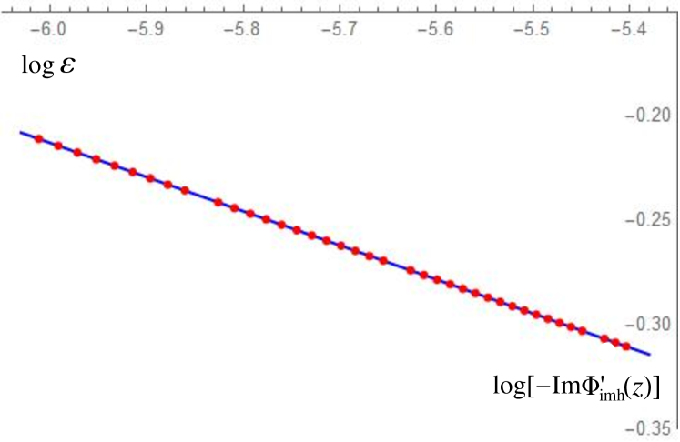
Figure 8: Numerical data points (red dots) for $\log[-\mbox{Im}\Phi_{\textrm{imh}}^{\prime}(Z_{0}+i\epsilon)]$ fitted by Eq. (98).

For the subsequent fits, we used the nonlinear formula obtained from Eqs. (89) and (88), with truncated series (84) and (90) dropping all terms whose contributions into Eq. (93) are of the orders higher than $O\big{[}(z-Z_{0})^{8}\big{]}$. As follows from our estimates, the coefficients $a_{k,l}$ for such terms appear be of the order $10^{-2}$ and smaller. This means that for $|z-Z_{0}|<0.2$ contributions of the discarded terms are expected to be of the order of $10^{-9}$ or less.

For this reason the main nonlinear fit for $\Phi_{\textrm{imh}}(z)$ we used $400$ points (95) with $0<\rho<0.2$, i.e., for which $z\in(\Delta_{1}\cup\Delta_{2})$, as defined in Eq. (96). Subsequently, the accuracy of the fit was tested for all subsets (96) of calculated data points. The Table 2 contains the maximum difference (error) between the value of the fit and a numerical value of $\Phi_{\textrm{imh}}(z)$ calculated with the CTM method,

$$\Sigma_{i}=\max\limits_{z\in\Delta_{i}}|\Phi_{\textrm{imh}}(z)-\Phi_{\textrm{imh}}^{\mbox{\tiny CTM}}(z)|\,.$$ (99)

Table 2: The maximum error between $\Phi_{\textrm{imh}}^{\mbox{\scriptsize trun}}(z)$ and $\Phi_{\textrm{imh}}^{\mbox{\tiny CTM}}(z)$ for the points $z\in\Delta_{i}$.

$i$	1	2	3	4	5	6	7	8	9	10
$\Sigma_{i}$	$1.1\times 10^{-10}$	$4.3\times 10^{-11}$	$1.8\times 10^{-8}$	$3.0\times 10^{-7}$	$1.8\times 10^{-6}$	$1.6\times 10^{-5}$	$1.2\times 10^{-4}$	$6.5\times 10^{-4}$	$3.1\times 10^{-3}$	$1.3\times 10^{-2}$

Since the points $z\in\{\Delta_{1}\cup\Delta_{2}\}$ were used for the fit, it is not surprising that for $i=1,2$ the error is of the order of $10^{-10}$ or less. In fact, it coincides with the accuracy of our numerical calculations of $\Phi_{\textrm{imh}}(z)$. The same accuracy also holds for the location of the singularity

$$Z_{0}=2.4291691718(2).$$ (100)

arising from our final fit. The corresponding position of the singular point $\xi_{0}$ for $G_{\textrm{high}}(\xi)$ is

$$\xi_{0}=0.18935060551(3)\,.$$ (101)

Further, Table 2 shows that for the subsequent sets $z\in\Delta_{i}$, with $i\geq 3$, the accuracy of the fit drops down, which is natural due to an increasing effect of truncation of the series (93). Nevertheless, the value of $Z_{0}$, given in Eq. (100), remains stable, even if points $z\in\Delta_{i}$, with $i\geq 3$, are included in the fit.

Table 3: Coefficients $\hat{g}_{k}$, $\hat{\lambda}_{k}$ and $\hat{\alpha}_{k}$

aka	$\hat{g}_{k}$	$\hat{\lambda}_{k}$	$\hat{\alpha}_{k}$
0	0.0928378351	—	-1.3478038278
1	0.1035665061	0.1720881869	0.0845043112
2	-0.0406336255	-0.0530975348	-0.1988535226
3	-0.1021530341	-0.0432647893	0.1096925182
4	0.0622170621	-0.0060926724	0.0588155481
5	-0.0427391325	0.0015477546	-0.0907062356
6	0.0367166751	-0.0026569648	0.0650203209
7	0.0120039152	-0.0046983681	—
8	-0.0179189367	-0.0050775498	—

The final fit for the coefficients $\hat{g}_{k}$, $\hat{\lambda}_{k}$ and $\hat{\alpha}_{k}$ from Eqs. (84) and (90) is shown in Table 3. Let us notice that the higher coefficients may be correct only up to one or two significant digits due to the series truncation. The lower coefficients should be still correct up to eight or nine digits. It is hard to estimate the number of correct digits in each coefficient, so we left them as they were produced by Mathematica.

Let us comment on this in more detail. We need to use all digits in coefficients in Table 3 to produce accurate values for $\Phi_{\textrm{imh}}(z)$ from the Appendix. Any truncation will cause a significant deviation from the values given there. It seems that this contradicts the statement from the previous paragraph. The explanation is that the series (93) contains too many independent powers in $v$ with a very small separation of exponents. As a result, one can construct another fit for $\Phi_{\textrm{imh}}(z)$ which will reproduce the data from Appendix with $10^{-10}$ accuracy but higher coefficients will coincide only up to one or two significant digits. In other words, one needs the data with much higher precision to get reliable information about coefficients with $k>2$ in Table 3.

Now let us give coefficients $a_{k,l}$ of the series expansions (93) for the function $G_{\text{YL}}(z)$. They are shown in Table 4. The coefficient $b_{0}$ coming from the leading power in the second term of Eq. (92) is estimated as

$$b_{0}=0.0623126407.$$ (102)

Let us notice that to get the series expansion for $\Phi_{\textrm{imh}}(z)$ from $G_{\text{YL}}(z)$ we could use Eq. (75). However, due to the presence of the extra factor $(Z_{0}+v)^{2}$, coefficients for $\Phi_{\textrm{imh}}(z)$ will be in the range $(0.1,0.5)$.

We can also get an estimate for the term $c_{\Xi}\,\beta(z)$ in (92)

$$c_{\Xi}\,\beta(z)=0.01015847+0.0070108\,v$$

$$+0.009344\,v^{2}+0.006279\,v^{3}-0.00058\,v^{4}+\ldots$$ (103)

where $v=z-Z_{0}$. From the third term in Eq. (92) we can estimate $c_{\Xi\Xi}$

$$c_{\Xi\Xi}\approx 7.69\,c_{\Xi}^{2}.$$ (104)

Finally, from the expansion for the fourth term in Eq. (93) we obtain

$$c_{\Xi_{8}}\delta(z)=-0.00064-0.00094\,(z-Z_{0})+\ldots$$ (105)

It appears, that the values in Eqs. (103-105) should be understood only as an order-of-magnitude estimate.

Table 4: Coefficients $a_{k,l}$ of the truncated scaling function $G_{\text{YL}}(z)$ from (93)

	0	1	2	3	4	5
0	0.0928378351	-0.2326384010	0.0729439864	-0.0228716546	0.0071714285	-0.0201278728
1	0.1035665061	0.0598168387	-0.0420846767	0.0205105351	-0.0087246739	-0.0105062255
2	-0.0406336255	0.0502778268	-0.0135928541	0.0012416359	0.0012912732	-0.0151031033
3	-0.1021530341	0.0095546595	-0.0076813505	0.0222269546	-0.0081326053	-0.036304106
4	0.0231406896	0.0184911041	-0.0070095153	-0.0314395832	0.0212048796
5	-0.0183244972	-0.0135214010	0.0173465826	0.0001177947
6	0.0426269803	0.0054321576	-0.0088442156
7	0.0237701200	-0.0002697285
8	0.0032474000

Note that the value of $a_{1,0}$ can also be estimated from Eq. (98)

$$a_{1,0}\approx-\frac{6}{5Z_{0}^{2}\sin(\pi/12)}\exp(-1.204)\approx-0.236,$$ (106)

which is below the more accurate value

$$a_{1,0}=2f_{\text{YL}}C_{\text{YL}}^{2}\hat{\lambda}_{1}^{5/6}=-0.232638\ldots$$ (107)

The discrepancy is mostly caused by the fact that Eq. (98) contains an approximate “fitted” value of the leading coefficient $-1/6$, while in Eq. (93) the related exponent $5/6$ is set to its exact value.

Next, we present a few coefficient functions $G_{k}(u)$ in the expansion of $G_{\textrm{high}}(\xi)$ near $\xi=\pm i\xi_{0}$ in terms of variable $u=\xi^{2}+\xi_{0}^{2}$,

$$G_{\text{YL}}(\xi)=G_{0}(u)+G_{1}(u)u^{\frac{5}{6}}+G_{2}(u)u^{\frac{5}{3}}+G_{3}(u)u^{\frac{5}{2}}+\cdots$$ (108)

$$\begin{array}[]{ll}G_{0}(u)&=0.09284+1.871u+19.8u^{2}-371u^{3}+\ldots\\[2.84544pt] G_{1}(u)&=-2.5947-26.154u-172u^{2}+\ldots\\[2.84544pt] G_{2}(u)&=9.076+171.35u+2091u^{2}+\ldots,\\[2.84544pt] G_{3}(u)&=-31.75-878.7u+\ldots.\end{array}$$ (109)

It is instructive to compare the previous results [11] for the scaling function $G_{\textrm{high}}(\xi)$ [given in Eq. (15) and Table 1] and our new results for the function $G_{\text{YL}}(\xi)$ for purely imaginary values of the argument $\xi=ix$ in the interval $x\in(0,0.2)$. As shown in Fig. 9, the two functions match very well in the intermediate region and deviate from each other towards the ends of the interval.

Finally, note that our results for the leading coefficients of the coupling constant

$$\lambda(z)=\hat{\lambda}_{1}\,v+\hat{\lambda}_{2}\,v^{2}+\ldots=\lambda_{1}\,u+\lambda_{2}\,u^{2}+\ldots$$ (110)

are in excellent agreement with the results of Refs. [9, 10] [the variables $v$ and $u$ are defined in Eqs. (78) and (79)]. Indeed, our values

$$\lambda_{1}=3.10916(2)\,,\qquad\lambda_{2}=37.6(8)\,,$$ (111)

corresponding to $\hat{\lambda}_{1},\hat{\lambda}_{2}$ from Table 3, perfectly match the values $\lambda_{1}=3.089\pm 0.008\,,\ \lambda_{2}=38.4\pm 1.6$, given by Eq. (4.7) of Ref. [10]. Similarly, their values for $f_{0}=0.092746\ldots$ (denoted here as $\hat{g}_{0}$) and for $\hat{\alpha}_{0}=-1.32\pm 0.05$, given in their eqs. (3.10) and (4.8), respectively, match our values presented in Table 3.

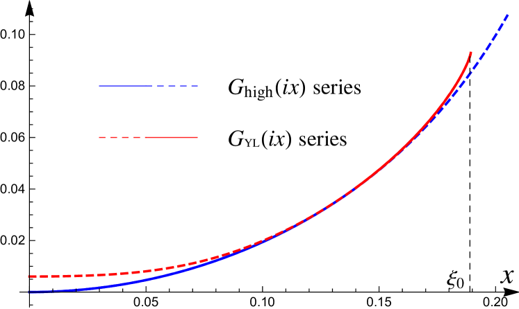
Figure 9: A comparison of $G_{\textrm{high}}(\xi)$ and $G_{\text{YL}}(\xi)$ along the imaginary axis $\xi=ix$

VIII Conclusion

One of the motivations of our work was to confirm and extend the field theory results [9, 10] on the Yang-Lee edge singularity through ab initio calculations, directly from the original lattice formulation (1) of the Ising model.

We used Baxter’s variational approach based on the corner transfer matrix (CTM) method [24], enhanced by an improved iteration scheme [25], known as the corner transfer matrix renormalization group (CTMRG). The main advantage of this approach over other numerical schemes (e.g., the row-to-row transfer matrix method) is that it is formulated directly in the limit of an infinite lattice. Its accuracy depends on the magnitude of truncated eigenvalues of the corner transfer matrix (which is at our control), rather than the size of the lattice. This allows one to calculate the lattice free energy of the model with a rather high precision, of about 30 digits. However, the accuracy of the calculation of the universal characteristics of the continuous scaling theory is limited by the existence of unknown lattice-dependent subleading contribution to the free energy. This is the reason we have chosen the triangular lattice, where such contributions only appear in the order of $\tau^{6}$, where $\tau\sim(T-T_{c})$ is the deviation from the lattice critical temperature. Next, we were able to completely determine these $O(\tau^{6})$ contributions by using the best available perturbation theory calculation of the magnetic susceptibility of the lattice Ising model [8].

In the analysis presented in Sec.III and Sec.IV we used all available exact and perturbation theory results on the 2D lattice Ising model to determine the lattice-dependent regular and subleading contributions to the free energy, as well as to find coefficients entering the nonlinear scaling variables (10) to highest possible orders in the variables $\tau$ and $H$. After these preparations the universal part of the free energy has been numerically calculated using Eq. (22) for a large number of different values of the scaling parameter $\xi$ (or $z$), defined in Eq. (76). The use of the nonlinear scaling variables (10) allowed us to perform calculations sufficiently away from the critical point with a reliable convergence of the algorithm. Using this technique we have numerically calculated (with 10-digit accuracy) the universal scaling function of the Ising Field Theory in the vicinity of the Yang-Lee singularity. This data was used to numerically find a set of main parameters describing the Ising Field Theory as a model of perturbed minimal conformal field theory $M_{2/5}$ involving an infinite tower of irrelevant operators. We also determined the location of the Yang-Lee singularity with a much higher (10 digits) accuracy than it was previously known [10, 26] and confirmed the leading exponent in the singular expansion of the free energy near the critical point predicted by the conformal field theory.

IX Acknowledgments

The authors thank Prof. F. Smirnov for important comments and Prof. A. Zamolodchikov for extremely useful discussions at various stages of our study. V.V.M. acknowledges the support of the Australian Research Council, Grant No. DP190103144.

Appendix: Numerical data for the scaling function

In this Appendix we give numerical values for the function $\Phi_{\textrm{imh}}^{\mbox{\tiny CTM}}(z)$ in the regions $\Delta_{1}$, $\Delta_{2}$ and $\Delta_{3}$ from (96). In our original fitting we used the step $0.002$ for values of $\rho$. Here we only give 50% of all points and use the step $0.004$. The values of $z$ are given by

$$z_{kj}=Z_{0}^{\mbox{\scriptsize in}}+(0.0001+0.004k)e^{\frac{i\pi j}{6}},\quad k=1,\ldots,75,\quad j=0,\ldots,3$$ (S1)

$$Z_{0}^{\mbox{\scriptsize in}}=2.4291691718.$$ (S2)

In Table 5 all points belong to the region $\Delta_{1}\cup\Delta_{2}$. The maximum error for these data is $1.87\times 10^{-10}$. The error is estimated through the calculation of $\Phi_{\textrm{imh}}^{\mbox{\tiny CTM}}(z)$ for several values of $\tau$ as explained after (96). It is slightly higher than the error $\Sigma_{1}$ in the first column of Table 2. In Table 6 we give values for points in $\Delta_{3}$.

Table 5: The values of the function $\Phi_{\textrm{imh}}^{\mbox{\tiny CTM}}(z_{kj})$ for $k=1\ldots,50$ in (S1)

k	j=0	j=1	j=2	j=3
1	0.5381281124	0.5388576178-0.0037551981$\,i$	0.5409580608-0.0069867366$\,i$	0.5441685923-0.0092201138$\,i$
2	0.5316643828	0.5328233012-0.0061499721$\,i$	0.5361791624-0.0115048992$\,i$	0.5413665298-0.0153222565$\,i$
3	0.5260966328	0.5276005678-0.0081648500$\,i$	0.5319740744-0.0153345159$\,i$	0.5387912192-0.0205573761$\,i$
4	0.5210726235	0.5228705683-0.0099492992$\,i$	0.5281177055-0.0187460166$\,i$	0.5363536754-0.0252653491$\,i$
5	0.5164343051	0.5184902651-0.0115704462$\,i$	0.5245091767-0.0218608258$\,i$	0.5340142086-0.0295986922$\,i$
6	0.5120922803	0.5143787623-0.0130662842$\,i$	0.5210914732-0.0247476642$\,i$	0.5317504712-0.0336436922$\,i$
7	0.5079893267	0.5104842833-0.0144611440$\,i$	0.5178281207-0.0274505408$\,i$	0.5295482110-0.0374555959$\,i$
8	0.5040858306	0.5067709856-0.0157718755$\,i$	0.5146938778-0.0299999370$\,i$	0.5273975912-0.0410726638$\,i$
9	0.5003528306	0.5032126646-0.0170108013$\,i$	0.5116702953-0.0324181461$\,i$	0.5252914378-0.0445228788$\,i$
10	0.4967682841	0.4997893762-0.0181873018$\,i$	0.5087433332-0.0347221428$\,i$	0.5232243020-0.0478275482$\,i$
11	0.4933148872	0.4964854624-0.0193087421$\,i$	0.5059019694-0.0369252573$\,i$	0.5211919134-0.0510034067$\,i$
12	0.4899787168	0.4932883244-0.0203810488$\,i$	0.5031373353-0.0390382187$\,i$	0.5191908407-0.0540639260$\,i$
13	0.4867483441	0.4901876190-0.0214090870$\,i$	0.5004421500-0.0410698372$\,i$	0.5172182704-0.0570201703$\,i$
14	0.4836142303	0.4871747133-0.0223969170$\,i$	0.4978103353-0.0430274680$\,i$	0.5152718561-0.0598813788$\,i$
15	0.4805683018	0.4842422993-0.0233479759$\,i$	0.4952367452-0.0449173385$\,i$	0.5133496129-0.0626553764$\,i$
16	0.4776036425	0.4813841164-0.0242652072$\,i$	0.4927169705-0.0467447846$\,i$	0.5114498414-0.0653488693$\,i$
17	0.4747142661	0.4785947448-0.0251511589$\,i$	0.4902471931-0.0485144256$\,i$	0.5095710707-0.0679676661$\,i$
18	0.4718949444	0.4758694503-0.0260080558$\,i$	0.4878240772-0.0502302976$\,i$	0.5077120165-0.0705168428$\,i$
19	0.4691410739	0.4732040640-0.0268378567$\,i$	0.4854446843-0.0518959546$\,i$	0.5058715475-0.0730008712$\,i$
20	0.4664485728	0.4705948890-0.0276422980$\,i$	0.4831064078-0.0535145486$\,i$	0.5040486604-0.0754237191$\,i$
21	0.4638137990	0.4680386259-0.0284229288$\,i$	0.4808069204-0.0550888928$\,i$	0.5022424597-0.0777889290$\,i$
22	0.4612334838	0.4655323133-0.0291811392$\,i$	0.4785441326-0.0566215125$\,i$	0.5004521412-0.0800996825$\,i$
23	0.4587046785	0.4630732792-0.0299181827$\,i$	0.4763161585-0.0581146859$\,i$	0.4986769789-0.0823588509$\,i$
24	0.4562247111	0.4606591018-0.0306351951$\,i$	0.4741212875-0.0595704781$\,i$	0.4969163144-0.0845690386$\,i$
25	0.4537911490	0.4582875763-0.0313332100$\,i$	0.4719579624-0.0609907693$\,i$	0.4951695480-0.0867326173$\,i$
26	0.4514017700	0.4559566876-0.0320131714$\,i$	0.4698247587-0.0623772773$\,i$	0.4934361308-0.0888517558$\,i$
27	0.4490545358	0.4536645878-0.0326759450$\,i$	0.4677203696-0.0637315780$\,i$	0.4917155594-0.0909284440$\,i$
28	0.4467475713	0.4514095759-0.0333223268$\,i$	0.4656435919-0.0650551216$\,i$	0.4900073696-0.0929645144$\,i$
29	0.4444791458	0.4491900821-0.0339530514$\,i$	0.4635933143-0.0663492465$\,i$	0.4883111328-0.0949616591$\,i$
30	0.4422476574	0.4470046528-0.0345687985$\,i$	0.4615685075-0.0676151917$\,i$	0.4866264515-0.0969214452$\,i$
31	0.4400516192	0.4448519390-0.0351701985$\,i$	0.4595682156-0.0688541072$\,i$	0.4849529565-0.0988453284$\,i$
32	0.4378896486	0.4427306853-0.0357578378$\,i$	0.4575915486-0.0700670629$\,i$	0.4832903036-0.1007346635$\,i$
33	0.4357604556	0.4406397209-0.0363322630$\,i$	0.4556376760-0.0712550567$\,i$	0.4816381714-0.1025907149$\,i$
34	0.4336628353	0.4385779517-0.0368939847$\,i$	0.4537058210-0.0724190213$\,i$	0.4799962592-0.1044146650$\,i$
35	0.4315956590	0.4365443522-0.0374434807$\,i$	0.4517952559-0.0735598299$\,i$	0.4783642848-0.1062076215$\,i$
36	0.4295578677	0.4345379609-0.0379811995$\,i$	0.4499052971-0.0746783020$\,i$	0.4767419829-0.1079706247$\,i$
37	0.4275484663	0.4325578734-0.0385075620$\,i$	0.4480353017-0.0757752080$\,i$	0.4751291039-0.1097046528$\,i$
38	0.4255665178	0.4306032380-0.0390229647$\,i$	0.4461846638-0.0768512731$\,i$	0.4735254122-0.1114106278$\,i$
39	0.4236111385	0.4286732516-0.0395277812$\,i$	0.4443528118-0.0779071816$\,i$	0.4719306851-0.1130894193$\,i$
40	0.4216814936	0.4267671553-0.0400223642$\,i$	0.4425392049-0.0789435794$\,i$	0.4703447122-0.1147418496$\,i$
41	0.4197767938	0.4248842310-0.0405070472$\,i$	0.4407433317-0.0799610779$\,i$	0.4687672937-0.1163686968$\,i$
42	0.4178962913	0.4230237988-0.0409821459$\,i$	0.4389647071-0.0809602558$\,i$	0.4671982402-0.1179706984$\,i$
43	0.4160392770	0.4211852132-0.0414479597$\,i$	0.4372028704-0.0819416625$\,i$	0.4656373716-0.1195485544$\,i$
44	0.4142050774	0.4193678617-0.0419047727$\,i$	0.4354573842-0.0829058193$\,i$	0.4640845166-0.1211029299$\,i$
45	0.4123930522	0.4175711612-0.0423528547$\,i$	0.4337278321-0.0838532219$\,i$	0.4625395118-0.1226344578$\,i$
46	0.4106025921	0.4157945570-0.0427924627$\,i$	0.4320138174-0.0847843423$\,i$	0.4610022015-0.1241437408$\,i$
47	0.4088331163	0.4140375204-0.0432238413$\,i$	0.4303149616-0.0856996303$\,i$	0.4594724370-0.1256313534$\,i$
48	0.4070840710	0.4122995468-0.0436472237$\,i$	0.4286309036-0.0865995147$\,i$	0.4579500760-0.1270978444$\,i$
49	0.4053549275	0.4105801545-0.0440628325$\,i$	0.4269612983-0.0874844051$\,i$	0.4564349824-0.1285437377$\,i$
50	0.4036451802	0.4088788829-0.0444708802$\,i$	0.4253058155-0.0883546928$\,i$	0.4549270260-0.1299695344$\,i$

Table 6: The values of the function $\Phi_{\textrm{imh}}^{\mbox{\tiny CTM}}(z_{kj})$ for $k=51,\ldots,75$ $\,i$n (S1)

k	j=0	j=1	j=2	j=3
51	0.4019543458	0.4071952913-0.0448715701$\,i$	0.4236641390-0.0892107524$\,i$	0.4534260817-0.1313757145$\,i$
52	0.4002819614	0.4055289577-0.0452650967$\,i$	0.4220359659-0.0900529422$\,i$	0.4519320294-0.1327627374$\,i$
53	0.3986275835	0.4038794777-0.0456516463$\,i$	0.4204210056-0.0908816059$\,i$	0.4504447541-0.1341310440$\,i$
54	0.3969907869	0.4022464634-0.0460313975$\,i$	0.4188189794-0.0916970728$\,i$	0.4489641450-0.1354810570$\,i$
55	0.3953711632	0.4006295423-0.0464045214$\,i$	0.4172296190-0.0924996591$\,i$	0.4474900954-0.1368131827$\,i$
56	0.3937683205	0.3990283567-0.0467711826$\,i$	0.4156526673-0.0932896684$\,i$	0.4460225027-0.1381278114$\,i$
57	0.3921818820	0.3974425624-0.0471315389$\,i$	0.4140878761-0.0940673926$\,i$	0.4445612681-0.1394253186$\,i$
58	0.3906114851	0.3958718287-0.0474857422$\,i$	0.4125350071-0.0948331124$\,i$	0.4431062961-0.1407060656$\,i$
59	0.3890567810	0.3943158370-0.0478339386$\,i$	0.4109938303-0.0955870981$\,i$	0.4416574949-0.1419704005$\,i$
60	0.3875174339	0.3927742803-0.0481762685$\,i$	0.4094641243-0.0963296098$\,i$	0.4402147755-0.1432186585$\,i$
61	0.3859931199	0.3912468629-0.0485128675$\,i$	0.4079456753-0.0970608982$\,i$	0.4387780522-0.1444511633$\,i$
62	0.3844835269	0.3897332993-0.0488438661$\,i$	0.4064382769-0.0977812052$\,i$	0.4373472419-0.1456682267$\,i$
63	0.3829883536	0.3882333142-0.0491693900$\,i$	0.4049417301-0.0984907641$\,i$	0.4359222643-0.1468701502$\,i$
64	0.3815073092	0.3867466418-0.0494895607$\,i$	0.4034558422-0.0991898001$\,i$	0.4345030418-0.1480572248$\,i$
65	0.3800401129	0.3852730251-0.0498044954$\,i$	0.4019804272-0.0998785308$\,i$	0.4330894990-0.1492297318$\,i$
66	0.3785864931	0.3838122157-0.0501143074$\,i$	0.4005153050-0.1005571663$\,i$	0.4316815631-0.1503879434$\,i$
67	0.3771461874	0.3823639734-0.0504191060$\,i$	0.3990603012-0.1012259101$\,i$	0.4302791634-0.1515321227$\,i$
68	0.3757189420	0.3809280659-0.0507189970$\,i$	0.3976152471-0.1018849586$\,i$	0.4288822313-0.1526625247$\,i$
69	0.3743045108	0.3795042680-0.0510140828$\,i$	0.3961799791-0.1025345023$\,i$	0.4274907001-0.1537793961$\,i$
70	0.3729026561	0.3780923618-0.0513044624$\,i$	0.3947543389-0.1031747255$\,i$	0.4261045053-0.1548829760$\,i$
71	0.3715131472	0.3766921361-0.0515902317$\,i$	0.3933381726-0.1038058068$\,i$	0.4247235841-0.1559734963$\,i$
72	0.3701357607	0.3753033861-0.0518714835$\,i$	0.3919313311-0.1044279190$\,i$	0.4233478755-0.1570511819$\,i$
73	0.3687702797	0.3739259134-0.0521483079$\,i$	0.3905336697-0.1050412301$\,i$	0.4219773200-0.1581162509$\,i$
74	0.3674164943	0.3725595249-0.0524207921$\,i$	0.3891450479-0.1056459029$\,i$	0.4206118602-0.1591689151$\,i$
75	0.3660742004	0.3712040338-0.0526890207$\,i$	0.3877653291-0.1062420951$\,i$	0.4192514396-0.1602093800$\,i$

References

- Onsager [1944] L. Onsager, Phys. Rev. 65, 117 (1944).
- Yang [1952] C. N. Yang, Phys. Rev. 85, 808 (1952).
- McCoy and Wu [1973] B. McCoy and T. T. Wu, The Two-Dimensional Ising Model (Harvard University Press, 1973).
- Baxter [2007a] R. J. Baxter, Exactly Solved Models in Statistical Mechanics (Dover, New York, 2007) pp. xii+498.
- Aharony and Fisher [1983] A. Aharony and M. E. Fisher, Phys. Rev. B 27, 4394 (1983).
- Belavin et al. [1984] A. A. Belavin, A. M. Polyakov, and A. B. Zamolodchikov, Nucl. Phys. B 241, 333 (1984).
- Zamolodchikov [1989a] A. B. Zamolodchikov, Int. J. Mod, Phys. A 4, 4235 (1989a).
- Chan et al. [2011] Y. Chan, A. J. Guttmann, B. G. Nickel, and J. H. H. Perk, J. Stat. Phys. 145, 549 (2011).
- Fonseca and Zamolodchikov [2003] P. Fonseca and A. Zamolodchikov, J. Stat. Phys. 110, 527 (2003).
- Xu and Zamolodchikov [2022] H.-L. Xu and A. Zamolodchikov, J. High Energy Phys. (8), Paper No. 57, 40.
- Mangazeev et al. [2009] V. V. Mangazeev, M. T. Batchelor, V. V. Bazhanov, and M. Y. Dudalev, J. Phys. A 42, 042005, 10 (2009).
- Mangazeev et al. [2010] V. V. Mangazeev, M. Y. Dudalev, V. V. Bazhanov, and M. T. Batchelor, Phys. Rev. E (3) 81, 060103, 4 (2010).
- Newell [1950] G. F. Newell, Physical Review 79, 876 (1950).
- Aharony and Fisher [1980] A. Aharony and M. E. Fisher, Phys. Rev. Lett. 45, 679 (1980).
- Yang and Lee [1952] C. N. Yang and T. D. Lee, Phys. Rev. 87, 404 (1952).
- Lee and Yang [1952] T. D. Lee and C. N. Yang, Phys. Rev. 87, 410 (1952).
- Caselle et al. [2002] M. Caselle, M. Hasenbusch, A. Pelissetto, and E. Vicari, J. Phys. A 35, 4861 (2002).
- Mussardo et al. [2017] G. Mussardo, R. Bonsignori, and A. Trombettoni, J. Phys. A 50, 484003, 52 (2017).
- Cardy [1985] J. L. Cardy, Phys. Rev. Lett. 54, 1354 (1985).
- Cardy and Mussardo [1989] J. L. Cardy and G. Mussardo, Phys. Lett. B 225, 275 (1989).
- Orrick et al. [2001] W. P. Orrick, B. Nickel, A. J. Guttmann, and J. H. H. Perk, J. Stat. Phys. 102, 795 (2001).
- Baxter [1968] R. J. Baxter, Journal of Mathematical Physics 9, 650 (1968), https://doi.org/10.1063/1.1664623 .
- Baxter [1978] R. J. Baxter, J. Statist. Phys. 19, 461 (1978).
- Baxter [2007b] R. J. Baxter, J. Phys. A 40, 12577 (2007b).
- Nishino and Okunishi [1997] T. Nishino and K. Okunishi, Journal of the Physical Society of Japan 66, 3040 (1997).
- Xu and Zamolodchikov [2023] H.-L. Xu and A. Zamolodchikov, Ising field theory in a magnetic field: coupling at (2023), arXiv:2304.07886 [hep-th] .
- Zamolodchikov [1995] A. B. Zamolodchikov, International Journal of Modern Physics A 10, 1125 (1995).
- Smirnov and Zamolodchikov [2017] F. A. Smirnov and A. B. Zamolodchikov, Nucl. Phys. B 915, 363 (2017), arXiv:1608.05499 [hep-th] .