Water Condensation Zones around Main Sequence Stars

Understanding the set of conditions that allow rocky planets to have liquid water on their surface – in the form of lakes, seas or oceans – is a major scientific step to determine the fraction of planets potentially suitable for the emergence and development of life as we know it on Earth. This effort is also necessary to define and refine the so-called ”Habitable Zone” (HZ) in order to guide the search for exoplanets likely to harbor remotely detectable life forms. Until now, most numerical climate studies on this topic have focused on the conditions necessary to maintain oceans, but not to form them in the first place. Here we use the three-dimensional Generic Planetary Climate Model, historically known as the LMD Generic Global Climate Model (GCM), to simulate water-dominated planetary atmospheres around different types of Main-Sequence stars. The simulations are designed to reproduce the conditions of early ocean formation on rocky planets due to the condensation of the primordial water reservoir at the end of the magma ocean phase. We show that the incoming stellar radiation (ISR) required to form oceans by condensation is always drastically lower than that required to vaporize oceans. We introduce a Water Condensation Limit, which lies at significantly lower ISR than the inner edge of the HZ calculated with three-dimensional numerical climate simulations. This difference is due to a behavior change of water clouds, from low-altitude dayside convective clouds to high-altitude nightside stratospheric clouds. Finally, we calculated transit spectra, emission spectra and thermal phase curves of TRAPPIST-1b, c and d with H₂O-rich atmospheres, and compared them to CO₂ atmospheres and bare rock simulations. We show using these observables that JWST has the capability to probe steam atmospheres on low-mass planets, and could possibly test the existence of nightside water clouds.

1 Introduction

Understanding the set of conditions that allow rocky planets to have liquid water on their surface – in the form of lakes, seas or oceans – is a major scientific step to determine the fraction of planets potentially suitable for the emergence and development of life as we know it on Earth. Based on our experience on Earth, liquid water as a solvent is thought to be a necessary (but not sufficient) condition for the existence of life, along with the presence of an energy source and nutrients C,H,N,O,P,S (Forget et al., 2013; Shields et al., 2016). While it is now known to exist in the subsurface of a large sample of planetary bodies (icy moons, Pluto, Triton; see Lunine (2017) and references therein), planets that have liquid water on their surface have two additional favorable properties (Turbet & Selsis, 2023): (1) liquid water is exposed to stellar radiation ; and (2) liquid water is in interaction with the atmosphere, which facilitates the remote search for tracers of life (using the exoplanetary atmosphere to search for biomarkers).

This has motivated numerous theoretical studies to determine the range of parameters (e.g. type of star, incoming stellar radiation) required for a planet to sustain surface liquid water reservoirs, and is the main driver for the definition of the Habitable Zone (HZ) (Kasting et al., 1993; Kopparapu et al., 2013, 2014). The HZ is now a widely used, first-order criterion to determine a zone to search for life-compatible planets, as well as to evaluate the potential habitability of detected planets (see e.g., Borucki et al. 2011).

So far, most numerical climate studies in the field focused on evaluating the conditions needed for a planet to stabilize surface liquid water, whether using one-dimensional (1D) climate models (Kasting et al., 1993; Kopparapu et al., 2013, 2014; Ramirez & Kaltenegger, 2014, 2016; Yang et al., 2016; Ramirez & Kaltenegger, 2017, 2018; Koll & Cronin, 2019; Chaverot et al., 2022) or three-dimensional (3D) Global Climate Models (GCMs) (Wordsworth et al., 2011; Yang et al., 2013; Shields et al., 2013; Yang et al., 2014; Bolmont et al., 2016; Kopparapu et al., 2016; Turbet et al., 2016, 2017; Boutle et al., 2017; Wolf, 2017; Wolf et al., 2017; Kopparapu et al., 2017; Turbet, 2018; Way et al., 2018; Del Genio et al., 2019; Kodama et al., 2019; Yang et al., 2019b, a; Boutle et al., 2020; Wolf et al., 2020; Colose et al., 2021). However, this approach implicitly assumes surface liquid water was available in the first place. This assumption was recently challenged in Turbet et al. (2021) that explored the conditions of surface ocean formation by condensation of the primordial water vapor reservoir. Terrestrial planets are indeed believed to form hot due to their initial accretion energy, and thus to cross a magma ocean stage (Zahnle et al., 1988; Abe, 1997; Hamano et al., 2013; Lebrun et al., 2013; Salvador et al., 2017; Lichtenberg et al., 2023) – where superficial water is present only in the form of vapor – before evolving towards their final state. For liquid water oceans to ever appear on a planetary surface, water initially present in the young and warm planetary atmosphere must be able to condense on the surface in the first place (Hamano et al., 2013; Lebrun et al., 2013; Turbet et al., 2021).

The conditions leading to the condensation of a water ocean after the magma ocean phase have first been studied with 1D numerical climate models (Abe & Matsui, 1988; Hamano et al., 2013; Lebrun et al., 2013; Salvador et al., 2017), which neglect the effects of atmospheric dynamics and clouds. Recently, Turbet et al. (2021) simulated water condensation for the first time in a GCM, specifically for the cases of Earth and Venus, but with potentially far-reaching consequences for a broader range of planets (Kasting & Harman, 2021). They showed that – in water-rich atmospheres – water clouds tend to preferentially form on the nightside and at the poles, owing to the strong subsolar water vapor absorption. Clouds have thus a strong net warming effect that inhibits surface water condensation even at modest insolations, with strong implications for the early habitability of Earth and Venus.

Here we seek to extend the work of Turbet et al. (2021) by extending GCM simulations to the cases of exoplanets, and especially those orbiting stars cooler than the Sun. Terrestrial planets orbiting low-mass, cool, red stars (a.k.a. M-stars) are indeed the best targets we currently have for remote sensing of their atmospheres, and thus to search for tracers of habitability and life (Morley et al., 2017; Kaltenegger, 2017; Lustig-Yaeger et al., 2019; Wunderlich et al., 2019; Fauchez et al., 2019). These planets are thus potentially unique natural laboratories to be able to confront our theories on planetary habitability with observations, in the event that they were able to preserve their atmospheres (Zahnle & Catling, 2017).

2 Method

All the numerical experiments presented in this study are based on the Generic Planetary Climate Model (PCM), which is historically known as the Laboratoire de Météorologie Dynamique (LMD) Generic GCM.

2.1 The Generic PCM

The Generic PCM is a sophisticated 3D Global Climate Model (GCM) that has previously been developed and used to simulate a wide range of exoplanetary atmospheres ranging from that of temperate rocky planets to warm mini-Neptunes (Wordsworth et al., 2011; Leconte et al., 2013b; Charnay et al., 2015a, b; Turbet et al., 2016; Turbet, 2018; Fauchez et al., 2019; Charnay et al., 2021). Specifically, the model has been adapted to simulate water-rich planetary atmospheres (Leconte et al., 2013a) with numerous applications: studying runaway greenhouse on Earth (Leconte et al., 2013a), post-impact atmospheres on Mars (Turbet et al., 2020c), water cloud formation on temperate mini-Neptunes (Charnay et al., 2021), water condensation on early Earth and Venus (Turbet et al., 2021).

We summarize the main features of the model below. The GCM includes a complete radiative transfer that takes into account the absorption and scattering by the atmosphere, the clouds and the surface. The radiative transfer calculations, which are based on the correlated-k approach (Fu & Liou, 1992), use 55 spectral bands in the thermal infrared (from 0.65 to 100$\mu$m ; designed to capture the thermal emission of the planet) and 45 in the visible domain (from 0.3 to 6.5$\mu$m ; designed to capture the incoming stellar radiation). Opacity tables were computed as in Turbet et al. (2021) using the HITRAN 2008 database for wavelength above 1$\mu$m and the HITEMP 2010 database below. We made this choice because most of the differences between HITRAN and HITEMP are below 1$\mu$m (see comparisons done in Goldblatt et al. 2013), and that this significantly reduces the computation time of the opacity tables. The opacity tables also account for the continuum absorptions (from collision-induced absorptions, dimer and far-wings) of N₂-N₂, H₂O-H₂O and H₂O-N₂, using the HITRAN collision-induced absorption (CIA) database (Karman et al., 2019) and the MT$\_$CKD v3.5 database (Mlawer et al., 2012). Subgrid-scale dynamical processes (turbulent mixing and convection) were parameterized as described in Leconte et al. (2013a). Moist convection was taken into account following a moist convective adjustment scheme that originally derives from Manabe & Wetherald (1967) and was later generalized for water-dominated atmospheres in Leconte et al. (2013a). Relative humidity evolves freely and is limited to 100$\%$ (no supersaturation). In practice, when an atmospheric grid cell reaches 100$\%$ saturation and the corresponding atmospheric column has an unstable temperature vertical profile, the moist convective adjustment scheme is performed to get a stable moist adiabatic lapse rate. When condensing, water vapour forms liquid water droplets and/or water ice particles, depending on the atmospheric temperature and pressure, forming clouds. We used a fixed number of activated cloud condensation nuclei (CCNs) per unit mass of air to determine – based on the amount of condensed water – the local, effective radii of H₂O cloud particles (Turbet et al., 2021). The effective radius is then used to compute the radiative properties and the sedimentation velocity of cloud particles. Water precipitation is divided into rainfall and snowfall, depending on the nature of the cloud particles, determined solely by the atmospheric temperature. Rainfall is parameterised to account for the conversion of cloud liquid droplets to raindrops by coalescence with other droplets (Boucher et al., 1995). Rainfall is considered to be instantaneous, that is it goes directly to the surface, but can evaporate while falling through subsaturated layers (Gregory, 1995). In hot and steamy simulations, re-evaporation of precipitation is always complete, that is, precipitation always fully evaporates in the dry lower atmosphere before it reaches the surface. The snowfall rate is calculated using the sedimentation velocity of particles, assumed to be equal to the terminal velocity that we approximate by a Stokes law modified with a ’slip-flow’ correction factor (Rossow, 1978).

The simulations presented in this paper were performed at a spatial resolution of 64 $\times$ 48 in longitude $\times$ latitude. In the vertical direction, the model is composed of 40 distinct atmospheric layers for a 10 bar surface pressure atmosphere, ranging from the surface up to a few Pascals. The exact number of atmospheric layers and model top pressure slightly vary depending on the surface pressure considered. The dynamical time step of the simulations is $\sim$ 15 s, but can slightly vary from one simulation to another. The radiative transfer and the physical parameterisations (such as condensation, convection, etc.) are calculated every 100 and 5 dynamical time steps, respectively.

The main input parameters of our simulations are summarized in Table 1.

Physical parameters	Values
Obliquity (∘)	0
Orbital eccentricity	0
Bare ground albedo	0.2
Ground thermal inertia (J m-2 s-1/2 K-1)	2000
Surface Topography	flat
Surface roughness coefficient (m)	0.01
No. of H2O cloud condensation nuclei (CCN)	105
for ice and liquid (kg-1)

Table 1: Summary of the fixed parameters used in all the new GCM simulations performed in this study.

More details on the model and the parameterizations used in this study can be found in Turbet et al. (2021), and all the references therein. Compared to Turbet et al. (2021), we have proceeded to several changes listed below:

• We varied the type of host star.

• We varied the rotation period, and rotation mode into synchronous rotation. We also fixed the obliquity to 0^∘.

• We varied the values of the masses/radii of planets, depending on the numerical experiments, either to match real planets (in particular, the TRAPPIST-1 inner planets) or to make comparisons with previous studies (in particular, with Yang et al. 2013).

• We varied the internal heat flux. For this, we simply added a constant (through time, and at all latitudes and longitudes) heat flux at the bottom of the model.

These changes are detailed in Tables 5 and 6.

2.2 Strategy of the numerical experiments

Using the Generic PCM, we set up a series of 3D GCM simulations, assuming a N₂+H₂O-rich atmospheric composition, designed to identify the conditions required to trigger water condensation from the atmosphere onto the surface.

For this, we followed a similar strategy than in Turbet et al. (2021). Given a host star (T${}_{\text{eff}}$ between 2600 and 5780 K), we first start with a GCM simulation with partial pressures P${}_{\rm N_{2}}$ = 1 bar and P${}_{\rm H_{2}O}$ = 10 bar (in our baseline scenario), with a high incoming stellar radiation (500 W m^-2 , corresponding to 1.47 the insolation on Earth). P${}_{\rm H_{2}O}$ = 10 bar is much below the possible content of a primordial steam atmosphere (Earth oceans would correspond to $\sim$ 300 bar). Using 10 bar ensures the feasibility of the GCM simulations, and should be sufficient to reach conclusions valid for higher contents, as demonstrated in Section 3.3. For this baseline simulation, we assume an isothermal cloud-free atmospheric temperature profile at 10³ K for the initial state. While the upper atmospheric layers evolve very rapidly towards equilibrium, we used a strategy proposed in Turbet et al. (2021) to converge the deepest layers of the atmosphere, and detailed below. We run the GCM for typically 10 Earth years starting from the initial state described earlier and then we proceed to:

1. run the GCM for 2 Earth years.

2. extrapolate the evolution of the temperature field over $n_{\text{Earth years}}$ (the number of Earth years on which we decide to extrapolate the temperature field) using:

   $$T_{i,j,k}(t+n_{\text{Earth years}})=T_{i,j,k}(t)+n_{\text{Earth years}}\leavevmode\nobreak\ \times\leavevmode\nobreak\ \Delta T_{mean,k},$$ (1)

   with $T_{i,j,k}$ the temperature at the $i$,$j$,$k$ spatial coordinates (corresponding respectively to longitude, latitude and altitude coordinates) and $\Delta T_{mean,k}$ the change of the mean horizontal (averaged over all longitudes and latitudes) temperature field at the altitude layer $k$ calculated over the second Earth year of step 1. $n_{\text{Earth years}}$ was first set arbitrarily to 100, then 50, 20, 10 and eventually 0, when the planetary atmosphere is close to convergence. The transition from one $n_{\text{Earth years}}$ value to another was chosen manually to minimize the convergence time, while avoiding numerical instabilities.

3. repeat the two previous steps, until the top of the atmosphere (TOA) radiative imbalance is lower than $\sim$ 1 W/m². Moreover, we also check that surface temperatures are stable.

We repeated the same procedure for simulations at lower incoming stellar radiations (ISR) until runaway water condensation is reached, except that we used the final equilibrium state of simulations at (previous) higher ISR as the initial state. In comparison to Turbet et al. (2021), the convergence time of the simulations is much longer, in particular for simulations around the coolest stars (TRAPPIST-1 and Proxima Cen). This is due to the fact that for cooler stars, a very small fraction of the stellar flux reaches the low atmosphere and the surface, due to the near-IR absorption by water vapor. For instance, for a GCM simulation of 10 bar of water vapor around TRAPPIST-1 near the water condensation limit, it takes about 150 Earth years of GCM simulations to converge the simulation. This is equivalent to around 2000 Earth years of evolution, taking extrapolation into account. We discuss this aspect in more details in the results section, as it also has an impact on the thermal profiles (Selsis et al., 2023). We note that Turbet et al. (2021) did some sensitivity tests to ensure that the accelerated convergence scheme is working effectively. We thus did not perform any additional test here.

On the whole, and taking advantage of the convergence scheme presented above, we have managed to converge all the simulations presented in this work using a total of 1300 kh CPU on the French supercomputer OCCIGEN. This corresponds to a total of 70 simulations listed in this work, in addition to numerous preliminary and sensitivity simulations (included in the total CPU used and in the carbon budget provided in the Acknowledgments Section).

Finally, we note that for each combination of ISR and star type, we have calculated the rotation period $T$ self consistently with the assumption of synchronous rotation, using the following formula:

$$T\leavevmode\nobreak\ =\leavevmode\nobreak\ 2\pi\leavevmode\nobreak\ \frac{\Bigl{(}d^{2}_{\odot-\oplus}\leavevmode\nobreak\ (\frac{L_{\star}}{L_{\odot}})\leavevmode\nobreak\ (\frac{F_{\oplus}}{F_{p}})\Bigr{)}^{\frac{3}{4}}}{\sqrt{GM_{\star}}}$$ (2)

with $d^{2}_{\odot-\oplus}$ the Sun-Earth distance (in m); $L_{\star}$ and $L_{\odot}$ the stellar and solar luminosity, respectively; $F_{p}$ and $F_{\oplus}$ the stellar flux received at the TOA of the planet and on Earth, respectively; G the gravitational constant (in m³ kg^-1 s^-2); $M_{\star}$ the stellar mass (in kg). The formula is simply a reformulation of Kepler’s third law of planetary motion and assumes that the rotation period is equal to the orbital period (i.e. assumes the synchronous rotation). The luminosity of the star is taken equal to that at the ZAMS (Zero Age Main Sequence), i.e. at the beginning of the Main Sequence Phase (which can be much lower than during the Pre Main Sequence Star, in particular for M stars). This is done because here we are interested in determining the minimal ISR at which a planet has condensed its water reservoir at the start of the Main Sequence Star. This roughly corresponds to the minimum luminosity during the lifetime of stars. For each star type, we used the following mass-luminosity properties:

• For the K5 star, we chose L${}_{\text{K5}}$ = 0.17 L_⊙, M${}_{\text{K5}}$ = 0.7 M_⊙.

• For the M3 star, we chose L${}_{\text{M3}}$ = 1.2 $\times$ 10^-2 L_⊙, M${}_{\text{M3}}$ = 0.31 M_⊙. We used the stellar properties of L98-59 (Kostov et al., 2019).

• For the M5.5 star, we chose L${}_{\text{M5.5}}$ = 1.5 $\times$ 10^-3 L_⊙, M${}_{\text{M5.5}}$ = 0.12 M_⊙. We used the stellar properties of Proxima Centauri (Faria et al., 2022).

• For the M8 star, we chose L${}_{\text{M8}}$ = 5.5 $\times$ 10^-4 L_⊙, M${}_{\text{M8}}$ = 0.09 M_⊙. We used the stellar properties of TRAPPIST-1 (Agol et al., 2021).

2.3 Ensemble of simulations

We set up a grid of GCM simulations (summarized in Tables 5 and 6) designed to explore the conditions of primordial ocean condensation for various types of terrestrial exoplanets, listed below:

• SUN (taken from Turbet et al. 2021), K5, M3, Pcen and T1 are designed to explore surface water condensation on an Earth-like planet (1M_⊕, 1R_⊕) synchronously rotating (except for the Sun case) around its host star. The simulations assume respectively a G2V star (Sun spectrum), a K5 star (4400 K blackbody spectrum), a M3 star (3400 K blackbody spectrum), a M5.5 star (Proxima Cen PHOENIX BT-Settl synthetic spectrum) and a M8 star (TRAPPIST-1 PHOENIX BT-Settl synthetic spectrum). All the simulations assume a H₂O partial pressure of 10 bar, and a N₂ partial pressure of 1 bar.

• M3-YANG is designed to reproduce the same planetary parameters (2 R_⊕, 60 Earth days rotation period) as used in the standard simulations of Yang et al. (2013), except the simulations assume a warm start (1 bar of N₂, 10 bar of H₂O).

• M3-3bar, M3-1bar, M3-0.3bar are designed to explore the impact of water content on the surface water condensation.

• T1b, T1c, T1d, T1e, Pcen-b are designed to explore surface water condensation (and observability) on known exoplanets TRAPPIST-1b, TRAPPIST-1c, TRAPPIST-1d, TRAPPIST-1e and Proxima b, respectively.

• T1b-3bar, T1b-1bar are designed to explore the role of water content on the climate (and observability) of TRAPPIST-1b.

• T1b-Fgeo1, T1b-Fgeo5 and T1b-Fgeo25 are designed to explore the role of internal heat flux on the climate (and observability) of TRAPPIST-1b. The internal heat flux is possibly high on TRAPPIST-1b due to tidal heating (Turbet et al., 2018)

2.4 Computation of observables

Transmission and emission spectra were simulated using the Planetary Spectrum Generator (PSG, Villanueva et al., 2018, 2022). PSG is an online radiative transfer model integrating up-to-date radiative transfer methods and spectroscopic parameterizations, including a realistic treatment of multiple scattering in layer-by-layer spherical geometry. Multiple scattering from aerosols in the atmosphere is computed using the discrete ordinates method, which employs the plane-parallel atmosphere in which the radiation field is approximated by a discrete number of streams angularly distributed. The angular dependence of the aerosol scattering phase function is represented with Legendre polynomials for which the number of expansion terms equal to the number of stream pairs. For each available aerosol type (e.g., Massie & Hervig, 2013), look-up-tables of Legendre expansion coefficients are pre-computed using an assumed particle size distribution. PSG contains billions of spectral lines of thousands of species from several constantly updated spectroscopic repositories such as HITRAN, ExoMol, JPL, CDMS, GSFC-Fluor. In this work, we used the latest HITRAN database (Gordon et al., 2022). The PSG noise model for NIRISS, NIRSpec and MIRI instruments have been benchmarked with the JWST ETC. The PSG noise model was benchmarked with current post JWST launch sensitivities by using the JWST Exposure-Time-Calculator (ETC) version 1.7. We used the NASA JWST website to establish the optics temperature post commissioning ($\sim$ 40K). For each instrument, we computed the unsaturated signal-to-noise ratio (SNR) from the ETC by using the appropriate filter, subarray, readout pattern, group per integration and integrations per exposure. We adjusted the number of exposures, exposure time, readout noise and dark current in PSG to match these numbers. The total background level for the observations (e-/s) was retrieved from the ETC, and we used a consistent background level in PSG. To estimate the effective instrument throughput efficiencies needed by PSG, we compared the extracted flux from the source (e-/sec) in the ETC and we adjusted the throughput parameter in PSG to match these levels. Finally, we checked that the simulated SNR from the ETC matched the ones we computed with PSG for a set of representative cases.

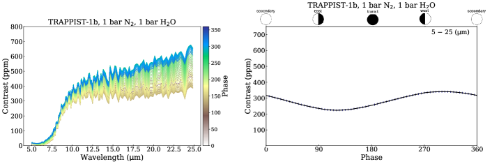
(a)

(b)

(c)

Figure 20: Thermal emission spectra at various phase angles (left). Thermal phase curve (right) integrated over all wavelengths.

To ingest the 3D atmospheric fields (temperature, pressure, volume mixing ratios of molecular species, and mass mixing ratios and particle sizes for liquid and water ice clouds) produced by the Generic PCM and create synthetic spectra, we used the PSG module named GlobES (Global Exoplanetary Spectra, Villanueva et al. 2022). For transmission spectroscopy, GlobES computes the radiative transfer at each GCM latitude chunk across the terminator to create a local spectrum. Each of them are then averaged to create an average terminator spectrum for the planet. For emission spectra, GLobES performs radiative transfer simulations across the whole observable disk, and the individual spectra are integrated considering the projected area of each bin. Because radiative transfer calculations across the full observable disk are very expensive, we have horizontally binned GCM data by a factor of 3, as typically done to speed up the calculation, leading to 3 $\times$ 3 (latitude $\times$ longitude = 9) binning, and a speed up of 9 times while sacrificing a little accuracy. Thermal phase curves have been computed at all phase angles (with a step of 5 degrees) along the orbit. Broadband phase curves have been integrated over the MIRI 5–25 $\mu m$ range (see Fig. 20 to 26). To compare with MIRI observations in photometric bands, we have integrated the high-resolution emission spectra using the spectral transmission function of each MIRI band (for F1280W and F1500W bands, in this work).

3 Results

3.1 Preferential nightside cloud formation and climate multi-stability

Our most striking result is that in all the simulations we did (listed in Tables 5 and 6) water clouds form preferentially on the nightside and at the poles. This is illustrated in Fig. 1 (top row) that shows the column-integrated water cloud distribution for a tidally-locked planet (2 R_⊕, 1.4 g_⊕) around a M3 star, for a fixed rotation period of 60 Earth days, and for various ISR (’M3-YANG’ cases in Table 6). The parameters used here for the star and the planet closely match those used in the standard simulations of Yang et al. (2013), except that it is assumed here that the entire water reservoir is initially vaporized in the atmosphere. While ’cold start’ GCM simulations in Yang et al. (2013) – with a global surface liquid water ocean – predict the formation of low-altitude, convective dayside clouds, our ’hot start’ GCM simulations – with a steam atmosphere and a dry surface – predict the formation of high-altitude, stratospheric nightside clouds.

Fig. 2b shows the horizontal distribution of clouds and winds in the tidally-locked (TL) coordinates (Koll & Abbot, 2015). In the TL coordinate system, the TL latitude is equal to 90^∘ at the substellar point and -90^∘ at the antisubstellar point. Fig. 2b was derived by converting Fig. 2a (which is similar to Fig. 1, top row, right column) using the python package of Koll (2020). The TL coordinates highlight well the strong dichotomy in cloud distribution between the dayside and the nightside of the planet, with two maxima located near the two wind gyre structures (near -120^∘ in longitude, $\pm$60^∘ in latitude).

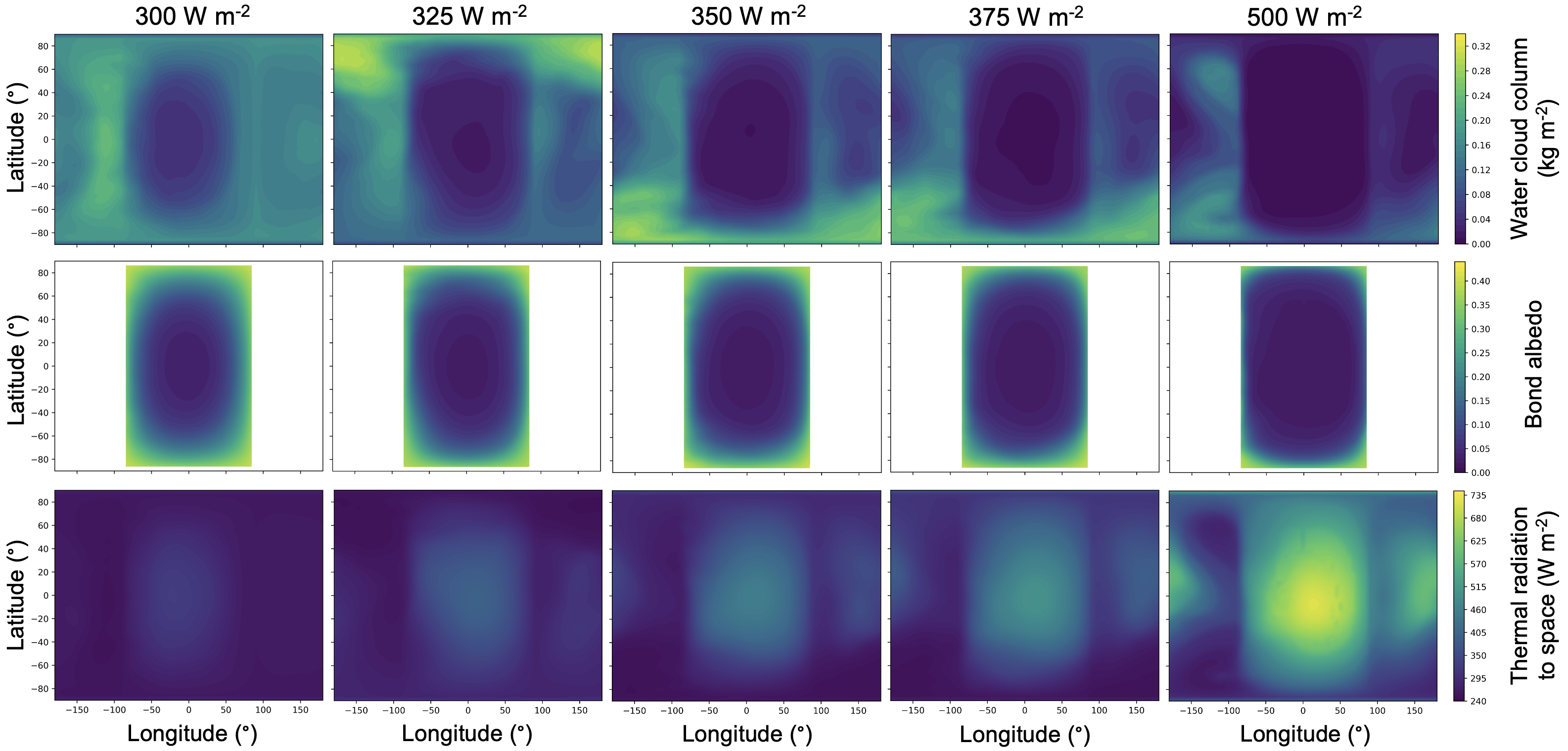
Figure 1: Water cloud column (top), albedo (middle) and thermal emission to space (bottom) horizontal maps, for an initially hot and steamy 2 R_⊕ planet (with a 10 bar of H₂O + 1 bar of N₂ atmosphere) synchronously rotating (fixed rotation period of 60 Earth days) around a M3 star. The simulations shown here were forced to ISR (defined here and throughout the manuscript as the global mean average value, i.e. a factor of 4 lower than the stellar flux at the substellar point) ranging from 500 W m^-2 or 1.47 F_⊕ (right) down to 300 W m^-2 or 0.88 F_⊕ (left), and the outputs were averaged over 250 Earth days. The associated simulations names are M3-YANG-1, 2, 3, 4 and 5. For reference, insolation is 340.5 W m^-2 on present-day Earth.

The cloud formation mechanism at play has already been identified and discussed for the cases of early Earth and Venus in Turbet et al. (2021), and we find that the same mechanism also applies here to tidally-locked exoplanets. In short, water vapor which is the main component of the atmosphere efficiently absorbs the incident stellar flux. This shortwave heating breaks moist convection on the dayside and thus prevents the formation of convective clouds. This shortwave heating also drives strong winds in the stratosphere that transport air parcels from the dayside to the nightside, which is qualitatively similar to the results of Fujii et al. (2017). As the air parcels move to the nightside, they are cooled by longwave emission (i.e., thermal emission to space) which reduces their temperature down to the saturation temperature of water vapor. This leads to large-scale condensation, and thus to the formation of stratospheric clouds preferentially located on the nightside and at the poles. The 3D distribution of water clouds and winds is depicted in Fig. 2bc using the TL coordinates. We note that we observe in Fig. 2abc a slight decrease of the cloud cover at the antisubstellar point. This is particularly visible in the TL coordinates, with a decrease of clouds between -60^∘ and -90^∘ TL latitudes. This reduction in cloud content is associated with a downward movement of air parcels near the antisubstellar point (see the wind field in Fig. 2c). This subsidence produces adiabatic warming thus reducing the amount of clouds in this region, which is qualitatively similar to the results of Charnay et al. (2021). We also note that the asymmetry between North and South hemispheres in the cloud distribution (see e.g., Fig. 2a) is due to temporal variability. The asymmetry in fact vanishes when averaging over a longer period of time (e.g. 5 Earth years, instead of 250 Earth days, as illustrated in Fig. 4).

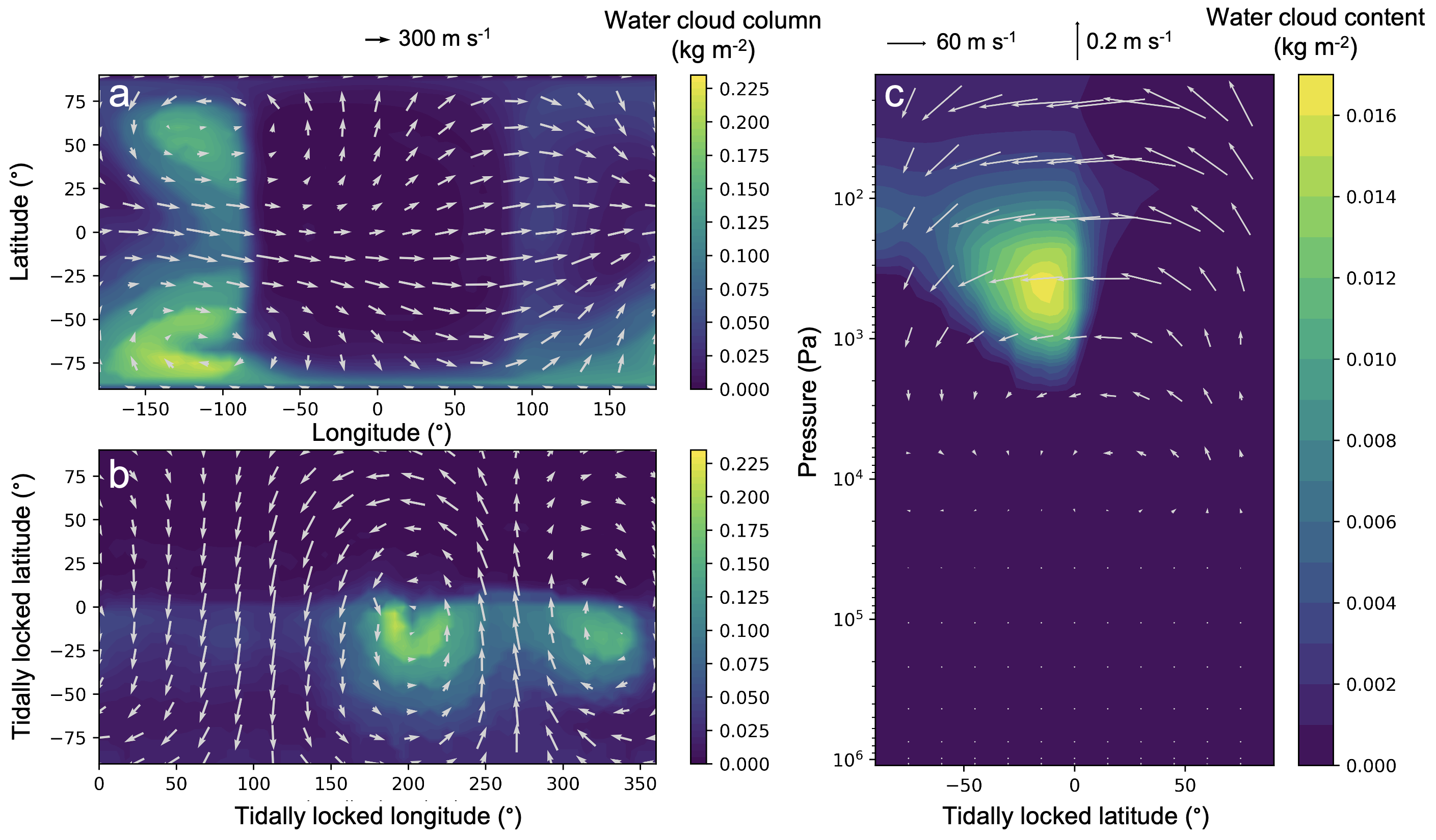
Figure 2: Water cloud horizontal and vertical distributions. Water cloud column (a) in latitude vs longitude coordinates and (b) tidally-locked coordinates (b). Water cloud content vertical distribution (c) as a function of tidally-locked latitude (averaged over all tidally-locked longitudes). The plots were computed for an initially hot and steamy 2 R_⊕ planet (with a 10 bar of H₂O + 1 bar of N₂ atmosphere) synchronously rotating (fixed rotation period of 60 Earth days) around a M3 star, and forced to an ISR of 500 W m^-2 (simulation M3-YANG-1). The outputs were averaged over 250 Earth days. For reference, insolation is 340.5 W m^-2 on present-day Earth. Wind fields are superimposed on the plots. Winds are plotted at a pressure of $\sim$ 50 Pa in panels a and b, and averaged over all tidally-locked (TL) longitudes in panel c.

The preferential accumulation of clouds on the nightside and lack of clouds on the dayside has two consequences: (1) lowering the bond albedo (see Fig. 1, middle row); and (2) producing a strong greenhouse effect on the nightside (see Fig. 1, bottom row). Fig. 1 (bottom row) illustrates that the planetary thermal radiation displays a strong day-to-night amplitude. This is first due to the greenhouse effect of nightside clouds ; and second, this is due to the fact that a significant fraction of the ISR is absorbed high in the atmosphere, which is qualitatively similar to the results of Wolf et al. (2019). This shortwave heating heats up the atmosphere on the dayside, which thermally re-radiates to space, further increasing the day-night Outgoing Thermal Radiation (OTR) contrast. This 3D effect is the direct consequence of the distribution of the stellar flux, combined with the strong, direct absorption of this flux by water vapor.

As a consequence, we find the same result than in Turbet et al. (2021), that depending on the initial state (all water initially in the form of vapor in the atmosphere ; versus all water initially condensed at the surface), there is a wide range of ISR for which climate end states are different. This hysteresis is illustrated in Fig. 3 for the surface temperature (Fig. 3a), planetary albedo (Fig. 3c), upper atmosphere water vapor mixing ratio (Fig. 3b) and greenhouse effect ((Fig. 3d). The greenhouse effect G is defined as the difference between the surface temperature and the equilibrium temperature of the planet:

$$G\leavevmode\nobreak\ =\leavevmode\nobreak\ T_{\text{surf}}-\Bigl{(}\frac{OTR}{\sigma}\Bigr{)}^{\frac{1}{4}}$$ (3)

with T${}_{\text{surf}}$ the global mean surface temperature, OTR the global mean thermal radiation to space and $\sigma$ the Stefan–Boltzmann constant. Our new simulations (Fig. 3, red branches) are compared to that of the standard simulations of Yang et al. (2013) (Fig. 3, blue branches) in the standard case of a 2 R_⊕, 1.4 g_⊕ planet synchronously rotating (fixed rotation period of 60 Earth days) around a M3 star.

Fig. 3a shows the evolution of the surface temperature as a function of ISR, for two types of initial states. The arrows indicate an estimate of the ISR threshold limit at which the radiative TOA budget becomes unstable, leading to a runaway greenhouse (for the ’cold start’ sequence) and a runaway water condensation (for the ’hot start’ sequence). For the hot start sequence, the arrows are positioned halfway between the last simulation (or lowest ISR) that does not lead to surface water condensation and the first simulation (or higher ISR) that does lead to surface water condensation (i.e., the simulation for which rainwater hits the surface). For the cold start sequence, the arrows are positioned halfway between the last simulation (or highest ISR) that avoid runaway greenhouse and the first simulation (or lowest ISR) that goes into runaway greenhouse (Yang et al., 2013). As already identified in Turbet et al. (2021), near the water condensation limit the amount of dayside clouds grows when reducing the ISR, leading to an increase in bond albedo (see Fig. 3c, red branch). As soon as the water condensation limit is attained, the dayside becomes largely covered by clouds, which makes the bond albedo jump. This produces a strong TOA radiative desequilibrium, which inevitably leads to the condensation of water vapor on the surface. This imbalance is maintained until almost all the water reservoir has condensed onto the surface. This cloud-driven positive feedback is what triggers the runaway water condensation.

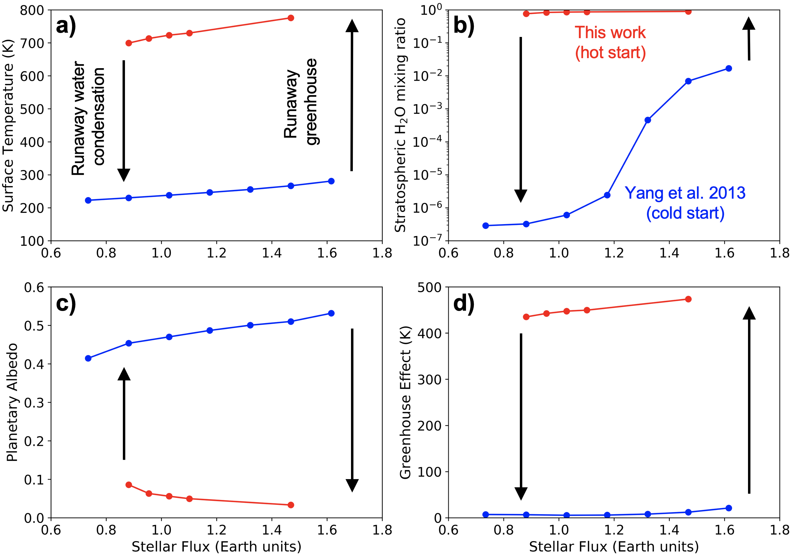
Figure 3: Hysteresis loops and conditions of ocean formation for an initially hot and steamy 2 R_⊕ planet (with a 10 bar of H₂O + 1 bar of N₂ atmosphere) synchronously rotating (fixed rotation period of 60 Earth days) around a M3 star (simulation M3-YANG-1). The figure depicts the evolution of surface temperature (top left), stratospheric water mixing ratio (top right), bond albedo (bottom left) and greenhouse effect (bottom right) as a function of the incoming stellar flux. The blue branches correspond to simulation results (Yang et al., 2013) that assume water is initially condensed on the surface. The red branches (this study) correspond to initially hot and steamy simulation results, that assume water is initially in vapor form in the atmosphere.

3.2 Water condensation around different types of stars

We conducted a grid of simulations to explore the conditions for water condensation depending on the type of host star (from Sun-like stars to late M stars ; see cases ’SUN’, ’K5’, ’M3’, ’Pcen’ and ’T1’ in Table 5), for an Earth-like planet (1M_⊕, 1R_⊕) synchronously rotating (except for the Sun case) around its host star. Again, we find that in all the simulations, water clouds preferentially form on the nightside and at the poles. This is illustrated in Fig. 4 (top row) that shows the column-integrated water cloud distribution for the planet depending on the type of host star. Here again, the albedo (Fig. 4, middle row) and the OTR (Fig. 4, bottom row) maps are correlated and anti-correlated with the distribution of clouds, respectively.

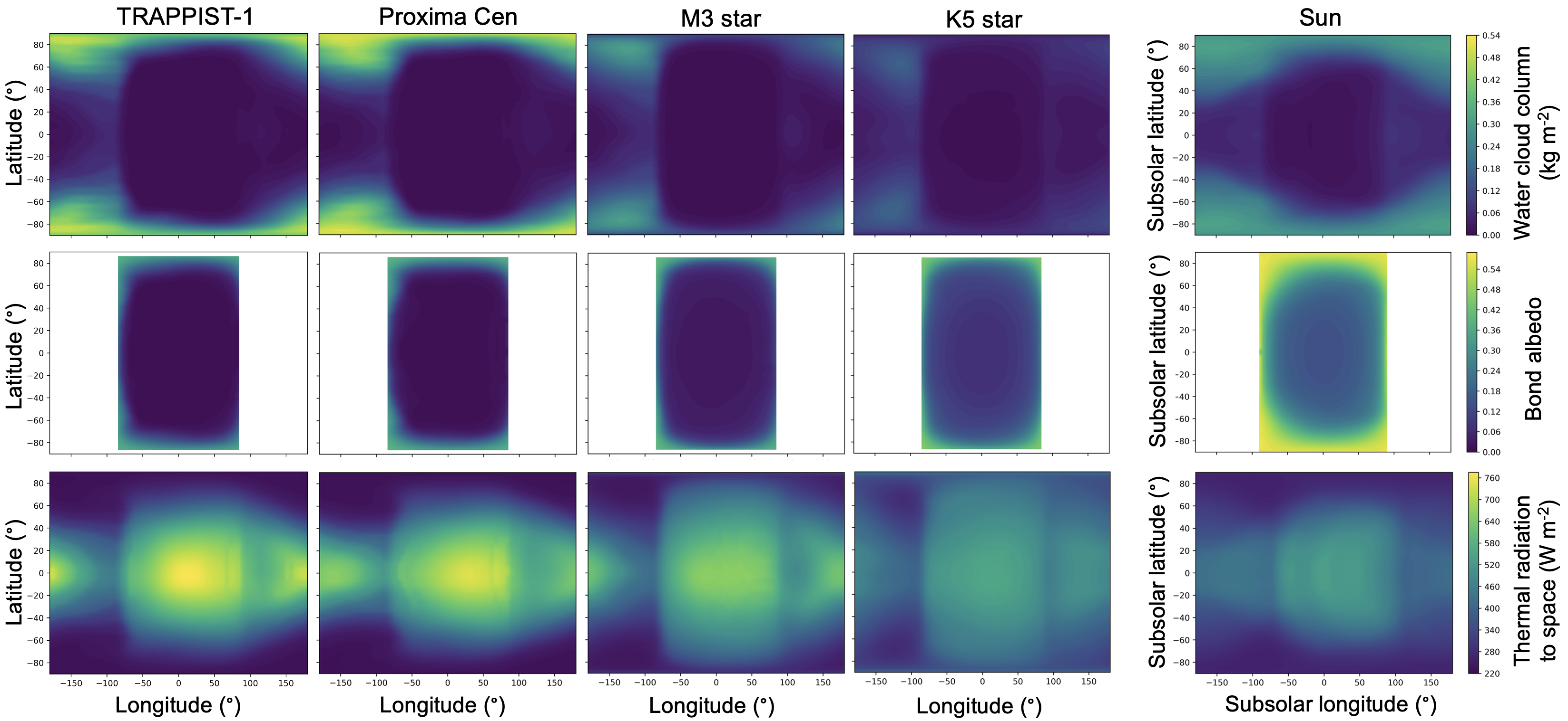
Figure 4: Water cloud column (top), albedo (middle) and thermal emission to space (bottom) horizontal maps, for an initially hot and steamy 1 R_⊕ planet (with a 10 bar of H₂O + 1 bar of N₂ atmosphere) orbiting around different types of stars: TRAPPIST-1 (T_⋆ $\sim$ 2600 K), Proxima Centauri (T_⋆ $\sim$ 3050 K), a M3 star (T_⋆ $\sim$ 3400 K), a K5 star (T_⋆ $\sim$ 4400 K) and the Sun (T_⋆ $\sim$ 5780 K). The associated simulations names are T1-1, Pcen-1, M3-1, K5-1 and SUN-1, respectively. The simulations shown here were forced to an ISR of 500 W m^-2 (i.e. 1.47 F_⊕), and the outputs were averaged over 100 Earth days. We made the assumption of a synchronous rotation for all the simulations, except for those of the Sun (where we took the results directly from Turbet et al. (2021) in which rotation period is equal to 1 Earth day, orbital period is equal to 365 Earth days, and obliquity is equal to 23.5^∘). For this simulation only, the maps were calculated in the heliocentric frame (that is, keeping the subsolar point at 0^∘ longitude and 0^∘ latitude), and using an average of five Earth years as in Turbet et al. (2021).

As discussed in the previous section, we observe again a slight decrease of the cloud cover at the antisubstellar point (Fig. 4, top row), associated with subsidence warming. We note that the cloud patterns are broadly similar between all types of host star, in particular all those assuming a synchronous rotation. The cloud content is maximum near the two wind gyre structures – the coldest parts of the atmospheres – in all simulations, although their exact location and extension is affected by the parameters of the simulations (in particular, the rotation rate ; see Carone et al. 2014, 2015, 2016).

While the thermal emission maps (Fig. 4, bottom row) are qualitatively similar between all simulations, we observe a much higher dayside emission for the lowest mass stars (TRAPPIST-1, Proxima Cen) than the other cases. This is first due to the bond albedo being lower (see Fig. 4, middle row ; see also discussions below), but also, and above all, to the fact that low-mass stars emit more near-IR flux which gets absorbed higher up in the atmosphere (Fujii et al., 2017) and directly re-emitted to space on the dayside (Wolf et al., 2019).

Figure 5: Conditions of ocean formation for initially hot and steamy 1 R_⊕ planets (with a 10 bar of H₂O + 1 bar of N₂ atmosphere) orbiting around different types of stars: TRAPPIST-1 (T_⋆ $\sim$ 2600 K), Proxima Centauri (T_⋆ $\sim$ 3050 K), a M3 star (T_⋆ $\sim$ 3400 K), a K5 star (T_⋆ $\sim$ 4400 K) and the Sun (T_⋆ $\sim$ 5780 K). The associated simulations names are T1-1 to 8, Pcen-1 to 7, M3-1 to 7, K5-1 to 6 and SUN-1 to 6, respectively. The figure depicts the evolution of surface temperature (top) and bond albedo (bottom) as a function of the incoming stellar flux. We made the assumption of a synchronous rotation for all the simulations, except for those of the Sun (where we took the results directly from Turbet et al. (2021) in which rotation period is equal to 1 Earth day, orbital period is equal to 365 Earth days, and obliquity is equal to 23.5^∘). Horizontal dashed lines indicate the bond albedos of planets in runaway greenhouse, obtained from 1D cloud-free calculations (Kopparapu et al., 2013). The dashed arrows indicate the ISR threshold limit at which the radiative TOA budget becomes imbalanced, leading to a runaway water condensation.

For each type of stars, we used the GCM simulations to build their water condensation sequences, illustrated in Fig. 5. Fig. 5a shows the evolution of the surface temperature as a function of ISR, for all the types of host stars. The dashed arrows indicate the ISR threshold limit at which the radiative TOA budget becomes imbalanced, leading to a runaway water condensation.

There are several noticeable points in this Fig. 5:

1. Firstly, we notice that the surface temperatures are lower for cooler stars despite that more ISR is absorbed by the planet (as illustrated in Fig. 5b showing the bond albedos). This is somewhat counter-intuitive, as cooler stars have been shown to produce consistently warmer climates on planets with Earth-like atmospheres (Kopparapu et al., 2013; Shields et al., 2013; Godolt et al., 2015; Wolf et al., 2019). We discuss this effect in more details below.

2. Secondly, the bond albedo decreases for cooler stars, which was expected (see e.g., Kopparapu et al. 2013; Shields et al. 2013). Moreover, the bond albedo increases when the ISR decreases. This effect, which is discussed in Section 3.1, is what drives the sharp radiative budget deficit at the TOA, and thus what defines the runaway water condensation for all types of stars. Finally, as the ISR reaches the highest values we have explored, Fig. 5b shows that the bond albedos seem to converge asymptotically towards the results from 1D cloud-free calculations (here taken from Kopparapu et al. 2013). This is due to the fact that the dayside of the planet is getting warmer and therefore has fewer clouds.

3. Thirdly, the water condensation limit ISR threshold decreases in a monotonic way when decreasing the stellar effective temperature. In other words, this indicates that for a given ISR, water condensation is more difficult to attain for planets around M stars than around Sun-like stars. Implications are discussed in Section 3.4.

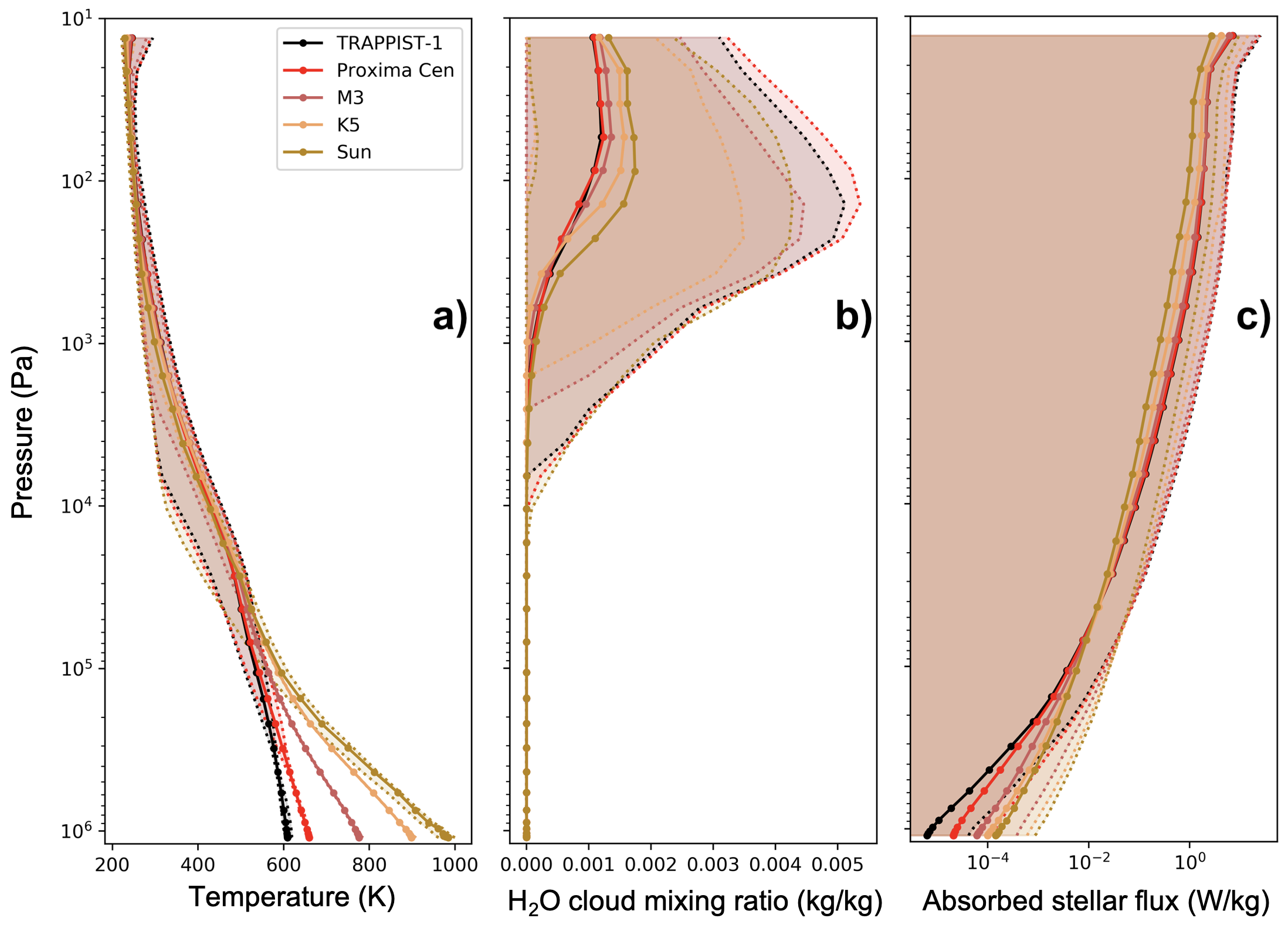
Figure 6: Vertical profiles (global mean, with an envelope defined by global maximum and minimum values) of atmospheric temperatures (left), water cloud mixing ratio (middle) and absorbed stellar fluxes (right). The profiles were computed for an initially hot and steamy 1 R_⊕ planet (with a 10 bar of H₂O + 1 bar of N₂ atmosphere) orbiting around different types of stars: TRAPPIST-1 (T_⋆ $\sim$ 2600 K), Proxima Centauri (T_⋆ $\sim$ 3050 K), a M3 star (T_⋆ $\sim$ 3400 K), a K5 star (T_⋆ $\sim$ 4400 K) and the Sun (T_⋆ $\sim$ 5780 K). The curves were drawn from the same GCM simulations as in Fig. 4. The associated simulations names are T1-1, Pcen-1, M3-1, K5-1 and SUN-1, respectively.

To understand in more details why surface temperatures decrease (in thick H₂O-rich atmospheres) for cooler stars, we show in Fig. 6abc vertical profiles of the atmospheric temperatures, cloud mixing ratios and absorbed stellar flux. While atmospheric temperatures are higher for cooler stars in the upper atmosphere (in the stratosphere, typically above 10⁴ Pa), this is reversed below in the troposphere where atmospheric temperatures become lower for cooler stars. Following Selsis et al. (2023), we found that the absorption of the ISR by water bands – combined with Rayleigh scattering of H₂O molecules – is so efficient, that not enough shortwave flux reaches the lower atmosphere to sustain convection. This is illustrated in Fig. 6c, which shows indeed that the absorbed stellar radiation drops in the low atmosphere due to most of the flux being absorbed higher in the atmosphere. Selsis et al. (2023) explored and discussed this effect in details, and we verify here that the same effect appear in all our GCM simulations of thick H₂O-rich atmospheres. The clouds have little effect on the temperature structure in the low atmosphere, given that the dayside is almost entirely depleted in clouds (Fig. 4, top row). In other words, from the point of view of the shortwave radiative transfer calculations, the atmosphere behaves closely to the cloud-free case thus validating the approach of Selsis et al. (2023).

3.3 Impact of the water content

We conducted a series of simulations to explore the effect of the water mass fraction in our simulations (M3 from Table 5 and M3-3bar, M3-1bar, M3-0.3bar from Table 6), and how it may potentially affect the water condensation limit. Fig. 7 shows the water condensation sequences for H₂O atmospheric pressures from 0.3 to 10 bar (all simulations assume 1 bar of N₂ as a background gas).

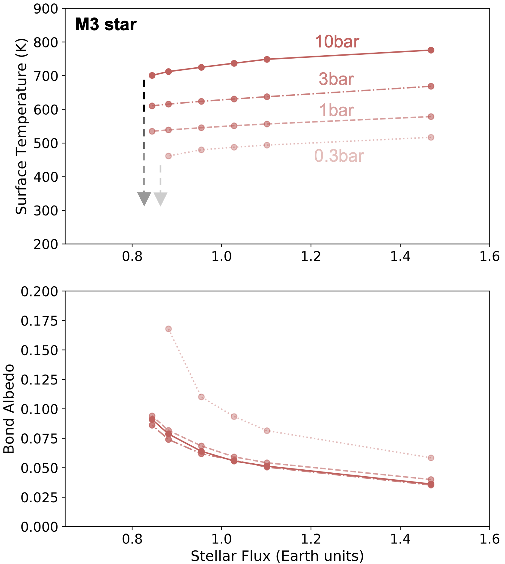
Figure 7: Conditions of ocean formation for initially hot and steamy 1 R_⊕ planets synchronously rotating around a M3 star (T_⋆ $\sim$ 3400 K). The figure depicts the evolution of surface temperature (top) and bond albedo (bottom) as a function of the incoming stellar flux, for four different bulk atmospheric compositions: 10 bar of H₂O + 1 bar of N₂ (M3), 3 bar of H₂O + 1 bar of N₂ (M3-3bar), 1 bar of H₂O + 1 bar of N₂ (M3-1bar) and 0.3 bar of H₂O + 1 bar of N₂ (M3-0.3bar).

We first notice that the surface temperatures increase with water content, as already seen in Turbet et al. (2021), and as expected from the increasing greenhouse effect of water vapor. Note however that for planets orbiting very cool stars, the surface temperature increases very little with H₂O partial pressure, because the stellar flux in the lower atmosphere is too low to maintain convection and thus the thermal profile reaches an isotherm (see Section 3.5 where this is discussed in the context of TRAPPIST-1b).

The bond albedo sequence looks very similar for all H₂O partial pressures explored, except the one at P${}_{\rm H_{2}O}$ = 0.3 bar. For this case, the water vapor content is low enough to reduce the fraction of ISR absorbed by the atmosphere, which leads to an increase in bond albedo (as a reminder, the surface albedo is fixed at 0.2 in these simulations). A similar behavior is seen in the 1D cloud-free simulations of Kopparapu et al. (2013) (see e.g., their Fig. 6a) where the bond albedo for an Earth-like planet around a M-type star decreases as surface temperature increases, due to the increasing water vapor content. Moreover, given that less ISR is absorbed on the dayside by water vapor, the dayside cloud positive feedback (producing the runaway water condensation introduced in previous subsections) is even more efficient. This is visible in Fig. 7b revealing that the bond albedo increases more rapidly for the P${}_{\rm H_{2}O}$ = 0.3 bar simulation when decreasing ISR. As a result, the water condensation limit occurs at slightly higher ISR for the P${}_{\rm H_{2}O}$ = 0.3 bar simulation (see Fig. 7a) than for the other H₂O partial pressures explored. It is not clear if this trend would remain for even lower H₂O atmospheric mixing ratios and/or H₂O partial pressures, given that the saturation temperature also decreases with partial pressure. This deserves to be explored in more details, with possibly some interesting implications for the case of early Venus, and more generally for the case of land exoplanets (Kodama et al., 2015; Ding & Wordsworth, 2020).

The fact that the evolutions of the bond albedo as a function of ISR (see Fig. 7b) look very similar for all GCM simulations with P${}_{\rm H_{2}O}$ $\geq$ 1 bar is a good indication that we are capturing well here the climate regime in which H₂O is a dominant gas (starting from P${}_{\rm H_{2}O}$ = 1 bar, up to pressures as high as desired). Although the amount of water has an impact on the surface temperature (see Fig. 7a), for planets more irradiated than the water condensation limit the surface temperatures are always higher than that of the saturation temperature of the assumed H₂O partial pressure. The fact that the P${}_{\rm H_{2}O}$ = 10 bar simulation produces surface temperatures even higher than the critical temperature of water (T${}_{\text{crit}}$ = 647 K) indicates that for P${}_{\rm H_{2}O}$ $\geq$ 10 bar, the water condensation limit would remain unchanged. More specifically, H₂O-rich atmospheric simulations at different total pressures have thermal profiles that overlap well (see Fig. 13c, in the context of TRAPPIST-1b). Increasing the surface pressure to higher values would likely produce an extension of the thermal profile, while keeping a similar profile at low atmospheric pressures.

For planets orbiting ultra-cool stars, Selsis et al. (2023) showed that the thermal profile in the lower atmosphere can converge to an isotherm at a temperature that is lower than that of the critical point of water, potentially permitting the co-existence of a steam atmosphere and liquid water oceans for planets more irradiated than the runaway greenhouse limit. Although we did not explore this possibility in detail, our simulations for TRAPPIST-1 inner planets (see Figs. 12 and 13) support this result. This result might however be restricted to a purely theoretical experiment, since a tiny internal heat flux is enough to increase the surface temperatures above the critical temperature of water (Selsis et al. 2023 ; see also Fig. 13b in the context of TRAPPIST-1b).

To summarize, the sensitivity experiment described in this subsection shows that the choice of P${}_{\rm H_{2}O}$ = 10 bar for our GCM calculations is a relevant choice to represent all the cases where water is a major component of the atmosphere. Additional radiative active gases (e.g. CO₂) could change the TOA radiative budget, likely producing more warming (see Turbet et al. 2021), but this deserves to be explored quantitatively (see discussions in Section 4).

3.4 Consequences for the Habitable Zone

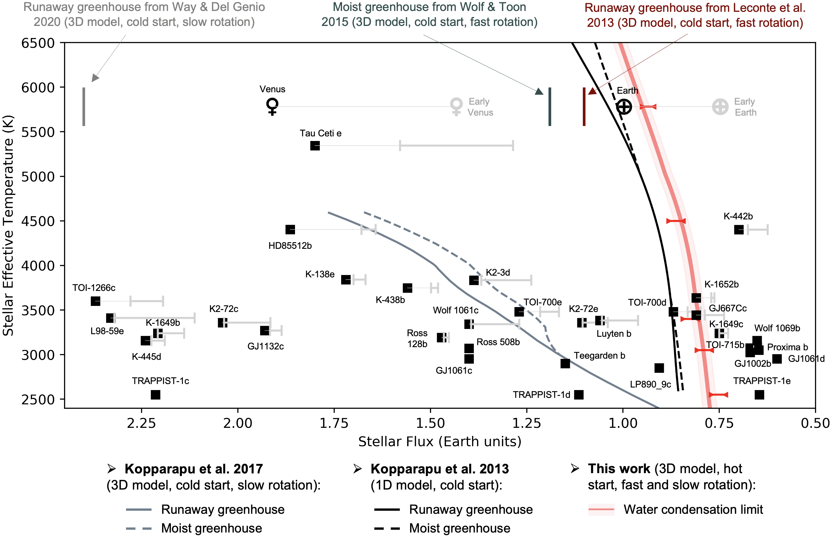
Figure 8: Various inner edge boundaries of the Habitable Zone (HZ) for different types of stars, based on the results of 1D calculations (Kopparapu et al., 2013) and 3D calculations for slow (Kopparapu et al., 2017; Way & Del Genio, 2020) and fast rotators (Leconte et al., 2013a; Wolf & Toon, 2015). The black solid and dashed lines were calculated based on 1D climate calculations, for the runaway greenhouse and the moist greenhouse, respectively (Kopparapu et al., 2013). The grey solid and dashed lines were calculated based on 3D climate calculations of tidally-locked planets, for the runaway greenhouse and the moist greenhouse, respectively (Kopparapu et al., 2017). The red bold line (and red brackets) indicates the newly calculated water condensation limit. All the currently known planets and exoplanets (with a mass $\leq$ 5 M_⊕ and/or a radius $\leq$ 1.6 R_⊕) in or near the inner boundary of the HZ are shown (black squares). We also added (grey brackets) the incoming stellar radiation (ISR) they received at the ZAMS (Zero Age Main Sequence) based on their age estimates, using the grid of stellar models of Baraffe et al. (2015). The water condensation limit (red bold line) should be compared with the ISR that planets received at the ZAMS (grey brackets).

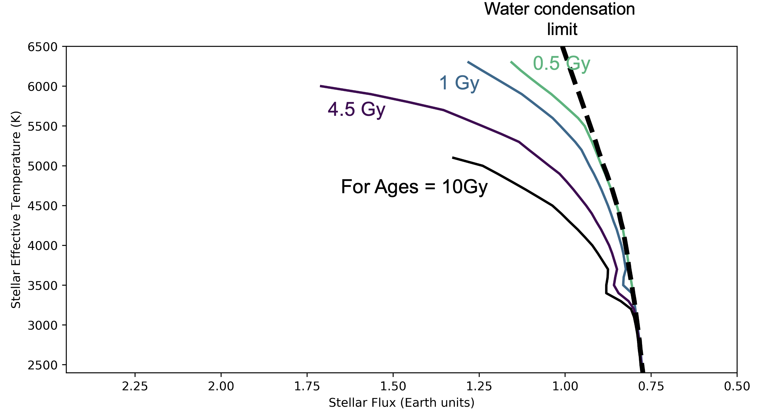
Figure 9: Various positions of the water condensation limit, depending on the age of the planetary system considered. The standard water condensation limit (black dashed line) is valid at the Zero Age Main Sequence (ZAMS). It can be used as is to evaluate the condensation of water on a planet, provided that the insolation of the planet is taken at the ZAMS (see e.g., grey brackets in Fig 8). The other water condensation limits (solid colored lines) indicate, for a planet of age X (with X = 0.5, 1, 4.5, and 10 Gyr here), that if that planet is to the left of the age X curve, then it has never been able to, or will never be able to, condense its water at the surface. These curves were calculated from the standard water condensation curve (black dashed line), and shifted using the grid of stellar models of Baraffe et al. (2015). Numerical values of all the curves are provided in Table 2.

We synthesized our results to define a Water Condensation Zone (WCZ) which we propose to use to redefine the inner boundary of the Habitable Zone (HZ). We remind that the ISR at which the surface water condensation starts is necessarily less than or equal to the ISR required to trigger the runaway greenhouse. It is therefore a more restrictive criterion. Fig. 8 highlights in bold red the water condensation limit calculated with GCM simulations for five types of host stars (Sun-like, K5, M3, M5.5, M8 stars). Planets receiving lower ISR than this limit are within the WCZ of their host star, meaning ocean formation by condensation is permitted. To put this result in context, we have added various inner edge boundaries of the HZ, based on the results of 1D calculations (Kopparapu et al., 2013) and 3D calculations for slow (Kopparapu et al., 2017; Way & Del Genio, 2020) and fast rotators (Leconte et al., 2013a; Wolf & Toon, 2015). We note that the inner edge of the HZ is at much higher ISR for slowly rotating planets, because GCM simulations predict for these planets the formation of highly reflective, dayside convective clouds (Yang et al., 2013, 2014) that significantly expands the HZ towards higher ISR.

To derive the water condensation limit, we have followed the two steps listed below:

• Based on the results presented in Section 3.2, we estimated for the 5 types of host stars (Sun-like, K5, M3, M5.5, M8 stars) 5 estimates of the water condensation limit (Fig. 8, red brackets) bracketed with the ISR of two GCM simulations (the ISR of the first GCM simulation reaching runaway water condensation ; and the ISR of the last GCM simulation not reaching runaway water condensation).

• We fitted the 5 brackets with the empirical HZ inner edge of Kopparapu et al. (2013) shifted by 0.065 F_⊕ (i.e. 0.065 the insolation on Earth). This corresponds roughly to a difference of 22 W m^-2 between the inner edge of the HZ calculated in Kopparapu et al. (2013) and our water condensation limit. We did not attempt to fit the points with a more sophisticated curve, since the Kopparapu et al. (2013) fit with a shift is sufficient to satisfactorily match the results of our GCMs simulations. The condensation curve looks broadly similar to the HZ inner edge of Kopparapu et al. (2013) because low-mass stars emit more flux in the near-IR, which produces more shortwave warming that delays water condensation. This is the same effect that makes the runaway greenhouse occur at lower ISR for planets around low-mass stars (Kopparapu et al., 2013). Compared to 1D cloud-free calculations, nightside clouds add an additional greenhouse effect, which is mainly responsible for the shift of the HZ inner edge toward lower ISR. The net effect of clouds is roughly similar across the various types of host stars (see Fig. 10) .

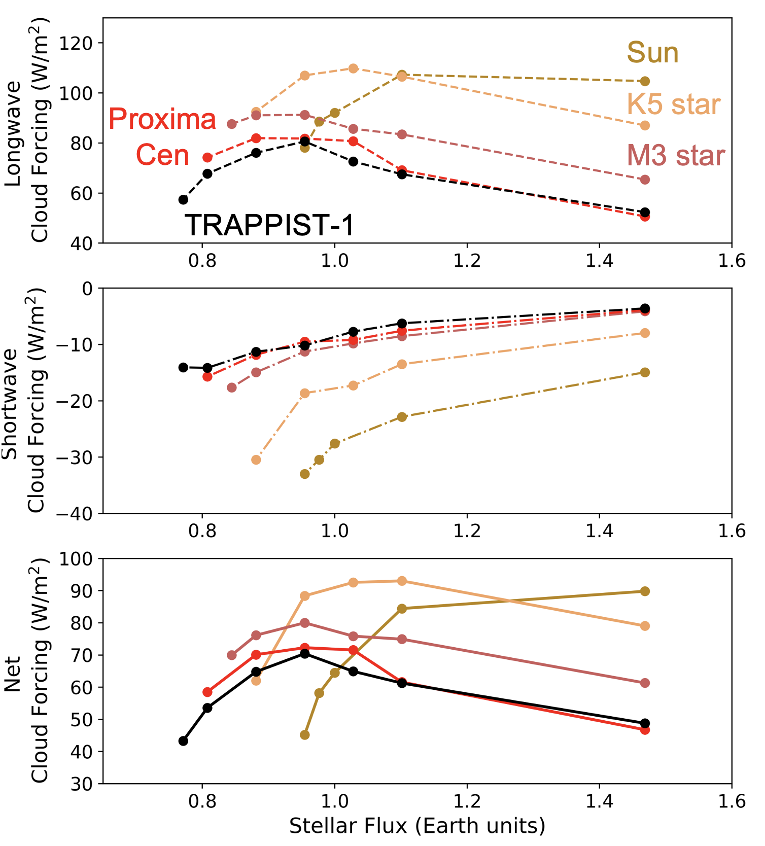
Figure 10: Cloud forcings for initially hot and steamy 1 R_⊕ planets (with a 10 bar of H₂O + 1 bar of N₂ atmosphere) orbiting around different types of stars: TRAPPIST-1 (T_⋆ $\sim$ 2600 K), Proxima Centauri (T_⋆ $\sim$ 3050 K), a M3 star (T_⋆ $\sim$ 3400 K), a K5 star (T_⋆ $\sim$ 4400 K) and the Sun (T_⋆ $\sim$ 5780 K). The associated simulations names are T1-1 to 8, Pcen-1 to 7, M3-1 to 7, K5-1 to 6 and SUN-1 to 6, respectively. The figure depicts the greenhouse effect (top) of clouds, the amount of incident radiation (middle) reflected back by the clouds (the more negative the value, the greater the reflected flux), and the net radiative effect (bottom) of clouds (positive values mean warming), as a function of the incoming stellar flux. In all these simulations, clouds produce a strong atmospheric warming.

It is important to note that the ISR that matters to determine if a planet can condense its primordial water vapour reservoir into oceans is the ISR the planet received at the beginning of the Main Sequence Phase of its host star. This is commonly referred to as the Zero Age Main Sequence (ZAMS). For the types of stars we have studied here, the ZAMS corresponds to the moment when (1) the stellar luminosity is minimal while (2) planets are already fully formed. In Fig. 8, we indicated the ISR of all the currently known planets and exoplanets (with a mass $\leq$ 5 M_⊕ and/or a radius $\leq$ 1.6 R_⊕) in or near the inner boundary of the HZ are shown (black squares), along with the ISR they received at the ZAMS (grey brackets). The planets are based on the following publications: HD85512b (Pepe et al., 2011), GJ667Cc (Bonfils et al., 2013; Anglada-Escudé et al., 2013), $\tau$ Ceti e (Tuomi et al., 2013), Kepler-138e (Rowe et al., 2014; Piaulet et al., 2023), Kepler-442b and Kepler-438b (Torres et al., 2015), K2-3d (Crossfield et al., 2015), Kepler-445d (Muirhead et al., 2015), Proxima b (Anglada-Escudé et al., 2016), K2-72c and e (Dressing et al., 2017), TRAPPIST-1c, d and e (Gillon et al., 2017), Kepler-1652b (Torres et al., 2017), Wolf 1061c, Luyten b (Astudillo-Defru et al., 2017), Kepler-1649b and c (Angelo et al., 2017; Vanderburg et al., 2020), Ross 128b (Bonfils et al., 2018b), GJ 1132c (Bonfils et al., 2018a), Teegarden b (Zechmeister et al., 2019), L98-59e (Kostov et al., 2019), TOI-700d and e Gilbert et al. (2020, 2023), TOI-1266c (Demory et al., 2020), GJ 1061c and d (Dreizler et al., 2020), LP-890-9c (Delrez et al., 2022), Ross 508b (Harakawa et al., 2022), GJ 1002b (Suárez Mascareño et al., 2023), Wolf 1069b (Kossakowski et al., 2023), TOI-715b (Dransfield et al., 2023). While the previous limits of the inner edge of the HZ (Kopparapu et al., 2013; Leconte et al., 2013a; Wolf & Toon, 2015; Kopparapu et al., 2017; Way & Del Genio, 2020) should be compared with the ISR that planets receive today, the water condensation limit (Fig. 8, bold red line) should be compared with the ISR that planets received at the ZAMS.

The ISR of planets at the ZAMS were calculated by (1) using stellar properties, including age estimates and associated uncertainties based on up-to-date publications ; and by (2) calculating the variation in the luminosity of the star between the ZAMS and its current measured age. The grey brackets in Fig. 8 correspond to the $\pm$1$\sigma$ age estimates. For planets for which age constraints are either very loose or non-existent (mostly for low-mass stars), we arbitrarily used age estimates between 1 and 10 Gyr, which is the maximum value in the grid of stellar models of Baraffe et al. 2015). While ISR change significantly with age (between now and the ZAMS) for planets around solar-type and K-type stars, they change very little around low-mass (M-type) stars. Sun-like stars for instance have a luminosity that increases by about 40$\%$ during the first 4.5 Gigayears of evolution in their Main Sequence. Ultra-cool stars like TRAPPIST-1 have an extended Pre-Main-Sequence (PMS) phase during which their luminosity can decrease by more than 2 orders of magnitude within the first Gigayear of evolution (Bolmont et al., 2017). However, once they reach their minimum luminosity (at the ZAMS), then their luminosity increases very little on a time scale less than or equal to the age of the universe.

Fig. 8 illustrates well the findings of Turbet et al. (2021) that (1) Venus never received a low enough insolation to condense its oceans, and (2) that the Earth was able to condense its oceans thanks to the fact that the Sun’s luminosity was fainter in the past than it is today (a.k.a. the Faint Young Sun Opportunity). It also shows that the standard water condensation curve (bold red line in Fig. 8) can be compared directly to the ISR received today by planets orbiting around M stars, because their luminosity evolves very little on the main sequence phase. We predict that several planets (K2-3d, TOI-700d, TOI-700e, K2-72e, Luyten b, LP890-9c, etc.) which are located well inside the Habitable Zone calculated using 3D models for tidally-locked planets (Kopparapu et al., 2017), may in fact never have been able to form surface oceans. Interestingly, for TOI-700d this prediction depends on the age of the planet, which controls the minimum ISR it received at the ZAMS. This result highlights the importance of accurately measuring the age of planetary systems (at least, for planets around early-M and more massive stars) to assess their ability to form oceans in the first place.

In parallel, and to facilitate the usability of our results by the community, we have produced in Fig. 9 a series of water condensation curves at different ages. The curves indicate, for a planet of age X (with X = 0.5, 1, 4.5, and 10 Gyr here), that if that planet is to the left of the age X curve, then it has never been able to, or will never be able to, condense its water at the surface. The numerical values of the curves are provided in Table 2, for further uses. These curves were (1) calculated from the standard water condensation curve (black dashed line in Fig. 9 ; which is the same than the bold red line in Fig. 8) and then (2) multiplied by the ratio $\frac{L_{\star,\text{at age = X}}}{L_{\star,\text{at the ZAMS}}}$. This ratio was determined using the grid of stellar models of Baraffe et al. (2015). We note that the most massive stars in Fig. 9 are too short-lived for the 4.5 and 10 Gigayears limits to be defined. We also note that to evaluate the potential habitability of a planet, the curves in Fig. 9 should be used in tandem with the traditional HZ (Kopparapu et al., 2013, 2017). In the case of planets orbiting around highly evolved stars (for example, the Earth in more than 1 billion year), the inner edge of the Habitable Zone may be more restrictive than the Water Condensation Limit. In other words, the planet may have formed its first oceans by condensation, but then lost them several billion years later when a runaway greenhouse was triggered by the increase in the star’s luminosity (Leconte et al., 2013a; Wolf & Toon, 2015).

Star Type	Water Condensation	WCL at 0.5 Gy	at 1 Gy	at 4.5 Gy	at 10 Gy
	Limit (WCL)
(T${}_{\text{eff}}$)	(F⊕)	(F⊕)	(F⊕)	(F⊕)	(F⊕)
2300	0.772		0.772	0.772	0.775
2400	0.774		0.774	0.774	0.778
2500	0.777		0.777	0.778	0.781
2600	0.779		0.779	0.781	0.783
2700	0.782		0.782	0.783	0.786
2800	0.784		0.784	0.784	0.788
2900	0.787	0.787	0.787	0.789	0.791
3000	0.790	0.790	0.790	0.792	0.795
3100	0.793	0.793	0.793	0.795	0.800
3200	0.796	0.796	0.796	0.800	0.808
3300	0.799	0.799	0.800	0.816	0.838
3400	0.803	0.803	0.806	0.845	0.881
3500	0.806	0.806	0.831	0.858	0.880
3600	0.810	0.810	0.830	0.854	0.876
3700	0.814	0.814	0.824	0.849	0.875
3800	0.817	0.817	0.827	0.856	0.890
3900	0.820	0.820	0.831	0.863	0.905
4000	0.824	0.824	0.836	0.872	0.921
4100	0.828	0.828	0.843	0.884	0.942
4200	0.832	0.832	0.850	0.896	0.964
4300	0.838	0.838	0.859	0.910	0.988
4400	0.843	0.843	0.867	0.923	1.011
4500	0.849	0.850	0.875	0.939	1.037
4600	0.856	0.858	0.885	0.957	1.075
4700	0.863	0.866	0.895	0.976	1.114
4800	0.871	0.875	0.905	0.995	1.155
4900	0.879	0.884	0.916	1.016	1.196
5000	0.888	0.894	0.929	1.046	1.240
5100	0.896	0.903	0.941	1.076	1.325
5200	0.904	0.912	0.953	1.105	1.412
5300	0.911	0.922	0.971	1.134	1.499
5400	0.919	0.932	0.992	1.186	1.588
5500	0.927	0.943	1.014	1.241
5600	0.935	0.962	1.036	1.297
5700	0.943	0.988	1.066	1.354
5800	0.951	1.014	1.096	1.455
5900	0.959	1.040	1.126	1.565
6000	0.968	1.071	1.164	1.709
6100	0.976	1.101	1.203
6200	0.984	1.130	1.242
6300	0.992	1.156	1.281
6400	1.000
6500	1.008

Table 2: Numerical values of the water condensation curves at different ages shown on Fig. 9. We note that the values have been interpolated between the different GCM simulations using the same empirical fit as in Kopparapu et al. (2013) (see main text for more detailed explanations).

In summary, using a grid of GCM simulations, we have defined for the first time a Water Condensation Zone (WCZ), that we propose to use as a new standard to define the inner edge of the HZ. It is fortunate that this limit lies very close – albeit at lower ISR – to the 1D cloud-free calculations of Kopparapu et al. (2013), which are the most widely used definition in the exoplanet community. This is mainly because (1) water vapor profiles are similar between 1D and 3D climate models, and (2) the absence of dayside clouds makes the atmosphere behave as if it were cloud-free from the point of view of shortwave heating. There is also a significant impact (1) of the greenhouse effect of nightside clouds, and (2) of the temporal evolution of stellar luminosity, which both quantitatively affect the water condensation limit (e.g., compared to Kopparapu et al. 2013).

An important point to note is that the question of the ability of planets to condense their primordial atmospheric water vapor reservoir is in fact even more constraining for planets orbiting M-stars (than Sun-like stars), since the level of ISR they receive is much higher during their PMS, which can last up to 1 gigayear (Baraffe et al., 2015) for the lowest mass stars. Indeed, to evaluate the ability of a planet to condense its primordial water reservoir, the water condensation limit should be compared to the minimum ISR received by the planet over the course of its evolution (in general, at the beginning of the Main Sequence Phase, a.k.a. the ZAMS), and not to its currently observed ISR. As a consequence, unlike planets orbiting solar stars, planets around M stars cannot benefit from a lower ISR period at the beginning of their evolution (Turbet et al., 2021) favorable for water condensation. This is well illustrated in Fig. 9 by looking at the difference between the water condensation limit at the ZAMS (dashed black lines), and the water condensation limit at several ages (solid colored lines).

3.5 Application to TRAPPIST-1 planets and their observability with JWST

3.5.1 Water condensation and clouds

We have extended our GCM simulations of H₂O-rich atmospheres to known exoplanets, in particular to TRAPPIST-1 planets (see Table 6 for a detailed list). Fig. 11 shows the cloud distribution, bond albedo and OTR for TRAPPIST-1 inner planets (based on the stellar and planet properties provided in Agol et al. 2021, following Mann et al. 2019 and Ducrot et al. 2020). Again, clouds are located mostly in the nightside, high in the atmosphere. It is clearly visible that the cloud horizontal extension reduces with increasing ISR. The extension of clouds has impacts on the observables – in particular transit spectra – which we discuss in the following subsections.

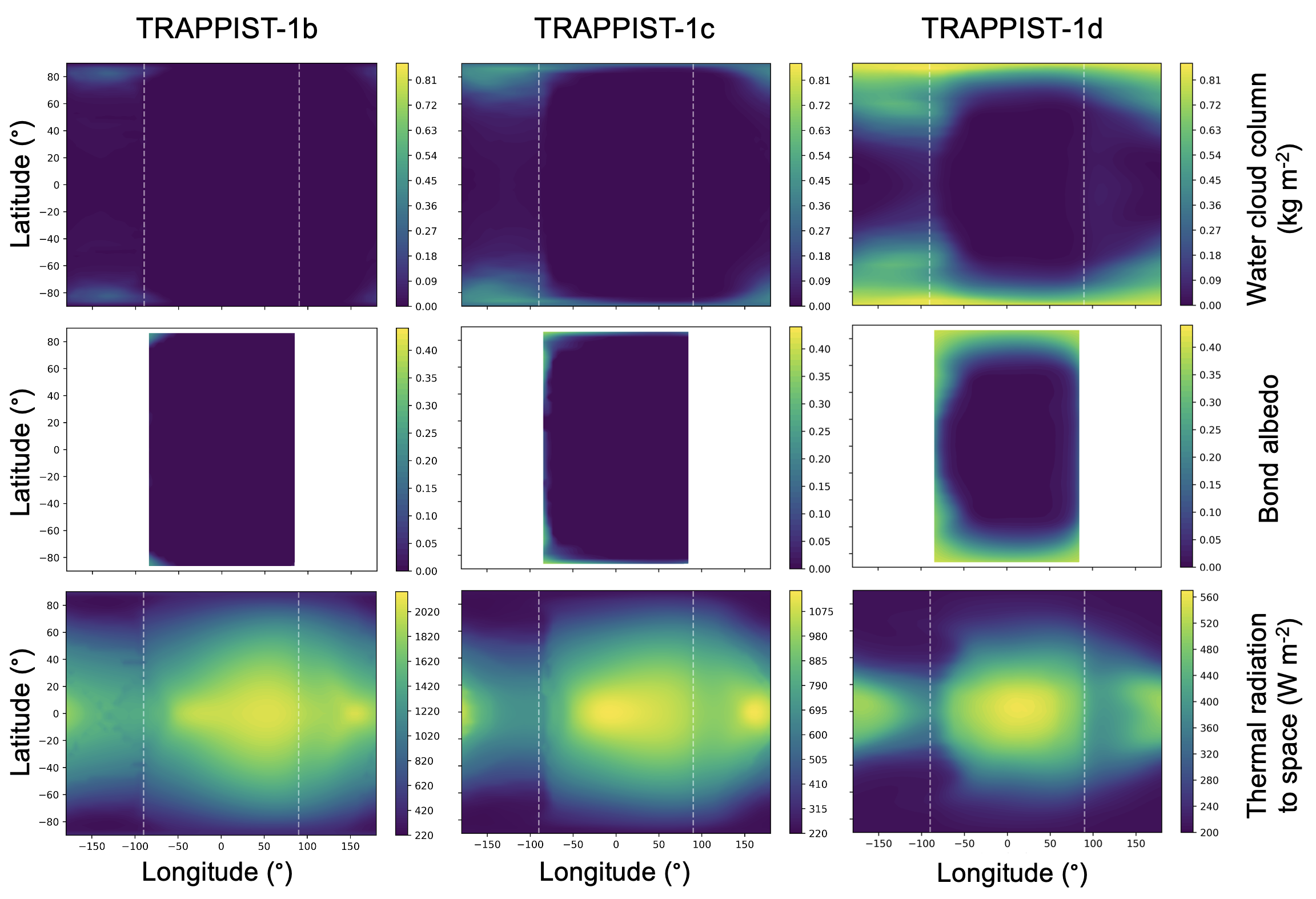
Figure 11: Water cloud column (top), albedo (middle) and thermal emission to space (bottom) horizontal maps, for TRAPPIST-1b (left), TRAPPIST-1c (middle) and TRAPPIST-1d (right). The associated simulations names are T1b, T1c and T1d, respectively. The simulations assume initially hot and steamy tidally-locked planets (with a 10 bar of H₂O + 1 bar of N₂ atmosphere), and the outputs were averaged over 100 Earth days. The dashed white lines indicate the location of the terminator.

For the three TRAPPIST-1 inner planets, in none of the cases that we have explored the water vapor is able to condense on the surface, and thus to form oceans. TRAPPIST-1d, which lies very close to the runaway greenhouse limit (and could be either in or out, depending on subtle cloud feedbacks ; see Wolf 2017; Turbet et al. 2018), is unable to reach the runaway water condensation and should thus lie outside the HZ. Simulations of TRAPPIST-1e (and also Proxima b, for which we also performed a simulation, as it is a prime target for the JWST and the ELTs) systematically lead to the quasi-complete condensation of the water vapor reservoir onto the surface. This confirms what had been calculated in Section 3.2, in the case of an Earth-like planet around TRAPPIST-1, that the water condensation limit is located somewhere between the orbit of TRAPPIST-1d and e. Given that TRAPPIST-1b, c and d are outside of the Water Condensation Zone of their star, they are unlikely to be habitable planets. More generally, there is a significant number of small exoplanets, which had been previously put inside or close to the HZ calculated with 3D models (Kopparapu et al., 2017), and that may never have condensed their primordial water reservoir. This includes TOI-700d (Gilbert et al., 2020), TOI-700e (Gilbert et al., 2023), LP-890-9c (Delrez et al., 2022), Teegarden b (Zechmeister et al., 2019), K2-72e (Dressing et al., 2017), K2-3d (Crossfield et al., 2015), etc.

We have performed several sensitivity simulations to explore the thermal structure of the TRAPPIST-1 planetary atmospheres, summarized in Figs. 12 and 13. Again, our results confirm the 1D accelerated time-marching model results of Selsis et al. (2023) (see a comparison in Extended Data Fig. 3 of Selsis et al. 2023) that the thermal profiles strongly diverge from that calculated from 1D inverse radiative-convective models. In particular, due to the lack of shortwave flux reaching the lower atmosphere and surface, the low atmosphere is much colder than predicted from the adiabatic profile. The water vapor content also has a limited impact on the thermal structure (see Fig.13c). The internal heat flux, which is possibly high on TRAPPIST-1b due to tidal heating (Turbet et al., 2018), has a strong impact on the lower part of the atmosphere (see Fig.13b), by transporting energy from the surface to the upper part of the atmosphere. This brings an extra heating term warming the atmospheric layers near the surface. This confirms with a 3D GCM the results of Selsis et al. (2023). Both the water content and internal heat fluxes (in the range of simulations explored here) have almost no impact on the temperature structure above 0.1 bar as well as on the location and amount of water clouds.

The fact that the thermal profiles calculated with the GCM are very different from the 1D inverse climate calculations has several important consequences (Selsis et al., 2023): reduction of the lifetime of a magma ocean ; modification of the mass-radius relationships, etc.

All the vertical profiles discussed in this Section are used as input of radiative transfer calculations to compute various types of observables (transit spectra, eclipses, phases curves) described in following subsections.

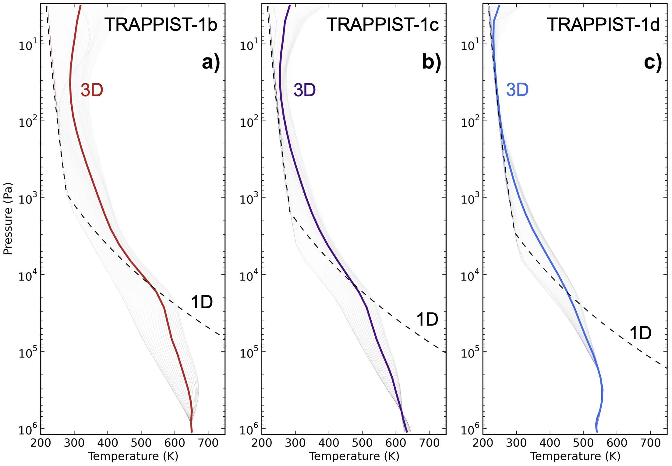
Figure 12: Temperature vertical profiles for TRAPPIST-1b (a), TRAPPIST-1c (b) and TRAPPIST-1d (d). The associated simulations names are T1b, T1c and T1d, respectively. The solid lines are global mean, temporal average (over 100 Earth days) temperature profiles calculated from GCM simulations. The shaded lines are snapshots taken at different latitude and longitude points to show the range of profiles within a simulation. The dashed lines are calculated with a 1D inverse radiative-convective model (Turbet et al., 2019, 2020b), similar to those used in Kopparapu et al. (2013) to calculate the inner edge of the HZ.

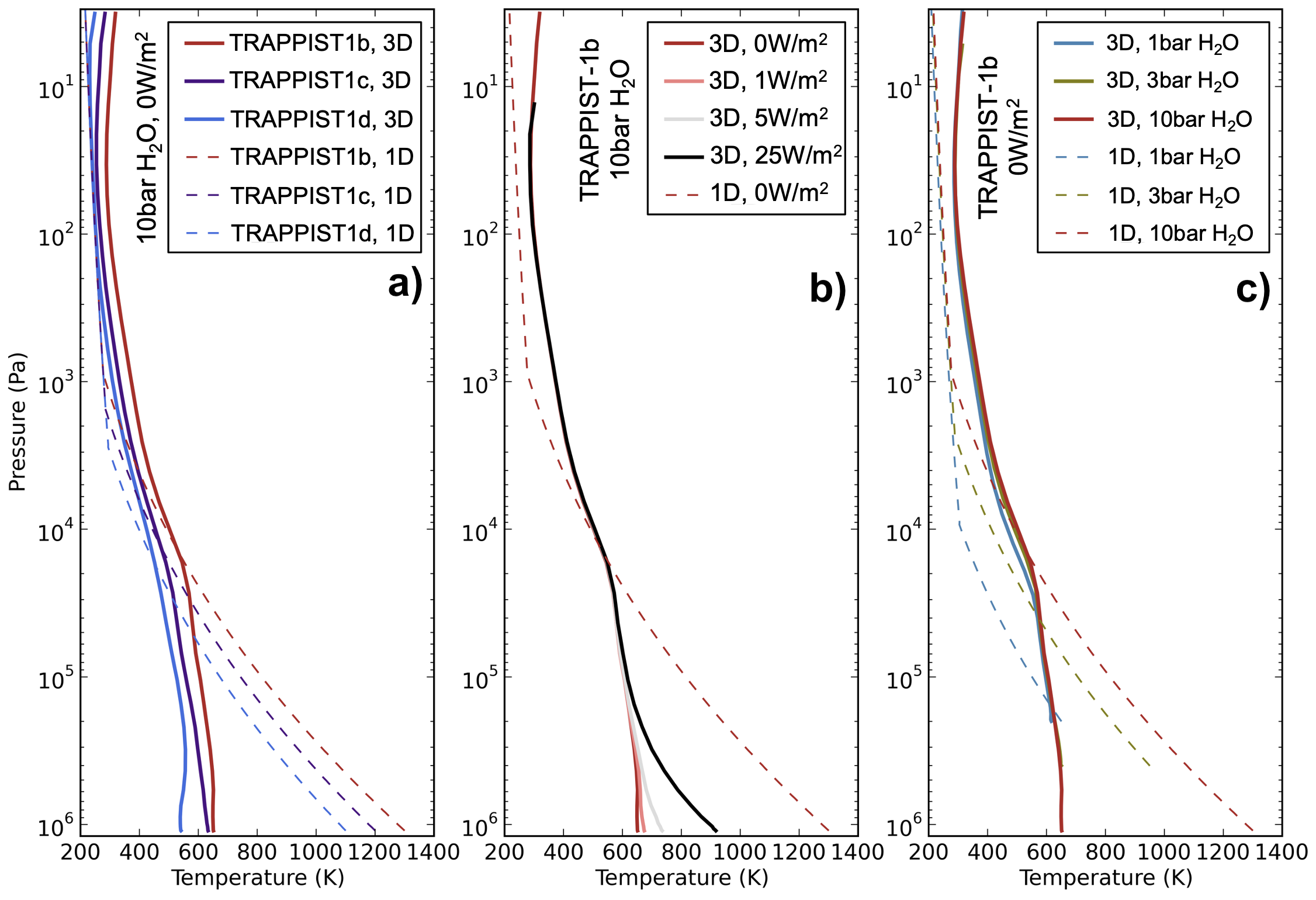
Figure 13: Temperature vertical profiles (a) comparing TRAPPIST-1b, c and d (simulations T1b, T1c and T1d), (b) several internal heat fluxes for TRAPPIST-1b (simulations T1b, T1b-Fgeo1, T1b-Fgeo5 and T1b-Fgeo25), (c) several water partial pressures for TRAPPIST-1b (simulations T1b, T1b-3bar, T1b-1bar). The solid lines are global mean, temporal average (over 100 Earth days) temperature profiles calculated from GCM simulations. The dashed lines are calculated with a 1D inverse radiative-convective model (Turbet et al., 2019, 2020b), similar to those used in Kopparapu et al. (2013) to calculate the inner edge of the HZ.

3.5.2 Transit Spectra

We used the various GCM simulations of TRAPPIST-1b, c and d to compute their expected signature in transit spectroscopy. Fig. 14 summarizes our results for H₂O-dominated atmospheres that we compare – for the context – to spectra for CO₂-dominated atmospheres, calculated also from dedicated GCM simulations (not shown).

Firstly, we observe that the amplitude of water bands in the transit spectra is quite strong, up to 150 ppm for TRAPPIST-1b. We compared our spectra with those of Koll et al. (2019) (calculated between 1.75-3 $\mu$m) for cloud-free H₂O-dominated atmospheres. Our cloud-free spectra (see Fig. 14b, dashed lines) look qualitatively similar. When correcting the amplitude of the transit depth features by the scale height ratio (about 35$\%$ change) using the latest mass measurement of Agol et al. (2021) (compared to that of Grimm et al. 2018), the cloud-free spectra of Koll et al. (2019) are also quantitatively similar to ours. The amplitude of water bands is significantly stronger than that of CO₂ bands (up to 75 ppm for TRAPPIST-1b), due mainly to a larger scale height (with a lower mean molecular weight, and a higher temperature for H₂O than CO₂). We note that the 10 bar CO₂ spectra look qualitatively similar to those of Lustig-Yaeger et al. (2019) and Koll et al. (2019) (calculated between 1.75-3 $\mu$m), although the amplitudes of CO₂ absorption bands are lower. This is again most likely because we used planet properties of Agol et al. (2021), while Lustig-Yaeger et al. (2019) and Koll et al. (2019) used old values (with a higher mass for TRAPPIST-1b) from Grimm et al. (2018). Fig. 14a illustrates that the relative transit depths (i.e. the transit depth corrected from an arbitrary offset) are very similar for the range of atmospheric pressures simulated (from 1 to 10 bar for H₂O, which confirms the results of Koll et al. 2019; from 0.1 to 10 bar for CO₂, which confirms the results of Morley et al. 2017). This is simply due to the fact that the atmospheric structure in the upper atmosphere (i.e. typically for pressures lower than 0.1 bar, which is also the radiative part of the atmosphere, to which transit spectroscopy is most sensitive to) is weakly impacted by the total pressure (see e.g. Fig. 13c). This result differs for CO₂ atmospheres from the predictions of Koll et al. (2019), which used a parameterization of the heat redistribution that produces day-to-night temperature variations significantly larger than what our GCM simulations predict. This impacts the temperature at the terminator, the atmospheric height scale, and thus the amplitude of the molecular bands in the transit spectra as a function of surface pressure.

Secondly, we observe that the impact of clouds varies strongly from one planet to another. This is illustrated in Fig. 14b comparing the transit spectra of TRAPPIST-1b, c, d with and without the effect of clouds (solid versus dashed lines). In fact, the horizontal extension of the clouds (towards the dayside, and thus the terminator regions) increases when decreasing the ISR (see Fig. 11, top row). This is simply because the planet is warmer which reduces the area of cloud stability. The contrast is particularly striking between TRAPPIST-1d – with a significant amount of water clouds reaching the terminator – and the two inner planets, with a lack of clouds. For the TRAPPIST-1 system, we thus find that the ISR required for the water clouds not to significantly blur the transit spectra is somewhere between that of TRAPPIST-1c and d. More generally, we find – using the grid of simulations performed for this study – that removing most water clouds of the terminator requires an ISR typically at least twice that of the Earth.

TRAPPIST-1b, c, d are transit spectroscopy targets of the JWST space-based observatory, starting from Cycle 1, with both NIRSpec and NIRISS instruments. To prepare and anticipate the outcome of these observations, we computed error bars on the synthetic spectra by cumulating all transit observations of JWST Cycle 1, for the three TRAPPIST-1 inner planets (see Figs. 18 and 19). This includes a total of 2 transits of TRAPPIST-1b with NIRISS (Lim et al., 2021), 4 transits of TRAPPIST-1c with NIRSpec (Rathcke et al., 2021) and 2 with NIRISS (Lim et al., 2021), and 2 transits of TRAPPIST-1d with NIRSpec (Lafreniere, 2017). Our spectra reveal that water vapor dominated (i.e., without H₂/He as the dominant gases) atmospheres are theoretically within reach of JWST Cycle 1 observations using transit spectroscopy, for TRAPPIST-1b and c only. For TRAPPIST-1d, the H₂O bands are much weaker due to the effect of clouds forming at the terminator, and a detection would require a larger amount of transits. Detection thresholds are provided in Table 3, for each of the atmospheric scenarios (H₂O and CO₂-dominated atmospheres) and observations planned for the first cycle of JWST. We note that here we did not account for the transit stellar contamination effect (Rackham et al., 2018, 2023), which will be an issue (see review in Turbet et al. 2020a and references therein).

Case	SNR Cycle 1 transits	Number of transits at 5$\leavevmode\nobreak\ \sigma$	Instrument
T1b 0.1 bar CO2	2.9	7	NIRISS
T1b 1 bar CO2	5.1	2	NIRISS
T1b 10 bar CO2	4.7	3	NIRISS
T1b 1 bar H2O	19.2	1	NIRISS
T1b 3 bar H2O	21.3	1	NIRISS
T1b 10 bar H2O	36.8	1	NIRISS
T1c 0.1 bar CO2	1.8	15	NIRISS
T1c 0.1 bar CO2	2.8	13	NIRSpec
T1c 1 bar CO2	3.3	5	NIRISS
T1c 1 bar CO2	4.6	5	NIRSpec
T1c 10 bar CO2	2.4	9	NIRISS
T1c 10 bar CO2	3.5	9	NIRSpec
T1c 10 bar H2O	14.9	1	NIRISS
T1c 10 bar H2O	17.4	1	NIRSpec
T1d 0.1 bar CO2	3.4	5	NIRSpec
T1d 1 bar CO2	5.4	2	NIRSpec
T1d 10 bar CO2	4.4	3	NIRSpec
T1d 10 bar H2O	4.5	3	NIRSpec

Table 3: SNR values to detect an atmosphere assuming Cycle 1 observations and number of transits to achieve a 5$\leavevmode\nobreak\ \sigma$ detection.

Case	SNR Cycle 1 eclipses	SNR Cycle 1 eclipses
	(MIRI F1280W)	(MIRI F1500W)
1b airless 0 albedo	8.7	9.0
1b airless 0.2 albedo	7.6	7.9
1b 0.1 bar CO2	4.3	2.3
1b 1 bar CO2	2.7	2.1
1b 10 bar CO2	2.2	1.9
1b 1 bar H2O	5.6	5.0
1b 3 bar H2O	5.5	5.0
1b 10 bar H2O	5.5	4.9
1c airless 0.2 albedo		5.5
1c 0.1 bar CO2		1.3
1c 1 bar CO2		0.9
1c 10 bar CO2		1.1
1c 10 bar H2O		3.2

Table 4: SNR values to detect a secondary eclipse assuming Cycle 1 observations. Here we corrected the SNR to adjust the Kurucz stellar flux of TRAPPIST-1 in the F1500W MIRI filter to the observed value (Greene et al., 2023; Zieba et al., 2023).

Figure 14: Various transit spectra computed with PSG for the three innermost planets of the TRAPPIST-1 system calculated from 3D GCM simulations (assuming H₂O-dominated composition ; and also CO₂-dominated, for comparison). In the upper panel (a), we compare transit spectra of TRAPPIST-1b for various compositions and pressures ; in the lower panel (b), we compare transit spectra of TRAPPIST-1b, c and d for two compositions only (10 bar H₂O + 1 bar N₂ ; 10 bar CO₂). Dashed lines indicate H₂O cloud-free atmospheres, while solid lines assume H₂O cloudy ones. Dotted lines indicate CO₂ atmospheres (including the effect of CO₂ ice clouds, which is however extremely limited here ; note also that CO₂ condensation was cut off for TRAPPIST-1b and c simulations with 100 mbar of CO₂ as this would cause the atmosphere to collapse on the nightside.). We note that these are relative transit depths (we shifted the curves with arbitrary offsets to compare them more easily).

3.5.3 Secondary Eclipses

Using the same GCM simulations, we computed the expected signals in thermal emission of TRAPPIST-1b and c at the secondary eclipse. Fig. 15 summarizes our results by showing the emission spectra of H₂O-dominated atmospheres compared – for the context – with CO₂-dominated atmospheres, as well as airless planets. TRAPPIST-1b and c are secondary eclipse targets of the JWST, starting from Cycle 1, with the MIRI instrument. This includes a total of 10 eclipses for TRAPPIST-1b (5 in the F1280W filter in Lagage & Bouwman 2017, 5 in the F1500W filter in Greene et al. 2017) and 4 eclipses for TRAPPIST-1c in the F1500W filter (Kreidberg et al., 2021). We have added in Fig. 15 the first results of this observational campaign in the F1500W filter for TRAPPIST-1b (Greene et al., 2023) and TRAPPIST-1c (Zieba et al., 2023). We note that in Fig. 15 we have artificially reduced the observed secondary eclipses of TRAPPIST-1b and c by 9.8$\%$ to correct for the difference between the observed stellar flux in the MIRI F1500W filter (equal to 2.595 mJy, based on Greene et al. 2023 and Zieba et al. 2023 which provide an absolute stellar flux in very good agreement) and that predicted by the stellar spectra used for TRAPPIST-1 (using Kurucz 2005 stellar templates). We computed error bars near 15 $\mu$m (F1500W MIRI filter) on the synthetic spectra by using the observed values from Greene et al. (2023) for TRAPPIST-1b ($\pm$ 99 ppm) and from Zieba et al. (2023) for TRAPPIST-1c ($\pm$ 94 ppm), divided by the square root of the ratio between the synthetic Kurucz stellar spectrum of TRAPPIST-1 and the observed stellar flux in the MIRI F1500W filter (Greene et al., 2023; Zieba et al., 2023). For TRAPPIST-1b, we evaluated the error bars near 12.8 $\mu$m (F1280W MIRI filter) by using the error bars near 15 $\mu$m (F1500W MIRI filter) rescaled by the square root of the ratio of synthetic Kurucz stellar fluxes between F1280W and F1500W filters.

We observe that the eclipse depth is strong for H₂O-rich atmospheres (up to 400 ppm and 250 ppm for TRAPPIST-1b and c, respectively, near 15 $\mu$m). We note that the spectra are very similar for the explored atmospheric pressure range (from 1 to 10 bar of H₂O, which confirms the results of Koll et al. 2019 for TRAPPIST-1b, calculated between 5-12 $\mu$m). This is because most of the planetary thermal emission comes from atmospheric layers at or above 1 bar (Boukrouche et al., 2021). In fact, we are not sensitive here to the contribution of the surface thermal emission (Hamano et al., 2015) because the surface is not hot enough to emit in the visible. This result is likely to persist even for water contents well above 10 bar (Selsis et al., 2023).

By comparison, emission spectra of CO₂-dominated atmospheres exhibit stronger variations when changing surface pressure, which confirms the results of Koll et al. (2019) (calculated between 5-12 $\mu$m) and Ih et al. (2023) (for TRAPPIST-1b). This is due to the fact that CO₂-dominated atmospheres have many more spectral windows (compared to H₂O), where the planetary thermal emission is thus sensitive to the surface temperatures (which depends on the greenhouse effect of CO₂, and thus on the total pressure of CO₂). It is clearly visible in Fig. 15 that CO₂ spectra look similar in the CO₂ absorption bands (e.g., near 15 $\mu$m), but look different in the CO₂ spectral windows.

Our emission spectra reveal that for the two planets, CO₂, H₂O and airless atmospheres leave distinct signatures, which are detectable by the MIRI instrument onboard JWST (see Table 4). The differences between our simulated cases are particularly strong near 15$\mu$m, where JWST Cycle 1 observations have been obtained for the two planets (Greene et al., 2023; Zieba et al., 2023). Our GCM-based calculations confirm that thick CO₂-dominated atmospheres are unlikely for TRAPPIST-1b and c (rejected at $>$ 6 $\sigma$ for TRAPPIST-1b ; rejected at $>$ 3 $\sigma$ for TRAPPIST-1c). While a thick H₂O-dominated atmosphere is also unlikely for TRAPPIST-1b (rejected at $>$ 3 $\sigma$), it is compatible within $\sim$1 $\sigma$ with the F1500W MIRI observations of TRAPPIST-1c. This makes TRAPPIST-1c a promising candidate to test the existence of water vapor and clouds using transit spectroscopy as well as secondary eclipses in other MIRI filters.

To isolate the contribution of the planet (and thus get rid of corrections on the stellar flux), and facilitate comparison with previous works (Lustig-Yaeger et al., 2019), we have converted the eclipse depths into brightness temperatures. This was done by first (1) computing a grid of secondary eclipse spectra at fixed brightness temperatures (to get the correspondence between eclipse depth and brightness temperature), and then (2) interpolating our thermal emission spectra (based on GCM simulations) using this grid. Fig. 16 summarizes our results for TRAPPIST-1b and c, along with published observations (Greene et al., 2023; Zieba et al., 2023). We note that we have recalculated the observed brightness temperatures and found values a few degrees lower than in Greene et al. (2023) and Zieba et al. (2023) ($493^{+26}_{-26}$ K instead of $503^{+26}_{-27}$ K for TRAPPIST-1b ; $376^{+31}_{-33}$ K instead of $380^{+31}_{-31}$ K for TRAPPIST-1c). In our brightness temperature calculations, we aimed at treating observations and models using the same procedure in order to make comparisons as fair as possible. We thus computed first, for a grid of brightness temperatures, a grid of eclipse depth spectra. We then converted the grid of spectra into a grid of F1500W MIRI eclipse depths by integrating the fluxes in the F1500W MIRI filter. Finally, we interpolated in this grid using the measured F1500W eclipse depth values (of Greene et al. 2023 for the TRAPPIST-1b grid ; of Zieba et al. (2023) for the TRAPPIST-1c grid) to derive the observed brightness temperatures. For CO₂-dominated atmospheres (at least the 10 bar simulation), we find results that are qualitatively similar to Lustig-Yaeger et al. (2019). Most differences are likely due to different atmospheric compositions used (e.g., Lustig-Yaeger et al. 2019 have lower brightness temperature near 8.5 $\mu$m likely due to SO₂ absorption included), which makes it difficult to compare other effects (3D vs 1D for example). We note that although the measurements at 15 $\mu$m are incompatible for TRAPPIST-1b with almost all our models of CO₂ and H₂O atmospheres, this does not demonstrate the absence of an atmosphere that could have a composition very different from that explored in the present manuscript.

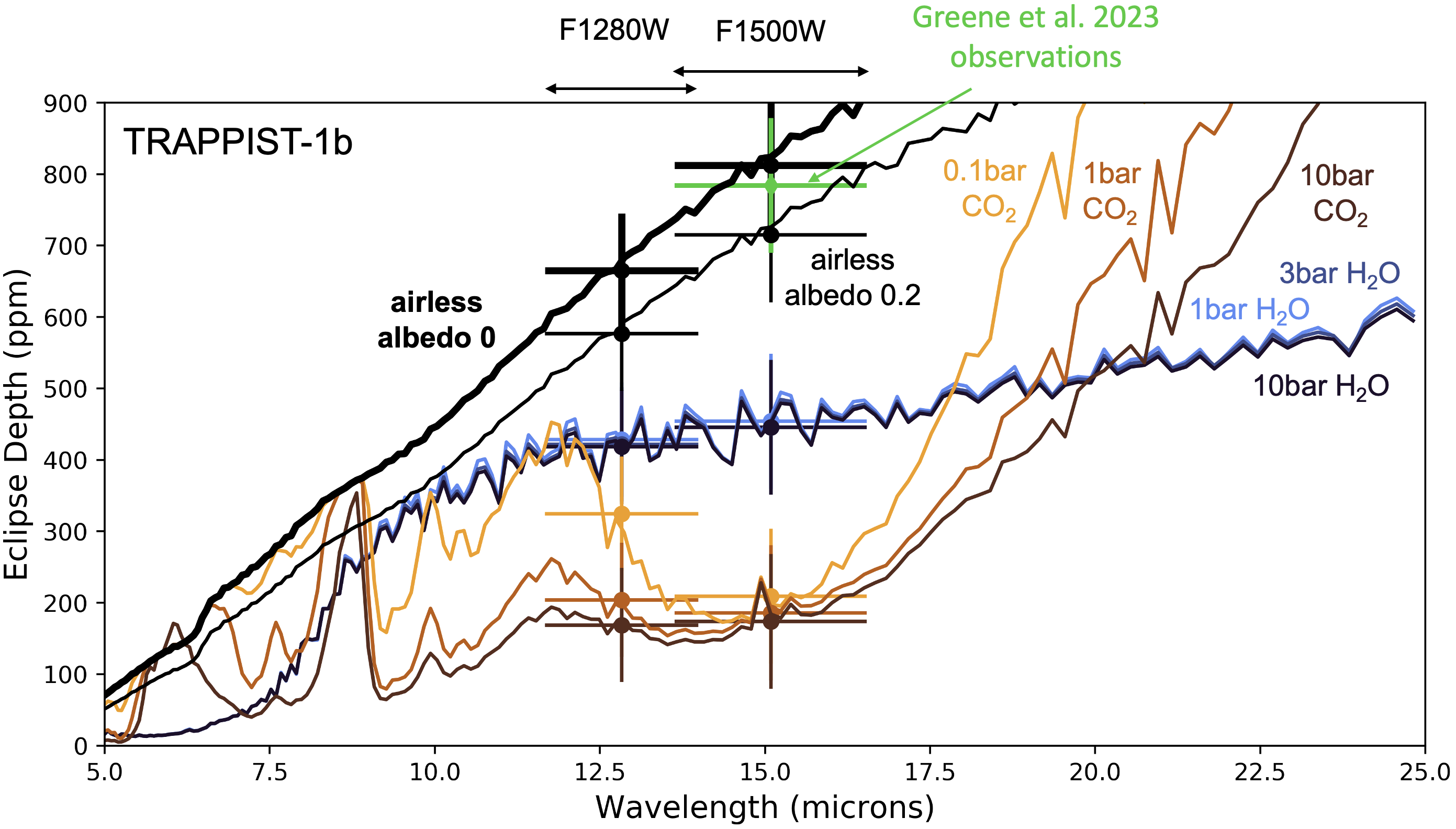
(a)

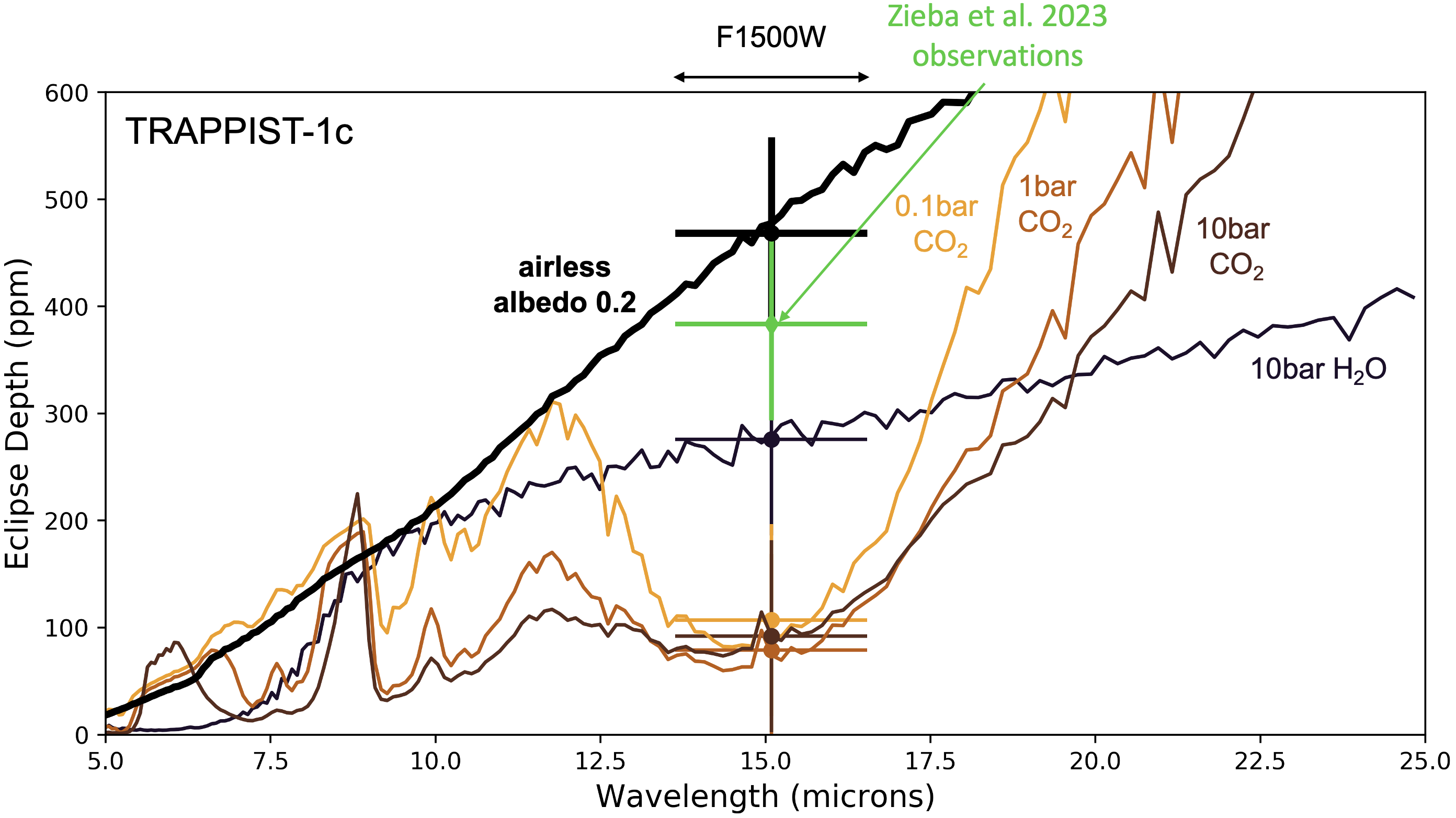
(b)

Figure 15: Emission spectra of TRAPPIST-1b (upper panel) and c (lower panel), calculated at the secondary eclipse. The spectra are calculated using GCM simulations of H₂O-rich (blue to grey colors) and CO₂-rich atmospheres (red to orange colors). Emission spectra are also computed for airless planets (in bold black). 1-$\sigma$ error bars are calculated using the JWST Cycle 1 observation program (more details in Section-3.5.3).

(a)

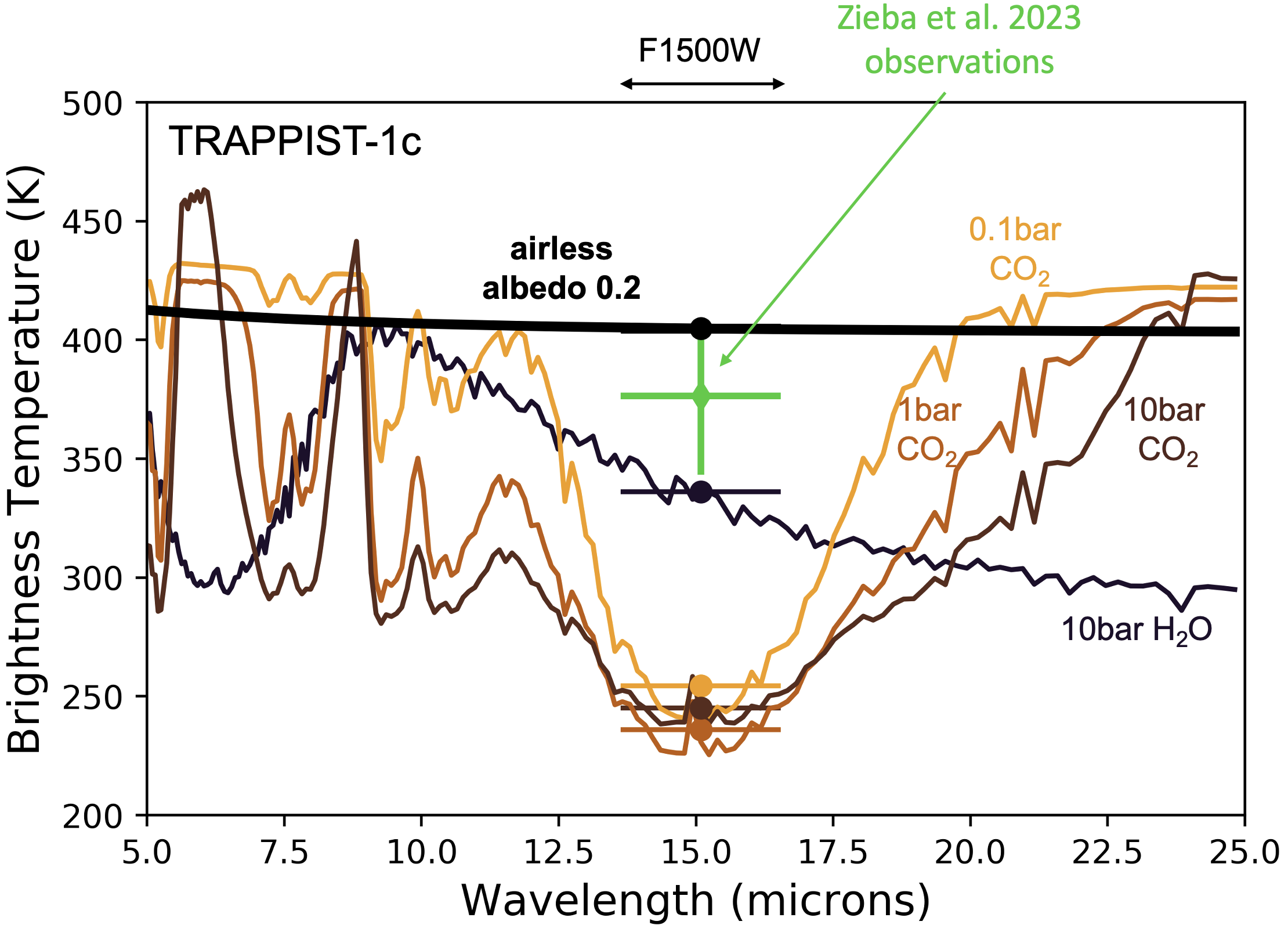
(b)

Figure 16: Same as Fig. 15, with the emission converted in brightness temperature units.

3.5.4 Phase Curves

Last but not least, using again the same GCM simulations, we computed their expected signals in thermal phase curves. Such observations are planned for the Cycle 2 of JWST (Program 3077, 55 hours of observations ; i.e. about 1 orbit of TRAPPIST-1c or 1.5 orbit of TRAPPIST-1b) with the MIRI instrument using the F1500W filter. This observation mode is a promising avenue to characterize the atmospheres of TRAPPIST-1b and c. Fig. 17 summarizes our results by showing the thermal emission phase curves of H₂O-dominated atmospheres compared – for the context – with CO₂-dominated atmospheres, as well as airless planets. For this figure, we have integrated the thermal emission on the F1500W filter (centered around 15 $\mu$m) as it is the selected observing mode for the phase curve measurements to be obtained within JWST Cycle 2.

There are significant differences between the different types of atmospheres. The phase curves of H₂O-dominated atmospheres have relatively low day-to-night amplitudes. For TRAPPIST-1b, c and d, there is a factor of 1.7 to 2 (in the F1500W filter) between dayside and nightside emissions. We interpret this behaviour, which is similar to what is observed in Wolf et al. (2019) for the incipient runaway case, as follows. At first order, the signal of the phase curve can be decomposed into two parts, (1) a continuous signal (which persists at all phase angles) corresponding to the thermal emission of the Simpson-Nakajima limit (Nakajima et al., 1992; Goldblatt & Watson, 2012) ; (2) a second source of emission localized on the dayside, which is produced by the re-emission of the ISR absorbed high in the atmosphere (Wolf et al., 2019). In fact, the first component is lower than the Simpson-Nakajima limit due to part of the emission being absorbed by nightside clouds. This is well visible by looking at the OTR maps in Fig. 1, 4 and 11 (bottom rows). The presence of nightside water clouds reduces in fact the planet’s thermal emission on the nightside, leaving a visible signature on the phase curve. The effect is qualitatively comparable to that of silicate clouds on the phase curves of hot giant exoplanets (Parmentier et al., 2021). Clouds are more prominent and thus have a stronger impact on the phase curves for planets receiving an insolation close to the water condensation limit.

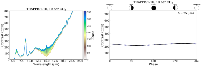
(a)

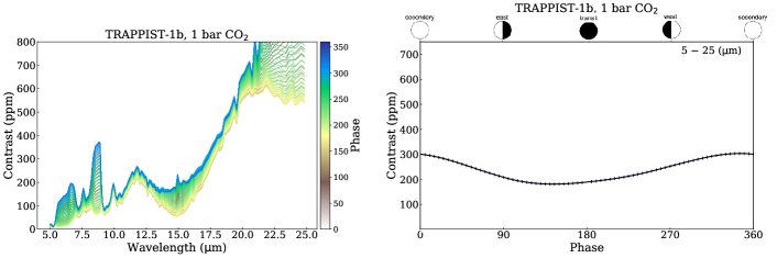
(b)

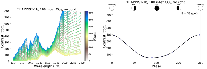
(c)

Figure 21: Thermal emission spectra at various phase angles (left). Thermal phase curve (right) integrated over all wavelengths.

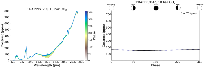
(a)

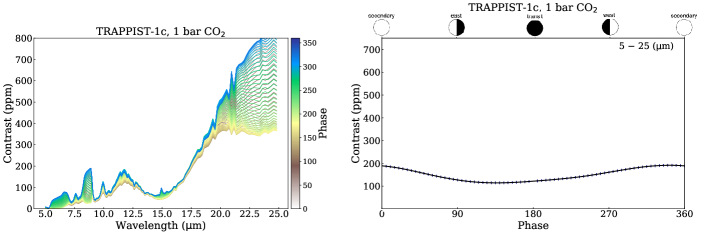
(b)

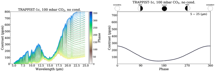
(c)

Figure 24: Thermal emission spectra at various phase angles (left). Thermal phase curve (right) integrated over all wavelengths.

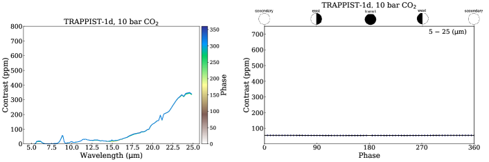
(a)

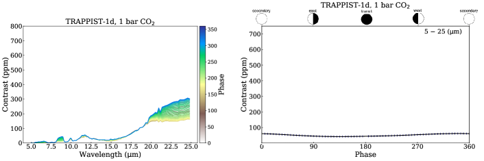
(b)

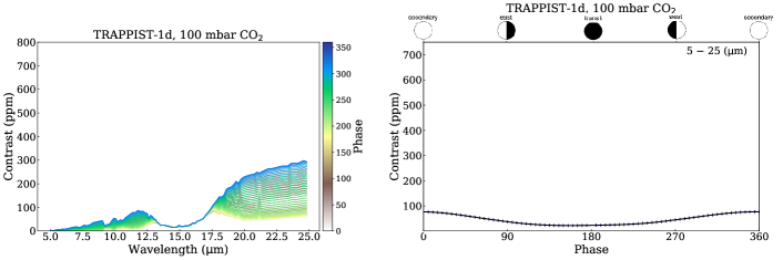
(c)

Figure 26: Thermal emission spectra at various phase angles (left). Thermal phase curve (right) integrated over all wavelengths.

Again, we note that the phase curves look very similar for all the surface pressures explored (from 1 to 10 bar of H₂O). Interestingly, we observe a significant hotspot phase shift in the H₂O-rich simulations (which is less pronounced in the CO₂ phase curves). We interpret this hotspot shift as a consequence of the stellar flux being absorbed high in the atmosphere (combined with the effect of the mean molecular weight ; see Zhang & Showman 2017). This is because (1) the shortwave heating combined with rotation rate produce strong westerly winds transporting heat from the day to the nightside. This is well illustrated in Fig. 2 that shows the strong horizontal winds in the stratosphere. This is also because (2) the thermal emission comes from low pressure atmospheric layers, where horizontal winds are strong. Interestingly, CO₂-dominated cases have a much less pronounced hotspot offset (near 15 $\mu$m, which is the strongest CO₂ absorption band), mostly due to the fact that atmospheric winds are much weaker due to less shortwave flux being absorbed high in the atmosphere (where most of the OTR is emitted at 15 $\mu$m). The amplitude of the phase curve and hotspot offset depend of course on the wavelength considered. This is well illustrated in the Figs. 21, 24, 26.

We note that the simulated emission spectra of TRAPPIST-1b, c and d are provided at different phase angles (including at secondary eclipse, discussed in the previous Section) in Fig. 20 to 26).

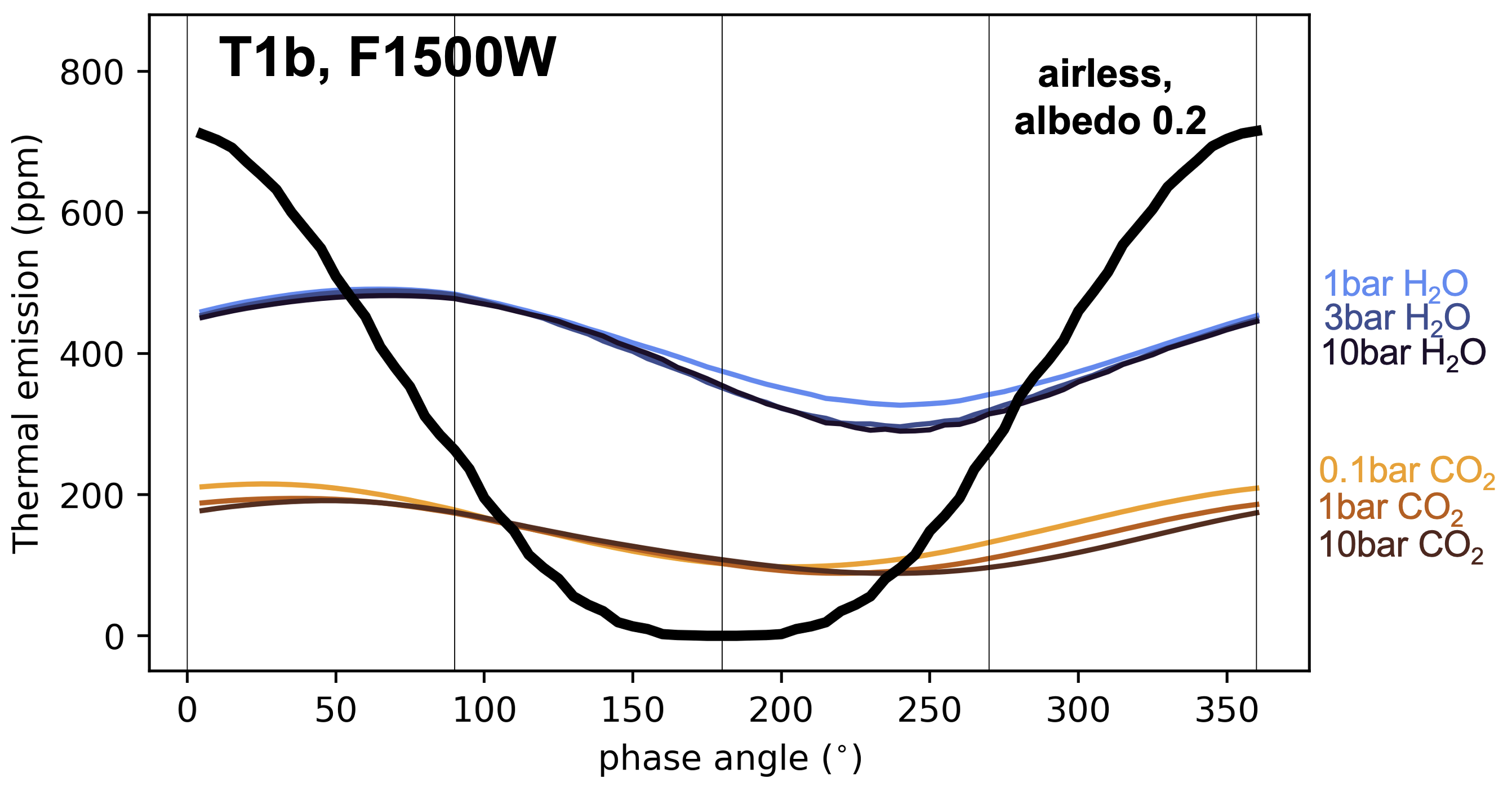
(a)

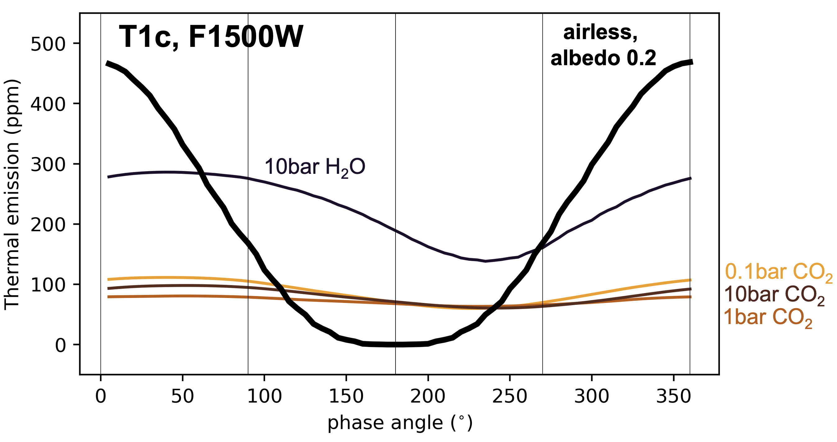
(b)

Figure 17: Thermal phase curves of TRAPPIST-1b (upper panel) and c (lower panel), integrated in the F1500W filter (centered around 15$\mu$m), for various atmospheric scenarios: H₂O-rich (blue to grey colors), CO₂-rich atmospheres (red to orange colors), airless planet (bold black color). H₂O-rich atmospheres also include 1 bar of N₂.

4 Discussions

4.1 Comparisons with other GCMs

3D simulations in Turbet et al. (2021) and in this study were performed with the same GCM: The Generic PCM. This raises the question of whether nighside cloud formation in H₂O-dominated atmospheres is also obtained in other 3D climate models. The multi-model validation (Fauchez et al., 2020, 2021) is indeed a crucial step to validate this cloud effect, which has potentially strong impacts on the habitability of planets (Turbet et al., 2021; Kasting & Harman, 2021). The best illustration of this multi-model approach is the demonstration that substellar convective clouds appear in all models that have simulated a synchronously rotating aquaplanet, giving great confidence in this cloud feedback (see GCM intercomparisons in Yang et al. 2019b; Sergeev et al. 2022).

We thus surveyed the literature to look for evidence (or absence of evidence) of a similar cloud feedback regarding the formation of nightside water clouds in other models. First of all, and to the best of our knowledge and except in Turbet et al. (2021), there are no published results of 3D GCM simulations of post-runaway atmospheres (i.e. water-dominated atmospheres with an exhausted surface water reservoir). Boukrouche (2022) (PhD manuscript) recently performed cloud-free GCM simulations of post-runaway water-dominated atmospheres and confirmed – using the ExoFMS-SOCRATES GCM – the preferential formation of clouds on the nightside, based on distance to saturation. Apart from this work, the best analogues we have can be found in numerical studies that simulated the climate of planets in incipient runaway greenhouse (Kopparapu et al., 2017; Wolf, 2017; Wolf et al., 2019; Kane, 2022; Chaverot et al., 2023). Using the ExoCAM GCM, Kopparapu et al. (2017) first studied the climate and clouds of tidally-locked rocky exoplanets transitioning into the runaway greenhouse. They found that as soon as a planet reaches the runaway greenhouse transition, its substellar convective cloud layer dissipates, drastically reducing the albedo and accelerating the runaway greenhouse. The same effect is also seen with ExoCAM in Wolf (2017) with GCM simulations of TRAPPIST-1d. A snapshot of cloud distribution on TRAPPIST-1d as it evolves into the runaway greenhouse transition (see Wolf 2017, Fig. 4) not only reveal the absence of clouds on the dayside, but also a preferential accumulation of clouds on the nightside, with two local maxima near the wind gyre structures, similar to our findings. Similar cloud distributions are obtained again with ExoCAM (see Wolf et al. 2019, Figs. 4 and 5), for a broader range of host star types (from T${}_{\text{eff}}$ = 2600 K to 4500 K). Using ROCKE-3D GCM, Kane et al. (2018) also performed GCM simulations of the exoplanet Kepler-1649b in incipient runaway greenhouse. The runaway greenhouse produces a sharp decrease of the bond albedo. We analyzed the netCDF simulation file, provided in Kane (2022), and that reveals that water clouds are also preferentially located on the nightside in the upper part of the atmosphere.

In summary, our literature review reveals that the preferential formation of nightside clouds is also obtained in other GCMs (ExoCAM, ROCKE-3D, ExoFMS) as soon as they reach conditions where water vapor becomes a dominant gas in the atmosphere (in the so-called incipient runaway greenhouse). This cloud feedback of course deserves to be studied and validated in the context of post-runaway water-dominated atmospheres with other GCMs (including the effects of water clouds).

4.2 Detecting the cloud feedback

Our simulations of synthetic spectra (see Sections 3.5.2, 3.5.3 and 3.5.4) reveal that JWST has the capability of probing water-rich atmospheres around TRAPPIST-1b, c and d either in transit spectra or in emission. Observations are particularly favorable for TRAPPIST-1b and c, because the ISR received on the planets is high enough (1) to suppress cloud at the terminator and thus strongly increase the amplitude of water bands in transit spectra ; and (2) to increase the temperatures, and thus the thermal emission of the planets. Measurements at 15 $\mu$m (MIRI F1500W filter) show however that a thick H₂O-dominated atmosphere is unlikely for TRAPPIST-1b (rejected at $>$ 3 $\sigma$) leaving TRAPPIST-1c as the best candidate so far (compatible at $\sim$1 $\sigma$). For TRAPPIST-1d, the observations are more difficult not only because the planet is smaller and cooler, but also because water clouds blur the transit spectra. However, by accumulating enough transits (see Table 3), transit spectra could reveal the presence of water vapour. Together, comparative observations of TRAPPIST-1 inner planets (planet c versus planet d) could be used to reveal the presence of nightside clouds, in case their composition turn out to be dominated by water vapor.

Although we used the TRAPPIST-1 planets as targets to compute observables, more easily accessible targets such as water-rich mini-Neptunes (Luque & Pallé, 2022) could be used to detect this cloud effect, in particular by comparing observations of planets at different values of ISR. We identified indeed a threshold ISR, around 2$\times$ the insolation on Earth (the exact value depends on many factors that deserve to be explored in more details), above which water clouds become significantly depleted at the terminator, significantly increasing the amplitude of absorption features in transit spectra. Based on the simulations we did, we also identified another threshold ISR, around 5$\times$ the insolation on Earth, above which water clouds entirely disappear. Although these ISR thresholds may vary from one planet to another, depending on its amount of water vapor, its size, its type of star, etc., we looked for planets in this ISR range with the best observability metrics, using the ESM (Emission Spectroscopy Metrics) and TSM (Transmission Spectroscopy Metrics) of Kempton et al. (2018). In addition to the three inner planets of the TRAPPIST-1 (which are the planets with the best TSM and amonst the best ESM), we have identified LP 791-18c (Crossfield et al., 2019; Peterson et al., 2023), TOI-270d (Günther et al., 2019) and LTT 3780c (Cloutier et al., 2020). These three planets have radii between 2.1 and 2.4$\times$ that of the Earth and their density is compatible with the presence of both water and hydrogen envelopes. If these planets happen to be enriched in water, then they could serve as a natural laboratory for testing the behavior of water clouds, using transit spectra, secondary eclipses and phase curves. Previous simulations of K2-18b with the Generic PCM (Charnay et al., 2021) show indeed qualitatively similar cloud behaviour for temperate mini-Neptune with atmospheric composition of very high metallicity ($>$300). At lower metallicity, clouds can form on the dayside essentially due to two factors (Charnay et al., 2015a, b): (1) less water vapour induces less radiative heating on the dayside and less radiative cooling on the nightside ; (2) the specific heat capacity decreases due to higher mixing ratios of hydrogen and helium, which further reduces the day-to-night temperature contrast.

Detecting the water cloud feedback – using TRAPPIST-1 planets or any population of planets endowed with water-rich atmospheres – would have profound consequences for our understanding of the habitability of exoplanets, but also of that of the solar system planets (Earth vs Venus).

4.3 Caveats

In this study, we explored the ability of exoplanets to form their first oceans by simulating the condensation of the primordial water reservoir at the end of the magma ocean phase (Hamano et al., 2013; Lichtenberg et al., 2023).

In Turbet et al. (2021) and this new study, we have performed several sensitivity studies, including: varying the amount of CCN (Turbet et al., 2021) ; varying the amount of water (this work ; Turbet et al. 2021), of carbon dioxide (Turbet et al., 2021). However, to build confidence in these simulations, more sensitivity studies are needed. Firstly, one can question the choice of parameterizations used in this work. Previous works (Yang et al., 2019b; Sergeev et al., 2020, 2022) have shown, for example, that the choice of moist convection scheme has strong consequences on the properties of the substellar cloud layer predicted in the ‘cold start’ simulations. Cloud formation in our ‘hot start’ Generic PCM simulations is largely dominated by large-scale condensation (that is, water vapour condensation driven by large-scale air movements) and not by subgrid-scale condensation (driven by small convective cells, and parameterized using our moist convection scheme). This indicates that our results should be weakly sensitive to the choice of the subgrid moist convection parameterization, which is a strong indication that preferential nightside cloud formation is likely to be a robust mechanism across GCMs (see Section 4.1). However, this deserves to be tested in detail with other GCMs as well as with cloud-resolving simulations (Tan et al., 2021). Secondly, one can question the choice of atmospheric compositions used in this work. It has been shown that various atmospheric compositions could be expected at the end of the magma ocean phase, depending on the redox state (Bower et al., 2022). Modeling a wider range of atmospheric compositions, more representative of all the possible post-magma scenarios, is therefore a necessary step to validate our results.

Moreover, even if the primordial water reservoir never condensed, it is possible that late volcanic degassing, or volatile delivery by cometary impacts, could bring water contributing to form surface oceans (Moore & Cowan, 2020). This would probably require the planet to have lost its atmosphere at some point – temporarily transforming the planet into a so-called land planet (Kodama et al., 2015) – otherwise the delivered water would probably remain vaporized. This scenario also deserves to be explored in details, at least in part with the help of dedicated 3D numerical climate simulations.

5 Conclusions

In this study, we used the 3D Generic Planetary Climate Model to perform a large grid of simulations for H₂O-dominated atmospheres planets orbiting around a wide variety of Main-Sequence stars. The simulations were designed to reproduce the conditions of early ocean formation on rocky planets due to the condensation of the primordial water reservoir at the end of the magma ocean phase (Hamano et al., 2013; Lichtenberg et al., 2023).

So far, all Global Climate Model (GCM) simulations – assuming the entire water reservoir is initially fully condensed on the surface – have shown that low-altitude dayside convective clouds stabilize oceans even at high incoming stellar radiation (ISR) (Yang et al., 2013, 2014; Kopparapu et al., 2016, 2017; Way et al., 2016; Yang et al., 2019b, a; Sergeev et al., 2020, 2022). In contrast, our new GCM simulations – assuming the entire water reservoir is initially fully vaporized in the atmosphere – show that high-altitude nightside stratospheric clouds prevent surface water condensation from happening even at low ISR. This behaviour was already observed by Turbet et al. (2021) in the case of early Earth and Venus, and we thus extend it here to synchronously-rotating planets around all types of Main-Sequence stars (M, K and G types). More generally, this confirms and extends the results of Turbet et al. (2021) that the formation of nightside clouds seem to occur independently of the rotation rate assumed. Future work could test up to what rotation rate this result holds, given that there should be a threshold rotation rate above which Coriolis forces inhibit day-night stratospheric transport. This is particularly relevant for young planets, which are likely to have a much faster rotation rate than that determined by synchronous rotation. We propose to name this family of planets ”mochi planets”, with the planetary surface represented by red bean paste, and the cloud layer represented by the sticky rice in which someone has taken a bite. Yummy!

Based on these results, we introduced a Water Condensation Zone (WCZ), whose inner edge is located at lower ISR than the inner edge of the Habitable Zone (HZ). In other words, we found that the ISR required to form oceans by condensation is always significantly lower than that required to vaporize oceans. The contrast is particularly striking with all the recent 3D GCM results that assume most water is initially on the planetary surface (Yang et al., 2013, 2014; Kopparapu et al., 2016, 2017; Way et al., 2016). Interestingly, the inner edge of the WCZ lies quite close (but still at lower ISR, due to the greenhouse effect of nightside clouds) to the – widely used – inner edge of the HZ of Kopparapu et al. (2013), based on 1D cloud-free calculations. This is mainly because (1) water vapor profiles are similar between 1D and 3D climate models, and (2) the absence of dayside clouds makes the atmosphere behave as if it were cloud-free from the point of view of shortwave heating.

We confirm with 3D GCM simulations the results of Selsis et al. (2023) that in thick H₂O-dominated atmospheres, the vertical thermal profile diverges from that calculated using 1D inverse radiative-convective models (Kopparapu et al., 2013; Turbet et al., 2019; Boukrouche et al., 2021). This has important consequences for the lifetime of the magma ocean period, as well as the calculations of mass-radius relationships for irradiated planets (Turbet et al., 2020b).

Last but not least, we show – taking the inner planets of the TRAPPIST-1 system as an example – that the JWST has the capability to probe water-rich atmospheres. We identify a threshold insolation, around 2 times the insolation on Earth (the exact value depends on many factors), above which water clouds disappear from the terminator, significantly increasing the amplitude of absorption features in transit spectra. For the TRAPPIST-1 system, we predict the transition occurs between TRAPPIST-1c and d. JWST observations using transit spectroscopy, but also secondary eclipses and thermal phase curves, can be used to probe first the existence of water-rich atmospheres on TRAPPIST-1 inner planets, and eventually test the existence of the nightside cloud feedback. Although we used the TRAPPIST-1 planets as a testbed, other accessible targets such as water-rich mini-Neptunes (Luque & Pallé, 2022) could be used to detect this cloud effect. This would have profound consequences for our understanding of the habitability of exoplanets, but also of that of the solar system planets (Earth vs Venus).

Appendix A Additional Tables

We provide here – in Tables 5 and 6 – the main list of 3D Global Climate Model (GCM) simulations performed with the Generic PCM in this study.

Simulation	Star Type (T${}_{\text{eff}}$)	Flux	Rotation Period	Mass	Radius	P${}_{\rm H_{2}O}$	Internal heat flux
Name	(K)	(F⊕)	(Earth days)	(M⊕)	(R⊕)	(bar)	(W m-2)
SUN-1	Sun (5780)	1.47	1 (non-TL)	1	1	10	0
SUN-2	Sun (5780)	1.10	1 (non-TL)	1	1	10	0
SUN-3	Sun (5780)	1.00	1 (non-TL)	1	1	10	0
SUN-4	Sun (5780)	0.98	1 (non-TL)	1	1	10	0
SUN-5	Sun (5780)	0.95	1 (non-TL)	1	1	10	0
SUN-6	Sun (5780)	0.92	1 (non-TL)	1	1	10	0
K5-1	K5 (4400)	1.47	87.0 (TL)	1	1	10	0
K5-2	K5 (4400)	1.10	108.0 (TL)	1	1	10	0
K5-3	K5 (4400)	1.03	113.7 (TL)	1	1	10	0
K5-4	K5 (4400)	0.95	120.2 (TL)	1	1	10	0
K5-5	K5 (4400)	0.88	127.6 (TL)	1	1	10	0
K5-6	K5 (4400)	0.84	131.8 (TL)	1	1	10	0
M3-1	M3 (3400)	1.47	18.3 (TL)	1	1	10	0
M3-2	M3 (3400)	1.10	22.7 (TL)	1	1	10	0
M3-3	M3 (3400)	1.03	23.9 (TL)	1	1	10	0
M3-4	M3 (3400)	0.95	25.2 (TL)	1	1	10	0
M3-5	M3 (3400)	0.88	26.8 (TL)	1	1	10	0
M3-6	M3 (3400)	0.84	27.6 (TL)	1	1	10	0
M3-7	M3 (3400)	0.81	28.6 (TL)	1	1	10	0
Pcen-1	M5.5 (3050)	1.47	6.0 (TL)	1	1	10	0
Pcen-2	M5.5 (3050)	1.10	7.5 (TL)	1	1	10	0
Pcen-3	M5.5 (3050)	1.03	7.9 (TL)	1	1	10	0
Pcen-4	M5.5 (3050)	0.95	8.3 (TL)	1	1	10	0
Pcen-5	M5.5 (3050)	0.88	8.8 (TL)	1	1	10	0
Pcen-6	M5.5 (3050)	0.81	9.4 (TL)	1	1	10	0
Pcen-7	M5.5 (3050)	0.77	9.8 (TL)	1	1	10	0
T1-1	M8 (2600)	1.47	3.3 (TL)	1	1	10	0
T1-2	M8 (2600)	1.10	4.1 (TL)	1	1	10	0
T1-3	M8 (2600)	1.03	4.3 (TL)	1	1	10	0
T1-4	M8 (2600)	0.95	4.6 (TL)	1	1	10	0
T1-5	M8 (2600)	0.88	4.8 (TL)	1	1	10	0
T1-6	M8 (2600)	0.81	5.2 (TL)	1	1	10	0
T1-7	M8 (2600)	0.77	5.3 (TL)	1	1	10	0
T1-8	M8 (2600)	0.73	5.5 (TL)	1	1	10	0

Table 5: List of the numerical experiments performed with the Generic PCM in this study. P${}_{\rm H_{2}O}$ is the partial pressure of H₂O. All simulations assume a partial pressure P${}_{\rm N_{2}}$ equal to 1 bar. TL means Tidally-Locked. Simulations with the Sun as the host star were directly taken from Turbet et al. (2021). The names of the simulations always start with the name/type of the host star.

Simulation	Star Type	FluxT${}_{\text{eff}}$	Rotation Period	Mass	Radius	P${}_{\rm H_{2}O}$	Internal heat flux
Name	(K)	(F⊕)	(Earth days)	(M⊕)	(R⊕)	(bar)	(W m-2)
M3-YANG-1	M3 (3400)	1.47	60 (TL)	5.6	2	10	0
M3-YANG-2	M3 (3400)	1.10	60 (TL)	5.6	2	10	0
M3-YANG-3	M3 (3400)	1.03	60 (TL)	5.6	2	10	0
M3-YANG-4	M3 (3400)	0.95	60 (TL)	5.6	2	10	0
M3-YANG-5	M3 (3400)	0.88	60 (TL)	5.6	2	10	0
M3-YANG-6	M3 (3400)	0.84	60 (TL)	5.6	2	10	0
M3-3bar-1	M3 (3400)	1.47	18.3 (TL)	1	1	3	0
M3-3bar-2	M3 (3400)	1.10	22.7 (TL)	1	1	3	0
M3-3bar-3	M3 (3400)	1.03	23.9 (TL)	1	1	3	0
M3-3bar-4	M3 (3400)	0.95	25.2 (TL)	1	1	3	0
M3-3bar-5	M3 (3400)	0.88	26.8 (TL)	1	1	3	0
M3-3bar-6	M3 (3400)	0.84	27.6 (TL)	1	1	3	0
M3-3bar-7	M3 (3400)	0.81	28.6 (TL)	1	1	3	0
M3-1bar-1	M3 (3400)	1.47	18.3 (TL)	1	1	1	0
M3-1bar-2	M3 (3400)	1.10	22.7 (TL)	1	1	1	0
M3-1bar-3	M3 (3400)	1.03	23.9 (TL)	1	1	1	0
M3-1bar-4	M3 (3400)	0.95	25.2 (TL)	1	1	1	0
M3-1bar-5	M3 (3400)	0.88	26.8 (TL)	1	1	1	0
M3-1bar-6	M3 (3400)	0.84	27.6 (TL)	1	1	1	0
M3-1bar-7	M3 (3400)	0.81	28.6 (TL)	1	1	1	0
M3-0.3bar-1	M3 (3400)	1.47	18.3 (TL)	1	1	0.3	0
M3-0.3bar-2	M3 (3400)	1.10	22.7 (TL)	1	1	0.3	0
M3-0.3bar-3	M3 (3400)	1.03	23.9 (TL)	1	1	0.3	0
M3-0.3bar-4	M3 (3400)	0.95	25.2 (TL)	1	1	0.3	0
M3-0.3bar-5	M3 (3400)	0.88	26.8 (TL)	1	1	0.3	0
M3-0.3bar-6	M3 (3400)	0.84	27.6 (TL)	1	1	0.3	0
T1b	M8 (2600)	4.15	1.51 (TL)	1.37	1.12	10	0
T1b-3bar	M8 (2600)	4.15	1.51 (TL)	1.37	1.12	3	0
T1b-1bar	M8 (2600)	4.15	1.51 (TL)	1.37	1.12	1	0
T1b-Fgeo1	M8 (2600)	4.15	1.51 (TL)	1.37	1.12	10	1
T1b-Fgeo5	M8 (2600)	4.15	1.51 (TL)	1.37	1.12	10	5
T1b-Fgeo25	M8 (2600)	4.15	1.51 (TL)	1.37	1.12	10	25
T1c	M8 (2600)	2.21	2.42 (TL)	1.31	1.10	10	0
T1d	M8 (2600)	1.12	4.05 (TL)	0.39	0.79	10	0
T1e	M8 (2600)	0.65	6.10 (TL)	0.69	0.92	10	0
Pcen-b	M5.5 (3050)	0.68	11.2 (TL)	1.35	1.09	10	0

Table 6: Continuation of Table 5.

Appendix B Additional observables

B.1 Transit spectra of TRAPPIST-1b, c and d

We provide here additional figures of transit spectra computed for TRAPPIST-1b, c and d, for H₂O-rich atmospheres (see Fig. 18) and CO₂-rich atmospheres (see Fig. 19). Transit spectra include realistic error bars calculated based on JWST Cycle 1 planned observations with NIRSpec and NIRISS.

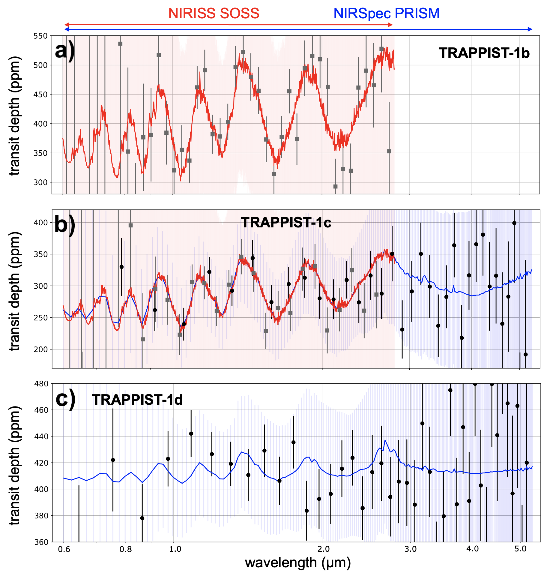
Figure 18: Transit spectra computed for the three innermost planets of the TRAPPIST-1 system calculated from 3D GCM simulations, assuming a 10 bar H₂O atmosphere (+1 bar N₂). Red and blue spectra are calculated for the wavelength coverage of NIRISS SOSS and NIRSpec PRISM, respectively. 1-$\sigma$ error bars are calculated using the JWST Cycle 1 observation program (more details in Section-3.5.2). The transit spectra are in transit depth units (the transit depth is equal to zero at the surface).

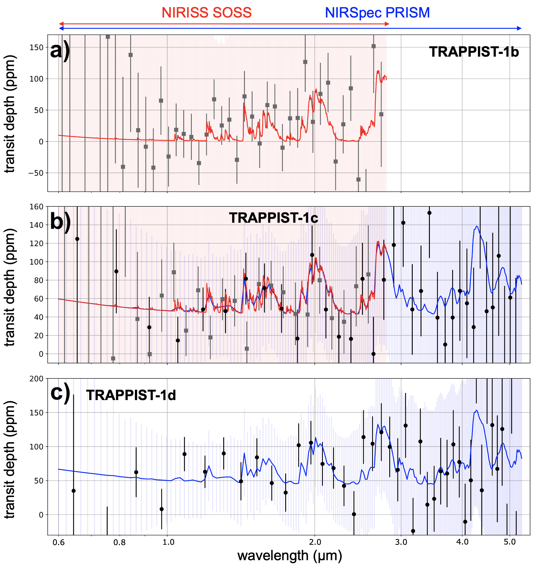
Figure 19: Same as Fig. 18, for 10 bar CO₂ atmospheres.

B.2 Emission spectra and thermal phase curves of TRAPPIST-1b, c and d

We provide here additional figures of emission spectra and thermal phase curves, for each individual GCM simulation of TRAPPIST-1b, c and d. Each plot shows (on the left) the emission spectra at all phase angles ; and (on the right) the associated thermal phase curve, integrated over all wavelengths.

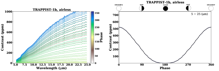
(a)

Figure 22: Thermal emission spectra at various phase angles (left). Thermal phase curve (right) integrated over all wavelengths.

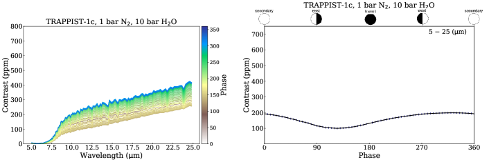
(a)

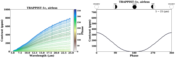
(b)

Figure 23: Thermal emission spectra at various phase angles (left). Thermal phase curve (right) integrated over all wavelengths.

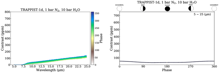
(a)

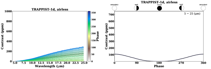
(b)

Figure 25: Thermal emission spectra at various phase angles (left). Thermal phase curve (right) integrated over all wavelengths.

Appendix C The effect of atmospheric expansion

Post-runaway H₂O-dominated atmospheres have been shown to be significantly expanded (Turbet et al. 2019, 2020b). Goldblatt (2015) showed that in extended atmospheres such as H₂O-rich atmospheres, the shortwave (i.e. emitted by the star) and longwave (i.e. emitted by the planet) fluxes can be significantly modified compared to the usual approximation. The absorbed and emitted fluxes are indeed usually calculated by taking the observed radius of the planet as the reference cross-section of the absorbed and emitted in fluxes. To evaluate the error made by this approximation, we have used 1D inverse radiative-convective calculations of H₂O-rich atmospheres (Turbet et al. 2019, 2020b) and calculated for – each spectral band in the radiative transfer – the altitude and therefore the radius at which the opacity is equal to 1. We calculated a shortwave radius $R_{\text{SW}}$ (and a longwave radius $R_{\text{LW}}$) by weighting the spectral radius by the stellar spectrum (and the OTR spectrum, respectively). Fig. 27 shows the scaling factor ratio as a function of surface temperature of the H₂O-rich atmosphere. The scaling factor ratio is defined as $(\frac{R_{\text{LW}}}{R_{\text{SW}}})^{2}$ and provides an estimate of the error made on the TOA radiative budget. There are three important points to notice:

1. The scaling factor ratio is always close (and within a few $\%$) to 1. This indicates that this expansion effect affects the water condensation limit to a few $\%$ as well. The scaling factor ratio being almost always $\geq$ 1, this indicates that the ISR of the water condensation limit was slightly underestimated in our calculations.

2. The evolution of the scaling factor as a function of surface temperature is more sophisticated here than what was calculated in Goldblatt (2015). This is because we calculated the $\tau$ = 1 radius for each spectral band of the model, while Goldblatt (2015) calculated the radius of a wavelength-integrated $\tau$ = 1. As a result, and unlike what Goldblatt (2015) calculated, the scaling factor ratio evolves non-monotonically as a function of surface temperature. At low surface temperatures, the scaling factor ratio increases because $R_{\text{LW}}$ increases much faster (the emission comes from a given atmospheric pressure as shown in Boukrouche et al. 2021, so increasing the total atmospheric pressure increases $R_{\text{LW}}$) than $R_{\text{SW}}$ (the stellar flux always reaches the surface). At intermediate surface temperatures, the scaling factor ratio reaches a plateau, because most of the shortwave flux (and longwave flux) are directly absorbed (and emitted, respectively) by the atmosphere. Increasing the total surface pressure shifts equally $R_{\text{LW}}$) and $R_{\text{SW}}$). At high surface temperatures, the scaling factor ratio decreases. This is because the surface is hot enough that it starts to emit in the visible atmospheric windows of H₂O.

3. The scaling factor varies significantly depending on the total water vapor pressure assumed, as well as the type of host star. This is well illustrated in Fig. 27. Note however that the behaviour of the scaling factor ratio as a function of surface temperature is qualitatively similar for all the cases we explored.

It is important to note however that Fig. 27 likely overestimates the effect of the atmospheric expansion on the TOA radiative budget. This is because we used in this calculation vertical thermal profiles from 1D inverse radiative-convective models, which overestimate temperatures in the low atmosphere, atmospheric scale height and thus atmospheric expansion (Selsis et al. 2023). When high water contents are reached, the temperature profile in the lower atmosphere reaches an isotherm (see e.g. Fig. 13c) thus limiting the atmospheric expansion and the effect on the TOA radiative budget.

Overall, the effect of atmospheric expansion is expected to play a minor role on our calculations of the Water Condensation Zone.

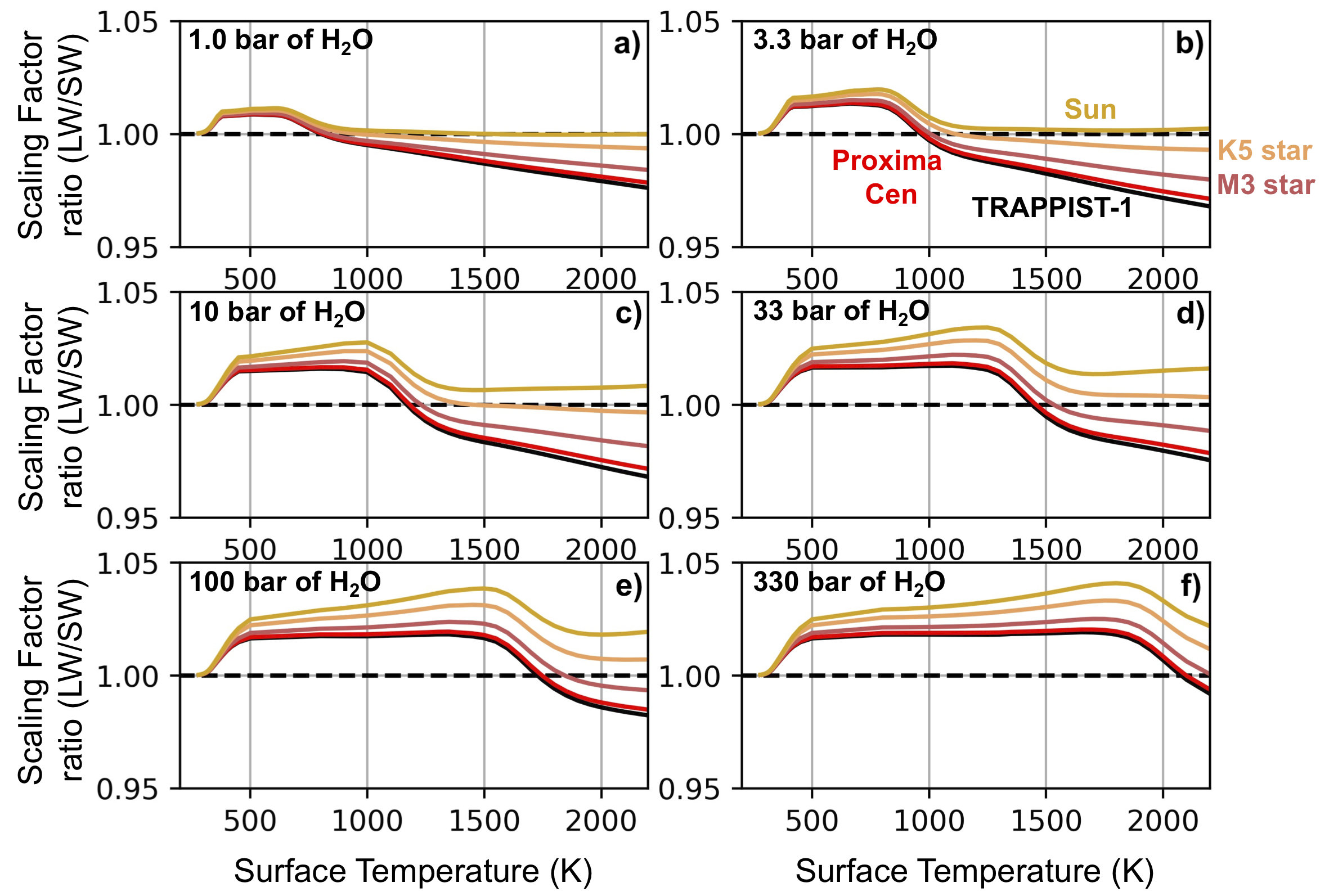
Figure 27: Scaling factor ratio $(\frac{R_{\text{LW}}}{R_{\text{SW}}})^{2}$ as a function of surface temperature, with $R_{\text{LW}}$ the mean planetary radius at which the OTR is emitted ; and $R_{\text{SW}}$ the mean planetary radius at which the ISR is absorbed. Each panel corresponds to a given water content (from 1 to 330 bar of H₂O). The five colors correspond to the five different host stars.

References

- Abe (1997) Abe, Y. 1997, Physics of the Earth and Planetary Interiors, 100, 27
- Abe & Matsui (1988) Abe, Y. & Matsui, T. 1988, Journal of Atmospheric Sciences, 45, 3081
- Agol et al. (2021) Agol, E., Dorn, C., Grimm, S. L., et al. 2021, The Planetary Science Journal, 2, 1
- Angelo et al. (2017) Angelo, I., Rowe, J. F., Howell, S. B., et al. 2017, AJ, 153, 162
- Anglada-Escudé et al. (2016) Anglada-Escudé, G., Amado, P. J., Barnes, J., et al. 2016, Nature, 536, 437
- Anglada-Escudé et al. (2013) Anglada-Escudé, G., Tuomi, M., Gerlach, E., et al. 2013, A&A, 556, A126
- Astudillo-Defru et al. (2017) Astudillo-Defru, N., Forveille, T., Bonfils, X., et al. 2017, A&A, 602, A88
- Baraffe et al. (2015) Baraffe, I., Homeier, D., Allard, F., & Chabrier, G. 2015, Astronomy Astrophysics, 577, A42
- Bolmont et al. (2016) Bolmont, E., Libert, A.-S., Leconte, J., & Selsis, F. 2016, Astronomy Astrophysics, 591, A106
- Bolmont et al. (2017) Bolmont, E., Selsis, F., Owen, J. E., et al. 2017, Monthly Notices of the Royal Astronomical Society, 464, 3728
- Bonfils et al. (2018a) Bonfils, X., Almenara, J. M., Cloutier, R., et al. 2018a, A&A, 618, A142
- Bonfils et al. (2018b) Bonfils, X., Astudillo-Defru, N., Díaz, R., et al. 2018b, A&A, 613, A25
- Bonfils et al. (2013) Bonfils, X., Delfosse, X., Udry, S., et al. 2013, Astronomy Astrophysics, 549, A109
- Borucki et al. (2011) Borucki, W. J., Koch, D. G., Basri, G., et al. 2011, The Astrophysical Journal, 736, 19
- Boucher et al. (1995) Boucher, O., Le Treut, H., & Baker, M. B. 1995, Journal of Geophysical Research, 100, 16
- Boukrouche (2022) Boukrouche, R. 2022, PhD thesis, University of Oxford, Hertford College
- Boukrouche et al. (2021) Boukrouche, R., Lichtenberg, T., & Pierrehumbert, R. T. 2021, The Astrophysical Journal, 919, 130
- Boutle et al. (2020) Boutle, I. A., Joshi, M., Lambert, F. H., et al. 2020, Nature Communications, 11, 2731
- Boutle et al. (2017) Boutle, I. A., Mayne, N. J., Drummond, B., et al. 2017, Astronomy Astrophysics, 601, A120
- Bower et al. (2022) Bower, D. J., Hakim, K., Sossi, P. A., & Sanan, P. 2022, The Planetary Science Journal, 3, 93
- Carone et al. (2014) Carone, L., Keppens, R., & Decin, L. 2014, Monthly Notices of the Royal Astronomical Society, 445, 930
- Carone et al. (2015) Carone, L., Keppens, R., & Decin, L. 2015, Monthly Notices of the Royal Astronomical Society, 453, 2412
- Carone et al. (2016) Carone, L., Keppens, R., & Decin, L. 2016, Monthly Notices of the Royal Astronomical Society, 461, 1981
- Charnay et al. (2021) Charnay, B., Blain, D., Bézard, B., et al. 2021, Astronomy Astrophysics, 646, A171
- Charnay et al. (2015a) Charnay, B., Meadows, V., & Leconte, J. 2015a, The Astrophysical Journal, 813, 15
- Charnay et al. (2015b) Charnay, B., Meadows, V., Misra, A., Leconte, J., & Arney, G. 2015b, The Astrophysical Journal Letters, 813, L1
- Chaverot et al. (2023) Chaverot, G., Bolmont, E., & Turbet, M. 2023, to be submitted to Astronomy & Astrophysics
- Chaverot et al. (2022) Chaverot, G., Turbet, M., Bolmont, E., & Leconte, J. 2022, Astronomy Astrophysics, 658, A40
- Cloutier et al. (2020) Cloutier, R., Eastman, J. D., Rodriguez, J. E., et al. 2020, AJ, 160, 3
- Colose et al. (2021) Colose, C. M., Haqq-Misra, J., Wolf, E. T., et al. 2021, The Astrophysical Journal, 921, 25
- Crossfield et al. (2015) Crossfield, I. J. M., Petigura, E., Schlieder, J. E., et al. 2015, The Astrophysical Journal, 804, 10
- Crossfield et al. (2019) Crossfield, I. J. M., Waalkes, W., Newton, E. R., et al. 2019, ApJ, 883, L16
- Del Genio et al. (2019) Del Genio, A. D., Way, M. J., Amundsen, D. S., et al. 2019, Astrobiology, 19, 99
- Delrez et al. (2022) Delrez, L., Murray, C. A., Pozuelos, F. J., et al. 2022, Astronomy & Astrophysics, 667, A59
- Demory et al. (2020) Demory, B. O., Pozuelos, F. J., Gómez Maqueo Chew, Y., et al. 2020, A&A, 642, A49
- Ding & Wordsworth (2020) Ding, F. & Wordsworth, R. D. 2020, The Astrophysical Journal Letters, 891, L18
- Dransfield et al. (2023) Dransfield, G., Timmermans, M., Triaud, A. H. M. J., et al. 2023, MNRAS[arXiv:2305.06206]
- Dreizler et al. (2020) Dreizler, S., Jeffers, S. V., Rodríguez, E., et al. 2020, MNRAS, 493, 536
- Dressing et al. (2017) Dressing, C. D., Vanderburg, A., Schlieder, J. E., et al. 2017, The Astronomical Journal, 154, 207
- Ducrot et al. (2020) Ducrot, E., Gillon, M., Delrez, L., et al. 2020, Astronomy Astrophysics, 640, A112
- Faria et al. (2022) Faria, J. P., Suárez Mascareño, A., Figueira, P., et al. 2022, Astronomy & Astrophysics, 658, A115
- Fauchez et al. (2021) Fauchez, T. J., Turbet, M., Sergeev, D. E., et al. 2021, The Planetary Science Journal, 2, 106
- Fauchez et al. (2019) Fauchez, T. J., Turbet, M., Villanueva, G. L., et al. 2019, The Astrophysical Journal, 887, 194
- Fauchez et al. (2020) Fauchez, T. J., Turbet, M., Wolf, E. T., et al. 2020, Geoscientific Model Development, 13, 707
- Forget et al. (2013) Forget, F., Wordsworth, R., Millour, E., et al. 2013, Icarus, 222, 81
- Fu & Liou (1992) Fu, Q. & Liou, K. N. 1992, Journal of Atmospheric Sciences, 49, 2139
- Fujii et al. (2017) Fujii, Y., Del Genio, A. D., & Amundsen, D. S. 2017, The Astrophysical Journal, 848, 100
- Gilbert et al. (2020) Gilbert, E. A., Barclay, T., Schlieder, J. E., et al. 2020, The Astronomical Journal, 160, 116
- Gilbert et al. (2023) Gilbert, E. A., Vanderburg, A., Rodriguez, J. E., et al. 2023, The Astrophysical Journal Letters, 944, L35
- Gillon et al. (2017) Gillon, M., Triaud, A. H. M. J., Demory, B.-O., et al. 2017, Nature, 542, 456
- Godolt et al. (2015) Godolt, M., Grenfell, J. L., Hamann-Reinus, A., et al. 2015, Planetary and Space Science, 111, 62
- Goldblatt (2015) Goldblatt, C. 2015, Astrobiology, 15, 362
- Goldblatt et al. (2013) Goldblatt, C., Robinson, T. D., Zahnle, K. J., & Crisp, D. 2013, Nature Geoscience, 6, 661
- Goldblatt & Watson (2012) Goldblatt, C. & Watson, A. J. 2012, Philosophical Transactions of the Royal Society of London Series A, 370, 4197
- Gordon et al. (2022) Gordon, I. E., Rothman, L. S., Hargreaves, R. J., et al. 2022, Journal of Quantitative Spectroscopy and Radiative Transfer, 277, 107949
- Greene et al. (2023) Greene, T. P., Bell, T. J., Ducrot, E., et al. 2023, Nature, 618, 39
- Greene et al. (2017) Greene, T. P., Lagage, P.-O., Rieke, M. J., & Schlawin, E. 2017, MIRI observations of transiting exoplanets, JWST Proposal. Cycle 1, ID. #1177
- Gregory (1995) Gregory, D. 1995, Monthly Weather Review, 123, 2716
- Grimm et al. (2018) Grimm, S. L., Demory, B.-O., Gillon, M., et al. 2018, A&A, 613, A68
- Günther et al. (2019) Günther, M. N., Pozuelos, F. J., Dittmann, J. A., et al. 2019, Nature Astronomy, 3, 1099
- Hamano et al. (2013) Hamano, K., Abe, Y., & Genda, H. 2013, Nature, 497, 607
- Hamano et al. (2015) Hamano, K., Kawahara, H., Abe, Y., Onishi, M., & Hashimoto, G. L. 2015, The Astrophysical Journal, 806, 216
- Harakawa et al. (2022) Harakawa, H., Takarada, T., Kasagi, Y., et al. 2022, PASJ, 74, 904
- Ih et al. (2023) Ih, J., Kempton, E. M. R., Whittaker, E. A., & Lessard, M. 2023, The Astrophysical Journal Letters, 952, L4
- Kaltenegger (2017) Kaltenegger, L. 2017, Annual Review of Astronomy and Astrophysics, 55, 433
- Kane (2022) Kane, S. R. 2022, Nature Astronomy, 6, 420
- Kane et al. (2018) Kane, S. R., Ceja, A. Y., Way, M. J., & Quintana, E. V. 2018, The Astrophysical Journal, 869, 46
- Karman et al. (2019) Karman, T., Gordon, I. E., van der Avoird, A., et al. 2019, Icarus, 328, 160
- Kasting & Harman (2021) Kasting, J. F. & Harman, C. E. 2021, Nature, 598, 259
- Kasting et al. (1993) Kasting, J. F., Whitmire, D. P., & Reynolds, R. T. 1993, Icarus, 101, 108
- Kempton et al. (2018) Kempton, E. M. R., Bean, J. L., Louie, D. R., et al. 2018, PASP, 130, 114401
- Kodama et al. (2015) Kodama, T., Genda, H., Abe, Y., & Zahnle, K. J. 2015, The Astrophysical Journal, 812, 165
- Kodama et al. (2019) Kodama, T., Genda, H., O’ishi, R., Abe-Ouchi, A., & Abe, Y. 2019, Journal of Geophysical Research (Planets), 124, 2306
- Koll (2020) Koll, D. 2020, TLC: Tidally Locked Coordinates, Astrophysics Source Code Library, record ascl:2011.013
- Koll & Abbot (2015) Koll, D. D. B. & Abbot, D. S. 2015, The Astrophysical Journal, 802, 21
- Koll & Cronin (2019) Koll, D. D. B. & Cronin, T. W. 2019, The Astrophysical Journal, 881, 120
- Koll et al. (2019) Koll, D. D. B., Malik, M., Mansfield, M., et al. 2019, The Astrophysical Journal, 886, 140
- Kopparapu et al. (2013) Kopparapu, R. K., Ramirez, R., Kasting, J. F., et al. 2013, The Astrophysical Journal, 765, 131
- Kopparapu et al. (2014) Kopparapu, R. K., Ramirez, R. M., SchottelKotte, J., et al. 2014, The Astrophysical Journal Letters, 787, L29
- Kopparapu et al. (2017) Kopparapu, R. K., Wolf, E. T., Arney, G., et al. 2017, The Astrophysical Journal, 845, 5
- Kopparapu et al. (2016) Kopparapu, R. K., Wolf, E. T., Haqq-Misra, J., et al. 2016, The Astrophysical Journal, 819, 84
- Kossakowski et al. (2023) Kossakowski, D., Kürster, M., Trifonov, T., et al. 2023, A&A, 670, A84
- Kostov et al. (2019) Kostov, V. B., Schlieder, J. E., Barclay, T., et al. 2019, AJ, 158, 32
- Kreidberg et al. (2021) Kreidberg, L., Agol, E., Bolmont, E., et al. 2021, Hot Take on a Cool World: Does Trappist-1c Have an Atmosphere?, JWST Proposal. Cycle 1, ID. #2304
- Lafreniere (2017) Lafreniere, D. 2017, NIRISS Exploration of the Atmospheric diversity of Transiting exoplanets (NEAT), JWST Proposal. Cycle 1, ID. #1201
- Lagage & Bouwman (2017) Lagage, P.-O. & Bouwman, J. 2017, Thermal emission from Trappist1-b, JWST Proposal. Cycle 1, ID. #1279
- Lebrun et al. (2013) Lebrun, T., Massol, H., ChassefièRe, E., et al. 2013, Journal of Geophysical Research (Planets), 118, 1155
- Leconte et al. (2013a) Leconte, J., Forget, F., Charnay, B., Wordsworth, R., & Pottier, A. 2013a, Nature, 504, 268
- Leconte et al. (2013b) Leconte, J., Forget, F., Charnay, B., et al. 2013b, Astronomy.and Astrophysics, in press
- Lichtenberg et al. (2023) Lichtenberg, T., Schaefer, L. K., Nakajima, M., & Fischer, R. A. 2023, in Astronomical Society of the Pacific Conference Series, Vol. 534, Protostars and Planets VII, ed. S. Inutsuka, Y. Aikawa, T. Muto, K. Tomida, & M. Tamura, 907
- Lim et al. (2021) Lim, O., Albert, L., Artigau, E., et al. 2021, Atmospheric reconnaissance of the TRAPPIST-1 planets, JWST Proposal. Cycle 1, ID. #2589
- Lunine (2017) Lunine, J. I. 2017, Acta Astronautica, 131, 123
- Luque & Pallé (2022) Luque, R. & Pallé, E. 2022, Science, 377, 1211
- Lustig-Yaeger et al. (2019) Lustig-Yaeger, J., Meadows, V. S., & Lincowski, A. P. 2019, The Astronomical Journal, 158, 27
- Manabe & Wetherald (1967) Manabe, S. & Wetherald, R. T. 1967, Journal of Atmospheric Sciences, 24, 241
- Mann et al. (2019) Mann, A. W., Dupuy, T., Kraus, A. L., et al. 2019, The Astrophysical Journal, 871, 63
- Massie & Hervig (2013) Massie, S. T. & Hervig, M. 2013, Journal of Quantitative Spectroscopy and Radiative Transfer, 130, 373
- Mlawer et al. (2012) Mlawer, E. J., Payne, V. H., Moncet, J.-L., et al. 2012, Philosophical Transactions of the Royal Society of London Series A, 370, 2520
- Moore & Cowan (2020) Moore, K. & Cowan, N. B. 2020, Monthly Notices of the Royal Astronomical Society, 496, 3786
- Morley et al. (2017) Morley, C. V., Kreidberg, L., Rustamkulov, Z., Robinson, T., & Fortney, J. J. 2017, The Astrophysical Journal, 850, 121
- Muirhead et al. (2015) Muirhead, P. S., Mann, A. W., Vanderburg, A., et al. 2015, ApJ, 801, 18
- Nakajima et al. (1992) Nakajima, S., Hayashi, Y.-Y., & Abe, Y. 1992, Journal of Atmospheric Sciences, 49, 2256
- Parmentier et al. (2021) Parmentier, V., Showman, A. P., & Fortney, J. J. 2021, MNRAS, 501, 78
- Pepe et al. (2011) Pepe, F., Lovis, C., Ségransan, D., et al. 2011, A&A, 534, A58
- Peterson et al. (2023) Peterson, M. S., Benneke, B., Collins, K., et al. 2023, Nature, 617, 701
- Piaulet et al. (2023) Piaulet, C., Benneke, B., Almenara, J. M., et al. 2023, Nature Astronomy, 7, 206
- Rackham et al. (2018) Rackham, B. V., Apai, D., & Giampapa, M. S. 2018, The Astrophysical Journal, 853, 122
- Rackham et al. (2023) Rackham, B. V., Espinoza, N., Berdyugina, S. V., et al. 2023, RAS Techniques and Instruments, 2, 148
- Ramirez & Kaltenegger (2014) Ramirez, R. M. & Kaltenegger, L. 2014, The Astrophysical Journal Letters, 797, L25
- Ramirez & Kaltenegger (2016) Ramirez, R. M. & Kaltenegger, L. 2016, The Astrophysical Journal, 823, 6
- Ramirez & Kaltenegger (2017) Ramirez, R. M. & Kaltenegger, L. 2017, The Astrophysical Journal Letters, 837, L4
- Ramirez & Kaltenegger (2018) Ramirez, R. M. & Kaltenegger, L. 2018, The Astrophysical Journal, 858, 72
- Rathcke et al. (2021) Rathcke, A., Bello-Arufe, A., Buchhave, L. A., et al. 2021, Probing the Terrestrial Planet TRAPPIST-1c for the Presence of an Atmosphere, JWST Proposal. Cycle 1, ID. #2420
- Rossow (1978) Rossow, W. B. 1978, Icarus, 36, 1
- Rowe et al. (2014) Rowe, J. F., Bryson, S. T., Marcy, G. W., et al. 2014, ApJ, 784, 45
- Salvador et al. (2017) Salvador, A., Massol, H., Davaille, A., et al. 2017, Journal of Geophysical Research (Planets), 122, 1458
- Selsis et al. (2023) Selsis, F., Leconte, J., Turbet, M., Chaverot, G., & Bolmont, E. 2023, Nature, 620, 287–291
- Sergeev et al. (2022) Sergeev, D. E., Fauchez, T. J., Turbet, M., et al. 2022, The Planetary Science Journal, 3, 212
- Sergeev et al. (2020) Sergeev, D. E., Lambert, F. H., Mayne, N. J., et al. 2020, The Astrophysical Journal, 894, 84
- Shields et al. (2016) Shields, A. L., Ballard, S., & Johnson, J. A. 2016, Physics Reports, 663, 1
- Shields et al. (2013) Shields, A. L., Meadows, V. S., Bitz, C. M., et al. 2013, Astrobiology, 13, 715
- Suárez Mascareño et al. (2023) Suárez Mascareño, A., González-Álvarez, E., Zapatero Osorio, M. R., et al. 2023, A&A, 670, A5
- Tan et al. (2021) Tan, X., Lefèvre, M., & Pierrehumbert, R. T. 2021, The Astrophysical Journal Letters, 923, L15
- Torres et al. (2017) Torres, G., Kane, S. R., Rowe, J. F., et al. 2017, AJ, 154, 264
- Torres et al. (2015) Torres, G., Kipping, D. M., Fressin, F., et al. 2015, ApJ, 800, 99
- Tuomi et al. (2013) Tuomi, M., Jones, H. R. A., Jenkins, J. S., et al. 2013, A&A, 551, A79
- Turbet (2018) Turbet, M. 2018, Theses, Sorbonne Université / Université Pierre et Marie Curie - Paris VI
- Turbet et al. (2020a) Turbet, M., Bolmont, E., Bourrier, V., et al. 2020a, Space Science Reviews, 216, 100
- Turbet et al. (2021) Turbet, M., Bolmont, E., Chaverot, G., et al. 2021, Nature, 598, 276
- Turbet et al. (2020b) Turbet, M., Bolmont, E., Ehrenreich, D., et al. 2020b, Astronomy & Astrophysics, 638, A41
- Turbet et al. (2018) Turbet, M., Bolmont, E., Leconte, J., et al. 2018, Astronomy Astrophysics, 612, A86
- Turbet et al. (2019) Turbet, M., Ehrenreich, D., Lovis, C., Bolmont, E., & Fauchez, T. 2019, Astronomy & Astrophysics, 628, A12
- Turbet et al. (2017) Turbet, M., Forget, F., Leconte, J., Charnay, B., & Tobie, G. 2017, Earth and Planetary Science Letters, 476, 11
- Turbet et al. (2020c) Turbet, M., Gillmann, C., Forget, F., et al. 2020c, Icarus, 335, 113419
- Turbet et al. (2016) Turbet, M., Leconte, J., Selsis, F., et al. 2016, Astronomy Astrophysics, 596, A112
- Turbet & Selsis (2023) Turbet, M. & Selsis, F. 2023, in Star-Planet Interactions, ed. L. Bigot, J. Bouvier, Y. Lebreton, A. Chiavassa, & A. Lèbre, 202
- Vanderburg et al. (2020) Vanderburg, A., Rowden, P., Bryson, S., et al. 2020, ApJ, 893, L27
- Villanueva et al. (2022) Villanueva, G. L., Liuzzi, G., Faggi, S., et al. 2022, Fundamentals of the Planetary Spectrum Generator
- Villanueva et al. (2018) Villanueva, G. L., Smith, M. D., Protopapa, S., Faggi, S., & Mandell, A. M. 2018, Journal of Quantitative Spectroscopy and Radiative Transfer, 217, 86
- Way & Del Genio (2020) Way, M. J. & Del Genio, A. D. 2020, Journal of Geophysical Research (Planets), 125, e06276
- Way et al. (2018) Way, M. J., Del Genio, A. D., Aleinov, I., et al. 2018, The Astrophysical Journal Supplement Series, 239, 24
- Way et al. (2016) Way, M. J., Del Genio, A. D., Kiang, N. Y., et al. 2016, Geophysical Research Letters, 43, 8376
- Wolf (2017) Wolf, E. T. 2017, The Astrophysical Journal Letters, 839, L1
- Wolf et al. (2020) Wolf, E. T., Haqq-Misra, J., Kopparapu, R., et al. 2020, Journal of Geophysical Research (Planets), 125, e06576
- Wolf et al. (2019) Wolf, E. T., Kopparapu, R. K., & Haqq-Misra, J. 2019, The Astrophysical Journal, 877, 35
- Wolf et al. (2017) Wolf, E. T., Shields, A. L., Kopparapu, R. K., Haqq-Misra, J., & Toon, O. B. 2017, The Astrophysical Journal, 837, 107
- Wolf & Toon (2015) Wolf, E. T. & Toon, O. B. 2015, Journal of Geophysical Research (Atmospheres), 120, 5775
- Wordsworth et al. (2011) Wordsworth, R. D., Forget, F., Selsis, F., et al. 2011, The Astrophysical Journal Letters, 733, L48
- Wunderlich et al. (2019) Wunderlich, F., Godolt, M., Grenfell, J. L., et al. 2019, Astronomy & Astrophysics, 624, A49
- Yang et al. (2019a) Yang, J., Abbot, D. S., Koll, D. D. B., Hu, Y., & Showman, A. P. 2019a, The Astrophysical Journal, 871, 29
- Yang et al. (2014) Yang, J., Boué, G., Fabrycky, D. C., & Abbot, D. S. 2014, The Astrophysical Journal Letters, 787, L2
- Yang et al. (2013) Yang, J., Cowan, N. B., & Abbot, D. S. 2013, The Astrophysical Journal Letters, 771, L45
- Yang et al. (2016) Yang, J., Leconte, J., Wolf, E. T., et al. 2016, The Astrophysical Journal, 826, 222
- Yang et al. (2019b) Yang, J., Leconte, J., Wolf, E. T., et al. 2019b, The Astrophysical Journal, 875, 46
- Zahnle & Catling (2017) Zahnle, K. J. & Catling, D. C. 2017, The Astrophysical Journal, 843, 122
- Zahnle et al. (1988) Zahnle, K. J., Kasting, J. F., & Pollack, J. B. 1988, Icarus, 74, 62
- Zechmeister et al. (2019) Zechmeister, M., Dreizler, S., Ribas, I., et al. 2019, Astronomy & Astrophysics, 627, A49
- Zhang & Showman (2017) Zhang, X. & Showman, A. P. 2017, The Astrophysical Journal, 836, 73
- Zieba et al. (2023) Zieba, S., L., K., Ducrot, E., et al. 2023, Nature