The Agricultural Spraying Vehicle Routing Problem With Splittable Edge Demands

Abstract

In horticulture, spraying applications occur multiple times throughout any crop year. This paper presents a splittable agricultural chemical sprayed vehicle routing problem and formulates it as a mixed integer linear program. The main difference from the classical capacitated arc routing problem (CARP) is that our problem allows us to split the demand on a single demand edge amongst robotics sprayers. We are using theoretical insights about the optimal solution structure to improve the formulation and provide two different formulations of the splittable capacitated arc routing problem (SCARP), a basic spray formulation and a large edge demands formulation for large edge demands problems. This study presents solution methods consisting of lazy constraints, symmetry elimination constraints, and a heuristic repair method. Computational experiments on a set of valuable data based on the properties of real-world agricultural orchard fields reveal that the proposed methods can solve the SCARP with different properties. We also report computational results on classical benchmark sets from previous CARP literature. The tested results indicated that the SCARP model can provide cheaper solutions in some instances when compared with the classical CARP literature. Besides, the heuristic repair method significantly improves the quality of the solution by decreasing the upper bound when solving large-scale problems.

1 Introduction

1.1 Motivation

Precision agriculture has been implemented to provide low-input, high-efficiency, and sustainable agricultural production. In precision agriculture, automation and robotics have become common practice in planting (Cay et al.,, 2018; Khazimov et al.,, 2018; Shi et al.,, 2019), inspection (Mahajan et al.,, 2015; Singh et al.,, 2017; Ozguven et al.,, 2019), spraying (Oberti er al.,, 2016; Vakilian et al.,, 2017; Gonzalez-de-Soto et al.,, 2016), and harvesting (Xiong et al.,, 2019; Williams et al.,, 2019; Barth et al.,, 2016) to overcome the labour shortcomings and improve efficiency (Mahmud et al.,, 2020).

Spraying applications are one of the most critical sectors of agricultural areas. Recently, autonomous agricultural robotic sprayers have been employed in agricultural lands to perform spraying applications such as spraying pesticides, herbicides, and fungicides. Robotic sprayers are a sustainable and human-friendly way to perform spraying operations in orchards. Moreover, as the scale of the orchard increases, the required time frame for spraying operations remains the same. As a result, it is unimaginable to perform the spaying applications only by human workers in a limited time for a large size orchard. Therefore, robotic sprayers have become a more and more popular way to achieve spraying operations in orchard areas.

Finding an optimal routing plan for robotic sprayers is one of the main work in spraying operations. Optimizing the route plan of a robotic sprayer has many benefits, such as reducing time and overall cost, requiring fewer workers, and thus increasing profits (Xu et al.,, 2022).

This paper presents a mixed integer programming-based optimization model for an orchard robotic sprayer routing problem. We give two formulations for the optimization model: the first formulation is a basic spray formulation, and the second is a large edge demands formulation. Our problem allows for multiple robots to satisfy the demand of a row by splitting the spray load. This leads to more efficient utilisation of the tank capacity of the robotic sprayer. We will show that this can provide a cheaper solution than the case where sprayers are required to always process complete rows. We aimed to optimize the path taken by the automatic sprayer to reduce the number of chemicals sprayed while maintaining their effectiveness.

1.2 Problem definition

The classical capacitated arc routing problems (CARP) aim to find minimum-cost paths for a fleet of identical vehicles of capacity P that must service the demand of a subset of edges in a graph. The CARP consists of finding a set of vehicle trips that must satisfy: 1) each vehicle departs from the depot, services a subset of the required edges, and returns to the depot; 2) the total demand serviced by a vehicle does not exceed P; 3) each required edge is serviced by exactly one vehicle. The CARP model is a good starting point as an abstraction of our problem, where vehicles are spraying robots and the arcs to be serviced are rows of an orchard, with demand of an arc being the amount of liquid that has to be sprayed in that row. However, the requirement that only a single vehicle must serve a whole arc seems unnecessarily restrictive. This paper solves an extension of CARP, which allows splitting the demand on a single demand edge amongst robots.

This paper presents a splittable capacitated arc routing problem (SCARP) for orchards. The real-world orchard’s shape, tractor tracks, barrier blocks, and tracks connecting the barriers form the graph of the orchard. An orchard is represented as an undirected graph $\mathcal{G}$. The tractor tracks are the lines on the graph $\mathcal{G}$. In graph theory, we call these lines as edges. In practice, some edges that need to be sprayed are demand edges or required edges, with each required edge having a demand, and those without demanding are non-demand edges. Edges in the orchard were classified as headland edges, interior edges, and island edges. In practice, we only need to spray interior edges (for example, dashed lines in Fig. 1). Any intersection between two edges on a graph is vertex. In practice, huge barrier blocks are formed by planted trees and islands that prohibit vehicles from passing. We call these barriers as obstacle areas. Fig. 1 is an example of the small orchards based on the attributes of the real-world examples based on the graphs from  Plessen et al., (2019). Fig. 1 provides two main types of orchard graphs: uninterrupted (no obstacles) and interrupted graphs. The dots are vertices, whereas the solid, dashed, and dash-dotted lines represent the headland, interior, and island edges. In this problem, all robots start from a fixed depot (for example, vertex $1$ is a depot in Fig. 1). The robot does spraying work subject to the robot’s capacity and edge demands of this orchard. Every required edge must be sprayed by at least one robotic sprayer. The robotic sprayers are refilled at the depot when they run out of chemicals to spray. It is worth noting that this problem could be seen as both a multi-robotic and single-robotic spraying routing problem.

In summary, the properties of the graph and robot sprayer of SCARP are:

1. Arbitrarily shaped orchards (convex or non-convex)

2. Availability of a transition graph with edges connecting vertices

3. A corresponding non-negative cost array with edge costs equal to the path length of edges

4. Corresponding non-negative edge demands (Edge demand should be non-zero for those edges that must be sprayed)

5. A fixed robotics capacity. The total demand serviced by a robot does not exceed the capacity

6. A designated start vertex (depot), same start and end vertex

7. Fix the depot (refilled position) at the start vertex, and if the robot runs out of liquid to spray, it goes back to refill

8. The demand of one edge may be satisfied by more than one robot (split demand)

9. There is a single robotic sprayer by default

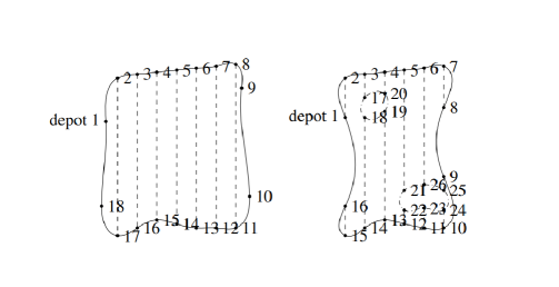
Figure 1: An example of the small orchards based on the attributes of the real-world examples (Plessen et al.,, 2019): solid, dashed, and dash-dotted lines denote the headland, interior, and island edges. Dots indicate the vertices. (Left) Uninterrupted edges when aligned in a rotated coordinated frame. (Right) Interrupted edges due to orchard field indentations and obstacle areas prohibit the passage of any vehicle operating in the orchard. We set vertex 1 as the depot, and robotic sprayers depart from the depot and spray the interior edges (dashed line). If the robotic sprayers run out of chemicals, it goes back to the depot to refill.

The SCARP is an NP-hard problem, since it can be reduced to the NP-hard Rural Postman Problem (RPP) (Lenstra et al.,, 1976) by giving the robot an unlimited capacity. This study presents solution methods consisting of lazy constraints, symmetry elimination constraints, and a heuristic repair method. We tested our algorithm on valuable data sets based on a real-world problem and a set of classical instances from CARP literature. This research proposes several contributions to developing an agricultural robot performing spraying tasks autonomously and gives some inspiration for mobile routing problems.

The remaining paper is organized as follows: A brief review of the relevant literature is given in the Section 2. Next, we provide a mathematical formulation of the SCARP in Section 3. After that, we analyze the properties of the SCARP in Section 4. The solution strategy is given in Section 5. In addition, we reveal the success of the algorithms in Section 6. Then, Section 7 shows the parameter analysis of the heuristic repair method. Finally, we conclude the paper and point out the future research directions in Section 8.

2 Literature review

Optimizing logistics and route planning plays a vital role in the agricultural area. The minimum navigation cost by finding the shortest path in mobile robot navigation could provide a convenient service with the lowest cost to the farmers.

A capacitated variation of Vehicle Routing Problem (VRP) is known as the Capacitated Vehicle Routing Problem (CVRP) (Braekers et al.,, 2016). The CVRP seeks total cost-minimizing routes for multiple identical vehicles with limited capacity and where multiple vertices (customers) subject to various demands must be serviced exactly once by exactly one vehicle (Laporte et al.,, 1992). Archetti et al., (2012) propose the Split Delivery Vehicle Routing Problem (SDVRP), where each customer may be served by multiple vehicles. The VRPs are computationally expensive and categorized as NP-hard (Lenstra et al.,, 1981). There are many variations (Lysgaard et al.,, 2020; Chiang et al.,, 2014; Toth et al.,, 2014; Laporte et al.,, 1992). The well-known Traveling Salesman Problem (TSP) (Grötschel et al.,, 1985) is a particular case of the VRP when only one vehicle is available at the depot, and no additional operational constraints are imposed. Numerous applications exist that involve integrating VRP with other problems, such as combining it with the depot location problem to construct a Location Routing Problem (LRP) (Quintero-Araujo et al.,, 2017). In contrast to the robotics spraying agricultural routing problem focus on edge-coverage, the VRPs typically vertex-coverage is of primary importance. Therefore, instead of VRPs, arc routing problems (ARPs) are here of more interest.

In Arc Routing Problem (ARP), the customers are located not at the vertices but along the arcs of the road network, are described in the book edited by Dror et al., (2012). There are many real-life applications of ARP such as garbage collection (Amponsah et al.,, 2004), postal delivery (Eiselt et al., 1995, a, b), snow removal (Campbell et al.,, 2000) and others. Monroy-Licht et al., (2017) introduce a dynamic ARP that addresses disruptions caused by vehicle failure in the incapacitated case. For ARPs, problems can be distinguished between the classes of the Chinese Postman Problem (CPP) and the Rural Postman Problem (RPP), where all and only a subset of all arcs of the graph need to be traversed, respectively (Eiselt et al., 1995, a, b). However, neither the CPP nor the RPP considers the vehicle’s capacity or the edge demands.

The Capacitated Arc Routing Problem (CARP) was formally introduced by Golden et al., (1981). This important problem plays the same role in arc routing as the CVRP in node routing. Roughly speaking, the CARP consists of finding a set of minimum-cost routes for vehicles with limited capacity that service some street segments with known demand, represented by a subset of edges of a graph. The CARP is an NP-hard problem. Golden et al., (1981) showed that even the 0.5 approximate CARP is NP-hard. Besides, finding a feasible solution for the CARP that uses a given number of vehicles is also NP-hard. Thus, the CARP is considered to be very difficult to solve exactly. The SCARP can be seen as a relaxation problem of the classical CARP. The difference between the CARP and the SCARP in this paper is that, in SCARP, the demand for a single edge may be satisfied by more than one vehicle.

Benavent et al., (1992) developed a dynamic programming-based technique to compute lower bounds to the CARP with a fixed number of vehicles and generated a set of network instances for the CARP. Our research also works on a fixed precomputed number of vehicles, and we provide a comparison result with these Benavent’s instances set. Some authors have solved the CARP by transforming it into a capacitated node routing problem (Baldacci et al.,, 2006), which applies an exact algorithm to compute the lower bounds of the CARP. Belenguer et al., (2015) classified exact methods into three groups: branch-and-bound based on combinatorial lower bounds, cutting-plane and branch-and-cut, column-generation and branch-and-price methods. Belenguer et al., (2003) introduced some new valid inequalities for the CARP and implemented a cutting plane algorithm for this problem. However, increasing the lower bounds significantly for large-scale problems by exact methods is difficult. Moreover, exact methods are limited to moderated instances (Chen et al.,, 2016). Several heuristic algorithms have been developed for the CARP, such as simulated annealing algorithm (Eglese et al.,, 1994), tabu search heuristic (Hertz et al.,, 2000), improved ant colony optimization based algorithm (Santos et al.,, 2010), etc. Lacomme et al., (2004) proposed memetic algorithms (MAs), which provided a better solution in some classical instance sets for solving an extended CARP. This paper provides a heuristic repair method to decrease the upper bounds for SCARP, which could provide cheaper solutions in some large-scale CARP instances.

In this paper, we present a SCARP problem and formulate it as a mixed integer linear program. We are using theoretical insights about the optimal solution structure to improve the solutions. We implement lazy constraints, symmetry elimination constraints, and heuristic repair method to solve the SCARP. Computational experiments show that the SCARP model can provide cheaper solutions in some instances when compared with the classical CARP literature. Besides, the heuristic repair method significantly improves the quality of the solution by decreasing the upper bound when solving large-scale problems.

3 Mathematical formulations

3.1 Nomenclature

• Sets

  • $\mathcal{V}=\{1,2,...,n\}$ set of all vertices;

  • $\mathcal{E}=\{(i,j):i,j\in\mathcal{V},\ i\neq j\}$ set of all existing directed arcs of this graph. When the distance from $i$ to $j$ is not zero, it means this arc exists;

  • $\mathcal{U}=\{(i,j)\in\mathcal{E}:i<j\}$ set of undirected arcs (set of arcs, when not need to consider the direction).

  • $\mathcal{G=(V,U)}$ an undirected connected graph;

  • $\mathcal{I}_{k}=\{i\in\mathcal{E}:(i,k)\in\mathcal{E}\}$ set of incoming arcs of vertex $k$;

  • $\mathcal{Q}_{k}=\{j\in\mathcal{E}:(k,j)\in\mathcal{E}\}$ set of outgoing arcs of vertex $k$;

  • $\mathcal{R}=\{1,2,...,r\}$ set of the index of the robotic sprayer’s tour for single robotic sprayer problem or robotic sprayer for multiple robotic sprayers problem. $r$ equals the smallest integer greater than the total demand divide the capacity of the robot sprayer $r=\frac{\sum_{(i,j)\in\mathcal{V}}D_{ij}}{P}$. We can refer to it as robot to simplify.

• Parameters

  • $C_{ij}$ non-negative cost (km) of arc $(i,j)\in\mathcal{U}$;

  • $D_{ij}$ non-negative demand of spray (L) of arc $(i,j)\in\mathcal{U}$;

  • $P$ robot sprayer capacity (L);

  • fixed depot is vertex 1 by default.

• Decision variables

  • $x_{ij}^{r}$ a binary variable, which is 1 if the arc $(i,j)\in\mathcal{E}$ is traversed by $r\in\mathcal{R}$, 0 otherwise;

  • $y_{ij}^{r}$ the amount of chemicals sprayed of edge $(i,j)\in\mathcal{U}$ with robot $r\in\mathcal{R}$. Fix $y_{ij}^{r}=0$ if $D_{ij}=0$.

3.2 SCARP formulation 1: Basic robotic spraying formulation

$$\underset{\displaystyle}{\mathrm{min}}\quad\sum_{r\in\mathcal{R}}\sum_{(i,j)\in\mathcal{U}}C_{ij}(x_{ij}^{r}+x_{ji}^{r})\quad(j,i)\in\mathcal{E}$$ (1a)

$$\mathmakebox[\widthof{$\underset{\displaystyle\phantom{}}{\mathrm{min}}$}][c]{\mathmakebox[\widthof{$\mathrm{min}$}][l]{\mathrm{\kern 1.00006pts.t.}}}$$

$$\sum_{(i,j)\in\mathcal{U}}y_{ij}^{r} \leq P \quad\forall\ r\in\mathcal{R}$$ (1b)

$$y_{ij}^{r} \geq 0 \quad\forall\ (i,j)\in\mathcal{U},\ r\in\mathcal{R}$$ (1c)

$$\sum_{r\in\mathcal{R}}y_{ij}^{r} =D_{ij} \quad\forall\ (i,j)\in\mathcal{U}$$ (1d)

$$y_{ij}^{r} \leq P(x_{ij}^{r}+x_{ji}^{r}) \quad\forall\ (i,j)\in\mathcal{U},\ r\in\mathcal{R}$$ (1e)

$$\sum_{i\in\mathcal{I}_{k}}x_{ik}^{r} =\sum_{j\in\mathcal{Q}_{k}}x_{kj}^{r} \quad\forall\ k\in\mathcal{V},\ r\in\mathcal{R}$$ (1f)

$$\sum_{i\in\mathcal{S},j\in\mathcal{T}}Px_{ij}^{r} \geq\sum_{i,j\in\mathcal{T}}y_{ij}^{r} \ \ \begin{array}[]{l@{}l}\forall&\ \mathcal{S}\subset\mathcal{V},\ 1\in\mathcal{S},\\ &\mathcal{T}=\mathcal{V}\setminus\mathcal{S},\ r\in\mathcal{R}\end{array}$$ (1i)

$$x_{ij}^{r} \in\{0,1\} \quad\forall\ (i,j)\in\mathcal{E},\ r\in\mathcal{R}$$ (1j)

The objective function (1a) seeks to minimize the total distance travelled. Constraints (1b) state the total sprays of a robot do not exceed the robot’s capacity. Constraints (1c) confirm the number of sprays on each edge are greater than or equal to 0. Constraints (1d) ensure the total amount of sprays on each edge equal the corresponding edge demands. Constraints (1e) guarantee that the edge $(i,j)$ can be sprayed by a robot only if the robot covers edge $(i,j)$ with robot $r$ (robot $r$ can serve edge $(i,j)$ in both directions). Constraints (1f) are flow conservation constraints for each vertex, which assure route continuity. Constraints (1i) enforce that any set of vertices $\mathcal{T}$ that contains arcs are sprayed by a robot $r$ ($y_{ij}^{r}>0$) must be reachable by the robot from the other side of the cut that contains the depot (set $\mathcal{S}$). Integrality restrictions are given in Constraints (1j).

4 Properties of the SCARP

4.1 Properties

In addition to the notation already introduced, we make the following definitions and provide the relevant properties of the SCARP.

Definition 1.

The support of a robot in a solution is the set of edges where the robot satisfies the demand $S_{r}(y)=\{(i,j)\in\mathcal{U},\ y^{r}_{ij}>0\}$ For any solution $x,y$ we can group robots into categories based on the size of the support:

$$R_{0}(y)=\{r:S_{r}(y)=\emptyset\}=\text{unused robots}$$

$$R_{1}(y)=\{r:\lvert S_{r}(y)\rvert=1\}=\text{robots spraying a single edge}$$

$$R_{2+}(y)=\{r:\lvert S_{r}(y)\rvert\geq 2\}=\text{robots spraying multiple edges}$$

Theorem 1.

For any robotic sprayer routing problem, there exists an optimal solution $x,y$ such that $\lvert R_{2+}(y)\rvert<m=\lvert\mathcal{U}\rvert$ that is less than $m$ robots spray multiple edges; all the remaining robots are either unused or have singleton support (spray a single edge).

Proof.

Assume there exists an optimal solution $x,y$ with $\lvert R_{2+}(y)\rvert\geq m$. $x$ is the set of decision variables $x_{ij}^{r}$, whereas $y$ is the set of actual chemical sprays $y_{ij}^{r}$. Transfer the edge to the vertex to construct an auxiliary graph. More specifically, the vertices of the auxiliary graph are the edges of the original graph, and there exists a link in the auxiliary graph if the original two edges share the same vertices. Then there are at least $m$ robots covering multiple edges, meaning the auxiliary graph has at least $m$ vertices and $m$ edges. Thus the auxiliary graph exists in at least one cycle. Fig. 2 give an example to illustrate the proof idea.
Step 1: There are greater than or equal to $m$ edges in the auxiliary graph, identify a cycle $C$.
Step 2: Balancing spray around cycle $C$, update the solution by an amount sufficient to ensure one vertex in the auxiliary graph has spray 0. Note that for a cycle, every vertex visited by the cycle has exactly two adjacent edges. The divergence of the vertices equals $0$. In other words, if increase the sprays of an edge from the original graph of robot $r$, the sprays of the same edge from another robot will decline. Considering the vertices in the auxiliary graph and cycles, either of the following will happen.

Case 1:

There exists an edge $(i,j)$ for which demand of spray is greater than or equal to $P$. Increasing the chemical sprays $y^{r}_{ij}$ = $P$, decreasing the remaining vertices sprays to $0$, and adjusting the sprays of other vertices to maintain the balance of capacity of robot $r$ and chemical demands of the vertex in the auxiliary graph.

Case 2:

Otherwise, increase the chemical sprays of a vertex to the required edge demands and decrease the same vertex sprays to $0$ for the other robots. Finally, adjust the sprays of other vertices to maintain the balance of the robot’s capacity and the vertex’s required demands.

Step 3: Remove edges with zero sprays in the updated solution.
Step 4: Cycle $C$ does not exist. If there are greater than or equal to $m$ edges in the auxiliary graph, go to Step $1$.
Step 5: Updating the auxiliary graph find $\bar{y}$ (updated solution of set $y$) satisfied $\lvert R_{2+}(\bar{y})\rvert<\lvert R_{2+}(y)\rvert$.

We get a new solution $(x,\bar{y})$ with fewer robots spraying multiple edges. In conclusion, there exists an optimal solution with less than $m$ robots spraying multiple edges. ∎

(a) Original graph

(b) Auxiliary graph

(c) Updated graph

Figure 2: Give an example to illustrate the proof idea of  Theorem 1. $A$ to $G$ are edge demands, and $1$ to $6$ are vertices. $\{r_{1},r_{2},...,r_{7}\}$ are multi-robotic tours. Transfer the edges of the original graph to the vertices to construct an auxiliary graph. More specifically, the vertices of the auxiliary graph are the edges of the original graph, and there exists a link in the auxiliary graph if the original two edges share the same vertices. We decrease the number of robotics by breaking the cycles in the auxiliary graph. In this example, we break the cycle in Fig. 2(c), and the number of multi-robotic decreases from $7$ to $6$.

Based on the above theorem, we might hope to reduce the size of the problem further by simply using robot trips that empty their whole capacity on a single row whenever that row has a demand greater than the tank capacity. The next theorem shows that this strategy does not guarantee an optimal solution.

Theorem 2.

For arbitrary robot spray routing problems, the condition $D_{ij}>P$ is not sufficient to guarantee that there exists an optimal solution with a robot $r$ such that $\bar{y}^{r}_{ij}=P$.

Proof.

We prove this by providing a counter-example. Consider the problem in Fig. 3. As shown in the figure, $D_{23}=12$ all other $D_{ij}=1$ and all $C_{ij}=1$. Let $P=8$ then $D_{23}>P$.

Figure 3: Counter-example: An undirected graph and the fixed depot is vertex $1$. A robotic sprayer starts from the depot to spray chemicals to edges (1,2), (1,3), (1,4), (2,3), and (3,4). The number along each edge is the edge corresponding required demands.

Table 1: Optimal solution of the counter-example of  Fig. 3

$r_{1}$	$(1,2)$	$(2,3)$	$(3,1)$
	$y^{r_{1}}_{12}=0$	$y^{r_{1}}_{23}=7$	$y^{r_{1}}_{31}=1$
$r_{2}$	$(1,2)$	$(2,3)$	$(3,4)$	$(4,1)$
	$y^{r_{2}}_{12}=1$	$y^{r_{2}}_{23}=5$	$y^{r_{2}}_{34}=1$	$y^{r_{2}}_{41}=1$

Table 2: New solution of the counter-example of  Fig. 3

$r_{1}$	$(1,2)$	$(2,3)$	$(3,1)$
	$\bar{y}^{r_{1}}_{12}=0$	$\bar{y}^{r_{1}}_{23}=8$	$\bar{y}^{r_{1}}_{31}=0$
$r_{2}$	$(1,2)$	$(2,3)$	$(3,4)$	$(4,1)$	$(1,3)$	$(3,1)$
	$\bar{y}^{r_{2}}_{12}=1$	$\bar{y}^{r_{2}}_{23}=4$	$\bar{y}^{r_{2}}_{34}=1$	$\bar{y}^{r_{2}}_{41}=1$	$\bar{y}^{r_{2}}_{13}=1$	$\bar{y}^{r_{2}}_{31}=0$

Table 1 gives an optimal solution value to SCARP formulation 1 of $7$. Table 2 shows when the first robot is fixed to only spray edge $(2,3)$, the optimal solution cost will be increased to $9$. Thus, for any robot sprayer routing problem, if $D_{ij}>P$ for some $(i,j)\in\mathcal{U}$ and here not always existing an optimal solution $\bar{x},\bar{y}$ and a robot $r$ such that $\bar{y}^{r}_{ij}=P$. ∎

4.2 SCARP formulation 2: large edge demands formulation

Based on Theorem 1 there is an opportunity to create a simpler formulation when some of the edges’ demands $D_{ij}$ are much greater than $P$.

Apply Dijkstra’s algorithm to calculate the shortest path distance from the start vertex $1$ (depot) to other vertices in the graph. Let $SP_{1i}$ be the shortest path distance from vertex $1$ to vertex $i$. $\mathcal{R}_{new}=\{1,2,...,$min$(\lvert\mathcal{U}\rvert-1,\lvert\mathcal{R}\rvert=\frac{\sum_{(i,j)\in\mathcal{U}}D_{ij}}{P})\}$ set of robots that work on multiple edges. $z_{ij}\in\mathbb{Z}_{+}$ the number of singleton robots that spray edge $(i,j)\in\mathcal{U}$.

$$\underset{\displaystyle}{\mathrm{min}}\quad\sum_{(i,j)\in\mathcal{U}}z_{ij}(SP_{1i}+C_{ij}+SP_{j1})+\sum_{r\in\mathcal{R}_{new}}\sum_{(i,j)\in\mathcal{U}}C_{ij}(x_{ij}^{r}+x_{ji}^{r})\quad(j,i)\in\mathcal{E}$$ (2a)

$$\mathmakebox[\widthof{$\underset{\displaystyle\phantom{}}{\mathrm{min}}$}][c]{\mathmakebox[\widthof{$\mathrm{min}$}][l]{\mathrm{\kern 1.00006pts.t.}}}$$

$$\sum_{(i,j)\in\mathcal{U}}y_{ij}^{r} \leq P \quad\forall r\in\mathcal{R}_{new}$$ (2b)

$$y_{ij}^{r} \geq 0 \quad\forall(i,j)\in\mathcal{U},r\in\mathcal{R}_{new}$$ (2c)

$$\sum_{r\in\mathcal{R}}y_{ij}^{r}+z_{ij}P \geq D_{ij} \quad\forall(i,j)\in\mathcal{U}$$ (2d)

$$y_{ij}^{r} \leq P(x_{ij}^{r}+x_{ji}^{r}) \quad\forall(i,j)\in\mathcal{U},r\in\mathcal{R}_{new}$$ (2e)

$$\sum_{i\in\mathcal{I}_{k}}x_{ik}^{r} =\sum_{j\in\mathcal{Q}_{k}}x_{kj}^{r} \quad\forall k\in\mathcal{V},r\in\mathcal{R}_{new}$$ (2f)

$$\sum_{i\in\mathcal{S},j\in\mathcal{T}}Px_{ij}^{r} \geq\sum_{i,j\in\mathcal{T}}y_{ij}^{r} \quad\begin{subarray}{c}\forall\mathcal{S}\subset\mathcal{V},S\cup\mathcal{T}=\mathcal{V},\\ 1\in\mathcal{S}\mathcal{T}=\mathcal{V}\setminus{\mathcal{S}},r\in\mathcal{R}_{new}\end{subarray}$$ (2g)

$$x_{ij}^{r} \in\{0,1\} \quad\forall(i,j)\in\mathcal{E},r\in\mathcal{R}_{new}$$ (2h)

$$z_{ij} \leq\frac{D_{ij}}{P} \quad\forall(i,j)\in\mathcal{U}$$ (2i)

The key idea is splitting the large demand on a single edge amongst vehicles to involve fewer vehicles to decrease the number of decision variables $x^{r}_{ij}$ and $y^{r}_{ij}$ when $\lvert\mathcal{R}\rvert>\lvert\mathcal{U}\rvert-1$. Theorem 1 indicates that there exits at least one robotic sprayer robot $r$ that $\bar{y}^{r}_{ij}=P$ when $\lvert\mathcal{R}\rvert>\lvert\mathcal{U}\rvert-1$. More specifically, there are at most $\lvert\mathcal{U}\rvert-1$ multi-robotic and at least $\lvert\mathcal{R}\rvert-(\lvert\mathcal{U}\rvert-1)$ single-robotic (Except in the case of the last robot covering the rest of the spray). The objective function  (2a) consists of singleton and multi-robotic’ costs. Similarly, Constraints  (2d) indicate each edge can be serviced by singleton and multi-robotic sprayers. Hence, the total edge demand comes from the chemicals sprayed by singleton and multi-robotic sprayers.

5 Methodology

5.1 Lazy-constraints

Lazy constraints are useful when the full set of constraints is too large to include in the initial formulation. The main idea is to remove the costly constraints and get a relaxed problem with the remaining constraints. And then, we reintroduce that constraint if the relaxation solutions violate some of the constraints we left out.

The basic formulation described in Section 3 is costly for a large-scale problem. Because the number of Constraints (1i) grows exponentially as the vertices increase in the graph. We simply cannot afford to list them all for decent size graphs. An alternative is to treat them as lazy constraints and only add them when they are violated.

The main steps for applying lazy constraints are as follows:

• Remove the connectivity Constraints (1i);

• For any LP solution obtained during the branch-and-bound, test if the solution violates Constraints (1i) for any robot $r$. If it does, go to the next step, otherwise, skip the lazy constraints;

• Use the BFS algorithm to generate suitable subset $\mathcal{S}$ of $\mathcal{N}$. Pass the $\mathcal{S}$ to build cuts in the branch-and-bound process.

The constraints could be added at both branch-and-bound nodes with integer and fractional LP solutions. For the sake of computational efficiency, we add constraints for fractional solutions early in the search and all infeasible integer solutions. More specifically, we add lazy constraints on a limited number of nodes (not too deep in the branch and bound tree) when the gap between the lower and upper bound is not too small.

5.2 Symmetry elimination constraints

There are many equivalent ways to encode the same solution in our formulation simply by renumbering the robots. We can eliminate this symmetry with Constraints (3a). The Constraints (3a) order the robots from less costly to more to eliminate symmetric solutions.

$$\sum_{(i,j)\in\mathcal{A}}C_{ij}x_{ij}^{r}\geq\sum_{(i,j)\in\mathcal{A}}C_{ij}x_{ij}^{r-1}\hskip 10.00002pt\forall r\in\mathcal{R}_{new}:r>1$$ (3a)

Another form of symmetry is due to the fact that traversing a route in the reverse order does not change the solution. To eliminate this symmetry, let $N^{i}_{1}=\{i\in(i,1):\forall(i,1)\in\mathcal{I}_{1}\}$ be the set of vertices for arcs coming into start vertex $1$. The Constraints (3b) orients the route by not allowing the return arc at the depot to connect to a lower indexed node than the outgoing arc. However, this doesn’t help if the first and last edge visited by the robot are the same.

$$\sum_{i=1}^{k}x_{1i}^{r}\geq x_{k1}^{r}\hskip 10.00002pt\forall k\in N^{i}_{1},\hskip 5.0pt\forall r\in\mathcal{R}_{new}$$ (3b)

5.3 Heuristic repair method

We provide a heuristic repair method that can be applied to any infeasible (fractional) solutions. The main idea is to construct heuristic solutions based on infeasible solutions and use them as new incumbents during the branch-and-bound.

We detail its main components in the following paragraphs.

Preprocessing step: Compute shortest path and corresponding shortest distance (cost) from vertex $i$ to vertex $j$ ($\forall\ i,j\in\mathcal{V}$) by Dijkstra’s algorithm, represented by $SPath_{ij}$ and $SP_{ij}$, respectively.

Using an infeasible solution with feasible $y$ values to construct a connected path that covers all edges $(i,j)$ such that $y_{ij}^{r}>0$ by the Greedy routing algorithm ($y_{ij}^{r}$ can be fractions, thus they are always feasible). It is worth noting that in chaining paths from one spray edge to the next we may be traversing an arc in the same direction twice and that we can trivially improve the solution by removing such duplicates. Then generate $x_{ij}^{r}$ according to the connected path. At last, sort $x_{ij}^{r}$ and $y_{ij}^{r}$ according to the symmetry elimination constraints in (3a) and (3b).

Data: Infeasible solutions with feasible $y=\{y_{ij}^{r}:(i,j)\in\mathcal{U},r\in\mathcal{R}\}$, $SPath_{ij}$ , $SP_{ij}$

Result: Feasible solutions $x=\{x_{ij}^{r}:(i,j)\in\mathcal{E},r\in\mathcal{R}\}$, $y$;

1 $F\_edge=\{(i,j):y_{ij}^{r}>0\}$;

2 $B\_edge=\{(j,i):y_{ij}^{r}>0\}$;

3 $All\_edge=append!(F\_edge,B\_edge)$;

$s=1$ ;

  $\triangleright$ Depot $\triangleright$ 

4

5 Function Greedy routing($y$, $SPath_{ij}$, $SP_{ij}$):

6       $route=$ Connectable path $(y,SPath_{ij},SP_{ij})$;

7       $path=$ Remove duplicate $(y,SPath_{ij},SP_{ij},route)$;

8       for $(i,j)\in path$ do

9             $x\leftarrow x_{ij}^{r}=1$;

10       end for

11      $order\leftarrow$ 3a, 3b;

12       Sorting $x,y\leftarrow order$;

13       return $x,y$

14 end

15

16 Function Connectable path($y$, $SPath_{ij}$, $SP_{ij}$):

17       $route\leftarrow\emptyset$ ;

18       while $\lvert All\_edge\rvert\neq 0$ do

19             $n\leftarrow$ vertices passed by $F\_edge$ ;

20             $v\leftarrow$ min($SP_{sn}$ , n);

21             if $\lvert SPath_{sv}\rvert\geq 2$ then

22                   $route\leftarrow$ append $SPath_{sv}$;

23             end if

24            $pass\_vertex\leftarrow\{j:(v,j)\in F\_edge\}$;

25             if  $\lvert\text{pass\_vertex}\rvert=0$ then

26                   $reverse\_vertex\leftarrow\{j:(j,v)\in B\_edge\}$;

27                   $pass\_vertex\leftarrow$ append $reverse\_vertex[1]$;

28                  

29             end if

30            $route\leftarrow$append $pass\_vertex[1]$;

31             update $F\_edge$, $B\_edge$ by removing covered edges in both directions;

32             $All\_edge\leftarrow append!(F\_edge,B\_edge)$;

33            

34       end while

35      if route[end] != 1 then

             $back=SPath_{route[end]s}$ ;

              $\triangleright$ find shortest path from $route[end]$ to $s$ $\triangleright$ 

36             $route\leftarrow$append $SPath_{route[end]s}$;

37            

38       end if

39      return $route$

40 end

41 Function Remove duplicate($y$, $SPath_{ij}$, $SP_{ij}$, $route$):

42       for $i\leftarrow 1$ to $\lvert route\rvert-1$  do

43             $path\leftarrow{(route[i],route[i+1])}$;

44       end for

45      if path has duplicated edges then

46             remove duplicated edges from $path$

47       end if

48      return path

49 end

50

Algorithm 1 Greedy routing algorithm

In Alg. 1 Greedy routing function, some edges need to be reversed, such as reversing $(i,j)$ to $(j,i)$ to get a connectable path when the outgoing vertex is $j$. The traversal of $(i,j)$ or $(j,i)$ are both seen as a coverage of $(i,j)$. If it is an edge in $F\_edge$, remove it from $F\_edge$, then swap the edge order and remove it from $B\_edge$, and vice versa.

The heuristic repair method also generates many rejected solutions, which return worse objective values than the exits. To improve the efficiency, we set a parameter $\Gamma$ representing the number of times the heuristic will be run without improvement before abandoning any further attempts to run the repair heuristic. Section 7 provides an analysis of the parameter $\Gamma$.

6 Numerical results

In this section, we test the effectiveness of our algorithms for solving this agricultural vehicle spraying problem. We consider three main classes of instances. The first and second classes of instances are generated by ourselves based on the attributes of the real-world examples described by Plessen et al., (2019).

Table 3: Comparative results of the Basic and the Large edge demands models on the same graph LD with different edge demands. LD consists of 16 vertices and 22 edges, which is displayed in Fig. 5. Robot capacity equals $10$.

Instance sum(D) B_r L_r B_obj L_obj B_gap L_gap B_t L_t LD_1 260.131 27 5 6110.93 6110.93 37.07% 0.96% 7200 7006.25 LD_2 390.195 40 5 13675.18 13572.47 40.75% 0.51% 7200 6358.96 LD_3 520.26 53 4 24058.06 23991.43 40.02% 0.66% 7200 6014.61

The first class of large edge demands instances LD_1, LD_2, and LD_3 contains 16 vertices and 22 edges. The first set of instances comprise an orchard area with different spraying requirements. These instances are applied to make a comparison between the basic and large edge demands formulations. The second class of instances contain seven different graphs with or without random obstacles. Instances A, B, and C are small-scale orchards without obstacles, whereas instances E, F, and G have one or two random obstacles. The largest size graph G has 98 vertices and 245 edges. We also test our models and algorithms on a set of classical CARP instances, which contains 34 undirected graphs designed by Belenguer et al., (2003). These instances are defined on 10 different graphs by changing capacity of the vehicles. In classical CARP instances set, all edges are required. The algorithm described in this paper was coded in Julia 1.7 using Gurobi 9.5 as a MIP solver, and tested on computers with 2.70 GHz Intel Xeon-Gold-6150 processors. All computation times reported in this paper are in seconds with a limit of 7200 seconds unless otherwise specified.

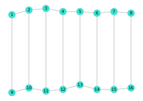
Figure 4: The graph of LD: The instance LD has 16 vertices and 22 edges. We are changing the edge demand along each edge to get LD_1, LD_2, and LD_3 in Table 3.

Table 3 shows the results for the first class of large demands instances (The detailed results are provided in Table 7 at Appendix 9 ). The column “sum(D)” gives the total spraying demand for each instance. The column “B_r” is the number of required robots of the basic robotic spraying formulation. The column “L_r” shows the number of multi-robotics (robots spraying multiple edges, mentioned in Definition 1) in the large edge demands formulation. “B_obj” and “L_obj” report the objective solution found by the basic and large edge demands model. The “B_gap” and “L_gap” are radio percentages with respect to the upper and lower bound of the basic and large edge demands models. “B_t” and “L_t” give the computing time of the two models (running times in seconds).

6.1 Computational results for Large edge demands instances

LD_1, LD_2, and LD_3 are instances with different edge demands. There exist some edges with requirements greater than the robot’s capacity. From Theorem 1, we know the large edge demands model works well if there have singleton robotic sprayers. Table 3 reports the computational results of the basic and large edge demands model with respect to these instances. The algorithms are implemented with 8 threads per CPU task. The Gurobi parameter random number “seed” acts as a small perturbation to the solver, and typically leads to different solution paths. We set the seed parameter to the values 1, 2, and 3. We displayed the average results from the three rounds.

Table 3 shows the large edge demands model outperforms the basic model regarding solution quality and has a faster computational time. A lower computational time for the large edge demands model indicates that there has fewer robot routes to optimize, which reduces the total number of variables. Besides, the basic model returns a big gap, whereas the large edge demands model reports a relatively small gap in all three instances. It is worth noting that parameter “seed” numbers lead to different solution paths, which may affect the average calculation. More specifically, the large edge demands reaches an optimal solution before 7200 seconds in some seed numbers, but some seed paths can not find the optimal solution in 7200 seconds. Thus the time is less than 7200 seconds and returns a small gap for the large edge demands model in Table 3.

Figures 5, 6 and 7 show the large demand instances’ performances in the branch-and-bound tree. The $x$ axis is time (s), and the $y$ axis is the value of the lower and upper bounds. The black solid line goes to the basic model, while the red dash-dotted lines represent the large edge demands model. The upper black solid and red dash-dotted lines show the changes in the upper bound of the basic and large edge demands model, respectively. Similarly, the bottom black and red dash-dotted lines reflect the changing of lower bounds. We use a consistent random number seed = 1.

Figure 5: LD_1 comparison results: The black solid and red dash-dotted lines are the upper and lower bounds of the basic and large edge demands model, respectively. We set seed =1, time limit =7200 seconds. The graph shows that the large edge demands model (red dash-dotted lines) has a fast convergence speed and returns a small gap.

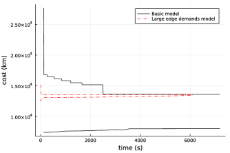
Figure 6: LD_2 comparison results: The black solid and red dash-dotted lines are the upper and lower bounds of the basic and large edge demands model, respectively. The graph shows that the large edge demands model (red dash-dotted lines) converges quickly and reaches optimal at about 6000 seconds, while the basic model still returns a big gap.

Figure 7: LD_3 comparison results: The black solid and red dash-dotted lines are the upper and lower bounds of the basic and large edge demands model, respectively. The graph shows that the large edge demands model (red dash-dotted lines) has a better root solution, whereas the basic model has a significant gap in the root node. The large edge demands model finds an optimal solution at about 4500 seconds, while the basic model returns a big gap.

6.2 Computational results for different techniques

The algorithms in Table 4 are described in Section 3 and Section 5. The first model is the basic model, denoted as the “Basic-model”. We add the lazy constraints to the basic model to get the result of “Lazy-constraints”. The symmetry elimination constraints continue to be added to obtain the result of “Sym-elimination”. Finally, we add the heuristic repair method to get the result of the“Heuristic-repair”. Besides, we check the performance of symmetry eliminations by getting rid of symmetry constraints from the heuristic repair method (“Heuristic-noSym”). The experiments are implemented with 32 threads per CPU task. We display the average data from the three rounds of different “seed” numbers. Different seed numbers generally lead to different solution paths and return similar solutions. However, it sometimes returns significant differences in time and solutions, remarkably affecting average values. The “obj” returns the objective solution. At the same time, the column “gap” is the deviation between the upper and lower bound. The column “t” displays the computing time in seconds, and the parameter “$\lvert Acc\rvert$” represents the number of accepted heuristic repair solutions.

Table 4 shows that the basic model only works for small-scale problems A and B. In contrast, lazy constraints and symmetry eliminations could solve medium-sized problems E and F. The heuristic repair method shows excellent solution quality and can be applied to large instances G. Computational time indicate that the Basic model is the most expensive one. At the same time, the other algorithms look similar to time consumption. We tested all of the algorithms in 7200 seconds (2 hours). After running 20 hours of instance G, we get a similar solution to the 2 hours solution, which shows the longer running time doesn’t improve the solution a lot.

Table 4: Comparative results of different techniques on the seven undirected instances from $A$ to $G$. This set was designed based on the real-world orchard data (Plessen et al.,, 2019). The column “sum(D)” is the total edge demands for the corresponding instance. Columns “obj” and “gap” show the optimal cost and deviation ($gap(\%)=100(UB-LB)/LB$, where $UB$ is the solution cost, and $LB$ is the lower bound ). The column “$\lvert Acc\rvert$” indicates the number of accepted heuristic solutions. The best performances are highlighted in grey cells, whereas the bold are the worst solution for each instance. Table 8 in Appendix 9 provides detailed results.

Ins. $\lvert N\rvert$ $\lvert E\rvert$ p r sum(D) Basic-model Lazy-constraints Sym-elimination Heuristic-repair Heuristic-noSym obj gap t (s) obj gap t (s) obj gap t (s) obj gap t (s) $\lvert Acc\rvert$ obj gap t (s) $\lvert Acc\rvert$ Ins.A 16 22 20 1 13.01 32.12 0.00% 0.85 32.12 0.00% 2.11 32.12 0.00% 1.98 32.12 0.00% 5.69 1 32.12 0.00% 4.26 1 Ins.B 20 28 20 1 17.14 42.64 0.00% 28.01 42.64 0.00% 2.07 42.64 0.00% 2.04 42.64 0.00% 5.97 1 42.64 0.00% 4.03 1 Ins.C 30 43 20 2 28.36 fail 76.15 0.00% 49.99 76.15 0.00% 62.07 76.15 0.00% 79.04 3 76.15 0.00% 91.90 3 Ins.D 42 61 20 2 32.58 fail 84.30 0.00% 5.74 84.30 0.00% 5.62 84.30 0.00% 10.93 6 84.30 0.00% 9.23 7 Ins.E 56 82 20 3 46.59 fail 127.65 2.68% 7200 127.65 3.62% 7200 127.65 2.45% 7200 8 127.65 2.75% 7200 6 Ins.F 78 115 20 3 52.98 fail 150.74 6.91% 7200 151.98 7.42% 7200 152.19 7.64% 7200 8 149.79 6.06% 7200 8 Ins.G 98 145 20 4 74.78 fail fail fail 235.77 15.75% 7200 13 251.58 20.72% 7200 6

The results of small-scale instances A and B show that all the algorithms could find an optimal solution, but it is considerably costlier for the heuristic repair method. This is because the heuristic repair method spends much time generating feasible solutions. As the size of the instances increases, the basic model fails to find an optimal solution in instances C and D, while other techniques work well. Instances E, F, and G show that the heuristic repair method works better in large-scale problems. Except for the heuristic technique, all the other methods failed to get solutions for the large-scale instance G. Table 4 shows that symmetry eliminations do not always work well in our instances. It saves time in test C and improves the solution quality for test E and G, but not helpful for the others. Our future work is to make symmetry eliminations work stable for our algorithms. As mentioned in Section 5, the heuristic repair method involves the parameter $\Gamma$, which affects the method’s overall performance. We reported in Section 4. We set $\Gamma$ = 1000 in this set of tests. Table 8 in Appendix 9 provides detailed results.

6.3 Computational results for benchmark instances

Table 5: Comparative results of the heuristic repair method with state-of-art algorithms from  Chen et al., (2016) on the 34 undirected instances of val set. This set was first designed to find CARP’s lower bound by Benavent et al., (1992). The column “Best-Known” is the best solution from previous literature. “LB” and “LB-H” show the lower bounds from the literature and this paper’s heuristic repair method, respectively. The better solutions are highlighted in grey cells, whereas the star indicates the solution matches the “Best-Known” solution.

File $\lvert N\rvert$ $\lvert E\rvert$ r p sum(D) LB LB-H Best-Known Heuristic-repair val1a 24 39 2 200 358 173 173 173 173* val1b 24 39 3 120 358 173 173 173 173* val1c 24 39 8 45 358 235 191 245 237 val2a 24 34 2 180 310 227 227 227 227* val2b 24 34 3 120 310 259 259 259 259* val2c 24 34 8 40 310 455 417 457 455 val3a 24 35 2 80 137 81 81 81 81* val3b 24 35 3 50 137 87 87 87 87* val3c 24 35 7 20 137 137 115 138 138* val4a 41 69 3 225 627 400 400 400 400* val4b 41 69 4 170 627 412 382 412 418 val4c 41 69 5 130 627 428 382 428 434 val4d 41 69 9 75 627 520 437 528 536 val5a 34 65 3 220 614 423 414 423 423* val5b 34 65 4 165 614 446 428 446 446* val5c 34 65 5 130 614 469 433 474 474* val5d 34 65 9 75 614 571 499 575 579 val6a 31 50 3 170 451 223 223 223 223* val6b 31 50 4 120 451 231 222 233 233* val6c 31 50 10 50 451 311 239 317 317* val7a 40 66 3 200 559 279 279 279 279* val7b 40 66 4 150 559 283 283 283 283* val7c 40 66 9 65 559 333 272 334 334* val8a 30 63 3 200 566 386 386 386 386* val8b 30 63 4 150 566 395 395 395 395* val8c 30 63 9 65 566 517 439 521 527 val9a 50 92 3 235 654 323 320 323 323* val9b 50 92 4 175 654 326 322 326 327 val9c 50 92 5 140 654 332 289 332 357 val9d 50 92 10 70 654 382 327 389 578 val10a 50 97 3 250 704 428 425 428 428* val10b 50 97 4 190 704 436 432 436 436* val10c 50 97 5 150 704 446 428 446 527 val10d 50 97 10 75 704 524 459 525 649

The set (val benchmark data set) contains 34 undirected instances designed by Benavent et al., (1992) to find the lower bounds of the CARP. These instances have been generated by varying the capacity of the vehicles for each graph (denoted val1a,valb,…,val10d). Table 5 reports the results for val benchmark data set. The columns “$\lvert N\rvert$” and “$\lvert E\rvert$” are the number of vertices and edges. The “r” is the number of vehicles, and “p” is the capacity of the identity vehicles. The “LB” is the lower bound are obtained by Belenguer et al., (2003). The column “Best-Known” are the best results reported in previous CARP literature (summarized by Chen et al., (2016)). Chen et al., (2016) presented a hybrid metaheuristic approach to solve the CARP. It is worth noting that all the results from other literature are not allowed to spit the demand along each required edge. The columns “LB-H” and “Heuristic-repair” are lower bounds and objective solutions computed by the heuristic repair method. The experiments are implemented with 32 threads per CPU task, seed = 1, $\Gamma$ = 4000.

Table 5 show that the heuristic repair method finds a better solution in instances “val1c” and “val2c” since our problem allows splitting the demand on a single demand edge amongst robots. Some latest works with these benchmark sets did not provide a detailed solution or generated new data sets based on Benavent et al., (1992) benchmark sets for an extension CARP. Arakaki et al., (2019) presented an efficiency-based path-scanning heuristic for the CARP, which introduced the concept of the efficiency rule. Arakki and Usberti’s results outperformed the other algorithms in average time but return a worse deviation (the average deviation comes from the lower bounds $GAP(\%)=100(UB-LB)/LB$, where $UB$ is the solution cost, and $LB$ is the lower bound) of val instances set. This paper focuses on the comparison of optimal cost results for val set. Thus, we make a comparison with Chen et al., (2016). We set the time limit to 2 hours and got an improved solution in val4B from 418 to 412 after extending the time limit to 3 hours. However, after increasing the time limit to 3 hours, the lower bound of most instances is slightly raised and returns the same objective solutions as 2 hours.

7 Parameter analysis of the heuristic repair method

The parameter $\Gamma$ represents the number of times the heuristic will be run without improvement before abandoning any further attempts to run the repair heuristic. As mentioned in Section 5, the parameter $\Gamma$ affects the heuristic repair method’s overall performance. This section analyzes the results related to the parameter $\Gamma$.

Fig. 8 shows the number of accepted heuristic solutions during the branch-and-bound process of Ins.G. It indicates that our heuristic repair method generates 15 solutions that are better than the current solutions found by the solver, which decreases the upper bound quickly. However, Fig. 8 shows the heuristic repair method generates 12 acceptable solutions at $\Gamma<3000$, while the last three solutions need to set a large $\Gamma$ but return a slightly changed upper bound. Thus, the selection of $\Gamma$ is crucial to the heuristic repair method.

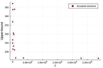
Figure 8: Accepted heuristic repair solutions of instance G: The x-axis is the number of $\Gamma$ whereas the y-axis is the current upper bound. The red dots represent the heuristic repair solutions. We set a relatively large initial number of $\Gamma=1\times 10^{6}$, and Gurobi accepted 15 heuristic repair solutions. However, the upper bound of the last three solutions decreased slightly with a large $\Gamma$. Further discussion about the selections of $\Gamma$ is worth studying.

Table 6 displays the “lower bound (LB)”, “upper bound (UB)”, and “gap” between LB and UB for different choices of heuristic repair parameter $\Gamma$ in the same graph instance G. The column “$\lvert Acc\rvert$” reports the number of accepted heuristic repair solutions. We use a consistent random number seed = 1.

Table 6: Ins.G: The column “LB” shows the lower bound of instance G, whereas “UB” presents the upper bound. The selections of $\Gamma$ between 1000 to 90000. The column “$\lvert Acc\rvert$” reports the number of accepted heuristic repair solutions, while the “gap” displays the deviation between the upper and lower bound.

$\Gamma$	LB	UB	gap	$\lvert Acc\rvert$
1000	199.0254	239.5126	16.90%	11
2000	198.7669	236.5206	15.96%	12
3000	198.8007	236.5206	15.95%	12
4000	198.7792	236.5155	15.96%	13
5000	198.7792	236.5155	15.96%	13
6000	198.6752	236.5155	16.00%	13
7000	198.7792	236.5155	15.96%	13
10000	198.6752	236.5155	16.00%	13
30000	198.4794	236.3278	16.02%	15
50000	198.4794	236.3278	16.02%	15
70000	198.4794	236.3278	16.02%	15
90000	198.4794	236.3278	16.02%	15

Table 6 shows that the best solution is $15.95\%$ at $\Gamma=3000$ with 12 acceptable heuristic repair solutions. Fig. 8 indicates the first 12 acceptable solutions decrease the upper bound significantly, while only slightly decreasing in the last three solutions. The small number choice of $\Gamma=1000$ generates 11 acceptable upper bounds, which does not generate a good upper bound for the branch-and-bound tree. Thus, it returns a bad solution of $16.90\%$. Besides, choosing a large number of $\Gamma$ is also expensive in generating unacceptable upper bounds, which are worst than the existing solutions. It is costly to set a large or small number of $\Gamma$, and a selection of 3000 to 4000 seems a reasonable first try for a large-scale problem.

8 Conclusions

In this paper, we proposed a splittable agricultural spraying vehicle routing problem. We are improving the formulation using theoretical insights about the optimal solution structure. This paper provides a SCARP model in two formulations: a basic spray and a large edge demand formulation. The large edge demands model outperforms the basic model in solving problems with high requirements for each edge. Solution methods consist of lazy constraints, symmetries elimination, and heuristic repair.

Tests on instances generated based on real data show the basic model is limited to small-scale problems, lazy constraints work well on medium-sized problems, and the heuristic repair method outperforms the other methods on large-scale trials. Moreover, the tested results indicated the SCARP model could provide cheaper solutions in some instances compared with the classical CARP.

The parameter test on $\Gamma$ analyzes parameter selections on the heuristic repair method, which makes the heuristic repair method work efficiently.

Further research can focus on selecting a more precise parameter $\Gamma$ for different problems to improve the efficiency of the heuristic repair method. Another direction is to study the accuracy of the solution to large-scale problems using meta-heuristic methods. The SCARP extension with nursing carts is also worth exploring in the next step.

Appendix A

9 Detailed data tables

Table 7: Details of computational results of Table 3. In addition to the data mentioned in Table 4, this table also provides the number of explored nodes in the column of “$\lvert ExploredNodes\rvert$”, and the number of simplex iterations in the branch-and-bound process in column “$\lvert SimplexIter\rvert$”.

Ins. Reports Basic_model Large_model LD_1 sum(D)=260.131 obj 6110.93 6110.93 LB 3845.45 6052.49 r 27 5 gap 37.07% 0.96% t 7200 7006.25 $\lvert ExploredNodes\rvert$ 3432 51575 $\lvert SimplexIter\rvert$ 553273 2516396 LD_2 sum(D)=390.195 obj 13675.18 13572.47 LB 8101.93 13503.11 r 40 5 gap 40.75% 0.51% t 7200 6358.96 $\lvert ExploredNodes\rvert$ 1 49770 $\lvert SimplexIter\rvert$ 56616 2715323 LD_3 sum(D)=520.26 obj 24058.06 23991.43 LB 14428.90 23832.65 r 53 4 gap 40.02 % 0.66% t 7200 6014.61 $\lvert ExploredNodes\rvert$ 79 44170 $\lvert SimplexIter\rvert$ 127326 2234217

Table 8: Details of computational results of Table 4. In addition to the data mentioned in Table 4, this table also provides the number of explored nodes in the column of “$\lvert ExploredNodes\rvert$”, and the number of simplex iterations in the branch-and-bound process in column “$\lvert SimplexIter\rvert$”.

Ins. Basic-model Lazy-constraints Symmetries elimination Heuristic repair H_no_sym Ins.A $\lvert N\rvert$= 16 $\lvert E\rvert$=22 p=20 r=1 sum(D)=13.0065 no obstacles obj 32.12 32.12 32.12 32.12 32.12 LB 32.12 32.12 32.12 32.12 32.12 gap 0.00% 0.00% 0.00% 0.00% 0.00% t(s) 0.85 2.11 1.98 5.69 4.26 $\lvert Acc\rvert$ – – – 1 1 $\lvert ExploredNodes\rvert$ 1 1 1 1 1 $\lvert SimplexIter\rvert$ 33 49 37 43 46 Ins.B $\lvert N\rvert$ =20 $\lvert E\rvert$=28 p=20 r=1 sum(D)=17.139 no obstacles obj 42.64 42.64 42.64 42.64 42.64 LB 42.64 42.64 42.64 42.64 42.64 gap 0.00% 0.00% 0.00% 0.00% 0.00% t(s) 28.01 2.07 2.04 5.97 4.03 $\lvert Acc\rvert$ – – – 1 1 $\lvert ExploredNodes\rvert$ 1 1 7 5 1 $\lvert SimplexIter\rvert$ 71 68 79 124 82 Ins.C $\lvert N\rvert$ =30 $\lvert E\rvert$=43 p=20 r=2 sum(D)=28.362 no obstacles obj fail 76.15 76.15 76.15 76.15 LB – 76.15 76.15 76.15 76.15 gap – 0.00% 0.00% 0.00% 0.00% t(s) – 49.99 62.07 79.04 91.90 $\lvert Acc\rvert$ – – – 3.33 3 $\lvert ExploredNodes\rvert$ – 317766 375578 420542 535452 $\lvert SimplexIter\rvert$ – 3977670 4971315 5590590 6569088 Ins.D $\lvert N\rvert$ =42 $\lvert E\rvert$=61 p=20 r=2 sum(D)=32.5815 with a obstacle obj fail 84.30 84.30 84.30 84.30 LB – 84.30 84.30 84.30 84.30 gap – 0.00% 0.00% 0.00% 0.00% t(s) – 5.74 5.62 10.93 9.23 $\lvert Acc\rvert$ – – – 6 7 $\lvert ExploredNodes\rvert$ – 5761 4424 7742 7656 $\lvert SimplexIter\rvert$ – 143823 109771 168798 178461 Ins.E $\lvert N\rvert$ =56 $\lvert E\rvert$=82 p=20 r=3 sum(D)=46.59 with a obstacle obj fail 127.65 127.65 127.65 127.65 LB – 124.23 123.03 124.52 124.14 gap – 2.68% 3.62% 2.45% 2.75% t(s) – 7200 7200 7200 7200 $\lvert Acc\rvert$ – – – 8 6 $\lvert ExploredNodes\rvert$ – 4509341 4298279 5212149 5145643 $\lvert SimplexIter\rvert$ – 371701414 349635575 447436137 426000722 Ins.F $\lvert N\rvert$ =78 $\lvert E\rvert$=115 p=20 r=3 sum(D)=52.983 with two obstacles obj fail 150.74 151.98 152.19 149.79 LB – 140.31 140.67 140.57 140.69 gap – 6.91% 7.42% 7.64% 6.06% t(s) – 7200 7200 7200 7200 $\lvert Acc\rvert$ – – – 8 8 $\lvert ExploredNodes\rvert$ – 322947 425121 444244 400689 $\lvert SimplexIter\rvert$ – 47437951 63547502 61216769 63985627 Ins.G $\lvert N\rvert$ =98 $\lvert E\rvert$=145 p=20 r=4 sum(D)=74.7765 with two obstacles obj fail fail fail 235.77 251.58 LB – – – 198.60 199.21 gap – – – 15.75% 20.72% t(s) – – – 7200 7200 $\lvert Acc\rvert$ – – – 13 6 $\lvert ExploredNodes\rvert$ – – – 177727 175286 $\lvert SimplexIter\rvert$ – – – 20497276 17737926

References

- Amponsah et al., (2004) Amponsah, Samuel Kwame and Salhi, Said, 2004. The Investigation of a Class of Capacitated Arc Routing Problems: The Collection of Garbage in Developing Countries, Waste Management, 24, 7, 711–721.
- Arakaki et al., (2019) Arakaki, Rafael Kendy and Usberti, Fabio Luiz, 2019. An efficiency-based path-scanning heuristic for the capacitated arc routing problem, Computers & Operations Research, 103, 288–295.
- Archetti et al., (2012) Archetti, Claudia and Speranza, Maria Grazia, 2012. Vehicle routing problems with split deliveries, International transactions in operational research, 19, 1-2, 3–22.
- Baldacci et al., (2006) Baldacci, Roberto and Maniezzo, Vittorio, 2006. Exact methods based on node-routing formulations for undirected arc-routing problems, Networks, 47, 1, 52–60.
- Barth et al., (2016) Barth, Ruud and Hemming, Jochen and van Henten, Eldert J, 2016. Design of an eye-in-hand sensing and servo control framework for harvesting robotics in dense vegetation, Biosystems Engineering, 146, 71–84.
- Belenguer et al., (2003) Belenguer, José M and Benavent, Enrique, 2003. A cutting plane algorithm for the capacitated arc routing problem, Computers & Operations Research, 30, 5, 705–728.
- Belenguer et al., (2015) Belenguer, José Manuel and Benavent, Enrique and Irnich, Stefan, 2015. Chapter 9: The capacitated arc routing problem: Exact algorithms. In Arc routing: problems, methods, and applications, SIAM, 183–221.
- Benavent et al., (1992) Benavent, Enrique and Campos, Vicente and Corberán, Angel and Mota, Enrique, 1992. The Capacitated Arc Routing Problem: Lower Bounds, Networks, 22, 7, 669–690.
- Braekers et al., (2016) Braekers, Kris and Ramaekers, Katrien and Van Nieuwenhuyse, Inneke, 2016. The vehicle routing problem: State of the art classification and review, Computers & Industrial Engineering, 99, 300–313.
- Campbell et al., (2000) Campbell, James F and Langevin, Andre, 2000. Roadway snow and ice control, In Arc Routing. Springer, pp. 389–418.
- Cay et al., (2018) Cay, Anil and Kocabiyik, Habib and May, Sahin, 2018. Development of an electro-mechanic control system for seed-metering unit of single seed corn planters part i: Design and laboratory simulation, Computers and Electronics in Agriculture, 71–79.
- Chen et al., (2016) Chen, Yuning and Hao, Jin-Kao and Glover, Fred, 2016. A hybrid metaheuristic approach for the capacitated arc routing problem, European Journal of Operational Research, 253, 1, 25–39.
- Chiang et al., (2014) Chiang, Tsung-Che and Hsu, Wei-Huai, 2014. A knowledge-based evolutionary algorithm for the multiobjective vehicle routing problem with time windows, Computers & Operations Research, 45, 25–37.
- Dantzig et al., (1959) Dantzig, George B and Ramser, John H, 1959. The truck dispatching problem, Management Science, 6, 1, 80–91.
- Dror et al., (2012) Dror, Moshe, 2012. Arc routing: theory, solutions and applications, Springer Science & Business Media.
- Eglese et al., (1994) Eglese, Richard W, 1994. Routeing winter gritting vehicles, Discrete Applied Mathematics, 48, 3, 231–244.
- Eiselt et al., 1995 (a) Eiselt, Horst A and Gendreau, Michel and Laporte, Gilbert, 1995. Arc routing problems, part i: The chinese postman problem, Operations Research, 43, 2, 231–242.
- Eiselt et al., 1995 (b) Eiselt, Horst A and Gendreau, Michel and Laporte, Gilbert, 1995. Arc routing problems, part ii: The rural postman problem, Operations Research, 43, 3, 399–414.
- Golden et al., (1981) Golden, Bruce L and Wong, Richard T, 1981. Capacitated arc routing problems, Networks, 11, 3, 305–315.
- Grötschel et al., (1985) Grötschel, Martin and Padberg, Manfred W and others, 1985. Polyhedral theory, The traveling salesman problem, 251–305.
- Hertz et al., (2000) Hertz, Alain and Laporte, Gilbert and Mittaz, Michel, 2000. A tabu search heuristic for the capacitated arc routing problem, Operations Research, 48, 1, 129–135.
- Keskin et al., (2019) Keskin, Muhammed Emre and Yılmaz, Mustafa, 2019. Chinese and windy postman problem with variable service costs, Soft Computing, 23, 16, 7359–7373.
- Khazimov et al., (2018) Khazimov, Z.M., Bora, G., Khazimov, K., Khazimov, M., Ultanova, I., Niyazbayev, A., 2018. Development of a dual action planting and mulching machine for vegetable seedlings, Engineering in Agriculture, Environment and Food, 11, 2, 74–78.
- Lacomme et al., (2004) Lacomme, Philippe and Prins, Christian and Ramdane-Cherif, Wahiba. Competitive memetic algorithms for arc routing problems, 2004, Annals of Operations Research, 131, 1, 159–185.
- Laporte et al., (1992) Laporte, Gilbert, 1992. The vehicle routing problem: An overview of exact and approximate algorithms, European Journal of Operational Research, 59, 3, 345–358.
- Lenstra et al., (1976) Lenstra, Jan Karel and Kan, AHG Rinnooy, 1976. On general routing problems, Networks, 6, 3, 273–280.
- Lenstra et al., (1981) Lenstra, Jan Karel and Kan, AHG Rinnooy, 1981. Complexity of vehicle routing and scheduling problems, Networks, 221–227.
- Lysgaard et al., (2020) Lysgaard, Jens and López-Sánchez, Ana Dolores and Hernández-Díaz, Alfredo G, 2020. A matheuristic for the minmax capacitated open vehicle routing problem, International Transactions in Operational Research, 27, 1, 394–417.
- Mahajan et al., (2015) Mahajan, Shveta and Das, Amitava and Sardana, Harish Kumar, 2015. Image acquisition techniques for assessment of legume quality, Trends in Food Science & Technology, 42, 2, 116–133.
- Mahmud et al., (2020) Mahmud, M.S.A., Abidin, M.S.Z., Emmanuel, A.A., and Hasan, H.S., 2020. Robotics and automation in agriculture: present and future applications, Applications of Modelling and Simulation, 4, 130–140.
- Monroy-Licht et al., (2017) Monroy-Licht, Marcela and Amaya, Ciro Alberto and Langevin, André and Rousseau, Louis-Martin, 2017. The rescheduling arc routing problem, International Transactions in Operational Research, 24, 6, 1325–1346.
- Muthukumaran et al., (2021) Muthukumaran, S and Ganesan, Manikandan and Dhanasekar, J and Babu Loganathan, Ganesh, 2021. Path planning optimization for agricultural spraying robots using hybrid dragonfly–cuckoo search algorithm, Alinteri Journal of Agriculture Sciences, 36, 1, 2564–7814.
- Oberti er al., (2016) Oberti, Roberto and Marchi, Massimo and Tirelli, Paolo and Calcante, Aldo and Iriti, Marcello and Tona, Emanuele and Hočevar, Marko and Baur, Joerg and Pfaff, Julian and Schütz, Christoph and others, 2016. Selective spraying of grapevines for disease control using a modular agricultural robot, Biosystems Engineering, 146, 203–215.
- Ozguven et al., (2019) Ozguven, Mehmet Metin and Adem, Kemal, 2019. Automatic detection and classification of leaf spot disease in sugar beet using deep learning algorithms, Physica A: Statistical Mechanics and Its Applications, 535, 122537.
- Plessen et al., (2019) Plessen, Mogens Graf, 2019. Optimal in-field routing for full and partial field coverage with arbitrary non-convex fields and multiple obstacle areas, Biosystems Engineering, 186, 234–245.
- Quintero-Araujo et al., (2017) Quintero-Araujo, C.L., Caballero-Villalobos, J.P., Juan, A.A, Montoya-Torres, J.R., 2017. A biased-randomized metaheuristic for the capacitated location routing problem, International Transactions in Operational Research, 24, 5, 1079–1098.
- Santos et al., (2010) Santos, Luís and Coutinho-Rodrigues, João and Current, John R, 2010. An improved ant colony optimization based algorithm for the capacitated arc routing problem, Transportation Research Part B: Methodological, 44, 2, 246–266.
- Shi et al., (2019) Shi, Y., Rex, S.X., Wang, X., Hu, Z., Newman, D., Ding, W., 2019. Numerical simulation and field tests of minimum-tillage planter with straw smashing and strip laying based on edem software, Computers and Electronics in Agriculture, 105021.
- Singh et al., (2017) Singh, Vijai and Misra, Ak K, 2017. Detection of plant leaf diseases using image segmentation and soft computing techniques, Information Processing in Agriculture, 4, 1, 41–49.
- Gonzalez-de-Soto et al., (2016) Gonzalez-de-Soto, Mariano and Emmi, Luis and Perez-Ruiz, Manuel and Aguera, Juan and Gonzalez-de-Santos, Pablo, 2016. Autonomous systems for precise spraying–evaluation of a robotised patch sprayer, Biosystems Engineering, 165–182.
- Toth et al., (2014) Toth, Paolo and Vigo, Daniele, 2014. Vehicle routing: problems, methods, and applications, SIAM.
- Vakilian et al., (2017) Vakilian, Keyvan Asefpour and Massah, Jafar, 2017. A farmer-assistant robot for nitrogen fertilizing management of greenhouse crops, Computers and Electronics in Agriculture, 139, 153–163.
- Williams et al., (2019) Williams, Henry AM and Jones, Mark H and Nejati, Mahla and Seabright, Matthew J and Bell, Jamie and Penhall, Nicky D and Barnett, Josh J and Duke, Mike D and Scarfe, Alistair J and Ahn, Ho Seok and others, 2019. Robotic kiwifruit harvesting using machine vision, convolutional neural networks, and robotic arms, Biosystems Engineering, 181, 140–156.
- Xiong et al., (2019) Xiong, Ya and Peng, Cheng and Grimstad, Lars and From, Pål Johan and Isler, Volkan, 2019. Development and field evaluation of a strawberry harvesting robot with a cable-driven gripper, Computers and Electronics in Agriculture, 157, 392–402.
- Xu et al., (2022) Xu, Jiahong and Lai, Jing and Guo, Rui and Lu, Xiaoxiao and Xu, Lihong, 2022. Efficiency-oriented mpc algorithm for path tracking in autonomous agricultural machinery, Agronomy, 12, 7, 1662.