Octant Degeneracy and Plots of Parameter Degeneracy in Neutrino Oscillations Revisited

Sho Sugama and Osamu Yasuda

Abstract

The three kinds of parameter degeneracy in neutrino oscillation, the intrinsic, sign and octant degeneracy, form an eight-fold degeneracy. The nature of this eight-fold degeneracy can be visualized on the ($\sin^{2}2\theta_{13}$, $1/\sin^{2}\theta_{23}$)-plane, through quadratic curves defined by $P(\nu_{\mu}\to\nu_{e})=$ const. and $P(\bar{\nu}_{\mu}\to\bar{\nu}_{e})=$ const., along with a straight line $P(\nu_{\mu}\to\nu_{\mu})=$ const. After $\theta_{13}$ was determined by reactor neutrino experiments, the intrinsic degeneracy in $\theta_{13}$ transforms into an alternative octant degeneracy in $\theta_{23}$, which can potentially be resolved by incorporating the value of $P(\nu_{\mu}\to\nu_{\mu})$. In this paper, we analytically discuss whether this octant parameter degeneracy is resolved or persists in the future long baseline accelerator neutrino experiments, such as T2HK, DUNE, T2HKK and ESS$\nu$SB. It is found that the energy spectra near the first oscillation maximum are effective in resolving the octant degeneracy, whereas those near the second oscillation maximum are not.

1 Introduction

In the past twenty-five years, significant progress have been achieved in measuring neutrino oscillation parameters within the standard three-flavor framework [1]. The ultimate goal in the study of standard neutrino oscillations is to determine the CP phase $\delta$. It is expected that future long baseline experiments such as T2HK [2] and DUNE [3] will precisely measure the appearance probabilities $P(\nu_{\mu}\to\nu_{e})$ and $P(\bar{\nu}_{\mu}\to\bar{\nu}_{e})$, enabling the determination of $\delta$. However, an issue arises in extracting $\delta$ from appearance probabilities due to the so-called parameter degeneracy. This implies that even with precise knowledge of $P(\nu_{\mu}\to\nu_{e})$ and $P(\bar{\nu}_{\mu}\to\bar{\nu}_{e})$ at a fixed energy and baseline length, these probabilities cannot uniquely determine the values of ($\theta_{23}$, $\theta_{13}$, $\delta$). Since each degenerate solution gives a different value of $\delta$, resolving the parameter degeneracy is crucial for the precise determination of $\delta$. In historical context, the octant degeneracy $\pi/4-\theta_{23}\leftrightarrow\theta_{23}-\pi/4$ was first identified in Ref. [4], followed by the recognition of the intrinsic degeneracy in Ref. [5], and the sign degeneracy $\Delta m^{2}_{\mbox{\rm\scriptsize atm}}\leftrightarrow-\Delta m^{2}_{\mbox{\rm\scriptsize atm}}$ in Ref. [6]. Ref. [7] highlighted the presence of these as eight-fold degeneracies. Moreover, a graphical representation was introduced in Ref. [8] where curves derived from $P(\nu_{\mu}\rightarrow\nu_{e})=$ const. and $P(\bar{\nu}_{\mu}\rightarrow\bar{\nu}_{e})=$ const. formed quadratic patterns on the ($X\equiv\sin^{2}2\theta_{13}$, $Y\equiv 1/s^{2}_{23}$)-plane, where $s_{23}\equiv\sin\theta_{23}$. The representation in Ref. [8] visually demonstrates the existence of eight degenerate solutions, as elaborated in the subsequent section.

After the determination of $\theta_{13}$ through reactor experiments  [9, 10, 11], the primary focus shifts to the sign degeneracy of $\Delta m^{2}_{\mbox{\rm\scriptsize atm}}$ and the octant degeneracy of $\theta_{23}$. As far as the sign degeneracy is concerned, nearly all results favor the normal ordering (NO) over the inverted ordering (IO) [1]. As for the octant degeneracy, on the other hand, uncertainty remains regarding the correct octant, as the Superkamiokande atmospheric neutrino results seem to favor the lower octant, while other datasets indicate a different preference [12].

The purpose of this work is to investigate the behavior of the octant degeneracy when combining appearance probabilities $P(\nu_{\mu}\rightarrow\nu_{e})=$ const. and $P(\bar{\nu}_{\mu}\rightarrow\bar{\nu}_{e})=$ const. with fixed values of $X\equiv\sin^{2}2\theta_{13}=$ const. and $Y\equiv 1/s^{2}_{23}=$ const., utilizing the graphical representation from Ref. [8] for the T2HK [2], T2HKK [13], DUNE [3], and ESS$\nu$SB [14] experiments. Our results demonstrate that, by utilizing energy bins near the first oscillation maximum, the octant degeneracy can be resolved by ensuring the intersection of these quadratic curves with the vertical line $X=$ const. and the two horizontal lines ($Y=2/(1\pm\sqrt{1-\sin^{2}2\theta_{23}})$), under the assumption of small experimental errors.

The paper is organized as follows. In Sect. 2, we provide background information on parameter degeneracy and introduce the plot illustrating the eight-fold parameter degeneracy. Sect. 3 presents the plots for the four future long baseline experiments and discusses the distinctive characteristics of each experiment. Finally, Section 4 summarizes our conclusions.

2 The plot of the eight-fold parameter degeneracy

In the second-order approximation with respect to $\theta_{13}$ and $\Delta m_{21}^{2}$, the appearance probabilities $P(\nu_{\mu}\to\nu_{e},E)$ and $P(\bar{\nu}_{\mu}\to\bar{\nu}_{e},E)$ for a neutrino energy $E$ and a baseline length $L$ can be expressed as [15, 7]

$$P(\nu_{\mu}\to\nu_{e},E)=x^{2}F^{2}+2\,\mbox{\rm sign}(\Delta m_{31}^{2})\,xyFg\cos\left[\delta+\mbox{\rm sign}(\Delta m_{31}^{2})\,\Delta\right]+y^{2}g^{2}$$ (1)

$$P(\bar{\nu}_{\mu}\to\bar{\nu}_{e},E)=x^{2}\bar{F}^{2}+2\,\mbox{\rm sign}(\Delta m_{31}^{2})\,xy\bar{F}g\cos\left[\delta-\mbox{\rm sign}(\Delta m_{31}^{2})\,\Delta\right]+y^{2}g^{2}\,,$$ (2)

where

$$x\equiv s_{23}\sin 2\theta_{13}\,,$$ (5)

$$y\equiv\left|\frac{\Delta m^{2}_{21}}{\Delta m^{2}_{31}}\right|\cos\theta_{23}\sin 2\theta_{12}\,,$$

$$(F,\bar{F})\equiv\left\{\begin{array}[]{c}(f,\bar{f})~{}~{}\mbox{\rm for NO}\\ (\bar{f},f)~{}~{}\mbox{\rm for IO}\\ \end{array}\right\}\,,$$

$$\left\{\begin{array}[]{c}f\\ \bar{f}\end{array}\right\}\equiv\frac{\sin\left(\Delta\mp AL/2\right)}{\left(1\mp AL/2\Delta\right)}\,,$$ (8)

$$g\equiv\frac{\sin\left(AL/2\right)}{AL/2\Delta}\,,$$

$$\Delta\equiv\frac{|\Delta m_{31}^{2}|L}{4E}\,,$$

$$A\equiv\sqrt{2}G_{F}N_{e}\,,$$

$G_{F}$ stands for the Fermi coupling constant, and $N_{e}$ represents the electron density in matter, which we assume to be constant throughout this paper.

In the experiment, based on the measured values of the oscillation probabilities

$$P(E)\equiv P(\nu_{\mu}\to\nu_{e},E;\theta_{jk}^{\,\scriptsize{\mbox{\rm true}}},\Delta m_{jk}^{2\ \scriptsize{\mbox{\rm true}}},\delta^{\,\scriptsize{\mbox{\rm true}}})$$ (9)

and

$$\bar{P}(E)\equiv P(\bar{\nu}_{\mu}\to\bar{\nu}_{e},E;\theta_{jk}^{\,\scriptsize{\mbox{\rm true}}},\Delta m_{jk}^{2\ \scriptsize{\mbox{\rm true}}},\delta^{\,\scriptsize{\mbox{\rm true}}})\,,$$ (10)

which are functions of the true oscillation parameters and remain fixed, we attempt to adjust the values of $P(\nu_{\mu}\to\nu_{e},E;\theta_{jk}^{\,\scriptsize{\mbox{\rm test}}},\Delta m_{jk}^{2\ \scriptsize{\mbox{\rm test}}},\delta^{\,\scriptsize{\mbox{\rm test}}})$ and $P(\bar{\nu}_{\mu}\to\bar{\nu}_{e},E;\theta_{jk}^{\,\scriptsize{\mbox{\rm test}}},\Delta m_{jk}^{2\ \scriptsize{\mbox{\rm test}}},\delta^{\,\scriptsize{\mbox{\rm test}}})$, which depend on the test oscillation parameters, to match $P(E)$ and $\bar{P}(E)$ by varying the test oscillation parameters. The present study focuses on the following question: Given the two appearance probabilities $P(E)$ and $\bar{P}(E)$ at a given energy $E$, can we uniquely determine the oscillation probabilities? In other words, do the two equations

$$P(\nu_{\mu}\to\nu_{e},E;\theta_{jk}^{\,\scriptsize{\mbox{\rm test}}},\Delta m_{jk}^{2\ \scriptsize{\mbox{\rm test}}},\delta^{\,\scriptsize{\mbox{\rm test}}})=P(\nu_{\mu}\to\nu_{e},E;\theta_{jk}^{\,\scriptsize{\mbox{\rm true}}},\Delta m_{jk}^{2\ \scriptsize{\mbox{\rm true}}},\delta^{\,\scriptsize{\mbox{\rm true}}})$$ (11)

$$P(\bar{\nu}_{\mu}\to\bar{\nu}_{e},E;\theta_{jk}^{\,\scriptsize{\mbox{\rm test}}},\Delta m_{jk}^{2\ \scriptsize{\mbox{\rm test}}},\delta^{\,\scriptsize{\mbox{\rm test}}})=P(\bar{\nu}_{\mu}\to\bar{\nu}_{e},E;\theta_{jk}^{\,\scriptsize{\mbox{\rm true}}},\Delta m_{jk}^{2\ \scriptsize{\mbox{\rm true}}},\delta^{\,\scriptsize{\mbox{\rm true}}})$$ (12)

give unique values of the test oscillation parameters, in particular of the test CP phase $\delta^{\,\scriptsize{\mbox{\rm test}}}$? We know that the answer to this question is negative because parameter degeneracy affects the CP phase $\delta^{\,\scriptsize{\mbox{\rm test}}}$, as well as the mixing angles $\theta_{13}^{\,\scriptsize{\mbox{\rm test}}}$ and $\theta_{23}^{\,\scriptsize{\mbox{\rm test}}}$, at a given neutrino energy $E$. We will keep the values of $\Delta m_{31}^{2\ \scriptsize{\mbox{\rm test}}}$, $\Delta m_{21}^{2\ \scriptsize{\mbox{\rm test}}}$ and $\theta_{12}^{\,\scriptsize{\mbox{\rm test}}}$ fixed, while varying $\delta^{\,\scriptsize{\mbox{\rm test}}}$, $\theta_{13}^{\,\scriptsize{\mbox{\rm test}}}$ and $\theta_{23}^{\,\scriptsize{\mbox{\rm test}}}$ as test variables around their true values. In the following discussions, we omit the superscript “test” of the test oscillation parameters for simplicity. In Eqs. (9) and (10), $P(E)$ and $\bar{P}(E)$ are the probabilities evaluated using the true oscillation parameters $\delta^{\,\scriptsize{\mbox{\rm true}}}$, $\theta_{13}^{\,\scriptsize{\mbox{\rm true}}}$ and $\theta_{23}^{\,\scriptsize{\mbox{\rm true}}}$ at the neutrino energy $E$, whereas $x^{2}F^{2}+2\,\mbox{\rm sign}(\Delta m_{31}^{2})\,xyFg\cos\left[\delta+\mbox{\rm sign}(\Delta m_{31}^{2})\,\Delta\right]+y^{2}g^{2}$ and $x^{2}\bar{F}^{2}+2\,\mbox{\rm sign}(\Delta m_{31}^{2})\,xy\bar{F}g\cos\left[\delta-\mbox{\rm sign}(\Delta m_{31}^{2})\,\Delta\right]+y^{2}g^{2}$ in Eqs. (1) and (2) are calculated with the test values of $\delta$, $\theta_{13}$ and $\theta_{23}$. By introducing the new variables

$$X\equiv\sin^{2}2\theta_{13}$$

$$Y\equiv\displaystyle\frac{1}{s^{2}_{23}}\,,$$

which are functions of the test oscillation parameters, expressing $\cos\delta$ and $\sin\delta$ from Eqs. (1) and (2) as

$$\cos\delta=\frac{1}{4\mbox{\rm sign}(\Delta m_{31}^{2})xyg\cos\Delta}\left(\frac{P(E)-x^{2}F^{2}-y^{2}g^{2}}{F}+\frac{\bar{P}(E)-x^{2}\bar{F}^{2}-y^{2}g^{2}}{\bar{F}}\right)$$ (13)

$$\sin\delta=\frac{1}{4\mbox{\rm sign}(\Delta m_{31}^{2})xyg\sin\Delta}\left(-\frac{P(E)-x^{2}F^{2}-y^{2}g^{2}}{F}+\frac{\bar{P}(E)-x^{2}\bar{F}^{2}-y^{2}g^{2}}{\bar{F}}\right),$$ (14)

and subsequently eliminating the test CP phase $\delta$, we obtain the following expression from Eqs. (11), (12),  (1) and (2) [8]:

$$16CX(Y-1)$$ (15)

$$=\frac{1}{\cos^{2}\Delta}\left[\left(\frac{P(E)-C}{F}+\frac{\bar{P}(E)-C}{\bar{F}}\right)(Y-1)-(F+\bar{F})X+\frac{P(E)}{F}+\frac{\bar{P}(E)}{\bar{F}}\right]^{2}$$

$$+\frac{1}{\sin^{2}\Delta}\left[\left(\frac{P(E)-C}{F}-\frac{\bar{P}(E)-C}{\bar{F}}\right)(Y-1)-(F-\bar{F})X+\frac{P(E)}{F}-\frac{\bar{P}(E)}{\bar{F}}\right]^{2},$$

where

$$C\equiv\left(\frac{\Delta m^{2}_{21}}{\Delta m^{2}_{31}}\right)^{2}\left[\frac{\sin(AL/2)}{AL/2\Delta}\right]^{2}\sin^{2}2\theta_{12}\,.$$

In energy ranges where $|\Delta m_{31}^{2}|L/4E\neq n\pi/2$ ($n=1,2,3,\cdots$) is satisfied, Eq. (15) represents a quadratic curve in the $(X,Y)$-plane [8]. Notice that $X$ and $Y$ are the test variables for fitting, whereas $P(E)$ and $\bar{P}(E)$ are fixed for a given energy $E$ because they depend on the true oscillation parameters and the neutrino energy $E$. Note also that a different point on the quadratic curve corresponds to a different value of the test CP phase $\delta$, because Eqs. (13) and (14) shows that $\delta$ can be uniquely defined by $x=\sqrt{X/Y}$ and $y=|\Delta m^{2}_{21}/\Delta m^{2}_{31}|\sin 2\theta_{12}\sqrt{1-1/Y}$. The rationale behind choosing the variable $Y\equiv 1/s^{2}_{23}$ is its analytical convenience for demonstrating that there exist two intersections between the curve (15) and the line $\theta_{23}=$ const. Depending on whether the test mass ordering is correct or wrong, i.e., whether the test mass ordering matches the true ordering or not, two potential quadratic curves emerge, as depicted in Fig. 1 (a). By utilizing the disappearance probability $P(\nu_{\mu}\to\nu_{\mu})\sim\sin^{2}2\theta_{23}\sin^{2}(\Delta m_{31}^{2}L/4E)$, we can infer the value of $\sin^{2}2\theta_{23}$, which yields two possibilities for

$$Y=\left\{\begin{array}[]{l}Y^{\scriptsize{\mbox{\rm HO}}}\\ Y^{\scriptsize{\mbox{\rm LO}}}\end{array}\right\}\equiv\frac{2}{1\pm\sqrt{1-\sin^{2}2\theta_{23}^{\,\scriptsize{\mbox{\rm true}}}}}\,,$$ (18)

where the superscript HO (LO) stands for high (low) octant. The ambiguity of choosing between $Y^{\scriptsize{\mbox{\rm HO}}}$ and $Y^{\scriptsize{\mbox{\rm LO}}}$ represents the octant degeneracy. Prior to the measurement of $\theta_{13}$, therefore, there were potentially eight solutions, as illustrated in Fig. 1 (a). Since a different point on the quadratic curves corresponds to a different value of the test CP phase $\delta$, Fig. 1 (a) implies that the eight-fold degeneracy in general gives eight different values for the test CP phase $\delta$.

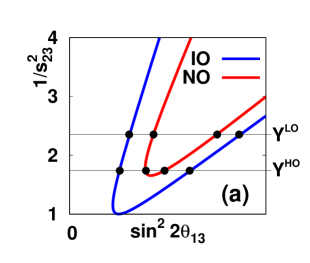
Figure 1: Parameter degeneracy for normal ordering and inverted ordering. $1/s_{23}^{2}=Y^{\scriptsize{\mbox{\rm LO}}}$ or $1/s_{23}^{2}=Y^{\scriptsize{\mbox{\rm HO}}}$, where $Y^{\scriptsize{\mbox{\rm LO}}}$ and $Y^{\scriptsize{\mbox{\rm HO}}}$ are given by Eq. (18), is obtained from the disappearance probability $P(\nu_{\mu}\to\nu_{\mu})$. (a) Away from the oscillation maximum ($|\Delta m^{2}_{31}|L/4E\neq\pi/2$), (b) At the oscillation maximum ($|\Delta m^{2}_{31}|L/4E=\pi/2$). In the case of (a), there are eight solutions with a different value of $\delta$. In the case of (b), four solutions exist with a two-fold degeneracy.

Conversely, at the oscillation maximum ($|\Delta m_{31}^{2}|L/4E=\left(n+1/2\right)\pi$; $n=0,1,2,\cdots$), the numerator of the first term on the right hand side of Eq. (15) must vanish, resulting in a straight line in the $(X,Y)$-plane:

$$\left(\frac{P(E)-C}{F}+\frac{\bar{P}(E)-C}{\bar{F}}\right)(Y-1)-(F+\bar{F})X+\frac{P(E)}{F}+\frac{\bar{P}(E)}{\bar{F}}=0\,.$$ (19)

In this case, two potential straight lines also emerge, and they are illustrated in Fig. 1 (b). When considering the situation at the oscillation maximum, there exist four feasible solutions, each characterized by a two-fold degeneracy, as the two-fold intrinsic degeneracy is exact in this case.

Given our primary focus on the intersection between curve (15) and $\sin^{2}2\theta_{13}=$ const. or $1/s^{2}_{23}=$ const., the classification of the quadratic curve (15) as hyperbolic or elliptic does not directly influence the parameter degeneracy characteristics. However, it is feasible to ascertain whether curve (15) is hyperbolic or elliptic based on the sign of the following discriminant:

$$D\equiv\left[\frac{1}{\cos^{2}\Delta}\left(\frac{P(E)-C}{F}+\frac{\bar{P}(E)-C}{\bar{F}}\right)(F+\bar{F})\right.$$ (20)

$$+\left.\frac{1}{\sin^{2}\Delta}\left(\frac{P(E)-C}{F}-\frac{\bar{P}(E)-C}{\bar{F}}\right)(F-\bar{F})+8C\right]^{2}$$

$$-\left[\frac{1}{\cos^{2}\Delta}\left(\frac{P(E)-C}{F}+\frac{\bar{P}(E)-C}{\bar{F}}\right)^{2}+\frac{1}{\sin^{2}\Delta}\left(\frac{P(E)-C}{F}-\frac{\bar{P}(E)-C}{\bar{F}}\right)^{2}\right]$$

$$\times\left[\frac{1}{\cos^{2}\Delta}(F+\bar{F})^{2}+\frac{1}{\sin^{2}\Delta}(F-\bar{F})^{2}\right]\,,$$

where $D>0$ ($D<0$) corresponds to a hyperbolic (an elliptic) curve. In general, in the energy region near the first oscillation maximum ($|\Delta m_{31}^{2}|L/4E\sim\pi/2$), curve (15) exhibits a hyperbolic shape, whereas it can have an elliptic form in the lower energy region, as explained in the subsequent discussions for each future experiment.

3 Behaviors of the plots for the future long baseline experiments

After $\theta_{13}$ was determined, the situation of the eight-fold parameter degeneracy is changed. The following three pieces of information are available:

(i)The quadratic curve derived from

$$P(\nu_{\mu}\to\nu_{e})=\mbox{\rm const}.~{}\&~{}P(\bar{\nu}_{\mu}\to\bar{\nu}_{e})=\mbox{\rm const}.$$

$$\mbox{\rm(ii)}~{}\mbox{\rm The~{}straight~{}line~{}}X=\mbox{\rm const}.\mbox{\rm~{}obtained~{}from}$$

$$P(\bar{\nu}_{e}\to\bar{\nu}_{e})=\mbox{\rm const}.$$

$$\mbox{\rm(iii)}~{}\mbox{\rm The~{}straight~{}line~{}}Y=\mbox{\rm const}.\mbox{\rm~{}obtained~{}from}$$

$$P(\nu_{\mu}\to\nu_{\mu})=\mbox{\rm const}.~{}\&~{}P(\bar{\nu}_{\mu}\to\bar{\nu}_{\mu})=\mbox{\rm const}.$$ (23)

Our strategy is first to examine the intersection of (i) and (ii), and then to enforce condition (iii).

As shown in Fig. 2, if we exclusively employ (i) from Eq. (3) and (ii) from Eq. (3), then generally four solutions, which are denoted as $Y_{1}^{\scriptsize{\mbox{\rm NO}}}$, $Y_{2}^{\scriptsize{\mbox{\rm NO}}}$, $Y_{1}^{\scriptsize{\mbox{\rm IO}}}$, $Y_{2}^{\scriptsize{\mbox{\rm IO}}}$, arise. In essence, in this case, the intrinsic degeneracy in $\theta_{13}$ is converted into an additional octant degeneracy in $\theta_{23}$, as illustrated in Fig. 2. As a strategy in this paper, we aim to determine which of the four solutions, $Y_{1}^{\scriptsize{\mbox{\rm NO}}}$, $Y_{2}^{\scriptsize{\mbox{\rm NO}}}$, $Y_{1}^{\scriptsize{\mbox{\rm IO}}}$, $Y_{2}^{\scriptsize{\mbox{\rm IO}}}$, matches with either $Y^{\scriptsize{\mbox{\rm LO}}}$ or $Y^{\scriptsize{\mbox{\rm HO}}}$, thereby resolving the octant degeneracy for a given energy.

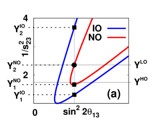
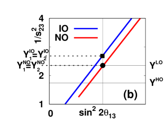
Figure 2: Parameter degeneracy after $\theta_{13}$ was determined, assuming that the true mass ordering is normal and the true $\theta_{23}$ lies in the lower octant. The red (blue) curve corresponds to the case where the test mass ordering is normal (inverted). The true solution is depicted as a black circle, whereas the fake solutions are marked by a black square. In case (a), away from the oscillation maximum, the combination of the quadratic curves through the appearance probabilities ((i) in Eq. (3)) and the line $X=\sin^{2}2\theta_{13}=$ const. ((ii) in Eq. (3)) results in four solutions $Y_{1}^{\scriptsize{\mbox{\rm NO}}}$, $Y_{2}^{\scriptsize{\mbox{\rm NO}}}$, $Y_{1}^{\scriptsize{\mbox{\rm IO}}}$, $Y_{2}^{\scriptsize{\mbox{\rm IO}}}$. In case (b), at the oscillation maximum, the merging of the straight lines ((iii) in Eq. (23)) using the appearance probabilities ((i) in Eq. (3)) and $X=\sin^{2}2\theta_{13}=$ const. ((ii) in Eq. (3)) leads to two (two-fold) degenerate solutions $Y_{1}^{\scriptsize{\mbox{\rm MO}}}=Y_{2}^{\scriptsize{\mbox{\rm MO}}}$ (MO=NO, IO), where MO stands for mass ordering.

In the energy region away from the oscillation maximum, as illustrated in Fig. 2 (a), there are four intersections, $(X,Y)=(\sin^{2}2\theta_{13}^{\,\scriptsize{\mbox{\rm true}}},Y_{j}^{\scriptsize{\mbox{\rm MO}}})~{}(j=1,2$; MO=NO, IO), between the $X=\sin^{2}2\theta_{13}^{\,\scriptsize{\mbox{\rm true}}}$ and the two quadratic curves. Namely, by imposing the conditions (i) in Eq. (3) and (ii) in Eq. (3), the possible solutions for $1/s_{23}^{2}$ are $Y_{1}^{\scriptsize{\mbox{\rm NO}}}$, $Y_{2}^{\scriptsize{\mbox{\rm NO}}}$, $Y_{1}^{\scriptsize{\mbox{\rm IO}}}$, $Y_{2}^{\scriptsize{\mbox{\rm IO}}}$. Furthermore, by combining the condition (iii) in Eq. (23) which implies that $1/s_{23}^{2}$ is either $Y^{\scriptsize{\mbox{\rm LO}}}$ or $Y^{\scriptsize{\mbox{\rm HO}}}$ in Fig. 2 (a), we can reject the solutions $1/s_{23}^{2}=Y_{1}^{\scriptsize{\mbox{\rm IO}}}$ and $1/s_{23}^{2}=Y_{2}^{\scriptsize{\mbox{\rm IO}}}$ in a particular case of Fig. 2 (a). This corresponds to the case in which the baseline is sufficiently long to differentiate between the mass orderings, and we can eliminate the wrong mass ordering, which is represented by the blue curve in Fig. 2 (a). However, since the solution $1/s_{23}^{2}=Y_{1}^{\scriptsize{\mbox{\rm NO}}}$ is close to $1/s_{23}^{2}=Y^{\scriptsize{\mbox{\rm HO}}}$ while $1/s_{23}^{2}=Y_{2}^{\scriptsize{\mbox{\rm NO}}}$ is close to $1/s_{23}^{2}=Y^{\scriptsize{\mbox{\rm LO}}}$, the octant degeneracy cannot be solved in this particular example in Fig. 2 (a).

In the energy region at the oscillation maximum, on the other hand, as depicted in Fig. 2 (b), there are two (two-fold degenerate) intersections, $(X,Y)=(\sin^{2}2\theta_{13}^{\,\scriptsize{\mbox{\rm true}}},Y_{1}^{\scriptsize{\mbox{\rm MO}}}=Y_{2}^{\scriptsize{\mbox{\rm MO}}})$ (MO=NO, IO), between the $X=\sin^{2}2\theta_{13}^{\,\scriptsize{\mbox{\rm true}}}$ and the two straight lines. In this case, the two conditions (i) in Eq. (3) and (ii) in Eq. (3) leads the two possible solutions $1/s_{23}^{2}=Y_{j}^{\scriptsize{\mbox{\rm MO}}}~{}(j=1,2$; MO=NO, IO). If these two solutions $1/s_{23}^{2}=Y_{j}^{\scriptsize{\mbox{\rm MO}}}~{}(j=1,2$; MO=NO, IO) are away from the higher octant solution $1/s_{23}^{2}=Y^{\scriptsize{\mbox{\rm HO}}}$, then the higher octant solution is rejected and the octant degeneracy is solved. If the two straight lines generated by the appearance probabilities are too close, i.e., if $Y_{j}^{\scriptsize{\mbox{\rm IO}}}\simeq Y_{j}^{\scriptsize{\mbox{\rm NO}}}$, then it is difficult to distinguish the true and wrong mass orderings. It is the case with T2HK and ESS$\nu$SB, both having relatively shorter baseline lengths.

Fig. 2 is given for a specific value of the neutrino energy and a specific baseline length, and the values of $Y_{1}^{\scriptsize{\mbox{\rm NO}}}$, $Y_{2}^{\scriptsize{\mbox{\rm NO}}}$, $Y_{1}^{\scriptsize{\mbox{\rm IO}}}$, $Y_{2}^{\scriptsize{\mbox{\rm IO}}}$ depend on the neutrino energy $E$. In fact each experiment provides information of $Y_{1}^{\scriptsize{\mbox{\rm NO}}}$, $Y_{2}^{\scriptsize{\mbox{\rm NO}}}$, $Y_{1}^{\scriptsize{\mbox{\rm IO}}}$, $Y_{2}^{\scriptsize{\mbox{\rm IO}}}$ for all the energies from its energy spectrum, and in principle these pieces of information can be combined to find out the correct solution. For that purpose, we need to know the behavior of $Y_{1}^{\scriptsize{\mbox{\rm NO}}}$, $Y_{2}^{\scriptsize{\mbox{\rm NO}}}$, $Y_{1}^{\scriptsize{\mbox{\rm IO}}}$, $Y_{2}^{\scriptsize{\mbox{\rm IO}}}$ across all energies in the spectrum for each experiment. To observe how this degeneracy is solved or persists using the enerygy spectrum, we plot the values of $Y_{1}^{\scriptsize{\mbox{\rm NO}}}$, $Y_{2}^{\scriptsize{\mbox{\rm NO}}}$, $Y_{1}^{\scriptsize{\mbox{\rm IO}}}$, $Y_{2}^{\scriptsize{\mbox{\rm IO}}}$ as a function of neutrino energy for the future long baseline experiments: T2HK, DUNE, T2HKK and ESS$\nu$SB.

To generate these curves, we adopt the following reference values, which correspond to the arithmetic average of the best fit points in Ref. [1] from the three groups, except $\delta$ which we assume a value of $-90^{\circ}$:

MO	$\Delta m_{21}^{2\ \scriptsize{\mbox{\rm true}}}/10^{-5}\mbox{\rm eV}^{2}$	$|\Delta m_{32}^{2\ \scriptsize{\mbox{\rm true}}}|/10^{-3}\mbox{\rm eV}^{2}$	$\theta_{12}^{\,\scriptsize{\mbox{\rm true}}}$	$\theta_{13}^{\,\scriptsize{\mbox{\rm true}}}$	$\theta_{23}^{\,\scriptsize{\mbox{\rm true}}}$	$\delta^{\,\scriptsize{\mbox{\rm true}}}$	$\rho/\mbox{\rm g}\cdot\mbox{\rm cm}^{-3}$
NO	7.43	2.432	$33.9^{\circ}$	$8.49^{\circ}$	$48.1^{\circ}$	$-90^{\circ}$	2.6
IO	7.43	2.496	$33.9^{\circ}$	$8.55^{\circ}$	$48.3^{\circ}$	$-90^{\circ}$	2.6

Table 1: The reference values of the true oscillation parameters utilized to generate plots in this study are provided for both normal (NO) and inverted (IO) mass orderings (MO). We choose a constant density of $\rho$ = 2.6 g/cm³ for all the experiments for the sake of simplicity.

3.1 T2HK

The experiment T2HK [2] features a baseline length of 295 km and employs an off-axis neutrino beam with an approximate energy of 0.6 GeV. T2HK is conducted at energies near the first oscillation maximum. Therefore, for the neutrino energy of 0.6 GeV in T2HK, the situation is similar to that depicted in Fig. 1 (b), where the resolution of the octant degeneracy is expected to be achieved, provided that the difference of the true and wrong values of $1/s^{2}_{23}$, which is obtained from the disappearance oscillation probabilities $P(\nu_{\mu}\to\nu_{\mu})$ and $P(\bar{\nu}_{\mu}\to\bar{\nu}_{\mu})$, is larger than the experimental errors.

The trajectory of the curve derived from Eq. (15) in the ($\sin^{2}2\theta_{13}$, $1/s^{2}_{23}$)-plane is illustrated in Fig. 3. Since we assume $\delta^{\,\scriptsize{\mbox{\rm true}}}=-\pi/2$ as the true value in this paper, if the true mass ordering is normal, then T2HK alone can rule out the possibility of the wrong mass ordering (i.e., inverted ordering) [16]. Consequently, the curves representing the wrong mass ordering, depicted as dashed curves in Fig. 3, are absent in the left panel of Fig. 3. In this case, if we impose the conditions (i) in Eq. (3) (all the solid colored curves in Fig. 3) and (ii) in Eq. (3) (the vertical dashed line in Fig. 3), then we are left with the only unique solution $(X,Y)=(\sin^{2}2\theta_{13}^{\,\scriptsize{\mbox{\rm true}}},Y_{1}^{\scriptsize{\mbox{\rm NO}}})=(\sin^{2}2\theta_{13}^{\,\scriptsize{\mbox{\rm true}}},Y_{2}^{\scriptsize{\mbox{\rm NO}}})=(\sin^{2}2\theta_{13}^{\,\scriptsize{\mbox{\rm true}}},1/\sin^{2}\theta_{23}^{\,\scriptsize{\mbox{\rm true}}})$ for the energy $E$ = 0.5, 0.6 GeV and 0.7 GeV, and the octant degeneracy, whether $Y=Y^{\scriptsize{\mbox{\rm HO}}}=1/\sin^{2}\theta_{23}^{\,\scriptsize{\mbox{\rm true}}}$ (the horizontal solid line in Fig. 3), or $Y=Y^{\scriptsize{\mbox{\rm LO}}}=1/\cos^{2}\theta_{23}^{\,\scriptsize{\mbox{\rm true}}}$ (the horizontal dashed line in Fig. 3), is resolved in the case where the true mass ordering is normal. Conversely, if the true mass ordering is inverted, then T2HK by itself cannot exclude the possibility of the wrong mass ordering, leading to the presence of the dashed curves in the right panel of Fig. 3. In this case, if we impose the conditions (i) in Eq. (3) (all the solid-colored curves as well as all the dashed-colored curves in Fig. 3) and (ii) in Eq. (3) (the vertical dashed line in Fig. 3), then we are left with three possible solutions (for $E$ = 0.6 GeV) or four possible solutions (for $E$ = 0.5, 0.7 GeV). The T2HK experiment provides information of $Y_{1}^{\scriptsize{\mbox{\rm NO}}}$, $Y_{2}^{\scriptsize{\mbox{\rm NO}}}$, $Y_{1}^{\scriptsize{\mbox{\rm IO}}}$, $Y_{2}^{\scriptsize{\mbox{\rm IO}}}$ for the energies $E$ = 0.5, 0.6 GeV, 0.7 GeV from its energy spectrum, and in principle we could combine them to single out the correct solution. However, since all the values of $Y_{1}^{\scriptsize{\mbox{\rm NO}}}$, $Y_{2}^{\scriptsize{\mbox{\rm NO}}}$, $Y_{1}^{\scriptsize{\mbox{\rm IO}}}$, $Y_{2}^{\scriptsize{\mbox{\rm IO}}}$ are approximately equal to the true value $Y^{\scriptsize{\mbox{\rm HO}}}$, it is difficult to pick the correct one. Ultimately, by applying condition (iii) in Eq. (23) (either the horizontal solid line ($Y=Y^{\scriptsize{\mbox{\rm LO}}}$) or the horizontal dotted line ($Y=Y^{\scriptsize{\mbox{\rm HO}}}$) ), we obtain the unique correct solution $Y=Y^{\scriptsize{\mbox{\rm HO}}}$ for each energy $E$. This is because the difference between $Y=Y^{\scriptsize{\mbox{\rm HO}}}$ and $Y=Y^{\scriptsize{\mbox{\rm LO}}}$ is larger than that between $Y=Y_{1}^{\scriptsize{\mbox{\rm IO}}}$ and $Y=Y_{j}^{\scriptsize{\mbox{\rm NO}}}~{}(j=1,2)$ or $Y=Y_{2}^{\scriptsize{\mbox{\rm IO}}}$. Therefore, the octant degeneracy is resolved even in the case where the true mass ordering is inverted.

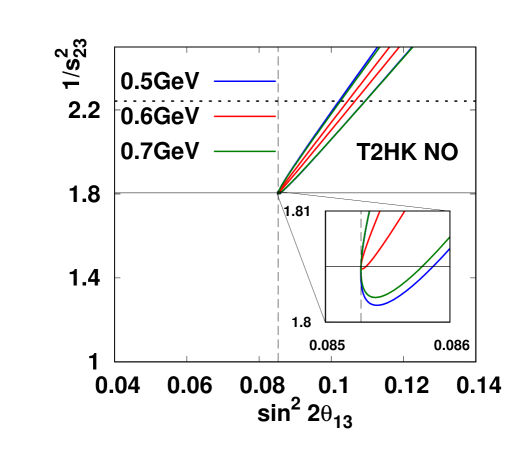
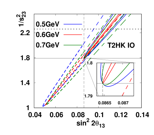
Figure 3: The trajectory of the curve derived by Eq. (15) for the T2HK experiment is illustrated, where a magnified view of the region around $(X,Y)=(\sin^{2}2\theta_{13}^{\,\scriptsize{\mbox{\rm true}}},1/\sin^{2}\theta_{23}^{\,\scriptsize{\mbox{\rm true}}})$ is supplied in each panel. The horizontal thin solid (dotted) straight line represents the true (fake) value $Y=Y^{\scriptsize{\mbox{\rm HO}}}=1/\sin^{2}\theta_{23}^{\,\scriptsize{\mbox{\rm true}}}$ ($Y=Y^{\scriptsize{\mbox{\rm LO}}}=1/\cos^{2}\theta_{23}^{\,\scriptsize{\mbox{\rm true}}}$), whereas the vertical dashed straight line indicates the value of $X=\sin^{2}2\theta_{13}^{\,\scriptsize{\mbox{\rm true}}}$. The left (right) panel corresponds to the case where the true mass ordering is normal (inverted). The solid curves in blue, red and green depict the trajectory of Eq. (15) for neutrino energies of 0.5 GeV, 0.6 GeV and 0.7 GeV, respectively, assuming the true mass ordering. On the other hand, the dashed curves represent trajectories assuming the wrong mass ordering. The energy for the dashed curves corresponds to the energy of the solid curve of the same color. The values of $\theta_{13}^{\,\scriptsize{\mbox{\rm true}}}$ and $\theta_{23}^{\,\scriptsize{\mbox{\rm true}}}$ depend on the true mass ordering as we can see in Table 1.

In general, there are four intersections between the quadratic curves and $X=\sin^{2}2\theta_{13}^{\,\scriptsize{\mbox{\rm true}}}$, as depicted in the left panel of Fig. 2. The values $Y_{1}^{\scriptsize{\mbox{\rm NO}}}$, $Y_{2}^{\scriptsize{\mbox{\rm NO}}}$, $Y_{1}^{\scriptsize{\mbox{\rm IO}}}$, $Y_{2}^{\scriptsize{\mbox{\rm IO}}}$ of these four intersections depend on the neutrino energy $E$. In Fig. 3 the values $Y_{1}^{\scriptsize{\mbox{\rm NO}}}$, $Y_{2}^{\scriptsize{\mbox{\rm NO}}}$, $Y_{1}^{\scriptsize{\mbox{\rm IO}}}$, $Y_{2}^{\scriptsize{\mbox{\rm IO}}}$ are depicted only for $E$ = 0.5 GeV, 0.6 GeV and 0.7 GeV. To observe the behavior of $Y_{1}^{\scriptsize{\mbox{\rm NO}}}$, $Y_{2}^{\scriptsize{\mbox{\rm NO}}}$, $Y_{1}^{\scriptsize{\mbox{\rm IO}}}$, $Y_{2}^{\scriptsize{\mbox{\rm IO}}}$ across all energies in the spectrum, Fig. 4 depicts their values against neutrino energy, spanning the entire range of the energy spectrum. This visualization clarifies the energy dependence of $Y_{1}^{\scriptsize{\mbox{\rm NO}}}$, $Y_{2}^{\scriptsize{\mbox{\rm NO}}}$, $Y_{1}^{\scriptsize{\mbox{\rm IO}}}$, $Y_{2}^{\scriptsize{\mbox{\rm IO}}}$. They are presented for both the cases of normal ordering (left panel: $Y_{1}^{\scriptsize{\mbox{\rm NO}}}$, $Y_{2}^{\scriptsize{\mbox{\rm NO}}}$ for the true mass ordering are in red, whereas $Y_{1}^{\scriptsize{\mbox{\rm IO}}}$, $Y_{2}^{\scriptsize{\mbox{\rm IO}}}$ for the wrong mass ordering are in blue) and inverted ordering (right panel: $Y_{1}^{\scriptsize{\mbox{\rm IO}}}$, $Y_{2}^{\scriptsize{\mbox{\rm IO}}}$ for the true mass ordering are in blue, whereas $Y_{1}^{\scriptsize{\mbox{\rm NO}}}$, $Y_{2}^{\scriptsize{\mbox{\rm NO}}}$ for the wrong mass ordering are in red) as the true mass ordering. The fake value $Y^{\scriptsize{\mbox{\rm LO}}}$ is represented by the horizontal dotted thin line in Fig. 4, whereas the true value $Y^{\scriptsize{\mbox{\rm HO}}}$ is depicted as the horizontal solid line. Notice that $P(E)$ and $\bar{P}(E)$ are calculated using the true values of the oscillation parameters listed in Table 1 for each neutrino energy $E$ and mass ordering. In the energy range of 0.5 GeV $\lesssim E\lesssim$ 0.7 GeV, where there is a substantial number of events for the appearance channels, the discrepancy between the true ($Y_{1}^{\scriptsize{\mbox{\rm MO}}}$) and fake ($Y_{2}^{\scriptsize{\mbox{\rm MO}}}$) solutions is small compared with that between the two octant ($Y^{\scriptsize{\mbox{\rm HO}}}$ and $Y^{\scriptsize{\mbox{\rm LO}}}$) solutions for MO = NO, IO, on the condition that the correct mass ordering is assumed, i.e., $|Y_{2}^{\scriptsize{\mbox{\rm NO}}}-Y_{1}^{\scriptsize{\mbox{\rm NO}}}|\ll|Y^{\scriptsize{\mbox{\rm HO}}}-Y^{\scriptsize{\mbox{\rm LO}}}|$ ($|Y_{2}^{\scriptsize{\mbox{\rm IO}}}-Y_{1}^{\scriptsize{\mbox{\rm IO}}}|\ll|Y^{\scriptsize{\mbox{\rm HO}}}-Y^{\scriptsize{\mbox{\rm LO}}}|$) in the left (right) panel. Therefore, as in Fig. 3, where octant degeneracy was discussed for a given energy, octant degeneracy is expected to be resolved by taking the T2HK energy spectrum into account. We note in passing that, even if the true mass ordering is assumed to be normal (the left panel of Fig. 4), solutions with wrong mass ordering can emerge in lower energy ranges, as indicated by the blue lines. However, the energy in this region is quite low, resulting in a limited number of events.

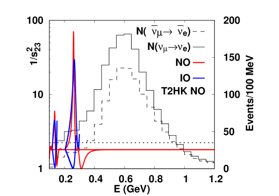
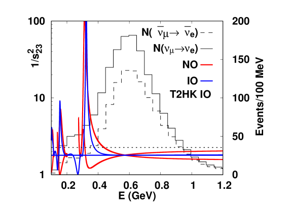
Figure 4: Possible values $Y_{1}^{\scriptsize{\mbox{\rm NO}}}$, $Y_{2}^{\scriptsize{\mbox{\rm NO}}}$, $Y_{1}^{\scriptsize{\mbox{\rm IO}}}$, $Y_{2}^{\scriptsize{\mbox{\rm IO}}}$ for $1/s^{2}_{23}$ are displayed for the case of the true mass ordering being normal (left panel: the two red curves represent $Y_{1}^{\scriptsize{\mbox{\rm NO}}}$, $Y_{2}^{\scriptsize{\mbox{\rm NO}}}$, whereas the two blue curves stand for $Y_{1}^{\scriptsize{\mbox{\rm IO}}}$, $Y_{2}^{\scriptsize{\mbox{\rm IO}}}$) or inverted (right panel: the two blue curves represent $Y_{1}^{\scriptsize{\mbox{\rm IO}}}$, $Y_{2}^{\scriptsize{\mbox{\rm IO}}}$, whereas the two red curves stand for $Y_{1}^{\scriptsize{\mbox{\rm NO}}}$, $Y_{2}^{\scriptsize{\mbox{\rm NO}}}$). There are energy ranges where the solution for the wrong mass ordering does not exist, so the curves for the wrong mass ordering are discontinuous. The horizontal dotted thin straight line represents the fake value $Y=Y^{\scriptsize{\mbox{\rm LO}}}$ of $1/s^{2}_{23}$, whereas the horizontal solid red (blue) line in the left (right) panel stands for the true value $Y=Y^{\scriptsize{\mbox{\rm HO}}}$. Additionally, the expected numbers of events for $\nu_{\mu}\to\nu_{e}$ ($\bar{\nu}_{\mu}\to\bar{\nu}_{e}$), extracted from Ref. [17] under the assumption of $\delta=0$, are included for clarity, enabling a comparison of statistical errors across different energy regions.

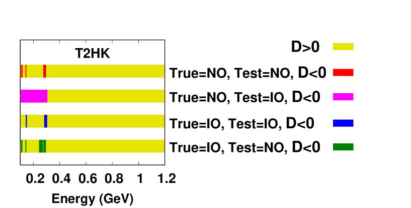
Figure 5: The discriminant $D$ in Eq. (20) for the quadratic curve (15) in the case of the T2HK experiment.

Fig. 5 illustrates the sign of discriminant (20) of the quadratic curve (15) plotted against the neutrino energy in the case of the T2HK experiment. In most of the energy region where the numbers of events of the appearance channels are large, the discriminant is positive, indicating a hyperbolic quadratic curve. Conversely, and at low energies, there are regions where the discriminant becomes negative, resulting in an elliptic quadratic curve.

3.2 DUNE

The DUNE experiment [3] employs a baseline length of 1300 km and utilizes a wideband beam with an average neutrino energy around 2.5 GeV.

The trajectory of the curve described by Eq. (15) for the DUNE experiment is illustrated in Fig. 6. Due to the considerable baseline length, the matter effect at DUNE is significant, which leads to the exclusion of the possibility of a wrong mass ordering by DUNE alone, regardless of the true mass ordering. Although DUNE employs a wideband beam, the situation for the energy range 2.5 GeV $\lesssim E\lesssim$ 3.5 GeV is similar to that at the first oscillation maximum. Fig. 7 presents the values of $Y_{1}^{\scriptsize{\mbox{\rm NO}}}$, $Y_{2}^{\scriptsize{\mbox{\rm NO}}}$, $Y_{1}^{\scriptsize{\mbox{\rm IO}}}$, $Y_{2}^{\scriptsize{\mbox{\rm IO}}}$ for both true and fake solutions as functions of neutrino energy for the whole range of the energy spectrum, in the case of normal ordering (left panel: the solutions for the true mass ordering are $Y_{1}^{\scriptsize{\mbox{\rm NO}}}$, $Y_{2}^{\scriptsize{\mbox{\rm NO}}}$, whereas those for the wrong mass ordering are $Y_{1}^{\scriptsize{\mbox{\rm IO}}}$, $Y_{2}^{\scriptsize{\mbox{\rm IO}}}$) and inverted ordering (right panel: the solutions for the true mass ordering are $Y_{1}^{\scriptsize{\mbox{\rm IO}}}$, $Y_{2}^{\scriptsize{\mbox{\rm IO}}}$, whereas those for the wrong mass ordering are $Y_{1}^{\scriptsize{\mbox{\rm NO}}}$, $Y_{2}^{\scriptsize{\mbox{\rm NO}}}$) as the true mass ordering. In the energy range of 2.5 GeV $\lesssim E\lesssim$ 3.5 GeV, where the number of events of the appearance channels is significant, difference between the true and fake solutions $Y_{1}^{\scriptsize{\mbox{\rm NO}}}$, $Y_{2}^{\scriptsize{\mbox{\rm NO}}}$, $Y_{1}^{\scriptsize{\mbox{\rm IO}}}$, $Y_{2}^{\scriptsize{\mbox{\rm IO}}}$ is minor, suggesting a potential resolution of the octant degeneracy, as long as the difference of the true and wrong values ($Y^{\scriptsize{\mbox{\rm LO}}}$ and $Y^{\scriptsize{\mbox{\rm HO}}}$), derived from the disappearance oscillation probabilities ((iii) in Eq. (23)), exceeds the experimental errors. Similar to the case of T2HK, for DUNE as well, even if the true mass ordering is assumed to be normal, there can be fake solutions in lower energy ranges, as depicted in blue (shown in the left panel of Fig. 7), although the energy in this region is too low to yield a substantial number of events.

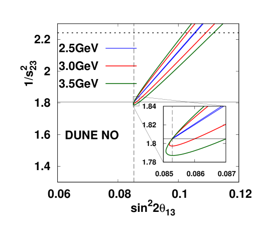
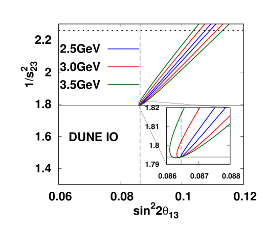
Figure 6: The trajectory of the curve described by Eq. (15) for the DUNE experiment is depicted with a magnified view of the region around $(X,Y)=(\sin^{2}2\theta_{13}^{\,\scriptsize{\mbox{\rm true}}},1/\sin^{2}\theta_{23}^{\,\scriptsize{\mbox{\rm true}}})$. The meaning of the straight thin lines is the same as in Fig. 3. The left (right) panel corresponds to the case of true normal (inverted) mass ordering. The solid curves in blue, red and green represent the trajectory of Eq. (15) for neutrino energy of 2.5 GeV, 3.0 GeV and 3.5 GeV, respectively, assuming that the true mass ordering is normal (inverted) in the left (right) panel.

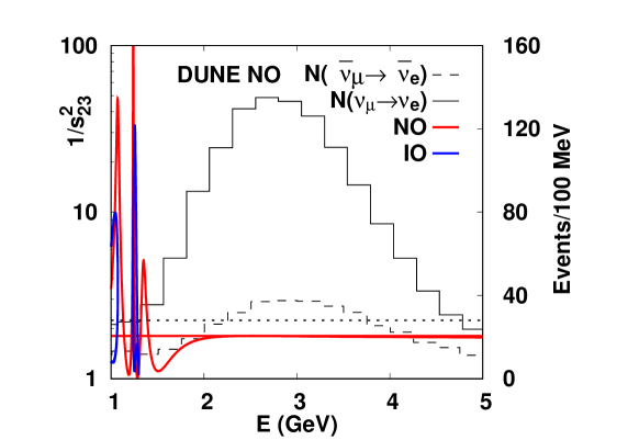
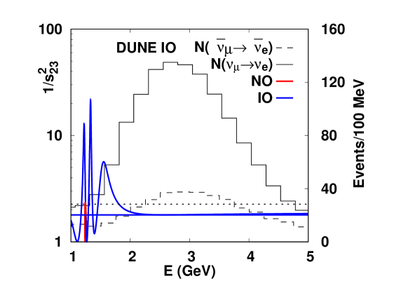
Figure 7: The values of $Y_{1}^{\scriptsize{\mbox{\rm NO}}}$, $Y_{2}^{\scriptsize{\mbox{\rm NO}}}$, $Y_{1}^{\scriptsize{\mbox{\rm IO}}}$, $Y_{2}^{\scriptsize{\mbox{\rm IO}}}$ are depicted for both the true normal (left panel: the two red curves represent $Y_{1}^{\scriptsize{\mbox{\rm NO}}}$, $Y_{2}^{\scriptsize{\mbox{\rm NO}}}$, whereas the two blue curves stand for $Y_{1}^{\scriptsize{\mbox{\rm IO}}}$, $Y_{2}^{\scriptsize{\mbox{\rm IO}}}$) or inverted (right panel: the two red curves represent $Y_{1}^{\scriptsize{\mbox{\rm IO}}}$, $Y_{2}^{\scriptsize{\mbox{\rm IO}}}$, whereas the two blue curves stand for $Y_{1}^{\scriptsize{\mbox{\rm NO}}}$, $Y_{2}^{\scriptsize{\mbox{\rm NO}}}$) mass ordering cases. The meaning of the horizontal straight lines is the same as in Fig. 4. Additionally, the expected numbers of events for $\nu_{\mu}\to\nu_{e}$ ($\bar{\nu}_{\mu}\to\bar{\nu}_{e}$), obtained from Ref. [18], are provided for reference.

Fig. 8 displays the sign of discriminant (20) for the quadratic curve (15) plotted against neutrino energy for the DUNE case. Similarly, in this case, the discriminant is positive for most of the energy region where the number of events of the appearance channels is significant. However, at lower energies, there are regions where the discriminant transitions to negative values.

Figure 8: The discriminant (20) for the quadratic curve (15) in the case of DUNE.

3.3 T2HKK

The T2HKK experiment [13] employs a baseline length of 1100 km and utilizes a wideband beam with an average neutrino energy around 1 GeV. Unlike the T2HK and DUNE experiments, the T2HKK experiment does not cover the energy range at the first oscillation maximum, which occurs at $E=|\Delta m_{31}^{2}|L/(4\times\pi/2)$=2.2 GeV, but rather covers the range at the second oscillation maximum, occurring at $E=|\Delta m_{31}^{2}|L/(4\times 3\pi/2)$=0.75 GeV.

Fig. 9 illustrates the trajectory of the curve described by Eq. (15). Due to the relatively low neutrino energy, the matter effect at T2HKK is not so large and the curves corresponding to the wrong mass ordering appear in both true mass ordering cases. Fig. 9 shows that the difference between the true and fake solutions ($Y_{1}^{\scriptsize{\mbox{\rm MO}}}$ and $Y_{2}^{\scriptsize{\mbox{\rm MO}}}$) is large for each energy and for each mass ordering, giving the impression that it helps to resolve the octant degeneracy. However, the dependence of the location of these intersections on the energy $E$ is so strong that it makes it difficult to resolve the degeneracy, as we will see later.

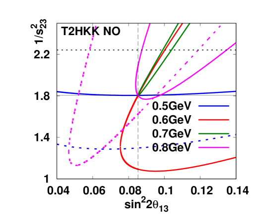
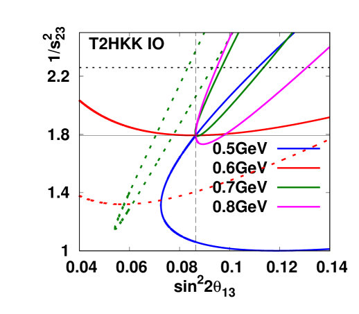
Figure 9: The trajectory traced by the curve described by Eq. (15) for the T2HKK case is showcased. The meaning of the straight thin lines is the same as in Fig. 3. The left (right) panel corresponds to the true normal (inverted) mass ordering. The solid curves colored in blue, red, green and purple denote the trajectory of Eq. (15) for neutrino energy of 0.5 GeV, 0.6 GeV, 0.7 GeV and 0.8 GeV, respectively, assuming the true mass ordering (normal (inverted) ordering in the left (right) panel). Conversely, the dotted curves represent trajectories assuming the wrong mass ordering. The energy value for the dotted curves is the same as that of the solid curve of the corresponding color.

Fig. 10 presents the values of $1/s^{2}_{23}$ for both true and fake solutions as functions of neutrino energy, for the case of normal ordering (left panel: the solutions of $1/s^{2}_{23}$ for the true mass ordering are $Y_{1}^{\scriptsize{\mbox{\rm NO}}}$, $Y_{2}^{\scriptsize{\mbox{\rm NO}}}$, whereas those for the wrong mass ordering are $Y_{1}^{\scriptsize{\mbox{\rm IO}}}$, $Y_{2}^{\scriptsize{\mbox{\rm IO}}}$) and inverted ordering (right panel: the solutions of $1/s^{2}_{23}$ for the true mass ordering are $Y_{1}^{\scriptsize{\mbox{\rm IO}}}$, $Y_{2}^{\scriptsize{\mbox{\rm IO}}}$, whereas those for the wrong mass ordering are $Y_{1}^{\scriptsize{\mbox{\rm NO}}}$, $Y_{2}^{\scriptsize{\mbox{\rm NO}}}$) as the true mass ordering. The behavior of the curves is sensitive to the neutrino energy in the energy range below the first oscillation maximum (i.e., 2.2 GeV). Even in the energy range 0.5 GeV $\lesssim E\lesssim$ 0.8 GeV, where the number of events of the appearance channels is significant, the difference between the values $Y_{1}^{\scriptsize{\mbox{\rm NO}}}$, $Y_{2}^{\scriptsize{\mbox{\rm NO}}}$, $Y_{1}^{\scriptsize{\mbox{\rm IO}}}$, $Y_{2}^{\scriptsize{\mbox{\rm IO}}}$ of $1/s^{2}_{23}$ for true and fake solutions is substantial compared to the difference between the values of the lower ($Y^{\scriptsize{\mbox{\rm LO}}}$) and higher ($Y^{\scriptsize{\mbox{\rm HO}}}$) octant solutions derived from the disappearance channels $\nu_{\mu}\to\nu_{\mu}$ and $\bar{\nu}_{\mu}\to\bar{\nu}_{\mu}$. Furthermore, it is evident that the energy dependence of the difference between the values $Y_{1}^{\scriptsize{\mbox{\rm NO}}}$, $Y_{2}^{\scriptsize{\mbox{\rm NO}}}$, $Y_{1}^{\scriptsize{\mbox{\rm IO}}}$, $Y_{2}^{\scriptsize{\mbox{\rm IO}}}$ of $1/s^{2}_{23}$ for the true and fake solutions is significant. In other words, a slight change in neutrino energy leads to a considerable change in the $1/s^{2}_{23}$ value for both true and fake solutions, causing it to shift from below the correct value to above it. Consequently, integrating this difference over a certain neutrino energy interval yields results that depend on the size of the energy interval, rendering a reliable conclusion difficult to obtain. Hence, it is not expected that the T2HKK experiment alone will resolve the octant degeneracy. It has been previously reported [20] that the detector located at 1100 km in the T2HKK experiment exhibits limited sensitivity to octant degeneracy. The aforementioned discussion regarding the behavior near the second oscillation maximum provides a rationale for the restricted sensitivity observed in T2HKK. However, it is expected that the T2HKK experiment will be combined with the T2HK experiment, which is likely to result in the resolution of the octant degeneracy.

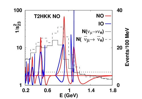
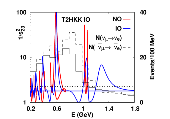
Figure 10: The values $Y_{1}^{\scriptsize{\mbox{\rm NO}}}$, $Y_{2}^{\scriptsize{\mbox{\rm NO}}}$, $Y_{1}^{\scriptsize{\mbox{\rm IO}}}$, $Y_{2}^{\scriptsize{\mbox{\rm IO}}}$ of the two solutions for $1/s^{2}_{23}$ are displayed, with the left panel representing the case of true normal mass ordering and the right panel depicting the true inverted mass ordering case. Similar to Fig. 4, the horizontal dotted thin line indicates the fake value $Y=Y^{\scriptsize{\mbox{\rm LO}}}$ of $1/s^{2}_{23}$ derived from the disappearance oscillation probabilities ((iii) in Eq. (23)), whereas the horizontal solid red (blue) line in the left (right) panel stands for the true value $Y=Y^{\scriptsize{\mbox{\rm HO}}}$. The meaning of the horizontal straight lines is the same as in Fig. 4. For the sake of clarity and to facilitate comparison, the expected numbers of events for $\nu_{\mu}\to\nu_{e}$ ($\bar{\nu}_{\mu}\to\bar{\nu}_{e}$) are provided, sourced from Ref. [13].

Fig. 11 visualizes the sign of the discriminant (20) associated with the quadratic curve (15), portrayed as a function of the neutrino energy for the T2HKK case. Unlike the cases of T2HK and DUNE, even in regions where the number of events in the appearance channels is substantial, the discriminant takes on negative values.

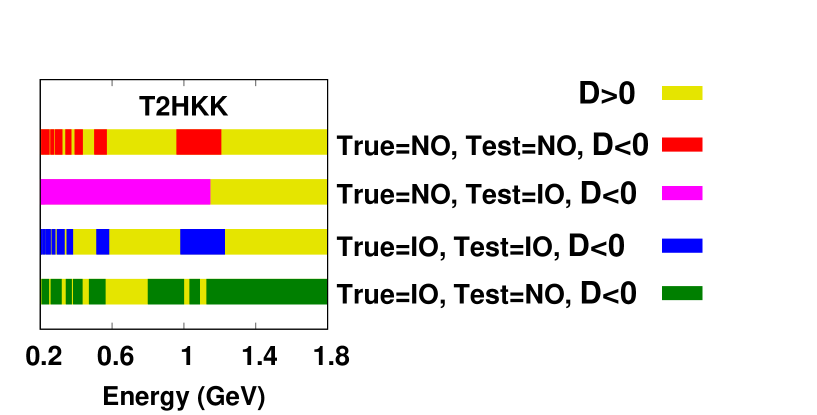
Figure 11: The discriminant (20) for the quadratic curve (15) in the case of T2HKK.

3.4 ESS$\nu$SB

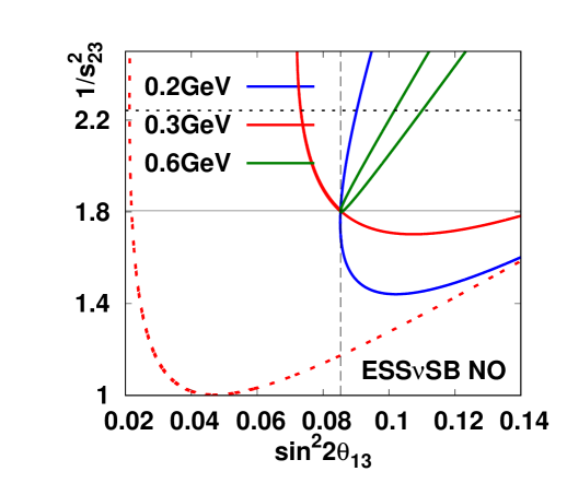
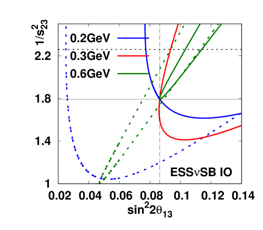
Figure 12: Trajectory of the curve described by Eq. (15) for the ESS$\nu$SB case. The meaning of the straight thin lines is the same as in Fig. 3. The left (right) panel corresponds to the case of true normal (inverted) mass ordering. The solid curves in blue, red and green illustrate the trajectory of Eq. (15) for neutrino energy of 0.2 GeV, 0.3 GeV and 0.6 GeV, respectively, assuming the true mass ordering (normal (inverted) ordering in the left (right) panel).

The ESS$\nu$SB experiment,[14] utilizes a baseline length of 360 km and employs a wideband beam with an average neutrino energy of approximately 0.4 GeV. The ESS$\nu$SB experiment aims to cover energy ranges corresponding to both the first oscillation maximum ($E\sim$ 0.73 GeV) and the second oscillation maximum ($E\sim$ 0.24 GeV).

Fig. 12 illustrates the trajectory of the curve described by Eq. (15). Due to its relatively short baseline length, the matter effect at ESS$\nu$SB is small, and curves corresponding to the wrong mass ordering appear in both true mass orderings. An exception is observed at 0.6 GeV for the true normal mass ordering, where the wrong mass ordering is rejected for the same reason as T2HK. As in the case of T2HKK, Fig. 12 demonstrates that the difference between the true and fake solutions ($Y_{1}^{\scriptsize{\mbox{\rm MO}}}$ and $Y_{2}^{\scriptsize{\mbox{\rm MO}}}$) is significant for each energy and each mass ordering. However, the dependence of the location of these intersections on the energy $E$ is strong.

Fig. 13 illustrates the value of $1/s^{2}_{23}$ for both true and fake solutions, presented as functions of neutrino energy in the case of normal ordering (left panel: the solutions of $1/s^{2}_{23}$ for the true mass ordering are $Y_{1}^{\scriptsize{\mbox{\rm NO}}}$, $Y_{2}^{\scriptsize{\mbox{\rm NO}}}$, whereas those for the wrong mass ordering are $Y_{1}^{\scriptsize{\mbox{\rm IO}}}$, $Y_{2}^{\scriptsize{\mbox{\rm IO}}}$) or inverted one (right panel: the solutions of $1/s^{2}_{23}$ for the true mass ordering are $Y_{1}^{\scriptsize{\mbox{\rm IO}}}$, $Y_{2}^{\scriptsize{\mbox{\rm IO}}}$, whereas those for the wrong mass ordering are $Y_{1}^{\scriptsize{\mbox{\rm NO}}}$, $Y_{2}^{\scriptsize{\mbox{\rm NO}}}$) as the true mass ordering. The behavior of the curves around the energy region of the first oscillation maximum is analogous to that observed in T2HK and DUNE. In this energy range, resolving the octant degeneracy becomes potentially feasible if a substantial number of appearance events are available for both neutrinos and antineutrinos. However, practical observations from Fig. 13 reveal that the numbers of events $N(\bar{\nu}_{\mu}\to\bar{\nu}_{e})$ are relatively low around the energy range corresponding to the first oscillation maximum. Consequently, the resulting larger experimental errors make it challenging to effectively resolve the octant degeneracy. Furthermore, the behavior of the curves around the energy region of the second oscillation maximum resembles that of T2HKK. Octant degeneracy is not likely to be resolved solely using the energy bins around this range. Prior studies [21, 22, 23] have highlighted the limited sensitivity of ESS$\nu$SB to octant degeneracy. The explanations provided above regarding behaviors near the first and second oscillation maxima clarify the reasons for the observed limitations in ability of ESS$\nu$SB to address octant degeneracy.

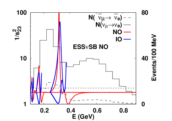
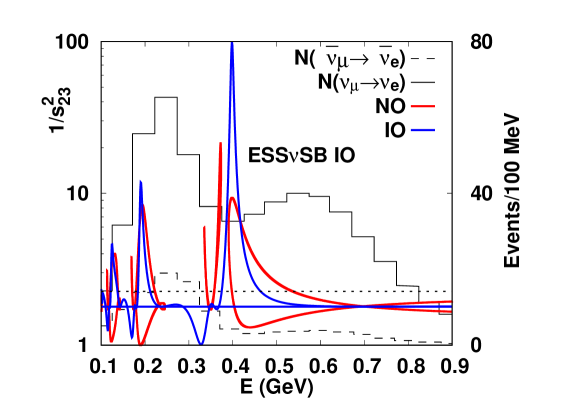
Figure 13: The values of $Y_{1}^{\scriptsize{\mbox{\rm NO}}}$, $Y_{2}^{\scriptsize{\mbox{\rm NO}}}$, $Y_{1}^{\scriptsize{\mbox{\rm IO}}}$, $Y_{2}^{\scriptsize{\mbox{\rm IO}}}$ are shown for the case where the true mass ordering is normal (left panel: the two red curves represent $Y_{1}^{\scriptsize{\mbox{\rm NO}}}$, $Y_{2}^{\scriptsize{\mbox{\rm NO}}}$, whereas the two blue curves stand for $Y_{1}^{\scriptsize{\mbox{\rm IO}}}$, $Y_{2}^{\scriptsize{\mbox{\rm IO}}}$) or inverted (right panel: the two red curves represent $Y_{1}^{\scriptsize{\mbox{\rm IO}}}$, $Y_{2}^{\scriptsize{\mbox{\rm IO}}}$, whereas the two blue curves stand for $Y_{1}^{\scriptsize{\mbox{\rm NO}}}$, $Y_{2}^{\scriptsize{\mbox{\rm NO}}}$). The meaning of the horizontal straight lines is the same as in Fig. 4. Additionally, the expected numbers of events for $\nu_{\mu}\to\nu_{e}$ ($\bar{\nu}_{\mu}\to\bar{\nu}_{e}$), taken from Ref. [19], are provided for reference.

Fig. 14 illustrates the sign of the discriminant (20) for the quadratic curve (15) plotted as a function of the neutrino energy in the case of ESS$\nu$SB. Similar to the cases of T2HK and DUNE, the discriminant remains positive for the energy range around the first oscillation maximum ($E\sim$ 0.73 GeV), while it transitions to negative values around $E\sim$ 0.3 GeV.

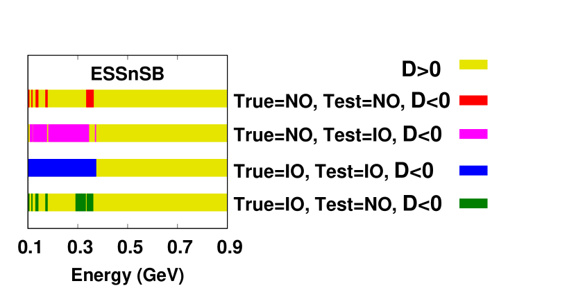
Figure 14: The discriminant (20) of the quadratic curve (15) in the case of ESS$\nu$SB.

From these plots, a general trend emerges suggesting that octant degeneracy can potentially be resolved using energy bins around the first oscillation maximum, assuming sufficiently large numbers of appearance events in this energy range for both neutrinos and antineutrinos. However, it is anticipated to be challenging to effectively address the degeneracy using energy bins centered around the second oscillation maximum.

4 Conclusions

In this paper we conducted an analytical investigation of octant degeneracy after the determination of $\theta_{13}$, utilizing the trajectory defined by the appearance probabilities in the ($\sin^{2}2\theta_{13}$, $1/s^{2}_{23}$)-plane. By considering the appearance channels $\nu_{\mu}\to\nu_{e}$ and $\bar{\nu}_{\mu}\to\bar{\nu}_{e}$, along with the reactor data on $\theta_{13}$, we identified four potential solutions for $1/s^{2}_{23}$. Incorporating the disappearance channels $\nu_{\mu}\to\nu_{\mu}$ and $\bar{\nu}_{\mu}\to\bar{\nu}_{\mu}$, it is theoretically feasible to resolve octant degeneracy, assuming that experimental errors are sufficiently small compared to the difference between the true and fake solutions.

We examined the values of $1/s^{2}_{23}$ for the true and fake solutions in future long baseline experiments, including T2HK, DUNE, T2HKK, and ESS$\nu$SB. T2HK and DUNE have adequate numbers of appearance events for both neutrinos and antineutrinos in the energy region near the first oscillation maximum, where the difference between the values of $1/s^{2}_{23}$ for the true and fake solutions is so minor that the fake octant solution inferred from the disappearance channels can be excluded. As a result, these experiments hold the potential to effectively resolve the octant degeneracy. On the other hand, T2HKK and ESS$\nu$SB encounter challenges due to insufficient numbers of appearance events for either antineutrinos or both neutrinos and antineutrinos around the first oscillation maximum. Moreover, the significant energy-dependent variation between the true and fake solutions around the second oscillation maximum in these experiments makes it difficult to solely overcome the degeneracy through experimental data.

Additionally, we calculated the discriminant of the quadratic curves as a function of energy, illustrating the energy regions where they exhibit hyperbolic or elliptic behavior for each experiment. This aspect was not discussed in Ref.[8].

It is important to note that our study relies on discussions centered around the best-fit points of oscillation parameters. In practice, however, due to experimental errors, conclusions of octant degeneracy resolution should be interpreted with a certain level of confidence in their potential. Our primary aim in this study is to provide analytical insights into which experiments and energy ranges show promise for resolving the octant degeneracy. We hope that our work contributes valuable insights into how octant degeneracy might be addressed in future long baseline experiments.

References

- [1] R. L. Workman et al. [Particle Data Group], PTEP 2022 (2022), 083C01 doi:10.1093/ptep/ptac097
- [2] K. Abe et al. [Hyper-Kamiokande Proto-], PTEP 2015 (2015), 053C02 doi:10.1093/ptep/ptv061 [arXiv:1502.05199 [hep-ex]].
- [3] R. Acciarri et al. [DUNE], [arXiv:1512.06148 [physics.ins-det]].
- [4] G. L. Fogli and E. Lisi, Phys. Rev. D 54, 3667 (1996) [arXiv:hep-ph/9604415].
- [5] J. Burguet-Castell, M. B. Gavela, J. J. Gomez-Cadenas, P. Hernandez and O. Mena, Nucl. Phys. B 608, 301 (2001) [arXiv:hep-ph/0103258].
- [6] H. Minakata and H. Nunokawa, JHEP 0110, 001 (2001) [arXiv:hep-ph/0108085].
- [7] V. Barger, D. Marfatia and K. Whisnant, Phys. Rev. D 65, 073023 (2002) [arXiv:hep-ph/0112119];
- [8] O. Yasuda, New J. Phys. 6 (2004), 83 doi:10.1088/1367-2630/6/1/083 [arXiv:hep-ph/0405005 [hep-ph]].
- [9] Y. Abe et al. [Double Chooz], Phys. Rev. Lett. 108 (2012), 131801 doi:10.1103/PhysRevLett.108.131801 [arXiv:1112.6353 [hep-ex]].
- [10] F. P. An et al. [Daya Bay], Phys. Rev. Lett. 108 (2012), 171803 doi:10.1103/PhysRevLett.108.171803 [arXiv:1203.1669 [hep-ex]].
- [11] J. K. Ahn et al. [RENO], Phys. Rev. Lett. 108 (2012), 191802 doi:10.1103/PhysRevLett.108.191802 [arXiv:1204.0626 [hep-ex]].
-
[12]
I. Esteban, M. C. Gonzalez-Garcia, M. Maltoni, T. Schwetz and A. Zhou,
JHEP 09 (2020), 178
doi:10.1007/JHEP09(2020)178
[arXiv:2007.14792 [hep-ph]];
NuFIT 5.2 (2022), http://www.nu-fit.org/. - [13] K. Abe et al. [Hyper-Kamiokande], PTEP 2018 (2018) no.6, 063C01 doi:10.1093/ptep/pty044 [arXiv:1611.06118 [hep-ex]].
- [14] A. Alekou et al. [ESSnuSB], doi:10.3390/universe9080347 [arXiv:2303.17356 [hep-ex]].
- [15] A. Cervera, A. Donini, M. B. Gavela, J. J. Gomez Cadenas, P. Hernandez, O. Mena and S. Rigolin, Nucl. Phys. B 579, 17 (2000) [Erratum-ibid. B 593, 731 (2000)] [arXiv:hep-ph/0002108].
- [16] S. Prakash, S. K. Raut and S. U. Sankar, Phys. Rev. D 86 (2012), 033012 doi:10.1103/PhysRevD.86.033012 [arXiv:1201.6485 [hep-ph]].
- [17] K. Abe et al. [Hyper-Kamiokande], [arXiv:1805.04163 [physics.ins-det]].
- [18] B. Abi et al. [DUNE], [arXiv:2002.03005 [hep-ex]].
- [19] A. Alekou, E. Baussan, N. B. Kraljevic, M. Blennow, M. Bogomilov, E. Bouquerel, A. Burgman, C. J. Carlile, J. Cederkall and P. Christiansen, et al. [arXiv:2203.08803 [physics.acc-ph]].
- [20] P. Panda, M. Ghosh, P. Mishra and R. Mohanta, Phys. Rev. D 106 (2022) no.7, 073006 doi:10.1103/PhysRevD.106.073006 [arXiv:2206.10320 [hep-ph]].
- [21] S. K. Agarwalla, S. Choubey and S. Prakash, JHEP 12 (2014), 020 doi:10.1007/JHEP12(2014)020 [arXiv:1406.2219 [hep-ph]].
- [22] K. Chakraborty, S. Goswami, C. Gupta and T. Thakore, JHEP 05 (2019), 137 doi:10.1007/JHEP05(2019)137 [arXiv:1902.02963 [hep-ph]].
- [23] A. Alekou et al. [ESSnuSB], Eur. Phys. J. C 81 (2021) no.12, 1130 doi:10.1140/epjc/s10052-021-09845-8 [arXiv:2107.07585 [hep-ex]].