Forecasting with Feedback

Abstract

Systematically biased forecasts are typically interpreted as evidence of forecasters’ irrationality and/or asymmetric loss. In this paper we propose an alternative explanation: when forecasts inform economic policy decisions, and the resulting actions affect the realization of the forecast target itself, forecasts may be optimally biased even under quadratic loss. The result arises in environments in which the forecaster is uncertain about the decision maker’s reaction to the forecast, which is presumably the case in most applications. We illustrate the empirical relevance of our theory by reviewing some stylized properties of Green Book inflation forecasts and relating them to the predictions from our model. Our results point out that the presence of policy feedback poses a challenge to traditional tests of forecast rationality.

Keywords: feedback, biased forecasts, forecast rationality, forecast evaluation, quadratic loss

JEL codes: C53, D82, E37, E58

1 Introduction

It is generally agreed that the main reason why government institutions and private entities engage in forecasting is to improve decision-making. For example, many people use weather forecasts in their daily lives to make decisions that range from the trivial, e.g., whether to go hiking or to the movies, to the more consequential, e.g., whether to evacuate before a storm, or how much to irrigate a field. Weather forecasting is a natural example of a setting in which the decisions made on the basis of the forecast do not directly affect the realized outcome. In the language of our paper, this forecasting-decision environment is free of forecast-induced feedback. When it comes to forecasting some economic variables, on the other hand, the setting is frequently more interactive. Forecasting and decision-making may take place within the same institution and, more importantly, the actions taken in response to the forecast often have an impact on the very outcome that the forecast was meant to predict. The following two examples illustrate environments of this type.

Example 1: The marketing department of a firm produces a sales forecast for a product line for the next fiscal quarter. The managers of the firm have a minimum sales target that they wish to meet. If the sales forecast is substantially below the target, management may decide to take corrective action, such as increasing marketing efforts, offering discounts, etc. These actions are aimed at, and may succeed in, increasing future sales. Hence, the ex-post accuracy of the original forecast may depend on the decisions made in response to it.   

Example 2: Central bank staff inflation forecasts serve a dual role. First, as with any other forecast, they are meant to provide an accurate prediction of realized inflation over some horizon. Second, they also serve as an input for setting the policy rate in a way that guides the economy toward an intermediate or long run inflation target. As rate decisions affect future inflation, forecast performance is hard to judge without accounting for this feedback effect.   

These examples highlight the feedback mechanism that is naturally present in many economic forecasting problems. In these settings some decision makers may follow mechanical decision rules that use forecasts as inputs. Others may be more sophisticated, trying to “invert” forecasts to extract private information known by forecasters, and to act on this information in an optimal way. In either case, if these actions affect the outcome, then one can expect forward-looking forecasters to adjust their forecasts in anticipation of decision makers’ reactions. This type of environment, while common in economic applications, has nonetheless received little attention in the economic forecasting literature. Our research fits into this gap.

More specifically, the goal of this paper is to study the statistical properties of forecasts that are produced in environments with feedback effects. To this end, we present a simple model of the interaction between a forecaster and a decision maker (DM). We concentrate, for simplicity, on the case in which there is a single forecaster and a single DM. We use our model to derive the optimal (equilibrium) forecast, analyze its bias, and provide explicit expressions for the coefficients of the associated Mincer-Zarnowitz (MZ) regression function.

Our theoretical model borrows its basic structure from communication games, pioneered by Crawford and Sobel (1982). In particular, in our model the forecast is interpreted as a message, the forecaster plays the role of the “sender” of the message, and the DM the role of the “receiver” of the message. However, our setup departs from standard models of costless communication such as Crawford and Sobel (1982) in two ways. First, in our model the forecaster’s message (i.e., the forecast) enters his loss function directly, making ours a game of “costly talk,” as in Kartik, Ottaviani, and Squintani (2007). Second, we explicitly model the mechanism by which the state of the economy and the policy action jointly determine the realization of the outcome. This causality is absent in standard communication games, where the realization of the target variable is exogenous.

More concretely, in our model the forecaster uses his private information about the state of the economy to predict the future value of an economic variable, with the objective of minimizing the mean squared error (MSE) of his prediction. The DM observes the forecast and makes a policy decision based on it, designed to steer the realization of the variable toward a given target. This decision may be made optimally, i.e., conditional on the information gleaned from the forecast, or by following a mechanical rule. In either case, the policy action has an impact on the variable that the forecaster was trying to predict. Therefore, the forward-looking forecaster tries to anticipate the DM’s reaction, and account for it in constructing the forecast. However, we also assume (realistically) that the forecaster faces uncertainty about the DM’s objectives. This uncertainty is captured by an uncertain parameter in the DM’s reaction function, and it implies that the forecaster is not able to predict the DM’s reaction perfectly. Policy uncertainty, coupled with forecast-based feedback, are the main drivers of our results, which are as follows.

First, we show that in the presence of feedback and a moderate amount of uncertainty about the DM’s reaction, the optimal (equilibrium) forecast is biased. Furthermore, the intercept and slope of the MZ regression function differ from zero and one, respectively. These properties of equilibrium forecasts in our model are in stark contrast with feedback-free optimal predictions under quadratic loss. Indeed, systematic bias and/or rejection of the null of zero intercept and unit slope by statistical tests has been interpreted as evidence of either forecasters’ irrationality or asymmetric loss. Our analysis suggests that neither conclusion is warranted in the presence of feedback.

Second, we provide analytical formulas for the equilibrium bias and the MZ regression coefficients in terms of the mean and variance of the uncertain parameter in the DM’s reaction function. The absolute value of the bias depends on the degree of uncertainty in the DM’s reaction; a smaller variance shrinks the bias toward zero. In addition, the MZ regression coefficients are shown to be nonlinear functions of the average strength and volatility of the DM’s reaction. The optimal MZ slope can be very flat or even negative, while the intercept is proportional to the DM’s target value for the outcome. In line with the behavior of the bias, the MZ slope converges to one as uncertainty about the DM’s reaction vanishes.

Finally, we provide analogous results in cases where either the DM or the forecaster follows mechanical rules rather than being fully strategic. More specifically, we derive the optimal forecast given that the DM follows a Taylor-rule that takes the forecast at face value or misinterprets the forecast in some other way; and, conversely, we study conditional forecasts based on fixed policy assumptions rather than the anticipation of the DM’s actual reaction. The resulting forecast is generally biased in both cases; we again characterize the bias and the MZ regression coefficients in terms of the average strength and volatility of the DM’s reaction.

The main mechanism behind the results described above is a bias-variance tradeoff. When the forecast is used for policy, the forecaster recognizes that the outcome is a function of the forecast, and uses his knowledge about the DM’s reaction to make a more accurate prediction. However, the DM’s reaction function is such that a higher forecast (in absolute value) induces a stronger reaction to the forecast, which in turn leads to higher volatility in the outcome. Higher outcome volatility is harmful for the forecaster, as it increases the MSE of the forecast, i.e., his expected loss. This problem is resolved optimally by choosing a forecast that is smaller (in absolute value) than the unbiased prediction based on the DM’s expected reaction function. That is, the forecaster mitigates the volatility effect of his forecast by making it less sensitive to his information than the unbiased forecast would be. This modification results in a forecast with lower MSE, but some bias.

Relation to previous literature

The idea that forecasts might alter outcomes has a long history in the social sciences. As an example of early work, Hardt and Mendler-Dünner (2023) point to Morgenstern (1928), who speculated that forecast-induced feedback would necessarily invalidate public forecasts, making prediction in many social settings impossible. This conjecture was later shown to be false by Grunberg and Modigliani (1954) and Simon (1954) in two studies that constitute prequels to the rational expectations literature. In particular, Grunberg and Modigliani (1954) demonstrate the existence of a self-fulfilling forecast in a model of price determination with feedback, while Simon (1954) derives a similar result for election predictions in the presence of “bandwagon” or “underdog” effects.

Decades later, Bowden (1987) used a sequential sampling model to study the convergence of forecasts and outcomes in situations where “publication effects” provide a causal link from the former to the latter. In a follow-up study, Bowden (1989) foreshadows the use of game theory in modeling feedback, but does not give a formal treatment of this idea. Hence, these early frameworks are non-strategic in that the forecaster faces an exogenously given, deterministic reaction function. The formal results then center on showing, via fixed-point theorems, that a self-fulfilling forecast exists. Thus, there is no room or need in these models to study the properties of equilibrium forecasts. By contrast, the reaction function in our model arises endogenously from the optimal behavior of a fully strategic DM and is subject to uncertainty. This setup provides for qualitatively new results.

The interaction between forecasting and decision making has received some attention in the context of how central banks set policy (see Example 1). In a model of professional inflation forecasts and monetary policy, Bernanke and Woodford (1997) study the existence of an informative rational expectations equilibrium (REE). They argue that it may not exist, but do not derive the properties of optimal forecasts in case there is an equilibrium. Faust and Leeper (2005) focus on comparing the information content for the public of conditional and unconditional central bank forecasts—the former type of forecast assumes a fixed policy action, while the latter anticipates the central bank’s optimal reaction to the state of the economy. On the empirical side, Faust and Wright (2008) propose forecast efficiency tests for conditional forecasts, and Knüppel and Schultefrankenfeld (2017) compare inflation forecasts from various central banks with different assumptions about future monetary policy. But neither paper gives a theoretical account of the feedback mechanism and its consequences. Our previous work, Lieli and Nieto-Barthaburu (2020), deals with policy feedback in futures markets; there are analogies between forecasts and prices in that they can both be viewed as signals of agents’ private information. However, ibid. focus on studying the existence of a REE, while the focus here is on the statistical properties of forecasts.

Demonstrating that feedback can generate biased forecasts under quadratic loss and rational behavior is a significant conceptual contribution to the forecast evaluation literature. It is well known that in the absence of feedback, the MSE-optimal forecast is the conditional mean; therefore, the optimal forecast is unbiased, errors are uncorrelated with the forecaster’s information, the MZ slope is unity, etc. The literature has a long history of interpreting violations of these canonical optimality properties as evidence against forecasters’ rationality; see, e.g., Mincer and Zarnowitz (1969), Zarnowitz (1985), Keane and Runkle (1989, 1990), Romer and Romer (2000), Croushore (2012), Patton and Timmermann (2012), Rossi and Sekhposyan (2016), among many others. Another strand of the forecasting literature raises the caveat that forecasts can be optimally biased under asymmetric loss, as in Granger (1969), Elliott, Komunjer, and Timmermann (2005, 2008), Patton and Timmermann (2007), Capistran (2008) and others. Our model goes beyond these traditional narratives, and highlights a specific mechanism—forecast-induced feedback—that can rationally explain such patterns and account for the factors that drive them. We are not aware of other theoretical models that do so.

The rest of the paper proceeds as follows. In Section 2, as motivation for our subsequent analysis, we present some stylized facts related to apparent inefficiencies in Green Book forecasts of inflation. In that section we also discuss the limitations of preference or irrationality based explanations of these facts. In Section 3 we present our model, and provide a thorough discussion of its underlying assumptions. In Section 4 we derive and state our core results on the statistical properties of equilibrium forecasts under feedback. Section 5 revisits the stylized facts related to Green Book forecasts to interpret them through the lens of the model. In Section 6 we discuss an extension of the main model to conditional forecasts. We summarize and state our conclusions in Section 7. All proofs are contained in the Appendix.

2 Empirical motivation

In this section we present some stylized properties of Green Book (GB) inflation forecasts produced by the Federal Reserve staff over several decades. There is little question that feedback should be a relevant consideration in evaluating the properties of GB forecasts, since the Federal Open Market Committee uses these forecasts in formulating monetary policy, which then affects realized inflation in the future (among other economic variables). We demonstrate some remarkable patterns that our theory can speak to, but have been attributed to preferences or irrationality in the existing literature. We highlight and discuss the following two facts:

1. GB inflation forecasts show systematic bias over extended periods, and the sign of the bias shifts over time.

2. The statistical relationship between realized inflation and GB forecasts, as described by the MZ regression, changes gradually over time from the mid-1970s to the mid-2010s, and the overall change is quite radical if we compare the first half of that time period with the second.

Regarding point (i), the influential paper by Romer and Romer (2000) uses MZ regressions on a sample of GB inflation forecasts and realizations from 1965 to 1991 to test for rationality (unbiasedness), and finds no evidence against it. However, in a follow-up study Capistran (2008) convincingly argues that the non-rejection of rationality by Romer and Romer (2000) is due to their overlooking a structural break in the data, where the bias changes sign. Using an extended sample, the top panel of Figure 1 visually confirms this fact. In particular, the figure shows the 40-quarter moving average of the errors associated with 4-quarter-ahead GB inflation forecasts, where we use the latest revision of the GDP deflator as the measure of realized inflation. As it can be seen, persistent bias is a salient feature of GB forecasts. Furthermore, Figure 1 shows that the sign of the bias has shifted again since the study of Capistran (2008).

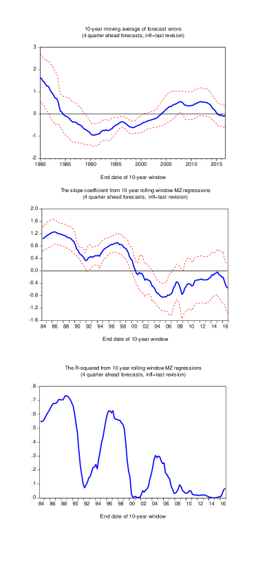
Figure 1: Properties of GB inflation forecasts: bias, MZ slope and MZ R-squared

To our knowledge, stylized fact (ii) has not been documented in the literature. The middle panel of Figure 1 depicts the slope coefficient from a rolling-window MZ regression of realized inflation on the GB forecast over the sample period 1974:q2 through 2016:q4. The forecast horizon is 4 quarters and the window is 40 quarters long. Realized inflation is again taken to be the last revision. The evolution of the slope coefficient is nothing less than striking. It hovers around one from the mid-1980s to the early 1990s and, after a temporary drop, it again returns to unity by the end of the latter decade. However, the relationship between forecast and realization shifts completely in the early 2000s. The slope coefficient dips into significantly negative territory by the middle of the 2000s, and then remains indistinguishable from zero in the last quarter or so of the sample period. The bottom panel of Figure 1 shows the time path of the corresponding R-squared statistic, and demonstrates how the explanatory power of the MZ regression evaporates over time.

While fact (ii) has not been presented in the literature in this form, it is consistent with some reported findings. For example, using an efficiency test applicable in the presence of structural instabilities, Rossi and Sekhposyan (2016) conclude:

“It appears that the [Green Book] forecasts deteriorate over the 1990s and rationality tends to recover by the 2000s. However, for almost all forecast horizons, rationality breaks down again around 2005.” (p. 526)

Thus, ibid. also confirm the shifting nature of GB forecasts using formal statistical tests. However, they interpret the result as a breakdown of rationality.

Capistran (2008) attributes the bias to asymmetries in the Fed’s loss function, and the changes in the sign of the bias to changes in the direction of these asymmetries across monetary policy regimes. While this is certainly possible, the problem with appealing to preference shifts in explaining fact (i) is that this argument can be used to rationalize, ex-post, any change in behavior. Unless one specifies the factors that drive the preference shift, this explanation has little predictive power for the future. On the other hand, labeling fact (ii) as a rationality breakdown also lacks predictive power unless one specifies concrete ways in which behavior might be irrational.

We next develop a formal model which demonstrates that the patterns presented above are consistent with rational forecaster behavior under feedback. We will revisit facts (i) and (ii) in Section 5 and illustrate specifically how our model can be used to interpret them.

3 The model

We present our model in three steps. First, we describe the general forecasting environment. Second, we model the DM’s reaction to the forecast. Third, we discuss in detail the assumptions that we build into the first two steps. A visual summary of the model, in the form of a timeline and an influence diagram, is provided in Appendix A. The reader may find it useful to consult these diagrams at any point during the technical description of the model in Sections 3.1 and 3.2.

3.1 The forecasting environment

We consider the problem of a forecaster who sets out to predict an outcome $y\in\mathbb{R}$ in an environment where the forecast $f$ may affect the realized value of $y$ through actions prompted by the forecast. The forecaster’s information set consists of a private signal $\theta\in\mathbb{R}$, which represents the state of the economy, and is a determinant of $y$. In addition, there is a decision maker (DM) who does not directly observe $\theta$ and relies on the forecast to take an action $a\in\mathbb{R}$, which then also affects the outcome. In particular, we assume that $y$ depends on the state, the action, and a random error $\epsilon$ in a linear way:

$$y=\theta+a+\epsilon.$$ (1)

The error $\epsilon$ is assumed to have zero mean and finite variance $\sigma^{2}>0$, and to be unforecastable in the sense of being independent of $\theta$. The linear specification implies that the DM’s action shifts the conditional mean of $y$ given $\theta$, but not the conditional variance or higher moments.

The forecaster is endowed with a standard quadratic loss function

$$L(y,f)=(y-f)^{2},$$

and his goal is to construct a forecast that minimizes expected loss (mean squared error) conditional on the observed value of $\theta$. Thus, if the forecaster expects the DM to use the reaction function $a=a(f)$, the forecaster’s problem is to solve

$$\min_{f}E[L(y,f)|\,\theta]=\min_{f}E\big{\{}[\theta+a(f)+\epsilon-f]^{2}\mid\theta\big{\}}.$$ (2)

The solution of problem (2) defines the optimal forecast $f^{*}(\theta)$ under the DM’s assumed policy or reaction function.

The fact that we allow the DM to choose her action based on the observed forecast of $y$ introduces the feedback effect that is the focus of our paper. Nevertheless, our framework also nests the traditional model of optimal forecasting with no feedback, in which the outcome is assumed to be exogenous with respect to the forecast. Indeed, one can eliminate feedback in problem (2) by setting $a(f)$ to a constant function, which can then be absorbed into the state $\theta$. It is well known that the optimal forecast in that feedback-free case is given by the conditional mean, i.e., $f^{*}(\theta)=E(y|\,\theta)=\theta$; hence, in that case the optimal forecast is unbiased and the associated forecast errors are uncorrelated with the forecaster’s information. We will show that this is generally not the case in the presence of feedback. Using squared-error loss makes it clear that these canonical optimality properties can be violated without introducing preferences for over- or under-prediction into the model.

It is of course not possible to study problem (2) in full generality without being more specific about the form of the reaction function $a(f)$ and where it comes from. This is the problem we address next.

3.2 The decision maker’s reaction function and the resulting forecasting problem

We equip the DM with a microfounded reaction function. The main building blocks of this foundation are the DM’s objective, and her expectations about how the forecast is constructed. In our general setting, the DM is allowed to be non-strategic in that these expectations — essentially, her interpretation of the forecast — may not be correct. Studying this type of behavioral feedback is still insightful and helps derive the subsequent results under fully rational (strategic) feedback by the DM.

The DM’s objective

We assume that the DM has a target value $y^{T}$ for the outcome, which is common knowledge, and which she tries to achieve by manipulating $a$. The DM’s loss for not hitting the target is a quadratic function of the control error $y-y^{T}$. In addition, the DM faces a quadratic adjustment cost from setting the policy variable to a nonzero value. Hence, the DM’s total ex-post loss from her control problem has the form

$$(y-y^{T})^{2}+ta^{2},$$

where $t\in(-1,\infty)$ is the DM’s adjustment cost parameter. A higher (positive) value of $t$ will dissuade the DM from taking extreme actions to hit the target. Conversely, negative values of the cost parameter correspond to a DM who is prone to overreaction, e.g., for political reasons or because of using the policy action $a$ to fulfill other objectives besides controlling the outcome $y$. Importantly, we assume that the value of $t$ is private information of the DM. (In the language of economic theory, $t$ is the DM’s type.) The forecaster’s beliefs about $t$ are common knowledge. We further assume that $t$ is independent of $(\theta,\epsilon)$.

The DM’s goal is to choose the action $a$ to minimize expected loss conditional on the information conveyed by the forecast. That is, for any given value of the forecast $f$, the DM chooses an action $a$ to solve

$$\min_{a}\big{\{}E[(y-y^{T})^{2}|f]+ta^{2}\big{\}}=\min_{a}\big{\{}E[(\theta+a+\epsilon-y^{T})^{2}|f]+ta^{2}\big{\}},$$

where the expectation is with respect to the distribution of $(\theta,\epsilon)$ given $f$. The following lemma characterizes the solution to this problem.

Lemma 1

The optimal action of the DM is given by

$$a^{*}(f)=\frac{1}{1+t}[y^{T}-E(\theta|f)]:=x[y^{T}-E(\theta|f)],$$ (3)

where $x=1/(1+t)>0$.

The intuition behind Lemma 1 is as follows. The DM wants to steer the outcome $y$ towards her target $y^{T}$. To do so, she must correct exogenous deviations from her target caused by the state. Since she has information about the state given by the forecast, she uses it to compute the optimal policy which, absent adjustment costs, is equal to $y^{T}-E(\theta|f)$. However, given the cost of policy $ta^{2}$, she under- or over-adjusts the outcome by a factor $x=\frac{1}{1+t}\in(0,\infty)$.

DM’s expectations

In order to implement policy rule (3), the DM must make a conjecture about the form of the functional relationship between $\theta$ and $f$, and use it to compute the expectation $E(\theta|f)$. Suppose that the DM conjectures that the forecast is linear in $\theta$; specifically, let $f=b+c\cdot\theta$, $c\neq 0$. Then the conditional expectation in (3) can be computed as

$$E(\theta|f)=\frac{f-b}{c}.$$

Given the way in which the DM forms expectations, her optimal action (3) becomes

$$a^{*}(f)=x\left(y^{T}-\frac{f}{c}+\frac{b}{c}\right).$$ (4)

We will shortly see that the assumption of a linear forecasting rule is self-confirming.

At this point we do not require that the DM-conjectured intercept and slope be equal to the actual intercept and slope used by the forecaster. Instead, in the general case we allow for the DM to be mistaken about the forecaster’s strategy. This generality helps accommodate applications in which policy follows a rigid, mechanical rule. The special case in which the DM’s conjecture is correct constitutes an equilibrium in our model, which we formally define in Section 4. Furthermore, the assumption that the DM conjectures a linear forecast implies that we will be looking for the linear equilibria of our model. We justify this focus in the next subsection.

Example 3: If the DM conjectures $c=1$ and $b=0$, the reaction function (4) reduces to the particularly simple Taylor rule

$$a^{*}(f)=x(y^{T}-f).$$

An interpretation that rationalizes this reaction function is that the DM takes the forecast at “face value” and considers it, somewhat naively, as the state or, equivalently, as the expected outcome given no action ($a=0$). Alternatively, this may be a “pure” behavioral rule without explicit justification. Either way, as we will show, the optimal forecast under this reaction function is not $f(\theta)=\theta$. Therefore, this DM’s conjecture would not be part of an equilibrium.   

The forecaster’s problem

We now return to the forecaster’s problem (2) given the DM’s reaction function (4). As discussed above, the realized value of $x$ is the DM’s private information, and the forecaster knows only the distribution of $x$, which is independent of $(\theta,\epsilon)$. However, we assume that the DM’s conjecture of $(b,c)$ is known to the forecaster; see Section 3.3 below for a detailed justification of these modeling choices. Thus, under the conditions stated above, the forecaster’s problem (2) becomes

$$\min_{f}E\left[\left(\theta+a^{*}(f)+\epsilon-f\right)^{2}|\theta\right]= \min_{f}E\left\{\left[\theta+x\left(y^{T}-\frac{f}{c}+\frac{b}{c}\right)+\epsilon-f\right]^{2}\Bigg{|}\,\theta\right\},$$ (5)

where the expectation is taken w.r.t. the distribution of $(x,\epsilon)$ conditional on $\theta$. Given the maintained independence assumptions, this coincides with the marginal distribution of $(x,\epsilon)$ for any given value of $\theta$. We present and study the solution to problem (5) in Section 4.

3.3 Discussion of modeling assumptions

Outcome determination

A scalar state variable and a linear outcome equation are simplifications that allow us to make our points in a clear and tractable way. In real world applications, such as inflation forecasting, the forecaster’s information set will typically contain observations on many variables. In those cases one might think of $\theta$ as a “sufficient statistic” of the forecaster’s information, or some function of the raw covariates that compresses information (such as, say, a principal component). Moreover, linearity, coupled with the independence of $\theta$ and $\epsilon$, imply that the DM’s action has a direct impact only on the conditional mean $E(y|\,\theta)$ and not on higher moments. Nonetheless, the feedback mechanism described in our model will be present qualitatively even if policy affects the distribution of the outcome in a more complex way.

Forecaster’s preferences

Our choice of the forecaster’s quadratic loss function is deliberate. In the absence of feedback effects, the MSE-optimal forecast is unbiased, and forecast errors are unpredictable given the forecaster’s information. We will show that these properties generally break down under feedback. Using squared-error loss makes it clear that it is the feedback mechanism itself which generates the biases and other non-standard properties of optimal forecasts in our model.

Forecaster’s information

Two key assumptions of the model are that $(i)$ the state is the forecaster’s private information, and $(ii)$ the state cannot be communicated to the DM directly, only through the forecast. We believe that these assumptions capture the main features of forecaster-DM interactions in practice. First, DMs typically rely on advisers because, on their own, they lack the capability or resources to acquire and process all the information relevant to their decisions. Second, for similar reasons, the advice given by experts often comes in the form of summary statistics and projections of key outcomes rather than raw data. Indeed, professional forecasting would be a unnecessary activity if constraints justifying $(ii)$ did not exist in the real world.

DM’s objective and linearity conjecture

A quadratic loss ensures that the DM has an incentive to hit the target on average, and the assumption of a convex adjustment cost is standard throughout the economics literature. Furthermore, we assume that the DM conjectures that the forecast is a linear function of the state. We then look for linear equilibria, where this conjecture is self-confirming. Focusing on linear equilibria is done often in the literature, both for analytical convenience and because linear equilibria are appealing as behavioral predictions. Below we provide conditions for existence and analytically characterize such equilibria.

Interpretation of parameter $x$

We interpret the policy strength parameter $x$ as resulting from the DM optimally resolving the tradeoff between her objectives of controlling outcome $y$ and minimizing the cost of intervention. A more general interpretation of $x$ in (3), which can be divorced from its microfoundation, is that it represents in reduced form the forecaster’s uncertainty about the strength of policy. Such uncertainty can be the result, for instance, of DM-specific idiosyncratic factors that are present at the time of the policy decision. It is reasonable to assume that such information (at least in part) is private to the DM.

Independence of $x$ and $\theta$

The independence of parameter $x$ and the state $\theta$ means that the strength of the policy reaction to the forecast is independent of economic conditions. More generally, it is conceivable that the mean or variance of $x$ could depend on $\theta$; for example, the DM might be expected to react more aggressively during a crisis, and there may be more uncertainty about that reaction in such time. However, there are many possible ways to model this dependence, and it is not obvious what are the salient facts (if any) that should be captured by this additional feature. Therefore, in an abstract model such as ours, independence is a natural benchmark.

Forecaster’s expectations about policy

We assume throughout that the forecaster knows the reaction function $a^{*}(f)$ that governs the DM’s behavior up to the uncertain parameter $x$. It may seem contradictory that $x$ is the DM’s private information while her conjecture about $(b,c)$ is not. This modeling choice can be rationalized in several ways. First, some forecasters, such as those in a central bank, may interact with the DM on a regular basis, and know a lot, but not everything, about her reaction function. As explained above, we use $x$ in our model to represent this residual uncertainty about policy. Second, some DMs may operate under set rules or institutional constraints to interpret forecasts (i.e., choose $b$ and $c$) in a certain way, such as in Example 3.2. Third, the assumption is certainly true in equilibrium, where by definition the DM’s conjecture about $b$ and $c$ coincides with the values actually used by the forecaster. Finally, forecasts derived under a given $(b,c)$ vector can be regarded simply as technical objects that are conditional on the assumed value of $(b,c)$. Even if one questions the empirical relevance of these conditional forecasts, they are still helpful in deriving results about equilibrium forecasts with a fully strategic DM.

Forecaster’s inability to commit

In our model we assume that the forecaster lacks the power to commit to a fixed forecasting rule. We consider this to be a natural assumption, given that the state is not observable directly by the DM, even ex-post. If the forecaster could commit to a set forecasting rule, he could do better than in the no-commitment equilibrium. Such case can be analyzed as a simple extension of our model.

4 Analysis

4.1 Optimal forecasts under feedback

Two key parameters in the determination of the optimal forecast will be the mean and variance of the “strength of policy” variable $x$. Hence, we introduce notation for these parameters: let $\mu:=E(x)>0$ and $\tau^{2}:=var(x)$. The following proposition characterizes the optimal forecast, that is, the forecast that minimizes (5), in terms of these parameters.

Proposition 1

Given the reaction function (4), and the forecaster’s knowledge of $b$ and $c$, the optimal forecast is

$$f^{*}=d^{*}+e^{*}\cdot\theta,$$

where

$$d^{*}=c\left[\frac{\tau^{2}+\mu(\mu+c)}{\tau^{2}+(\mu+c)^{2}}\right]\left(y^{T}+\frac{b}{c}\right),$$ (6)

and

$$e^{*}=c\frac{\mu+c}{\tau^{2}+(\mu+c)^{2}}.$$ (7)

Remarks

1. Proposition 1 shows that the DM’s conjecture of a linear forecast function $f(\theta)$ is self-confirming, i.e., that given such a conjecture, the optimal forecast $f^{*}(\theta)$ is indeed a linear function of $\theta$. Nevertheless, as discussed above, the DM’s guesses about the slope and the intercept of $f^{*}(\theta)$ are allowed to be incorrect. (In fact, it is clear from formulas (6) and (7) that this is generally so for arbitrary $b$ and $c$.) The function $f^{*}(\theta)$ gives the optimal forecast conditional on the DM’s beliefs about forecaster behavior—regardless of whether these beliefs are correct or not.

2. The forecast slope in Proposition 1 is decreasing in the variance of $x$ (in absolute value). That is, the more uncertain the policy reaction to the forecast is, the less responsive is the forecast to the state. The intuition is the following. Since the DM’s action is a function of the forecast, the forecaster correctly anticipates the outcome itself to be a function of the forecast. When uncertainty about the DM’s reaction increases (i.e., when $\tau^{2}$ increases), any given forecast introduces more volatility into the outcome $y$, and that volatility is a component of the forecaster’s MSE loss (see the discussion in Subsection 4.3). However, the forecaster can dampen this volatility by making the forecast lower in absolute value, i.e., by making it less responsive to the state.

As a simple application of Proposition 1, consider a DM acting according to the Taylor rule of Example 3.2.

Example 4: If $c=1$ and $b=0$, i.e., $a^{*}(f)=x(y^{T}-f)$, then $f^{*}=d^{*}+e^{*}\cdot\theta$ with

$$d^{*}=\frac{\tau^{2}+\mu(\mu+1)}{\tau^{2}+(\mu+1)^{2}}y^{T}\;\text{ and }\;e^{*}=\frac{\mu+1}{\tau^{2}+(\mu+1)^{2}}.$$

Thus, we see that the optimal forecast under this naive Taylor rule is not $f(\theta)=\theta$; instead, as explained above, the slope is attenuated toward zero, and the intercept is a fraction of the target. The case in which $\tau^{2}=0$ is also instructive. The optimal forecast is then given by $f^{*}(\theta)=\frac{\mu}{\mu+1}y^{T}+\frac{1}{\mu+1}\theta$. When the forecaster learns $\theta$, he recognizes that it will have both a direct effect on the outcome and an indirect one through the DM’s reaction to the forecast. The optimal forecast accounts for both effects. More formally, the conditional mean of the outcome is $E(y|\,\theta)=\theta+\mu(y^{T}-f)$. The optimal forecast arises by setting this equal to $f$ and then solving for it, i.e., in this case the optimal forecast is unbiased. The case when $\tau^{2}>0$ is more complex, in that the forecaster also cares about how much volatility is introduced into the outcome through the term $-xf$.   

In Example 4.1 the DM is not strategic, in the sense that her interpretation of the forecast is not consistent with how it is actually produced. We can use Proposition 1 to derive the optimal forecast under a fully rational DM’s reaction function. A fully rational DM conjectures the use of a (linear) equilibrium forecast, which we formally define as follows.

Definition 1

A linear equilibrium forecast is a forecast function $f^{\dagger}(\theta)=b^{\dagger}+c^{\dagger}\cdot\theta$ such that if the DM conjectures the use of $f^{\dagger}(\theta)$, then it is optimal for the forecaster to use $f^{\dagger}(\theta)$. More formally, if the DM sets $b=b^{\dagger}$ and $c=c^{\dagger}$ in (4), then $d^{*}=b^{\dagger}$ and $e^{*}=c^{\dagger}$ in Proposition 1.

The equilibrium concept that underlies Definition 1 is pure-strategy Perfect Bayesian Equilibrium (PBE). In equilibrium the forecaster and the DM mutually best-respond to each other, and hold correct (i.e., rational) expectations. The following corollary to Proposition 1 shows that, under some conditions, there are two linear PBE in our model, and it characterizes the equilibrium forecasts when they exist.

Corollary 1

For $\tau^{2}\leq\frac{1}{4}$ there exist two linear PBE with equilibrium forecasts $f^{\dagger}_{i}=b_{i}^{\dagger}+c_{i}^{\dagger}\cdot\theta$, $i=1,2$. The coefficients are as follows.

1. Slopes:

   $$c^{\dagger}_{1}=\frac{1}{2}-\mu+\frac{\sqrt{1-4\cdot\tau^{2}}}{2},$$ (8)

   and

   $$c^{\dagger}_{2}=\frac{1}{2}-\mu-\frac{\sqrt{1-4\cdot\tau^{2}}}{2},$$

   provided that $c^{\dagger}_{1}\neq 0$ and $c^{\dagger}_{2}\neq 0$.

2. Intercepts:

   $$b_{i}^{\dagger}=\frac{k_{i}}{1-k_{i}}c_{i}^{\dagger}\cdot y^{T},$$ (9)

   where

   $$k_{i}=\frac{\tau^{2}+\mu(\mu+c_{i}^{\dagger})}{\tau^{2}+(\mu+c_{i}^{\dagger})^{2}}.$$

Remarks

1. The equilibrium forecast slopes are derived from equation (7) by substituting the common value $c^{\dagger}$ for $c$ and $e^{*}$ and then solving for it. The equilibrium intercepts are then obtained analogously from equation (6).

2. The equilibrium forecasts are one-to-one functions of the state; hence, a rational DM can learn the value of the state from the forecast. That is, the equilibria are separating or fully revealing.

3. If $\tau^{2}>\frac{1}{4}$ an equilibrium does not exist. Indeed, it is easy to verify that if $\tau^{2}>\frac{1}{4}$, then $\frac{\mu+c}{\tau^{2}+(\mu+c)^{2}}<1$ for all values of $c$ and $\mu$. Hence, equation (7) implies that for any slope $c$ conjectured by the DM, the forecaster will always want to use a slope that is attenuated toward zero compared with the DM’s conjecture.

4. If $\operatorname{\emph{supp}}(x)\subset[0,1]$, the condition $\tau^{2}\leq\frac{1}{4}$ is always satisfied. In particular, in that case

   $$\tau^{2}=E(x^{2})-\mu^{2}\leq\mu-\mu^{2}=\mu(1-\mu)\leq\frac{1}{4},$$

   where we have used the fact that $E(x^{2})\leq E(x)$ for a random variable with support in $[0,1]$. More generally, if $x$ is allowed to take values outside the interval $[0,1]$, then $\tau^{2}\leq\frac{1}{4}$ is not guaranteed.

Equilibrium selection

In order to use the model for interpreting observed forecast patterns, we need to take a stance on which equilibrium provides more plausible predictions empirically. We argue that it is the first one for the following reasons:

1. The second equilibrium gives rise to a forecast that decreases in $\theta$ for a larger range parameter values $(\mu,\tau^{2})$ than the first one. In particular, $f^{\dagger}_{2}(\theta)$ decreases in $\theta$ when $\tau^{2}$ is sufficiently close to zero, i.e., when there is little uncertainty. As the outcome depends positively on $\theta$, a forecast function with a negative slope is rather counterintuitive — it is akin to having an inflation forecast that decreases in measures of how overheated the economy is.

2. For a more formal argument, consider the limit of the two equilibria as uncertainty about $x$ vanishes, i.e., as $\tau^{2}\rightarrow 0$ (and so $x\rightarrow_{p}\mu$). As the DM learns the true value of $\theta$ from the forecast in both cases, in the limit the optimal action is $a^{*}=\mu(y^{T}-\theta)$, and the resulting outcome is $y=\theta+\mu(y^{T}-\theta)+\epsilon$. The “natural” optimal forecast of this outcome is then $\theta+\mu(y^{T}-\theta)$, which is indeed the limit of $f_{1}^{\dagger}(\theta)$ as $\tau^{2}\rightarrow 0$. But how can then $\lim f^{\dagger}_{2}(\theta)$ also be an equilibrium forecast? It can be verified that $\lim f^{\dagger}_{2}(\theta)=(1+\mu)y^{T}-\mu\theta$. Thus, expressed in terms of the value of the forecast, the DM reaches the optimal action by adopting the decision rule $a^{*}(f)=f-y^{T}$, as prescribed by (4). But if the DM uses this rule, then the forecaster’s objective (5) becomes completely independent of the forecast. So, he might as well report $f(\theta)=(1+\mu)y^{T}-\mu\theta$ which, in turn, justifies the DM’s decision rule. This is an odd case, in the sense that forecaster behavior in equilibrium rests on the fact that the DM chooses an action that makes the forecaster completely indifferent among all forecasts.

For these reasons, we will choose the first PBE, with slope (8) and intercept (9), as our preferred prediction about behavior in the forecasting game. From now on, we will refer to that equilibrium when deriving the statistical properties of forecasts with feedback.

4.2 The statistical properties of optimal forecasts under feedback

The following proposition characterizes the statistical properties of optimal forecasts in our model, conditional on the DM believing that the forecast function is given by $f(\theta)=b+c\cdot\theta$, $c\neq 0$.

Proposition 2

Let $f^{*}=f^{*}(\theta)$ denote the optimal forecast described in Proposition 1. Then:

1. The optimal forecast is biased, and the bias conditional on the state is given by

   $$E(y-f^{*}|\,\theta)=\frac{\tau^{2}}{\tau^{2}+(\mu+c)^{2}}(\theta-cy^{T}-b).$$ (10)

2. The Mincer-Zarnowitz regression function of the optimal forecast is given by

   $$E(y|f^{*})=-\frac{\tau^{2}}{\mu+c}\left(y^{T}+\frac{b}{c}\right)+\frac{\tau^{2}+c(\mu+c)}{c(\mu+c)}f^{*}.$$ (11)

Remarks

1. Proposition 2 shows that, in general, the statistical properties of optimal forecasts in our model differ from those of optimal forecasts in feedback-free environments. In particular, the optimal forecast is biased (despite the forecaster’s quadratic loss), and the slope of the MZ regression is different from one, implying that the forecast error $y-f^{*}$ is correlated with $f^{*}$. We emphasize that these properties hold even when the DM is fully rational (see Corollary 2 below).

2. The driving force behind the results in Proposition 2 is a combination of two mechanisms: the feedback effect from forecasts to realizations, coupled with the forecaster’s uncertainty about policy strength, i.e., uncertainty about $x$. Indeed, both uncertainty about the DM’s action and feedback from forecasts to policy are needed for the optimal forecast to be biased, as we argue in the next two remarks.

3. To assess the role of uncertainty, one can take the limit $\tau^{2}\to 0$ in equations (10) and (11). It is immediately seen that even in the presence of feedback, when uncertainty about $x$ vanishes, $(i)$ bias vanishes; $(ii)$ the slope of the MZ regression function converges to 1, and $(iii)$ the intercept of that regression function converges to 0. Intuitively, when $\tau^{2}=0$ the DM’s optimal action (4) becomes a fixed, known function of $f$. Hence, a forward-looking forecaster will perfectly anticipate the feedback effect and compensate for it to minimize the MSE of his forecast. Therefore, if there is feedback but no uncertainty about the DM’s action, the properties of optimal forecast in our model coincide with those of feedback-free predictions.

4. To see the effect of policy uncertainty without feedback, suppose that the DM does not rely on the forecast to take action. In this case, the DM’s optimal action is $a^{*}(f)=x[y^{T}-E(\theta)]$, that is, she chooses an adjustment with respect to her unconditional expectation of the state. In turn, the forecaster’s problem is

   $$\min_{f}E[(y-f)^{2}|\,\theta]=\min_{f}E\{[\theta+x(y^{T}-E(\theta))+\epsilon-f]^{2}|\,\theta\}.$$

   This is then a perfectly standard prediction problem whose solution is the conditional mean $f^{*}(\theta)=E(y|\,\theta)=\theta+\mu[y^{T}-E(\theta)]$. Thus, in this feedback-free scenario uncertainty about the action will add to the volatility of forecast errors, but will not cause bias.

As indicated above, the statistical properties of equilibrium forecasts can easily be derived from Proposition 2 by requiring that DM’s conjectures are correct. In Corollary 2 we state these properties for the preferred (first) equilibrium forecast of Corollary 1. In addition, Corollary 2 also specializes Proposition 2 to the case of the simple Taylor rule presented in Example 3.2.

Corollary 2

1. Suppose that $\tau^{2}\leq\frac{1}{4}$, and $\mu\neq\frac{1}{2}+\frac{\sqrt{1-4\tau^{2}}}{2}$ (so an equilibrium exists). The conditional bias and MZ regression function of the equilibrium forecast are given by

   1. $$E(y-f^{\dagger}|\,\theta)=\frac{2\tau^{2}}{1+\sqrt{1-4\tau^{2}}}(\theta-y^{T});$$ (12)

   2. $$E(y|f^{\dagger})=\frac{\tau^{2}}{\tau^{2}-(1-\mu)\left(\frac{1}{2}+\frac{\sqrt{1-4\cdot\tau^{2}}}{2}\right)}y^{T}+\frac{(1-\mu)\left(\frac{1}{2}+\frac{\sqrt{1-4\cdot\tau^{2}}}{2}\right)}{(1-\mu)\left(\frac{1}{2}+\frac{\sqrt{1-4\cdot\tau^{2}}}{2}\right)-\tau^{2}}f^{\dagger}.$$

2. If the DM adopts the simple Taylor rule $a(f)=x(y^{T}-f)$, then the conditional bias and MZ regression function of the optimal forecast are given by

   1. $E(y-f^{*}|\,\theta)=\frac{\tau^{2}}{\tau^{2}+(\mu+1)^{2}}(\theta-y^{T})$;

   2. $E(y|f^{*})=-\frac{\tau^{2}}{\mu+1}y^{T}+\frac{\tau^{2}+\mu+1}{\mu+1}f^{*}$.

Remarks

1. Corollary 2 shows that in general the equilibrium MZ intercept and slope are nonlinear functions of $\mu$ and $\tau^{2}$, as shown by Figures 2 and 3.

2. When $\mu=1$, the MZ slope of the equilibrium forecast is zero, and the MZ intercept is $y^{T}$. To gain some intuition for these results, we need to reinterpret the MZ regression function in the context of feedback. In particular, when the DM chooses her policy actions as a function of the forecast, the outcome itself becomes a function of the forecast. Therefore, the MZ regression is no longer a purely predictive relationship; it becomes “causal” in the sense that different values of the announced forecast will lead to different realizations of the outcome (on average). Now, in equilibrium, a rational DM learns the exact value of the state from the forecast and uses it to adjust the outcome toward the target. When $\mu=1$, there is full adjustment on average, i.e., the average value of $y$ will be equal to $y^{T}$ for any value of the forecast, or more formally $E(y|f^{\dagger})=y^{T}$ for all $f^{\dagger}$. Note however, that this result is rather fragile in the sense that even a relatively small deviation of $\mu$ from unity can induce a large positive or negative MZ slope.

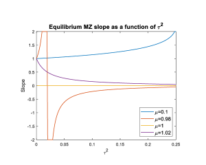
Figure 2: The MZ slope of the equilibrium forecast as a function of $\tau^{2}$ for various values of $\mu$ (functions truncated at 2 and $-2$)

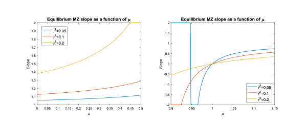
Figure 3: The MZ slope of the equilibrium forecast as a function of $\tau^{2}$ for various values of $\mu$ (functions truncated at $2$ and $-2$; $\mu$-axis also truncated)

4.3 Bias-variance analysis of optimal forecasts under feedback

To highlight the intuition for why the forecaster chooses a biased forecast in the presence of feedback and uncertainty about the policy response, consider the following decomposition of the forecaster’s MSE objective into the sum of the conditional volatility of the outcome plus the squared bias of the forecast:

$$E[(y-f)^{2}|\theta] = E\Big{\{}\big{[}y-E(y|\theta)\big{]}^{2}\big{|}\,\theta\Big{\}}+[E(y|\theta)-f]^{2}$$ (13)

$$= Var(y|\theta)+bias^{2}(f|\theta)$$

$$= Var[a^{*}(f)|\theta]+\big{\{}\theta+E[a^{*}(f)|\theta]-f\big{\}}^{2}+\sigma^{2},$$

where the last equality uses the outcome equation (1).

If $\tau^{2}=0$, then the DM’s reaction function (4) is deterministic with $x=\mu$, and so $Var[a^{*}(f)|\theta]=0$ and $E[a^{*}(f)|\theta]=a^{*}(f)$. Hence, in the absence of policy uncertainty, the first term in (13) vanishes and, as discussed above, the optimal forecast simply drives the bias term to zero. The interpretation is that once the DM’s response to the forecast is perfectly foreseeable, the optimal (equilibrium) forecast will correct for it in full.

By contrast, if the policy parameter $x$ has positive variance, then $Var[a^{*}(f)|\theta]>0$, giving rise to a non-trivial bias-variance tradeoff in (13). That is, the forecaster recognizes that the choice of the forecast contributes to the overall MSE not only through its systematic error but also through the volatility of the outcome, since the outcome depends on the reaction function $a^{*}(f)$, and hence on the forecast. In general, the optimal resolution of this tradeoff calls for manipulating the DM’s action through the forecast in a way that causes the optimal forecast to be systematically biased.

To make this tradeoff more explicit, we can use expression (4) and the mutual independence of $\theta$, $\epsilon$ and $x$ to express the terms in (13) as a function of model primitives:

$$Var(y|\,\theta)=Var\left(\theta+a^{*}(f)+\epsilon\Big{|}\,\theta\right)=Var\left[x\left(y^{T}-\frac{f}{c}+\frac{b}{c}\right)\Big{|}\,\theta\right]+\sigma^{2}$$

$$\quad=Var(x|\,\theta)\left(y^{T}-\frac{f}{c}+\frac{b}{c}\right)^{2}+\sigma^{2}=\tau^{2}\left(y^{T}-\frac{f}{c}+\frac{b}{c}\right)^{2}+\sigma^{2}$$ (14)

and

$$bias^{2}(f|\,\theta)=\left\{E[\theta+a^{*}(f)+\epsilon\big{|}\,\theta]-f\right\}^{2}=\left\{\theta+E\left[x\left(y^{T}-\frac{f}{c}+\frac{b}{c}\right)\Big{|}\,\theta\right]-f\right\}^{2}$$

$$\quad=\left\{\theta+E(x|\,\theta)\left(y^{T}-\frac{f}{c}+\frac{b}{c}\right)-f\right\}^{2}=\left\{\theta+\mu\Big{(}y^{T}+\frac{b}{c}\Big{)}-\Big{(}\frac{\mu+c}{c}\Big{)}f\right\}^{2}.$$ (15)

The variance-bias tradeoff that the forecaster faces is clear from considering equations (14) and (15). The forecaster could choose a forecast function $f(\theta)$ that reduces bias to zero; in particular, the unbiased forecast requires a slope of

$$e=\frac{c}{\mu+c},$$

and an intercept of

$$d=\left(\frac{c}{\mu+c}\right)\left[\mu\left(y^{T}+\frac{b}{c}\right)\right].$$

However, the optimal forecast is different from the unbiased forecast because the variance of the outcome, i.e., equation (14), also depends on the forecast due to the feedback through $a^{*}(f)$. More specifically, we can write the optimal forecast slope (7) as

$$\frac{c(\mu+c)}{\tau^{2}+(\mu+c)^{2}}=\lambda\cdot\frac{c}{\mu+c},$$

where $\lambda=(\mu+c)^{2}/[\tau^{2}+(\mu+c)^{2}]\in(0,1)$. Hence, we can see that the forecaster tries to reduce the volatility of the outcome by attenuating the unbiased forecast slope toward zero. This reduces the sensitivity of the forecast to $\theta$, which in turn mitigates the volatility of the policy response when the state of the economy, and hence the forecast, changes. The cost of this manipulation is the introduction of systematic errors into the forecast.

5 Interpreting the properties of GB forecasts

We want to employ the predictions from our model to interpret the stylized facts presented in Section 2. A prerequisite for this exercise is to argue that GB inflation forecasts are an example of the type of predictions considered in our model. The potential counterargument is that GB forecasts are often seen as being conditioned on a given policy stance (i.e., a given interest rate path), rather than strategically anticipating the FOMC’s response. However, a careful reading of the literature paints a more nuanced picture.

On the nature of GB inflation forecasts

Reifschneider, Stockton, and Wilcox (1997) give a detailed, though perhaps somewhat dated, account of the GB forecast production process. The starting point is indeed a forecast conditioned on a policy stance regarded, in some sense, as “neutral.” This could be a constant interest rate assumption at the current level, but according to Reifschneider and Tulip (2008), historically “[m]ore typical … were paths that modestly rose or fell over time; these trajectories were chosen to signal the staff’s assessment that macroeconomic stability would eventually require some adjustment in policy.” Though ibid. warn that “these conditioning paths may not have represented the staff’s best guess for monetary policy,” in our view this practice can still be interpreted as a cautious attempt to anticipate or endogenize the policy response to the forecast. Perhaps even more importantly, Reifschneider, Stockton, and Wilcox (1997) emphasize that while GB forecasts are informed by various formal models of the economy, the final figures always involve judgemental adjustments. We contend that if these judgements are based in part on qualitative information about future monetary policy, the original conditioning assumption may lose its meaning.

Further support for “unconditionality” is provided by studies documenting the superiority of GB inflation forecasts over alternative predictions such as those appearing in the Survey of Professional Forecasters (SPF) or issued by FOMC members. SPF forecasts are clearly unconditional—agents outside the central bank should incorporate into their prediction their best guess of what the policy maker intends to do given all available information. Similarly, FOMC members are instructed to provide forecasts under what they deem to be “appropriate monetary policy” under the circumstances; see, e.g., McCracken (2010). Still, Sims (2002), Romer and Romer (2008), and Rossi and Sekhposyan (2016) all find that GB forecasts have a clear information advantage over SPF or FOMC forecasts. Sims (2002) concludes that

“these results [are] consistent with a view that the superiority of the Fed forecasts arises from the Fed having an advantage in the timing of information—even with the view that this might arise entirely from the Fed having advance knowledge of its own policy intentions [emphasis added].”

It is not straightforward to rationalize how rigidly conditioned forecasts could outperform forward-looking ones. That is, the superiority of GB forecasts over clearly unconditional competitors over time is support for regarding GB forecasts as unconditional rather than strictly conditional.

Model predictions vs. empirical properties of GB forecasts

We now discuss how the empirical properties of GB forecasts, as shown on Figure 1 in Section 2, can be interpreted through the lens of the theoretical results derived in Corollary 2.

First, our model is capable of generating sign-changing bias (stylized fact (i)) through sign changes in $\theta-y^{T}$. In the context of inflation forecasting, this quantity could be interpreted as a measure of how current economic conditions relate to the level of inflation the Fed targets or considers acceptable. If, in the absence of further intervention or shocks, conditions are loose so that inflation is set to be higher than the target, then the expected equilibrium forecast error is positive, i.e., the forecaster tends to underpredict. This follows from the fact that the multiplier relating $\theta-y^{T}$ to the equilibrium bias is positive (see equation (12)). Conversely, if current conditions are tight so that inflation is set to be below target without further policy changes, then the forecaster tends to overpredict. The former situation (with positive errors) might have been characteristic of the high inflation scenario of the 1970s, and the latter (with negative errors) of the 1980s when there was an initial overtightening in the Volcker-era at the beginning of the decade. Nevertheless, we point out that these interpretations are necessarily vague, since our abstract model is not specific about the empirical content of the state $\theta$.

Second, as Figures 2 and 3 show, the model is capable of generating a wide range of values for the MZ slope depending on the values of parameters $\mu$ and $\tau^{2}$. Using the interpretation of these parameters, one can tell various stories about stylized fact (ii)— the gradual flattening of the MZ slope by the end of the 1990s, its turning negative in the early 2000s, and becoming essentially zero after 2010.

The broad interpretation of parameter $\mu$ in this context is that it measures the aggressiveness with which the Fed pursues its inflation target. A value of $\mu$ close to one would indicate that the Fed is prepared to use whatever rate hike is necessary to achieve its target over a short period, while a low value of $\mu$ means that the Fed is very conscious of the costs of doing so and prefers more cautious adjustments. On the other hand, parameter $\tau^{2}$ measures how predictable is the Fed with regards to its interest rate policy. A larger value of $\tau^{2}$ means that there is high uncertainty about upcoming interest rate decisions. That could indicate, for instance, that there is a lot of disagreement in the FOMC resulting in wider swings in the actions taken. By contrast, a lower $\tau^{2}$ means that the Fed is very clearly committed to a given monetary policy stance — there is not much uncertainty about what they intend to do.

In light of these interpretations, one can formulate several hypotheses about the evolution of the MZ slope.

• As Figure 2 shows, if the Fed is initially reluctant to fight inflation (e.g. $\mu$ is around 0.1), but then switches to a policy of aggressively fighting it ($\mu$ around 1), then we would expect to see a flattening of the MZ slope provided that uncertainty is above a fairly low threshold (say, $\tau^{2}\geq 0.05)$. Moreover, once $\mu$ is close to one, it is easy for the MZ slope to fluctuate around zero and take on negative values as well (this happens when $\mu$ is slightly below one).

• Figure 2 also shows that once $\mu$ is sufficiently close to 1, and there is already a moderate level of uncertainty, then further increases in $\tau^{2}$ attenuate the MZ slope to zero.

• There can be other institutional reasons for the flattening of the MZ slope. As Corollary 2 shows, if the Fed reacts to the forecast mechanically using a simple Taylor rule, then the MZ slope is greater than 1 for all values of $\mu$ and $\tau^{2}$. However, if the Fed starts behaving more strategically (i.e., tries to glean the underlying information about $\theta$ from the forecast), then the forecast production process also changes, and the equilibrium forecast can have a flatter slope (and may switch sign) for the same values of $\mu$ and $\tau^{2}$. For example, if $\mu=0.98$ and $\tau^{2}=0.1$, then the MZ slope under the Taylor rule is 1.05, while the equilibrium (i.e., strategic) slope is $-0.22$.

Of course, our simple model cannot, and does not, capture the Fed’s monetary policy and forecast production processes in all their complexity. The main point we want to make here is that the model is capable of generating meaningful and testable narratives about the observed properties of GB forecasts, which is an appealing alternative to the black box explanations of (changing) preferences or irrationality. Furthermore, there is a substantial empirical literature on monetary policy in the US, which documents several changes in the monetary policy regime from the 1970s to the 2000s using dynamic macroeconomic models. While these models are much more complex than ours, they presumably contain parameters that could be mapped into plausible values for $\mu$ and $\tau^{2}$ over different time periods, opening the door for a more formal empirical validation of the types of hypotheses stated above. We leave this exercise for future research.

6 Extension: conditional forecasts

Motivated by the discussion in Section 5 on the distinction between unconditional and conditional predictions, we now consider an extension of our forecasting model to conditional forecasts, i.e., forecasts made under a fixed (possibly counterfactual) value of the policy action. For example, the staff of some central banks may produce a collection of such forecasts under different policy scenarios. Assuming a fixed policy action means that the forecaster does not try to anticipate the response of the DM to his prediction. Hence, such forecasts will be produced only if the forecaster is not fully rational, or if he follows an institutional mandate to do so. We distinguish between two cases, depending on whether the DM’s reaction to the forecast is unconstrained or is restricted to a pre-specified menu of choices. It is the latter case in which the production of conditional forecasts makes more sense.

6.1 Unconstrained DM

Denote by $a_{0}$ the assumed fixed policy action. Given this action, the outcome would be

$$y=\theta+a_{0}+\epsilon.$$

It is easy to see then that an MSE-minimizer forecaster would choose

$$f^{*}(\theta)=\theta+a_{0},$$ (16)

which is just the expectation of $y$ conditional on $\theta$ and the action being $a_{0}$. If the DM believes that the forecast is of the form $f=b+c\cdot\theta$, her optimal reaction to it is given by the same formula as before:

$$a^{*}(f)=x\left(y^{T}-\frac{f}{c}+\frac{b}{c}\right).$$

In Proposition 3 we state the statistical properties of the conditional forecast (16).

Proposition 3

1. Conditional forecasts are biased, with conditional bias given by

   $$E(y-f^{*}|\theta)=\mu\left(y^{T}+\frac{b}{c}\right)-\left(\frac{\mu+c}{c}\right)a_{0}-\frac{\mu}{c}\theta.$$

2. The MZ regression function of the the conditional forecast is

   $$E(y|f^{*})=-a_{0}+\mu\left(y^{T}+\frac{b}{c}\right)-\left(\frac{\mu-c}{c}\right)f^{*}.$$

Proposition 3 states the properties of conditional forecasts under any assumption that the DM may make about the intercept and slope of the forecasting function. The next corollary states those properties for two special cases of interest: a fully rational DM, who inverts the conditional forecast and chooses her action optimally given the state, and a DM who follows a pure Taylor rule. In the notation of our model, the former uses the correct forecast intercept and slope, $b=a_{0}$ and $c=1$ respectively, and therefore chooses a policy action of the form $a=x(y^{T}-f+a_{0})$; the latter assumes that $b=0$ and $c=1$, and therefore chooses action $a=x(y^{T}-f)$. The expressions for the bias and MZ regression under a fully rational DM and a pure Taylor rule DM follow directly from Proposition 3 by substituting the corresponding values of $b$ and $c$ for each case.

Corollary 3

1. The bias and MZ regression function of a conditional forecast under a fully rational DM are

   1. $E(y-f^{*}|\theta)=-a_{0}+\mu(y^{T}-\theta)$;

   2. $E(y|f^{*})=-(1-\mu)a_{0}+\mu y^{T}+(1-\mu)f^{*}$.

2. The bias and MZ regression function of a conditional forecast under a pure Taylor-rule policy are

   1. $E(y-f^{*}|\theta)=-(\mu+1)a_{0}+\mu(y^{T}-\theta)$;

   2. $E(y|f^{*})=-a_{0}+\mu y^{T}+(1-\mu)f^{*}$.

Remarks

1. Unsurprisingly, conditional forecasts are biased both under the fully rational response and the Taylor rule. The reason is that the forecaster conditions on a counterfactual policy action, i.e., the assumed action generally differs from the one that the DM ultimately implements in response to the forecast. This leads to the forecaster’s using a misspecified model for the outcome determination. We emphasize, however, that in constructing a conditional forecast the forecaster does not face a bias-variance tradeoff, because he does not build the DM’s anticipated reaction into the forecast. This is the reason why the formulas for the bias and the MZ regression coefficients only depend on $\mu$ (the mean of $x$) but not $\tau^{2}$ (the variance of $x$).

2. When $\mu=1$, the MZ regression function under a fully rational policy reaction has slope zero and intercept $y^{T}$. The intuition for this is analogous to the case of an equilibrium forecast with $\mu=1$. As the conditional forecast reveals $\theta$, a rational DM, on average, corrects for the difference between $\theta$ and $y^{T}$ in full (because $\mu=1$). This will produce realizations of $y$ that are, on average, equal to $y^{T}$. In this case the forecast, which is based on a counterfactual policy assumption, becomes completely disassociated from the outcome.

3. When $\mu=1$, the MZ regression function under a pure Taylor rule has slope zero and intercept $-a_{0}+y^{T}$. A DM who follows a pure Taylor rule correctly perceives (either just by chance or by some unmodelled reasoning) that the slope of the forecast is 1, and therefore correctly designs her policy to correct for the state. However, such a DM does not account for the intercept used by the forecaster, coming from the assumed policy underlying the forecast. Hence, this DM systematically misses the target by $-a_{0}$. An alternative Taylor rule of the form $a=a_{0}+x(y^{T}-f)$ would be optimal for the DM who receives a conditional forecast made under the counterfactual policy $a_{0}$.

6.2 Constrained DM

We now consider a situation where the DM is restricted to a pre-specified, fixed menu of choices. For simplicity, let the choice set consist of two actions $\{a_{0},a_{1}\}$; e.g., hold the policy rate or cut it by 25 basis points. The DM instructs the forecaster to produce a vector of conditional forecasts $f=(f_{0},f_{1})$, where $f_{j}$ is to be constructed under the assumption that $a=a_{j}$, $j=0,1$. A forecaster with quadratic loss optimally reports $f_{j}(\theta)=\theta+a_{j}$, which is unbiased when $a=a_{j}$. The DM will choose $a_{0}$ if and only if

$$E[(\theta+a_{0}+\epsilon-y^{T})^{2}|\,f]+ta_{0}^{2}\leq E[(\theta+a_{1}+\epsilon-y^{T})^{2}|\,f]+ta_{1}^{2}$$

$$\Leftrightarrow(f_{0}-y^{T})^{2}+\sigma^{2}+ta_{0}^{2}\leq(f_{1}-y^{T})^{2}+\sigma^{2}+ta_{1}^{2}$$

$$\Leftrightarrow(f_{0}-y^{T})^{2}-(f_{1}-y^{T})^{2}\leq t(a_{1}^{2}-a_{0}^{2}).$$

Thus, if $t=0$, the DM will simply choose the policy scenario for which the conditional forecast is closest to the target in absolute value. More generally, the cost of taking action is also taken into consideration.

In this situation one of the conditional forecasts, the one conditional on the action actually taken, will be unbiased, and will have a MZ regression function with an intercept equal to zero and a slope equal to one. On the other hand, the conditional forecast based on the counterfactual action will be biased. Hence, in evaluating conditional forecasts the extent to which the assumed policy differs from the actually implemented one should be a primary consideration.

7 Conclusion

We present and analyze a model of forecasting in the presence of policy feedback. While empirically relevant, the forecasting literature has largely overlooked this problem. Our paper is an attempt to bridge this gap, by clarifying the consequences of feedback for the properties of forecasts produced under quadratic loss.

Our results show that when feedback effects are present, and there is some degree of uncertainty about the decision maker’s response to the forecast, the canonical properties of mean-square optimal forecasts break down. In particular, forecasts in feedback-prone environments are biased, and forecast errors are predictable given information possessed by the forecaster. Furthermore, the biases become more pronounced when policy uncertainty increases. These properties are in stark contrast to those of mean-squared-optimal forecasts under no feedback.

Given the simple structure of our model, we can explicitly show how the forecast bias and the coefficients of the Mincer-Zarnowitz regression depend on the mean and variance of the uncertain parameter in the decision maker’s reaction function. These detailed results can be used to derive a range of testable predictions about the properties of feedback-prone forecasts in different environments. We illustrate the use of these results by interpreting the historical changes in the properties of Green Book inflation forecasts through the lens of the model. A more formal application of the model to Green Book forecasts is left for future research.

Our results have implications for the literatures concerned with forecast rationality testing and loss function identification from observed data. In particular, our model illustrates that forecast biases can arise from factors other than irrationality or asymmetries in the loss function. Therefore, we argue that forecast evaluation exercises need to either make the identifying assumption of no-feedback (when reasonable), or to think carefully about the feedback mechanism present in the application at hand.

A. Appendix: Model summary

Figure 4: The model’s timeline and influence diagram

B. Appendix: Proofs

Proof of Proposition 1

To facilitate other derivations, it is useful to decompose the forecaster’s conditional MSE (5) into a conditional variance and bias component. In particular,

$$E[(y-f)^{2}|\,\theta]=E\big{[}(y-E(y|\theta))^{2}\big{|}\,\theta\big{]}+(E(y|\theta)-f)^{2}=var(y|\theta)+bias^{2}(f|\theta),$$

where

$$y=\theta+x\left(y^{T}-\frac{f}{c}+\frac{b}{c}\right)+\epsilon.$$ (17)

Equations (15) and (14) in the main text show that

$$var(y|\,\theta)=\tau^{2}\left(y^{T}-\frac{f}{c}+\frac{b}{c}\right)^{2}+\sigma^{2},$$ (18)

and

$$E(y|\,\theta)-f=\theta+\mu\left(y^{T}-\frac{f}{c}+\frac{b}{c}\right)-f=\theta+\mu\left(y^{T}+\frac{b}{c}\right)-\left(\frac{\mu}{c}+1\right)f,$$ (19)

where the variance formula relies heavily on the mutual independence of $x$, $\theta$ and $\epsilon$. Thus, the forecaster’s conditional MSE is given by

$$var(y|\theta)+bias^{2}(f|\theta) = \tau^{2}\left(y^{T}-\frac{f}{c}+\frac{b}{c}\right)^{2}+\sigma^{2}+\left[\theta+\mu\left(y^{T}+\frac{b}{c}\right)-\left(\frac{\mu}{c}+1\right)f\right]^{2}$$ (20)

Setting the partial derivative of (20) w.r.t. $f$ equal to zero results in the FOC:

$$\frac{\tau^{2}}{c}\left(y^{T}-\frac{f}{c}+\frac{b}{c}\right)+\left(\frac{\mu}{c}+1\right)\left[\theta+\mu\left(y^{T}+\frac{b}{c}\right)-\left(\frac{\mu}{c}+1\right)f\right]=0.$$

Solving this linear equation for $f$ yields $f^{*}(\theta)=d^{*}+e^{*}\cdot\theta$, where the slope $e^{*}$ is given by expression (7) and the intercept $d^{*}$ is given by expression (6).  

Proof of Corollary 1

As explained in Remark 1 after Corollary 1, we set

$$c^{\dagger}=\frac{c^{\dagger}(\mu+c^{\dagger})}{\tau^{2}+(\mu+c^{\dagger})^{2}}.$$

Dropping the dagger superscript and rearranging yields the following quadratic equation in $c$:

$$c^{2}+(2\mu-1)c+\mu(\mu-1)+\tau^{2}=0.$$

The quadratic formula then gives:

$$c_{1,2}=\frac{-(2\mu-1)\pm\sqrt{(2\mu-1)^{2}-4(\mu(\mu-1)+\tau^{2})}}{2}=\frac{1}{2}-\mu\pm\frac{1}{2}\sqrt{1-4\tau^{2}},$$

as stated in equation (8). The equilibrium intercept is obtained by substituting the common value $b^{\dagger}$ for $d^{*}$ and $b$ in equation (6) and then solving equation

$$b^{\dagger}=\frac{c\left(y^{T}+\frac{b^{\dagger}}{c}\right)(\tau^{2}+\mu(\mu+c))}{\tau^{2}+(\mu+c)^{2}}$$

for $b^{\dagger}$. This yields expression (9) once $c$ is taken to be $c^{\dagger}_{i}$.   

Proof of Proposition 2

Starting from the bias formula in equation (19) and substituting $f^{*}=d^{*}+e^{*}\cdot\theta$ gives

$$E(y|\,\theta)-f^{*} = \theta+\mu\left(y^{T}+\frac{b}{c}\right)-\left(\frac{\mu}{c}+1\right)(d^{*}+e^{*}\cdot\theta)$$

$$= \mu\left(y^{T}+\frac{b}{c}\right)-\left(\frac{\mu}{c}+1\right)d^{*}+\left[1-e^{*}\left(\frac{\mu}{c}+1\right)\right]\theta.$$

Substituting expression (7) for $e^{*}$ and expression (6) for $d^{*}$ yields

$$E(y|\,\theta)-f^{*}$$

$$=\mu\left(y^{T}+\frac{b}{c}\right)-\left(\frac{\mu}{c}+1\right)c\frac{\tau^{2}+\mu(\mu+c)}{\tau^{2}+(\mu+c)^{2}}\left(y^{T}+\frac{b}{c}\right)+\left[1-\left(\frac{\mu}{c}+1\right)\frac{c(\mu+c)}{\tau^{2}+(\mu+c)^{2}}\right]\theta$$

$$=\left(y^{T}+\frac{b}{c}\right)\frac{-c\tau^{2}}{\tau^{2}+(\mu+c)^{2}}+\frac{\tau^{2}}{\tau^{2}+(\mu+c)^{2}}\theta$$

$$=\frac{\tau^{2}}{\tau^{2}+(\mu+c)^{2}}(\theta-cy^{T}-b),$$

which is the result stated in Proposition 2 part 1.

Turning to the Mincer-Zarnowitz (MZ) regression, one can take the expectation of (17) with respect to $(x,\epsilon)$, conditional on $f=f(\theta)$, to obtain

$$E(y|f)=E(\theta|f)+\mu\left(y^{T}-\frac{f}{c}+\frac{b}{c}\right),$$ (21)

where we used the fact that $f(\theta)$ and $(x,\epsilon)$ are independent (since $\theta$ and $(x,\epsilon)$ are independent). Since in equilibrium the forecast is $f^{*}=d^{*}+e^{*}\theta$, it follows that $E(\theta|f^{*})=f^{*}/e^{*}-d^{*}/e^{*}$. Substituting into (21) gives

$$E(y|f^{*}) = \frac{f^{*}}{e^{*}}-\frac{d^{*}}{e^{*}}+\mu\left(y^{T}-\frac{f^{*}}{c}+\frac{b}{c}\right)=\left(\frac{1}{e^{*}}-\frac{\mu}{c}\right)f^{*}+\mu\left(y^{T}+\frac{b}{c}\right)-\frac{d^{*}}{e^{*}}$$

Further substituting expression (7) for $e^{*}$ and expression (6) for $d^{*}$ yields

$$E(y|f^{*}) = \left(\frac{\tau^{2}+(\mu+c)^{2}}{c(\mu+c)}-\frac{\mu}{c}\right)f^{*}+\mu\left(y^{T}+\frac{b}{c}\right)-\frac{\left(y^{T}+\frac{b}{c}\right)(\tau^{2}+\mu(\mu+c))}{\mu+c}$$

$$= \frac{\tau^{2}+c(\mu+c)}{c(\mu+c)}f^{*}+\left(y^{T}+\frac{b}{c}\right)\left(\mu-\frac{\tau^{2}+\mu(\mu+c)}{\mu+c}\right)$$

$$= -\left(\frac{\tau^{2}}{\mu+c}\right)\left(y^{T}+\frac{b}{c}\right)+\frac{\tau^{2}+c(\mu+c)}{c(\mu+c)}f^{*},$$

as stated in equation (11).   

Proof of Corollary 2

For the equilibrium bias and MZ regression, notice that the equilibrium forecast slope and intercept $c^{\dagger}$ and $b^{\dagger}$ are as in equations (8) and (9), respectively. Substituting the values of $c$ and $d$ in the expressions for the optimal bias and Mincer-Zarnowitz regression (10) and (11) for $c^{\dagger}$ and $b^{\dagger}$ yields the expressions of the equilibrium bias and Mincer-Zarnowitz regressions in part 1 of Corollary 2.

Turning to the bias and MZ regression under a simple Taylor rule policy $a(f)=x(y^{T}-f)$, note that this policy rule is equivalent to the DM conjecturing a forecast intercept $b=0$ and slope $c=1$, and acting optimally conditional on these conjectures. Substituting the values of $c$ and $d$ in the expressions for the optimal bias and Mincer-Zarnowitz regression (10) and (11) for $1$ and $0$ respectively yields the expressions of the bias and Mincer-Zarnowitz regressions under a simple Taylor rule policy in part 2 of Corollary 2.  

Proof of Proposition 3

To compute the conditional bias of conditional forecasts, simply substitute the formula of the optimal conditional forecast (16) into the bias expression (19) to yield

$$E(y|\,\theta)-f^{*}=\theta+\mu\left(y^{T}+\frac{b}{c}\right)-\left(\frac{\mu}{c}+1\right)f^{*}=\theta+\mu\left(y^{T}+\frac{b}{c}\right)-\left(\frac{\mu}{c}+1\right)(\theta+a_{0}).$$

Simple algebra shows that this expression simplifies to (1).

Turning to the MZ regression function, with a conditional forecast $f^{*}=\theta+a_{0}$, we have that $E(\theta|f^{*})=f^{*}-a_{0}$. Substituting into the formula for the MZ regression (21) yields

$$E(y|f)=f^{*}-a_{0}+\mu\left(y^{T}-\frac{f^{*}}{c}+\frac{b}{c}\right).$$

Again, simple algebra shows that this expression simplifies to (2).

References

- (1)
- Bernanke and Woodford (1997) Bernanke, B. S., and M. Woodford (1997): “Inflation forecasts and Monetary Policy,” Journal of Money, Credit and Banking, 29(4), 653–684.
- Bowden (1987) Bowden, R. J. (1987): “Repeated sampling in the presence of publication effects,” Journal of the American Statistical Association, 82(398), 476–484.
- Bowden (1989) (1989): “Feedback forecasting games: an overview,” Journal of Forecasting, 8(2), 117–127.
- Capistran (2008) Capistran, C. (2008): “Bias in Federal Reserve inflation forecasts: Is the Federal Reserve irrational or just cautious?,” Journal of Monetary Economics, 55(8), 1415–1427.
- Crawford and Sobel (1982) Crawford, V. P., and J. Sobel (1982): “Strategic Information Transmission,” Econometrica, 50(6), 1431–1451.
- Croushore (2012) Croushore, D. (2012): “Forecast Bias in Two Dimensions,” Working Paper, Federal Reserve Bank of Philadelphia.
- Elliott, Komunjer, and Timmermann (2005) Elliott, G., I. Komunjer, and A. Timmermann (2005): “Estimation and Testing of Forecast Rationality under Flexible Loss,” The Review of Economic Studies, 72(4), 1107–1125.
- Elliott, Komunjer, and Timmermann (2008) (2008): “Biases in macroeconomic forecasts: irrationality or asymmetric loss?,” Journal of the European Economic Association, 6, 122–157.
- Faust and Leeper (2005) Faust, J., and E. Leeper (2005): “Forecasts and inflation reports: An evaluation,” Mimeo.
- Faust and Wright (2008) Faust, J., and J. H. Wright (2008): “Efficient forecast tests for conditional policy forecasts,” Journal of Econometrics, 146, 293–303.
- Granger (1969) Granger, C. W. (1969): “Prediction with a Generalized Cost Function,” Operational Research, 20, 199–207.
- Granger and Machina (2006) Granger, C. W., and M. J. Machina (2006): “Forecasting and Decision Theory,” Handbook of Economic Forecasting, 1.
- Grunberg and Modigliani (1954) Grunberg, E., and F. Modigliani (1954): “The Predictability of Social Events,” The Journal of Political Economy, 62(6), 465–478.
- Hardt and Mendler-Dünner (2023) Hardt, M., and C. Mendler-Dünner (2023): “Performative Prediction: Past and Future,” arXiv unpublkished manuscript.
- Kartik, Ottaviani, and Squintani (2007) Kartik, N., M. Ottaviani, and F. Squintani (2007): “Credulity, lies, and costly talk,” Journal of Economic Theory, 134, 93–116.
- Keane and Runkle (1989) Keane, M. P., and D. E. Runkle (1989): “Are Economic Forecasts Rational?,” Quarterly Review, 13(2), 26–33.
- Keane and Runkle (1990) (1990): “Testing the Rationality of Price Forecasts: New Evidence from Panel Data,” American Economic Review, 80(4), 714–735.
- Knüppel and Schultefrankenfeld (2017) Knüppel, M., and G. Schultefrankenfeld (2017): “Interest rate assumptions and predictive accuracy of central bank forecasts,” Empirical Economics, 53, 195–215.
- Lieli and Nieto-Barthaburu (2020) Lieli, R. P., and A. Nieto-Barthaburu (2020): “On the Possibility of Informative Equilibria in Futures Markets with Feedback,” Journal of the European Economic Association, 18(3), 1521–1552.
- McCracken (2010) McCracken, M. W. (2010): “Using FOMC forecasts to forecast the economy,” Economic synopses, Federal Reserve Bank of St. Louis, 5, 1–2.
- Mincer and Zarnowitz (1969) Mincer, J., and V. Zarnowitz (1969): The Evaluation of Economic Forecasts. National Bureau of Economic Research, New York.
- Morgenstern (1928) Morgenstern, O. (1928): “Wirtschaftsprognose: Eine Untersuchung ihrer Voraussetzungen und Möglichkeiten,” Springer.
- Nelson and Winter (1964) Nelson, R. R., and S. G. Winter (1964): “A case study in the economics of information and coordination the weather forecasting system,” The Quarterly Journal of Economics, 78(3), 420–441.
- Patton and Timmermann (2007) Patton, A. J., and A. Timmermann (2007): “Testing Forecast Optimality Under Unknown Loss,” Journal of the American Statistical Association, 102(480), 1172–1184.
- Patton and Timmermann (2012) (2012): “Forecast Rationality Tests Based on Multi-Horizon Bounds,” Journal of Business & Economic Statistics, 30(1), 1–17.
- Pesaran and Skouras (2004) Pesaran, M. H., and S. Skouras (2004): “Decision-Based Methods for Forecast Evaluation,” in A Companion to Economic Forecasting, ed. by M. Clements, and D. Hendry, pp. 241–267. John Wiley & Sons, Ltd.