Optimal ratcheting of dividend payout under Brownian motion surplus

Abstract

This paper is concerned with a long standing optimal dividend payout problem in insurance subject to the so-called ratcheting constraint, that is, the dividend payout rate shall be non-decreasing over time. The surplus process is modeled by a drifted Brownian motion process and the aim is to find the optimal dividend ratcheting strategy to maximize the expectation of the total discounted dividend payouts until the ruin time. Due to the path-dependent constraint, the standard control theory cannot be directly applied to tackle the problem. The related Hamilton-Jacobi-Bellman (HJB) equation is a new type of variational inequality. In the literature, it is only shown to have a viscosity solution, which is not strong enough to guarantee the existence of an optimal dividend ratcheting strategy. This paper proposes a novel partial differential equation method to study the HJB equation. We not only prove the the existence and uniqueness of the solution in some stronger functional space, but also prove the monotonicity, boundedness, and $C^{\infty}$-smoothness of the dividend ratcheting free boundary. Based on these results, we eventually derive an optimal dividend ratcheting strategy, and thus solve the open problem completely. Economically, we find that if the surplus volatility is above an explicit threshold, then one should pay dividends at the maximum rate, regardless the surplus level. Otherwise, by contrast, the optimal dividend ratcheting strategy relays on the surplus level and one should only ratchet up the dividend payout rate when the surplus level touches the dividend ratcheting free boundary.

Keywords. Free boundary; variational inequity;

2010 Mathematics Subject Classification. 35R35; 35Q93; 91G10; 91G30; 93E20.

1 Introduction

The study of optimally pay dividends from a dynamic surplus process in insurance goes back at least to [De Finetti, 1957] and [Gerber, 1969]. In an optimal dividend payout problem, the objective (of the insurance company) is to find an optimal dividend payout strategy to maximize the expectation of the total discounted dividend payouts until bankruptcy (i.e. the ruin time). The optimal dividend payout strategy shall be a tradeoff between the dividend compensations to the shareholders and the managed surplus process to secure the position so as to avoid ruin or delay the ruin time. The underlying surplus process can be modeled by different stochastic processes. The most popular ones include compound Poisson model ([Gerber and Shiu, 2006], [Albrecher et al., 2020]); Brownian motion model ([Asmussen and Taksar, 1997], [Gerber and Shiu, 2004], [Azcue and Muler, 2005]), and jump-diffusion model ([Belhaj, 2010]). The dividend payout strategy can be constrained in different sets as well (see [Avanzi, 2009] for an overview).

In this paper, we focus on the long standing optimal dividend payout problem, where the surplus process is modeled by a drifted Brownian motion, and the dividend payout is subject to the so-called dividend ratcheting constraint, that is, the dividend payout rate shall be non-decreasing over time. The ratcheting (namely, non-decreasing) constraint is a particular type of habit-formation that has been extensively investigated in financial economic literature. [Dybvig, 1995] first considered a life-time portfolio selection model with consumption ratcheting where no decline is allowed in the consumption rate of the agent. Similar problems with ratcheting over the wealth has been studied by [Roche, 2006], [Elie and Touzi, 2008], [Chen et al., 2015] and [Deng et al., 2022]. Concerning the dividend payout problem, [Albrecher et al., 2018] considered a two-level ratcheting constraint problem, that is, one can only ratchet up once from a lower level dividend rate to a higher one. [Albrecher et al., 2020] and [Albrecher et al., 2022] investigated the optimal dividend problem with drawdown or ratcheting constraint under different surplus models by viscosity solution theory.

Technically, with ratcheting constraint involved, the optimal dividend payout problems shall lead to optimal control problems with path-dependent control constraint. To the best of our knowledge, there seems no universal way to deal with such type of stochastic control problems. The related Hamilton-Jacobi-Bellman (HJB) equations for this new type of problems are variational inequalities with at least two arguments: a state argument (representing the surplus level) and a control argument (representing the historical maximum dividend payout rate). Unlike those classical variational inequalities with function constraint (such as Black-Scholes partial differential equations for American options), the HJB equations form a new type of variational inequalities where a gradient constraint on the value function against the dividend payout rate is involved. Although similar HJB equations with gradient constraints have appeared in the problems with transaction costs (see [Dai and Yi, 2009, Dai et al., 2010]), they are different in nature. In problems with transaction costs, the gradient constraints are put on the state argument, whereas in dividend ratcheting problems, they are on the control argument. They are so different such that cannot be treated by similar methods.

[Albrecher et al., 2022] considered an optimal dividend payout problem with ratcheting constraint. They showed that the value function is the unique viscosity solution to corresponding HJB equation. Also, the value function can be approximated by problems with finite dividend ratcheting. But, as is well-known, viscosity solution is so weak such that they cannot provide an optimal dividend payout strategy for the original problem.

In this paper, we study the same problem as in [Albrecher et al., 2022]. Different from the existing literature that majorly use viscosity solution technique to study the HJB equations, we propose a novel partial differential equation (PDE) method to study the HJB equation. Following the similar idea of discretization in [Albrecher et al., 2022], we first disperse the parameter to obtain a sequence of ordinary differential equations (ODEs) whose solvability is well-known. By establishing a series of important estimates and then taking limit, we can get a fairly strong solution to the HJB equation. We next define a dividend ratcheting free boundary and derive its properties such as boundedness, monotonicity, and $C^{\infty}$-smoothness. Finally, we can use this dividend ratcheting free boundary to construct a complete answer to the original optimal dividend payout problem under ratcheting constraint.

The remainder of this paper is organized as follows. We first introduce our optimal dividend ratcheting problem in Section 2. A boundary case and a simple case will be solved in this section as well. Section 3 introduces the HJB equation for the remainder complicated case and provides a complete answer to the problem. Section 4 is devoted to the proofs of the main results given in Section 3 and Section 5 devoted to the study of the dividend ratcheting free boundary.

2 Optimal Dividend Ratcheting Problem

We use a filtered complete probability space $(\Omega,{\cal F},{\mathbb{P}},\{{\cal F}_{t}\}_{t\geq 0})$ to represent the financial market, where the filtration $\{{\cal F}_{t}\}_{t\geq 0}$ is generated by a standard one-dimensional Brownian motion $\{W_{t},t\geq 0\}$ defined in the probability space, argumented with all ${\mathbb{P}}$ null sets.

We assume the income of an insurance company follows a drifted Brownian motion process. After paying dividends, the surplus process of the insurance company follows the following stochastic differential equation (SDE):

$$\>{\rm d}X_{t}=(\mu-\mathcal{C}_{t})\>{\rm d}t+\sigma\>{\rm d}W_{t},~{}\;t\geq 0,$$ (1)

where the constant $\mu>0$ denotes the income rate of the company, and the constant $\sigma>0$ represents the volatility rate of the surplus process, $\mathcal{C}_{t}$ is the dividend payout rate at time $t$ to be chosen optimally by the insurance company.

Now let us consider the admissible dividend payout strategies, which is the distinguish feature of our model. Economically speaking, in order to survive, a rational insurance company should not pay dividends at a rate higher than its income, so we fix a maximum dividend payout rate $\overline{c}$ throughout the paper such that

$$\overline{c}\in[0,\mu].$$ (2)

Given an initial (historical maximum) dividend payout rate $c\in[0,\overline{c}]$, we call a dividend payout strategy $\{\mathcal{C}_{t}\}_{t\geq 0}$ an admissible dividend ratcheting strategy if it is an $\{{\cal F}_{t}\}_{t\geq 0}$ adapted, non-decreasing process such that $c\leq\mathcal{C}_{t}\leq\overline{c}$ for all $t\geq 0$. The set of these ratcheting strategies is denoted by $\Pi_{[c,\overline{c}]}$. Note the value of a ratcheting strategy chosen at the current time will affect all the future choices of it. The higher the current choice, the less choices the future. This is a critical difference between our problem and those standard stochastic control problems in [Yong and Zhou, 1999] where controls do not relay on their historical values.

The insurance company’s objective is to find an admissible dividend ratcheting strategy $\{\mathcal{C}_{t}\}_{t\geq 0}$ to maximize the total discounted dividend payouts until the ruin time. Mathematically, we need to solve

$$V(x,c)=\sup\limits_{\{\mathcal{C}_{t}\}_{t\geq 0}\in\Pi_{[c,\overline{c}]}}{\mathbb{E}}\Bigg{[}\int_{0}^{\tau}e^{-rt}\mathcal{C}_{t}\>{\rm d}t\;\bigg{|}\;X_{0}=x\Bigg{]},~{}(x,c)\in{\cal Q},$$ (3)

where the surplus process $X_{t}$ follows the SDE (1) with an initial value $X_{0}=x\in{\mathbb{R}}^{+}$, $r>0$ is a constant discount rate, $\tau$ is the ruin time defined by

$$\tau:=\inf\big{\{}t\geq 0\;\big{|}\;X_{t}\leq 0\big{\}},$$

and

$${\cal Q}:={\mathbb{R}}^{+}\times[0,\overline{c}],~{}{\mathbb{R}}^{+}:=[0,\infty).$$

Note that the ruin time $\tau$ does depend on the dividend ratcheting strategy $\{\mathcal{C}_{t}\}_{t\geq 0}$. We will not emphasis this point in the future.

Since $0\leq\tau\leq\infty$ and $0\leq\mathcal{C}_{t}\leq\overline{c}$ for any admissible strategy $\{\mathcal{C}_{t}\}_{t\geq 0}$, it yields that

$$0\leq V(x,c)\leq\int_{0}^{\infty}e^{-rt}\overline{c}\>{\rm d}t=\frac{\overline{c}}{r}.$$ (4)

It is also easy to observe that $V(x,c)$ is non-decreasing in $x$ and non-increasing in $c$.

We emphasis again, the problem (3) is an optimal stochastic control problem with path-dependent control constraint. Unlike those standard stochastic control problems in [Yong and Zhou, 1999], there seems no general way to deal with such new type of stochastic control problems.

This paper proposes a PDE method to tackle the problem (3). To this end, we need first to give its HJB equation. Since the boundary value is required for the HJB equation, let us start with the boundary case.

2.1 The Boundary Case: $V(x,\overline{c})$

In the boundary case, i.e., the initial dividend payout rate $c$ has reached the maximum rate $\overline{c}$, the unique admissible strategy in $\Pi_{[\overline{c},\overline{c}]}$ is $\mathcal{C}_{t}\equiv\overline{c}$, so we get

$$V(x,\overline{c})={\mathbb{E}}\Bigg{[}\int_{0}^{\tau}e^{-rt}\overline{c}\;\>{\rm d}t\;\Bigg{|}\;X_{0}=x\Bigg{]}=\frac{\overline{c}}{r}\Big{(}1-{\mathbb{E}}\big{[}e^{-r\tau}\big{]}\Big{)},~{}x\in{\mathbb{R}}^{+},$$

where the ruin time is determined by

$$\tau=\inf\big{\{}t\geq 0\;\big{|}\;x+(\mu-\overline{c})t+\sigma W_{t}\leq 0\big{\}}.$$

An explicit expression for $V(x,\overline{c})$ is given below.

Lemma 2.1

It holds that

$$V(x,\overline{c})=g(x),~{}x\in{\mathbb{R}}^{+},$$

where

$$g(x):=\frac{\overline{c}}{r}(1-e^{-\gamma x})\geq 0,~{}x\in{\mathbb{R}}^{+},$$ (5)

and

$$\gamma:=\frac{(\mu-\overline{c})+\sqrt{(\mu-\overline{c})^{2}+2\sigma^{2}r}}{\sigma^{2}}>0$$

is the positive root of

$$-\frac{1}{2}\sigma^{2}\gamma^{2}+(\mu-\overline{c})\gamma+r=0.$$

Proof: It suffices to show

$${\mathbb{E}}\big{[}e^{-r\tau}\big{]}=e^{-\gamma x},~{}x\in{\mathbb{R}}^{+}.$$

Note $e^{-\frac{1}{2}\gamma^{2}\sigma^{2}t-\gamma\sigma W_{t}}$ is a martingale, so by Doob’s optional stopping theorem

$${\mathbb{E}}\big{[}e^{-\frac{1}{2}\gamma^{2}\sigma^{2}\tau-\gamma\sigma W_{\tau}}\big{]}=1.$$

Since $x+(\mu-\overline{c})\tau+\sigma W_{\tau}=0$, it follows

$${\mathbb{E}}\big{[}e^{-\frac{1}{2}\gamma^{2}\sigma^{2}\tau+\gamma(\mu-\overline{c})\tau}\big{]}=e^{-\gamma x},$$

which is equivalent to the desired equation since $-\frac{1}{2}\sigma^{2}\gamma^{2}+(\mu-\overline{c})\gamma+r=0.$ $\Box$

We remark that $g(\cdot)$ is the unique power growth solution to the following ODE with Dirichlet boundary condition:

$$\begin{cases}-{\cal L}_{\overline{c}}g-\overline{c}=0,~{}x\in{\mathbb{R}}^{+},\vskip 12.0pt plus 4.0pt minus 4.0pt\\ g(0)=0,\end{cases}$$ (6)

where the operator ${\cal L}_{c}$ is defined as

$${\cal L}_{c}v:=\frac{1}{2}\sigma^{2}v_{xx}+(\mu-c)v_{x}-rv.$$ (7)

We use the function $g$ and the operator ${\cal L}_{c}$ defined above throughout this paper.

Figure 1 gives an illustration of the function $g$ when $\mu=0.4$, $r=0.05$, $\sigma=0.4$, $\overline{c}=0.3$:

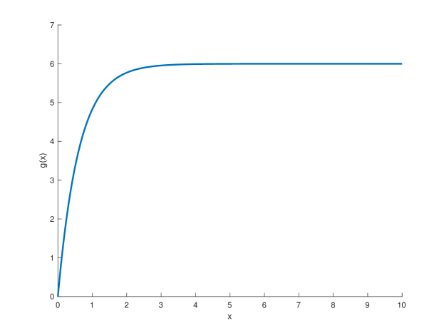
Figure 1: The function $g(x)$ when $\mu=0.4$, $r=0.05$, $\sigma=0.4$, $\overline{c}=0.3$

Before giving the HJB equation, we first study a simple case, for which we can give an explicit optimal dividend ratcheting strategy and the optimal value.

2.2 The Simple Case: $2\mu\overline{c}\leq\sigma^{2}r.$

Theorem 2.2

Suppose $2\mu\overline{c}\leq\sigma^{2}r$. Then $V(x,c)=g(x)$ for all $(x,c)\in{\cal Q}$ and $\mathcal{C}^{*}_{t}\equiv\overline{c}$ is an optimal dividend ratcheting strategy to the problem (3).

To prove this theorem, we need the following technical result.

Lemma 2.3

The inequality $\overline{c}\gamma\leq r$ holds if and only if $2\mu\overline{c}\leq\sigma^{2}r$.

Proof: Note that the function $f(y)=-\frac{1}{2}\sigma^{2}y^{2}+(\mu-\overline{c})y+r$ satisfies $f(y)>0$ if $y\in(0,\gamma)$ and $f(y)\leq 0$ if $y\geq\gamma$, so $\gamma\leq r/\overline{c}$ is equivalent to $f(r/\overline{c})\leq 0$, i.e. $2\mu\overline{c}\leq\sigma^{2}r$. $\Box$

Proof of Theorem 2.2: If $2\mu\overline{c}\leq\sigma^{2}r$, then by Lemma 2.3,

$$g^{\prime}(x)=\frac{\overline{c}\gamma}{r}e^{-\gamma x}\leq 1,~{}x\in{\mathbb{R}}^{+}.$$

This together with (6) yields

$$-{\cal L}_{c}g-c=-{\cal L}_{c}g-c-(-{\cal L}_{\overline{c}}g-\overline{c})=(c-\overline{c})(g^{\prime}-1)\geq 0,~{}x\in{\mathbb{R}}^{+}.$$

Therefore, for any constant $T>0$ and admissible strategy $\{\mathcal{C}_{t}\}_{t\geq 0}\in\Pi_{[c,\overline{c}]}$, applying Itô’s formula to $e^{-rt}g(X_{t})$ on $[0,\tau\wedge T]$ gives

$$g(x) ={\mathbb{E}}[e^{-r(\tau\wedge T)}g(X_{\tau\wedge T})]-{\mathbb{E}}\Bigg{[}\int_{0}^{\tau\wedge T}e^{-rt}{\cal L}_{\mathcal{C}_{t}}g(X_{t})\>{\rm d}t\Bigg{]}-{\mathbb{E}}\Bigg{[}\int_{0}^{\tau\wedge T}e^{-rt}\sigma g^{\prime}(X_{t})\>{\rm d}W_{t}\Bigg{]}$$

$$\geq{\mathbb{E}}\Bigg{[}\int_{0}^{\tau\wedge T}e^{-rt}\ \mathcal{C}_{t}\>{\rm d}t\Bigg{]},$$

where we used the fact that $g\geq 0$ and $g^{\prime}$ is bounded to get the inequality. Sending $T\to\infty$ in above, we get from the monotone convergence theorem that

$$g(x) \geq{\mathbb{E}}\Bigg{[}\int_{0}^{\tau}e^{-rt}\ \mathcal{C}_{t}\>{\rm d}t\Bigg{]}.$$

Since $\{\mathcal{C}_{t}\}_{t\geq 0}\in\Pi_{[c,\overline{c}]}$ is arbitrary selected, the above shows that $g\geq V$ on ${\cal Q}$.

Furthermore, under the special dividend ratcheting strategy $\mathcal{C}^{*}_{t}\equiv\overline{c}$, which is clearly admissible, one can show similarly to the boundary case that

$$g(x) ={\mathbb{E}}\Bigg{[}\int_{0}^{\tau}e^{-rt}\ \mathcal{C}^{*}_{t}\>{\rm d}t\Bigg{]}.$$

This together with $g\geq V$ on ${\cal Q}$ shows that $\mathcal{C}^{*}_{t}\equiv\overline{c}$ is an optimal dividend ratcheting strategy to the problem (3) and $V=g$ on ${\cal Q}$. $\Box$

From this result we can see that if the maximum dividend payout rate is relatively small (i.e. $\overline{c}\leq\sigma^{2}r/\mu)$, then it is optimal for the insurance company to pay dividends to the shareholders at the maximum rate all the time, regardless its surplus level. Intuitively speaking, a higher dividend payout rate benefits the utility more than its negative impact on the survival time. We can also interpret the result from another point of view. If the income process has a relatively high risk/uncertainty (i.e. $2\mu\overline{c}/r\leq\sigma^{2}$), then it is optimal to pay dividends at the maximum rate. Intuitively speaking, because of the highly uncertainty of the income process, the insurance company has a higher risk to be bankrupt in the near future, so it is better to pay dividends as soon as possible.

In the rest of the paper, we deal with the much more complicated case: $2\mu\overline{c}>\sigma^{2}r$, which is assumed from now on. Note the condition $2\mu\overline{c}>\sigma^{2}r$ by Lemma 2.3 is equivalent to that $g^{\prime}(0)>1$.

3 The HJB equation and optimal dividend ratcheting strategy in the complicated case $2\mu\overline{c}>\sigma^{2}r$

The HJB equation for the optimization problem (3) is a variational inequality on $v:{\cal Q}\to{\mathbb{R}}$:

$$\begin{cases}\min\big{\{}\!-{\cal L}_{c}v-c,~{}-v_{c}\big{\}}=0,&(x,c)\in{\cal Q},\vskip 12.0pt plus 4.0pt minus 4.0pt\\ v(0,c)=0,&c\in[0,\overline{c}],\vskip 12.0pt plus 4.0pt minus 4.0pt\\ v(x,\overline{c})=g(x),&x\in{\mathbb{R}}^{+},\end{cases}$$ (8)

where the function $g$ is defined in (5), and the operator ${\cal L}_{c}$ is defined in (7). Thanks to the estimate (4), it suffices to study bounded solution(s) to the above HJB equation (8). Note that $v=g$ is a solution to (8) if $2\mu\overline{c}\leq\sigma^{2}r$, and not a solution otherwise.

It is proved in [Albrecher et al., 2020] that the problem (8) admits a unique viscosity solution, which is the value function $V$ defined in (3). In this paper, we will further prove that (8) admits a solution in the following stronger sense. Unlike [Albrecher et al., 2020], our solution will allow us to construct an optimal dividend ratcheting strategy for the problem (3), thus solve the problem completely.

Definition 3.1

We call a function $v:{\cal Q}\to{\mathbb{R}}$ is a solution to the problem (8) if

1. it holds that $v\in{\cal A}$, where

   $${\cal A}=\Big{\{}v:{\cal Q}\to{\mathbb{R}}\;\Big{|}\; v v_{x} v_{c} {\cal Q} v_{c}\leq 0 {\cal Q}$$ , and are continuous and bounded in ; in ;

   $$\mbox{and $v(\cdot,c)\in W^{2,\>p}_{\rm loc}({\mathbb{R}}^{+})$ for each $c\in[0,\overline{c}]$ and $p>1$}\Big{\}};$$

2. it satisfies the boundary conditions in (8);

3. it holds that

   $$-{\cal L}_{c}v(\cdot,c)-c\geq 0\hbox{\; a.e.\;in ${\mathbb{R}}^{+}$, for each $c\in[0,\overline{c}]$};$$ (9)

4. if $v_{c}(x,c)<0$ for some $(x,c)\in{\cal Q}$, then

   $$-{\cal L}_{c}v(y,c)-c=0\hbox{\; for all $y\in[0,x]$}.$$ (10)

As usual, the notation $W^{2,\>p}_{\rm loc}$ stands for the Sobolev space. We remark that the last requirement (10) is in the classical sense rather than the strong sense.

In the variational inequality in (8), the obstacle is put on $v_{c}$, but the equation is for $v$, so it is natural to transform the problem (8) into one for $u=-v_{c}$. Since $v(x,\overline{c})=g(x)$, we shall have

$$v(x,c)=g(x)+\int_{c}^{\overline{c}}u(x,s)\>{\rm d}s.$$

It then implies

$${\partial}_{c}(-{\cal L}_{c}v-c)={\cal L}_{c}(-v_{c})+v_{x}-1={\cal L}_{c}u+g^{\prime}(x)+\int_{c}^{\overline{c}}u_{x}(x,s)\>{\rm d}s-1,$$

so we conjecture an obstacle problem for $u$:

$$\begin{cases}\displaystyle\min\bigg{\{}\!-{\cal L}_{c}u-g^{\prime}(x)-\int_{c}^{\overline{c}}u_{x}(x,s)\>{\rm d}s+1,~{}u\bigg{\}}=0,&(x,c)\in{\cal Q},\vskip 12.0pt plus 4.0pt minus 4.0pt\\ u(0,c)=0,&c\in[0,\overline{c}].\end{cases}$$ (11)

This is a single-obstacle problem with nonlocal operator.

Definition 3.2

We call a function $u:{\cal Q}\to{\mathbb{R}}$ is a solution to the problem (11) if

1. it holds that $u\in{\cal B}$, where

   $${\cal B}=\Big{\{}u:{\cal Q}\to{\mathbb{R}}^{+}\;\Big{|}\; u u_{x} {\cal Q}$$ and are continuous and bounded in ;

   $$\mbox{and $u(\cdot,c)\in W^{2,\>p}_{\rm loc}({\mathbb{R}}^{+})$ for each $c\in[0,\overline{c}]$ and $p>1$}\Big{\}};$$

2. for each $c\in[0,\overline{c}]$, it holds that

   $$-{\cal L}_{c}u-g^{\prime}(x)-\int_{c}^{\overline{c}}u_{x}(x,s)\>{\rm d}s+1\geq 0\hbox{\; a.e.\;in ${\mathbb{R}}^{+}$};$$ (12)

3. if $u(x,c)>0$ for some $(x,c)\in{\cal Q}$, then it holds that

   $$-{\cal L}_{c}u(y,c)-g^{\prime}(y)-\int_{c}^{\overline{c}}u_{x}(y,s)\>{\rm d}s+1=0\hbox{\; for all $y\in[0,x]$}.$$ (13)

Combining (8) and (11), we obtain a system of variational inequalities on $(v,u)$:

$$\begin{cases}\min\big{\{}\!-{\cal L}_{c}v-c,~{}u\big{\}}=0,&(x,c)\in{\cal Q},\vskip 12.0pt plus 4.0pt minus 4.0pt\\ \min\big{\{}\!-{\cal L}_{c}u+v_{x}-1,~{}u\big{\}}=0,&(x,c)\in{\cal Q},\vskip 12.0pt plus 4.0pt minus 4.0pt\\ v(0,c)=0,~{}u(0,c)=0,&c\in[0,\overline{c}],\vskip 12.0pt plus 4.0pt minus 4.0pt\\ v(x,\overline{c})=g(x),&x\in{\mathbb{R}}^{+},\end{cases}$$ (14)

Our next main result concerns the solvability of (8), (11) and (14).

Theorem 3.3

There exists a pair $(v,u)$ that satisfies (14) and

$$v(x,c)=g(x)+\int_{c}^{\overline{c}}u(x,s)\>{\rm d}s,~{}(x,c)\in{\cal Q}.$$ (15)

Also, $v$ and $u$ are, respectively, solutions to (8) and (11) in the sense of Definition 3.1 and Definition 3.2. Furthermore, for each $\alpha\in(0,1)$, there exists a constant $K>0$ such that, for all $(x,c)\in{\cal Q}$,

$$0\leq v\leq\frac{\overline{c}}{r},$$ (16)

$$0\leq v_{x}\leq K,$$ (17)

$$0\leq-v_{c}\leq K,$$ (18)

and

$$v_{x}(y,c)\leq\max\{v_{x}(x,c),1\},~{}\forall\;0\leq x\leq y,$$ (19)

$$|u(\cdot,c)|_{C^{1+\alpha}({\mathbb{R}}^{+})}\leq K,$$ (20)

$$|u_{c}(\cdot,c)|\leq K.$$ (21)

This result will be proved in Section 4.2.

From (19), we see that the whole space ${\cal Q}$ can be divided into two regions $\{v_{x}>1\}$ and $\{v_{x}\leq 1\}$ by a surface. See Figure 2 for an illustration.

Figure 2: The two regions $\{v_{x}>1\}$ and $\{v_{x}\leq 1\}$.

We can also see from (19) that $x\to v_{x}(x,c)$ is a concave function in the region $\{v_{x}>1\}$. Indeed, numerical examples show that it is concave for all $x\in{\mathbb{R}}^{+}$; see Figure 3. However, we cannot prove this.

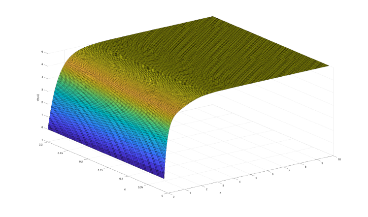
Figure 3: The value function $v$ where $\mu=0.4$, $r=0.05$, $\sigma=0.4$, $\overline{c}=0.3$.

The following result fully characterizes the free boundary, which is crucial to determine the optimal dividend ratcheting strategy.

Theorem 3.4

Let $v$ be a solution to (8) given in Theorem 3.3. Define the dividend ratcheting free boundary:

$$\mathcal{X}(c)=\inf\big{\{}x>0\;\big{|}\;v_{c}(x,c)=0\big{\}},~{}c\in[0,\overline{c}].$$

Then $\mathcal{X}(c)>0$ for all $c\in[0,\overline{c}].$ Also,

1. It holds for all $c\in[0,\overline{c}]$ that $v_{c}(x,c)=0$ if $x\geq\mathcal{X}(c)$ and $v_{c}(x,c)<0$ if $x<\mathcal{X}(c)$.

2. It holds that $\mathcal{X}(\cdot)\in C^{\infty}[0,\overline{c}].$

3. There exit two constants $0<K_{1}<K_{2}$ such that $K_{1}\leq\mathcal{X}^{\prime}(c)\leq K_{2}$ for all $c\in[0,\overline{c}]$. As a consequence, both $\mathcal{X}(\cdot)$ and its inverse $\mathcal{X}^{-1}(\cdot)$ are strictly increasing and Lipschitz continuous.

Figure 4 illustrates the dividend ratcheting free boundary $\mathcal{X}(\cdot)$. Above the free boundary, we have $v_{c}=0$, which means it will not change the optimal value if one ratchet up the dividend payout rate up to the boundary. In other words, the function $v$ takes a constant value on each horizon line on the left of the free boundary (where $v_{c}=0$). In particular, we have $v(x,c)=v(x,\overline{c})=g(x)$ if $x\geq\mathcal{X}(\overline{c})$. By contrast, the function $v$ is strictly decreasing on each horizon line on the right of the free boundary (where $v_{c}<0$), therefore, one should not ratchet up the dividend payout rate below the free boundary since it will reduce the optimal value.

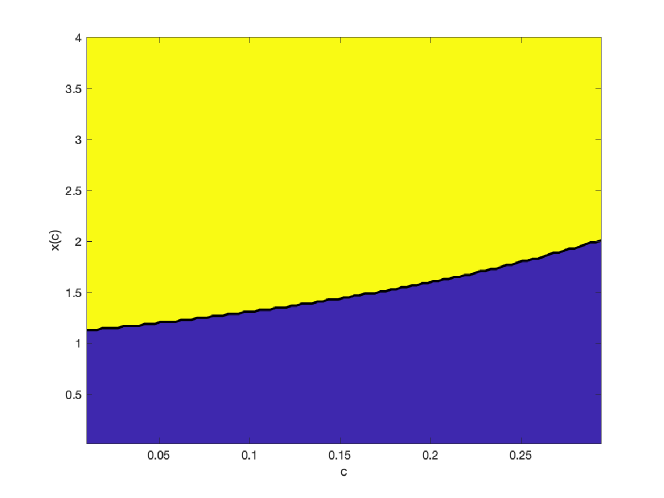
Figure 4: The free boundary $\mathcal{X}(\cdot)$ where $\mu=0.4$, $r=0.05$, $\sigma=0.4$, $\overline{c}=0.3$.

The above properties 1, 2 and 3 will be proved respectively in Lemma 5.4, Proposition 5.1 and Proposition 5.2. These properties will be used to construct an optimal dividend ratcheting strategy to the problem (3) in the complicated case $2\mu\overline{c}>\sigma^{2}r$ in the next section.

3.1 Optimal Dividend Ratcheting Strategy

Since $\mathcal{X}(\cdot)$, given in Theorem 3.4, is strictly increasing, we may define

$$\mathfrak{C}_{[c,\overline{c}]}(x)=\begin{cases}c,&0\leq x\leq\mathcal{X}(c);\\ \mathcal{X}^{-1}(x),&\mathcal{X}(c)<x<\mathcal{X}(\overline{c});\\ \overline{c},&x\geq\mathcal{X}(\overline{c}).\end{cases}$$ (22)

By Theorem 3.4, the function $\mathfrak{C}_{[c,\overline{c}]}(\cdot)$ is Lipschitz continuous, bounded and non-decreasing on ${\mathbb{R}}^{+}$. Also, by the definition (22),

$$\mathcal{X}\big{(}\mathfrak{C}_{[c,\overline{c}]}(x)\big{)}=\max\big{\{}\mathcal{X}(c),~{}x\big{\}}\hbox{\; if $\mathfrak{C}_{[c,\overline{c}]}(x)<\overline{c}$.}$$ (23)

We are now ready to provide a complete answer to the problem (3).

Theorem 3.5

Let $v$ be a solution to (8) given in Theorem 3.3. Then it is the optimal value of the optimal dividend ratcheting problem (3). Moreover, $\{\mathcal{C}^{*}_{t}\}_{t\geq 0}$ is an optimal dividend ratcheting strategy to the problem (3), where

$$\mathcal{C}^{*}_{t}=\mathfrak{C}_{[c,\overline{c}]}\Big{(}\max\limits_{p\in[0,t]}X^{*}_{p}\Big{)},$$

and $\mathfrak{C}_{[c,\overline{c}]}(\cdot)$ is defined in (22), and $X^{*}_{t}$ is the unique strong solution to the following SDE:

$$X^{*}_{t}=x+\int_{0}^{t}\Big{(}\mu-\mathfrak{C}_{[c,\overline{c}]}\big{(}\max\limits_{p\in[0,s]}X^{*}_{p}\big{)}\Big{)}\>{\rm d}s+\sigma W_{t}.$$ (24)

Proof: Suppose $V(x,c)$ is the value function defined in (3) and $v(x,c)$ is the solution to the problem (8) given in Theorem 3.3. We come to prove $v(x,c)=V(x,c)$ for any $(x,c)\in{\cal Q}$.

For any admissible dividend ratcheting strategy $\{\mathcal{C}_{t}\}_{t\geq 0}\in\Pi_{[c,\overline{c}]}$, let $X_{t}$ be the corresponding solution to (1) with the initial value $X_{0}=x$. Let $T>0$ be any constant. Then Itô’s formula gives

$$v(x,c) ={\mathbb{E}}[e^{-r(\tau\wedge T)}v(X_{\tau\wedge T},\mathcal{C}_{\tau\wedge T})]-{\mathbb{E}}\Bigg{[}\int_{0}^{\tau\wedge T}e^{-rt}{\cal L}_{\mathcal{C}_{t}}v(X_{t},\mathcal{C}_{t})\>{\rm d}t\Bigg{]}$$

$$\quad\;-{\mathbb{E}}\Bigg{[}\int_{0}^{\tau\wedge T}e^{-rt}v_{c}(X_{t},\mathcal{C}_{t})\>{\rm d}\mathcal{C}_{t}\Bigg{]}-{\mathbb{E}}\Bigg{[}\int_{0}^{\tau\wedge T}e^{-rt}\sigma v_{x}(X_{t},\mathcal{C}_{t})\>{\rm d}W_{t}\Bigg{]}.$$

Thanks to the boundedness of $v_{x}$, the last expectation is zero. Since $-{\cal L}_{\mathcal{C}_{t}}v(X_{t},\mathcal{C}_{t})-\mathcal{C}_{t}\geq 0$, $-v_{c}(X_{t},\mathcal{C}_{t})\geq 0$ and $\>{\rm d}\mathcal{C}_{t}\geq 0$, we have

$$v(x,c)\geq{\mathbb{E}}[e^{-r(\tau\wedge T)}v(X_{\tau\wedge T},\mathcal{C}_{\tau\wedge T})]+{\mathbb{E}}\Bigg{[}\int_{0}^{\tau\wedge T}e^{-rt}\mathcal{C}_{t}\>{\rm d}t\Bigg{]}.$$ (25)

Since $v\geq 0$, the first expectation can be dropped, giving

$$v(x,c)\geq{\mathbb{E}}\Bigg{[}\int_{0}^{\tau\wedge T}e^{-rt}\mathcal{C}_{t}\>{\rm d}t\Bigg{]}.$$

Since $\mathcal{C}_{t}$ is nonnegative, applying the monotone convergence theorem to above leads to

$$v(x,c)\geq{\mathbb{E}}\Bigg{[}\int_{0}^{\tau}e^{-rt}\mathcal{C}_{t}\>{\rm d}t\Bigg{]}.$$

Since $\{\mathcal{C}_{t}\}_{t\geq 0}\in\Pi_{[c,\overline{c}]}$ is arbitrary selected, we obtain $v(x,c)\geq V(x,c)$.

Because $\mathfrak{C}_{[c,\overline{c}]}(\cdot)$ is Lipschitz continuous and bounded, by [Mao, 2008, Theorem 2.2, p.150], there exists a unique strong solution $X^{*}_{t}$ to the SDE (24). Set

$$\mathcal{C}^{*}_{t}=\mathfrak{C}_{[c,\overline{c}]}\Big{(}\max\limits_{p\in[0,t]}X^{*}_{p}\Big{)}.$$

Then it is not hard to check that $\{\mathcal{C}^{*}_{t}\}_{t\geq 0}$ is an admissible dividend ratcheting strategy in $\Pi_{[c,\overline{c}]}$. Clearly, $X^{*}_{t}$ is the corresponding solution to (1) under the strategy $\{\mathcal{C}^{*}_{t}\}_{t\geq 0}$ with the initial value $X_{0}=x$. We now prove that $\{\mathcal{C}^{*}_{t}\}_{t\geq 0}$ is an optimal dividend ratcheting strategy to the problem (3) and $v(x,c)=V(x,c)$.

We first prove

$$-{\cal L}_{\mathcal{C}^{*}_{t}}v(X^{*}_{t},\mathcal{C}^{*}_{t})-\mathcal{C}^{*}_{t}=0.$$ (26)

In fact, if $\mathcal{C}^{*}_{t}=\overline{c}$, then (26) holds true since

$$-{\cal L}_{\overline{c}}v(x,\overline{c})-\overline{c}=-{\cal L}_{\overline{c}}g(x)-\overline{c}=0,~{}x\in{\mathbb{R}}^{+}.$$

Now suppose $\mathcal{C}^{*}_{t}<\overline{c}$. Then by (23),

$$\mathcal{X}(\mathcal{C}^{*}_{t})=\max\Big{\{}\mathcal{X}(c),~{}\max\limits_{p\in[0,t]}X^{*}_{p}\Big{\}},$$

so

$$X^{*}_{t}\leq\mathcal{X}(\mathcal{C}^{*}_{t}).$$

It thus follows from Theorem 3.4 and (10) that (26) holds.

On the other hand, we have $\>{\rm d}\mathcal{C}^{*}_{t}=0$ if $X^{*}_{t}\neq\mathcal{X}(\mathcal{C}^{*}_{t})$, and thanks to Theorem 3.4, $v_{c}(X^{*}_{t},\mathcal{C}^{*}_{t})=0$ if $X^{*}_{t}=\mathcal{X}(\mathcal{C}^{*}_{t})$, so it always holds that

$$-v_{c}(X^{*}_{t},\mathcal{C}^{*}_{t})\>{\rm d}\mathcal{C}^{*}_{t}=0,~{}0\leq t\leq\tau.$$

Therefore, under the strategy $\{\mathcal{C}^{*}_{t}\}_{t\geq 0}$, the inequality (25) becomes an equation

$$v(x,c)={\mathbb{E}}[e^{-r(\tau\wedge T)}v(X^{*}_{\tau\wedge T},\mathcal{C}^{*}_{\tau\wedge T})]+{\mathbb{E}}\Bigg{[}\int_{0}^{\tau\wedge T}e^{-rt}\mathcal{C}^{*}_{t}\>{\rm d}t\Bigg{]}.$$ (27)

If $\tau<\infty$, then $X^{*}_{\tau}=0$ and hence,

$$\lim_{T\to\infty}e^{-r(\tau\wedge T)}v(X^{*}_{\tau\wedge T},\mathcal{C}^{*}_{\tau\wedge T})=e^{-r\tau}v(X^{*}_{\tau},\mathcal{C}^{*}_{\tau})=e^{-r\tau}v(0,\mathcal{C}^{*}_{\tau})=0.$$

If $\tau=\infty$, then, since $v$ is bounded and $r>0$,

$$\lim_{T\to\infty}e^{-r(\tau\wedge T)}v(X^{*}_{\tau\wedge T},\mathcal{C}^{*}_{\tau\wedge T})=\lim_{T\to\infty}e^{-rT}v(X^{*}_{T},\mathcal{C}^{*}_{T})=0.$$

Now applying the dominated convergence theorem to the first integral and the monotone convergence theorem to the second integral in (27), we get

$$v(x,c)={\mathbb{E}}\Bigg{[}\int_{0}^{\tau}e^{-rt}\mathcal{C}^{*}_{t}\>{\rm d}t\Bigg{]}.$$

In view of the definition of $V(x,c)$, we obtain $v(x,c)\leq V(x,c)$. Therefore, $v(x,c)=V(x,c)$, and $\{\mathcal{C}^{*}_{t}\}_{t\geq 0}$ is an optimal dividend ratcheting strategy. $\Box$

Different from the simple case, we can see from this result that, in the complicated case, the optimal dividend ratcheting strategy relays on the surplus level and one should only ratchet up the dividend payout rate when the surplus level touches the dividend ratcheting free boundary.

The reminder of the paper is devoted to establishing Theorems 3.3 and 3.4 by a novel PDE method.

4 Solvability of the HJB Equations (8) and (11)

This section consists of two parts. In the first part, we introduce and study a regime switching system to approximate the HJB equations (8) and (11). In the second part, we construct a solution to (8) and (11) by a limit argument.

We will use the following technical result frequently in our subsequent analysis.

Lemma 4.1

Suppose $a\geq 0$ is a constant, and $h:[a,\infty)\to{\mathbb{R}}^{+}$ is a given bounded measurable function. If $\nu\in W^{2,\>p}_{\rm loc}[a,\infty)\cap L^{\infty}([a,\infty))$ for some $p>1$ and satisfies

$$\begin{cases}\min\big{\{}\!-{\cal L}_{c}\nu+h,~{}\nu\big{\}}=0,&x>a,\vskip 12.0pt plus 4.0pt minus 4.0pt\\ \nu(a)=0\end{cases}$$ (28)

for some $c\in[0,\overline{c}]$. Then $\nu\equiv 0$ in $[a,\infty)$.

Proof: It is easy to check that $\nu(x)\equiv 0$, $x\geq a$ satisfies (28), by the uniqueness of the solution of (28) in $\nu\in W^{2,\>p}_{\rm loc}[a,\infty)\cap L^{\infty}([a,\infty))$, we get the conclusion. $\Box$

4.1 A Regime Switching Approximation System

Suppose $n\geq 1$ and the dividend payout rates can only take the following finite values

$$c_{i}=\overline{c}-i\Delta c,~{}i=0,1,2,\cdots,n,$$

with $\Delta c=\overline{c}/n>0$. Let $v_{-1}=-1$. We consider the following regime switching ODE system:

$$\begin{cases}\min\big{\{}\!-{\cal L}_{c_{i}}v_{i}-c_{i},~{}v_{i}-v_{i-1}\big{\}}=0,&x>0,\vskip 12.0pt plus 4.0pt minus 4.0pt\\ v_{i}(0)=0,&i=0,1,2,\cdots,n,\end{cases}$$ (29)

under the power growth condition. Here, we can think of $v_{i}(x)$ as an approximation of $v(x,c_{i})$. This is a system of single-obstacle problems, so we can solve it.

Lemma 4.2

The system (29) admits a unique solution $v_{i}\in W^{2,\>p}_{\rm loc}({\mathbb{R}}^{+})\cap C^{1+\alpha}({\mathbb{R}}^{+})$, $i=0,1,2,\cdots,n,$ for any $p>1$ and $\alpha\in(0,1)$. Moreover, it holds that

$$0\leq v_{i}\leq\frac{\overline{c}}{r},$$ (30)

$$v_{i}^{\prime}\geq 0$$ (31)

and

$$v_{i}^{\prime}(y)\leq\max\big{\{}v_{i}^{\prime}(x),~{}1\big{\}},~{}\forall\;0\leq x\leq y.$$ (32)

Let

$$x_{i}=\inf\big{\{}x>0\;|\;v_{i}(x)=v_{i-1}(x)\big{\}},~{}i=0,1,2,\cdots,n,$$ (33)

then $v_{i}(x)=v_{i-1}(x)$ if $x\geq x_{i}$ and $v_{i}(x)>v_{i-1}(x)$ if $x<x_{i}$. Also, $0<x_{i}<\infty$ for $i=1,2,\cdots,n,$ and $x_{0}=+\infty$.

Proof: Because $g\geq 0>v_{-1}$ and $c_{0}=\overline{c}$, it follows from (6) that

$$\begin{cases}\min\big{\{}\!-{\cal L}_{c_{0}}g-c_{0},~{}g-v_{-1}\big{\}}=-{\cal L}_{\overline{c}}g-\overline{c}=0,&x>0,\\ g(0)=0.&\end{cases}$$

Therefore, $v_{0}=g$ is the unique solution to (29) in $W^{2,\>p}_{\rm loc}({\mathbb{R}}^{+})\cap C^{1+\alpha}({\mathbb{R}}^{+})$ and $x_{i}=+\infty$ when $i=0$.

For each $i=1,2,\ldots,n$, the problem (29) is a single-obstacle problem. By the standard penalty method and $L^{p}$ theorem, we can prove step by step for $i$ from $1$ to $n$ that (29) admits a unique solution (See, e.g., [Friedman, 1975]):

$$v_{i}\in W^{2,\>p}_{\rm loc}({\mathbb{R}}^{+}).$$

Moreover, by the embedding theorem (See, e.g., [Evans, 2017, Theorem 6 on page 286]), we also have

$$v_{i}\in C^{1+\alpha}({\mathbb{R}}^{+}).$$

Since the process is standard, we omit the details.

By (29),

$$v_{i}\geq v_{i-1}\geq\cdots\geq v_{0}\geq 0>v_{-1},$$ (34)

giving the lower bound in (30).

We now prove the remaining claims by mathematical induction. It is easy to check that $v_{0}=g$ satisfies all the desired properties. Suppose all the desired results of the lemma hold for $i=j-1$ ($1\leq j<n$), we now prove that they also hold when $i=j$.

Because $v_{j-1}\leq\overline{c}/r$, the constant function $\overline{c}/r$ is a super solution to the variational inequality of $v_{j}$ by (29). Hence we proved the upper bound in (30): $v_{j}\leq\overline{c}/r$.

We now prove the set

$$E_{j}:=\{x>0\;|\;v_{j}(x)=v_{j-1}(x)\}$$

is not empty. Suppose, on the contrary, it is empty. Then by the variational inequality (29), we have

$$-{\cal L}_{c_{j}}v_{j}-c_{j}=0,~{}x>0.$$

It admits an explicit solution

$$v_{j}(x)=\frac{c_{j}}{r}(1-e^{-\gamma_{j}x}),$$

under the initial condition $v_{j}(0)=0$ and power growth condition, where $\gamma_{j}$ is the positive root of

$$-\frac{1}{2}\sigma^{2}\gamma_{j}^{2}+(\mu-c_{j})\gamma_{j}+r=0.$$

It hence follows

$$v_{j}(+\infty)=c_{j}/r<\overline{c}/r=v_{0}(+\infty),$$

contradicting to the order (34). Therefore, $E_{j}$ is not empty. As a consequence, we have

$$x_{j}:=\inf E_{j}<\infty.$$

We next prove

$$v_{j-1}^{\prime}(x)\leq 1,~{}x\geq x_{j}.$$ (35)

Thanks to (32), it suffices to prove $v_{j-1}^{\prime}(x^{*})\leq 1$ for all $x^{*}\in E_{j}$. Suppose, on the contrary, $v_{j-1}^{\prime}(x^{*})>1$ for some $x^{*}\in E_{j}$. Then by the order (34), there must exist $1\leq k\leq j$ such that

$$v_{j}(x^{*})=v_{j-1}(x^{*})=\cdots=v_{j-k}(x^{*})>v_{j-k-1}(x^{*}).$$

Since $v_{j-k}$ and $v_{j-k-1}$ are continuous, there exists a neighborhood $I_{\varepsilon}=[x^{*}-\varepsilon,x^{*}+\varepsilon]$ such that $v_{j-k}>v_{j-k-1}$ in $I_{\varepsilon}$, so by (29),

$$-{\cal L}_{c_{j-k}}v_{j-k}-c_{j-k}=0\quad\hbox{in }I_{\varepsilon}.$$

Together with the variational inequality of $v_{j}$, we obtain the estimate

$$\frac{\sigma^{2}}{2}(v_{j}-v_{j-k})^{\prime\prime}\leq-(\mu-c_{j})(v_{j}^{\prime}-v_{j-k}^{\prime})+r(v_{j}-v_{j-k})+k\Delta c(1-v_{j-k}^{\prime})\quad\hbox{ a.e. in }I_{\varepsilon}.$$ (36)

Note that both $v_{j}-v_{j-1}$ and $v_{j}-v_{j-k}$ attain their minimum value $0$ at $x^{*}$, so

$$v_{j}(x^{*})=v_{j-1}(x^{*})=v_{j-k}(x^{*}),~{}v_{j}^{\prime}(x^{*})=v_{j-1}^{\prime}(x^{*})=v_{j-k}^{\prime}(x^{*})>1.$$

which shows that the right hand side (RHS) of (36) is negative at $x^{*}$. Because the RHS of (36) is continuous, we conclude that $(v_{j}-v_{j-k})^{\prime\prime}<0$ a.e. in $I_{\varepsilon}$ when $\varepsilon>0$ is small enough. This means $v_{j}-v_{j-k}$ is strictly concave in $I_{\varepsilon}$, which contradicts that $v_{j}-v_{j-k}$ attains its minimum value at the inner point $x^{*}\in I_{\varepsilon}$. Thus, we established (35).

We next prove

$$v_{j}(x)=v_{j-1}(x),~{}x\geq x_{j}.$$ (37)

Let $\nu=v_{j}-v_{j-1}$. Then, by (29),

$$\begin{cases}\min\big{\{}\!-{\cal L}_{c_{j}}\nu-{\cal L}_{c_{j}}v_{j-1}-c_{j},~{}\nu\big{\}}=\min\big{\{}\!-{\cal L}_{c_{j}}v_{j}-c_{j},~{}v_{j}-v_{j-1}\big{\}}=0,&x>x_{j},\vskip 12.0pt plus 4.0pt minus 4.0pt\\ \nu(x_{j})=v_{j}(x_{j})-v_{j-1}(x_{j})=0.\end{cases}$$

Note (29) also holds when $i=j-1$ by the inductive hypothesis. Together with (35), we get

$$-{\cal L}_{c_{j}}v_{j-1}(x)-c_{j}=-{\cal L}_{c_{j-1}}v_{j-1}(x)-c_{j-1}+\Delta c(1-v_{j-1}^{\prime}(x))\geq 0,~{}x>x_{j},$$

Applying Lemma 4.1, we conclude $\nu=0$ for $x>x_{j}$ so that (37) holds. As a consequence, $x_{j}$ is the unique free boundary point such that $v_{j}(x)=v_{j-1}(x)$ if $x\geq x_{j}$ and $v_{j}(x)>v_{j-1}(x)$ if $x<x_{j}$.

Note that $v_{j}\geq g$, $v_{j}(0)=g(0)=0$ and $g^{\prime}(0)>1$ in the complicated case, so

$$v_{j}^{\prime}(0)\geq g^{\prime}(0)>1,$$ (38)

which together with (35) gives

$$x_{j}>0.$$ (39)

We come to prove $v_{j}^{\prime}\geq 0$. Since $v_{j}=v_{j-1}$ in $[x_{j},+\infty)$ by (37) and $v_{j-1}^{\prime}\geq 0$ by the inductive hypothesis, we only need to prove

$$v_{j}^{\prime}\geq 0\quad\hbox{in}\;[0,x_{j}).$$ (40)

Differentiating the equation in (29) we have

$$-{\cal L}_{c_{j}}(v_{j}^{\prime})=0\quad\hbox{in}\;(0,x_{j}).$$ (41)

Notice (38) and $v_{j}^{\prime}(x_{j})=v_{j-1}^{\prime}(x_{j})\geq 0$ by (37), we conclude from the maximum principle that (40) holds.

Finally, fix any $x\in{\mathbb{R}}^{+}$. We now prove, for all $y\geq x$,

$$v_{j}^{\prime}(y)\leq\max\big{\{}v_{j}^{\prime}(x),~{}1\big{\}}.$$ (42)

Combining (35) and (37), we know (42) is true for $y\in[x_{j},+\infty)$. Applying (35), it is easy to check that the constant function $\max\big{\{}v_{j}^{\prime}(x),~{}1\big{\}}$ is a super solution to (41) in $[x,x_{j}]$, so (42) holds for $y\in[x,x_{j}]$ as well. The proof is complete. $\Box$
In the rest of this paper, we keep the notations $v_{i}$ and $x_{i}$ given in Lemma 4.2.

We next prove that the inequality (35) holds strictly at $x=x_{j}$.

Lemma 4.3

For each $j=1,2,\cdots,n$, we have

$$v_{j-1}^{\prime}(x_{j})<1.$$ (43)

Proof: Suppose, on the contrary, suppose $v_{j-1}^{\prime}(x_{j})=1$. Same as before, there must exist $1\leq k\leq j$ such that

$$v_{j}(x_{j})=v_{j-1}(x_{j})=\cdots=v_{j-k}(x_{j})>v_{j-k-1}(x_{j}).$$

By continuity, $v_{j-k}>v_{j-k-1}$ near $x_{j}$, so $-{\cal L}_{c_{j-k}}v_{j-k}-c_{j-k}=0$ by (29), which confirms the continuity of $v_{j-k}^{\prime\prime}$ near $x_{j}$. Note that both $v_{j}-v_{j-1}$ and $v_{j}-v_{j-k}$ attain their minimum value $0$ at $x_{j}$, so

$$v_{j}^{\prime}(x_{j})=v_{j-1}^{\prime}(x_{j})=v_{j-k}^{\prime}(x_{j})=1.$$ (44)

Together with (32) we obtain $v_{j-k}^{\prime\prime}(x_{j})\leq 0$. Moreover, it follows from (38) and (32) that $v_{j-k}^{\prime}(x)\leq v_{j-k}^{\prime}(0)$ for all $x\geq 0$; and consequently, $v_{j-k}^{\prime\prime}(0)\leq 0$. Differentiating the equation of $v_{j-k}$ in $[0,x_{j}]$ twice we obtain

$$-{\cal L}_{c_{j-k}}(v_{j-k}^{\prime\prime})=0.$$

By the maximum principle, we deduce $v_{j-k}^{\prime\prime}\leq 0$ in $[0,x_{j}]$, so $v_{j-k}^{\prime}(x)\geq v_{j-k}^{\prime}(x_{j})=1$ for $x\in[0,x_{j}]$.

Let

$$\psi=v_{j}-v_{j-k}.$$

By the equations of $v_{j}$ and $v_{j-k}$, we see that $\psi$ satisfies

$$-{\cal L}_{c_{j}}\psi=k\Delta c(v_{j-k}^{\prime}-1)\geq 0\quad\hbox{in }[0,x_{j}].$$

Since $\psi$ attains its minimum value 0 at $x_{j}$, we conclude from the Hopf lemma that $\psi^{\prime}(x_{j}-)<0$, but this contradicts (44). The proof is thus complete. $\Box$

The next result establishes the monotonicity of the free boundaries $x_{i}$. To this end, we define

$$u_{i}:=\frac{v_{i}-v_{i-1}}{\Delta c},~{}i=1,2,\cdots,n.$$

in the rest of this paper.

Lemma 4.4

For each $i=1,2,\cdots,n,$ we have

$$\begin{cases}\min\big{\{}\!-{\cal L}_{c_{i}}u_{i}-v_{i-1}^{\prime}+1,~{}u_{i}\big{\}}=0,&x>0.\vskip 12.0pt plus 4.0pt minus 4.0pt\\ u_{i}(0)=0,\end{cases}$$ (45)

Moreover,

$$x_{i}\leq x_{i-1},~{}i=1,2,3,\cdots,n.$$ (46)

Proof: By Lemma 4.2, $x_{i}$ is the number such that $u_{i}(x)>0$ when $x<x_{i}$ and $u_{i}(x)=0$ when $x\geq x_{i}$.

By taking a difference between the equations of $v_{1}$ and $v_{0}$, we know (45) holds when $i=1$. Clearly, (46) holds when $i=1$. Now suppose (45) holds when $i=j-1$ ($2\leq j<n$). We are going to prove $u_{j}$ satisfies (45) and (46) holds when $i=j$.

Suppose $\widehat{u}$ is the unique bounded solution to the variational inequality

$$\begin{cases}\min\big{\{}\!-{\cal L}_{c_{j}}\widehat{u}-v_{j-1}^{\prime}+1,~{}\widehat{u}\big{\}}=0,&x>0,\vskip 12.0pt plus 4.0pt minus 4.0pt\\ \widehat{u}(0)=0,\end{cases}$$ (47)

and let

$$\widehat{x}=\inf\big{\{}x>0\;|\;\widehat{u}(x)=0\big{\}}.$$

It suffices to prove $u_{j}=\widehat{u}$, $x_{j}=\widehat{x}$ and $\widehat{x}\leq x_{j-1}$.

We first prove that

$$v_{j-1}^{\prime}(x)\leq 1\quad\hbox{for all }x\geq\widehat{x}.$$ (48)

By virtue of (32), it suffices to prove $v_{j-1}^{\prime}(x^{*})\leq 1$ for any $x^{*}>0$ such that $\widehat{u}(x^{*})=0$. Suppose, on the contrary, $v_{j-1}^{\prime}(x^{*})>1$. By (47) we have

$$\frac{\sigma^{2}}{2}\widehat{u}^{\prime\prime}\leq-(\mu-c_{j})\widehat{u}^{\prime}+r\widehat{u}-v_{j-1}^{\prime}+1.$$ (49)

Note that $\widehat{u}$ attains its minimum value $0$ at $x^{*}$, so $\widehat{u}(x^{*})=\widehat{u}^{\prime}(x^{*})=0.$ Then the RHS of (49) is continuous and negative at $x^{*}$, so we have $\widehat{u}^{\prime\prime}<0$ in a neighborhood of $x^{*}$. This means that $\widehat{u}$ is strictly concave in that neighborhood, which contradicts that $\widehat{u}$ attains its minimum value at the inner point $x^{*}$ of the neighborhood. Hence, we proved (48).

We next prove that $\widehat{u}>0$ for $x<\widehat{x}$ and $\widehat{u}=0$ for $x\geq\widehat{x}$. By the definition of $\widehat{x}$, it only needs to prove

$$\widehat{u}(x)=0,~{}x\in[\widehat{x},+\infty).$$ (50)

Indeed by (47), we have

$$\begin{cases}\min\big{\{}\!-{\cal L}_{c_{j}}\widehat{u}-v_{j-1}^{\prime}+1,~{}\widehat{u}\big{\}}=0,&x>\widehat{x},\vskip 12.0pt plus 4.0pt minus 4.0pt\\ \widehat{u}(\widehat{x})=0.\end{cases}$$

We thus conclude from (48) and Lemma 4.1 that (50) holds.

Next, we come to prove

$$\widehat{x}\leq x_{j-1}.$$ (51)

To this end, let $\overline{u}$ be the unique solution in $W^{2,p}([0,x_{j-1}])$ of the following ODE

$$\begin{cases}-{\cal L}_{c_{j}}\overline{u}-v_{j-1}^{\prime}+1=0,&0<x<x_{j-1},\vskip 12.0pt plus 4.0pt minus 4.0pt\\ \overline{u}(x_{j-1})=\overline{u}^{\prime}(x_{j-1})=0,\end{cases}$$ (52)

and let $\overline{u}=0$ for $x>x_{j-1}$. Then $\overline{u}\in W^{2,p}({\mathbb{R}}^{+})$. If we can prove that $\overline{u}$ is a super solution to (47), then (51) follows.

Thanks to (43) and (37), we can check that

$$-{\cal L}_{c_{j}}\overline{u}-v_{j-1}^{\prime}+1=-v_{j-1}^{\prime}+1=-v_{j-2}^{\prime}+1\geq 0\quad\hbox{in}\;[x_{j-1}.\infty),$$

Together with (52), we get

$$-{\cal L}_{c_{j}}\overline{u}-v_{j-1}^{\prime}+1\geq 0,~{}x>0.$$ (53)

So in order to prove $\overline{u}$ is a super solution to (47), it only needs to prove

$$\overline{u}(x)\geq 0,~{}x\in[0,x_{j-1}].$$ (54)

The proof of (54) is divided into the following four steps.

Step 1: Note that (43) and the equation of $u_{j-1}$ imply

$$\frac{\sigma^{2}}{2}u_{j-1}^{\prime\prime}(x_{j-1}-)=-v_{j-2}^{\prime}(x_{j-1})+1>0.$$

So there exists a small $\varepsilon>0$ such that

$$u_{j-1}^{\prime\prime}(x)>0,~{}x\in(x_{j-1}-\varepsilon,x_{j-1}).$$ (55)

Step 2: Let

$$w=\frac{\overline{u}-u_{j-1}}{\Delta c},~{}x\in[0,x_{j-1}].$$

We claim there exists a small $\varepsilon>0$ such that

$$w^{\prime}(x)<0,~{}x\in(x_{j-1}-\varepsilon,x_{j-1}).$$ (56)

Indeed, from the equation of $u_{j-1}$ and $\overline{u}$ we know

$$\begin{cases}-{\cal L}_{c_{j}}w=2u_{j-1}^{\prime},&0<x<x_{j-1},\vskip 12.0pt plus 4.0pt minus 4.0pt\\ w(x_{j-1})=w^{\prime}(x_{j-1})=0.\end{cases}$$ (57)

Differentiating the equation in (57) and applying (55) we have

$$-{\cal L}_{c_{j}}w^{\prime}=2u_{j-1}^{\prime\prime}>0,~{}x\in(x_{j-1}-\varepsilon,x_{j-1}).$$

Since $w^{\prime}(x_{j-1})=0$, if $w^{\prime}(x)\geq 0$ for some $x\in(x_{j-1}-\varepsilon,x_{j-1})$, then by the maximum principle and the Hopf Lemma, we have $w^{\prime\prime}(x_{j-1}-)<0$. But by the equation in (57),

$$\frac{\sigma^{2}}{2}w^{\prime\prime}(x_{j-1}-)=\Big{(}-2u_{j-1}^{\prime}-(\mu-c_{j})w^{\prime}+rw\Big{)}(x_{j-1})=0,$$

leading to a contradiction. So we established (56).

Step 3: Applying (56) and $w(x_{j-1})=0$, we see that there exists a small $\varepsilon>0$ such that

$$w(x)>0,~{}x\in(x_{j-1}-\varepsilon,x_{j-1}).$$ (58)

Step 4: We claim

$$w(x)\geq 0,~{}x\in[0,x_{j-1}].$$ (59)

This together with $u_{j-1}\geq 0$ will lead to the desired estimate (54).

Suppose, on the contrary, (59) is not true. Let

$$x^{*}=\sup\big{\{}x\in[0,x_{j-1}]\;\big{|}\;w(x)\leq 0\big{\}}.$$

Then $0<x^{*}<x_{j-1}$ by virtue of (58). By the continuity of $w$, we have $w(x^{*})=0$. Integrating the equation in (57) in $[x^{*},x_{j-1}]$, we have

$$\frac{\sigma^{2}}{2}w^{\prime}(x^{*})=-r\int_{x^{*}}^{x_{j-1}}w(x)\>{\rm d}x-2u_{j-1}(x^{*})<0.$$

It follows $w(x^{*}+\varepsilon)<w(x^{*})=0$ for sufficiently small $\varepsilon>0$, which contradicts to the definition of $x^{*}$. Therefore, (59) is true and the desired estimate (54) is established.

It is left to prove $\widehat{u}=u_{j}$, which would imply that $\widehat{x}=x_{j}$ because $\widehat{x}$ and $x_{j}$ are the minimum roots for $\widehat{u}$ and $u_{j}$, respectively.

Let $\widehat{v}=v_{j-1}+\widehat{u}\Delta c$. We come to prove that $\widehat{v}$ satisfies the same variational inequality as $v_{j}$, namely

$$\left\{\begin{array}[]{ll}\min\big{\{}\!-{\cal L}_{c_{j}}\widehat{v}-c_{j},~{}\widehat{v}-v_{j-1}\big{\}}=0,&x>0,\vskip 12.0pt plus 4.0pt minus 4.0pt\\ \widehat{v}(0)=0.\end{array}\right.$$ (62)

By the uniqueness of this variational inequality, we then have $\widehat{v}=v_{j}$ which is equivalent to the desired equation $\widehat{u}=u_{j}$.

Firstly, $\widehat{v}-v_{j-1}=\widehat{u}\Delta c\geq 0$ is clear. Secondly, since

$$-{\cal L}_{c_{j-1}}v_{j-1}-c_{j-1}\geq 0$$ (63)

and

$$\big{(}-{\cal L}_{c_{j}}\widehat{u}-v_{j-1}^{\prime}+1\big{)}\Delta c\geq 0,$$ (64)

adding them up yields

$$-{\cal L}_{c_{j}}\widehat{v}-c_{j}\geq 0.$$

So

$$\min\big{\{}\!-{\cal L}_{c_{j}}\widehat{v}-c_{j},~{}\widehat{v}-v_{j-1}\big{\}}\geq 0.$$

Finally, if $\widehat{v}(x)>v_{j-1}(x)$, namely $\widehat{u}(x)>0$ at some $x>0$, then $x\in(0,\widehat{x})$. By (47), we see (64) is an equation at $x$. By (51), we have $x<\widehat{x}\leq x_{j-1}$ so that (63) is also an equation at $x$. Consequently, $-{\cal L}_{c_{j}}\widehat{v}-c_{j}=0$ at $x$ so that $\widehat{v}$ satisfies (62). This completes the proof. $\Box$

Lemma 4.5

There exists a constant $K>0$, which is independent of $n$ and $i$, such that

$$0\leq v_{i}^{\prime}\leq K,~{}i=0,1,\cdots,n.$$ (65)

Proof: The case $i=0$ is evident. We now consider the case $i=1,\cdots,n$. The lower bound in (65) has already established in (32). To establish the upper bound, we notice that the following variational inequality (see [Taksar, 2000])

$$\begin{cases}\min\big{\{}\!-{\cal L}_{0}\overline{v},~{}\overline{v}_{x}-1\big{\}}=0,&x>0,\vskip 12.0pt plus 4.0pt minus 4.0pt\\ \overline{v}(0)=0,\end{cases}$$

admits a unique solution

$$\overline{v}(x)=\begin{cases}K_{1}({\rm e}^{\theta_{2}x}-{\rm e}^{\theta_{1}x}),&0\leq x<x_{\infty};\\ K_{2}+x,&x_{\infty}\leq x<+\infty,\end{cases}$$

where $\theta_{1}<0<\theta_{2}$ are the roots of

$$-\frac{1}{2}\sigma^{2}\theta^{2}-\mu\theta+r=0,$$

and

$$x_{\infty} =\frac{2}{\theta_{2}-\theta_{1}}\ln\Big{|}\frac{\theta_{1}}{\theta_{2}}\Big{|}>0,$$

$$K_{1} =(\theta_{2}e^{\theta_{2}x_{\infty}}-\theta_{1}e^{\theta_{1}x_{\infty}})^{-1}>0,$$

$$K_{2} =K_{1}({\rm e}^{\theta_{1}x_{\infty}}-{\rm e}^{\theta_{2}x_{\infty}})-x_{\infty}<0.$$

Clearly,

$$-{\cal L}_{c_{i}}\overline{v}-c_{i}=-{\cal L}_{0}\overline{v}+c_{i}(\overline{v}_{x}-1)\geq 0,$$

so $\overline{v}$ is a super solution to (29). Since $v_{i}(0)=\overline{v}(0)=0$, it follows that $v_{i}^{\prime}(0)\leq\overline{v}^{\prime}(0)$. Then we uniformly have $v_{i}^{\prime}(x)\leq\max\big{\{}\overline{v}^{\prime}(0),~{}1\big{\}}$ by (32), completing the proof by taking, say, $K=\max\{\overline{v}^{\prime}(0),1\}$. $\Box$

Lemma 4.6

For each $p>1$, there exists a constant $K_{p}>0$, which is independent of $N\geq 1$, $n$ and $i$, such that

$$0\leq u_{i}\leq K_{p},$$ (66)

and

$$|u_{i}|_{W^{2,p}([N-1,N])}\leq K_{p},~{}i=0,1,\cdots,n.$$ (67)

Proof: We can rewrite the problem (45) as

$$\begin{cases}-{\cal L}_{c_{i}}u_{i}=(v_{i-1}^{\prime}-1)\mathbf{1}_{\{x<x_{i}\}},&x>0,\vskip 12.0pt plus 4.0pt minus 4.0pt\\ u_{i}(0)=0,\end{cases}$$

By (65), we know that $|(v_{i-1}^{\prime}-1)\mathbf{1}_{\{x<x_{i}\}}|$ is uniformly bounded. Applying the maximum principle, we obtain (66). Then the $L^{p}$ estimation gives (67) (See e.g., [Gilbarg and Trudinger, 1997, Theorem 9.13 on page 239]). $\Box$

By the Sobolev embedding theorem we also have

Corollary 4.7

For each $0<\alpha<1$, we have $u_{i}^{\prime}\in C^{\alpha}({\mathbb{R}}^{+})$ and

$$|u_{i}^{\prime}|_{C^{\alpha}({\mathbb{R}}^{+})}\leq K_{\alpha},~{}i=0,1,\cdots,n.$$ (68)

where $K_{\alpha}>0$ is a constant independent of $n$ and $i$.

Lemma 4.8

We have

$$\Big{|}\frac{u_{i}-u_{i-1}}{\Delta c}\Big{|}\leq K,~{}i=1,\cdots,n,$$ (69)

where $K>0$ is a constant independent of $n$ and $i$.

Proof: Thanks to Corollary 4.7,

$$K:=\frac{2}{r}\max\limits_{i}\sup\limits_{x\in{\mathbb{R}}^{+}}|u_{i}^{\prime}|<\infty.$$

Let $\overline{u}_{i}=u_{i-1}+K\Delta c$, then

$$-{\cal L}_{c_{i}}\overline{u}_{i}-v_{i-1}^{\prime}+1= -{\cal L}_{c_{i}}u_{i-1}+rK\Delta c-v_{i-1}^{\prime}+1$$

$$= -{\cal L}_{c_{i-1}}u_{i-1}-v_{i-2}^{\prime}+1-2u_{i-1}^{\prime}\Delta c+rK\Delta c$$

$$\geq -2u_{i-1}^{\prime}\Delta c+rK\Delta c\geq 0.$$

Therefore, $\overline{u}_{i}$ is a super solution to (45), giving $u_{i}\leq\overline{u}_{i}=u_{i-1}+K\Delta c$. Similarly, we can prove $u_{i}\geq u_{i-1}-K\Delta c$. Therefore, (69) follows. $\Box$

4.2 Proof of Theorem 3.3

Now we are ready to prove Theorem 3.3.
For each $n\in Z^{+}$, rewrite $u_{i}(x)$ and $v_{i}(x)$ as $u^{n}_{i}(x)$ and $v^{n}_{i}(x)$, respectively. Let $u^{n}(x,c)$ and $v^{n}(x,c)$ be the linear interpolation functions of $u^{n}_{i}(x)$ and $v^{n}_{i}(x)$, respectively. Note Lemma 4.6, Corollary 4.7 and Lemma 4.8 imply $\{u^{n}\}$ are uniformly bounded and Lipschitz continuous in ${\cal Q}$. Applying the Arzela-Ascoli theorem, there exists $u\in C({\cal Q})$, and a subsequence $\{u^{n_{k}}\}\subset\{u^{n}\}$ such that, for each $L>0$, the sequence $\{u^{n_{k}}\}$ converges to $u$ in $C([0,L]\times[0,\overline{c}])$. Also, it is easy to prove that

$$v(x,c):=\lim_{k\to\infty}v^{n_{k}}(x,c)=g(x)+\lim_{k\to\infty}\int_{c}^{\overline{c}}u^{n_{k}}(x,s)\>{\rm d}s=g(x)+\int_{c}^{\overline{c}}u(x,s)\>{\rm d}s$$

namely, $u$ and $v$ satisfy the relationship (15). Clearly, $u$ is nonnegative and bounded by (66). Moreover, Lemma 4.6 implies $u(\cdot,c),v(\cdot,c)\in W^{2,\>p}_{\rm loc}({\mathbb{R}}^{+})$ for any $c\in[0,\overline{c}]$ and $p>1$. Also, (30) and (66) imply $v$ and $u$ are bounded in ${\cal Q}$.

We come to prove that $(u,v)$ defined above satisfies, for every $c\in[0,\overline{c}]$,

$$\min\big{\{}\!-{\cal L}_{c}u-v_{x}+1,~{}u\big{\}}=0,\hbox{\; a.e.\;in ${\mathbb{R}}^{+}$.}$$ (70)

For each $c\in[0,\overline{c}]$, by the definition of $u$, there exists a sequence $c^{k}=i_{k}\overline{c}/n_{k}$ such that $c^{k}\to c$ and

$$u^{n_{k}}_{i_{k}}(\cdot)\longrightarrow u(\cdot,c)\quad\hbox{in }C[0,L]$$

for any $L>0$. Moreover, from Lemma 4.6 and Corollary 4.7 we also have

$$u^{n_{k}}_{i_{k}}(\cdot)\hbox{ or its subsequence }\longrightarrow u(\cdot,c)\quad\hbox{ weakly in }W^{2}_{p}[0,L]\hbox{ and uniformly in }C^{1+\alpha}[0,L]$$

for any $L>0$. Let $k\to\infty$ in the inequality

$$-{\cal L}_{c^{k}}u^{n_{k}}_{i_{k}}-{\partial}_{x}v^{n_{k}}_{i_{k}-1}+1\geq 0$$

we get

$$-{\cal L}_{c}u(\cdot,c)-v_{x}(\cdot,c)+1\geq 0,\hbox{\; a.e.\;in ${\mathbb{R}}^{+}$.}$$

Hence,

$$\min\big{\{}\!-{\cal L}_{c}u-v_{x}+1,~{}u\big{\}}\geq 0,\hbox{\; a.e.\;in ${\mathbb{R}}^{+}$.}$$

On the other hand, suppose $u>0$ at some point $(x,c)\in{\cal Q}$. Fix this $c$. Then by continuity $u^{n_{k}}_{i_{k}}(x)>0$ for $k$ large enough. Thanks to Lemma 4.2, $u^{n_{k}}_{i_{k}}(y)>0$ for all $y\leq x$. It hence follows

$$-{\cal L}_{c^{k}}u^{n_{k}}_{i_{k}}(y)-{\partial}_{x}v^{n_{k}}_{i_{k}-1}(y)+1=0\hbox{\; for all $y\leq x$.}$$

Taking limit yields

$$-{\cal L}_{c}u(y,c)-v_{x}(y,c)+1=0\hbox{\; for a.e. $y\leq x$.}$$

Hence, we proved that (70) holds.

The estimates (16)-(19) follow from (30)-(32), (65), (66), estimate (20) from (66) and (68), and estimate (21) from (69).

In particular, the continuity of $u_{x}$, $v_{x}$ and $v_{c}$ follows from (20) and (15). Since $u$ and $v$ satisfy (15) and $u>0$ is an open set, (70) implies that $u$ and $v$ are smooth in the region $u>0$. It is then easy to verify that $u$ satisfies (11) in the sense of Definition 3.2 and $v$ satisfies (8) in the sense of Definition 3.1. The proof of Theorem 3.3 is thus complete.

5 Properties of the dividend ratcheting free boundary $\mathcal{X}(\cdot)$

Let $(u,v)$ be given in Theorem 3.3 throughout this section. Recall that $\mathcal{X}(\cdot)$ is given in Theorem 3.4:

$$\mathcal{X}(c)=\inf\big{\{}x>0\mid v_{c}(x,c)=0\big{\}}=\inf\big{\{}x>0\mid u(x,c)=0\big{\}},~{}c\in[0,\overline{c}].$$

The main objective of this section is to establish the following Proposition 5.1 and Proposition 5.2.

Proposition 5.1

It holds that $\mathcal{X}(\cdot)\in C^{\infty}[0,\overline{c}].$

Proposition 5.2

There exit two constants $0<K_{1}<K_{2}$ such that $K_{1}\leq\mathcal{X}^{\prime}(c)\leq K_{2}$ for all $c\in[0,\overline{c}]$.

5.1 On the smoothness of the dividend ratcheting free boundary

We prove Proposition 5.1 in this section.

More precisely, we will use a bootstrap method to establish the smoothness of $\mathcal{X}(\cdot)$. To this end, we first prove several lemmas.

Lemma 5.3

If $\mathcal{X}(c)<\infty$ for some $c\in[0,\overline{c}]$, then

$$v_{x}(x,c)\leq 1\quad\hbox{for all }x\geq\mathcal{X}(c).$$ (71)

Proof: Assume $\mathcal{X}(c)<\infty$ for some $c\in[0,\overline{c}]$. To establish (71), it suffices to prove $v_{x}(\mathcal{X}(c),c)\leq 1$ by (19).

By the definition of $\mathcal{X}(c)$, there exists a positive sequence $\{x_{k}\}$ such that $u(x_{k},c)=0$ and $\lim_{k}x_{k}=\mathcal{X}(c)$. Since $u(\cdot,c)$ attains its minimum value 0 at (the inner point) $x_{k}>0$, we have $u_{x}(x_{k},c)=0$. By (11), we have

$$\frac{\sigma^{2}}{2}u_{xx}(x,c)\leq-(\mu-c)u_{x}(x,c)+ru(x,c)+1-v_{x}(x,c).$$ (72)

Suppose $v_{x}(x_{k},c)>1$. Then the RHS of (72) is continuous and negative at $x=x_{k}$, so we conclude $u_{xx}(\cdot,c)<0$ in a neighborhood of $x_{k}$. Hence, $u(\cdot,c)$ is strictly concave in the neighborhood. But this contradicts $u(\cdot,c)$ takes its minimum value 0 at the inner point $x_{k}$ of the neighborhood, so we have $v_{x}(x_{k},c)\leq 1.$ Now, taking limit leads to the desired inequality $v_{x}(\mathcal{X}(c),c)\leq 1$. $\Box$

Lemma 5.4

For any $c\in[0,\overline{c}]$, we have $u(x,c)=0$ if $x\geq\mathcal{X}(c)$ and $u(x,c)>0$ if $x<\mathcal{X}(c)$. Also,

$$\mathcal{X}(c)>0,~{}c\in[0,\overline{c}].$$ (73)

As a consequence, we have $v_{c}(x,c)=0$ if $x\geq\mathcal{X}(c)$ and $v_{c}(x,c)<0$ if $x<\mathcal{X}(c)$.

Proof: By the definition of $\mathcal{X}(\cdot)$, we have $u(x,c)>0$ when $x<\mathcal{X}(c)$. If $\mathcal{X}(c)=\infty$, then $x<\mathcal{X}(c)$ always holds. If $\mathcal{X}(c)<\infty$, then by virtue of (70), (71) and $u(\mathcal{X}(c))=0$, we conclude from Lemma 4.1 that $u(x,c)=0$ if $x\geq\mathcal{X}(c)$.

Notice that $v\geq g$, $v(0,c)=g(0)=0$ and $g^{\prime}(0)>1$ in the complicated case, so

$$v_{x}(0,c)\geq g^{\prime}(0)>1.$$ (74)

Because $\mathcal{X}(c)\geq 0$ and (71), we get (73).

The last assertion follows from (15). $\Box$

Lemma 5.5

The curve $\mathcal{X}(\cdot)$ is non-decreasing in $[0,\overline{c}]$.

Proof: We argue by contradiction. Suppose, on the contrary, there exist $0\leq a<b\leq\overline{c}$ such that $\mathcal{X}(b)<\mathcal{X}(a)$. Then for any $x\in(0,\mathcal{X}(a))$, by Lemma 5.4 and (8), we have

$$-{\cal L}_{a}v(x,a)-a=0.$$

By (8) and (11),

$$-{\cal L}_{c}v-c\geq 0,~{}{\partial}_{c}(-{\cal L}_{c}v-c)={\cal L}_{c}u+v_{x}-1\leq 0,\hbox{ in ${\cal Q}$},$$

it hence follows

$$-{\cal L}_{c}v(x,c)-c=0,~{}-{\cal L}_{c}u(x,c)-v_{x}(x,c)+1=0,~{}(x,c)\in(0,\mathcal{X}(a))\times[a,\overline{c}].$$

This particularly yields

$$0=-{\cal L}_{b}v(x,b)-b,~{}-{\cal L}_{b}u(x,b)-v_{x}(x,b)+1=0,~{}x\in(\mathcal{X}(b),\mathcal{X}(a)).$$

But we have $u(x,b)=0$ for all $x\in[\mathcal{X}(b),\mathcal{X}(a)]$, so the above leads to

$$0=-{\cal L}_{b}u(x,b)-v_{x}(x,b)+1=-v_{x}(x,b)+1,~{}x\in(\mathcal{X}(b),\mathcal{X}(a)),$$

and consequently,

$$0=-{\cal L}_{b}v(x,b)-b=rv(x,b)-\mu,~{}x\in(\mathcal{X}(b),\mathcal{X}(a)).$$

But the above two equations clearly cannot hold simultaneously, completing the proof. $\Box$

Lemma 5.6

The curve $\mathcal{X}(\cdot)$ is bounded and continuous in $[0,\overline{c}]$.

Proof: To prove $\mathcal{X}(\cdot)$ is bounded in $[0,\overline{c}]$, it suffices to prove $\mathcal{X}(\overline{c})$ is finite since $\mathcal{X}(\cdot)$ is positive and non-decreasing by the above lemmas. Suppose, on the contrary, $\mathcal{X}(\overline{c})=+\infty$. Then

$$u(0,\overline{c})=0,~{}-{\cal L}_{\overline{c}}u(x,\overline{c})=v_{x}(x,\overline{c})-1=g^{\prime}(x)-1=\frac{\overline{c}\gamma}{r}e^{-\gamma x}-1,~{}x>0.$$

This ODE with Dirichlet boundary condition admits a unique (power growth) solution

$$u(x,\overline{c})=\frac{1}{r}(e^{-\gamma x}-1)+\frac{\gamma\overline{c}}{r(\sigma^{2}\gamma-\mu+\overline{c})}xe^{-\gamma x}.$$

It thus follows $u(+\infty,\overline{c})=-1/r<0$, contradicting to $u\geq 0$. Hence, we proved that $\mathcal{X}(\cdot)$ is bounded in $[0,\overline{c}]$.

Now we prove the continuity. Suppose, on the contrary, there exists one $a\in[0,\overline{c}]$ such that $\mathcal{X}(a-)<\mathcal{X}(a+)$. Then $u(x,a)=0$, $-{\cal L}_{a}v(x,a)-a=0$ and $-{\cal L}_{a}u(x,a)-v_{x}(x,a)+1=0$ for $x\in(\mathcal{X}(a-),\mathcal{X}(a+))$. A similar argument to the proof of Lemma 5.5 leads to a contradiction. So $\mathcal{X}(\cdot)$ is continuous. $\Box$

To establish the smoothness of $\mathcal{X}(\cdot)$, define a compact region

$${\cal Q}_{0}=\Big{\{}(x,c)\in{\cal Q}\;\Big{|}\;0\leq x\leq\mathcal{X}(c)\Big{\}},$$

and a function space

$$C^{\infty,0}({\cal Q}_{0})=\bigg{\{}\varphi:{\cal Q}_{0}\to{\mathbb{R}}\;\bigg{|}\;\frac{{\partial}^{m}\varphi}{{\partial}x^{m}}\in C({\cal Q}_{0})\mbox{\; for all integers $m\geq 1$}\bigg{\}}.$$

For $\varphi\in C^{\infty,0}({\cal Q}_{0})$, define the maximum norm

$$|\varphi(\cdot,c)|_{C^{m}[0,\mathcal{X}(c)]}=\max_{0\leq x\leq\mathcal{X}(c)}\bigg{|}\frac{{\partial}^{m}\varphi}{{\partial}x^{m}}(x,c)\bigg{|}$$

for each $c\in[0,\overline{c}]$ and integer $m\geq 1$.

Define another function space

$$\mathcal{D}=\Big{\{}\varphi:{\cal Q}_{0}\to{\mathbb{R}}\;\Big{|}\; \varphi$$ is continuous,

$$\mbox{ and $\varphi(\cdot,c)\in W^{2,p}([0,\mathcal{X}(c)])$ for each $c\in[0,\overline{c}]$ and $p>1$}\Big{\}}.$$

Clearly, $C^{\infty,0}({\cal Q}_{0})$ is a subset of $\mathcal{D}$.

Lemma 5.7

Suppose $f\in C^{\infty,0}({\cal Q}_{0})$ and $h\in C[0,\overline{c}]$. Then there exists a unique $\varphi\in\mathcal{D}$ such that

$$\begin{cases}-{\cal L}_{c}\varphi(x,c)=f(x,c),~{}&(x,c)\in{\cal Q}_{0},\vskip 12.0pt plus 4.0pt minus 4.0pt\\ \varphi(0,c)=0,~{}\varphi(\mathcal{X}(c),c)=h(c),~{}&c\in[0,\overline{c}].\end{cases}$$ (75)

Moreover, $\varphi\in C^{\infty,0}({\cal Q}_{0})$.

Proof: We omit the proof of the existence and uniqueness as it is standard.

By a standard argument of the regularity of equation, we have for each $m\geq 1$,

$$\sup_{c\in[0,\overline{c}]}|\varphi(\cdot,c)|_{C^{m}[0,\mathcal{X}(c)]}=\sup_{(x,c)\in{\cal Q}_{0}}\bigg{|}\frac{{\partial}^{m}\varphi}{{\partial}x^{m}}(x,c)\bigg{|}<\infty.$$ (76)

Fix any $c\in[0,\overline{c})$ and $m\geq 1$. Suppose $\Delta\in[0,\overline{c}-c]$ and set

$$\psi(x)=\varphi(x,c+\Delta)-\varphi(x,c).$$

By the monotonicity of $\mathcal{X}(\cdot)$ and (76), $\varphi_{x}(x,c+\Delta)$ is uniformly bounded for all $x\in[0,\mathcal{X}(c)]$ and $\Delta\in[0,\overline{c}-c]$. This together with $f\in C^{\infty,0}({\cal Q}_{0})$ and

$$-{\cal L}_{c}\psi(x)=f(x,c+\Delta)-f(x,c)-\varphi_{x}(x,c+\Delta)\Delta,~{}x\in[0,\mathcal{X}(c)],$$

implies

$$\lim\limits_{\Delta\to 0+}|-{\cal L}_{c}\psi|_{C^{m}[0,\mathcal{X}(c)]}=0.$$

Also,

$$\psi(\mathcal{X}(c))=\varphi(\mathcal{X}(c),c+\Delta)-\varphi(\mathcal{X}(c),c)=h(c+\Delta)-h(c)-\int_{\mathcal{X}(c)}^{\mathcal{X}(c+\Delta)}\varphi_{x}(y,c+\Delta)\>{\rm d}y,$$

so it follows from the continuity of $h(\cdot)$ and $\mathcal{X}(\cdot)$ and boundedness of $\varphi_{x}$ that

$$\lim\limits_{\Delta\to 0+}\psi(\mathcal{X}(c))=0.$$

Applying the regularity theorem of the equation, we obtain

$$\lim\limits_{\Delta\to 0+}|\psi|_{C^{m}[0,\mathcal{X}(c)]}=0.$$

Please refer to [Evans, 2017, Section 6.3.2 on Part II]). So $\varphi\in C^{\infty,0}({\cal Q}_{0})$. $\Box$

Lemma 5.8

It holds that $v$, $u\in C^{\infty,0}({\cal Q}_{0})$.

Proof: Since $-{\cal L}_{c}v=c$ in ${\cal Q}_{0}$ and $v(\mathcal{X}(\cdot),~{}\cdot)$ is continuous in $[0,\overline{c}]$, we conclude from Lemma 5.7 that $v\in C^{\infty,0}({\cal Q}_{0})$. This further implies $-{\cal L}_{c}u=v_{x}-1\in C^{\infty,0}({\cal Q}_{0})$, which together with $u(\mathcal{X}(c),c)\equiv 0$ and Lemma 5.7 confirms $u\in C^{\infty,0}({\cal Q}_{0})$. $\Box$

We next further strengthen the estimate (71) to the following.

Lemma 5.9

There exists a constant $0<\delta<1$, such that for all $c\in[0,\overline{c}],$

$$v_{x}(\mathcal{X}(c),c)\leq 1-\delta.$$ (77)

Proof: Since $c\mapsto v_{x}(\mathcal{X}(c),c)$ is a continuous function on $[0,\overline{c}]$, it suffices to prove that $v_{x}(\mathcal{X}(c),c)<1$ for every $c\in[0,\overline{c}]$. Suppose, on the contrary, $v_{x}(\mathcal{X}(c),c)=1$ for some $c\in[0,\overline{c}]$. We get from Lemma 5.4 and (8) that

$$\frac{\sigma^{2}}{2}v_{xx}(x-,c)=-c(1-v_{x}(x,c))-\mu v_{x}(x,c)+rv(x,c),~{}x\leq\mathcal{X}(c).$$ (78)

This together with (16) and (2) gives

$$\frac{\sigma^{2}}{2}v_{xx}(\mathcal{X}(c)-,c)=-\mu+rv(\mathcal{X}(c),c)\leq-\mu+\overline{c}\leq 0.$$

Also, by (74) and (19) we have $v_{x}(x,c)\leq v_{x}(0,c)$ for all $x\geq 0$, so $v_{xx}(0+,c)\leq 0$. Differentiating (78) w.r.t. $x$ twice gives

$$-{\cal L}_{c}v_{xx}(\cdot,c)=0\quad\hbox{in }[0,\mathcal{X}(c)].$$

Then applying the maximum principle yields

$$v_{xx}(x,c)\leq 0,~{}x<\mathcal{X}(c).$$

This together with (11) leads to

$$-{\cal L}_{c}u(x,c)=v_{x}(x,c)-1\geq v_{x}(\mathcal{X}(c),c)-1=0,~{}x\in[0,\mathcal{X}(c)].$$

Since $u\geq 0$ and $u(\mathcal{X}(c),c)=0$, the strong maximum principle gives $u_{x}(\mathcal{X}(c),c)<0$. But $u(\cdot,c)$ gets its minimum value 0 at $\mathcal{X}(c)$, so $u_{x}(\mathcal{X}(c),c)=0$, contradicting the above. Our proof is thus complete. $\Box$

Lemma 5.10

There exists a constant $\delta>0$, such that for all $c\in[0,\overline{c}],$

$$\frac{\sigma^{2}}{2}u_{xx}(\mathcal{X}(c)-,c)\geq\delta.$$ (79)

Furthermore, there exists $0<\varepsilon<\mathcal{X}(0)$ such that

$$\frac{\sigma^{2}}{2}u_{xx}(x-,c)\geq\frac{1}{2}\delta,~{}u_{x}(y,c)-u_{x}(x,c)\geq\frac{\delta}{\sigma^{2}}(y-x)$$ (80)

for all $\mathcal{X}(c)-\varepsilon\leq x\leq y\leq\mathcal{X}(c)$ and $c\in[0,\overline{c}]$.

Proof: For $(x,c)\in{\cal Q}_{0}$, we have

$$\frac{\sigma^{2}}{2}u_{xx}(x-,c)=-(\mu-c)u_{x}(x,c)+ru(x,c)+1-v_{x}(x,c).$$

By Lemma 5.8, the RHS is continuous and bounded in ${\cal Q}_{0}$, so is the left hand side. Since $u_{x}(\mathcal{X}(c),c)=u(\mathcal{X}(c),c)=0$, the claim (79) follows from the above equation and Lemma 5.9.

Recall that $\mathcal{X}$ is continuous, increasing and positive on $[0,\overline{c}]$, so it follows

$$\frac{\sigma^{2}}{2}u_{xx}(x-,c)\geq\frac{1}{2}\delta$$

in the compact set

$$\{(x,c)\mid\mathcal{X}(c)-\varepsilon\leq x\leq\mathcal{X}(c),~{}c\in[0,\overline{c}]\},$$

if $\varepsilon\in(0,\mathcal{X}(0))$ is sufficient small. The second estimate in (80) then follows from the first one and the mean value theorem. $\Box$

Lemma 5.11

The function $\mathcal{X}(\cdot)$ is Lipschitz continuous in $[0,\overline{c}]$, i.e. there exists a constant $K>0$ such that for any $0\leq a<b\leq\overline{c}$,

$$|\mathcal{X}(a)-\mathcal{X}(b)|\leq K|a-b|.$$ (81)

Proof: Since $\mathcal{X}(\cdot)$ is continuous, it suffices to consider the case $0<|\mathcal{X}(a)-\mathcal{X}(b)|<\varepsilon$, where $\varepsilon$ is given in Lemma 5.10.

Denote $\phi(x)=[u(x,b)-u(x,a)]/(b-a).$ We first prove there exists a constant $K>0$, which is independent of $a$ and $b$, such that

$$|\phi_{x}(x)|\leq K,~{}x\in[0,\mathcal{X}(a)].$$ (82)

Note that $\phi$ satisfies

$$\begin{cases}-{\cal L}_{a}\phi=[v_{x}(x,b)-v_{x}(x,a)]/(b-a)-u_{x}(x,b),&x\in[0,\mathcal{X}(a)],\vskip 12.0pt plus 4.0pt minus 4.0pt\\ \phi(0)=0,~{}\phi(\mathcal{X}(a))=[u(\mathcal{X}(a),b)-u(\mathcal{X}(a),a)]/(b-a),\\ \end{cases}$$

First write

$$[v_{x}(x,b)-v_{x}(x,a)]/(b-a)=\frac{1}{b-a}\int_{a}^{b}u_{x}(x,s)\>{\rm d}s,$$

$$\phi(x)=[u(x,b)-u(x,a)]/(b-a)=\frac{1}{b-a}\int_{a}^{b}u_{c}(x,s)\>{\rm d}s,$$

then by (20), (21), we see that $|-{\cal L}_{a}\phi|$ and $|\phi(\mathcal{X}(a))|$ are uniformly bounded, independent of $a$ and $b$. For each $p>1$, by the maximum principle and the $L^{p}$ estimation, there exists a constant $K_{p}>0$, which is independent of $a$ and $b$, such that

$$|\phi|_{W^{2,p}([0,\mathcal{X}(a)])}\leq K_{p}.$$

Apply the embedding theorem, then (82) follows. Consequently,

$$|u_{x}(\mathcal{X}(a),b)-u_{x}(\mathcal{X}(a),a)|\leq K|b-a|.$$

Meanwhile, by recalling $|\mathcal{X}(b)-\mathcal{X}(a)|<\varepsilon$, it follows from (80) that

$$|u_{x}(\mathcal{X}(b),b)-u_{x}(\mathcal{X}(a),b)|\geq\frac{1}{2}\delta|\mathcal{X}(b)-\mathcal{X}(a)|.$$

Since $u_{x}(\mathcal{X}(\cdot),\cdot)\equiv 0,$ we have

$$u_{x}(\mathcal{X}(b),b)-u_{x}(\mathcal{X}(a),b)=u_{x}(\mathcal{X}(a),a)-u_{x}(\mathcal{X}(a),b).$$

Combining the above three estimates, we obtain (81). $\Box$

In order to find the problem of $u_{c}$ in ${\cal Q}_{0}$, we need

Lemma 5.12

Suppose $\varphi\in\mathcal{D}$, $\varphi_{x}$ is bounded a.e. in ${\cal Q}_{0}$, and

$$\begin{cases}\displaystyle{-\frac{{\partial}({\cal L}_{c}\varphi)}{{\partial}c}-\varphi_{x}=0,}&\hbox{ a.e. in ${\cal Q}_{0}$},\vskip 12.0pt plus 4.0pt minus 4.0pt\\ \displaystyle{\frac{\>{\rm d}[\varphi(\mathcal{X}(c),c)]}{\>{\rm d}c}-\varphi_{x}(\mathcal{X}(c),c)\mathcal{X}^{\prime}(c)=0,}&\hbox{ a.e. $c\in[0,\overline{c}]$},\vskip 12.0pt plus 4.0pt minus 4.0pt\\ \varphi(0,c)=0,&c\in[0,\overline{c}],\vskip 12.0pt plus 4.0pt minus 4.0pt\\ \varphi(x,\overline{c})=0,&x\in[0,\mathcal{X}(\overline{c})].\end{cases}$$ (83)

Then $\varphi=0$ in ${\cal Q}_{0}$.

Proof: Denote

$${\cal E}=\Big{\{}c\in[0,\overline{c}]\;\Big{|}\;\varphi(x,c)=0\hbox{\;for all\;}x\in[0,\mathcal{X}(c)]\Big{\}}.$$

By the last equality in (83), we have $\overline{c}\in{\cal E}$ so that ${\cal E}$ is not empty. Our target is equivalent to proving that ${\cal E}=[0,\overline{c}]$.

Now suppose ${\cal E}\neq[0,\overline{c}]$. Then $a=\sup\big{\{}c\in[0,\overline{c}]:c\notin{\cal E}\big{\}}$ exists. If $a=\overline{c}$, then $a\in{\cal E}$. Otherwise $a<\overline{c}$, then $a+\varepsilon\in{\cal E}$ for all sufficiently small $\varepsilon>0$. By the continuity of $\varphi$, we also have $a\in{\cal E}$. Hence, we proved $[a,\overline{c}]\subseteq{\cal E}$. Since ${\cal E}\neq[0,\overline{c}]$, we have $a>0$.

Let $I_{\varepsilon}=[a-\varepsilon,a]$, where $\varepsilon\in(0,a)$ is a small constant to be chosen shortly. Also, let

$$\eta=\mathop{\rm ess\;sup}\limits\limits_{x\in[0,\mathcal{X}(c)],~{}c\in I_{\varepsilon}}|\varphi_{x}(x,c)|.$$

Since $\varphi_{x}$ is bounded a.e. in ${\cal Q}_{0}$, we have $\eta<\infty$. Thanks to the first equality in (83), we have

$$\sup\limits_{x\in[0,\mathcal{X}(c)],~{}c\in I_{\varepsilon}}\bigg{|}\frac{{\partial}[{\cal L}_{c}\varphi]}{{\partial}c}\bigg{|}\leq\eta.$$

Since $a\in{\cal E}$, we have $\varphi(x,a)=0$ for all $x\in[0,\mathcal{X}(a)]$. By integrating the above over $[c,a]$ for $c\in I_{\varepsilon}$, it follows

$$\sup\limits_{x\in[0,\mathcal{X}(c)],~{}c\in I_{\varepsilon}}|{\cal L}_{c}\varphi|\leq\eta\varepsilon.$$

Moreover, from (81) we obtain $|\mathcal{X}^{\prime}(\cdot)|\leq K$ a.e. for some positive constant $K>0$. Since $\varphi(\mathcal{X}(a),a)=0$, applying the second equality in (83) leads to

$$\sup\limits_{c\in I_{\varepsilon}}|\varphi(\mathcal{X}(c),c)|=\sup\limits_{c\in I_{\varepsilon}}\Bigg{|}-\int_{c}^{a}\varphi_{x}(\mathcal{X}(s),s)\mathcal{X}^{\prime}(s)\>{\rm d}s\Bigg{|}\leq K\eta\varepsilon.$$

Now using the maximum principle and $L^{p}$ estimation, there exists a constant $K_{1}>0$, which is independent of $\eta$ and $\varepsilon$, such that

$$\sup\limits_{c\in I_{\varepsilon}}|\varphi(\cdot,c)|_{W^{2,p}[0,\mathcal{X}(c)]}\leq K_{1}\eta\varepsilon.$$

Furthermore, the embedding theorem implies, for each $\alpha\in(0,1)$, there exists a constant $K_{2}>0$, which is independent of $\eta$ and $\varepsilon$, such that

$$\sup\limits_{c\in I_{\varepsilon}}|\varphi(\cdot,c)|_{C^{1+\alpha}[0,\mathcal{X}(c)]}\leq K_{2}\eta\varepsilon.$$

Now choose $0<\varepsilon<\min\{a,1/K_{2}\}$. On recalling the definition of $\eta$ and that $\eta<\infty$, the above inequality leads to $\eta=0$. This implies $I_{\varepsilon}\subseteq{\cal E}$, which contradicts the definition of $a$. Therefore, we must have ${\cal E}=[0,\overline{c}]$, completing the proof. $\Box$

Lemma 5.13

There exists a unique $w\in\mathcal{D}$ such that

$$\begin{cases}-{\cal L}_{c}w=-2u_{x},&\hbox{in \;}{\cal Q}_{0},\vskip 12.0pt plus 4.0pt minus 4.0pt\\ w(0,c)=0,~{}w(\mathcal{X}(c),c)=0,&c\in[0,\overline{c}].\end{cases}$$ (84)

Moreover, $w\in C^{\infty,0}({\cal Q}_{0})$ and $w=u_{c}$ in ${\cal Q}_{0}$.

Proof: Thanks to Lemma 5.8, we have $-2u_{x}\in C^{\infty,0}({\cal Q}_{0})$. Applying Lemma 5.7, we see $w\in C^{\infty,0}({\cal Q}_{0})$.

To prove $w=u_{c}$ in ${\cal Q}_{0}$, it suffices to prove $\widehat{u}=u$ as $w=\widehat{u}_{c}$, where

$$\widehat{u}(x,c)=u(x,\overline{c})-\int_{c}^{\overline{c}}w(x,s)\>{\rm d}s.$$

Indeed, we first have

$$\frac{{\partial}(-{\cal L}_{c}\widehat{u})}{{\partial}c}-\widehat{u}_{x}=-{\cal L}_{c}\widehat{u}_{c}=-{\cal L}_{c}w=-2u_{x}.$$

Also, since $-{\cal L}_{c}u=v_{x}-1,$

$$\frac{{\partial}(-{\cal L}_{c}u)}{\>{\rm d}c}-u_{x}=\frac{{\partial}(v_{x}-1)}{{\partial}c}-u_{x}=-2u_{x}.$$

It hence follows

$$\frac{{\partial}(-{\cal L}_{c}\widehat{u})}{{\partial}c}-\widehat{u}_{x}=\frac{{\partial}(-{\cal L}_{c}u)}{{\partial}c}-u_{x}.$$

Next, we have $\widehat{u}_{c}(\mathcal{X}(c),c)\equiv w(\mathcal{X}(c),c)\equiv 0$.

Since $u(\mathcal{X}(c),c)\equiv u_{x}(\mathcal{X}(c),c)\equiv 0$, we also have $u_{c}(\mathcal{X}(c),c)\equiv 0$. We thus have

$$\frac{\>{\rm d}\widehat{u}(\mathcal{X}(c),c)}{\>{\rm d}c}-\widehat{u}_{x}(\mathcal{X}(c),c)\mathcal{X}^{\prime}(c)=\frac{\>{\rm d}u(\mathcal{X}(c),c)}{\>{\rm d}c}-u_{x}(\mathcal{X}(c),c)\mathcal{X}^{\prime}(c)\quad\hbox{ a.e. }c\in[0,\overline{c}].$$

Clearly,

$$\widehat{u}_{x}(x,c)=u_{x}(x,\overline{c})-\int_{c}^{\overline{c}}w_{x}(x,s)\>{\rm d}s$$

is bounded. Therefore, applying Lemma 5.12 yields $\widehat{u}=u$, completing the proof. $\Box$

Lemma 5.14

It holds that $\mathcal{X}(\cdot)\in\mathcal{C}^{1}[0,\overline{c}]$ and

$$\mathcal{X}^{\prime}(c)=-\frac{u_{xc}(\mathcal{X}(c),c)}{u_{xx}(\mathcal{X}(c),c)},~{}c\in[0,\overline{c}].$$ (85)

Proof: By Lemma 5.13, both $u_{xc}(\mathcal{X}(c),c)$ and $u_{xx}(\mathcal{X}(c),c)$ are continuous in $[0,\overline{c}]$. Notice $u_{x}(\mathcal{X}(c),c)\equiv 0,$ so we have

$$0\equiv\frac{\>{\rm d}[u_{x}(\mathcal{X}(c),c)]}{\>{\rm d}c}\equiv u_{xx}(\mathcal{X}(c),c)\mathcal{X}^{\prime}(c)+u_{xc}(\mathcal{X}(c),c).$$

By virtue of (79), the claim follows. $\Box$

Define $w^{(0)}(x,c)=u_{c}(x,c)$, $\mathcal{X}^{(0)}(c)=\mathcal{X}(c)$, and

$$w^{(n)}(x,c)=\frac{{\partial}w^{(n-1)}(x,c)}{{\partial}c}$$

and

$$\mathcal{X}^{(n)}(c)=\frac{\>{\rm d}\mathcal{X}^{(n-1)}(c)}{\>{\rm d}c}$$

for $n=1,2,\cdots.$

Lemma 5.15

If $\mathcal{X}(\cdot)\in C^{n}[0,\overline{c}]$ and $w^{(n-1)}\in C^{\infty,0}({\cal Q}_{0})$ for some $n\geq 1$, then we have $w^{(n)}(\mathcal{X}(c),c)\in C[0,\overline{c}]$.

Proof: Notice $w^{(0)}(\mathcal{X}(c),c)\equiv u_{c}(\mathcal{X}(c),c)\equiv 0$, so by taking its $n$-th derivative, we see that $w^{(n)}(\mathcal{X}(c),c)$ can be expressed as a polynomial of

$$\frac{{\partial}w^{(k)}(\mathcal{X}(c),c)}{{\partial}x^{m}},~{}k=0,1,\cdots,n-1,~{}m=1,2,\cdots,n-k,$$

and

$$\mathcal{X}^{(m)}(c),~{}m=1,2,\cdots,n,$$

which all are continuous in $[0,\overline{c}]$, so $w^{(n)}(\mathcal{X}(c),c)\in C[0,\overline{c}]$. $\Box$

Lemma 5.16

If $\mathcal{X}(\cdot)\in C^{n}[0,\overline{c}]$ and $w^{(n-1)}\in C^{\infty,0}({\cal Q}_{0})$ for some $n\geq 1$, then $w^{(n)}\in C^{\infty,0}({\cal Q}_{0})$.

Proof: By Lemma 5.15 we know $w^{(n)}(\mathcal{X}(c),c)\in C[0,\overline{c}]$. Then applying Lemma 5.7, we see there exits a unique $\phi\in C^{\infty,0}({\cal Q}_{0})$ such that

$$\begin{cases}-{\cal L}_{c}\phi=-(n+2)w^{(n-1)}_{x}&\hbox{in \;}{\cal Q}_{0},\vskip 12.0pt plus 4.0pt minus 4.0pt\\ \phi(0,c)=0,~{}\phi(\mathcal{X}(c),c)=w^{(n)}(\mathcal{X}(c),c)&c\in[0,\overline{c}].\end{cases}$$

We come to prove $\phi=w^{(n)}$ in ${\cal Q}_{0}$, which will complete the proof of the lemma.

Let

$$\Phi(x,c)=w^{(n-1)}(x,\overline{c})-\int_{c}^{\overline{c}}\phi(x,s)\>{\rm d}s,$$

it suffices to prove $\Phi=w^{(n-1)}$ in ${\cal Q}_{0}$ since $\phi=\Phi_{c}$.

First, we have

$$\frac{{\partial}(-{\cal L}_{c}\Phi)}{{\partial}c}-\Phi_{x}=-{\cal L}_{c}\Phi_{c}=-{\cal L}_{c}\phi=-(n+2)w^{(n-1)}_{x};$$

and, since $-{\cal L}_{c}w^{(n-1)}=-(n+1)w^{(n-2)}$,

$$\frac{{\partial}(-{\cal L}_{c}w^{(n-1)})}{{\partial}c}-w^{(n-1)}_{x}=-\frac{{\partial}[(n+1)w^{(n-2)}]}{{\partial}c}-w^{(n-1)}_{x}=-(n+2)w^{(n-1)}_{x}.$$

Hence,

$$\frac{{\partial}(-{\cal L}_{c}\Phi)}{{\partial}c}-\Phi_{x}=\frac{{\partial}(-{\cal L}_{c}w^{(n-1)})}{{\partial}c}-w^{(n-1)}_{x}.$$

Second, we have

$$\Phi_{c}(\mathcal{X}(c),c)=\phi(\mathcal{X}(c),c)=w^{(n)}(\mathcal{X}(c),c)=w^{(n-1)}_{c}(\mathcal{X}(c),c).$$

Therefore,

$$\frac{\>{\rm d}\Phi(\mathcal{X}(c),c)}{\>{\rm d}c}-\Phi_{x}(\mathcal{X}(c),c)\mathcal{X}^{\prime}(c)=\frac{\>{\rm d}w^{(n-1)}(\mathcal{X}(c),c)}{\>{\rm d}c}-w^{(n-1)}_{x}(\mathcal{X}(c),c)\mathcal{X}^{\prime}(c),~{}\hbox{ a.e. }c\in[0,\overline{c}].$$

Finally, applying Lemma 5.12 yields $\Phi=w^{(n-1)}$, completing the proof. $\Box$

Applying (85), we further have

Lemma 5.17

If $\mathcal{X}(\cdot)\in C^{n}[0,\overline{c}]$ and $w^{(n)}\in C^{\infty,0}({\cal Q}_{0})$ for some $n\geq 1$, then $\mathcal{X}(\cdot)\in C^{n+1}[0,\overline{c}]$.

Using $\mathcal{X}^{(0)}(c)\in C^{1}[0,\overline{c}]$ (by Lemma 5.14), $w^{(0)}\in C^{\infty,0}({\cal Q}_{0})$ (by Lemma 5.13), Lemma 5.16 and Lemma 5.17, one can establish Proposition 5.1 easily by mathematical induction.

5.2 On the monotonicity of the free boundary

Finally, we prove Proposition 5.2.

Lemma 5.18

We have

$$u_{xc}(\mathcal{X}(c),c)\neq 0\quad\hbox{for all $c\in[0,\overline{c}]$}.$$ (86)

Proof: Write $w$ instead of $w^{(0)}$ for notation simplicity. We then need to prove $w_{x}(\mathcal{X}(c),c)\neq 0$. Suppose, on the contrary, $w_{x}(\mathcal{X}(c),c)=0$ for some $c\in[0,\overline{c}]$. Now fix this $c$. It follows from (80) that

$$u_{xx}(x,c)>0,~{}x\in(\mathcal{X}(c)-\varepsilon,\mathcal{X}(c)).$$

Notice that $w=u_{c}$ satisfies (84), so differentiating the equation gives

$$-{\cal L}_{c}w_{x}(x,c)=-2u_{xx}(x,c)<0,~{}x\in(\mathcal{X}(c)-\varepsilon,\mathcal{X}(c)).$$

We claim

$$w_{x}(x,c)>0,~{}x\in(\mathcal{X}(c)-\varepsilon,\mathcal{X}(c)).$$ (87)

Indeed, if $w_{x}(x,c)\leq 0$ for some $x\in(\mathcal{X}(c)-\varepsilon,\mathcal{X}(c))$, then since $w_{x}(\mathcal{X}(c),c)=0$, the maximum principle and the Hopf Lemma imply $w_{xx}(\mathcal{X}(c)-,c)>0$. But the equation in (84) implies

$$\frac{\sigma^{2}}{2}w_{xx}(\mathcal{X}(c)-,c)=\Big{(}2u_{x}-(\mu-c_{j})w_{x}+rw\Big{)}(\mathcal{X}(c),c)=0,$$

leading to a contradiction. So (87) holds, from which and $w(\mathcal{X}(c),c)=0$ we conclude

$$w(x,c)<0,~{}x\in(\mathcal{X}(c)-\varepsilon,\mathcal{X}(c)).$$ (88)

Define

$$x^{*}=\sup\Big{\{}x\in[0,\mathcal{X}(c)]\;\Big{|}\;w(x,c)>0\Big{\}},$$

then (88) implies $x^{*}<\mathcal{X}(c)$. If $x^{*}>0$, then by the continuity of $w$, we have $w(x^{*},c)=0$; otherwise, we have $x^{*}=0$ so that $w(x^{*},c)=w(0,c)=0$. Integrating the equation in (84) in $[x^{*},\mathcal{X}(c)]$, and recalling $w(\mathcal{X}(c),c)=u_{x}(\mathcal{X}(c),c)=0$, we have

$$\frac{\sigma^{2}}{2}w_{x}(x^{*},c)=-r\int_{x^{*}}^{\mathcal{X}(c)}w(x,c)\>{\rm d}x+2u(x^{*},c)>0.$$

It hence follows that $w(x^{*}+\varepsilon^{\prime},c)>w(x^{*},c)=0$ for any sufficiently small $\varepsilon^{\prime}>0$. But this contradicts to the definition of $x^{*}$, completing the proof. $\Box$

Combining (85), (86), Lemma 5.5 and Proposition 5.1, we conclude Proposition 5.2.

Acknowledgement: We thank Dr. Jiacheng Fan for drawing some pictures.

References

- [Albrecher et al., 2020] Albrecher, H., Azcue, P., and Muler, N. (2020). Optimal ratcheting of dividends in insurance. SIAM Journal on Control and Optimization, 58(4):1822–1845.
- [Albrecher et al., 2022] Albrecher, H., Azcue, P., and Muler, N. (2022). Optimal ratcheting of dividends in a Brownian risk model. SIAM Journal on Financial Mathematics, 13(3):657–701.
- [Albrecher et al., 2018] Albrecher, H., Bäuerle, N., and Bladt, M. (2018). Dividends: From refracting to ratcheting. Insurance: Mathematics and Economics, 83:47–58.
- [Angoshtari et al., 2022] Angoshtari, B., Bayraktar, E., and Young, V. R. (2022). Optimal investment and consumption under a habit-formation constraint. SIAM Journal on Financial Mathematics, 13(1):321–352.
- [Arun, 2012] Arun, T. (2012). The merton problem with a drawdown constraint on consumption. arXiv preprint arXiv:1210.5205.
- [Asmussen and Taksar, 1997] Asmussen, S. and Taksar, M. (1997). Controlled diffusion models for optimal dividend pay-out. Insurance: Mathematics and Economics, 20(1):1–15.
- [Avanzi, 2009] Avanzi, B. (2009). Strategies for dividend distribution: A review. North American Actuarial Journal, 13(2):217–251.
- [Azcue and Muler, 2005] Azcue, P. and Muler, N. (2005). Optimal reinsurance and dividend distribution policies in the cramér-lundberg model. Mathematical Finance: An International Journal of Mathematics, Statistics and Financial Economics, 15(2):261–308.
- [Belhaj, 2010] Belhaj, M. (2010). Optimal dividend payments when cash reserves follow a jump-diffusion process. Mathematical Finance: An International Journal of Mathematics, Statistics and Financial Economics, 20(2):313–325.
- [Chen et al., 2015] Chen, X., Landriault, D., Li, B. and Li, D (2015). On minimizing drawdown risks of lifetime investments Insurance: Mathematics and Economics, 65:46–54.
- [Dai et al., 2010] Dai M, Xu ZQ, Zhou XY (2010). Continuous-time Markowitz’s model with transaction costs. SIAM J. Financial Math., 1(1):96–125.
- [Dai and Yi, 2009] Dai M, and Yi FH (2009). Finite-horizon optimal investment with transaction costs: A parabolic double obstacle problem, J. Differential Equations, 246:1445–1469.
- [De Finetti, 1957] De Finetti, B. (1957). Su un’impostazione alternativa della teoria collettiva del rischio. In Transactions of the XVth international congress of Actuaries, volume 2, pages 433–443. New York.
- [Deng et al., 2022] Deng, S., Li, X., Pham, H., Yu, X. (2022). Optimal consumption with reference to past spending maximum. Finance Stoch, 26, 217–266, https://doi.org/10.1007/s00780-022-00475-w
- [Dybvig, 1995] Dybvig, P. H. (1995). Dusenberry’s ratcheting of consumption: optimal dynamic consumption and investment given intolerance for any decline in standard of living. The Review of Economic Studies, 62(2):287–313.
- [Elie and Touzi, 2008] Elie, R. and Touzi, N. (2008). Optimal lifetime consumption and investment under a drawdown constraint. Finance and Stochastics, 12:299–330.
- [Evans, 2017] L.C. Evans. Partial Differential Equations. AMS, 2017.
- [Friedman, 1975] A. Friedman. Parabolic variational inequalities in one space dimension and smoothness of the free boundary. Journal of Functional Analysis, 18:151-176, 1975.
- [Gerber, 1969] Gerber, H. U. (1969). Entscheidungskriterien für den zusammengesetzten Poisson-Prozess. PhD thesis, ETH Zurich.
- [Gerber and Shiu, 2004] Gerber, H. U. and Shiu, E. S. (2004). Optimal dividends: analysis with brownian motion. North American Actuarial Journal, 8(1):1–20.
- [Gerber and Shiu, 2006] Gerber, H. U. and Shiu, E. S. (2006). On optimal dividend strategies in the compound poisson model. North American Actuarial Journal, 10(2):76–93.
- [Jeon et al., 2018] Jeon, J., Koo, H. K., and Shin, Y. H. (2018). Portfolio selection with consumption ratcheting. Journal of Economic Dynamics and Control, 92:153–182.
- [Jeon and Oh, 2022] Jeon, J. and Oh, J. (2022). Finite horizon portfolio selection problem with a drawdown constraint on consumption. Journal of Mathematical Analysis and Applications, 506(1):125542.
- [Jeon and Park, 2020] Jeon, J. and Park, K. (2020). Optimal retirement and portfolio selection with consumption ratcheting. Mathematics and Financial Economics, 14(3):353–397.
- [Mao, 2008] X. R. Mao, Stochastic Differential Equations and Applications (Second Edition), Woodhead Publishing, 2008.
- [Roche, 2006] Roche, H. (2006). Optimal consumption and investment strategies under wealth ratcheting. preprint.
- [Taksar, 2000] M. Taksar. Optimal risk and dividend distribution control models for an insurance company. Mathematical Methods of Operations Research, 51:1-42, 2000.
- [Tian et al., 2020] Tian, L., Bai, L., and Guo, J. (2020). Optimal singular dividend problem under the sparre andersen model. Journal of Optimization Theory and Applications, 184:603–626.
- [Yong and Zhou, 1999] J. Yong, and X. Zhou. Stochastic controls: Hamiltonian systems and HJB equations. Applications of Mathematics (New York) 43, Springer-Verlag, New York, 1999.
- [Gilbarg and Trudinger, 1997] D. Gilbarg and N.S. Trudinger, Elliptic Partial Differential Equations of Second Order, Springer, Berlin, Heidelberg, New York, 1997.