R³: On-device Real-Time Deep Reinforcement Learning for Autonomous Robotics

Abstract

Autonomous robotic systems, like autonomous vehicles and robotic search and rescue, require efficient on-device training for continuous adaptation of Deep Reinforcement Learning (DRL) models in dynamic environments. This research is fundamentally motivated by the need to understand and address the challenges of on-device real-time DRL, which involves balancing timing and algorithm performance under memory constraints, as exposed through our extensive empirical studies. This intricate balance requires co-optimizing two pivotal parameters of DRL training – batch size and replay buffer size. Configuring these parameters significantly affects timing and algorithm performance, while both (unfortunately) require substantial memory allocation to achieve near-optimal performance.

This paper presents R³, a holistic solution for managing timing, memory, and algorithm performance in on-device real-time DRL training. R³ employs (i) a deadline-driven feedback loop with dynamic batch sizing for optimizing timing, (ii) efficient memory management to reduce memory footprint and allow larger replay buffer sizes, and (iii) a runtime coordinator guided by heuristic analysis and a runtime profiler for dynamically adjusting memory resource reservations. These components collaboratively tackle the trade-offs in on-device DRL training, improving timing and algorithm performance while minimizing the risk of out-of-memory (OOM) errors.

We implemented and evaluated R³ extensively across various DRL frameworks and benchmarks on three hardware platforms commonly adopted by autonomous robotic systems. Additionally, we integrate R³ with a popular realistic autonomous car simulator to demonstrate its real-world applicability. Evaluation results show that R³ achieves efficacy across diverse platforms, ensuring consistent latency performance and timing predictability with minimal overhead. Moreover, R³ showcases versatility by handling varied optimization goals and adapting to fluctuating systems scenarios.

I Introduction

Deep Reinforcement Learning (DRL) has emerged as a promising field, showing a pervasive influence in various real-world applications. [1, 2, 3, 4, 5, 6, 7] One such application is autonomous vehicles (AVs), where DRL models need to adapt to ever-changing road and traffic conditions continually [8, 9]. The models must swiftly learn and retrain based on new data and evolving scenarios, maintaining their responsiveness and capability for immediate decision-making [10, 11]. Similarly, in robotic rescue, DRL models enable robots to navigate hazardous environments, locate survivors, and deliver assistance [12, 13]. These models must adapt to rapidly shifting and unpredictable conditions, requiring efficient on-the-spot training and retraining to ensure timely decision-making. These examples underline the critical need for efficient on-device DRL training with timing constraints, integrating (re)training within runtime inference to timely adapt to dynamic and evolving environments.

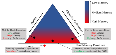
Figure 1: Visualization of optimization challenges of embedded deep reinforcement learning training. Arrow direction means better timing, better algorithm performance, and less memory usage. A higher red level represents higher memory pressure.

However, conducting on-device DRL training is fraught with unique challenges. As depicted by Figure 1, these challenges are fundamentally tied to the need for co-optimizing two frequently conflicting objectives: latency and algorithm performance, a task made more complex by the memory constraints inherent to embedded devices. Intrinsically, the DRL training process involves two critical components: batch execution and experience replay, each representing its own dimension of trade-off. Batch execution primarily pertains to the batch size parameter, which forms a crucial junction between timing and memory trade-offs. A larger batch size might accelerate the training process but increase memory consumption. On the other hand, experience replay entails a replay buffer size trade-off. Here, a larger buffer size can improve algorithm performance by providing more diverse experiences for training but can also cause memory issues due to the increased demand for storage. Optimizing these trade-offs independently could result in less-than-ideal outcomes, while co-optimizing them in a memory-agnostic manner may lead to significant memory pressure or even trigger Out-of-Memory (OOM) errors which in some severe cases cause the memory-limited embedded system (e.g., 16 GB memory for AGX Xavier) to fail. Therefore, a holistic memory-aware approach that addresses both dimensions of trade-off simultaneously becomes indispensable. To navigate this intricate multi-dimensional trade-off space and manage the inherent complexity of Real-time Deep Reinforcement Learning for Autonomous Robotics, in this paper, we present R³, which is designed to tackle the complex problem of on-device DRL training with careful consideration of timing, memory, and algorithmic performance. Our approach is composed of three innovative components. Firstly, we introduce a deadline-driven feedback loop, which dynamically assigns proper batch size for batch execution to balance memory and latency. Secondly, our approach includes efficient memory management, which applies task-specific memory optimizations to reduce memory footprint significantly. It allows for larger replay buffer sizes, enhancing algorithm performance in real-time embedded DRL while mitigating the risk of OOM occurrences. Finally, we incorporate a runtime coordinator, which synchronizes the interactions between the deadline-driven feedback loop, memory management, and other system components. This component, guided by heuristic analysis and a runtime profiler, dynamically adjusts memory resource reservations to meet hard resource constraints. These three components working together, enable R³ to effectively balance the trade-offs of latency, memory, and algorithm performance in a holistic manner, ultimately achieving real-time on-device DRL training.

Our approach, R³, has been deployed and tested across a range of DRL benchmarks [14, 15, 16] built upon different underlying frameworks [17, 18, 19, 20] to assess its efficacy with its application extending to three platforms, including a desktop and two embedded devices [21, 22]. Moreover, we highlight the practical usability of R³ by a further integration with a realistic autonomous car simulator [23]. Empirical results indicate that R³ achieves efficacy across diverse platforms, ensuring consistent latency performance and timing predictability with minimal overhead. Moreover, R³ showcases versatility by handling varied optimization goals and adapting to fluctuating systems scenarios. Notable achievements of R³ include:

• Cross-platform Efficacy: Our approach has demonstrated its efficacy in diverse environments across different platforms, including Classic Control [16], Atari [15], and DonkeyCar [14] environments. (Sec. IV-B)

• Latency predictability: Our proposed method consistently achieves timing predictability and satisfies deadlines across all benchmarks. (Sec. IV-B)

• Practical usability: Our user-friendly approach can be seamlessly integrated into existing practical complex deep reinforcement learning systems, such as DonkeyCar [14], without extensive modifications. (Sec. IV-C)

• Low overhead: The design and implementation of our method are highly efficient, resulting in negligible overhead on execution time and memory. (Sec. IV-D)

• Versatility: Our proposed framework exhibits a high degree of versatility, adeptly addressing diverse optimization goals and adapting to varying system scenarios. (Sec. IV-E)

II Background and Motivational Case Study

In this section, we present a series of illustrative case studies to elucidate the unique challenges associated with embedded deep reinforcement learning. These examples provide valuable insights into the limitations of existing approaches and highlight the potential pitfalls when naively extending them to address the problem context under consideration.

II-A Characteristics of Deep Reinforcement Learning

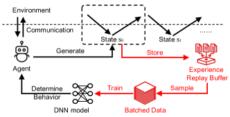
Figure 2: An overview of Deep Reinforcement Learning (DRL).

Deep Reinforcement Learning (DRL) is characterized by a combination of reinforcement learning (RL) algorithms and deep learning techniques (as shown in Figure 2), providing remarkable algorithm performance for extensive application prospects, particularly for intelligent robots [24, 25]. However, integrating DRL solutions into real-world autonomous embedded system-driven robots would be more challenging because robots are required to continuously, efficiently, and frequently train and retrain DRL models in order to adapt to new environments with strict timing and resource limitations. In such situations, meeting the real-time training deadlines is not merely a matter of budget adherence but a fundamental requirement to ensure system functionality, maintain up-to-date knowledge, and enhance accuracy. By emphasizing this, we make it clear that the timing sensitivity of DRL training extends beyond the offline workloads and is essential for a range of scenarios, especially those requiring real-time responses and continual learning.

To illustrate this need, consider the following real-world examples: (1) Autonomous navigation robots: DRL models must constantly adapt to dynamic road environments in the context of autonomous navigation robots. They are often required to learn and retrain based on new data and evolving environments. In such cases, meeting deadlines during the training phase ensures that the autonomous navigation robots’ decision-making system remains responsive and capable of handling new situations. (2) Search and Rescue Robots: In emergencies like disaster relief, robots need to navigate unpredictable challenges like damaged buildings or shifting debris. Quick training and updates to their DRL models allow them to adapt on-the-fly, ensuring they can effectively locate and assist those in need. (3) Drone Surveillance: Drones face a variety of challenges, from changing terrains in a forest to fluctuating weather conditions. Real-time DRL training ensures drones navigate these challenges efficiently, avoiding mishaps and ensuring effective monitoring.

To thoroughly comprehend the implications of Deep Reinforcement Learning (DRL) in embedded systems, it is essential to focus on two pivotal components (red parts in Figure 2) of DRL training: batch execution and replay buffer [26, 1, 2, 7, 5]. Batch execution involves processing multiple data samples in a single operation, fostering effective learning. The replay buffer, on the other hand, serves as a repository for past experiences, which are sampled for conducting minibatch training [1, 27]. These components significantly impact not only the algorithm’s application-level performance but also the system-level memory usage and latency [28, 4, 29]. This observation becomes particularly relevant in the context of real-time DRL systems, wherein training workloads consist of multiple time-bound tasks and subtasks, each encapsulating a complete DRL training episode. These tasks can be further divided into several subtasks, i.e., single-step-level minibatch training, with the flexibility for individual scheduling to meet specific end-to-end deadlines.

II-B Balancing Data Parallelism and Memory Usage: A Focus on Training Batch Size

In this subsection, we investigate the trade-off space between parallelism and memory usage in varying DRL training batch sizes, concentrating on its implications for both system-level and application-level performance. All the data in case studies are based on Classic Control [16], which is a set of classical control games for DRL, capable of simulating realistic robots and complex mechanical systems. Classic Control problem emphasizes the importance of control theory concepts, which corresponds to the key control components in robotic scenarios contexts.

As depicted in Figure 3, we perform a comprehensive analysis of performance metrics based on the autonomous learning library [19], which offers insights into the impact of batch size on performance.

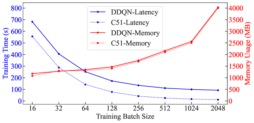
(a) Tradeoff for batch size

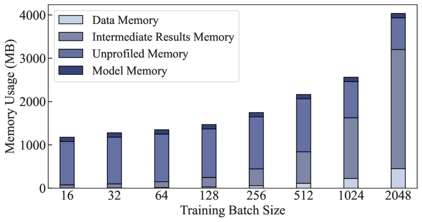
(b) Memory breakdown

Figure 3: Balancing data parallelism and memory usage.

Figure 3(a) highlights the trade-off space for training batch size, where data parallelism, the dominating factor affecting latency, can be improved with a larger training batch size, as long as it does not exceed the device’s computing capability. However, as the training batch size increases, memory usage consistently grows for different replay-based DRL algorithms. In Figure 3(b), we provide a memory breakdown analysis, which shows that data and intermediate result memory requirements increase significantly with larger batch sizes while model parameter memory remains minimal.

Consequently, the optimal batch size depends on the specific algorithm and the available computing resources. A thorough examination and optimization of batch size are necessary for more efficient and effective DRL training in resource-constrained situations.

Observation 1: The trade-off between parallelism and memory usage is vital for optimizing DRL training. Finding the proper balance through batch size adjustments can enhance algorithm performance while minimizing computing resource consumption.

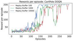
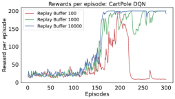
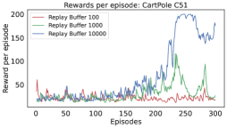
Figure 4: The deep reinforcement learning algorithm’s performance (rewards) gradually increases as the replay buffer size increases and convergence of the algorithms becomes faster while the memory usage increases significantly across different algorithms. The experiments are running based on Classic Control [16] CartPole environment. C51 refers to Categorical DQN.

TABLE I: Common resource-oblivious DRL training settings may cause serious out-of-memory (OOM) on resource-constrained embedded devices. “✓” refers OOM to happen.

Environment	Algorithm	Buffer Size	Batch Size	Peak Memory	Out-of-Memory
					Xavier	Orin
Classic Control [16]	DQN [1]	1,000,000	64	404.3MB	✗	✗
	DDQN [2]	1,000,000	64	404.3MB	✗	✗
	C51 [3]	1,000,000	32	404.2MB	✗	✗
Atari [15]	DQN [1]	1,000,000	32	40384.5MB	✓	✓
	DDQN [2]	1,000,000	32	40384.5MB	✓	✓
	C51 [3]	1,000,000	32	40384.5MB	✓	✓
DonkeyCar [14]	DQN [1]	100,000	128	35522.6MB	✓	✓
	DDQN [2]	100,000	128	35122.6MB	✓	✓
	C51 [3]	100,000	64	33329.8MB	✓	✓

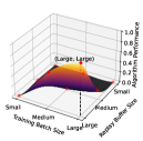
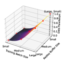
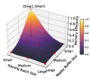
Figure 5: No silver bullet. Navigating the trade-offs: a three-dimensional analysis of performance metrics in embedded deep reinforcement learning and the challenge of out-of-memory issues. All data are normalized to the interval from zero to one to visualize the contribution of influence better.

II-C Balancing Algorithm Performance and Memory Usage: A Focus on Replay Buffer Size

In this subsection, we explore the trade-offs between algorithm performance and memory usage in DRL training with respect to replay buffer size. Figure 4 illustrates the clear tradeoff space between algorithm performance, exemplified by convergence time, and memory usage in DRL scenarios utilizing replay buffers. As the replay buffer size increases, the algorithm performance generally improves, leading many DRL training approaches to adopt large buffer sizes to boost algorithm performance. Additionally, cumulative rewards gained from DRL training rise with larger replay buffer sizes.

Nonetheless, it is essential to acknowledge that expanding replay buffer sizes also entails increased memory usage, potentially causing out-of-memory (OOM) issues, particularly in memory-constrained embedded devices. Table I presents default settings for various DRL benchmarks and examines the peak memory allocation for the buffer. Notably, some default settings for widely-used DRL algorithms could trigger OOM in powerful NVIDIA embedded devices.

Observation 2: Balancing algorithm performance and memory usage for replay buffer size are crucial in DRL training, particularly for memory-constrained embedded devices. A thorough examination of characteristics and trade-offs enables the optimization of performance while meeting practical memory constraints.

II-D Managing Complex Trade-offs under Practical System Scenarios: Balancing in the Three-dimensional Space

In light of the complexities of DRL and the trade-offs explored in the previous subsections, we now focus on the broader challenge of balancing conflicting characteristics in the three-dimensional space of DRL training under practical system scenarios.

As depicted in Figure 5, interestingly, patterns about the batch size and replay buffer size in different performance dimensions display vastly different behavior. This stark difference implies that DRL inherently involves conflicting characteristics. Simply co-optimizing some of these aspects may result in suboptimal solutions, underscoring the need for a more comprehensive and integrated approach. Moreover, practical challenges arise when considering resource-constrained embedded devices, where memory constraints may become a significant issue. Recall that simply combining the two 2-dimensional space optimization (as discussed in Sec.II-B and Sec.II-C) could exacerbate out-of-memory (OOM) problems.

To address such challenges, it is essential to carefully consider all characteristics in the three-dimensional space and their trade-offs while also taking into account the practical constraints of embedded devices. By adopting such a holistic approach, DRL training can achieve near optimal performance while managing these conflicting characteristics under practical system scenarios.

Observation 3: Managing trade-offs between various DRL training characteristics is a complex task due to multiple conflicting factors. A comprehensive approach considering all characteristics and performance objectvies is necessary, particularly for resource-constrained embedded devices.

III Methodology

III-A System Overview

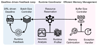
Figure 6: An overview of R³.

In response to the unique challenges of Real-time deep Reinforcement learning for Robotics outlined in Sec. II, we propose a comprehensive framework R³, illustrated in Figure 6. This framework encompasses two main components: a deadline-driven feedback loop and efficient memory management, which together facilitate the balance between the two-dimensional trade-off of batch size and replay buffer size. Moreover, a runtime coordinator is introduced to manage the complex three-dimensional trade-off under resource-constrained scenarios, ensuring the adaptation of different performance goals without conflicts. Each component is discussed in further detail below:

• Deadline-driven Feedback Loop: This component aims to balance memory constraints and latency (Sec. II-B). It dynamically assigns an intermediate deadline for each training episode based on the computation dynamics nature of DRL (as illustrated in Figure 7). Subsequently, it determines the optimal batch size that adheres to memory constraints while meeting the subtask deadline for the current training episode. If every subtask completes by its assigned intermediate deadline, the end-to-end deadline will be met.

• Efficient Memory Management: In addressing the challenges posed by memory-constrained embedded systems for DRL, efficient memory management is vital. Our proposed solution, corresponding to the trade-off discussed in Sec. II-C, implements task-specific memory optimizations to significantly reduce memory footprint. This enables larger replay buffer sizes for enhanced algorithm performance in real-time embedded DRL. Furthermore, we design an exception handler to eliminate unexpected out-of-memory (OOM) occurrences. Based on these underlying subcomponents, the buffer size controller can decide on demand how to assign replay buffer size.

• Runtime Coordinator: The runtime coordinator is essential for the seamless operation of R³, ensuring real-time DRL by synchronizing the interactions between the deadline-driven feedback loop, memory management, and other system components. Utilizing analytical modeling and a runtime profiler, the coordinator dynamically adjusts the resource reservation strategy in accordance with the actual system resource constraints. This guarantees that the runtime coordinator expertly maintains the delicate balance of factors required for achieving optimal DRL agent training.

By coherently integrating these three components, R³ provides a high-performance solution for training deep reinforcement learning agents in real-time. This enables rapid adaptation to dynamic and complex environments.

III-B Deadline-driven Feedback Loop

As emphasized in the preceding case study (Sec. II-B), achieving a balance between data parallelism and memory usage is vital for optimizing embedded DRL. Our goal is to meet end-to-end deadlines within hard memory constraints by adjusting the batch size. Intuitively, one possible approach is to partition subtasks and assign an appropriate intermediate deadline to each subtask. However, before designing a corresponding solution, it is necessary to consider how to partition the DRL workload and assign the intermediate deadline.

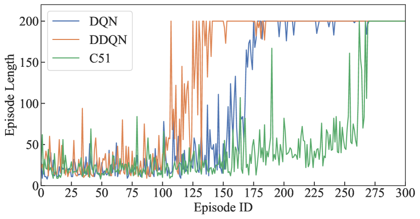
(a) Workload-induced dynamics

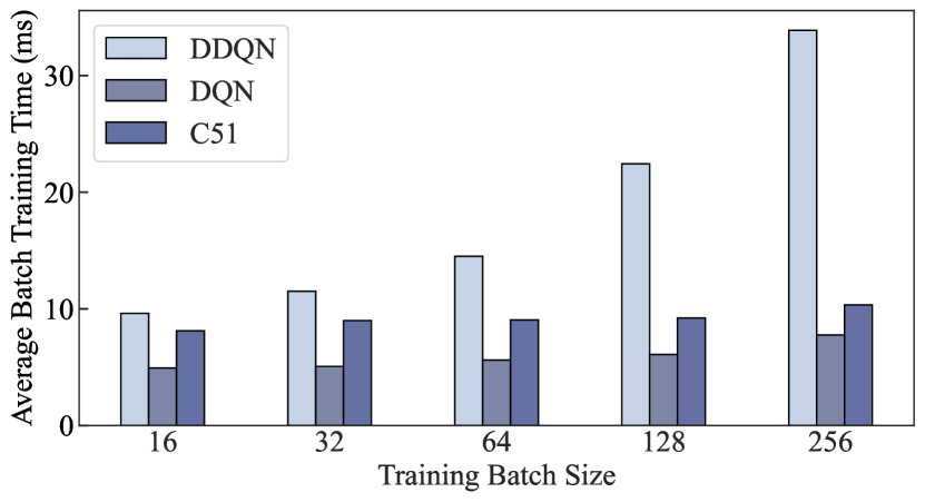
(b) Batching-induced dynamics

Figure 7: The computational dynamic nature of DRL emphasizes the need for dynamic intermediate deadline assignments.

Although DRL can be naturally divided into episodes, the computational dynamics of DRL workload add complexity to the assignment of reasonable intermediate deadlines. As illustrated in Figure 7, we leverage an example of DRL classic control [16] to show this point in two folds. At the DRL workload level, the computational cost of each natural computational subdivision unit (episode) varies over time, as depicted in Figure 7(a). The episode length was short at the beginning of DRL training; as the training progressed, the episode length gradually increased. Furthermore, examining finer-grained computation reveals that, since we aim to dynamically adjust the batch size, the computational cost of each batch (step) is also distinct, as depicted in Figure 7(b). This computational nature presents a further challenge to intermediate deadline assignments, which is hard to model without timing-consuming profiling. This implies that straightforwardly conducting a modeling-based optimization for all three dimensions may be infeasible across different DRL algorithms.

To address such a challenge, we propose an intuitive, practical deadline driven feedback loop mechanism that adapts to the varying computational dynamics of DRL workloads. The intuition is to directly adjust the batch size based on progress tracking without explicitly assigning intermediate deadlines. Specifically, we design to periodically assess the remaining time to dynamically adjust the training batch size incorporating temporal feedback information and thus meet the end-to-end deadline. Formally, as the DRL training process unfolds, two critical constraints often imposed are a data budget ($B$) and an end-to-end deadline ($D$). We keep track of the elapsed training time ($t_{i}$) and consumed budget ($s_{i}$) at the start of each episode $i$. We employ two trackers to monitor the progress of the DRL process: a timing tracker evaluates the ratio of elapsed training time to the given deadline, and a data tracker monitors the proportion of the consumed budget to the total budget. These ratios, denoted as $a$ and $b$ respectively, are given by $a=t_{i}/D$ and $b=s_{i}/B$.

These ratios serve as comparative indicators to guide the adjustment of the DRL process. If $a>b$, it indicates that the DRL training is lagging behind, necessitating acceleration by multiplying the current batch size by a scale factor $c$. Conversely, if $a<b$, it suggests the training is on track, thereby allowing for deceleration by dividing the batch size by the scale factor $c$. However, to maintain the stability of the DRL process, it is crucial to prevent the batch size from becoming excessively small or large. [1, 5, 26] As such, we confine the batch size within a specified range as per established DRL practices as follows:

$$b_{i+1}=\min(\max(b_{i},b_{\min}),4*b_{\min}).$$ (1)

Ultimately, it is critical to ensure that the DRL process complies with the hard memory constraint given by:

$$b_{i+1}=\min\left(b_{i+1},M_{batch}\cdot\frac{b_{base}}{M_{base}}\right).$$ (2)

Two key components in this context are $M_{base}$ and $M_{batch}$, both playing essential roles in memory reservation for batch execution during the scaling of minibatch size. The $M_{base}$ represents the memory reserved for batch execution considering a base minibatch size, denoted as $b_{base}$. This reservation is determined by the initial episode hyperparameter configuration, thereby serving as a reference point for subsequent adjustments. Conversely, $M_{batch}$ signifies the memory currently reserved for batch execution, a value that can dynamically vary in accordance with system constraints and requirements.

To further enhance the responsiveness, we integrate granular step-level adjustments within our feedback loop, enabling meticulous progress tracking at each training step for precise monitoring of elapsed time and budget expenditure. The detailed structure of this fine-grained deadline feedback loop aligns with the episode-level setup, facilitating seamless implementation without extensive modifications. Although this granular control promotes rapid adjustment to computational dynamics, it potentially introduces additional overhead that may affect training performance. Hence, the selection between episode-level and step-level adjustments is contingent upon specific DRL task requirements and available resources.

III-C Efficient Memory Management

As demonstrated in Sec. II-C, a larger replay buffer enhances algorithm performance but also demands more memory. The performance of DRL algorithms relies heavily on the quantity of data, which in turn depends on available memory resources. This is particularly relevant in resource-constrained embedded systems, where memory resources are limited and must be meticulously managed to avoid out-of-memory (OOM) issues. To address this challenge, we propose an efficient memory management scheme that contains memory optimization, an exception handler, and an application-level buffer size controller.

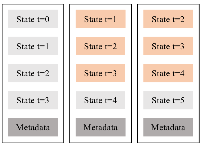
(a) Dummy replay buffer

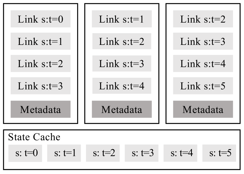
(b) Efficient replay buffer

Figure 8: Replay buffer memory optimization. The orange color indicates redundant data in the dummy replay buffer.

First, to target real-time embedded systems with stringent memory constraints, we propose underlying system-level DRL-task-specific optimizations for efficient memory management. First, we conduct a finer-grained analysis of the replay buffer and observe that the current caching mechanism of DRL training is inefficient. As illustrated in Figure 8(a), each data frame is stored in a tuple data structure (states, metadata) in the replay buffer, recording multiple time steps. It has to be admitted that such a dummy implementation can avoid frequent memory accesses and thus achieve higher parallelism, however, it would result in significant memory redundancy due to duplicated data shown in orange color. Ideally, each time step should maintain only one copy of data in the replay buffer. Based on this observation, we design and implement a simple yet efficient caching method that significantly reduces the memory footprint of the replay buffer, allowing for larger buffer sizes within memory-constrained embedded devices. As shown in Figure 8(b), we use a practical example of the Atari Breakout benchmark [1] to illustrate the ideal memory efficiency of our method. For each data frame of the dummy replay buffer implementation, each data frame stores 4 consecutive state information (i.e., 4 moments of RGB images with size (210,160), occupying size 4x210x160x3=403,200 bytes). In contrast, the metadata, containing action, reward, and done flag, occupies very little memory space (9 bytes) in total. Therefore, we use a contiguous memory for storing state information, while only storing soft links (4 bytes for each link) in the data frame. When the corresponding data frame is required, the corresponding tuple data is filled on demand. Our efficient replay buffer can ideally achieve about 75% less memory assumption to support the same length as a dummy replay buffer as in Figure 8, because in most data frames, three out of four pieces (orange) of state information are replaced with lightweight soft links.

Let $M_{replay}$ represent the total memory reserved for the replay buffer, $S_{state}$ represent the size of one state, $S_{metadata}$ represent the metadata size, and $N_{frames}$ represent the number of frames stored in a single data frame (in the Atari Breakout example, $N_{frames}=4$). The replay buffer size $r_{i}$ for training episode $i$ can be calculated as Eq. 3, where $S_{link}$ denotes the size of a soft link, which is used to reference the state information in the contiguous memory:

$$r_{i}=max\{M_{replay},(N_{frames}+i-1)*S_{state}+$$ (3)

$$(N_{frames}-1)\cdot i\cdot S_{link}+i\cdot S_{metadata}\}$$

Directly applying this efficient caching method could reduce memory redundancy, however, it could introduce substantial overhead since it necessitates more memory access, potentially harming data parallelism in DRL training. Inspired by recent work [30], we optimize the training process with non-blocking data prefetching to hide latency. These task-specific optimizations enable real-time embedded DRL training to achieve larger replay buffer sizes for improved algorithm performance while minimizing side effects on data parallelism. To handle the possibility of unexpected out-of-memory (OOM) issues caused by memory interference or other unforeseen circumstances, we propose to design an exception handler mechanism. This mechanism can monitor memory usage during runtime and promptly react when an OOM exception is detected. The handler can temporarily scale down the memory reservations for both batch execution and replay buffer, which allows the system to recover gracefully from the OOM situation. Furthermore, it can record the OOM events and adjust the memory allocation strategy accordingly, ensuring the system remains robust under memory interference.

Specifically, we show part of the code example of a standard DDQN training step (as shown in Listing 1). We use a multi-threading technique to hide the latency of data prefetching (line 4) and thus achieve a better training step latency. Based on the above optimizations, the buffer size controller could calculate the current maximum replay buffer size based on the given memory limit and dynamically allocate or free memory at runtime.

⬇

1def _train(self):

2 if self._should_train():

3 # sample transitions from buffer

4 (states, actions, rewards, next_states, weights) = self.replay_buffer.sample(self.minibatch_size)

5 # forward pass

6 values = self.q(states, actions)

7 # compute targets and loss

8 next_actions = torch.argmax(self.q.no_grad(next_states), dim=1)

9 targets = rewards + self.discount_factor * self.q.target(next_states, next_actions)

10 loss = self.loss(values, targets, weights)

11 # backward pass

12 self.q.reinforce(loss)

13 # update replay buffer

14 self.replay_buffer.update()

Listing 1: An example code of DRL training.

III-D Runtime Coordinator

The Runtime Coordinator in R³ is a pivotal component devised to address the intricate triadic trade-off between algorithm performance, memory efficiency, and data parallelism (as outlined in Sec. II-D). This component serves to orchestrate the execution of various system aspects, including the deadline-driven feedback loop and efficient memory management, thereby enabling smooth real-time DRL training. The coordination is executed through heuristic analysis, taking into consideration the outputs from the aforementioned system components alongside system-level resource constraints and performance objectives.

Memory reservations $M_{batch}$ and $M_{replay}$ are adjusted using a heuristic formulation that factors in the system’s current performance and memory constraints. For episode $i$, the episode runtime is denoted as $t_{i}$, and the cumulative reward is $R_{i}$. Two scaling factors, $\alpha$ and $\beta$, are employed to fine-tune the memory reservations based on the system’s performance:

$$\alpha =\frac{\gamma t_{i}}{\sum\limits_{j=1}^{\gamma}{t_{i-j}}}$$ (4)

$$\beta =\frac{\gamma R_{i}}{\sum\limits_{j=1}^{\gamma}{R_{i-j}}}$$

Here, $t_{i}$ is the runtime of episode $i$, $R_{i}$ is the cumulative reward at the i-th episode, $\gamma$ is a hyperparameter, and $R_{i-\gamma}$ is the cumulative reward $\gamma$ steps prior to the i-th episode. $\gamma$’s role is to control the reward comparison span. By modulating $\gamma$, the algorithm can be adjusted to focus on short-term or long-term reward trends, influencing the training process and potentially enhancing overall performance. $\alpha$ and $\beta$ track latency and algorithm performance dynamically. To this end, the memory reservations for batch execution and replay buffer are then updated based on $\alpha$ and $\beta$ :

$$M_{batch}^{new}=M_{batch}\cdot(1+\max(\alpha-1,0)\cdot(1-\min(\beta,1)))$$ (5)

$$M_{replay}^{new}=M_{replay}\cdot(1+\min(\alpha,1)\cdot\max(1-\beta,0))$$

Here, $M_{batch}^{new}$ and $M_{replay}^{new}$ represent the updated memory reservations for batch execution and replay buffer, respectively. This adjustment mechanism increases batch memory if the episode runtime is shorter than the subtask deadline and the cumulative reward is increasing relative to the training loss, while reducing replay buffer memory. To ensure total memory usage does not exceed system constraints, the sum of $M_{batch}^{new}$ and $M_{replay}^{new}$ must be checked against the available memory budget. If it exceeds the limit, memory reservations are proportionally scaled down to fit within the constraints. Let’s denote $M$ as the total available memory. We want to proportionally distribute $M$ between $M_{batch}$ and $M_{replay}$. First, we calculate the proportion of each reservation to the total desired memory, i.e., the sum of $M_{batch}^{new}$ and $M_{replay}^{new}$. Then, we allocate the memory in proportion to these ratios. The resulting equations are:

$$M_{batch}^{final}=M\cdot\frac{M_{batch}^{new}}{M_{batch}^{new}+M_{replay}^{new}}$$ (6)

$$M_{replay}^{final}=M\cdot\frac{M_{replay}^{new}}{M_{batch}^{new}+M_{replay}^{new}}$$

Here, $M_{batch}^{final}$ and $M_{replay}^{final}$ are the final memory reservations for batch execution and replay buffer, respectively. These equations ensure that the total memory used is exactly $M$, and that it is distributed in proportion to the desired reservations for batch execution and the replay buffer.

Let’s consider different scenarios to illustrate the behavior of the memory reservation system:

• Timing Inefficiency: When $\alpha>1$ (indicating an episode runtime exceeding its subtask deadline), there is an increase in the batch memory allocation ($M_{batch}^{new}$). This allocation is unaffected by performance ($\beta\geq 1$), as efficient operation negates the need for additional batch processing memory.

• Performance Deterioration: An increase in replay buffer memory allocation ($M_{replay}^{new}$) is observed when $\beta<1$, signifying performance deterioration. Temporal efficiency ($\alpha\leq 1$) neutralizes the adjustment to batch memory ($M_{batch}^{new}$), as an efficient runtime eliminates the need for more replay buffer memory.

• Maintaining Optimal Performance: Under optimal conditions of both runtime and performance ($\alpha\leq 1$, $\beta\geq 1$), the memory reservations for batch execution and replay buffer remain constant. This indicates the system is running efficiently, thus no need to adjust memory allocations.

• Balanced Trade-off: In the event of both inefficient runtime ($\alpha>1$) and performance deterioration ($\beta<1$), there is a compensatory increase in both $M_{batch}^{new}$ and $M_{replay}^{new}$. Despite this, the overall memory usage must remain within system constraints, necessitating a proportional reduction in memory reservations if required.

These illustrative cases demonstrate the adaptability of the memory reservation system in response to different performance conditions. By dynamically adjusting $M_{batch}$ and $M_{replay}$, the system can address diverse challenges and maintain a balanced trade-off between timing performance and algorithm performance, all within the constraints of the available memory budget.

III-E Algorithm Details

Algorithm 1 R³ framework

1:Input: hyperparameter $m$; hyperparameter $\gamma$; end-to-end deadline $D$; training budget $B$; maximal training episode $N$; Data frame information $I$; training budget $C$;

2:Initialize memory reservation {$M_{batch},M_{replay}$} with $m$;

3:Initialize spent training cost $c$ with $0$;

4:for each episode $i\in N$ do

5:     Batch size $b_{i}\leftarrow$BatchSizeControl$(D,B,M_{batch})$;

6:     Replay size $r_{i}\leftarrow\textsc{ReplayControl}(I,M_{replay})$;

7:     if $i>0\text{ and }r_{i}<r_{i-1}$ then

8:         ShrinkReplayBuffer($r_{i}$);

9:         GarbageCollection();

10:     else

11:         ExpandReplayBuffer($r_{i}$);      

12:     Synchronization();

13:     if IsCoarseGrained() then

14:         Training Logs $s$ $\leftarrow$ VanillaTraining();

15:     else

16:         Training Logs $s$ $\leftarrow$ DynamicTraining();      

17:     Update spent training cost $c\leftarrow c+s[cost]$;

18:     if $c>=C$ or meet early exit condition then

19:         exit();      

20:     Update memory reservation {$M_{batch},M_{replay}$} $\leftarrow$ RuntimeCoordinator $(s,\gamma,\{M_{batch},M_{replay}\})$

The overall workflow of the R³ framework is presented in Algorithm 1. For each DRL training episode, the batch size is initially determined in accordance with Eq. 2 in Sec. III-B. Subsequently, the replay buffer size is computed by Eq. 3 in Sec. III-C. Following this, a series of replay buffer size adjustments, memory garbage collection, and synchronization operations are executed on-demand to maintain system correctness. Next, the coarse-grained algorithm is trained according to the standard process, while the fine-grained algorithm slightly adjusts the batch size of each training step. Training progress is checked afterward to avoid overspending the training budget. It’s worth mentioning that inspired by early stopping techniques [31], once the training meets the algorithm performance goal($K$ consecutive episodes rewards consistently no smaller than the targeted algorithm performance $R^{*}$), the training process will exit early to minimize latency. Lastly, based on the acquired training logs, the runtime coordinator dynamically adjusts the memory resources allocated to batch execution and replay buffer management by Eq. 6. This enables the R³ framework to effectively balance the trade-offs among data parallelism, memory usage, and algorithm performance, resulting in a more efficient and adaptive system.

IV Evaluation

IV-A Experimental Setup

Testbeds. We choose three different platforms aiming to demonstrate the cross-platform compatibility of our design as shown in Table II. These platforms comprise one desktop configuration along with two NVIDIA embedded platforms, motivated by the widespread adoption of NVIDIA hardware in deployed autonomous systems, particularly in the domains of autonomous driving [32, 33] and robotics [34, 35, 36, 37].

TABLE II: Hardware platforms used in our experiments.

	Desktop	NVIDIA AGX Xavier	NVIDIA AGX Orin
CPU	Intel(R) Core(TM)	8-core NVIDIA	8-core Armv8.2
	i7-10700K CPU	Carmel Armv8.2	Cortex-A78AE
	@ 3.80GHz	64-bit CPU	64-bit CPU
GPU	NVIDIA GTX 3060	NVIDIA Volta GPU	NVIDIA Ampere GPU
Memory	DDR4 16GBx2	16GB LPDDR4x	32GB LPDDR5
Storage	1TB SSD	32GB eMMC	64GB eMMC

Benchmarks. To thoroughly evaluate our solution, we have selected three deep reinforcement learning benchmark environments, as detailed in Table III. These environments encompass various application areas and are widely used in the research community. Note that we evaluate two representative DRL benchmarks, Atari [1] and Classic Control [16], integrated with widely used autonomous-learning-library(ALL) [19]. We use these Classic Control and Atari to evaluate the overall effectiveness and versatility of R³. Additionally, to demonstrate the robustness of our solution in real-world practical scenarios, we further conduct a practical case study by integrating our approach into autonomous navigation scenarios, empowered by a high-resolution simulator DonkeyCar [14]. In our experiments, we assess the performance of three well-known and widely implemented DRL algorithms: DQN [1], DDQN [2], and C51 [3]. These algorithms provide a comprehensive comparison of our solution’s efficacy and adaptability across different learning methods and application domains. We set hyperparameter $b_{min}$ strictly following the MAX-A preset settings, $m$ refers to each platform’s maximal available memory, $\gamma$ to 4. We set hyperparameter maximal episode number $N$ to 10000 for all environments, data budget the same as MAX-A preset setting, and early exit parameter $K$ to 10 for all benchmark, $R^{*}$ to 200, 300, and 1000 for Classic Control, Atari, and DonkeyCar.

TABLE III: Deep reinforcement learning benchmark environments used in our experiments.

Benchmark ID	Description
Atari [1]	A well-known environment for video game-based deep reinforcement learning research, featuring a collection of Atari 2600 games.
Classic Control [16]	A set of classical control games for deep reinforcement learning research, capable of simulating robots and complex mechanical systems.
DonkeyCar [14]	A practical simulated deep reinforcement learning environment for training autonomous driving agents and deploying to real-world platforms.

Metrics. This paper evaluates two main types of metrics. The first set reflects latency predictability, which evaluates the throughput by end-to-end latency and real-time performance indicators using task deadline miss rates. Moreover, end-to-end deadlines for DRL training are based on the worst-case execution time (WCET), and task deadlines are based on the proportional intermediate deadline assignment. The second set of metrics corresponds to algorithm performance, measuring widely adopted maximal and average cumulative rewards.

Baselines. We compare R³ to the following approaches:

• MAX-A: To maximize the algorithm performance, we directly adopt preset hyperparameters in the autonomous learning library (ALL) [19], which is an object-oriented novel deep reinforcement learning (DRL) library designed for PyTorch [38]. The creators have incorporated high-quality reference implementations of modern DRL algorithms and provided ease of use API, and pre-defined hyperparameter sets for best algorithm performance.

• MAX-P: MAX-P, or maximal data parallelism, denotes a high-efficiency mode that enables concurrent data processing to achieve peak performance. For fair comparisons, we implement MAX-P strictly following the implementation of ALL [19] to exploit the computational resources and maximize throughput in DRL training scenarios.

• R³: Our proposed solution is implemented at various DRL training granularities: R³_episode for coarse-grained episode-level and R³_step for fine-grained step-level implementation.

Scheduling Policy. In on-device DRL training, there is only one DRL training job running at a time because the training task is extremely resource-demanding for both computation and memory resources, and the GPU resource is often limited (e.g., typically only one GPU device available for most desktop and embedded settings). Therefore, such scenarios cannot be optimized through multi-task scheduling. We thus applied FIFO scheduling in all cases. Deadline miss rates are calculated task-wise based on the proportional intermediate deadline assignment policy.

IV-B Overall Effectiveness

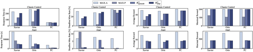
Figure 9: Overall effectiveness of R³ on the C51 algorithm evaluated on four different resource-constrained intelligent robotic systems. R³ auto balances throughput, timing correctness, and algorithm performance.

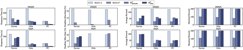
Figure 10: R³ evaluated on more different DRL algorithms on the Classic Control benchmark.

We measure the overall effectiveness of R³ across three platforms. Since our design concerns latency predictability and algorithm efficacy, we measure both constraints and compare against strong baselines based on widely used DRL evaluating benchmarks autonomous-learning-library (ALL) [19].

Latency predictability. Figure 9 shows timing performance comparisons. In the Classic Control benchmark, R³ outperforms MAX-A, with average execution time improvements of 39.3%, 8.2%, and 9.0% on Xavier, Orin, and PC. This improvement is attributed to our memory management, which increases memory access slightly but enhances timing optimization. On the PC, latencies are similar, maybe due to the high computation capabilities of desktop GPU meeting the relatively small benchmark Classic Control. Other platforms show notable timing differences, indicating the efficacy of our solution on embedded systems. The deadline miss rate further emphasizes this, with R³ improving over MAX-A by 15.0%, 1.7%, and 7.8% on Xavier, Orin, and PC. On the Atari benchmark, R³ balances timing correctness and algorithm performance, outperforming MAX-A by 71.9% and 5.8%. However, MAX-P on Xavier is slower, possibly due to the Atari benchmark’s longer duration and Xavier’s older Linux kernel affecting CPU scheduling. Figure 11 breaks down response times, showing R³ consistently outperforms MAX-A in timeliness. The empirical results demonstrate that our proposed R³ qualitatively has significantly better timeliness than MAX-A, avoiding potentially high-tailed latency.

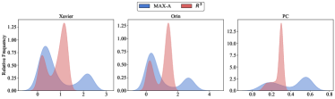
Figure 11: Episode-level response time histogram across different platforms. R³ ensure significantly better timing correctness than MAX-A qualitatively.

Algorithm Efficacy. The last two columns of Figure 9 display algorithm performance comparisons. On the Classic Control benchmark, R³ almost obtains a very close to optimal algorithm performance (MAX-A) by on average 100.0% and 82.7% on average rewards and maximal rewards, while outperforming MAX-P by a large margin on average by 76.5% and 133.6% on average rewards and maximal rewards, respectively. Note that the theoretical upper bound of maximal reward for Classic Control is 200; both MAX-A and R³ consistently reach this maximal value during training. This quantitatively validates the effectiveness of our co-optimization, especially for training a usable DRL algorithm under strict time and memory constraints. On the Atari benchmark, R³ auto-balances the timing correctness and algorithm performance. Specifically, R³ achieves on average by 49.7% and 50.2% on the average rewards and maximal rewards than MAX-A, but largely outperforms on average by 1521.1% and 1297.8% on the average rewards and maximal rewards than MAX-P. This supports the validity R³ and further evidences the resilience of our design. Furthermore, to demonstrate quantitatively the algorithm performance between different methods, we plot the per-episode cumulative rewards during the training process, as shown in Figure 12. It can be observed that MAX-P runs out of data budget too early (green curves), so the training lasts only a very small number of episodes and therefore leads to very poor algorithm performance. In contrast, our proposed R³ selects proper bath size in the batch execution, thus reaching algorithm performance consistently better than MAX-P and nearly approaching empirically optimal MAX-A.

Evaluated on more DRL algorithms. Our method, R³, was further evaluated on two additional algorithms (refer to Figure 10). Specifically, for the DDQN algorithm, R³ performs better than MAX-A for execution time by 73.9%, 79.4%, and 81.1% on Xavier, Orin, and PC. Also, R³ performs better than MAX-P for maximal rewards by 94.2%, 110.5%, and 140.1% on Xavier, Orin, and PC. Additionally, R³ performs better than MAX-P for average rewards by 94.2%, 133.1%, and 141.0% on Xavier, Orin, PC. Additionally, for the DQN algorithm, R³ performs better than MAX-A for execution time by 133.1%, 102.0%, and 101.3% on Xavier, Orin, and PC. Also, R³ performs better than MAX-P for maximal rewards by 83.5%, 83.8%, and 60.0% on Xavier, Orin, and PC. Additionally, R³ performs better than MAX-P for average rewards by 256.8%, 84.3%, and 68.3% on Xavier, Orin, and PC. Our efficient memory optimization yields supreme latency performance of R³, even outperforming MAX-P in DDQN and DQN. Note that R³ exhibited a markedly low deadline miss rate for both DRL algorithms, suggesting its adaptability and efficacy in enhancing real-time performance (see Table IV).

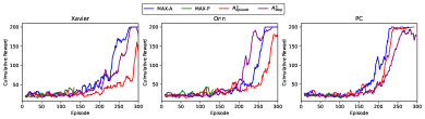
Figure 12: Episode-level reward curves across different platforms. The algorithm performance of R³ is consistently better than MAX-P and close to MAX-A (empirical optimal).

TABLE IV: Deadline miss rate on DDQN and DQN algorithms. The best values are in bold.

	Solution	Xavier	Orin	PC
DDQN	MAX-P	8.3%	2.4%	17.7%
	MAX-A	57.9%	54.5%	56.0%
	R3episode	0.0%	0.0%	0.0%
	R3step	0.0%	0.0%	0.0%
DQN	MAX-P	13.8%	0.0%	55.6%
	MAX-A	67.1%	55.4%	51.4%
	R3episode	39.6%	0.0%	0.0%
	R3step	43.6%	0.0%	0.0%

Cross-platform overall effectiveness: R³ effectively addresses all challenges outlined in Sec. II for resource-constrained intelligent robotic systems. It auto-balances throughput, timing correctness, and algorithm performance in DRL training across different platforms.

IV-C A Practical Case study: Autonomous Navigation via DRL

To empirically evaluate the effectiveness of our proposed approach, R³, in real-world DRL applications for robotics, we conducted a comprehensive case study centered on autonomous navigation. We selected DonkeyCar [14] as the platform for this case study, a high-resolution environment based on the x86 Unity3D autonomous navigation simulator [39], as displayed in Figure 13. DonkeyCar was chosen due to its relevance in investigating the deployment of DRL-based control systems in real-world robotics contexts. Several real-world autonomous driving cars are built upon DonkeyCar library [40, 23] based on TensorFlow framework [18]. To successfully incorporate DRL training into this platform, we implement a highly optimized networking module that facilitates the seamless execution of DRL training natively on advanced embedded systems (Xavier and Orin). The integration of these robust systems underscores the real-world feasibility and performance of R³ in robotic contexts, highlighting its potential for wider adoption in various robotic applications.

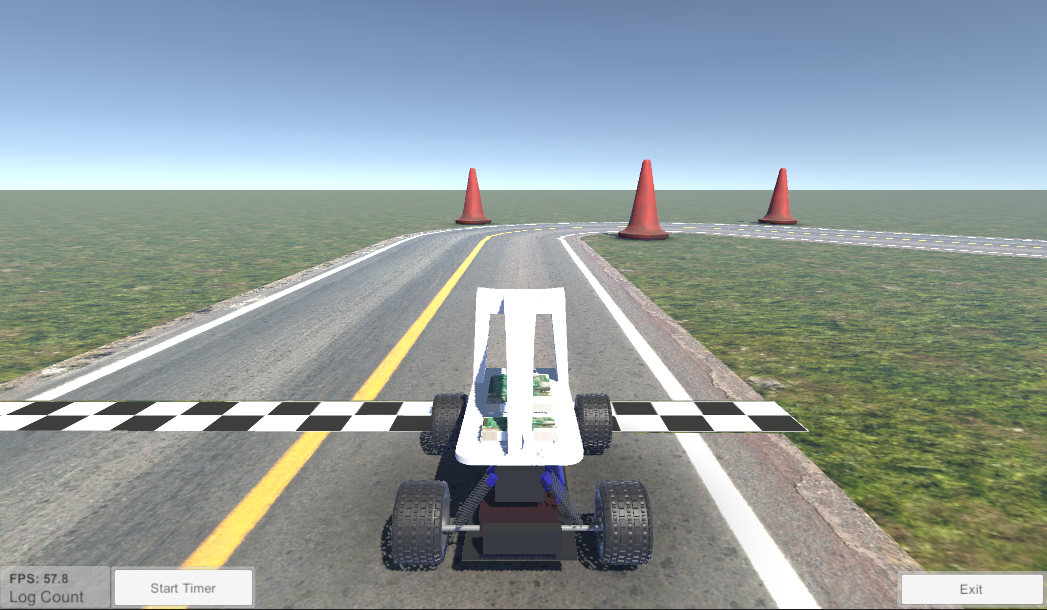
(a) Generated track

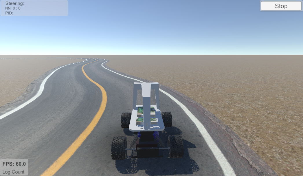
(b) Generated road

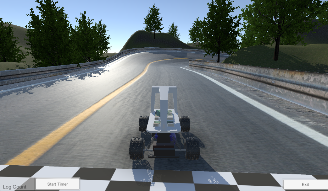
(c) Mountain track

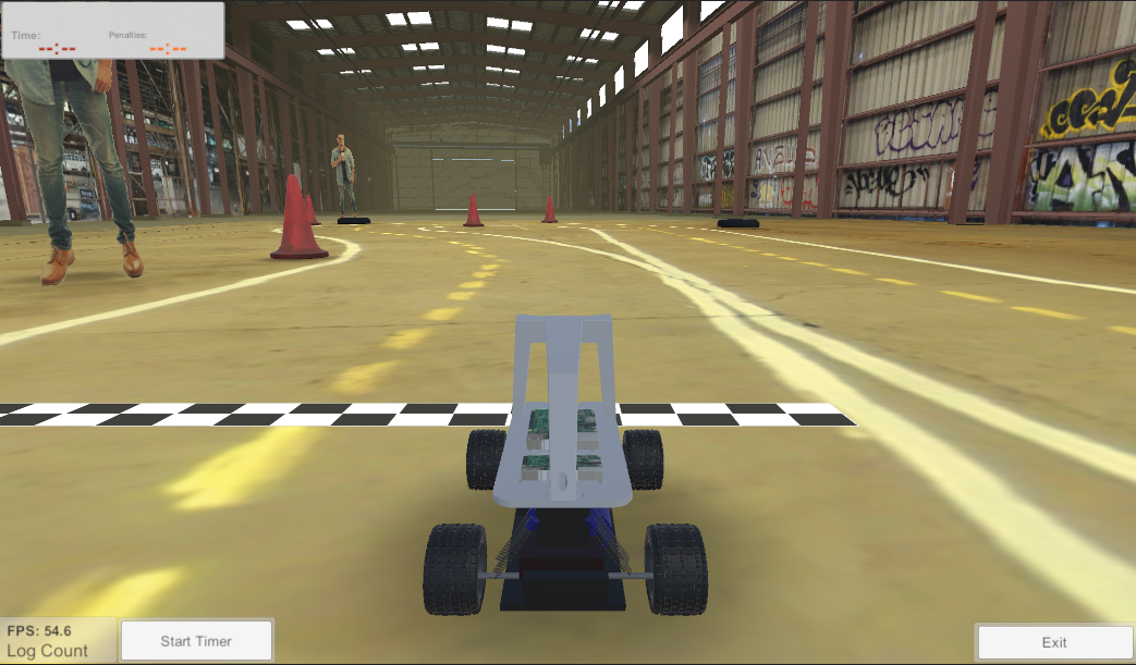
(d) Warehouse track

Figure 13: DonkeyCar [14] driven high-resolution autonomous navigation simulator for evaluating DRL algorithm.

DonkeyCar [14] processes 60 FPS high-resolution RGB images as streaming camera inputs, raising a significant memory challenge when conducting on-device DRL training. Table V presents the results of the DDQN algorithm implementation on DonkeyCar, showcasing a range of evaluation metrics. Specifically, we report latency, FPS to describe throughput, data budget consumption percentage to describe the relative percentage of training completion, and maximal rewards R_max and average rewards R_avg to describe algorithm performance.

TABLE V: Quantitative results on DonkeyCar simulator. DPR implies data processing rate, Reward_max implies maximal episode rewards, and Reward_avg implies average episode rewards. ^∗ implies OOM occurs.

Platform	Solution	Latency$(\downarrow)$	DPR$(\uparrow)$	Budget$(\uparrow)$	Rmax$(\uparrow)$	Ravg$(\uparrow)$
Xavier	MAX-P	64.7∗	1423.8	0.2%	116.6	59.8
	MAX-A	3619.4∗	742.0	41.9%	1343.2	157.3
	R3episode	7525.9	850.4	100.0%	532.7	79.1
	R3step	7429.1	861.5	100.0%	544.1	80.2
Orin	MAX-P	4918.0	1301.3	100.0%	29.4	7.3
	MAX-A	8341.0∗	653.7	85.2%	1303.8	156.9
	R3episode	8416.18	760.4	100.0%	598.6	67.0
	R3step	8205.23	780.0	100.0%	588.5	70.2

Results demonstrate that R³ adeptly balances both latency predictability and algorithm efficacy without incurring out-of-memory (OOM) problems on both platforms; while OOM occurs for MAX-A on both platforms and MAX-P on Xavier. R³’s data processing rate (DPR) exceeds MAX-A by an average of 16.6%, while R³ lags behind MAX-P by an average of 40.4%. This is because R³ provides a smaller batch size than MAX-P. In terms of algorithm performance, R³ significantly outperforms MAX-P, with maximal and average rewards better by 872.9% and 1140.3% in the challenging autonomous navigation task. Still, R³ trades off certain algorithm performance by 57.2% and 52.8% on maximal and average rewards, mainly due to reserving smaller memory for replay buffer compared to MAX-A.

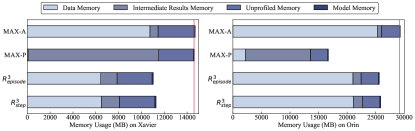
Figure 14: Memory breakdown on DonkeyCar evaluated on two embedded devices. The red line represents the OOM point.

A deeper dive into R³’s memory efficiency, as shown in Figure 14, reveals its strengths. MAX-A heavily consumes memory in data storage due to high-res RGB images in its replay buffer. As this buffer expands, memory use grows uncontrollably, causing OOM errors. In contrast, MAX-P’s memory consumption spikes in batch execution, storing numerous intermediate activations, leading to OOM errors on Xavier. However, R³ optimally manages memory in both data storage and batch execution. Its innovative replay buffer design allows for a larger size within the same memory constraints, enhancing algorithmic output. R³ also dynamically adjusts batch sizes during training, striking a balance between timing requirements and memory constraints, ensuring effective DRL training within these boundaries.

Pratical usability: This case study demonstrates the integration effectiveness of R³ on practical robotic applications. R³ significantly reduces the memory footprint by efficient memory optimization, ensuring the usability of R³ in embedded robotic DRL training scenarios.

IV-D Overhead Analysis

We further break down the overhead of R³ for different platforms regarding execution time and memory usage.

TABLE VI: Detailed average runtime execution overhead (s) and percentage of applying R³ for each benchmark.

Platform	Benchmark	Feedback	MM	Coord
Xavier	Classic Control	0.30 (0.15%)	0.11 (0.05%)	0.07 (0.04%)
	Atari	3.68 (0.01%)	10.22 (0.01%)	0.16 (0.01%)
	DonkeyCar	0.35 (0.01%)	41.95 (0.56%)	0.09 (0.01%)
Orin	Classic Control	0.14 (0.05%)	0.29 (0.11%)	0.06 (0.02%)
	Atari	1.55 (0.03%)	11.04 (0.02%)	0.08 (0.01%)
	DonkeyCar	0.22 (0.01%)	115.8 (1.41%)	0.04 (0.01%)
PC	Classic Control	0.05 (0.09%)	0.10 (0.19%)	0.01 (0.02%)
	Atari	0.99 (0.01%)	8.93 (0.02%)	0.04 (0.01%)
	DonkeyCar	N/A	N/A	N/A

Execution Overhead. Table VI details the average execution overhead for each component: deadline-driven feedback loop (Feedback), replay memory management (MM), and runtime coordinator (Coord) across platforms. The system’s execution overhead remains under 1.43%, underscoring our method’s efficiency. The feedback loop has a minimal overhead, peaking at 3.68s in Atari. The runtime coordinator also maintains a low overhead, at most 0.16s and 0.01%. Conversely, memory management has a higher overhead, reaching 115.8s and 1.41% on Orin, due to increased memory access in our strategy. Yet, this is counterbalanced by memory optimization techniques like non-blocking data prefetching, enhancing the overall system performance.

TABLE VII: Detailed memory overhead and percentage of applying R³ for each benchmark.

	(a) Overhead upon Framework			(b) Overall Overhead Ratio
	Feedback	MM	Coord	Xavier	Orin	PC
Classic Control	5 KB	160 KB	3 KB	0.001%	0.001%	0.001%
Atari	50 KB	15.6 MB	10 KB	0.975%	0.488%	0.488%
DonkeyCar	12 KB	1.6 MB	15 KB	0.010%	0.005%	0.005%

Memory Overhead. Table VII showcases the memory overhead of R³, both in absolute terms and as a percentage. The overhead remains below 1% on all platforms, making R³ ideal for memory-limited autonomous systems. While emphasizing memory efficiency, R³ may compromise latency. Future work might focus on minimizing memory access or enhancing caching strategies for better memory management.

Low overhead: R³’s efficient implementation introduces low overhead, making it a lightweight deployment solution for optimizing on-device DRL training.

IV-E Adaptability to Different System Scenarios

As a complement to the overall effectiveness, we investigate the adaptability of the proposed R³. We focus on the adaptation of both variable deadline and variable computational interference in the following angles.

Adaptability to Variant Deadlines. We examine the adaptability of R³ to variant end-to-end deadlines in Figure 15. This figure depicts the outcomes, demonstrating that R³ can dynamically adjust to variant end-to-end deadlines. Thus it can sustain a highly predictable task-level tail latency within a defined range of computational interference. This evidences the resilience of R³ as a solution to different timing constraints.

Adaptability to Variant Computational Interference. We examine DRL training based on R³ alongside a computationally demanding background workload, namely FFmpeg video decoding, to explore the adaptability of R³ to computational interference. We varied the interference workload intensity by modifying the video’s output resolution. Specifically, 720P, 1080P, and 2K decoding resolutions were employed to represent light, heavy, and malicious interference. Figure 15 depicts the outcomes, demonstrating that R³ can dynamically adjust to computational workload, thereby sustaining a highly predictable task-level tail latency within a defined range of computational interference. Thus, it ensures the fulfillment of end-to-end deadlines.

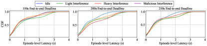
Figure 15: Episode-level latency CDF for varying deadline configuration and interference workloads intensity on Xavier.

Versatility: R³ consistently maintains its effectiveness across different system scenarios, including various deadline settings and interference workloads. This adaptability ensures robustness and resilience, regardless of timing or computational constraints.

V Related Work and Discussion

Deep Reinforcement Learning (DRL) has gained significant attention due to its ability to learn complex tasks and adapt to dynamic environments, making it particularly suitable for recent robotics applications [41, 9, 8, 42, 43] and future robots with complex deep learning techniques [44, 45, 46, 47, 48, 49, 50, 51, 52, 53, 54, 55]. The foundation of DRL rests on DQN’s introduction [1] and its subsequent extensions tailored to robotics, including DDQN[2], C51 [3], and others. While newer algorithms such as PPO [5], TRPO [6], SAC [7] have emerged, the real-time capabilities of DRL algorithms largely remain an untapped domain. Notably, while a few studies propose new DRL algorithms that can provide faster response times [56, 57, 58], R³ could optimize performance of given DRL algorithms without modifying the algorithms themselves. Recent research has explored dynamic adjustments of training parameters, such as batch size [59] and replay buffer size [60], to enhance algorithmic performance. However, these approaches, being agnostic to system constraints, risk causing catastrophic out-of-memory (OOM) errors as illustrated in Figure 1. In contrast, by considering the unique properties of system constraints and DRL, R³ effectively avoids OOM errors while achieving the goal of efficient real-time DRL training.

Recently, real-time ROS schedulers have emerged equipped with a suite of optimization strategies [61, 62, 63, 64, 65, 66, 67]. Our emphasis remains mainly on application-layer application for DRL training, but the potential of integrating more ROS optimizations remains an exciting prospect for future exploration.

Although considerable progress has been made in addressing real-time deep learning inference [68, 69, 70, 71, 72, 73, 74, 30, 75, 76], unfortunately, adapting these techniques directly to the DRL training scenario poses new challenges since the complexity and resource-demanding characteristics of training. This paper empirically explores these challenges and introduces a novel framework for on-device DRL training.

Limitations of R³. R³ provides optimization in a static hardware context, but there still exists space to get performance gains from software-hardware synergy [77]. Moreover, R³ focus is on DRL training that utilizes replay buffers, leaving the optimization for replay-buffer-free DRL algorithms [78] unaddressed. Additionally, despite validations on the DonkeyCar simulator [14] for R³, physical-world implementations may introduce additional unpredictability, such as sensor noise, dynamic lighting conditions, unpredictable environmental changes, and unmodeled physical interactions. To understand how well R³ works in the real world, a promising future direction is actual autonomous systems integration[79, 80, 81, 82, 83].

VI Conclusion

This study introduces the novel framework, R³, which is specifically designed to ensure timing predictability for executing deep reinforcement learning (DRL) training workloads in GPU-enabled autonomous embedded systems. The comprehensive nature of R³ allows for the seamless optimization of both timing and algorithm performance while simultaneously adhering to stringent memory constraints. This is achieved by incorporating a thorough understanding of DRL workload characteristics as well as utilizing real-time system feedback information. Through rigorous experimentation, we have demonstrated that R³ consistently showed a significant reduction in OOM errors, effective latency handling, and maintenance of competitive algorithm performance, marking a stride in the realm of embedded real-time DRL.

References

- [1] V. Mnih, K. Kavukcuoglu, D. Silver, A. A. Rusu, J. Veness, M. G. Bellemare, A. Graves, M. Riedmiller, A. K. Fidjeland, G. Ostrovski et al., “Human-level control through deep reinforcement learning,” nature, vol. 518, no. 7540, pp. 529–533, 2015.
- [2] H. Van Hasselt, A. Guez, and D. Silver, “Deep reinforcement learning with double q-learning,” in Proceedings of the AAAI conference on artificial intelligence, vol. 30, no. 1, 2016.
- [3] M. G. Bellemare, W. Dabney, and R. Munos, “A distributional perspective on reinforcement learning,” in International conference on machine learning. PMLR, 2017, pp. 449–458.
- [4] T. Schaul, J. Quan, I. Antonoglou, and D. Silver, “Prioritized experience replay,” arXiv preprint arXiv:1511.05952, 2015.
- [5] J. Schulman, F. Wolski, P. Dhariwal, A. Radford, and O. Klimov, “Proximal policy optimization algorithms,” arXiv preprint arXiv:1707.06347, 2017.
- [6] J. Schulman, S. Levine, P. Abbeel, M. I. Jordan, and P. Moritz, “Trust region policy optimization,” International conference on machine learning, pp. 1889–1897, 2015.
- [7] T. Haarnoja, A. Zhou, P. Abbeel, and S. Levine, “Soft actor-critic: Off-policy maximum entropy deep reinforcement learning with a stochastic actor,” in International conference on machine learning. PMLR, 2018, pp. 1861–1870.
- [8] G. Kahn, A. Villaflor, B. Ding, P. Abbeel, and S. Levine, “Self-supervised deep reinforcement learning with generalized computation graphs for robot navigation,” 2018 IEEE International Conference on Robotics and Automation (ICRA), pp. 1–8, 2018.
- [9] X. B. Peng, P. Abbeel, S. Levine, and M. van de Panne, “Deepmimic: Example-guided deep reinforcement learning of physics-based character skills,” ACM Transactions on Graphics (TOG), vol. 37, no. 4, p. 143, 2018.
- [10] A. Ayub and C. Fendley, “Few-shot continual active learning by a robot,” in NeurIPS, 2022. [Online]. Available: http://papers.nips.cc/paper\_files/paper/2022/hash/c58437945392cec01e0c75ff6cef901a-Abstract-Conference.html
- [11] M. Riemer, S. C. Raparthy, I. Cases, G. Subbaraj, M. P. Touzel, and I. Rish, “Continual learning in environments with polynomial mixing times,” in NeurIPS, 2022. [Online]. Available: http://papers.nips.cc/paper\_files/paper/2022/hash/89c61fce5a8b73871d1c4073f486b134-Abstract-Conference.html
- [12] M. Aggravi, A. A. S. Elsherif, P. R. Giordano, and C. Pacchierotti, “Haptic-enabled decentralized control of a heterogeneous human-robot team for search and rescue in partially-known environments,” IEEE Robotics and Automation Letters, vol. 6, no. 3, pp. 4843–4850, 2021.
- [13] L. Heintzman, A. Hashimoto, N. Abaid, and R. K. Williams, “Anticipatory planning and dynamic lost person models for human-robot search and rescue,” in 2021 IEEE International Conference on Robotics and Automation (ICRA). IEEE, 2021, pp. 8252–8258.
- [14] T. Kramer, “Openai gym environments for donkey car,” 2023.
- [15] M. G. Bellemare, Y. Naddaf, J. Veness, and M. Bowling, “The arcade learning environment: An evaluation platform for general agents,” Journal of Artificial Intelligence Research, vol. 47, pp. 253–279, 2013.
- [16] A. G. Barto, R. S. Sutton, and C. W. Anderson, “Neuronlike adaptive elements that can solve difficult learning control problems,” IEEE Transactions on Systems, Man, and Cybernetics, vol. SMC-13, no. 5, pp. 834–846, 1983.
- [17] A. Paszke, S. Gross, F. Massa, A. Lerer, J. Bradbury, G. Chanan, T. Killeen, Z. Lin, N. Gimelshein, L. Antiga et al., “Pytorch: An imperative style, high-performance deep learning library,” Advances in neural information processing systems, vol. 32, 2019.
- [18] M. Abadi, P. Barham, J. Chen, Z. Chen, A. Davis, J. Dean, M. Devin, S. Ghemawat, G. Irving, M. Isard et al., “Tensorflow: a system for large-scale machine learning,” in 12th USENIX symposium on operating systems design and implementation (OSDI 16), 2016, pp. 265–283.
- [19] C. Nota, “The autonomous learning library,” https://github.com/cpnota/autonomous-learning-library, 2020.
- [20] G. Brockman, V. Cheung, L. Pettersson, J. Schneider, J. Schulman, J. Tang, and W. Zaremba, “Openai gym,” 2016.
- [21] NVIDIA, “Jetson agx xavier,” https://developer.nvidia.com/embedded/jetson-agx-xavier, 2020.
- [22] ——, “Jetson agx orin,” https://www.nvidia.com/en-us/autonomous-machines/embedded-systems/jetson-orin/, 2022.
- [23] robocarstore, “Donkey car s1,” https://www.robocarstore.com/products/donkey-car-starter-kit, 2023.
- [24] K. Arulkumaran, M. P. Deisenroth, M. Brundage, and A. A. Bharath, “Deep reinforcement learning: A brief survey,” IEEE Signal Processing Magazine, vol. 34, no. 6, pp. 26–38, 2017.
- [25] T. Chen, T. Moreau, Z. Jiang, L. Zheng, E. Yan, M. Cowan, H. Shen, L. Wang, Y. Hu, L. Ceze et al., “Tvm: An automated end-to-end optimizing compiler for deep learning,” arXiv preprint arXiv:1802.04799, 2018.
- [26] T. P. Lillicrap, J. J. Hunt, A. Pritzel, N. Heess, T. Erez, Y. Tassa, D. Silver, and D. Wierstra, “Continuous control with deep reinforcement learning,” arXiv preprint arXiv:1509.02971, 2015.
- [27] M. McCloskey and N. J. Cohen, “Catastrophic interference in connectionist networks: The sequential learning problem,” in Psychology of learning and motivation. Elsevier, 1989, vol. 24, pp. 109–165.
- [28] D. Horgan, J. Quan, D. Budden, G. Barth-Maron, M. Hessel, H. Van Hasselt, and D. Silver, “Distributed prioritized experience replay,” arXiv preprint arXiv:1803.00933, 2018.
- [29] P. Henderson, R. Islam, P. Bachman, J. Pineau, D. Precup, and D. Meger, “Deep reinforcement learning that matters,” in Proceedings of the AAAI conference on artificial intelligence, vol. 32, no. 1, 2018.
- [30] M. Ji, S. Yi, C. Koo, S. Ahn, D. Seo, N. D. Dutt, and J. Kim, “Demand layering for real-time DNN inference with minimized memory usage,” in IEEE Real-Time Systems Symposium, RTSS 2022, Houston, TX, USA, December 5-8, 2022. IEEE, 2022, pp. 291–304. [Online]. Available: https://doi.org/10.1109/RTSS55097.2022.00033
- [31] Y. Yao, L. Rosasco, and A. Caponnetto, “On early stopping in gradient descent learning,” Constructive Approximation, vol. 26, no. 2, pp. 289–315, 2007.
- [32] S. Kato, S. Tokunaga, Y. Maruyama, S. Maeda, M. Hirabayashi, Y. Kitsukawa, A. Monrroy, T. Ando, Y. Fujii, and T. Azumi, “Autoware on board: Enabling autonomous vehicles with embedded systems,” in 2018 ACM/IEEE 9th International Conference on Cyber-Physical Systems (ICCPS). IEEE, 2018, pp. 287–296.
- [33] B. Kisačanin, “Deep learning for autonomous vehicles,” in 2017 IEEE 47th International Symposium on Multiple-Valued Logic (ISMVL). IEEE, 2017, pp. 142–142.
- [34] A. Popov, P. Gebhardt, K. Chen, R. Oldja, H. Lee, S. Murray, R. Bhargava, and N. Smolyanskiy, “Nvradarnet: Real-time radar obstacle and free space detection for autonomous driving,” arXiv preprint arXiv:2209.14499, 2022.
- [35] NVIDIA, “Duckiebot (db-j),” https://get.duckietown.com/products/duckiebot-db21, 2022.
- [36] ——, “Sparkfun jetbot ai kit,” https://www.sparkfun.com/products/18486, 2022.
- [37] ——, “Waveshare jetbot ai kit,” https://www.amazon.com/Waveshare-JetBot-AI-Kit-Accessories/dp/B07V8JL4TF/, 2022.
- [38] A. Paszke, S. Gross, F. Massa, A. Lerer, J. Bradbury, G. Chanan, T. Killeen, Z. Lin, N. Gimelshein, L. Antiga et al., “Pytorch: An imperative style, high-performance deep learning library,” Advances in neural information processing systems, vol. 32, 2019.
- [39] J. K. Haas, “A history of the unity game engine,” Diss. Worcester Polytechnic Institute, vol. 483, no. 2014, p. 484, 2014.
- [40] D. Car, “Donkey docs,” https://docs.donkeycar.com/guide/build_hardware, 2023.
- [41] J. Guo, A. Li, and C. Liu, “Backdoor detection and mitigation in competitive reinforcement learning,” arXiv preprint arXiv:2202.03609, 2022.
- [42] S. He, S. Han, S. Su, S. Han, S. Zou, and F. Miao, “Robust multi-agent reinforcement learning with state uncertainty,” Transactions on Machine Learning Research, 2023.
- [43] S. Nikkhoo, Z. Li, A. Samanta, Y. Li, and C. Liu, “Pimbot: Policy and incentive manipulation for multi-robot reinforcement learning in social dilemmas,” arXiv preprint arXiv:2307.15944, 2023.
- [44] S. I. Serengil and A. Ozpinar, “Lightface: A hybrid deep face recognition framework,” in 2020 Innovations in Intelligent Systems and Applications Conference (ASYU). IEEE, 2020, pp. 23–27. [Online]. Available: https://doi.org/10.1109/ASYU50717.2020.9259802
- [45] Z. Li, X. He, Y. Li, S. Nikkhoo, W. Yang, L. Thiele, and C. Liu, “Mimonet: Multi-input multi-output on-device deep learning,” arXiv preprint arXiv:2307.11962, 2023.
- [46] M. Afarin, C. Gao, S. Rahman, N. Abu-Ghazaleh, and R. Gupta, “Commongraph: Graph analytics on evolving data,” in Proceedings of the 28th ACM International Conference on Architectural Support for Programming Languages and Operating Systems, Volume 2, 2023, pp. 133–145.
- [47] Y. Chen, Y. Zhang, C. Zhang, G. Lee, R. Cheng, and H. Li, “Revisiting self-training for few-shot learning of language model,” arXiv preprint arXiv:2110.01256, 2021.
- [48] Y. Chen, Y. Zhang, B. Wang, Z. Liu, and H. Li, “Generate, discriminate and contrast: A semi-supervised sentence representation learning framework,” arXiv preprint arXiv:2210.16798, 2022.
- [49] X. Gao, C. Gupta, and H. Li, “Automatic lyrics transcription of polyphonic music with lyrics-chord multi-task learning,” IEEE/ACM Transactions on Audio, Speech, and Language Processing, vol. 30, pp. 2280–2294, 2022.
- [50] ——, “Polyscriber: Integrated fine-tuning of extractor and lyrics transcriber for polyphonic music,” IEEE/ACM Transactions on Audio, Speech, and Language Processing, 2023.
- [51] S. Chen, Z. Song, M. Haque, C. Liu, and W. Yang, “Nicgslowdown: Evaluating the efficiency robustness of neural image caption generation models,” in Proceedings of the IEEE/CVF Conference on Computer Vision and Pattern Recognition, 2022, pp. 15 365–15 374.
- [52] S. Chen, H. Khanpour, C. Liu, and W. Yang, “Learning to reverse dnns from ai programs automatically,” arXiv preprint arXiv:2205.10364, 2022.
- [53] S. Chen, M. Haque, C. Liu, and W. Yang, “Deepperform: An efficient approach for performance testing of resource-constrained neural networks,” in Proceedings of the 37th IEEE/ACM International Conference on Automated Software Engineering, 2022, pp. 1–13.
- [54] Z. Li, B. Yin, T. Yao, J. Guo, S. Ding, S. Chen, and C. Liu, “Sibling-attack: Rethinking transferable adversarial attacks against face recognition,” in Proceedings of the IEEE/CVF Conference on Computer Vision and Pattern Recognition, 2023, pp. 24 626–24 637.
- [55] Y. Chen, S. Chen, Z. Li, W. Yang, C. Liu, R. T. Tan, and H. Li, “Dynamic transformers provide a false sense of efficiency,” arXiv preprint arXiv:2305.12228, 2023.
- [56] P. Thodoroff, W. Li, and N. D. Lawrence, “Benchmarking real-time reinforcement learning,” in NeurIPS 2021 Workshop on Pre-registration in Machine Learning. PMLR, 2022, pp. 26–41.
- [57] S. Ramstedt and C. Pal, “Real-time reinforcement learning,” in Advances in Neural Information Processing Systems 32: Annual Conference on Neural Information Processing Systems 2019, NeurIPS 2019, December 8-14, 2019, Vancouver, BC, Canada, H. M. Wallach, H. Larochelle, A. Beygelzimer, F. d’Alché-Buc, E. B. Fox, and R. Garnett, Eds., 2019, pp. 3067–3076. [Online]. Available: https://proceedings.neurips.cc/paper/2019/hash/54e36c5ff5f6a1802925ca009f3ebb68-Abstract.html
- [58] J. García and F. Fernández, “A comprehensive survey on safe reinforcement learning,” Journal of Machine Learning Research, vol. 16, no. 1, pp. 1437–1480, 2015.
- [59] A. Nikulin, V. Kurenkov, D. Tarasov, D. Akimov, and S. Kolesnikov, “Q-ensemble for offline rl: Don’t scale the ensemble, scale the batch size,” arXiv preprint arXiv:2211.11092, 2022.
- [60] W. Fedus, P. Ramachandran, R. Agarwal, Y. Bengio, H. Larochelle, M. Rowland, and W. Dabney, “Revisiting fundamentals of experience replay,” in International Conference on Machine Learning. PMLR, 2020, pp. 3061–3071.
- [61] X. Jiang, D. Ji, N. Guan, R. Li, Y. Tang, and Y. Wang, “Real-time scheduling and analysis of processing chains on multi-threaded executor in ROS 2,” in IEEE Real-Time Systems Symposium, RTSS 2022, Houston, TX, USA, December 5-8, 2022. IEEE, 2022, pp. 27–39. [Online]. Available: https://doi.org/10.1109/RTSS55097.2022.00013
- [62] R. Li, N. Guan, X. Jiang, Z. Guo, Z. Dong, and M. Lv, “Worst-case time disparity analysis of message synchronization in ROS,” in IEEE Real-Time Systems Symposium, RTSS 2022, Houston, TX, USA, December 5-8, 2022. IEEE, 2022, pp. 40–52. [Online]. Available: https://doi.org/10.1109/RTSS55097.2022.00014
- [63] H. Teper, M. Günzel, N. Ueter, G. von der Brüggen, and J. Chen, “End-to-end timing analysis in ROS2,” in IEEE Real-Time Systems Symposium, RTSS 2022, Houston, TX, USA, December 5-8, 2022. IEEE, 2022, pp. 53–65. [Online]. Available: https://doi.org/10.1109/RTSS55097.2022.00015
- [64] T. Blaß, D. Casini, S. Bozhko, and B. B. Brandenburg, “A ROS 2 response-time analysis exploiting starvation freedom and execution-time variance,” in 42nd IEEE Real-Time Systems Symposium, RTSS 2021, Dortmund, Germany, December 7-10, 2021. IEEE, 2021, pp. 41–53. [Online]. Available: https://doi.org/10.1109/RTSS52674.2021.00016
- [65] Y. Tang, Z. Feng, N. Guan, X. Jiang, M. Lv, Q. Deng, and W. Yi, “Response time analysis and priority assignment of processing chains on ROS2 executors,” in 41st IEEE Real-Time Systems Symposium, RTSS 2020, Houston, TX, USA, December 1-4, 2020. IEEE, 2020, pp. 231–243. [Online]. Available: https://doi.org/10.1109/RTSS49844.2020.00030
- [66] H. Choi, Y. Xiang, and H. Kim, “Picas: New design of priority-driven chain-aware scheduling for ROS2,” in 27th IEEE Real-Time and Embedded Technology and Applications Symposium, RTAS 2021, Nashville, TN, USA, May 18-21, 2021. IEEE, 2021, pp. 251–263. [Online]. Available: https://doi.org/10.1109/RTAS52030.2021.00028
- [67] T. Blaß, A. Hamann, R. Lange, D. Ziegenbein, and B. B. Brandenburg, “Automatic latency management for ROS 2: Benefits, challenges, and open problems,” in 27th IEEE Real-Time and Embedded Technology and Applications Symposium, RTAS 2021, Nashville, TN, USA, May 18-21, 2021. IEEE, 2021, pp. 264–277. [Online]. Available: https://doi.org/10.1109/RTAS52030.2021.00029
- [68] S. Bateni and C. Liu, “Neuos: A latency-predictable multi-dimensional optimization framework for dnn-driven autonomous systems,” in 2020 USENIX Annual Technical Conference (USENIX ATC 20), 2020, pp. 371–385.
- [69] W. Kang, K. Lee, J. Lee, I. Shin, and H. S. Chwa, “Lalarand: Flexible layer-by-layer cpu/gpu scheduling for real-time dnn tasks,” in 2021 IEEE Real-Time Systems Symposium (RTSS). IEEE, 2021, pp. 329–341.
- [70] Y. Xiang and H. Kim, “Pipelined data-parallel cpu/gpu scheduling for multi-dnn real-time inference,” in 2019 IEEE Real-Time Systems Symposium (RTSS). IEEE, 2019, pp. 392–405.
- [71] S. Bateni and C. Liu, “Apnet: Approximation-aware real-time neural network,” in 2018 IEEE Real-Time Systems Symposium (RTSS). IEEE, 2018, pp. 67–79.
- [72] H. Zhou, S. Bateni, and C. Liu, “S^ 3dnn: Supervised streaming and scheduling for gpu-accelerated real-time dnn workloads,” in 2018 IEEE Real-Time and Embedded Technology and Applications Symposium (RTAS). IEEE, 2018, pp. 190–201.
- [73] S. Bateni, H. Zhou, Y. Zhu, and C. Liu, “Predjoule: A timing-predictable energy optimization framework for deep neural networks,” in 2018 IEEE Real-Time Systems Symposium (RTSS). IEEE, 2018, pp. 107–118.
- [74] V. Nigade, P. Bauszat, H. E. Bal, and L. Wang, “Jellyfish: Timely inference serving for dynamic edge networks,” in IEEE Real-Time Systems Symposium, RTSS 2022, Houston, TX, USA, December 5-8, 2022. IEEE, 2022, pp. 277–290. [Online]. Available: https://doi.org/10.1109/RTSS55097.2022.00032
- [75] J. Jiang, Z. Luo, C. Hu, Z. He, Z. Wang, S. Xia, and C. Wu, “Joint model and data adaptation for cloud inference serving,” in 42nd IEEE Real-Time Systems Symposium, RTSS 2021, Dortmund, Germany, December 7-10, 2021. IEEE, 2021, pp. 279–289. [Online]. Available: https://doi.org/10.1109/RTSS52674.2021.00034
- [76] J. S. Jeong, J. Lee, D. Kim, C. Jeon, C. Jeong, Y. Lee, and B.-G. Chun, “Band: coordinated multi-dnn inference on heterogeneous mobile processors,” in Proceedings of the 20th Annual International Conference on Mobile Systems, Applications and Services, 2022, pp. 235–247.
- [77] J. Zhang, M. Imani, and E. Sadredini, “Bp-ntt: Fast and compact in-sram number theoretic transform with bit-parallel modular multiplication,” arXiv preprint arXiv:2303.00173, 2023.
- [78] T. Schaul, J. Quan, I. Antonoglou, and D. Silver, “Prioritized experience replay,” in 4th International Conference on Learning Representations, ICLR 2016, 2016.
- [79] S. He, Y. Wang, S. Han, S. Zou, and F. Miao, “A robust and constrained multi-agent reinforcement learning framework for electric vehicle amod systems,” arXiv preprint arXiv:2209.08230, 2022.
- [80] S. He, S. Han, and F. Miao, “Robust electric vehicle balancing of autonomous mobility-on-demand system: A multi-agent reinforcement learning approach,” arXiv preprint arXiv:2307.16228, 2023.
- [81] I. Gog, S. Kalra, P. Schafhalter, J. E. Gonzalez, and I. Stoica, “D3: a dynamic deadline-driven approach for building autonomous vehicles,” in Proceedings of the Seventeenth European Conference on Computer Systems, 2022, pp. 453–471.
- [82] F. Favarò, S. Eurich, and N. Nader, “Autonomous vehicles’ disengagements: Trends, triggers, and regulatory limitations,” Accident Analysis & Prevention, vol. 110, pp. 136–148, 2018.
- [83] “Baidu Apollo team (2017), Apollo: Open Source Autonomous Driving, howpublished = https://github.com/apolloauto/apollo, note = Accessed: 2019-02-11.”