Entanglement Routing over Networks with Time Multiplexed Repeaters

Abstract

Quantum networks will be able to service consumers with long distance entanglement by use of repeater nodes that can both generate external Bell pairs with their neighbors, iid with probability $p$, as well as perform internal Bell State Measurements (BSMs) which succeed with some probability $q$. The actual values of these probabilities is dependent upon the experimental parameters of the network in question. While global link state knowledge is needed to maximize the rate of entanglement generation between any two consumers, this may be an unreasonable request due to the dynamic nature of the network. This work evaluates a local link state knowledge, multi-path routing protocol that works with time multiplexed repeaters that are able to perform BSMs across different time steps. This study shows that the average rate increases with the time multiplexing block length, $k$, although the initial latency also increases. When a step function memory decoherence model is introduced so that qubits are held in the quantum memory for a time exponentially distributed with mean $\mu$, an optimal $k$ ($k_{\text{opt}}$) value appears. As $p$ decreases or $\mu$ increases the value of $k_{\text{opt}}$ increases. This value is such that the benefits from time multiplexing are balanced with the increased risk of losing a previously established entangled pair.

=-15pt

I Introduction

Quantum networks will have the ability to generate, distribute, and process quantum information along with classical data. These networks can connect quantum computers, sensors, simulators, etc., and enable consumers to share entangled connections on demand over potentially large distances. There are various applications for entangled qubits shared over quantum networks, such as provably-secure communication [1, 2], entanglement-enhanced sensing [3, 4, 5, 6, 7], and distributed quantum computing [8]. To enable these, it is important to be able to reliably and quickly transmit quantum bits from one point in a network to another in order to establish entanglement between distant users.

A quantum network is comprised of two main components: nodes, which are equipped with entanglement sources, quantum memories, quantum processors, and the ability to classically communicate, and edges, which connect neighboring nodes via channels that transmit entangled (typically photonic) qubits, such as optical fibers. The nodes, such as those illustrated in Fig. 1 by the blue squares, can be consumers wanting to utilize entanglement for some application or quantum repeaters, which are fundamental for the successful distribution of entanglement across large distances. The rate of quantum entanglement across an optical fiber decays exponentially with the distance between communicating parties [9]. However, when utilizing these intermediate nodes, the magnitude of the exponent can be decreased by breaking up the total distance between consumers, which helps to mitigate the loss incurred from the transmitting medium [10, 11, 12, 13].

Quantum links are maximally-entangled two-qubit states called Bell states shared along edges when two neighboring nodes each successfully store one half of a Bell pair in their quantum memories. The generation of these links has a probability $p$ of succeeding. This value should be set based on the actual physical hardware and may encompass optical loss of the link, as well as detector and memory inefficiencies. Repeaters in this paper are quantum switches [14, 12], which can simultaneously attempt to form entangled links with neighboring nodes and dynamically choose on which links to perform an entanglement swap on by using local network information. A swap is most commonly implemented by performing a Bell State Measurement (BSM) on qubits held within a repeater with a probability of success denoted by $q$. If successful, this results in the corresponding qubits held at the repeater’s neighbors to become entangled. However, if the measurement fails, both Bell states the repeater shared with its neighbors are lost.

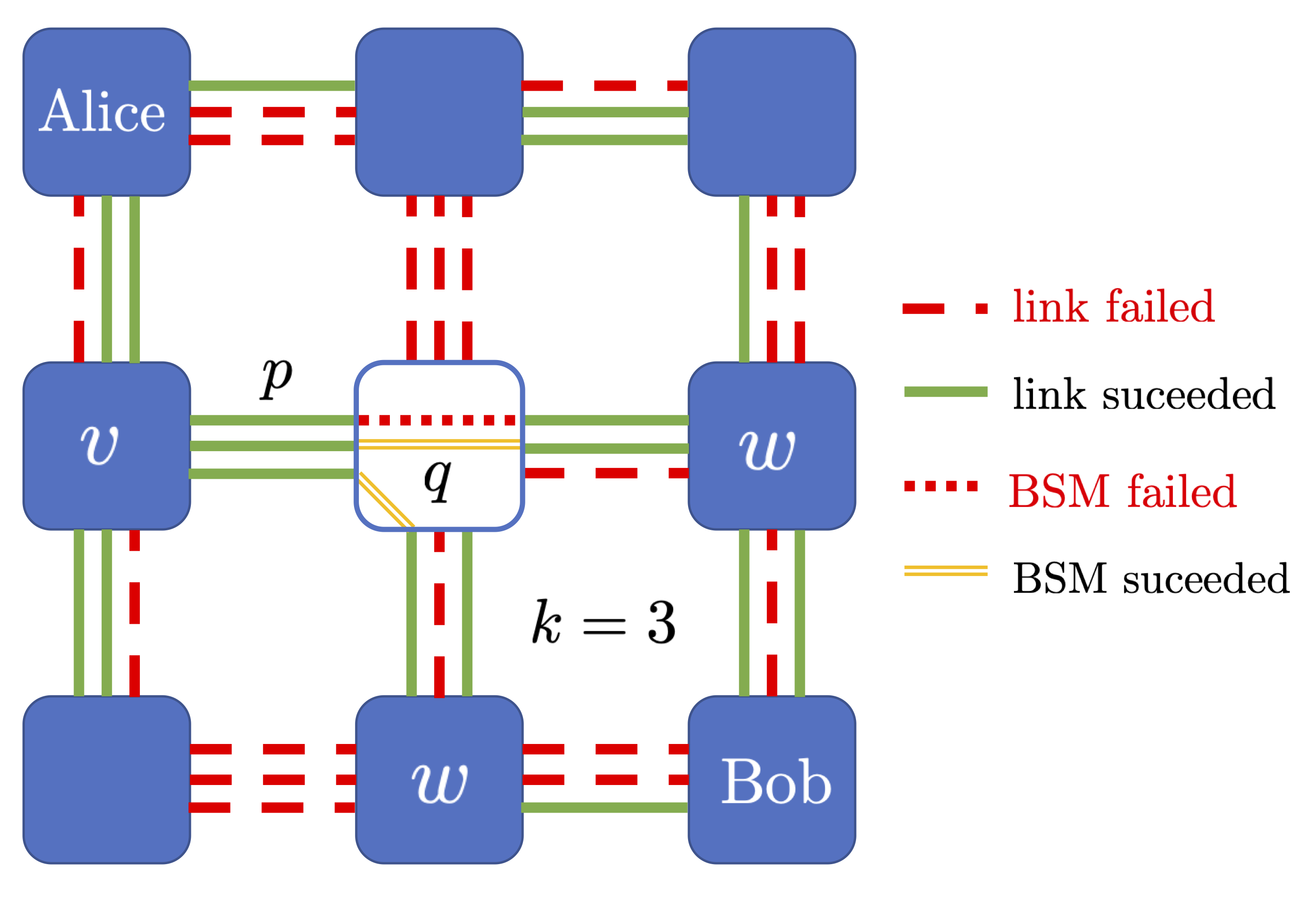
Figure 1: A snapshot of the distance-based routing protocol being implemented on a 3x3 grid network for $k=3$. The outcomes of the external phase are all shown here, while the center repeater node highlights the decisions made during the internal phase. The repeater node labeled $v$ is the neighbor closest to Alice, while both of the nodes labeled $w$ are closest to Bob. All of the repeater nodes in the network are simultaneously making swapping decisions, although only the decisions of the center node are shown here.

Increasing the rate of entanglement distribution for networks under different constraints is crucial to the usefulness of quantum networks. The probabilistic nature of link generation means that different instances, or snapshots, of the network, will have different links present/absent. Global link state knowledge is needed by a protocol to ensure that two consumers, Alice and Bob, share the maximum number of Bell pairs possible given the initial snapshot. However, global link state knowledge is often not possible as quantum networks can spread out across large distances giving rise to large latencies due to classical communication. Quantum memories cannot support this condition as they have very short storage lifetimes. Routing protocols have been proposed to lower latency and therefore the requirements on quantum memories by creating of virtual graphs of entangled links before or as consumers request entangled pairs [15, 16]. To further reduce this latency, [17] created a protocol that combined multi-path routing and local link state knowledge to distribute Bell pairs to consumers. It was seen to provide rates larger than those achievable by a single linear repeater chain and only required that each repeater knew the physical topology of the network and the outcomes of their own entanglement generation attempts. Further exploration of distance-based routing schemes can be found in [18, 19, 20]. Distillation protocols and routing were analyzed in [21] to maximize the distillable entanglement between consumers.

When quantum repeaters are equipped with the ability to perform GHZ-projective measurements, under a certain range of $p$ and $q$ values, the rate of entanglement distribution becomes distance independent, in contrast with the typical exponential decay observed with distance [22]. Further improved multipartite entanglement distribution schemes can be found in [23, 24].

Time multiplexed link generation is currently being explored to increase the rate of distribution of entangled qubits. It has recently been shown that time-multiplexed repeater nodes, equipped with the ability to perform BSMs across different time steps, allow for a sub-exponential decay with distance [25]. This result is otherwise unattainable with just spatial or spectral multiplexing. Time multiplexing has also been combined with GHZ-projective measurements, and it has been shown that distance independent rates can be achieved over larger region in the $p$-$q$ space than that without multiplexing [26].

In this paper, we combine the benefits of multipath routing with local link state knowledge as discussed above with time multiplexed repeaters to further improve the rate of entanglement distribution. This protocol will be explicitly explained in Section II. The remainder of the paper will focus on simulated results. In Section III we will evaluate this protocol on networks where memories have infinite coherence time. Under such a condition, time multiplexing only serves to improve the average rate. We discuss the impact that the quantum network’s structure, as well as the location of consumers, has on the performance of our protocol. In Section IV we will reduce the coherence time of our quantum memories, and show that there exists an optimal amount of time multiplexing dependent on the conditions of the network. Lastly, we will offer concluding thoughts in Section V and comment on future directions.

II Protocol Design: Multi-path Routing with Time Multiplexed Repeaters

We propose an algorithm that extends the local link state knowledge and multi-path routing protocol in [17] to include time multiplexed repeaters in order to benefit from repeater nodes holding onto existing entanglement before making entanglement swaps. The proposed protocol can be divided into two phases.

The External Phase

is the first phase, which lasts for $k$ timesteps, where $k$ is the time multiplexing block length. These timesteps are of length $\tau$ seconds. In each timestep, an attempt is made to generate a pair of entangled qubits between neighboring repeaters along all edges. (In the case where the network has a grid topology, each node attempts this $k$ times with each of its four neighbors.) The probability that the initial link generation succeeds is denoted by $p$. We will refer to the network state after this phase as a snapshot.

The heralding of the initial success/failure of these Bell pairs is received by neighbors $L/c$ seconds after the entanglement is attempted, where $L$ is the distance between neighbors and $c$ is the speed of light. This initial latency between the creation of the Bell pair and when the pair can actually be utilized exists even when there is no time multiplexing. For this paper, we will assume that each repeater node has quantum memory buffer greater than $\lceil L/c\tau\rceil+k$ per edge to accommodate this latency as well as that which arises from the time multiplexing. Although this work does not specify a specific type of architecture for the network, the quality of entanglement may degrade during this time. This paper employs the step-function decoherence model used in [26, 27, 28] where qubits are held perfectly in memory until some random time, drawn from an exponential distribution with mean lifetime $\mu$, after which the entanglement is discarded. It is assumed that repeaters know when entaglment is disgarded, so that the remaining entanglement in the network is not lost. This model is a conservative approximation for memory architectures that have exponentially decaying qubit fidelities with measurable time constants, such as trapped ions and color centers[29]. Initially, we will set $\mu=\infty$. This condition will later be relaxed, so that not all the originally Bell pairs are recoverable after waiting the additional $k\tau$ seconds.

The Internal Phase

is the second phase in which entanglement swaps are attempted within each repeater node with success probability $q$. It is assumed that this process is instantaneous when compared to the first phase. Repeaters can choose different pairs of successful links to connect depending on the heuristic being used. This paper investigates two different categories of heuristics: static and dynamic.

Static refers to a fixed path routing protocol that is predetermined based on the physical structure of the underlying network. Let $\theta$ be the number of edge disjoint paths connecting consumers. In the case of regular lattices, this is equivalent to the node degree. A greedy algorithm is used to find the first $\theta$ edge disjoint shortest paths between consumers, Alice and Bob. This information is communicated to the repeaters along these paths, and only connections along these paths will be made. In order to most efficiently use any successfully generated entangled links along edges, a predetermined ordering can be used to maximize the number of Bell pairs at the end. An example of this would be an ordering based on the time slot the links were successfully created, and performing BSMs on the most recent ones on each edge.

Dynamic has also be referred to as distance based routing, where all repeater nodes simultaneously choose which internal swaps to make using their knowledge of the successful outcomes of the first phase, along with knowledge of their neighbors’ relative distances from the consumers, Alice and Bob. A further explanation of this process is described below, and pseudo-code formulation is included in Appendix A.

Distance Based Routing:

Let $n$ be the current node and let $s$ be the number of successful external links at $n$ that have not been swapped yet. As long as there are $s>1$ successful links remaining, swaps continue to occur. Out of the neighbors that are successfully connected to node $n$, let $v$ be the neighbor closest to Alice and define their relative distance to be $d_{Av}$. Let $w$ be the neighbor closest to Bob with a relative distance be $d_{Bw}$. There are many different ways of setting this distance metric, such as Euclidean distance, hop distance etc., which will be specified for the given example.

If $v$ and $w$ are different neighbors, an entanglement swap is attempted. If $v$ and $w$ refer to the same neighbor, then the second closest neighbor to Alice, $v^{\prime}$, and the second closest neighbor to Bob, $w^{\prime}$, are found. The quantities $d_{Av^{\prime}}+d_{Bw}$ and $d_{Av}+d_{Bw^{\prime}}$ are compared, and the pair that minimizes this choice is chosen to perform a swap. If these quantities are the same, the quantities $d_{Bv^{\prime}}+d_{Aw}$ and $d_{Bv}+d_{Aw^{\prime}}$ are compared, and the pair that maximizes this value is chosen to perform a swap. The reasoning behind this condition is explained in Appendix B. If neither $v^{\prime}$ nor $w^{\prime}$ exist, a self connection will be made when possible such that two links between the node and the same neighbor from different timesteps will attempt swapping. (This prevents the protocol from creating holes in the path between consumers and is done as a last resort.) In all of these cases, the procedure is repeated until $s\leq 1$.

Performance Metric:

The goal of this paper is to compare the average entanglement distribution rate achieved by different routing protocols over a variety of network conditions. After each entanglement generation attempt occurs, the network will have different links present/absent. This instance of the network can be thought of as a particular network snapshot. The average number of Bell pairs shared between consumers given by a certain protocol for a particular network snapshot is defined as:

$$N(S):=\sum_{l\in\mathcal{L}}\prod_{\begin{subarray}{c}i\in l\end{subarray}}q_{i}$$ (1)

where $\mathcal{L}$ is the set of link-disjoint paths connecting Alice and Bob allowed by the particular snapshot $S$ and by the protocol being evaluated, $l\in\mathcal{L}$ is a single path in $\mathcal{L}$, $i\in l$ is a node along the path $l$ (not including Alice and Bob), and $q_{i}$ is the probability that a BSM will succeed at node $i$. The average rate of a protocol as a function of $k$ given a certain network is defined as:

$$R(k):=\frac{1}{k}\sum_{S\in\mathcal{S}}P(S,k)N(S)$$ (2)

where $\mathcal{S}$ gives the set of all possible snapshots for a given network, and $P(S,k)$ gives the probability of the particular snapshot $S$ after $k$ timesteps. In this paper, the average rate will be approximated by sampling from Monte Carlo simulations. We will now introduce a notation to compare the average rates under different circumstances. The average rate will be written as $R_{k}(p,q,\mu)$ ebits per time slot, where $k,p,q,$ and $\mu$ have all been previously defined.

III Memories with infinite storage lifetime

In this section, we apply the dynamic routing protocol described previously to two different network topologies with $\mu=\infty$. Initially, we apply it to a large square grid, for which the Euclidean distance metric was found to be the most favorable metric. The simulated entanglement rates are used to better understand the general behavior of this protocol. Then we apply this protocol to a smaller six-node network. In these cases, hop distance is the metric used to determine local swaps. The entanglement rates given by this simulation are then compared against those attained using global state knowledge.

III-A 2D Square Lattice

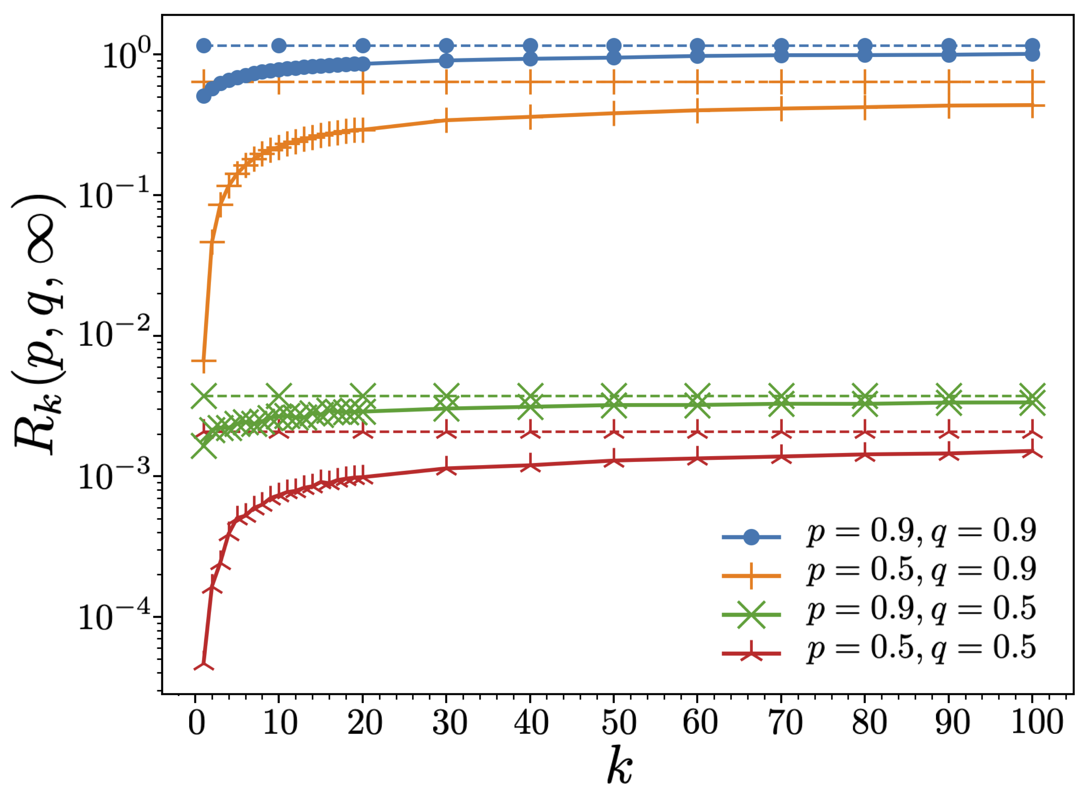
Figure 2: The average rate of the dynamic protocol, indicated by solid lines, approaches the values predicted for $R_{\infty}(p,q,\infty)$. The corresponding bounds are shown above, indicated by dashed lines, for the case that Alice and Bob were both along the diagonal with a hop distance of 10 between them. Low values of $q$ are more detrimental to the rate, as the dynamic routing protocol and time multiplexing can compensate for low $p$ values.

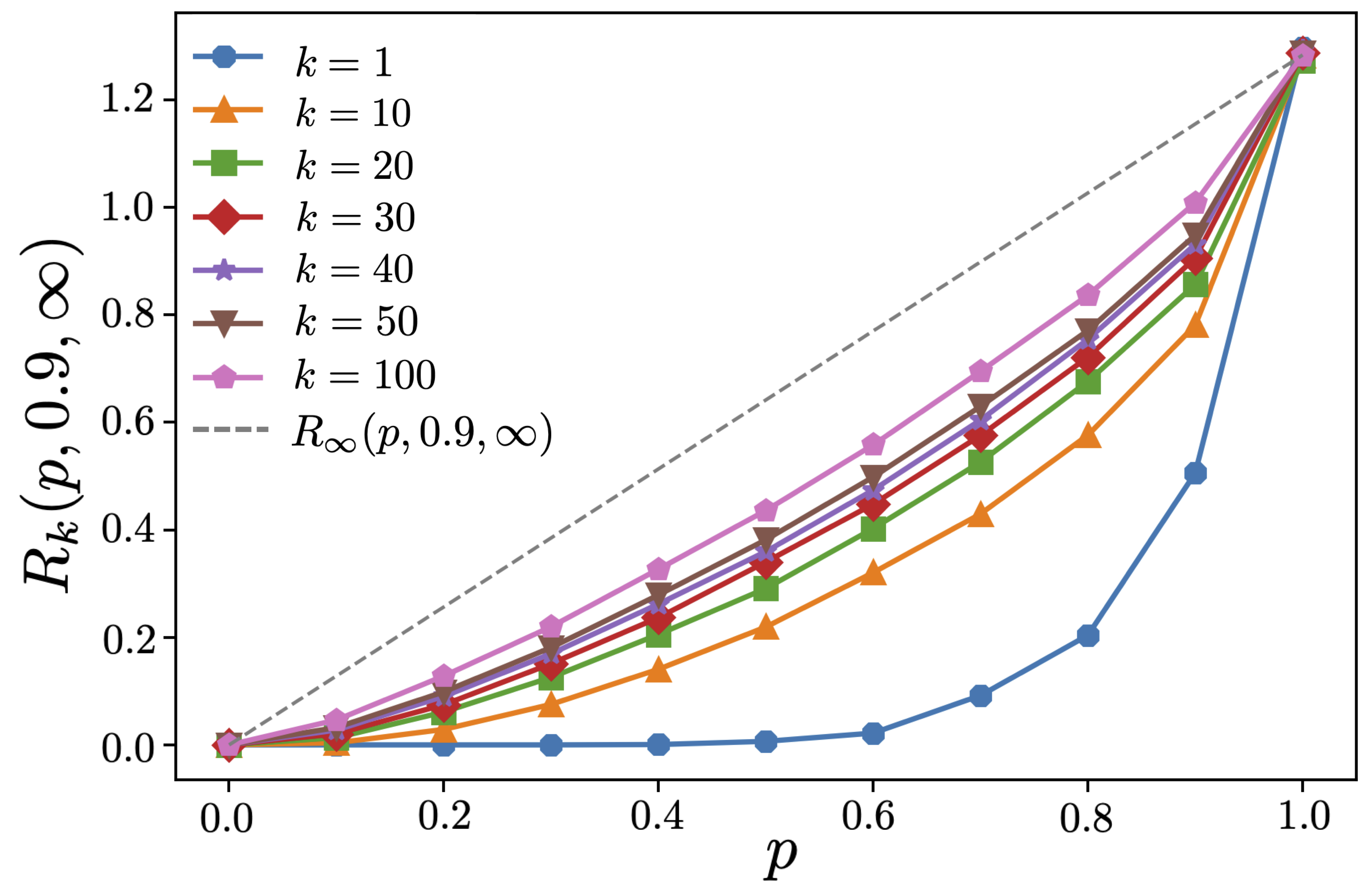
Figure 3: As $k$ increases, the average rate of the dynamic protocol approaches the predicted bound, indicated by the dashed line. As $k\xrightarrow{}\infty$, a linear relationship emerges between the average rate and $p$. The data depicted here is for the case where Alice and Bob were both along the diagonal with a hop distance of 10 between them.

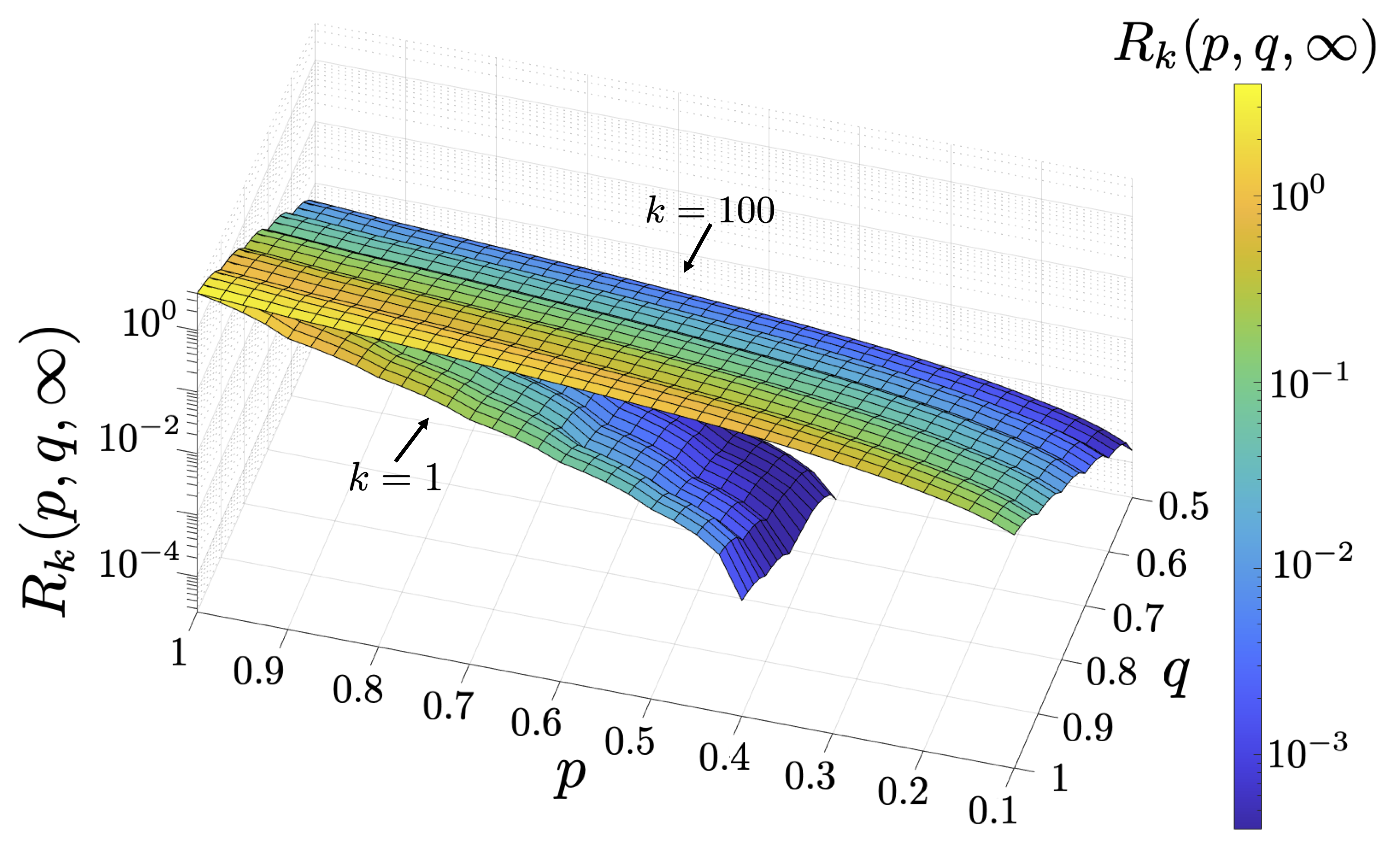
Figure 4: Given that Alice and Bob are both along the diagonal with a hop distance of 10 between them, the average rates for $k=1$ and $k=100$ are compared over different values of $p$ and $q$. Assuming there is no decoherence, increasing the time multiplexing block length can only help the average rate.

.

III-A1 Initial Performance Evaluation

Two consumers placed on a square grid can have at most four edge disjoint paths connecting them. When time multiplexing is introduced so that any edge can have up to $k$ links, the maximum number of connections between consumers is $4k$. If $k$ is sufficiently large, the average number of links along a given edge will be $pk$. Letting $q=1$, we expect $4pk$ connections between consumers. Dividing this by $k$ yields an average rate of $4p$ ebits per time slot. For general $q$, in the limit as $k$ gets large, the highest that the average rate can get is given by

$$R_{\infty}(p,q,\infty)=pR_{1}(1,q,\infty)$$

$$=p\sum_{i=1}^{\theta}q^{m_{i}-1}$$ (3)

where $m_{i}$ is the hop distance of the $i$th shortest path on the underlying graph, which is found via the greedy algorithm.

As depicted in Fig. 2, the dynamic protocol is able to approach this bound on the square grid. We note that low values of $q$ are more detrimental to the rate than low values of $p$. This is because time multiplexing can compensate for low $p$ values. The probability that an edge has at least one successful link after $k$ timesteps is

$$p_{\text{eff}}=1-(1-p)^{k},$$ (4)

which monotonically increases with $k$. If we were to use only one success along any edge, the rate would then be equivalent to $R_{1}(p_{\text{eff}},q,\infty)/k$, which scales as $k^{-1}$. However, this protocol utilizes as much entanglement as possible, ultimately overcoming this scaling. This behavior is further explored in Appendix C. The value of $p$ determines how quickly the average rate approaches $R_{\infty}(p,q,\infty)$, as shown in Fig. 3.

When $p=1$, time multiplexing doesn’t show an improvement to rate since there is no improvement to $p_{\text{eff}}$, as shown in Fig. 4. It is important to note that while the average rate only benefits from larger $k$, the corresponding latency suffers. Therefore realistically, one should choose some finite $k$ based on the desired latency.

III-A2 Varying consumer orientations

The dynamic protocol performs better on the 2D square grid graph when a Euclidean distance metric is used to make swapping decisions, as opposed to a Hop distance metric. However, even with this metric, the dynamic protocol is only able to outperform the static protocol in certain situations.

When $k=1$ and the consumers are oriented along the diagonal, the dynamic protocol outperforms the static protocol for $p<1$. For this specific orientation, the dynamic protocol naturally maps over the same paths as those chosen by the static paths algorithm, unless those links do not exist. However, unlike the static protocol, the dynamic protocol is able to adapt when there are failed links. When $p=1$, the static and dynamic protocols perform equally well. This behavior is consistent regardless of the distance between consumers.

As $k$ increases however, a region emerges in $p,q$ space, shown in Fig. 5, where the static protocol outperforms the dynamic protocol. This behavior stems from the additional ordering that the static path protocol introduces, so that it is able to more efficiently use successful entangled links than the dynamic protocol. The static path protocol does better when $p$ is large, but the exact size and shape of this region depends on $k$ and the distance between consumers. As the distance between consumers grows, the static protocol performs better for lower $p$ values.

When $k=1$ and the consumers are not oriented along the diagonal, there already exists a region in $p,q$ space where $p$ is large where the static protocol outperforms the dynamic protocol. This is because when consumers aren’t along the diagonal, the dynamic protocol doesn’t always choose the most efficient paths. Thus there exists a value $p$ that is large enough that the ability to reroute paths is less useful than the directness of the paths provided by the static path protocol. When $q=1$ the length of a path no longer matters, as all BSMs are deterministic. However, there still exists a range of values of $p$ where the static protocol does better, showing that the dynamic protocol not only chooses longer paths, but also makes decisions that do not result in continuous paths between consumers. As $k$ increases, the quantity $p_{\text{eff}}$ defined in Eqn. (4) increases, explaining why the borders shift to lower $p$ values.

With the condition explained in Appendix B, the dynamic protocol does better for a larger range of values assuming the consumers are along the same column when compared to other off diagonal orientations. When $k>1$ and the Manhattan distance is fixed, the border separating the regions where the dynamic protocol does better from where the static protocol does better occurs at lower $p$ values for the column orientation and higher $p$ values for diagonal orientation. The border for other angles falls between these two cases.

When $k>1$ and the angle is fixed, the border shifts to lower $p$ values as the Manhattan distance is increased. The larger distance between consumers requires more successful BSMs. The ability to reroute is not as important, so static paths do better since they are chosen to minimize the number of these BSMs. As $q$ goes to one however, the difference in path lengths does not matter as much, explaining why the borders appear to tilt diagonally upwards.

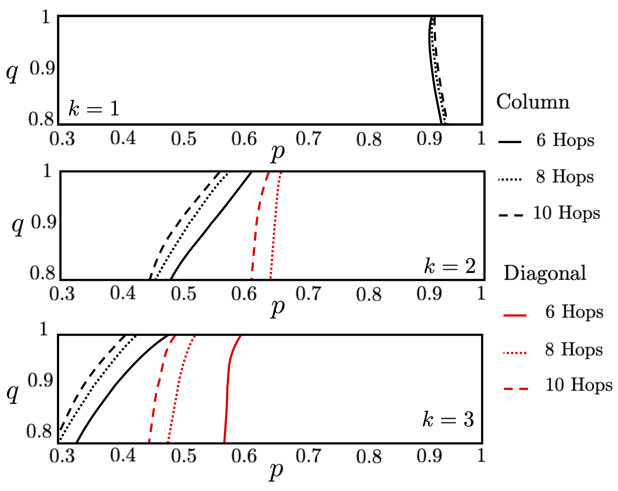
Figure 5: The regions where the dynamic/static protocol performs better for consumers along the column and diagonal with different hop distances apart are demarcated. To the left of the lines the dynamic protocol does better and to the right of the lines the static protocol does better. As $k$ increases, the range of $p$ and $q$ values where the dynamic protocol outperforms the static diminishes. If a line is not shown on the plot, the dynamic protocol does better for all $p,\ q$ values.

III-B Small Network Examples

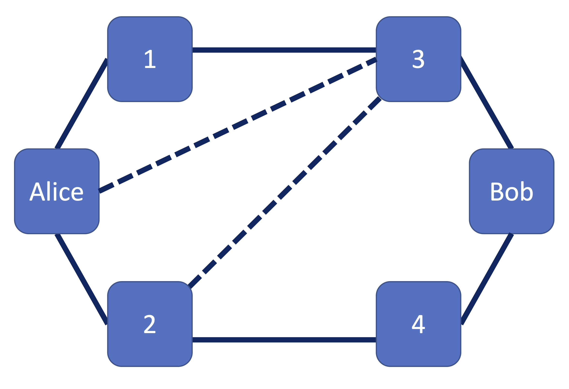
Figure 6: The architecture of our six node graph. The lines depict channels over which links can be generated. The dashed lines are to distinguish the channels between (Alice,3) and (2,3) which may be removed to compare the impact of topology.

Figure 7: The average rates found using a global knowledge (dashed lines) and local link state knowledge (solid lines) are depicted for three variations of the six-node network shown in Fig. 6. Base Graph refers to this network with all channels present. Removal of certain channels of this base graph is shown to always hurt the average rate of the global algoithnm, but can improve the average rate of the local algorithm.

In this section, we evaluate the performance of the protocols on a smaller networks depicted in Fig. 6. This network is meant to be more representative of near-term quantum networks, which will have fewer nodes that span across a building, a campus, or an urban center. The size of the network was also chosen so that the average rate of the dynamic local link state knowledge protocol could be compared against two global link state knowledge routing protocols introduced in [30] and [31].

For the dynamic local link state knowledge protocol, shown in Fig. 7 by the solid lines, the distance metric utilized to inform decisions was based on hop distance. Two different calculations were done to obtain the global link state knowledge rates. Firstly, utilizing the mixed-integer quadratically constrained program (MIQCP) code from [31], which is summarized in Appendix D for convenience, the maximum rate was calculated for every potential snapshot, or unique instance, of the network. The average rate of the network, provided global link state knowledge and optimal decision making, was then calculated by summing over the snapshot rates weighed by their likelihood of occurring. This was then compared against a suboptimal scheme presented in [30]. The main difference was the latter protocol used global link state knowledge and repeatably applied Dijkstra’s algorithm to find the rate of each snapshot. The rates found by this greedy algorithm, which may not be optimal, were similarly weighed by their likelihood, providing the average rate with global link state knowledge and sub-optimal decision-making. The benefit of such a protocol is that the calculation can be performed far more quickly. These results were in agreement up to seven significant digits, and are represented by the dashed lines in Fig. 7.

Three versions of the six node graph shown in Fig. 6 were evaluated. The first included all the channels present in the figure. The second included all, but the channel between repeater 2 and repeater 3. The third included all the channels, but the channel between Alice and repeater 3. The average rates given by the global algorithms did best when more channels were present, since there were simply more potential paths that could be chosen to route over. However, the local protocol did best when the channel between repeaters 2 and 3 was removed. Similar to Braess’ paradox in classical routing, where adding more roads to a road network can slow down the overall traffic, our local algorithm can perform worse on networks when there are more channels if these channels create a contention for paths. Consider a snapshot where all links succeed except for the one between Alice and repeater 3. Since the repeater nodes are making decisions on their own, the local protocol can result in the path given by Alice, 2, 3, Bob, which intersects the two otherwise disjoint paths. The local protocol performs best on architectures where there are multiple subsections of the graph connected in parallel at the consumer nodes. Otherwise, it might serve useful to pre-establish an additional network-division similar to that introduced in [22] to work around this.

IV Memories with limited storage lifetime

The previously discussed results imply that as long as consumers are willing to wait for some increased latency cost, time multiplexing always helps improve the rate of entanglement distribution. However, as time multiplexing blocks increase in length, qubits stored in the quantum memories experience more decoherence. We now relax the assumption that qubits are held in the quantum memories indefinitely and instead will evaluate for a finite valued $\mu$. This model will be applied to a 2D grid network to show that for given network conditions, there arises a finite $k$ for which the rate of entanglement is maximized.

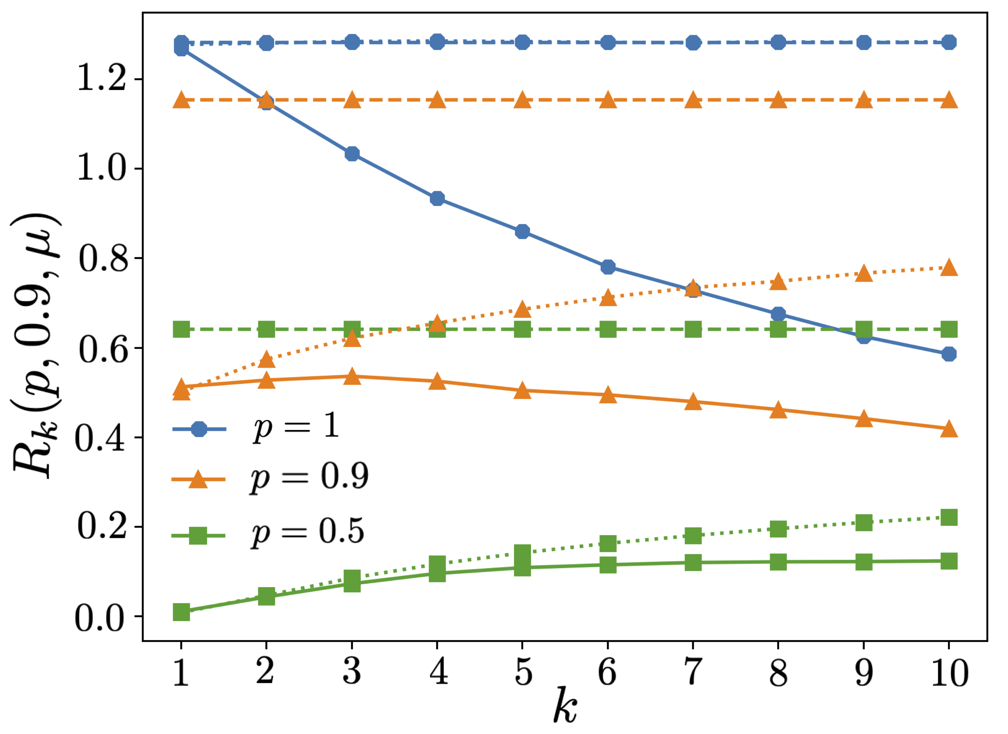
Figure 8: The average rates for a variety of $(p,q)$ values are shown here in the presence and absence of decoherence. The solid line is for $\mu=100$, the dotted line is for $\mu=\infty$ and the dashed line shows the upper limit $R_{\infty}(p,q,\infty)$. In the case of $p=1$, the dotted and dashed lines overlap.

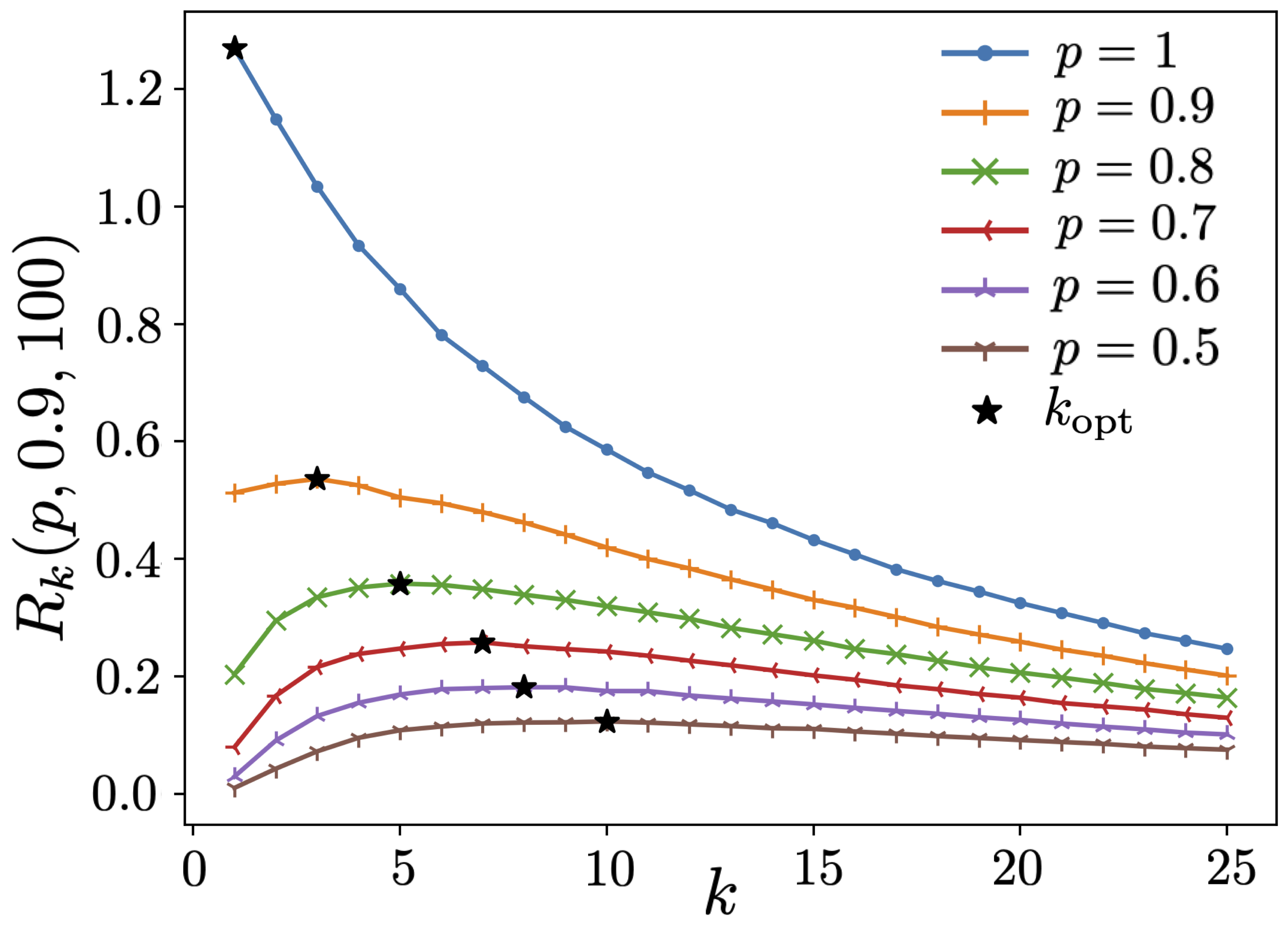
Figure 9: In the presence of decoherence, each value of $p$ has an optimal value $k$, denoted as $k_{\text{opt}}$, such that the average rate is largest for that time multiplexing block length. As $p$ decreases, $k_{\text{opt}}$ increases.

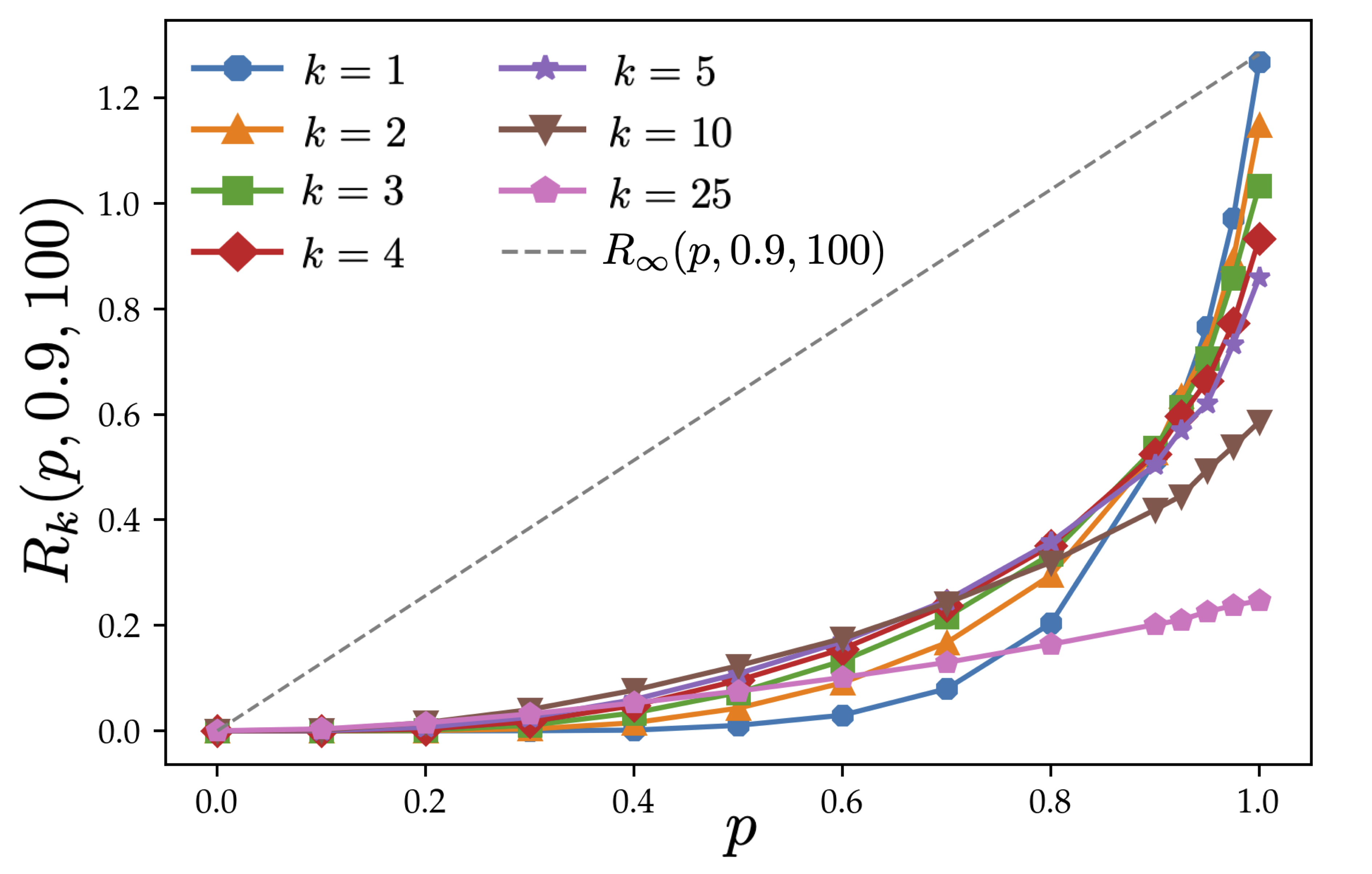
Figure 10: In the presence of decoherence, time multiplexing can help bridge the gap between $R_{1}(p,q,100)$ and $R_{\infty}(p,q,\infty)$. However, this improvement is bounded by an envelope determined by the value of $\mu$.

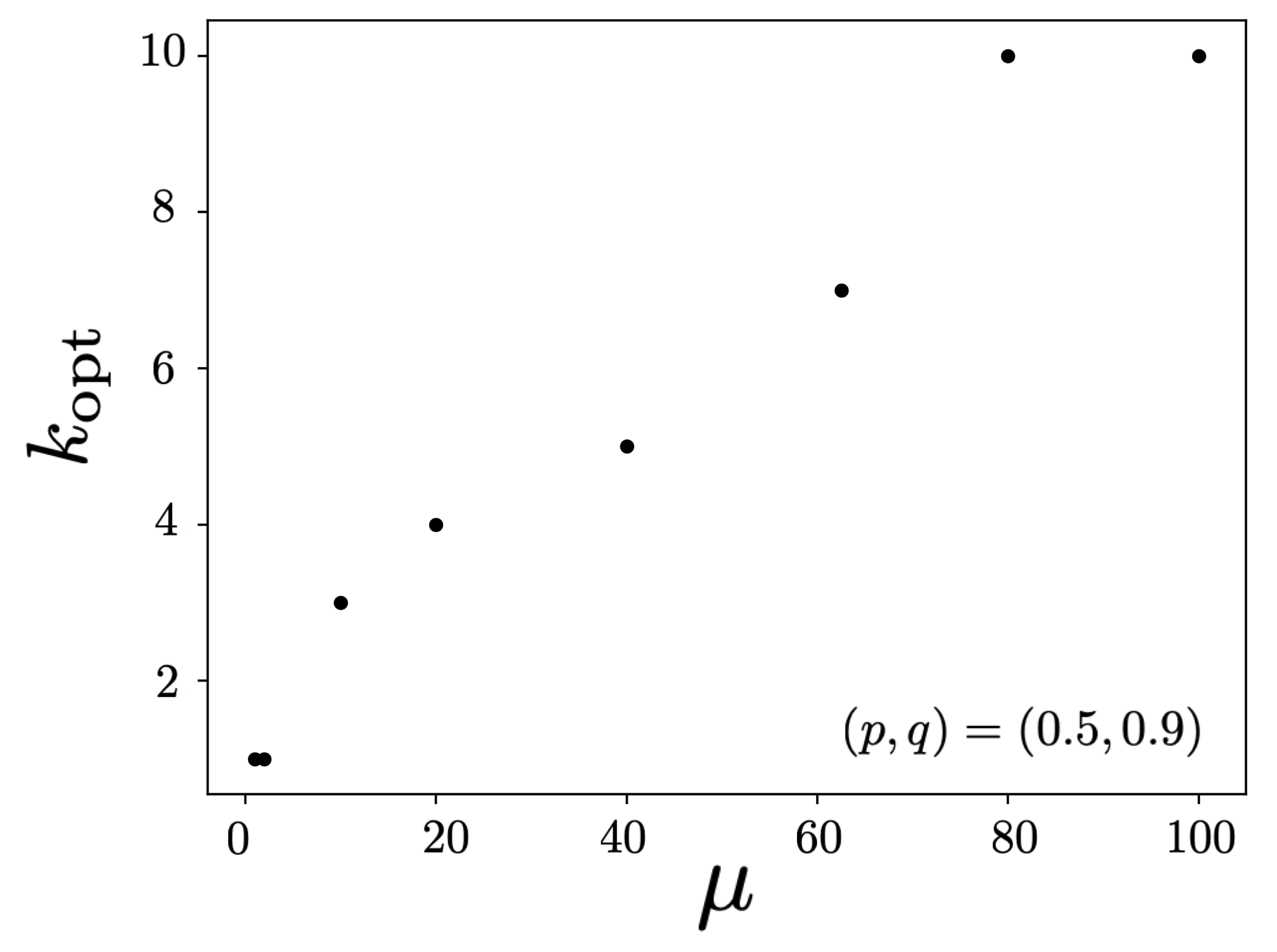
Figure 11: There is a monotonically increasing relationship between $k_{\text{opt}}$ and $\mu$, which in the limit of $\mu\xrightarrow{}\infty$ agrees with the results without decoherence. Note, $k=10$ was the maximum value tried for $k$.

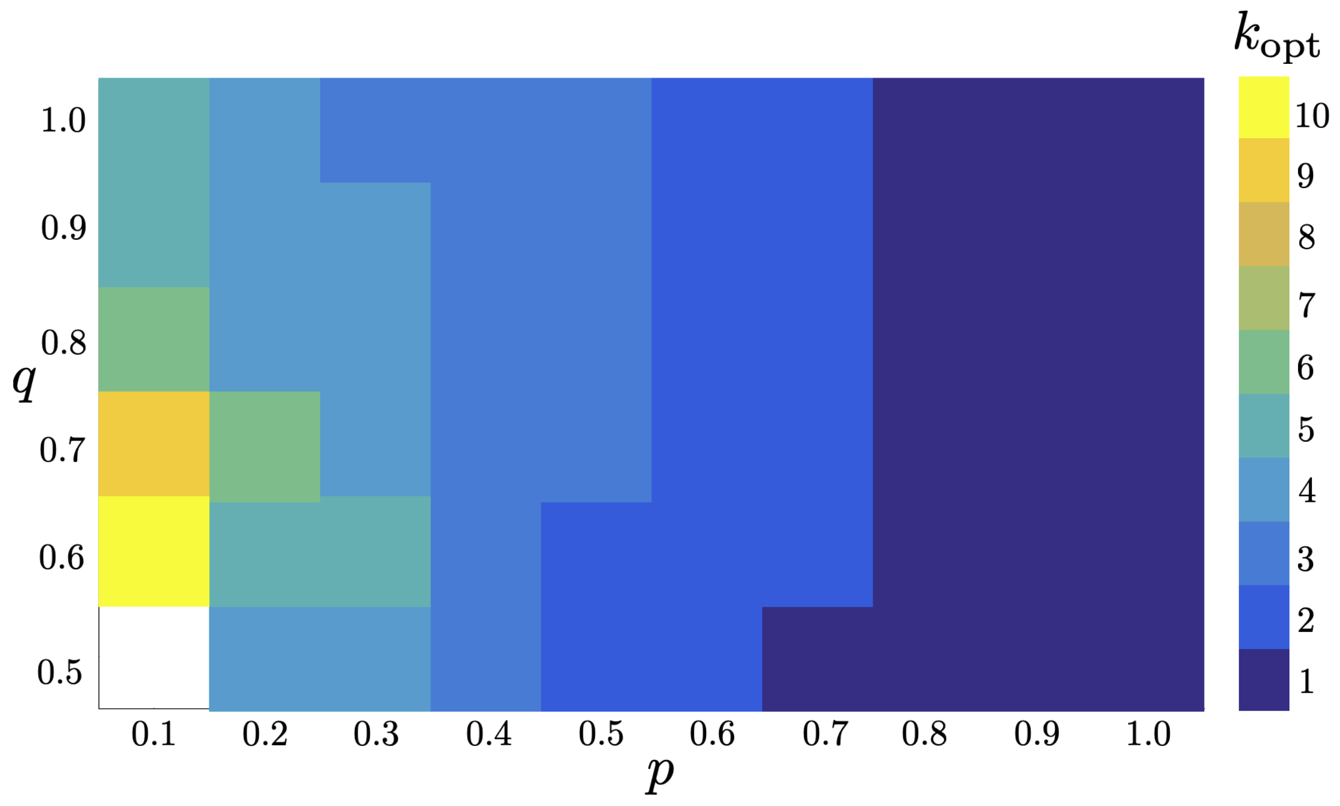
Figure 12: The value of $k_{\text{opt}}\in[1,10]$ is indicated here for a range of values of $p$ and $q$. No optimal k was found in the white region, as the rate remained zero over all trials.

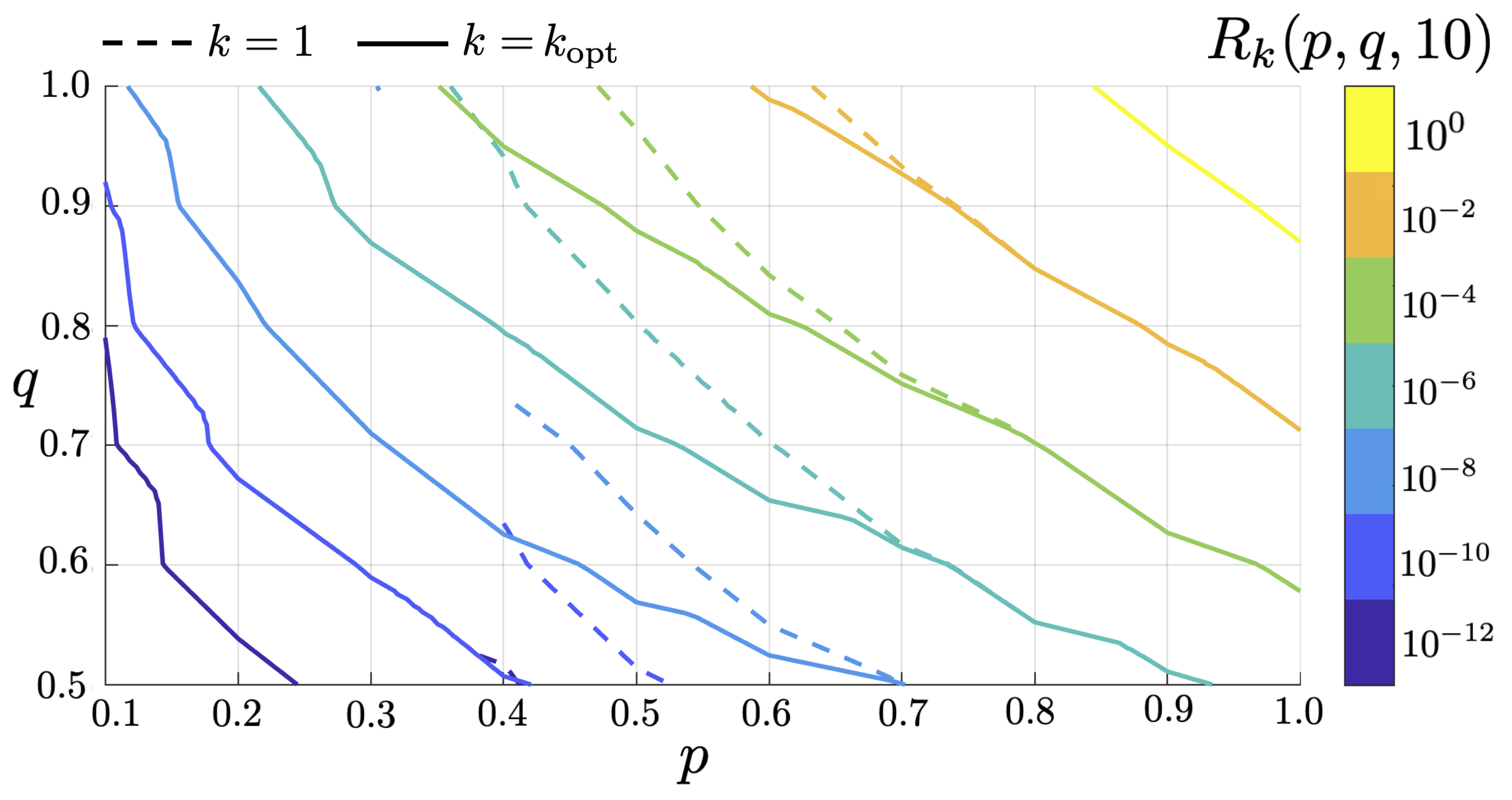
Figure 13: The solid lines here indicate the contour lines of $R_{k_{\text{opt}}}(p,q,10)$ whereas the dashed lines demarcate the contour lines of $R_{1}(p,q,10)$. Note the dashes lines do not span the entire space, because due to the finite number of trials run, they returned rates of zero below $p=0.4$.

For such a network, there exists a trade-off between the benefits of increased time multiplexing block length and the risk of losing already established entangled links, as shown in Fig. 8. This relationship results in an optimal time multiplexing value, $k_{\text{opt}}$, dependent on the network conditions. Fig. 9 shows that as $p$ decreases, $k_{\text{opt}}$ increases. When $p$ goes to one, so that external links are deterministic, time multiplexing is no longer useful, and $k_{\text{opt}}=1$. Fig. 10 shows that even with decoherence, there is an improvement in rate with time multiplexing, as seen by the envelope. The amount of improvement is limited by the magnitude of $\mu$. As $\mu$ goes to infinity, the achievable rates with time multiplexing will increase, eventually resembling Fig. 3. Fig. 11 also agrees with previous results, as it shows that as $\mu$ increases, so does $k_{\text{opt}}$. In the case where quantum memories have infinite lifetime, and thus no decoherence, the rate continues to increase with $k$. Fig. 13 shows the improved rate over $(p,q)$ space, using the values of $k_{\text{opt}}$ shown in Fig. 12. There is noise in the data stemming from the finite number of trials the Monte Carlo simulation was run over and the limited data points collected, so it is not immediately clear if the value of $q$ impacts the optimal $k$, despite it clearly affecting the average rate. However, it is once again clear that time multiplexing helps, especially in the case of lower $p$.

V Conclusion

This study discusses a local link state knowledge multi-path routing protocol that utilizes time multiplexed repeaters. In the case of no decoherence, the average entanglement rate increases monotonically with the time multiplexing block length $k$, and approaches the upper bound given by Eqn. (III-A1). This is because the value of the effective $p$, $p_{\text{eff}}$, increases with $k$. Theoretically, to maximize the rate of entanglement distribution, it is best to let $k\xrightarrow{}\infty$. This is not practical, however, as latency and the required number of quantum memories also become infinite. Therefore, the value of $k$ must be chosen while keeping both the initial latency and memory buffer length in mind. Future work should consider the effects that memory buffer length may have on optimal scheduling.

The distance metric chosen, and the topology of the network itself, impacts how effectively the dynamic protocol performs. For the case of a 2D grid, the dynamic protocol performs best when consumers reside on the diagonal. In general, the performance of the dynamic protocol when compared to the static protocol depends on the values of $p,q,k$ and the locations of the consumers. The dynamic protocol was also applied to a smaller six node network, so that it could be compared to the global optimum rate. The local link state knowledge protocol can perform comparably well when consumers are connected via disjoint subsets of repeaters. However, when there is a high contention for the same paths, our local protocol cannot approach the average rates seen with global link state knowledge. Future works could evaluate wider variety of topologies to further explore how the structure of the quantum network impacts the performance of the protocol.

A step function decoherence model was also used in the simulation to see how the mean lifetime of qubits held in the quantum memories impacted the effects of time multiplexing. In this case, an optimal $k$ value emerges which balances the benefits from time multiplexing with the increased risk of losing a Bell pair. It was seen that as $p$ decreases or $\mu$ increases, the value of $k_{\text{opt}}$ increases. To fully understand the effect of $q$ on $k_{opt}$, further study is needed; however, we conjecture that there may be a connection stemming from the fact increasing $k$ allows for more direct paths to be routed over. Overall, the results with decoherence agree with the results without decoherence when $\mu\xrightarrow{}\infty$.

The decoherence model used in this paper can be improved upon by introducing non-unit fidelity links. These links could then undergo depolarization noise channels to model both the effects of being held in the quantum memory over time, as well as the noise introduced by the imperfect gates used to perform BSMs. With this, time multiplexing could then be combined with distillation techniques, which would result in purer states, but at the cost of reducing to the number of Bell pairs delivered to the consumers over some fixed time. A protocol dictating how and when to distill links would then need to be considered.

Appendix A Distance-Based Protocol Pseudocode

for each edge, $e$, in the network topology do $\triangleright$ external phase

     $r_{1}\leftarrow\text{source}(e)$

     $r_{2}\leftarrow\text{target}(e)$

     $\text{qubits}[r_{1},r_{2}]\leftarrow\text{LIST()}$

     $\text{qubits}[r_{2},r_{1}]\leftarrow\text{LIST()}$

     for each timestep, $t$, from 1 to $k$ do

         if $\text{unif\_rand}(0.0,1.0)<p$ then $\triangleright$ link success

              $q_{1}\leftarrow\text{ an unentangled qubit from }r_{1}$

              $q_{2}\leftarrow\text{ an unentangled qubit from }r_{2}$

              $\text{entangle}(q_{1},q_{2})$

              if $\text{exp\_rand}(1.0/\mu)>=k-t$ then

                  $\text{append}(q_{1},\text{qubits}[r_{1},r_{2}])$

              else

                  $\text{decohere}(q_{1})$

              end if

              if $\text{exp\_rand}(1.0/\mu)>=k-t$ then

                  $\text{append}(q_{2},\text{qubits}[r_{2},r_{1}])$

              else

                  $\text{decohere}(q_{2})$

              end if

         end if

     end for

end for

for each repeater, r, in the network do $\triangleright$ internal phase

     while $\text{qubits}[r,\ldots]\text{ contains at least two values}$ do

         $v\leftarrow\text{closest neighbor to Alice entangled with }r$

         $w\leftarrow\text{closest neighbor to Bob entangled with }r$

         if $v\text{ is not }w$ then

              $q_{1}\leftarrow\text{pop}(\text{qubits}[r,v])$

              $q_{2}\leftarrow\text{pop}(\text{qubits}[r,w])$

         else if $\exists\text{ a neighbor}\neq v\text{ entangled with }r$ then

              $v^{\prime}\leftarrow\text{second closest neighbor to Alice entangled with }r$

              $w^{\prime}\leftarrow\text{second closest neighbor to Bob entangled with }r$

              if $d_{A_{v^{\prime}}}+d_{B_{w}}<d_{A_{v}}+d_{B_{w}^{\prime}}$ then

                  $q_{1}\leftarrow\text{pop}(\text{qubits}[r,v^{\prime}])$

                  $q_{2}\leftarrow\text{pop}(\text{qubits}[r,w])$

              else if $d_{A_{v^{\prime}}}+d_{B_{w}}>d_{A_{v}}+d_{B_{w}^{\prime}}$ then

                  $q_{1}\leftarrow\text{pop}(\text{qubits}[r,v])$

                  $q_{2}\leftarrow\text{pop}(\text{qubits}[r,w^{\prime}])$

              else if $d_{B_{v^{\prime}}}+d_{A_{w}}>d_{B_{v}}+d_{A_{w}^{\prime}}$ then

                  $q_{1}\leftarrow\text{pop}(\text{qubits}[r,v^{\prime}])$

                  $q_{2}\leftarrow\text{pop}(\text{qubits}[r,w])$

              else

                  $q_{1}\leftarrow\text{pop}(\text{qubits}[r,v])$

                  $q_{2}\leftarrow\text{pop}(\text{qubits}[r,w^{\prime}])$

              end if

         else

              $q_{1}\leftarrow\text{pop}(\text{qubits}[r,v])$

              $q_{2}\leftarrow\text{pop}(\text{qubits}[r,w])$

         end if

         $\text{BSM}(q_{1},q_{2})$

     end while

end for

Appendix B “Straight Path” Heuristic

Recall the Distance Based Routing Protocol definition given in Section II.

At every node the successfully connected neighbor closest to Alice/Bob was denoted $v/w$, and their relative distances were defined $d_{Av}/d_{Bw}$. When $v$ and $w$ referred to the same neighbor node, initially new neighbors $v^{\prime}$, the second closest neighbor to Alice, and $w^{\prime}$, the second closest neighbor to Bob, were found. The quantity $d_{Av^{\prime}}+d_{Bw}$ and $d_{Av}+d_{Bw^{\prime}}$ would then be compared, and the pair that minimizes this choice will be chosen to perform a swap.

If these quantities were equal, the “straight path” heuristic was evaluated. The quantities $d_{Bv^{\prime}}+d_{Aw}$ and $d_{Bv}+d_{Aw^{\prime}}$ would be compared, and the pair that maximizes this value would be chosen to perform a swap.

Prior to this addition, the average rate of the distance based routing protocol was considerably lower when consumers were off diagonal for the 2D grid graph. An example of a snapshot generated prior to the introduction of the straight path heuristic is shown in Fig. 14, which is clearly not routing along the most direct paths, despite attaining the maximum rate of 4. However, repeater nodes 2, 13, 15, 19, 21, and 32 all could make different decisions, such that the rate of a given snapshot, even when $p=1,q=1$, is as low as 1. After the inclusion of this “straight path” heuristic, all snapshots gave a rate of three or four when $p=1,q=1$. Consumers on the diagonal of the 2D graph, as well as consumers in the small networks discussed here, did just as well with this condition as without it.

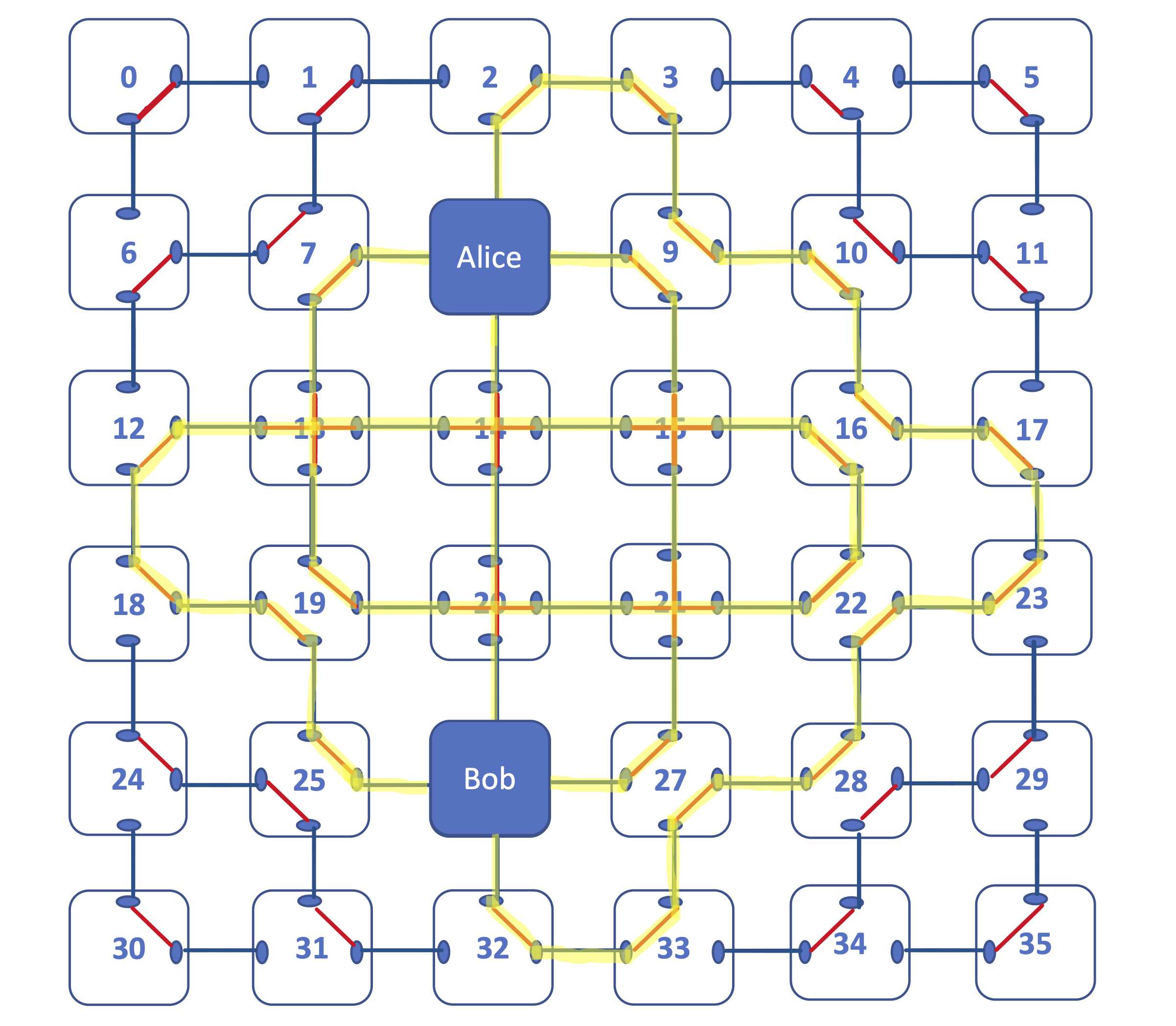
Figure 14: A possible snapshot for $p=1,q=1,k=1$ on a small 2D grid graph when the straight path preference is not included.

Appendix C Utilizing Multiple Successes along Edges

The probability that an edge has at least one successful link after $k$ timesteps is given by Eqn. (4) If the local protocol proposed in this paper was limited to using only one success along any edge, the rate would then be equivalent to $R_{1}(p_{\text{eff},q,\infty})/k$, which scales as $k^{-1}$. This scaling is overcome by the local link state protocol which is configured to use as much entanglement as possible. Ideally using multiple successes along edges would always result in higher rates than limiting the protocol to one success. However, in the regime of low $k$ values, there are cases where the opposite is true as shown in Fig. 15. In this figure, using multiple successes actually reduces the average rate for $k\in[2,6]$. This is because when multiple successes are introduced, there is increased likelihood for self loops to be made. This example is also for two consumers in a 2D grid network, which has high connectivity and increased likelihood for self loops when compared to the smaller networks evaluated. The smaller networks did not show this behavior.

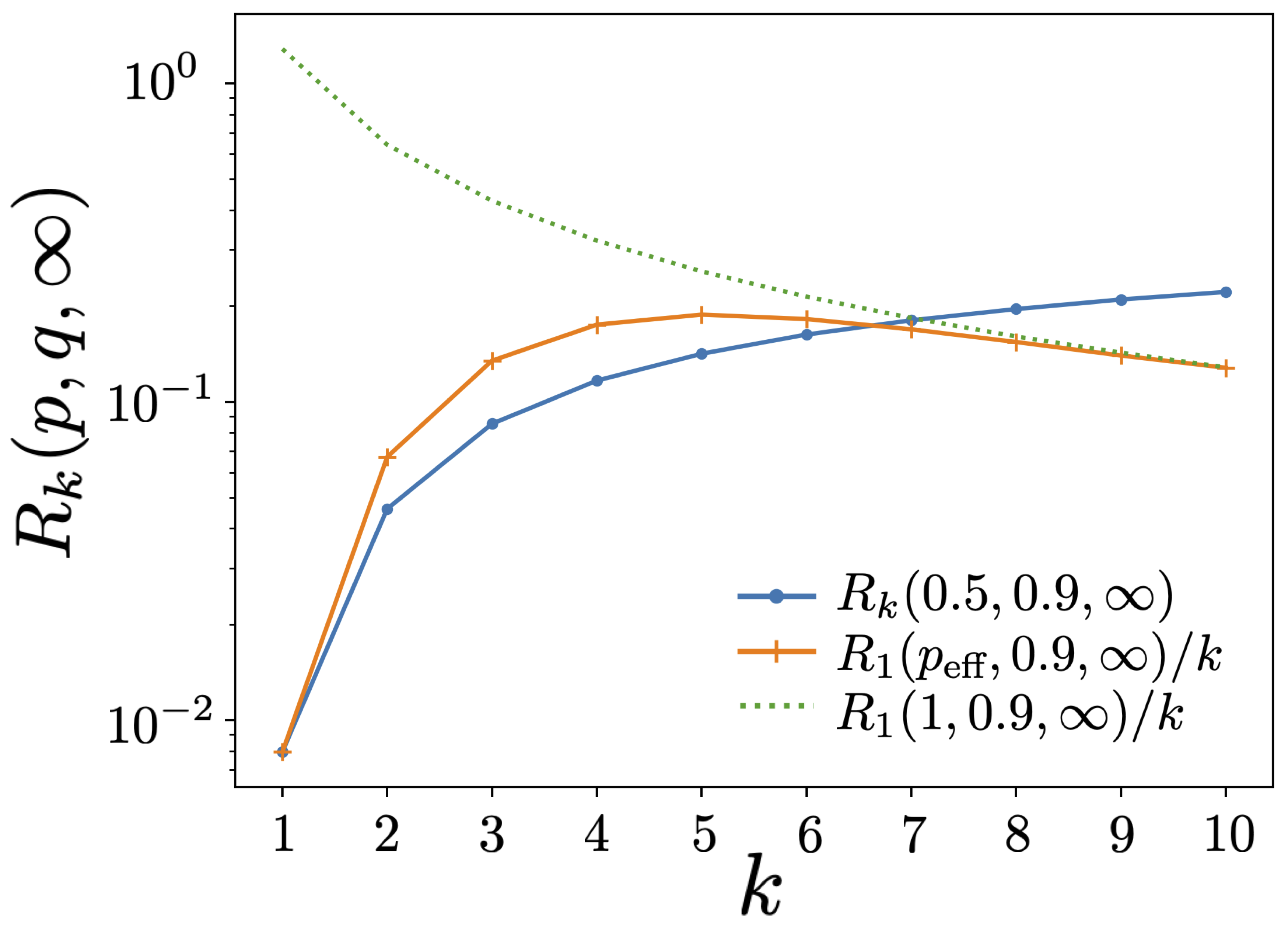
Figure 15: Comparison of the average rate achievable with time multiplexing when using only one success per edge, denoted $R_{1}(p_{\text{eff}},0.9,\infty)/k$ , vs using multiple successes across timesteps, shown by $R_{k}(0.5,0.9,\infty)/k$. An upper bound is given by $R_{1}(1,0.9,\infty)/k$ in order to highlight the inverse scaling with $k$. Data was collected from a 2D square grid where Alice and Bob were 10 hops away apart and on the diagonal.

Appendix D Maximal Bipartite Entanglement Capacity MIQCP psuedocode

A brief explanation of the MIQCP calculations is provided here, but further details can be found in [31]. Assume initially that $k=1$. First, the individual capacities of all possible snapshots of the network are found. These are weighted by their probability of occurrence and summed over, giving the average capacity of the network. The formulation to find the individual capacities of the snapshots is given below.

Let $s$ and $t$ be the two consumer nodes, and $E$ be the set of edges present on the snapshot. Let $F_{ij}$, $i\neq s$, $j\neq t$, represent flow from node $i$ to $j$. The objective function and the set of constraints are:

$$\max\sum\limits_{(j,t)\in E}F_{jt}$$ (5)

$$0\leq F_{ij}\leq 1,\quad\forall(i,j)\in E,$$ (6)

$$x_{ijk}\in\{0,1\},\quad\forall(i,j),~{}(j,k)\in E~{}/\ i\neq k,~{}j\neq s,t,$$ (7)

$$\sum\limits_{k}(x_{ijk}+x_{kji})\leq 1\quad\forall(i,j)\in E,$$ (8)

$$x_{ijk}(F_{ij}q_{j}-F_{jk})=0,\quad\forall(i,j),(j,k)\in E,$$ (9)

$$\sum\limits_{k}x_{ijk}\geq F_{ij},\quad\forall(i,j)\in E~{}/j\neq t,$$ (10)

$$\sum\limits_{j\in V}(F_{ij}-F_{ji}q_{i})=0,\quad\forall i\in V,~{}i\neq s,t.$$ (11)

If $k>1$, the same MIQCP may be used as long as the representation of network evaluated is first transformed. To do this, each edge is transformed into two edges and a new node with $q=1$, so that $(i,j)$ becomes $(i,n)$ and $(n,j)$.

Appendix E Rate equation for deterministic link generation, but memory decoherence

In this section it is shown how to analytically calculate the average flow of entanglement between consumers for the case $p=1$ and $\mu\in\mathbb{R}_{>0}$ along a path of fixed length $d$. This can then be used to compare against our simulated $R_{k}(1,q,\mu)$ values.

In the presence of imperfect memories, let the random variable describing the lifetime of an individual link be labelled $L$. This value is sampled from

$$p_{L}[l]=\frac{1}{\mu}e^{\frac{-l}{\mu}},$$ (12)

where $l\in\mathbb{R}_{\geq 0}$. The actual quantity of interest is the probability that the lifetime of a link is greater than some value $l$, which is given by:

$$p_{L}[L\geq l]=e^{\frac{-l}{\mu}}.$$ (13)

A link generated in the $i$th time slot, where $i\in[1,k]$, must survive until the $k$th time slot in order to be used to connect two consumers. Therefore the likelihood of it having a lifetime at least $t=k-i$ timesteps long is given by:

$$s(t)=p_{L}[L\geq t]=e^{\frac{-t}{\mu}}$$

which is denoted $s(t)$ for brevity.

Note for the most recently generated link, i.e. when $i=k$ and $t=0$, $s(t=0)=1$. Since every edge will have such a link in the case $p=1$, there will always be at least one path along the chain of repeaters over which $d-1$ BSMs will be performed to connect consumers. This case will then contribute the term $\frac{q^{d-1}}{k}$ to the final rate calculation. From here forward then the focus will be on links where $i,t\in[1,k-1]$.

The probability that any edge has $n$ correctable links generated in time slots $i\in[1,k-1]$ at the end of the $k$ timesteps is:

$$p_{N}[n]=\sum_{\begin{subarray}{c}x_{1},..x_{n}\in[1,k-1]\\ x_{1}\neq\cdots\neq x_{n}\end{subarray}}^{k-1}\prod_{i\in[x_{1},..x_{n}]}\prod_{j\notin[x_{1},..x_{n}]}s(i)(1-s(j))$$

The probability of having $m$ paths then comes from $M=min(N_{1},N_{2},\cdots,N_{d})$ where $N_{i}$ are iid from $p_{N}[n]$. The probability of having $m$ paths is then given by:

$$p_{M}[m]=\sum_{x=0}^{d-1}\frac{d!}{d!(d-x)!}p_{N}[m]^{d-x}\sum_{i_{1},...i_{x}=m+1}^{k-1}\prod_{j\in[i_{1},...i_{x}]}p_{N}[j]$$

The average rate attainable by a linear chain of time multiplexed repeaters of length $d$ block length $k$ when $p=1$ is then given by:

$$R_{k}(1,q,\mu)=\frac{q^{d-1}}{k}\big{(}1+\sum_{m=1}^{k-1}mp_{M}(m)\big{)}$$ (15)

with $p_{M}(m)$ defined above.

References

- [1] A. K. Ekert, Quantum Cryptography and Bell’s Theorem. Boston, MA: Springer US, 1992, pp. 413–418.
- [2] C. H. Bennett, G. Brassard, and N. D. Mermin, “Quantum cryptography without Bell’s theorem,” Physical Review Letters, vol. 68, no. 5, pp. 557–559, Feb. 1992. [Online]. Available: https://link.aps.org/doi/10.1103/PhysRevLett.68.557
- [3] Y. Xia, W. Li, W. Clark, D. Hart, Q. Zhuang, and Z. Zhang, “Demonstration of a Reconfigurable Entangled Radio-Frequency Photonic Sensor Network,” Physical Review Letters, vol. 124, no. 15, p. 150502, Apr. 2020. [Online]. Available: https://link.aps.org/doi/10.1103/PhysRevLett.124.150502
- [4] M. R. Grace, C. N. Gagatsos, and S. Guha, “Entanglement-enhanced estimation of a parameter embedded in multiple phases,” Phys. Rev. Res., vol. 3, p. 033114, Aug 2021. [Online]. Available: https://link.aps.org/doi/10.1103/PhysRevResearch.3.033114
- [5] P. C. Humphreys, M. Barbieri, A. Datta, and I. A. Walmsley, “Quantum enhanced multiple phase estimation,” Phys. Rev. Lett., vol. 111, p. 070403, Aug 2013. [Online]. Available: https://link.aps.org/doi/10.1103/PhysRevLett.111.070403
- [6] T. J. Proctor, P. A. Knott, and J. A. Dunningham, “Multiparameter Estimation in Networked Quantum Sensors,” Physical Review Letters, vol. 120, no. 8, p. 080501, Feb. 2018. [Online]. Available: https://link.aps.org/doi/10.1103/PhysRevLett.120.080501
- [7] Q. Zhuang, Z. Zhang, and J. H. Shapiro, “Distributed quantum sensing using continuous-variable multipartite entanglement,” Physical Review A, vol. 97, no. 3, p. 032329, Mar. 2018. [Online]. Available: https://link.aps.org/doi/10.1103/PhysRevA.97.032329
- [8] R. Van Meter and S. J. Devitt, “The Path to Scalable Distributed Quantum Computing,” Computer, vol. 49, no. 9, pp. 31–42, Sep. 2016, conference Name: Computer.
- [9] S. Pirandola, R. Laurenza, C. Ottaviani, and L. Banchi, “Fundamental limits of repeaterless quantum communications,” Nature Communications, vol. 8, no. 1, p. 15043, Apr. 2017. [Online]. Available: https://www.nature.com/articles/ncomms15043
- [10] M. Takeoka, S. Guha, and M. M. Wilde, “Fundamental rate-loss tradeoff for optical quantum key distribution,” Nature Communications, vol. 5, no. 1, pp. 1–7, Oct. 2014, number: 1 Publisher: Nature Publishing Group. [Online]. Available: https://www.nature.com/articles/ncomms6235
- [11] S. Guha, H. Krovi, C. A. Fuchs, Z. Dutton, J. A. Slater, C. Simon, and W. Tittel, “Rate-loss analysis of an efficient quantum repeater architecture,” Physical Review A, vol. 92, no. 2, p. 022357, Aug. 2015. [Online]. Available: https://link.aps.org/doi/10.1103/PhysRevA.92.022357
- [12] M. Pant, H. Krovi, D. Englund, and S. Guha, “Rate-distance tradeoff and resource costs for all-optical quantum repeaters,” Physical Review A, vol. 95, no. 1, p. 012304, Jan. 2017. [Online]. Available: https://link.aps.org/doi/10.1103/PhysRevA.95.012304
- [13] L.-M. Duan, M. D. Lukin, J. I. Cirac, and P. Zoller, “Long-distance quantum communication with atomic ensembles and linear optics,” Nature, vol. 414, no. 6862, pp. 413–418, Nov. 2001. [Online]. Available: https://doi.org/10.1038/35106500
- [14] Y. Lee, E. Bersin, A. Dahlberg, S. Wehner, and D. Englund, “A quantum router architecture for high-fidelity entanglement flows in quantum networks,” npj Quantum Information, vol. 8, no. 1, pp. 1–8, Jun. 2022, number: 1 Publisher: Nature Publishing Group. [Online]. Available: https://www.nature.com/articles/s41534-022-00582-8
- [15] E. Schoute, L. Mancinska, T. Islam, I. Kerenidis, and S. Wehner, “Shortcuts to quantum network routing,” Oct. 2016, arXiv:1610.05238 [quant-ph]. [Online]. Available: http://arxiv.org/abs/1610.05238
- [16] K. Chakraborty, F. Rozpedek, A. Dahlberg, and S. Wehner, “Distributed Routing in a Quantum Internet,” Jul. 2019, arXiv:1907.11630 [quant-ph]. [Online]. Available: http://arxiv.org/abs/1907.11630
- [17] M. Pant, H. Krovi, D. Towsley, L. Tassiulas, L. Jiang, P. Basu, D. Englund, and S. Guha, “Routing entanglement in the quantum internet,” npj Quantum Information, vol. 5, no. 1, pp. 1–9, Mar. 2019, number: 1 Publisher: Nature Publishing Group. [Online]. Available: https://www.nature.com/articles/s41534-019-0139-x
- [18] T. N. Nguyen, K. J. Ambarani, L. Le, I. Djordjevic, and Z.-L. Zhang, “A Multiple-Entanglement Routing Framework for Quantum Networks,” Jul. 2022, arXiv:2207.11817 [cs]. [Online]. Available: http://arxiv.org/abs/2207.11817
- [19] L. Zhang, S.-X. Ye, Q. Liu, and H. Chen, “Multipath concurrent entanglement routing in quantum networks based on virtual circuit,” in 2022 4th International Conference on Advances in Computer Technology, Information Science and Communications (CTISC), Apr. 2022, pp. 1–5.
- [20] C. Li, T. Li, Y.-X. Liu, and P. Cappellaro, “Effective routing design for remote entanglement generation on quantum networks,” npj Quantum Information, vol. 7, no. 1, pp. 1–12, Jan. 2021, number: 1 Publisher: Nature Publishing Group. [Online]. Available: https://www.nature.com/articles/s41534-020-00344-4
- [21] M. Victora, S. Krastanov, A. S. de la Cerda, S. Willis, and P. Narang, “Purification and Entanglement Routing on Quantum Networks,” Nov. 2020, arXiv:2011.11644 [quant-ph]. [Online]. Available: http://arxiv.org/abs/2011.11644
- [22] A. Patil, M. Pant, D. Englund, D. Towsley, and S. Guha, “Entanglement generation in a quantum network at distance-independent rate,” npj Quantum Information, vol. 8, no. 1, p. 51, May 2022. [Online]. Available: https://www.nature.com/articles/s41534-022-00536-0
- [23] E. Sutcliffe and A. Beghelli, “Multi-user entanglement distribution in quantum networks using multipath routing,” 2023.
- [24] L. Gyongyosi and S. Imre, “Decentralized base-graph routing for the quantum internet,” Physical Review A, vol. 98, no. 2, p. 022310, Aug. 2018, publisher: American Physical Society. [Online]. Available: https://link.aps.org/doi/10.1103/PhysRevA.98.022310
- [25] P. Dhara, A. Patil, H. Krovi, and S. Guha, “Subexponential rate versus distance with time-multiplexed quantum repeaters,” Physical Review A, vol. 104, no. 5, p. 052612, Nov. 2021. [Online]. Available: https://link.aps.org/doi/10.1103/PhysRevA.104.052612
- [26] A. Patil, J. Jacobson, E. Van Milligen, D. Towsley, and S. Guha, “Distance-independent entanglement generation in a quantum network using space-time multiplexed Greenberger–Horne–Zeilinger (GHZ) measurements,” in 2021 IEEE International Conference on Quantum Computing and Engineering (QCE). IEEE, oct 2021.
- [27] P. Nain, G. Vardoyan, S. Guha, and D. Towsley, “On the Analysis of a Multipartite Entanglement Distribution Switch,” Proceedings of the ACM on Measurement and Analysis of Computing Systems, vol. 4, no. 2, pp. 1–39, Jun. 2020. [Online]. Available: https://dl.acm.org/doi/10.1145/3392141
- [28] G. Vardoyan, S. Guha, P. Nain, and D. Towsley, “On the Stochastic Analysis of a Quantum Entanglement Switch,” ACM SIGMETRICS Performance Evaluation Review, vol. 47, no. 2, pp. 27–29, Dec. 2019. [Online]. Available: https://dl.acm.org/doi/10.1145/3374888.3374899
- [29] P. Wang, C.-Y. Luan, M. Qiao, M. Um, J. Zhang, Y. Wang, X. Yuan, M. Gu, J. Zhang, and K. Kim, “Single ion qubit with estimated coherence time exceeding one hour,” Nature Communications, vol. 12, no. 1, p. 233, Jan. 2021, number: 1 Publisher: Nature Publishing Group. [Online]. Available: https://www.nature.com/articles/s41467-020-20330-w
- [30] M. Pant, H. Krovi, D. Towsley, L. Tassiulas, L. Jiang, P. Basu, D. Englund, and S. Guha, “Routing entanglement in the quantum internet,” npj Quantum Information, vol. 5, no. 1, p. 25, 2019. [Online]. Available: https://doi.org/10.1038/s41534-019-0139-x
- [31] G. Vardonyan, E. Van Milligen, S. Guha, S. Wehner, and D. Towsley, “On the bipartite entanglement capacity of quantum networks,” in preparation.