Exploiting Problem Geometry in Safe Linear Bandits

Abstract

The safe linear bandit problem is a version of the classic linear bandit problem where the learner’s actions must satisfy an uncertain linear constraint at all rounds. Due its applicability to many real-world settings, this problem has received considerable attention in recent years. We find that by exploiting the geometry of the specific problem setting, we can achieve improved regret guarantees for both well-separated problem instances and action sets that are finite star convex sets. Additionally, we propose a novel algorithm for this setting that chooses problem parameters adaptively and enjoys at least as good regret guarantees as existing algorithms. Lastly, we introduce a generalization of the safe linear bandit setting where the constraints are convex and adapt our algorithms and analyses to this setting by leveraging a novel convex-analysis based approach. Simulation results show improved performance over existing algorithms for a variety of randomly sampled settings.

1 Introduction

The stochastic linear bandit setting Dani et al. (2008); Rusmevichientong and Tsitsiklis (2010); Abbasi-Yadkori et al. (2011) is a sequential decision-making problem where, at each round, a learner chooses a vector action and subsequently receives a reward that, in expectation, is a linear function of the action. This problem has found broad applications in fields ranging from online recommendation engines to ad placement systems, to clinical trials. In the rich literature that has emerged, it is often assumed that any constraints on the learner’s actions are known. In the real world, however, there are often constraints that are both uncertain and need to be met at all rounds, such as toxicity limits in clinical trials or sensitive topics for recommendation engines. As a result, linear bandit problems with uncertain and roundwise constraints have received considerable attention in recent years from works such as Amani et al. (2019), Khezeli and Bitar (2020), Pacchiano et al. (2021), Moradipari et al. (2021) and Varma et al. (2023).

A natural formulation of the safe linear bandit problem, initially studied by Moradipari et al. (2021), imposes a linear constraint on every action $x_{t}$ of the form $a^{\top}x_{t}\leq b$ where $a$ is unknown, $b$ is known and the learner gets noisy feedback on $a^{\top}x_{t}$. Their proposed algorithm for this problem, Safe-LTS, chooses actions from a pessimistically safe set using thompson sampling with increased variance Moradipari et al. (2021). A similar idea was used by the upper confidence bound-based algorithm OPLB from Pacchiano et al. (2021) for a setting with slightly weaker constraints, although it was later shown to also work in the setting with roundwise constraints by Amani and Thrampoulidis (2021). In this setting, the OPLB algorithm enjoys $\tilde{\mathcal{O}}\left(d\sqrt{T}\right)$ regret, which is nearly optimal. In this paper, we first give a novel algorithm with at least as good regret guarantees as OPLB and then show that, by exploiting the problem geometry, we can reduce the dependence on the problem dimension in the regret. We then introduce a generalization of this problem, where the learner is subject to convex constraints, and use a novel analysis approach to extend our algorithms to this setting.

1.1 Contributions

Algorithm	General	Problem-dependent	Finite-star convex action set	Linked convex constraint
Safe-LTS [1]	$\tilde{\mathcal{O}}(d^{3/2}\sqrt{T})$ [1]	-	-	-
OPLB [2]	$\tilde{\mathcal{O}}(d\sqrt{T})$ [3]	$\tilde{\mathcal{O}}\left(\frac{d^{2}}{\Delta}+\sqrt{T}\right)$ Appendix F	-	$\tilde{\mathcal{O}}(d\sqrt{T})$ Appendix E
ROFUL (Alg. 1)	$\tilde{\mathcal{O}}(d\sqrt{T})$ Theorem 1	$\tilde{\mathcal{O}}\left(\frac{d^{2}}{\Delta}+\sqrt{T}\right)$ Corollary 1	-	$\tilde{\mathcal{O}}(d\sqrt{T})$ Appendix E
Safe-PE (Alg. 3)	-	-	$\tilde{\mathcal{O}}(\sqrt{dT})$ Theorem 3	$\tilde{\mathcal{O}}(\sqrt{dT})$ Appendix E

Table 1: Algorithms and regret bounds developed in existing works and this paper for the safe linear bandit problem where $T$ is horizon and $d$ is problem dimension. Existing work is shown in gray, where the references are [1] for Moradipari et al. (2021), [2] for Pacchiano et al. (2021) and [3] for Amani and Thrampoulidis (2021).

Our contributions are summarized in Table 1 and in the following:

• We propose a novel UCB-based algorithm, ROFUL, which is proven to enjoy $\tilde{\mathcal{O}}\left(d\sqrt{T}\right)$ regret. We rigorously compare ROFUL to existing algorithms to show that it enjoys at least as good regret guarantees, and that it chooses algorithm parameters adaptively whereas existing algorithms rely on worst-case quantities for such parameters.

• We introduce a notion of well-separated problem instances in safe linear bandits, and show that it is possible to achieve $\tilde{\mathcal{O}}\left(\frac{d^{2}}{\Delta}+\sqrt{T}\right)$ regret in this setting.

• We study the case when the action set is a finite star convex set and introduce a phased-elimination based algorithm, Safe-PE, which is proven to enjoy $\tilde{\mathcal{O}}\left(\sqrt{dT}\right)$ regret.

• We introduce a generalization of the safe linear bandit problem, which we call linked convex constraints, where each action $x_{t}$ needs to satisfy $Ax_{t}\in\mathcal{G}$ for all $t\in[T]$ where $\mathcal{G}$ is an arbitrary convex set. We extend the ROFUL and Safe-PE algorithms and their analyses to this setting with a novel convex analysis-based approach.

• Simulation results provide validation for the theoretical guarantees and demonstrate improved performance over existing approaches in a variety of randomly sampled settings.

1.2 Related work

Uncertain constraints have been considered in various learning and optimization problems, often under the umbrella of “safe learning”. This includes constrained markov decision processes (CMDP), where the constraints take the form of limits on auxiliary cost functions (Achiam et al. (2017); Wachi and Sui (2020); Liu et al. (2021a); Amani et al. (2021); Bura et al. (2022)). There have also been works that study convex optimization with uncertain constraints that are linear (Usmanova et al. (2019); Fereydounian et al. (2020)), and safe bandit optimization with Gaussian process priors on the objective and constraints (Sui et al. (2015, 2018)). Although the Gaussian process bandit framework is able to capture a wider class of reward and constraint functions than linear bandits, safe Gaussian process bandit works typically make the stronger assumption that the constraint is not tight on the optimal action. Some recent literature has also studied safe exploration of bandits (Wang et al. (2022)) as well as best arm identification under safety constraints (Wan et al. (2022); Lindner et al. (2022)). These works consider objectives other than regret minimization, i.e. accurate estimation of policy value or finding the best arm, and are therefore distinct from the linear stochastic bandit setting that we study here.

For the bandit setting in particular, various types of constraints have been considered, including knapsacks, cumulative constraints and conservatism constraints. In knapsack bandits, pulling each arm yields both a reward and a resource consumption with the objective being to maximize the reward before the resource runs out (e.g., Badanidiyuru et al. (2013), Badanidiyuru et al. (2014), Agrawal and Devanur (2016), Agrawal et al. (2016), Cayci et al. (2020)). There have also been works that consider various types of cumulative constraints on the actions, including ones with fairness constraints (Joseph et al. (2018); Grazzi et al. (2022)), budget constraints (Combes et al. (2015); Wu et al. (2015)) and general nonlinear constraints for which the running total is constrained (Liu et al. (2021b)). Similarly, there have been works that bound the cumulative constraint violation in the multi-armed (Chen et al. (2022b)) and linear (Chen et al. (2022a)) settings. Similar to us, Chen et al. (2022a) uses an optimistic action set, although their algorithm does not ensure constraint satisfaction at each round and instead aims for sublinear constraint violation. These types of cumulative constraints differ from the setting we study, where constraints are roundwise and must hold at each individual round. In the conservative bandit literature, the running total of the reward needs to stay close to the baseline reward (Wu et al. (2016); Kazerouni et al. (2017)).

Various works have also studied linear bandits with roundwise constraints. In particular, Amani et al. (2019) studies a stochastic linear bandit setting with a linear constraint, where the constraint parameter is the linearly transformed reward parameter and there is no feedback on the constraint value. Also, Khezeli and Bitar (2020) and Moradipari et al. (2020) study a conservative bandit setting where the reward at each round needs to stay close to a baseline. Pacchiano et al. (2021) studies a setting where the learner chooses a distribution over the actions in each round and the constraint needs to be satisfied in expectation with respect to this distribution. Although this is a weaker form of constraint than we consider, their algorithm (OPLB) can be adapted to the setting we study, which we discuss further at the end of Section 3.

Most relevantly, several works have studied linear bandit problems with an auxiliary constraint function that the learner observes noisy feedback of and needs to ensure is always below a threshold. Moradipari et al. (2021) studied such a setting with a linear constraint function and proposed the Safe-LTS algorithm. Also, Amani and Thrampoulidis (2021) studied a decentralized version of the same problem where the agents collaborate over a communication network. Lastly, the recent work by Varma et al. (2023) considers a safe linear bandit problem where different constraints apply to different parts of the domain and the learner only gets feedback on a given constraint when she selects an action from the applicable part of the domain. However, all of these works use versions of the OPLB or Safe-LTS algorithms, which significantly differs from our proposed algorithms (as detailed at the end of Section 3), and they do not achieve the reduced dimension dependence that we do for well-separated and finite star-convex settings.

1.3 Notation

We use $\mathcal{O}(\cdot)$ to refer to big-O notation and $\tilde{\mathcal{O}}(\cdot)$ for the same except ignoring $\log(T)$ factors. To refer to the p-norm ball and sphere of radius one, we use the notation $\mathbb{B}_{p}$ and $\mathbb{S}_{p}$ respectively, where $\mathbb{B}$ and $\mathbb{S}$ refers to the 2-norm ball and sphere. For some $n\in\mathbb{N}$, we use $[n]$ to refer to the set $\{1,2,...,n\}$. For a matrix $M$, its transpose is denoted by $M^{\top}$. For a positive definite matrix $M$ and vector $x$, the notation for the weighted norm is $\|x\|_{M}=\sqrt{x^{\top}Mx}$. For a real number $x$, the ceiling function is denoted by $\lceil x\rceil$.

2 Problem setting

We study a stochastic linear bandit problem with a constraint that must be satisfied at all rounds (at least with high probability). At each round $t\in[T]$, the learner chooses an action $x_{t}$ from the closed set $\mathcal{X}$. She subsequently receives the reward $y_{t}=\theta^{\top}x_{t}+\epsilon_{t}$ and the noisy constraint observation $z_{t}=a^{\top}x_{t}+\eta_{t}$, where the reward vector $\theta\in\mathbb{R}^{d}$ and constraint vector $a\in\mathbb{R}^{d}$ are unknown, and $\epsilon_{t}$ and $\eta_{t}$ are noise terms. Critically, the learner must ensure that $a^{\top}x_{t}\leq b$ for all $t\in[T]$, where $b>0$ is known. We will refer to the feasible set of actions as $\mathcal{Y}:=\{x\in\mathcal{X}:a^{\top}x\leq b\}$.

In addition to guaranteeing constraint satisfaction, the learner also aims to maximize the expected cumulative reward. This is equivalent to minimizing the constrained pseudo-regret,

$$R_{T}:=\sum_{t=1}^{T}\theta^{\top}\left(x_{*}-x_{t}\right),$$

where $x_{*}=\operatorname*{arg\,max}_{x\in\mathcal{Y}}\theta^{\top}x$ is the optimal constraint-satisfying action. Going forward, we will use the term regret to refer to constrained pseudo-regret.

We use the following assumptions.

Assumption 1.

The action set $\mathcal{X}$ is star-convex. Also, it holds that $\|x\|\leq 1$ for all $x\in\mathcal{X}$ and that $\theta^{\top}x_{*}>0$.

Assumption 2.

There exists positive real numbers $S_{a}$ and $S_{\theta}$ such that $\|a\|\leq S_{a}$ and $\|\theta\|\leq S_{\theta}$. Let $S:=\max(S_{a},S_{\theta})$. Also, it holds that $\nu:=\frac{b}{S_{a}}\leq 1$.

Remark 1.

If $\nu>1$, then it is known that the constraint is loose and therefore the problem can be treated as a conventional linear bandit problem. Therefore, our assumption that $\nu\leq 1$ avoids this trivial setting and allows for cleaner presentation of results.

3 Restrained optimism algorithm

Input: $\mathcal{X},S,b,d,\rho,\delta\in(0,1),\lambda\geq 1$

1 for $t=1$ to $T$ do

2       Update $\hat{a}_{t}:=V_{t}^{-1}\sum_{k=1}^{t-1}x_{k}z_{k}$ and $\hat{\theta}_{t}:=V_{t}^{-1}\sum_{k=1}^{t-1}x_{k}y_{k}$, where $V_{t}=\sum_{k=1}^{t-1}x_{k}x_{k}^{\top}+\lambda I$.

3       Update $\mathcal{Y}_{t}^{p}:=\left\{x\in\mathcal{X}:\hat{a}_{t}^{\top}x+\beta_{t}\|x\|_{V_{t}^{-1}}\leq b\right\}$ and $\mathcal{Y}_{t}^{o}:=\left\{x\in\mathcal{X}:\hat{a}_{t}^{\top}x-\beta_{t}\|x\|_{V_{t}^{-1}}\leq b\right\}$.

4       Find a $\tilde{x}_{t}\in\operatorname*{arg\,max}_{x\in\mathcal{Y}_{t}^{o}}\left(\hat{\theta}_{t}^{\top}x+\beta_{t}\|x\|_{V_{t}^{-1}}\right)$.

5       Set $\tilde{b}_{t}=\min\left(\frac{\nu}{\|\tilde{x}_{t}\|},1\right)$.

6       Set $\mu_{t}=\max\left\{\mu\in\left[0,1\right]:\mu\tilde{x}_{t}\in\mathcal{Y}_{t}^{p}\right\}$ and $\gamma_{t}=\max\left(\tilde{b}_{t},\mu_{t}\right)$.

7       Play $x_{t}=\gamma_{t}\tilde{x}_{t}$ and observe $y_{t},z_{t}$.

8      

9 end for

Algorithm 1 Restrained OFUL (ROFUL)

To address the stated problem, we propose the algorithm Restrained Optimism in the Face of Uncertainty for Linear bandits (ROFUL), given in Algorithm 1.

Optimistic and pessimistic action sets

The key innovation of the ROFUL algorithm is that it uses an optimistic action set ($\mathcal{Y}_{t}^{o}$) to find which direction should be played to efficiently balance exploration and exploitation, while using a pessmistic action sets ($\mathcal{Y}_{t}^{p}$) to find the scaling of this direction that will ensure constraint satisfaction. In each round, the algorithm first finds the action $\tilde{x}_{t}$ which maximizes the upper confidence bound over the optimistic set (line 1), and then finds the largest scalar $\gamma_{t}$ such that $\gamma_{t}\tilde{x}_{t}$ is known to be in the pessimistic set (line 1). The optimistic set overestimates the feasible set and the upper-confidence bound overestimates the reward, so $\tilde{x}_{t}$ can be viewed as the optimistic action with respect to both the reward and the constraint. As such, the algorithm uses $\tilde{x}_{t}$ to determine which direction to play. However, the action $\tilde{x}_{t}$ may not satisfy the constraints, so it needs to be scaled down until it is within the pessimistic set and will therefore satisfy the constraints. A detailed comparison with other algorithms is given at the end of this section.

Confidence sets for unknown parameters

In order to construct the optimistic and pessimistic action sets as well as the upper confidence bound for the reward, we use confidence sets of the unknown parameters $\theta,a$. To specify these confidence sets, we need to impose some structure on the noise terms. In particular, the following assumption specifies that the noise terms $\epsilon_{t},\eta_{t}$ are $\rho$-subgaussian conditioned on the history up to the point that $y_{t},z_{t}$ are observed.

Assumption 3.

For all $t\in[T]$, it holds that $\mathbb{E}[\epsilon_{t}|x_{1},\epsilon_{1},...,\epsilon_{t-1},x_{t}]=0$ and $\mathbb{E}[\exp(\lambda\epsilon_{t})|x_{1},\epsilon_{1},...,\epsilon_{t-1},x_{t}]\leq\exp(\frac{\lambda^{2}\rho^{2}}{2}),\forall\lambda\in\mathbb{R}$. The same holds replacing $\epsilon_{t}$ with $\eta_{t}$.

The specific confidence set that we use is from Abbasi-Yadkori et al. (2011) and is given in the following lemma.

Lemma 1 (Theorem 2 in Abbasi-Yadkori et al. (2011)).

Let Assumptions 1, 2 and 3 hold. Also, let

$$\beta_{t}:=\rho\sqrt{d\log\left(\frac{1+(t-1)/\lambda}{\delta/2}\right)}+\sqrt{\lambda}S.$$ (1)

Then with probability at least $1-\delta$, it holds that both $|x^{\top}(\hat{\theta}_{t}-\theta)|\leq\beta_{t}\|x\|_{V_{t}^{-1}}$ and $|x^{\top}(\hat{a}_{t}-a)|\leq\beta_{t}\|x\|_{V_{t}^{-1}}$ for all $x\in\mathcal{X}$ and all $t\geq 1$.

It follows from Lemma 1 that, with high probability, the optimistic and pessimistic action sets contain and are contained by the true feasible set $\mathcal{Y}_{t}$, respectively. Since ROFUL only chooses actions from the pessimistic action set (or those with norm less than $\nu$), the actions chosen by the algorithm satisfy the constraints at all rounds with high probability.

3.1 General analysis

The ROFUL algorithm (Algorithm 1) is proven to enjoy sublinear regret in the following theorem.

Theorem 1.

Let Assumptions 1, 2 and 3 hold. Then, the regret of ROFUL (Algorithm 1) satisfies

$$R_{T}\leq 2\frac{S_{\theta}+S_{a}}{b}\beta_{T}\sqrt{2dT\log\left(1+\frac{T}{\lambda d}\right)}$$

with probability at least $1-\delta$.

Proof sketch

The proof of Theorem 1 relies on a decomposition of the instantaneous regret in to (I) the difference in reward between the optimal action $x_{*}$ and the optimistic action $\tilde{x}_{t}$ and (II) the difference in reward between the optimistic action $\tilde{x}_{t}$ and the played action $x_{t}$. That is,

$$r_{t}=\theta^{\top}(x_{*}-x_{t})=\underbrace{\theta^{\top}(x_{*}-\tilde{x}_{t})}_{\mathrm{Term\ I}}+\underbrace{\theta^{\top}(\tilde{x}_{t}-x_{t})}_{\mathrm{Term\ II}}$$

Since the optimistic action is in fact optimistic in the sense that $\hat{\theta}_{t}^{\top}\tilde{x}_{t}+\beta_{t}\|\tilde{x}_{t}\|_{V_{t}^{-1}}\geq\theta^{\top}x_{*}$, the analysis of the first term initially follows standard analysis techniques to get that $\mathrm{Term\ I}\leq 2\beta_{t}\|\tilde{x}_{t}\|_{V_{t}^{-1}}$. However, we then need to use the trivial bound $\gamma_{t}\geq\tilde{b}_{t}$, to get that $\mathrm{Term\ I}\leq\frac{1}{\tilde{b}_{t}}2\beta_{t}\|x_{t}\|_{V_{t}^{-1}}$ given that $\tilde{x}_{t}=x_{t}/\gamma_{t}$.

Given that $x_{t}=\gamma_{t}\tilde{x}_{t}$, bounding $\mathrm{Term\ II}$ amounts to lower bounding $\gamma_{t}$. This can be done by considering the scaling that is required to take any point in $\mathcal{Y}_{t}^{o}$ into $\mathcal{Y}_{t}^{p}$. In this setting, lower bounding $\gamma_{t}$ is possible with some algebraic manipulation. However, in the more general setting studied in Section 5, more advanced tools are required to lower bound $\gamma_{t}$.

Remark 2.

Inspecting the bound in Theorem 1, we can see that the regret is $\mathcal{O}\left(\frac{1}{b}d\sqrt{T}\log(T)\right),$ only considering $T$, $d$ and $b$. This matches the orderwise regret of other safe upper-confidence bound approaches, as discussed at the end of this section. Nonetheless, in the following subsection and in Section 4, we find that it is possible to achieve improved regret guarantees for certain problem geometries.

Remark 3.

The ROFUL algorithm and Theorem 1 easily extend to the setting where the action set $\mathcal{X}$ and constraint limit $b$ are allowed to vary arbitrarily in each round.

3.2 Problem-dependent analysis

We also study the case where the optimal reward is well-separated from the reward of any action that is not collinear to the optimal action. To make this concrete, let the reward gap be defined as

$$\Delta:=\inf_{x\in\mathcal{Y}:\ x\neq\alpha x_{*}\ \forall\alpha>0}\theta^{\top}(x_{*}-x),$$ (2)

We study the case where $\Delta>0$. Note that the typical notion of a “reward gap” in linear bandits, such as that used by the problem-dependent analysis in Dani et al. (2008); Abbasi-Yadkori et al. (2011), is not particularly useful in the safe linear bandit setting because it relies on the optimal reward being separated from the reward of any other action that the learner might play. This could occur in the conventional linear bandit setting either when the feasible set is finite, which would not be a star convex set (except for the trivial case), or when the feasible set has finite extrema, which will not ensure that the played actions are well-separated in safe linear bandits given that the feasible set is unknown. Nonetheless, when the constraint is loose (i.e. $\nu>1$), a well-separated problem in our setting ($\Delta>0$) implies a well-separated problem in the conventional linear bandit setting.

Wrong directions are rarely selected

We find that when $\Delta>0$, we can establish a polylogarithmic bound on the number of times that ROFUL chooses the wrong direction, which is denoted by

$$B_{T}:=\sum_{t=1}^{T}\mathds{1}\{\nexists\ \alpha>0:x_{t}=\alpha x_{*}\}.$$

Specifically, the following theorem shows that ROFUL chooses $\mathcal{O}\left(\frac{1}{b^{2}\Delta^{2}}d^{2}\log^{2}(T)\right)$ wrong directions when $\Delta>0$

Theorem 2.

Let Assumptions 1, 2 and 3 hold. If $\Delta>0$, then the number of wrong directions chosen by ROFUL (Algorithm 1) satisfies

$$B_{T}\leq\frac{32S^{2}\beta_{T}^{2}d}{b^{2}\Delta^{2}}\log\left(1+\frac{T}{\lambda d}\right)$$

with probability at least $1-\delta$.

Nearly dimension-free regret

Leveraging Theorem 2, we can devise a version of ROFUL that achieves improved regret guarantees when $\Delta>0$ and known. In particular, Theorem 2 implies that the optimal direction can be identified in a polylogarithmic number of rounds. Once the optimal direction has been identified, the problem becomes one dimensional and therefore does not suffer any dimensional dependence.

Corollary 1.

Let Assumptions 1, 2 and 3 hold. If $\Delta>0$, consider the algorithm PD-ROFUL:

1. Play ROFUL until any single direction has been played more than $\bar{B}:=\frac{32S^{2}\beta_{T}^{2}d}{b^{2}\Delta^{2}}\log\left(1+\frac{T}{\lambda d}\right)$ times. Let this direction be denoted by $u_{*}$.

2. Reinitalize the paramater estimates and confidence sets with $d=1$.

3. For each of the remaining rounds, find $\xi_{t}=\max\{\xi:\xi u_{*}\in\mathcal{Y}_{t}^{p}\}$, play $\xi_{t}u_{*}$, and then update $\mathcal{Y}_{t}^{p}$.

Then, the regret will satisfy

$$R_{T}\leq\frac{8S}{b}\beta_{2\bar{B}}\sqrt{d\bar{B}\log\left(1+\frac{2\bar{B}}{\lambda d}\right)}+\frac{4S}{b}\tilde{\beta}_{T}\sqrt{2T\log\left(1+\frac{T}{\lambda d}\right)}$$

with probability at least $1-2\delta$, where $\tilde{\beta}_{T}$ is $\beta_{T}$ with $d=1$.

Corollary 1 indicates that when $\Delta>0$ and known, it is possible to achieve $\tilde{\mathcal{O}}(\frac{d^{2}}{b^{2}\Delta}+\frac{1}{b}\sqrt{T})$ regret. When $T$ is large and $\frac{1}{\Delta}$ is $\mathcal{O}(1)$, this improves on the general regret bound in Theorem 1 because the second term dominates. Concretely, as $T$ goes to infinity, $R_{T}/\sqrt{T}\log(T)$ goes to $\mathcal{O}(\frac{1}{b})$ whereas in the general case (i.e. Theorem 1), it goes to $\mathcal{O}(d\frac{1}{b})$.

Remark 4.

This problem-dependent analysis approach yields similar guarantees for the OPLB algorithm Pacchiano et al. (2021) as proven in Appendix F. We further compare the two algorithms in the next subsection.

3.3 Comparison with existing algorithms

In this subsection, we discuss the key differences between ROFUL and existing safe linear bandit algorithms. In particular, the state-of-the-art algorithm, OPLB, chooses actions as

$$x_{t}\in\operatorname*{arg\,max}_{x\in\mathcal{Y}_{t}^{p}}\left(\hat{\theta}_{t}^{\top}x+\kappa\beta_{t}\|x\|_{V_{t}^{-1}}\right),$$ (3)

with an appropriately chosen parameter $\kappa\geq 1$. Note that OPLB was originally developed by Pacchiano et al. (2021) for a setting with slightly weaker constraints, so using an approach similar to Amani and Thrampoulidis (2021), we adapt it to our setting in Appendix F as given in (3) and prove that the regret of OPLB satisfies

$$R_{T}\leq(1+\kappa)\beta_{T}\sqrt{2dT\log\left(1+\frac{T}{\lambda d}\right)}$$

when $\kappa=1+\frac{2S_{\theta}}{b}$. Compared to ROFUL, which uses an optimistic set to guide action selection, the OPLB algorithm chooses each action directly from the pessimistic set. In particular, OPLB chooses the action that maximizes the upper confidence bound on the reward, scaled by $\kappa$. The specific choice of $\kappa$ ensures that optimism holds, i.e. that $\hat{\theta}_{t}^{\top}x_{t}+\kappa\beta_{t}\|x_{t}\|_{V_{t}^{-1}}\geq\theta^{\top}x_{*}$, which is critical to ensuring that the algorithm enjoys sublinear regret. Note that another existing algorithm, Safe-LTS from Moradipari et al. (2021), can be viewed as the thompson sampling version of OPLB given that it uses a sampling distribution scaled by $\kappa$, which is equivalent to using a confidence set that is scaled by $\kappa$ in linear thompson sampling.

ROFUL as adaptive OPLB

In fact, the ROFUL algorithm can also be viewed as a version of OPLB where $\kappa$ is chosen adaptively according to the state of the problem. This is shown in the following proposition.

Proposition 1.

Let Assumption 1 hold, and define $\hat{\mathcal{Y}}_{t}^{p}:=\mathcal{Y}_{t}^{p}\cup(\nu\mathbb{B}\cap\mathcal{Y}_{t}^{o})$ and $\bar{\mathcal{Y}}_{t}^{p}:=\{x\in\hat{\mathcal{Y}}_{t}^{p}:\zeta x\not\in\hat{\mathcal{Y}}_{t}^{p}\ \forall\zeta>1\}$. Then, conditioned on the confidence sets in Lemma 1 holding for all rounds, ROFUL (Algorithm 1) is equivalent to an algorithm that, for all $t\in[T]$, chooses

$$x_{t}\in\operatorname*{arg\,max}_{x\in\bar{\mathcal{Y}}_{t}^{p}}\left(\hat{\theta}_{t}^{\top}x+\kappa_{t}(x)\beta_{t}\|x\|_{V_{t}^{-1}}\right),$$ (4)

where,

$$\kappa_{t}(x):=(\alpha_{t}(x)-1)\frac{\hat{\theta}_{t}^{\top}x}{\beta_{t}\|x\|_{V_{t}^{-1}}}+\alpha_{t}(x),$$

and $\alpha_{t}(x):=\max\{\mu\geq 0:\mu x\in\mathcal{Y}_{t}^{o}\}$.

From Proposition 1, we can see that, unlike OPLB where $\kappa$ is fixed at $1+\frac{2S_{\theta}}{b}$, the value of $\kappa_{t}$ in ROFUL can be close to $1$. To see this, note that as the uncertainty on the constraint reduces, the value of $\alpha_{t}$ will go to $1$ for any $x$ that might solve (4) and thus $\kappa_{t}$ will also go to $1$. The adaptive nature of ROFUL appears to have significant empirical benefits, as our experiments in Section 6 show that it outperforms OPLB in all settings that we study.

However, the regret bound of ROFUL is slightly larger than that of OPLB. Comparing the regret bounds for ROFUL and OPLB, we can see that they only differ by a constant scaling, which is $\frac{S_{a}}{b}+\frac{S_{\theta}}{b}$ for ROFUL and $1+\frac{S_{\theta}}{b}$ for OPLB. Since $\frac{S_{a}}{b}$ is greater than or equal to $1$ by Assumption 2, the regret bound of OPLB is less than or equal to that of ROFUL.

Best of both worlds

We can use Proposition 1 to design a best-of-both-worlds algorithm that always chooses the smaller of the two $\kappa$s. This algorithm, named C-ROFUL, is given in Corollary 2, where it is also shown to have the same regret guarantee as OPLB while still adaptively choosing $\kappa$.

Corollary 2.

Let Assumptions 1, 2 and 3 hold. Consider the algorithm C-ROFUL, which chooses actions for all $t\in[T]$ as

$$x_{t}\in\operatorname*{arg\,max}_{x\in\bar{\mathcal{Y}}_{t}^{p}}\left(\hat{\theta}_{t}^{\top}x+\tilde{\kappa}_{t}(x)\beta_{t}\|x\|_{V_{t}^{-1}}\right),$$ (5)

where $\tilde{\kappa}_{t}(x)=\min(\kappa_{t}(x),1+\frac{2S_{\theta}}{b})$. Then, the regret of C-ROFUL satisfies

$$R_{T}\leq 2\left(1+\frac{S_{\theta}}{b}\right)\beta_{T}\sqrt{2dT\log\left(1+\frac{T}{\lambda d}\right)},$$

with probability at least $1-\delta$.

4 Safe phased elimination algorithm

In this section, we propose the Safe Phased Elimination (Safe-PE) algorithm for the case when the action set is a finite star-convex set. We provide a high-level description of Safe-PE here and give the full algorithm in Appendix D. The assumption that the action set is a finite star-convex set means that it can be represented as

$$\mathcal{X}:=\bigcup_{i\in[k]}\{\alpha u_{i}:\alpha\in[0,\alpha_{i}]\},$$

where $u_{1},...,u_{k}\in\mathbb{S}$ are unit vectors and $\alpha_{1},...,\alpha_{k}\in\mathbb{R}_{+}$ are the maximum scalings for each unit vectors. We find that in such a setting, it is possible to reduce the dependence on the problem dimension when $k\ll 2^{d}$. The key insight is that a confidence set at a single action applies to all scalings of that action without the need for a union bound over a cover (or related technique). This insight allows us to leverage the reduced dimension dependence offered by phased elimination algorithms in the safe linear bandit setting. Nonetheless, it also introduces additional challenges due to the fact that the pessimistic action set varies from phase to phase.

Algorithm description

Our Safe-PE algorithm operates in phases $j=1,2,...$ that grow exponentially in duration, and maintains a set of viable directions $\mathcal{A}$ and a pessimistic set of actions $\mathcal{Y}^{p}$ that are updated in each round. In particular, each phase $j$ proceeds as:

1. For $2^{j-1}$ rounds, play the action with the largest confidence set width $\|\cdot\|_{V_{t}^{-1}}$ in each round.

2. Eliminate directions from $\mathcal{A}$ that have low estimated reward.

3. Update $\mathcal{Y}^{p}$ by scaling the directions in $\mathcal{A}$ as large as possible while still being verifiably safe.

This algorithm builds on existing phased elimination algorithms, including those from Auer (2002), Chu et al. (2011) and, specifically, Valko et al. (2014) and Kocák et al. (2020). However, Safe-PE differs in that it eliminates directions, instead of distinct actions, and maintains a set of safe actions to ensure constraint satisfaction. Furthermore, it requires a looser criterion when eliminating directions to ensure that the optimal direction is not eliminated.

Regret analysis

As is commonly used for phased elimination algorithms Auer (2002); Chu et al. (2011); Lattimore et al. (2020), we assume that the noise terms are independent subgaussian random variables.

Assumption 4.

The noise sequences $(\epsilon_{t})_{t=1}^{T}$ and $(\eta_{t})_{t=1}^{T}$ are sequences of independent $\rho$-subgaussian random variables.

With this, we state the regret guarantees for the Safe-PE algorithm in Theorem 3.

Theorem 3.

Let Assumptions 1, 2 and 4 hold. When the action set is a finite star-convex set, the regret of Safe-PE (Algorithm 3 in Appendix D) is $\tilde{\mathcal{O}}(\frac{1}{b^{2}}\sqrt{dT})$.

Theorem 3 shows that, for the safe linear bandit problem, the dependence on the dimension in the regret can be reduced to $\sqrt{d}$ when $k\ll 2^{d}$. However, the regret bound of Safe-PE depends on $\frac{1}{b^{2}}$, whereas the regret bound of ROFUL depends on $\frac{1}{b}$. As such, the regret bound of ROFUL is still tighter than that of Safe-PE in some settings, e.g. when $b$ is small and $d=1$.

5 Extension to linked convex constraints

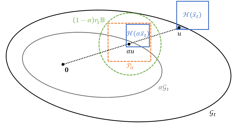
Figure 1: Graphical representation of the approach for lower bounding $\gamma_{t}$ (in ROFUL) for the setting with linked convex constraints.

In this section, we generalize the design and analysis of the algorithms ROFUL, Safe-PE and OPLB to a novel setting which we call linked convex constraints, where the output of the constraint function is multi-dimensional and must lie in an arbitrary convex set. The key challenge in this setting is characterizing how far a point in the optimistic action set is from the pessimistic action set. To address this, we leverage a theoretical tool from the zero-order optimization literature. We only provide a description of key contributions in this section and leave the details of the algorithms to Appendix E.

Problem description

The problem setting is specified as follows. At each round $t\in[T]$, the learner observes $z_{t}=Ax_{t}+\eta_{t}$, where $A\in\mathbb{R}^{n\times d}$ is the unknown constraint matrix and $\eta_{t}\in\mathbb{R}^{n}$ is a vector noise term. The learner must ensure that $Ax_{t}$ is in the known convex set $\mathcal{G}$ for all $t\in[T]$. The reward function and feedback mechanism are the same as the original setting described in Section 2. We assume that there exists $r>0$ such that $r\mathbb{B}\subseteq\mathcal{G}$. Lastly, we assume that each element of $\eta_{t}$ satisfies the assumptions on the noise used for ROFUL (Assumption 3) or Safe-PE (Assumption 8).

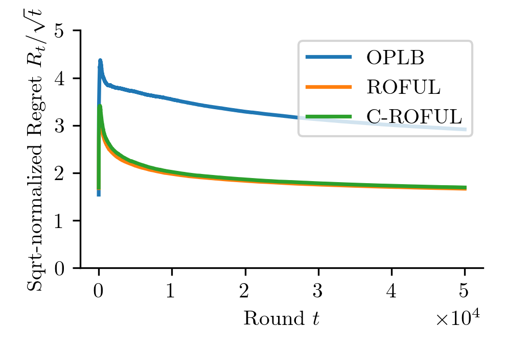
(a) Linear constraints.

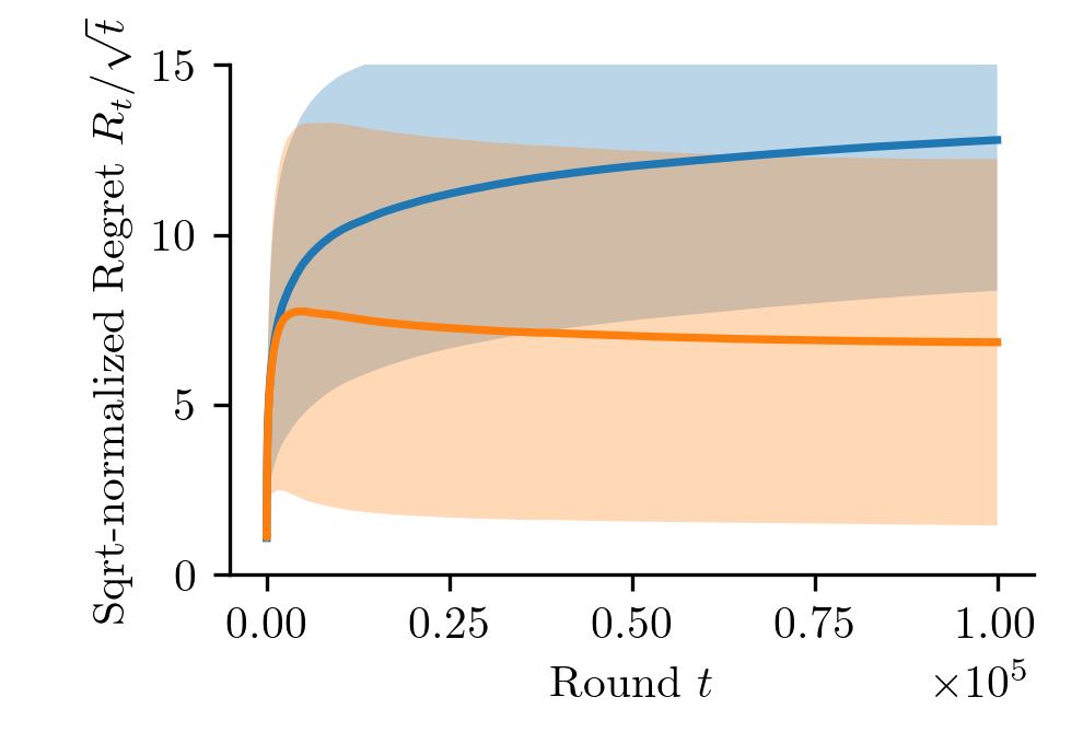
(b) Linked convex constraints.

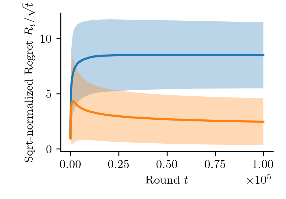
(c) Finite star-convex action set with linked convex constraints.

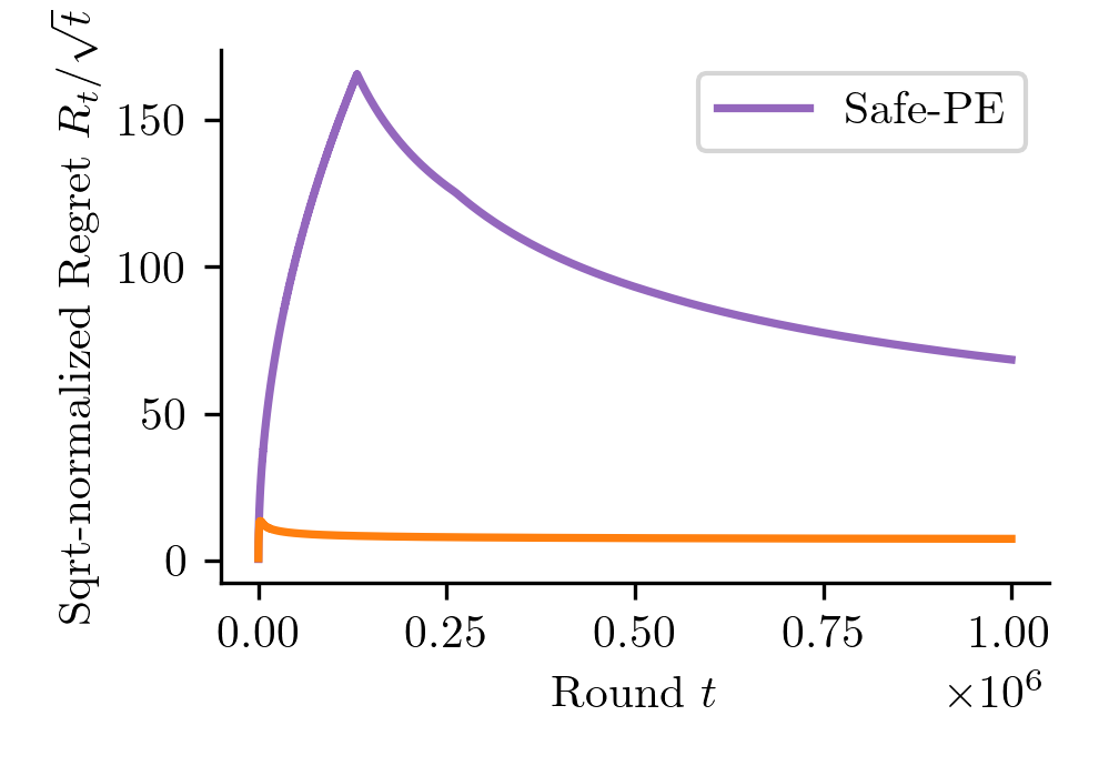
(d) Finite star-convex action set with linear constraints.

Figure 2: Simulation results of our proposed algorithms (ROFUL, C-ROFUL, Safe-PE) and OPLB Pacchiano et al. (2021).

Analysis techniques

Although the design of the algorithms trivially extends to this setting, the regret analysis is more challenging. In particular, it is difficult to characterize the distance from any point in the optimistic action set to the pessimistic action set. To address this, we use an analysis tool that is popular in the zero-order optimization literature (e.g. Flaxman et al. (2005)). This tool, given in Fact 1, allows us to consider a shrunk version of the constraint set in order to bound the scaling that is required to take any point in $\mathcal{Y}_{t}^{o}$ to $\mathcal{Y}_{t}^{p}$, i.e. $\gamma_{t}$ in ROFUL. We use a similar approach to bound the scaling required to take any point in $\mathcal{Y}$ to $\mathcal{Y}_{t}^{p}$ for OPLB and Safe-PE.

Fact 1.

Let $\mathcal{D}$ be a convex set such that $r\mathbb{B}\subseteq\mathcal{D}$ for some $r\geq 0$. Then, for any $\alpha\in[0,1]$ and $x\in\alpha\mathcal{D}$, it holds that $x+(1-\alpha)r\mathbb{B}\subseteq\mathcal{D}$.

With this in hand, we can then describe our approach for lower bounding $\gamma_{t}$, which is illustrated in Figure 1. Recall the definition of $\tilde{x}_{t}$ in ROFUL, where it is known that $\tilde{x}_{t}$ is in $\mathcal{Y}_{t}^{o}$. Then, the overall objective is to find some scaling $\alpha$ such that $\alpha\tilde{x}_{t}$ is in $\mathcal{Y}_{t}^{p}$ and then it follows that $\gamma_{t}\geq\alpha$. To do so, we define the uncertainty set for the constraint function at point $x$ as the box $\mathcal{H}(x):=\hat{a}_{t}^{\top}x+\beta_{t}\|x\|_{V_{t}^{-1}}\mathbb{B}_{\infty}$ and note that $\mathcal{Y}_{t}^{p}$ and $\mathcal{Y}_{t}^{o}$ are precisely the set of $x\in\mathcal{X}$ such that $\mathcal{H}(x)$ has nonempty intersection with $\mathcal{G}$ and the set of $x\in\mathcal{X}$ such that $\mathcal{H}(x)$ is contained in $\mathcal{G}$, respectively. First, we consider a point $u$ in the intersection of $\mathcal{G}$ and $\mathcal{H}(\tilde{x}_{t})$. Such a point exists given that $\tilde{x}_{t}$ is in $\mathcal{Y}_{t}^{o}$. Next, we scale $u$ by some non-negative scalar $\alpha$. Note that $\alpha u$ is in $\mathcal{H}(\alpha\tilde{x}_{t})$ given that $\mathcal{H}$ is positive homogeneous, i.e. $\alpha\mathcal{H}(x)=\mathcal{H}(\alpha x)$ for any $x$. In order to show that $\alpha\tilde{x}_{t}$ is in $\mathcal{Y}_{t}^{p}$, we need to show that $\mathcal{H}(\alpha\tilde{x}_{t})$ is contained in $\mathcal{G}$. To do so, we first consider a set $\mathcal{P}_{\alpha}$ that is centered at $\alpha u$ but has twice the radius of $\mathcal{H}(\alpha\tilde{x}_{t})$ and therefore contains $\mathcal{H}(\alpha\tilde{x}_{t})$ (this is illustrated in Figure 1). We then use Fact 1 to reason that, because $u$ is in $\mathcal{G}$, the ball $\alpha u+(1-\alpha)r_{1}\mathbb{B}$ is contained in $\mathcal{G}$. Therefore, we choose $\alpha$ such that $(1-\alpha)r_{1}\mathbb{B}=2\alpha\sqrt{n}\beta_{t}\|\tilde{x}_{t}\|_{V_{t}^{-1}}$, where the $\sqrt{n}$ is necessary to bound an infinity-norm ball with a 2-norm ball. Some simple algebra shows that $\gamma_{t}\geq 1-\frac{2\sqrt{n}}{r_{1}}\beta_{t}\|x_{t}\|_{V_{t}^{-1}}$.

6 Numerical experiments

In this section, we numerically validate the theoretical guarantees and assess the performance of the proposed algorithms. Note that we only give a high-level description of the simulations in this section. The details of the experimental settings are given in Appendix G.

Linear constraints

In this setting, we consider a problem with a box action set and a single linear constraint. We simulate ROFUL, C-ROFUL, Safe-LTS and OPLB for $30$ trials in this setting, where the reward vector, constraint vector, constraint limit and noise realizations were randomly sampled in each trial. The regret normalized by square root of $t$, and then averaged across all trials, is shown in Figure 2(a) for OPLB, ROFUL and C-ROFUL. Since the lines for all algorithms are trending below a constant, these results provide empirical evidence that all algorithms have regret bounded by a constant factor of $\sqrt{T}$, with ROFUL and C-ROFUL having lower average regret than OPLB for nearly the entire horizon. The results for Safe-LTS are deferred to Appendix G because its regret was significantly larger than either ROFUL or OPLB.

Linked convex constraints

We consider two different settings. In the first one, the action and constraint set are balls and in the second one, the action set is a finite star convex set and the constraint set is a ball. We simulated ROFUL and OPLB for $30$ trials in each setting, where the radius of the constraint set, the reward vector and the constraint vector were all randomly sampled. The average and standard deviation of the regret normalized by square root of $t$ is shown in Figure 2(b) and Figure 2(c) each setting. In both cases, ROFUL converges faster than OPLB to constant $\sqrt{t}$ regret

Finite star convex action set

In this setting, the action set consists only of the coordinate directions with scalings between $0$ and $1$, which can be viewed as a “star convex multi-armed bandit.” We also set the constraint and reward vectors to be $1$ at the first coordinate and $0$ elsewhere. We simulate both ROFUL and Safe-PE in this setting with $d=10$. The regret is shown in Figure 2(d). It is well known that UCB-based algorithms often empirically outperform elimination-based algorithms despite the orderwise tighter regret bound, as discussed by Valko et al. (2014) and Chu et al. (2011). Simulation results for PD-ROFUL are given in Appendix G.

7 Conclusion

In this work, we first introduce a novel algorithm, ROFUL, which has the advantage of being adaptive in comparison to existing algorithms. We then present two variants of this algorithm, PD-ROFUL, which enjoys nearly dimension-free regret, and C-ROFUL, which enjoys at least as good regret guarantees as existing algorithms while still being adaptive. When the action set is a finite-star convex set, we propose Safe-PE and show that it is possible to achieve improved regret guarantees. Lastly, we generalize all of these algorithms to the setting with linked convex constraints.

8 Acknowledgements

This work was supported by NSF grant #1847096.

Appendix A Proof of Theorem 1

First, we introduce some notation. Let the event that the confidence sets hold be defined as

$$\begin{split}\mathcal{E}_{\mathrm{conf}}:=\{&|x^{\top}(\hat{\theta}_{t}-\theta)|\leq\beta_{t}\|x\|_{V_{t}},\\ &|x^{\top}(\hat{a}_{t}-a)|\leq\beta_{t}\|x\|_{V_{t}},\forall x\in\mathcal{X},\forall t\geq 1\},\end{split}$$ (6)

and note that $\mathbb{P}(\mathcal{E}_{\mathrm{conf}})\geq 1-\delta$ by Lemma 1.

Then, we start by lower bounding $\gamma_{t}$.

Lemma 2.

If Assumption 1 and $\mathcal{E}_{\mathrm{conf}}$ holds, then

$$\gamma_{t}\geq\max\left(1-\frac{2}{b}\beta_{t}\|x_{t}\|_{V_{t}^{-1}},\nu\right)$$

for all $t\in[T]$.

Proof.

First we bound $\mu_{t}=\max\left\{\mu\in[0,1]:\mu\tilde{x}_{t}\in\mathcal{Y}_{t}^{p}\right\}$. In order to do so, we aim to find any $\alpha\in[0,1]$, such that $\alpha\tilde{x}_{t}\in\mathcal{Y}_{t}^{p}$. Firstly, the action set $\mathcal{X}$ is star-convex by Assumption 1, so we know that $\alpha\tilde{x}_{t}$ is in $\mathcal{X}$. Next, we need that $\alpha\hat{a}_{t}^{\top}\tilde{x}_{t}+\alpha\beta_{t}\|\tilde{x}_{t}\|_{V_{t}^{-1}}\leq b$. To show this, we choose $\alpha=\frac{b}{b+2\beta_{t}\|\tilde{x}_{t}\|_{V_{t}^{-1}}}$ such that $\alpha(b+\beta_{t}\|\tilde{x}_{t}\|_{V_{t}^{-1}})=b-\alpha\beta_{t}\|\tilde{x}_{t}\|_{V_{t}^{-1}}$ and use the fact that $\hat{a}_{t}^{\top}\tilde{x}_{t}-\beta_{t}\|\tilde{x}_{t}\|_{V_{t}^{-1}}\leq b$ to get that

$$\alpha\hat{a}_{t}^{\top}\tilde{x}_{t}\leq\alpha(\beta_{t}\|\tilde{x}_{t}\|_{V_{t}^{-1}}+b)=b-\alpha\beta_{t}\|\tilde{x}_{t}\|_{V_{t}^{-1}}.$$

Therefore, $\mu_{t}\geq\frac{b}{b+2\beta_{t}\|\tilde{x}_{t}\|_{V_{t}^{-1}}}$. Given that $\tilde{x}_{t}=x_{t}/\gamma_{t}$, this can be rearranged as

$$\gamma_{t} \geq\frac{1}{1+\frac{2}{b}\beta_{t}\|\tilde{x}_{t}\|_{V_{t}^{-1}}}=\frac{1}{1+\frac{2}{b\gamma_{t}}\beta_{t}\|x_{t}\|_{V_{t}^{-1}}}$$

$$\Longleftrightarrow\gamma_{t}\left(1+\frac{2}{b\gamma_{t}}\beta_{t}\|x_{t}\|_{V_{t}^{-1}}\right)\geq 1$$

$$\Longleftrightarrow\gamma_{t}\geq 1-\frac{2}{b}\beta_{t}\|x_{t}\|_{V_{t}^{-1}}.$$

Then, we can also use the fact that

$$\gamma_{t}\geq\tilde{b}_{t}=\min\left(\frac{\nu}{\|\tilde{x}_{t}\|},1\right)\geq\nu$$

to get that

$$\gamma_{t}\geq\max\left(1-\frac{2}{b}\beta_{t}\|x_{t}\|_{V_{t}^{-1}},\nu\right),$$

completing the proof. ∎

We will also need the so-called elliptic potential, which is standard in the stochastic linear bandit literature.

Lemma 3 (Lemma 11 in Abbasi-Yadkori et al. [2011]).

Consider a sequence $(w_{k})_{k\in\mathbb{N}}$ where $w_{k}\in\mathbb{R}^{d}$ and $\|w_{k}\|\leq 1$ for all $k\in\mathbb{N}$. Let $W_{k}=\lambda I+\sum_{s=1}^{k-1}w_{s}w_{s}^{\top}$ for some $\lambda\geq 1$. Then, it holds that

$$\sum_{k=1}^{K}\|w_{k}\|_{W_{k}^{-1}}^{2}\leq 2d\log\left(1+\frac{K}{\lambda d}\right).$$

We can then use the elliptic potential lemma and the lower bound on $\gamma_{t}$ to bound the instantaneous regret of the optimistic action.

Lemma 4.

Conditioned on $\mathcal{E}_{\mathrm{conf}}$, it holds that

$$\mathrm{Term\ I}=\theta^{\top}\left(x_{*}-\tilde{x}_{t}\right)\leq\frac{2}{\nu}\beta_{t}\|x_{t}\|_{V_{t}^{-1}}$$

Proof.

First note that, conditioned on $\mathcal{E}_{\mathrm{conf}}$, it holds for all $t\in[T]$ that

$$\theta^{\top}x_{*}\leq\max_{x\in\mathcal{Y}_{t}^{o}}\max_{\phi\in\mathcal{C}_{t}^{\theta}}\phi^{\top}x=\hat{\theta}_{t}^{\top}\tilde{x}_{t}+\beta_{t}\|\tilde{x}_{t}\|_{V_{t}^{-1}}.$$

Therefore, conditioning on $\mathcal{E}_{\mathrm{conf}}$ and using the fact that $\gamma_{t}\geq\nu$ by Lemma 2, we have for all $t\in[T]$ that

$$\theta^{\top}x_{*}-\theta^{\top}\tilde{x}_{t} \leq\hat{\theta}_{t}^{\top}\tilde{x}_{t}+\beta_{t}\|\tilde{x}_{t}\|_{V_{t}^{-1}}-\theta^{\top}\tilde{x}_{t}$$

$$\leq 2\beta_{t}\|\tilde{x}_{t}\|_{V_{t}^{-1}}$$

$$=\frac{2\beta_{t}}{\gamma_{t}}\|x_{t}\|_{V_{t}^{-1}}$$

$$\leq\frac{2}{\nu}\beta_{t}\|x_{t}\|_{V_{t}^{-1}},$$

which completes the proof. ∎

Then, we bound the reward difference between the optimistic action and the played action.

Lemma 5.

Let Assumption 1 hold. Then, conditioned on $\mathcal{E}_{\mathrm{conf}}$, it holds that

$$\mathrm{Term\ II}=\theta^{\top}(\tilde{x}_{t}-x_{t})\leq S_{\theta}\frac{2\beta_{t}}{b}\|x_{t}\|_{V_{t}^{-1}}$$

for all $t\in[T]$.

Proof.

Since $\gamma_{t}\leq 1$ by definition and $\|\theta\|\leq S$ by Assumption 2, we have that

$$\theta^{\top}(\tilde{x}_{t}-x_{t}) =\theta^{\top}(\tilde{x}_{t}-\gamma_{t}\tilde{x}_{t})$$

$$=(1-\gamma_{t})\theta^{\top}\tilde{x}_{t}$$

$$\leq(1-\gamma_{t})\|\theta\|\|\tilde{x}_{t}\|$$

$$\leq(1-\gamma_{t})S_{\theta}$$

$$\leq S_{\theta}\frac{2\beta_{t}}{b}\|x_{t}\|_{V_{t}^{-1}},$$

where the last inequality follows from Lemma 2. ∎

Lastly, we can put everything together to get the complete regret bound, which is a restatement of Theorem 1.

Theorem 4 (Duplicate of Theorem 1).

Let Assumptions 1, 3 and 2 hold. Then, the regret of ROFUL (Algorithm 1) satisfies

$$R_{T}\leq\left(\frac{S_{\theta}}{b}+\frac{1}{\nu}\right)\beta_{T}\sqrt{8dT\log\left(1+\frac{T}{\lambda d}\right)}$$

with probability at least $1-\delta$.

Proof.

Conditioning on $\mathcal{E}_{\mathrm{conf}}$ and using Lemmas 5 and 4, it holds that

$$r_{t} :=\theta^{\top}\left(x_{*}-x_{t}\right)$$

$$=\theta^{\top}\left(x_{*}-\tilde{x}_{t}\right)+\theta^{\top}\left(\tilde{x}_{t}-x_{t}\right)$$

$$\leq\left(\frac{S_{\theta}}{b}+\frac{1}{\nu}\right)2\beta_{t}\|x_{t}\|_{V_{t}^{-1}}$$

We can use Lemma 3 to get that

$$\sum_{t=1}^{T}r_{t}^{2} \leq\sum_{t=1}^{T}\left(\frac{S_{\theta}}{b}+\frac{1}{\nu}\right)^{2}4\beta_{t}\|x_{t}\|_{V_{t}^{-1}}^{2}$$

$$\leq\left(\frac{S_{\theta}}{b}+\frac{1}{\nu}\right)^{2}8d\beta_{T}^{2}\log\left(1+\frac{T}{\lambda d}\right)$$

The proof is completed by applying Cauchy-Schwarz. ∎

Appendix B Proof of Theorem 2

First we prove Theorem 2 and then will turn our attention to Corollary 1.

Theorem 5 (Duplicate of Theorem 2).

Let Assumptions 1, 3 and 2 hold. If $\Delta>0$, then the number of wrong directions chosen by RO-SLB (Algorithm 1) satisfies

$$B_{T}\leq\frac{32d\beta_{T}^{2}}{\nu^{2}\Delta^{2}}\log\left(1+\frac{T}{\lambda d}\right)$$

with probability at least $1-\delta$.

Proof.

We condition on $\mathcal{E}_{\mathrm{conf}}$ (in (6)) throughout. Let $v_{t}:=\alpha_{t}x_{t}$, where $\alpha_{t}:=\max\{\alpha:\alpha x_{t}\in\mathcal{Y}\}$.

First, we argue that $\|v_{t}\|\in[\|x_{t}\|,\|\tilde{x}_{t}\|]$. Note that by Assumption 1, it holds that $\hat{\theta}_{t}^{\top}\tilde{x}_{t}+\beta_{t}\|\tilde{x}_{t}\|_{V_{t}^{-1}}\geq\theta^{\top}x_{*}>0$. It follows that $\tilde{x}_{t}$ cannot be scaled up anymore while still being in $\mathcal{Y}_{t}^{o}$, i.e. $\tilde{x}_{t}=\tilde{\alpha}_{t}v_{t}$ where $\tilde{\alpha}_{t}=\max\{\alpha:\alpha v_{t}\in\mathcal{Y}_{t}^{o}\}$. Since $\mathcal{Y}_{t}^{o}$ is a superset of $\mathcal{Y}$, it holds that $\|v_{t}\|\leq\|\tilde{x}_{t}\|$. Also, since $x_{t}\in\mathcal{Y}$, it follows that $\|x_{t}\|\leq\|v_{t}\|$, by definition. Therefore, we have that

$$\theta^{\top}(\tilde{x}_{t}-v_{t})\leq S\|\tilde{x}_{t}-x_{t}\|\leq S(1-\gamma_{t})\leq\frac{2S}{b}\beta_{t}\|x_{t}\|_{V_{t}^{-1}}.$$

In order to bound the number of times that the wrong action is chosen, we study the regret due to the wrong choice of direction,

$$\tilde{R}_{T}:=\sum_{t=1}^{T}\theta^{\top}(x_{*}-v_{t}).$$

We will denote the instaneous regret due to the wrong choice of direction as $\tilde{r}_{t}=\theta^{\top}(x_{*}-v_{t})$. Note that either $\tilde{r}_{t}=0$ if the correct direction is chosen or $\tilde{r}_{t}\geq\Delta$ if the wrong direction is chosen. Therefore,

$$\tilde{R}_{T}:=\sum_{t=1}^{T}\tilde{r}_{t} =\sum_{t=1}^{T}\tilde{r}_{t}\mathds{1}\{\nexists\ \alpha>0:x_{t}=\alpha x_{*}\}$$

$$\geq\Delta\sum_{t=1}^{T}\mathds{1}\{\nexists\ \alpha>0:x_{t}=\alpha x_{*}\}$$

$$=\Delta B_{T}$$

Since $\tilde{R}_{T}\geq\Delta B_{T}$, an upper bound on $\tilde{R}_{T}$ implies an upper bound on $B_{T}$.

Then, we bound $\tilde{r}_{t}$ in the following,

$$\tilde{r}_{t} =\theta^{\top}x_{*}-\theta^{\top}v_{t}$$

$$\leq\hat{\theta}_{t}^{\top}\tilde{x}_{t}+\beta_{t}\|\tilde{x}_{t}\|_{V_{t}^{-1}}-\theta^{\top}v_{t}$$

$$=\theta^{\top}\tilde{x}_{t}+(\theta-\hat{\theta}_{t})^{\top}\tilde{x}_{t}+\beta_{t}\|\tilde{x}_{t}\|_{V_{t}^{-1}}-\theta^{\top}v_{t}$$

$$\leq\theta^{\top}\tilde{x}_{t}+2\beta_{t}\|\tilde{x}_{t}\|_{V_{t}^{-1}}-\theta^{\top}v_{t}$$

$$=\theta^{\top}(\tilde{x}_{t}-v_{t})+2\beta_{t}\|\tilde{x}_{t}\|_{V_{t}^{-1}}$$

$$\leq\frac{2S}{b}\beta_{t}\|x_{t}\|_{V_{t}^{-1}}+\frac{2}{\nu}\beta_{t}\|x_{t}\|_{V_{t}^{-1}}$$

Also, note that $\tilde{r}_{t}\leq(\tilde{r}_{t})^{2}/\Delta$. Then, using Lemma 3, we have that

$$\tilde{R}_{T} \leq\sum_{t=1}^{T}\frac{(\tilde{r}_{t})^{2}}{\Delta}$$

$$\leq\frac{16S^{2}\beta_{T}^{2}}{b^{2}\Delta}\sum_{t=1}^{T}\|\tilde{x}_{t}\|_{V_{t}^{-1}}^{2}$$

$$\leq\frac{32S^{2}\beta_{T}^{2}d}{b^{2}\Delta}\log\left(1+\frac{T}{\lambda d}\right)$$

and therefore,

$$B_{T}\leq\frac{\tilde{R}_{T}}{\Delta}\leq\frac{32S^{2}\beta_{T}^{2}d}{b^{2}\Delta^{2}}\log\left(1+\frac{T}{\lambda d}\right).$$

∎

Now, we turn out attention to Corollary 1. To do so, we state PD-ROFUL more formally in Algorithm 2. Note that the second phase of the algorithm utilizes a one-dimensional least-squares estimator and confidence set. This is done by playing $\xi_{t}u_{*}$ where $u_{*}$ is the optimal direction, as identified in the first phase of the algorithm, and $\xi_{t}$ is the chosen scalar at round $t$. Therefore, the feedback is $z_{t}=\xi_{t}a^{\top}u_{*}+\eta_{t}$ and it becomes an estimation task for the scalar $\phi:=a^{\top}u_{*}$. As such, the algorithm uses the least-squares estimator and the confidence sets for $\phi$.

1 Set $\mathcal{A}=()$, $N=0$ and $t=1$.

2 while $N\leq\bar{B}=\frac{32S^{2}d}{b^{2}\Delta^{2}}\beta_{T}^{2}\log\left(1+\frac{T}{\lambda d}\right)$ do

3       ROFUL plays $x_{t}$ and observes $y_{t},z_{t}$.

4       Update $\mathcal{A}=\left(\mathcal{A},\frac{x_{t}}{\|x_{t}\|}\right)$.

5       Set $N=\max_{A\in\mathcal{A}}\sum_{D\in\mathcal{A}}\mathds{1}\{A=D\}$.

6       Set $t=t+1$.

7      

8 end while

9Set $u_{*}=\operatorname*{arg\,max}_{A\in\mathcal{A}}\sum_{D\in\mathcal{A}}\mathds{1}\{A=D\}$ and $\tau=t$.

10 Let $\Xi=\{\xi:\xi u_{*}\in\mathcal{X}\}$ and $\tilde{\beta}_{t}:=\rho\sqrt{\log\left(\frac{1+(t-\tau)/\lambda}{\delta/2}\right)}+\sqrt{\lambda}S$.

11 for $t=\tau+1$ to $T$ do

12       Calculate $\hat{\phi}_{t}=\frac{1}{V_{t}}\sum_{s=\tau+1}^{t-1}\xi_{s}z_{s}$ where $V_{t}=\lambda+\sum_{s=\tau+1}^{t-1}\xi_{s}^{2}$.

13       Set $\Xi_{t}^{p}=\{\xi\in\Xi:\hat{\phi}_{t}\xi+\tilde{\beta}_{t}\frac{|\xi|}{\sqrt{V_{t}}}\leq b\}$.

14       Find $\xi_{t}=\max\Xi_{t}^{p}$.

15       Play $x_{t}=\xi_{t}u_{*}$ and observe $z_{t}$.

16      

17 end for

Algorithm 2 Problem-Dependent ROFUL (PD-ROFUL)

Corollary 3 (Duplicate of Corollary 1).

Let Assumptions 1, 3 and 2 hold. With $\Delta>0$, the regret of PD-ROFUL (Algorithm 2) satisfies

$$R_{T} \leq\frac{8S}{b}\beta_{2\bar{B}}\sqrt{d\bar{B}\log\left(1+\frac{2\bar{B}}{\lambda d}\right)}$$

$$+\frac{2S}{b}\tilde{\beta}_{T}\sqrt{8T\log\left(1+\frac{T}{\lambda d}\right)}$$

with probability at least $1-2\delta$, where $\tilde{\beta}_{T}$ is $\beta_{T}$ with $d=1$.

Proof.

We condition on the confidence sets holding jointly for both the first and second phases, which occurs with probability at least $1-2\delta$. We use the regret decomposition

$$R_{T}=\underbrace{\sum_{t=1}^{\tau-1}r_{t}}_{R_{T}^{I}}+\underbrace{\sum_{t=\tau}^{T}r_{t}}_{R_{T}^{II}}$$

From Theorem 2, we know that ROFUL ensures that $B_{T}\leq\bar{B}$. Therefore if a single action is played more than $\bar{B}$ times, it must be the optimal action. It follows that the algorithm correctly identifies $u_{*}$ as the optimal direction. Since wrong directions are played less than $\bar{B}$ times, it follows that the first phase of the algorithm is no longer than $2\bar{B}$ and therefore $\tau-1\leq 2\bar{B}$. Therefore, we know that

$$R_{T}^{I}=\sum_{t=1}^{\tau-1}r_{t} \leq\frac{2S}{b}\beta_{\tau-1}\sqrt{8d(\tau-1)\log\left(1+\frac{\tau-1}{\lambda d}\right)}$$

$$\leq\frac{2S}{b}\beta_{2\bar{B}}\sqrt{8d(2\bar{B})\log\left(1+\frac{2\bar{B}}{\lambda d}\right)},$$

where the second inequality holds because the first line is increasing with $\tau-1$ and $\tau-1\leq 2\bar{B}$.

For the remainder of the rounds, play of the algorithm is equivalent to ROFUL with $d=1$ because there is no direction to choose so the action will always be the maximum of $\Xi$. Therefore, the regret during this period is less than that given in Theorem 1 with $d=1$. ∎

Appendix C Proof of Proposition 1

In this section, we show that ROFUL can be stated in a way that allows direct comparison to OPLB and then design an algorithm that chooses the better update of the two algorithms at each time step.

Before getting to it, we prove a lemma which we will use to show that the maximizer of an upper confidence bound over a compact set is within the maximally scaled part of the set.

Lemma 6.

Let $f:\mathbb{R}^{d}\rightarrow\mathbb{R}$ be a function satisfying $f(\alpha x)=\alpha f(x)$ for all $\alpha\geq 0$ and $\mathcal{D}$ be a compact set. Also, define $\bar{\mathcal{D}}=\{x\in\mathcal{D}:\zeta x\not\in\mathcal{D}\ \forall\zeta>1\}$. If there exists a $w\in\mathcal{D}$ such that $f(w)>0$, then it holds that $\operatorname*{arg\,max}_{x\in\mathcal{D}}f(x)=\bar{\mathcal{D}}$.

Proof.

Let $\mathcal{D}_{*}=\operatorname*{arg\,max}_{x\in\mathcal{D}}f(x)$. Since there exists a $w\in\mathcal{D}$ such that $f(w)>0$, the maximum must be at least this large so every $y\in\mathcal{D}_{*}$ must satisfy $f(y)>0$.

We then prove the statement of the lemma. Suppose that there exists a $v\in\mathcal{D}_{*}$ such that $v$ is not in $\bar{\mathcal{D}}$. It follows that there exists a $\zeta>1$ such that $\zeta v\in\mathcal{D}$. However, $f(\zeta v)=\zeta f(v)>f(v)$ so $v$ cannot be in $\mathcal{D}_{*}$. The statement of the lemma follows. ∎

Using this, we then show that the actions chosen by ROFUL are equivalent to a upper confidence bound-type selection rule where the scaling of the upper-confidence bound is chosen according to the specific point in the pessimistic set.

Proposition 2 (Duplicate of Proposition 1).

Let Assumption 1 hold, and define $\hat{\mathcal{Y}}_{t}^{p}:=\mathcal{Y}_{t}^{p}\cup(\nu\mathbb{B}\cap\mathcal{Y}_{t}^{o})$ and $\bar{\mathcal{Y}}_{t}^{p}:=\{x\in\hat{\mathcal{Y}}_{t}^{p}:\zeta x\not\in\hat{\mathcal{Y}}_{t}^{p}\ \forall\zeta>1\}$. Then, conditioned on the confidence sets in Lemma 1 holding for all rounds, ROFUL (Algorithm 1) is equivalent to an algorithm that, for all $t\in[T]$, chooses

$$x_{t}\in\operatorname*{arg\,max}_{x\in\bar{\mathcal{Y}}_{t}^{p}}\left(\hat{\theta}_{t}^{\top}x+\kappa_{t}(x)\beta_{t}\|x\|_{V_{t}^{-1}}\right),$$ (7)

where,

$$\kappa_{t}(x):=(\alpha_{t}(x)-1)\frac{\hat{\theta}_{t}^{\top}x}{\beta_{t}\|x\|_{V_{t}^{-1}}}+\alpha_{t}(x),$$

and $\alpha_{t}(x):=\max\{\mu\geq 0:\mu x\in\mathcal{Y}_{t}^{o}\}$.

Proof.

We condition on $\mathcal{E}_{\mathrm{conf}}$ in (6) throughout. Let $\bar{\mathcal{Y}}_{t}^{o}:=\{x\in\mathcal{Y}_{t}^{o}:\zeta x\not\in\mathcal{Y}_{t}^{o}\ \forall\zeta>1\}$ which is the set of points in $\mathcal{Y}_{t}^{o}$ that cannot be scaled up further while still being in $\mathcal{Y}_{t}^{o}$. Since $\hat{\theta}_{t}^{\top}x+\beta_{t}\|x\|_{V_{t}^{-1}}\geq\theta^{\top}x_{*}>0$ conditioned on $\mathcal{E}_{\mathrm{conf}}$ in (6), we know by Lemma 6 that any maximizer of $\hat{\theta}_{t}^{\top}x+\beta_{t}\|x\|_{V_{t}^{-1}}$ over $\mathcal{Y}_{t}^{o}$ belongs to $\bar{\mathcal{Y}}_{t}^{o}$.

Let $\Gamma_{t}(x):=x(\max\{\mu\in[0,1]:\mu x\in\nu\mathbb{B}\cup\mathcal{Y}_{t}^{p}\})$ be a function that scales an action in to the union of the pessimistic set and a ball of radius $\nu$. Note that the algorithm chooses actions as $x_{t}=\Gamma_{t}(\tilde{x}_{t})$. With some abuse of notation, we will use $\Gamma_{t}(\bar{\mathcal{Y}}_{t}^{o})$ to mean the set of points formed by applying $\Gamma_{t}$ to each point in $\bar{\mathcal{Y}_{t}^{o}}$.

We now argue that $\Gamma_{t}(\bar{\mathcal{Y}}_{t}^{o})$ is equal to $\bar{\mathcal{Y}}_{t}^{p}$ and that $\alpha_{t}(\bar{\mathcal{Y}}_{t}^{p})$ is equal to $\bar{\mathcal{Y}}_{t}^{o}$. Note that there always exists an $\epsilon>0$, such that $\epsilon\mathbb{B}\cap\mathcal{X}\subseteq\mathcal{Y}_{t}^{p}\subseteq\hat{\mathcal{Y}}_{t}^{p}$. To see this, note that, since $b>0$, there exists an $\epsilon>0$ such that, for and all $u\in\mathbb{B}$, it holds that $\epsilon(\hat{a}_{t}^{\top}u+\beta_{t}\|u\|_{V_{t}^{-1}})\leq b$. Therefore, for every point in $\mathcal{X}$, there exists an $x$ in $\hat{\mathcal{Y}}_{t}^{p}$ that can be scaled to reach that point and vice versa (since $\mathcal{X}$ is star convex). Since $\bar{\mathcal{Y}}_{t}^{p}$ is simply the maximum scaling of each point in $\hat{\mathcal{Y}}_{t}^{p}$, the same holds for $\bar{\mathcal{Y}}_{t}^{p}$. It follows that $\alpha_{t}(\bar{\mathcal{Y}}_{t}^{p})=\bar{\mathcal{Y}}_{t}^{o}$ and $\Gamma_{t}(\bar{\mathcal{Y}}_{t}^{o})=\bar{\mathcal{Y}}_{t}^{p}$.

Therefore, we know that the actions played by the algorithm are in the set

$$\Gamma_{t}\left(\operatorname*{arg\,max}_{x\in\mathcal{Y}_{t}^{o}}\left(\hat{\theta}_{t}^{\top}x+\beta_{t}\|x\|_{V_{t}^{-1}}\right)\right)$$

$$=\Gamma_{t}\left(\operatorname*{arg\,max}_{x\in\bar{\mathcal{Y}}_{t}^{o}}\left(\hat{\theta}_{t}^{\top}x+\beta_{t}\|x\|_{V_{t}^{-1}}\right)\right)$$

$$=\operatorname*{arg\,max}_{y\in\Gamma_{t}(\bar{\mathcal{Y}}_{t}^{o})}\alpha_{t}(y)\left(\hat{\theta}_{t}^{\top}y+\beta_{t}\|y\|_{V_{t}^{-1}}\right)$$

$$=\operatorname*{arg\,max}_{y\in\bar{\mathcal{Y}}_{t}^{p}}\alpha_{t}(y)\left(\hat{\theta}_{t}^{\top}y+\beta_{t}\|y\|_{V_{t}^{-1}}\right)$$

$$=\operatorname*{arg\,max}_{y\in\bar{\mathcal{Y}}_{t}^{p}}\left(\hat{\theta}_{t}^{\top}y+\kappa_{t}(y)\beta_{t}\|y\|_{V_{t}^{-1}}\right).$$

∎

Now, we prove Corollary 2, which shows that we can choose the smaller of the two $\kappa$ values.

Corollary 4 (Duplicate of Corollary 2).

Let Assumptions 1, 2 and 3 hold. Consider the algorithm C-ROFUL, which chooses actions for all $t\in[T]$ as

$$x_{t}\in\operatorname*{arg\,max}_{x\in\bar{\mathcal{Y}}_{t}^{p}}\left(\hat{\theta}_{t}^{\top}x+\tilde{\kappa}_{t}(x)\beta_{t}\|x\|_{V_{t}^{-1}}\right),$$ (8)

where $\tilde{\kappa}_{t}(x)=\min(\kappa_{t}(x),1+\frac{2S_{\theta}}{b})$. Then, the regret of C-ROFUL satisfies

$$R_{T}\leq 2\left(1+\frac{S_{\theta}}{b}\right)\beta_{T}\sqrt{2dT\log\left(1+\frac{T}{\lambda d}\right)},$$

with probability at least $1-\delta$.

Proof.

First, consider the case where the $\tilde{\kappa}_{t}(x_{t})=\bar{\kappa}:=1+\frac{S_{\theta}}{b}$. Then, note that

$$\max_{x\in\bar{\mathcal{Y}}_{t}^{p}}\left(\hat{\theta}_{t}^{\top}x+\bar{\kappa}\beta_{t}\|x\|_{V_{t}^{-1}}\right)$$

$$=\max_{x\in\hat{\mathcal{Y}}_{t}^{p}}\left(\hat{\theta}_{t}^{\top}x+\bar{\kappa}\beta_{t}\|x\|_{V_{t}^{-1}}\right)$$

$$\geq\max_{x\in\mathcal{Y}_{t}^{p}}\left(\hat{\theta}_{t}^{\top}x+\bar{\kappa}\beta_{t}\|x\|_{V_{t}^{-1}}\right)\geq\theta^{\top}x_{*}$$

from the analysis of the OPLB algorithm in Appendix E. Then, note that optimism also holds if $\tilde{\kappa}_{t}(x_{t})=\kappa_{t}(x)$ as

$$\max_{x\in\bar{\mathcal{Y}}_{t}^{p}}\left(\hat{\theta}_{t}^{\top}x+\kappa_{t}(x)\beta_{t}\|x\|_{V_{t}^{-1}}\right)$$

$$=\max_{x\in\bar{\mathcal{Y}}_{t}^{p}}\alpha_{t}(x)\left(\hat{\theta}_{t}^{\top}x+\beta_{t}\|x\|_{V_{t}^{-1}}\right)$$

$$=\max_{x\in\mathcal{Y}_{t}^{o}}\left(\hat{\theta}_{t}^{\top}x+\beta_{t}\|x\|_{V_{t}^{-1}}\right)\geq\theta^{\top}x_{*},$$

from the analysis of ROFUL. Therefore, we have that

$$r_{t} =\theta^{\top}x_{*}-\theta^{\top}x_{t}$$

$$\leq\hat{\theta}_{t}^{\top}x_{t}+\tilde{\kappa}_{t}(x_{t})\beta_{t}\|x_{t}\|_{V_{t}^{-1}}-\theta^{\top}x_{t}$$

$$\leq(1+\tilde{\kappa}_{t}(x_{t}))\beta_{t}\|x_{t}\|_{V_{t}^{-1}}$$

$$\leq(2+\frac{2S_{\theta}}{b})\beta_{t}\|x_{t}\|_{V_{t}^{-1}}.$$

The rest of the proof follows from typical methods. ∎

Appendix D Details of Safe-PE Algorithm

Input: $\mathcal{X},S,b,d,\rho,\delta\in(0,1),\lambda\geq 1$

1 Set $\mathcal{A}_{1}=[k]$, $\zeta_{i,0}=\min(b/S,\alpha_{i})\ \forall i\in[k]$, $\mathcal{Y}_{0}^{p}=\{\zeta_{i,0}u_{i}\}_{i\in[k]}$, $J=\lceil\log_{2}(T)\rceil$, $t_{j}=2^{j-1}$, $\bar{V}_{0}=\lambda I$.

2 for $j=1$ to $J$ do

3       $V_{t_{j}}=\lambda I$.

4       for $t=t_{j}$ to $\min(t_{j+1}-1,T)$ do

5             Play $x_{t}\in\operatorname*{arg\,max}_{x\in\mathcal{Y}_{j}^{p}}\|x\|_{V_{t}^{-1}}$.

6             $V_{t+1}=V_{t}+x_{t}x_{t}^{\top}$.

7            

8       end for

9      Set $\hat{\theta}_{j}=\bar{V}_{j}^{-1}\sum_{s=t_{j}}^{t_{j+1}}x_{s}y_{s}$ and $\hat{a}_{j}=\bar{V}_{j}^{-1}\sum_{s=t_{j}}^{t_{j+1}}x_{s}z_{s}$, where $\bar{V}_{j}=V_{t_{j+1}}$.

10       Find $\hat{x}_{j}\in\operatorname*{arg\,max}_{x\in\mathcal{Y}_{j}^{p}}\left(\hat{\theta}_{j}^{\top}x-\beta\|x\|_{\bar{V}_{j}^{-1}}\right)$.

11       Update $\mathcal{A}_{j+1}=\left\{i\in\mathcal{A}_{j}:\hat{\theta}_{j}^{\top}(\hat{x}_{j}-\zeta_{i,j}u_{i})\leq\beta\|\hat{x}_{j}\|_{\bar{V}_{j}^{-1}}+\beta\zeta_{i,j}\|u_{i}\|_{\bar{V}_{j}^{-1}}+\frac{2S\beta\zeta_{i,j}\|u_{i}\|_{\bar{V}_{j-1}^{-1}}}{b}\right\}$.

12       Update $\mu_{i,j+1}:=\max\left\{\alpha\in[0,\alpha_{i}]:\alpha\left(u_{i}^{\top}\hat{a}_{j}+\|u_{i}\|_{\bar{V}_{j}^{-1}}\beta\right)\leq b\right\}$ and $\zeta_{i,j+1}=\max\left(\zeta_{i,j},\mu_{i,j+1}\right)$ for all $i\in\mathcal{A}_{j+1}$.

13       Update $\mathcal{Y}_{j+1}^{p}=\{\zeta_{i,j+1}u_{i}\}_{i\in\mathcal{A}_{j+1}}$.

14      

15 end for

Algorithm 3 Safe Phased Elimination (Safe-PE)

In this section, we give the details of the Safe-PE algorithm (Algorithm 3) discussed in Section 4. This algorithm relies on the action set being a finite star convex set, which we formally assume in the following.

Assumption 5.

The action set satisfies

$$\mathcal{X}:=\bigcup_{i\in[k]}\{\alpha u_{i}:\alpha\in[0,\alpha_{i}]\},$$

where $u_{1},...,u_{k}\in\mathbb{S}$ are unit vectors and $\alpha_{1},...,\alpha_{k}\in\mathbb{R}_{+}$ are the maximum scalings for each unit vectors.

The Safe-PE algorithm builds on SpectralEliminator from Valko et al. [2014] and Kocák et al. [2020]. It differs in that it eliminates directions in each phase rather than distinct actions and only plays actions from a verifiably safe set.

D.1 Operation of algorithm

The Safe-PE algorithm consists of phases $j=1,2,...$, which are each of duration $2^{j}$. Throughout its operation, the algorithm maintains a set of direction indexes $\mathcal{A}_{j}$ and safe actions $\mathcal{Y}_{j}^{p}$. The key parts of each phase are:

1. For $2^{j}$ rounds, chooses the action in $\mathcal{Y}_{j}^{p}$ with the largest confidence set width $\|\cdot\|_{V_{t}^{-1}}$ (line 3).

2. Eliminates directions from $\mathcal{A}_{j}$ with too low of estimated reward (line 3).

3. Updates $\mathcal{Y}_{j}^{p}$ with the maximum scaling of each direction that is verifiably safe (lines 3 and 3).

The algorithm relies on a confidence set to determine which directions should be eliminated and to ensure that the constraints are not violated. Different from the confidence set in Lemma 1, the radius of the following confidence set does not grow with $d$. We prove such a confidence set in the following lemma.

Lemma 7.

Let Assumptions 4 and 5 hold and fix some $\delta\in(0,1)$. Then, for all $x\in\mathcal{X}$ and all $j\in[J]$ it holds that $|x^{\top}(\hat{\theta}_{j}-\theta)|\leq\|x\|_{V_{j}^{-1}}\beta$ and $|x^{\top}(\hat{a}_{j}-a)|\leq\|x\|_{V_{j}^{-1}}\beta$ where $\beta=\rho\sqrt{2\log\left(\frac{4kJ}{\delta}\right)}+\sqrt{\lambda}S$ with probability at least $1-\delta$.

Proof.

First, we find a confidence set that applies for a single $u\in\{u_{1},...,u_{k}\}$. To do so, we start as

$$u^{\top}(\hat{\theta}_{j}-\theta) =u^{\top}\left(\bar{V}_{j}^{-1}\sum_{t=t_{j}}^{t_{j+1}-1}x_{t}y_{t}-\theta\right)$$

$$=u^{\top}\left(\bar{V}_{j}^{-1}\sum_{t=t_{j}}^{t_{j+1}-1}x_{t}(x_{t}^{\top}\theta+\epsilon_{t})-\theta\right)$$

$$=\underbrace{u^{\top}\left(\bar{V}_{j}^{-1}\sum_{t=t_{j}}^{t_{j+1}-1}x_{t}x_{t}^{\top}-I\right)\theta}_{\mathrm{Term\ I}}+\underbrace{u^{\top}\bar{V}_{j}^{-1}\sum_{t=t_{j}}^{t_{j+1}-1}x_{t}\epsilon_{t}}_{\mathrm{Term\ II}}$$

Using the notation $\tilde{V}=\sum_{t=t_{j}}^{t_{j+1}-1}x_{s}x_{s}^{\top}$, we study the first term,

$$|\mathrm{Term\ I}| =\left|u^{\top}\left(\bar{V}_{j}^{-1}\tilde{V}-I\right)\theta\right|$$

$$=\left|u^{\top}\bar{V}_{j}^{-1}\left(\tilde{V}-\bar{V}_{j}\right)\theta\right|$$

$$=\lambda\left|u^{\top}\bar{V}_{j}^{-1}\theta\right|$$

$$\leq\sqrt{\lambda}\|\theta\|\|u^{\top}\bar{V}_{j}^{-1}\sqrt{\lambda}I\|$$

$$=\sqrt{\lambda}\|\theta\|\sqrt{u^{\top}\bar{V}_{j}^{-1}\lambda I\bar{V}_{j}^{-1}u}$$

$$\leq\sqrt{\lambda}S\|u\|_{\bar{V}_{j}^{-1}},$$

where we use the fact that $\bar{V}_{j}\succeq\lambda I$. Now, we look at the second term. Because $\epsilon_{t}$ are subgaussian and independent from eachother and all $x_{t}$ for $t\in[t_{j},t_{j+1}-1]$, we know that

$$\mathbb{P}\left(|\mathrm{Term\ II}|>\rho\sqrt{2\log\left(\frac{2}{\delta^{\prime}}\right)\sum_{t=t_{j}}^{t_{j+1}-1}(u^{\top}\bar{V}_{j}^{-1}x_{s})^{2}}\right)\leq\delta^{\prime}.$$

Since $\tilde{V}\preceq\bar{V}_{j}$,

$$\sum_{t=t_{j}}^{t_{j+1}-1}(u^{\top}\bar{V}_{j}^{-1}x_{s})^{2}=u^{\top}\bar{V}_{j}^{-1}\tilde{V}\bar{V}_{j}^{-1}u\leq u^{\top}\bar{V}_{j}^{-1}\bar{V}_{j}\bar{V}_{j}^{-1}u=\|u\|_{\bar{V}_{j}^{-1}}^{2}.$$

Therefore, with probability at least $1-\delta^{\prime}$, it holds that

$$|u^{\top}(\hat{\theta}_{j}-\theta)|\leq|\mathrm{Term\ I}|+|\mathrm{Term\ II}|\leq\left(\rho\sqrt{2\log\left(\frac{2}{\delta^{\prime}}\right)}+\sqrt{\lambda}S\right)\|u\|_{\bar{V}_{j}^{-1}}.$$

Note that the same applies replacing $\theta$ with $a$. Then, by taking $\delta^{\prime}=(2Jk)/\delta$, it holds that $|u^{\top}(\hat{\theta}_{j}-\theta)|\leq\beta\|u\|_{\bar{V}_{j}^{-1}}$ and $|u^{\top}(\hat{a}_{j}-a)|\leq\beta\|u\|_{\bar{V}_{j}^{-1}}$ for all $u\in\{u_{1},...,u_{k}\}$ and all $j\in[J]$ with probability at least $1-\delta$. Since all $x\in\mathcal{X}$ can be written as $\alpha u$ for some $\alpha\geq 0$ and $u\in\{u_{1},...,u_{k}\}$, it holds under the same conditions that

$$|x^{\top}(\hat{\theta}_{j}-\theta)|=\alpha|u^{\top}(\hat{\theta}_{j}-\theta)|\leq\alpha\beta\|u\|_{V_{j}^{-1}}=\beta\|x\|_{V_{j}^{-1}}.$$

∎

D.2 Proof of regret bound

Now, we will prove the regret bound for Safe-PE. In order to do so, we need some more notation. The true maximum scaling for each direction is denoted by

$$\bar{\zeta}_{i}:=\max\left\{\alpha\in[0,\alpha_{i}]:\alpha u_{i}^{\top}a\leq b\right\}.$$ (9)

Also, let $v_{i,j}:=\zeta_{i,j}u_{i}$ and $\bar{v}_{i}:=\bar{\zeta}_{i}u_{i}$. The index of the direction played at round $t$ and the optimal direction are denoted by $i_{t}$ and $i_{*}$, respectively. When used in a subscript, the shorthand $t$ and $*$ are used. With this, we prove a bound on the safe scalings.

Lemma 8.

Let Assumptions 1, 2 and 5 hold. For all $i\in[k]$, it holds that $\zeta_{i,j}/\bar{\zeta}_{i}\geq 1-2\|v_{i,j}\|_{V_{j-1}^{-1}}\beta/b$ for all $j\geq 1$. Furthermore, $\zeta_{i,j}/\bar{\zeta}_{i}\geq 1-2S\|v_{i,j-1}\|_{V_{j-1}^{-1}}\beta/b^{2}$.

Proof.

We aim to find the scalar $\gamma$ such that $v_{i,j}=\gamma\bar{v}_{i}$. Note that $\mu\bar{v}_{i}$ is in $\mathcal{Y}_{j}^{p}$, where $\mu=\frac{b}{2\|\bar{v}_{i}\|_{V_{j-1}^{-1}}\beta+b}$ given that

$$\mu(\hat{a}_{j-1}^{\top}\bar{v}_{i}+\beta\|\bar{v}_{i}\|_{V_{j-1}^{-1}})\leq b$$

$$\Longleftarrow\mu(a^{\top}\bar{v}_{i}+2\beta\|\bar{v}_{i}\|_{V_{j-1}^{-1}})\leq b$$

$$\Longleftarrow\mu(b+2\beta\|\bar{v}_{i}\|_{V_{j-1}^{-1}})\leq b$$

$$\Longleftarrow b\leq b.$$

Therefore, $\gamma\geq\frac{b}{2\|\bar{v}_{i}\|_{V_{j-1}^{-1}}\beta+b}$ and thus $\gamma\geq 1-2\|v_{i,j}\|_{V_{j-1}^{-1}}\beta/b$. Also, we know from the definition of $\zeta_{i,j+1}$ that

$$\alpha_{i}\geq\zeta_{i,j+1}\geq\zeta_{i,j}\geq\zeta_{i,0}=\min(b/S,\alpha_{i}),$$

and therefore

$$\frac{\zeta_{i,j}}{\zeta_{i,j-1}}\leq\frac{\alpha_{i}}{\zeta_{i,0}}\leq\frac{S}{b}.$$ (10)

It follows that

$$\frac{\zeta_{i,j}}{\bar{\zeta}_{i}}\geq 1-\frac{2\|v_{i,j}\|_{V_{j-1}^{-1}}\beta}{b}=1-\frac{2(\zeta_{i,j}/\zeta_{i,j-1})\|v_{i,j-1}\|_{V_{j-1}^{-1}}\beta}{b}\geq 1-\frac{2S\|v_{i,j-1}\|_{V_{j-1}^{-1}}\beta}{b^{2}}.$$

∎

Next, we show that the optimal action is never eliminated with high probability.

Lemma 9.

Let Assumptions 1, 2 and 5 hold. It holds that $i_{*}$ is in $\mathcal{A}_{j}$ for all $j\in[J]$ with probability at least $1-\delta$.

Proof.

First note that, given Lemma 8, it holds that

$$\theta^{\top}(x_{*}-v_{*,j}) =\theta^{\top}u_{*}(\bar{\zeta}_{*}-\zeta_{*,j})$$

$$=\bar{\zeta}_{*}\theta^{\top}u_{*}(1-\zeta_{*,j}/\bar{\zeta}_{*})$$

$$\leq\frac{2S\|v_{*,j}\|_{\bar{V}_{j-1}^{-1}}\beta}{b}$$

Conditioning on the event in Lemma 7, we have for all $j\geq 1$ that

$$\hat{\theta}_{j}^{\top}(\hat{x}_{j}-v_{*,j}) =\hat{x}_{j}^{\top}(\hat{\theta}_{j}-\theta)+\theta^{\top}\hat{x}_{j}-\theta^{\top}v_{*,j}+v_{*,j}^{\top}(\theta-\hat{\theta}_{j})$$

$$\leq\hat{x}_{j}^{\top}(\hat{\theta}_{j}-\theta)+\theta^{\top}(x_{*}-v_{*,j})+v_{*,j}^{\top}(\theta-\hat{\theta}_{j})$$

$$\leq\beta\|\hat{x}_{j}\|_{\bar{V}_{j}^{-1}}+\frac{2S\|v_{*,j}\|_{\bar{V}_{j-1}^{-1}}\beta}{b}+\beta\|v_{*,j}\|_{\bar{V}_{j}^{-1}}$$

which is precisely the condition for the optimal direction being retained by the algorithm. ∎

Next, we relate the actions in $\mathcal{Y}_{j}^{p}$ to the chosen actions.

Lemma 10.

For all $j\geq 1$, it holds that

$$w_{j}:=\max_{x\in\mathcal{Y}_{j}^{p}}\|x\|_{\bar{V}_{j}^{-1}}\leq\frac{1}{t_{j+1}-t_{j}}\sum_{t=t_{j}}^{t_{j+1}-1}\|x_{t}\|_{V_{t}^{-1}}.$$

Proof.

This proof essentially follows from Lemma 39 in Kocák et al. [2020] but we need to adapt it to our setting where the scaling of the actions change from round to round. Note that for any $s\in[t_{j},t_{j+1}-1]$, it holds that that $\bar{V}_{j}=\sum_{t=s+1}^{t_{j+1}-1}x_{s}x_{s}^{\top}+V_{s}\succeq V_{s}\succ 0$ and therefore that $\|x\|_{\bar{V}_{j}^{-1}}\leq\|x\|_{V_{s}^{-1}}$ for any $x$. It follows for any $x\in\mathcal{Y}_{j}^{p}$ that

$$(t_{j+1}-t_{j})\|x\|_{\bar{V}_{j}^{-1}} \leq\sum_{t=t_{j}}^{t_{j+1}-1}\|x\|_{V_{t}^{-1}}$$

$$\leq\sum_{t=t_{j}}^{t_{j+1}-1}\max_{x\in\mathcal{Y}_{j}^{p}}\|x\|_{V_{t}^{-1}}$$

$$=\sum_{t=t_{j}}^{t_{j+1}-1}\|x_{t}\|_{V_{t}^{-1}}.$$

∎

Lastly, we put everything together and prove the complete regret bound for the Safe-PE in Theorem 6, which shows that the regret is $\mathcal{O}(\frac{1}{b^{2}}\sqrt{dT\log(T)\log(k\log(T))})$.

Theorem 6 (Detailed version of Theorem 3).

Let Assumptions 1, 2, 4 and 5 hold. Then, the regret of Safe-PE (Algorithm 3) satisfies

$$R_{T}\leq 6S+40\beta\left(\frac{4S^{2}}{b^{2}}+1\right)\sqrt{2dT\log\left(1+\frac{T}{\lambda d}\right)}$$

with probability at least $1-\delta$.

Proof.

First, note that for any $i\in\mathcal{A}_{j}$, it follows from Lemma 8 that

$$|\theta^{\top}v_{i,j}-\theta^{\top}v_{i,j-1}|\leq\|\theta\||\zeta_{i,j}-\zeta_{i,j-1}|\leq S|\bar{\zeta}_{i}-\zeta_{i,j-1}|\leq\frac{2S^{2}\beta\|v_{i,j-2}\|_{\bar{V}_{j-2}^{-1}}}{b^{2}}\leq\frac{2S^{2}\beta w_{j-2}}{b^{2}}.$$ (11)

Also, it holds for any $t\in[t_{j},t_{j+1}-1]$ that

$$\begin{split}\hat{\theta}_{j-1}^{\top}v_{*,j-1}-\hat{\theta}_{j-1}^{\top}v_{t,j-1}-\beta\|v_{*,j-1}\|_{\bar{V}_{j-1}^{-1}}&\leq\hat{\theta}_{j-1}^{\top}\hat{x}_{j-1}-\hat{\theta}_{j-1}^{\top}v_{t,j-1}-\beta\|\hat{x}_{j-1}\|_{\bar{V}_{j-1}^{-1}}\\ &\leq 2\beta\|v_{t,j-1}\|_{\bar{V}_{j-1}^{-1}}+\frac{2S\beta\|v_{t,j-1}\|_{\bar{V}_{j-2}^{-1}}}{b}\\ &\leq 2\beta\|v_{t,j-1}\|_{\bar{V}_{j-1}^{-1}}+\frac{2S^{2}\beta\|v_{t,j-2}\|_{\bar{V}_{j-2}^{-1}}}{b^{2}},\end{split}$$ (12)

where the first inequality follows from the definition of $\hat{x}_{j-1}$ in line 3 given that $v_{*,j-1}$ is in $\mathcal{Y}_{j-1}^{p}$, the second inequality follows from the direction selection rule in line 3 given that direction $i_{t}$ is in $\mathcal{A}_{j}$ by definition, and the third inequality follows from (10). Then, we have that

$$r_{t}=\theta^{\top}x_{*}-\theta^{\top}x_{t} =\theta^{\top}(x_{*}-v_{*,j-1})+\theta^{\top}(v_{*,j-1}-v_{t,j-1})+\theta^{\top}(v_{t,j-1}-v_{t,j})$$

$$\leq\frac{4S^{2}\beta w_{j-2}}{b^{2}}+\theta^{\top}(v_{*,j-1}-v_{t,j-1})$$

$$\leq\frac{4S^{2}\beta w_{j-2}}{b^{2}}+\hat{\theta}_{j-1}^{\top}v_{*,j-1}-\hat{\theta}_{j-1}^{\top}v_{t,j-1}+\beta\|v_{*,j-1}\|_{\bar{V}_{j-1}^{-1}}+\beta\|v_{t,j-1}\|_{\bar{V}_{j-1}^{-1}}$$

$$\leq\frac{8S^{2}\beta w_{j-2}}{b^{2}}+4\beta w_{j-1},$$

where the first inequality follows from Lemma 8 and (11), the second inequality follows from the confidence set in Lemma 7 and the third inequality follows from (12).

Also, since $t_{j}=2^{j-1}$, we know that $t_{j}=t_{j+1}-t_{j}=2(t_{j}-t_{j-1})$. Therefore, within a given phase $j>3$ it holds that

$$\sum_{t=t_{j}}^{t_{j+1}-1}r_{t} \leq(t_{j+1}-t_{j})\left(\frac{8S^{2}\beta w_{j-2}}{b^{2}}+4\beta w_{j-1}\right)$$

$$=\frac{32S^{2}\beta}{b^{2}}(t_{j-1}-t_{j-2})w_{j-2}+8\beta(t_{j}-t_{j-1})w_{j-1}$$

$$\leq\frac{32S^{2}\beta}{b^{2}}\sum_{t=t_{j-2}}^{t_{j-1}-1}\|x_{t}\|_{V_{t}^{-1}}+8\beta\sum_{t=t_{j-1}}^{t_{j}-1}\|x_{t}\|_{V_{t}^{-1}}$$

$$\leq\frac{32S^{2}\beta}{b^{2}}\sqrt{2dt_{j-2}\log\left(1+\frac{t_{j-2}}{\lambda d}\right)}+8\beta\sqrt{2dt_{j-1}\log\left(1+\frac{t_{j-1}}{\lambda d}\right)},$$

where we use Lemma 10 for the second inequality. Then, putting everything together, we have that

$$R_{T} =\sum_{j=1}^{J}\sum_{t=t_{j}}^{\min(t_{j+1}-1,T)}\theta^{\top}(x_{*}-x_{t})$$

$$\leq 6S+\sum_{j=3}^{J}\sum_{t=t_{j}}^{t_{j+1}-1}\theta^{\top}(x_{*}-x_{t})$$

$$\leq 6S+\sum_{j=3}^{J}\left(\frac{32S^{2}\beta}{b^{2}}\sqrt{2dt_{j-2}\log\left(1+\frac{t_{j-2}}{\lambda d}\right)}+8\beta\sqrt{2dt_{j-1}\log\left(1+\frac{t_{j-1}}{\lambda d}\right)}\right)$$

$$\leq 6S+\beta\left(\frac{32S^{2}}{b^{2}}+8\right)\sqrt{2d\log\left(1+\frac{T}{\lambda d}\right)}\sum_{j=3}^{J}\sqrt{t_{j}}$$

$$\leq 6S+40\beta\left(\frac{4S^{2}}{b^{2}}+1\right)\sqrt{2dT\log\left(1+\frac{T}{\lambda d}\right)},$$

where the third inequality uses the fact that $t_{j-1}\leq t_{j}\leq T$ and the fourth inequality uses the fact that $\sum_{j=1}^{J}\sqrt{t_{j}}=\sum_{j=1}^{J}(\sqrt{2})^{j}\leq 5\sqrt{T}$. ∎

Appendix E Proofs for linked convex constraints

In this section, we prove the regret guarantees for the setting with linked convex constraints. First, we give some notation and specialize the assumptions from the original setting to this setting. We denote the vector formed from the $i$th row of $A$ as $a_{i}$ such that $A=[a_{1}\ ...\ a_{n}]^{\top}$, and the $i$th element of $z_{t}$ as $z_{t,i}$.

Assumption 6.

There exists positive reals $S_{A}$ and $S_{\theta}$ such that $\|a_{i}\|\leq S_{A}$ for all $i\in[n]$ and $\|\theta\|\leq S_{\theta}$. Let $S:=\max(S_{A},S_{\theta})$. Also, there exists positive real $r$ such that $r\mathbb{B}\subseteq\mathcal{G}$. Lastly, it holds that $\nu:=\frac{r}{\sqrt{n}S_{A}}\leq 1$.

In the following subsections will first study ROFUL in this setting and then OPLB and Safe-PE.

E.1 ROFUL under linked convex constraints

We first update the definitions of ROFUL to this setting, then will prove the regret bounds. We define the estimator of the vector $a_{i}$ as

$$\hat{a}_{t,i}=V_{t}^{-1}\sum_{k=1}^{t-1}x_{k}z_{k,i}$$

and $\hat{A}_{t}=[\hat{a}_{t,1}\ ...\ \hat{a}_{t,n}]^{\top}$. We then state the specific structural assumption on the noise terms.

Assumption 7.

For all $t\in[T]$, it holds that $\mathbb{E}[\epsilon_{t}|x_{1},\epsilon_{1},...,\epsilon_{t-1},x_{t}]=0$ and $\mathbb{E}[\exp(\lambda\epsilon_{t})|x_{1},\epsilon_{1},...,\epsilon_{t-1},x_{t}]\leq\exp(\frac{\lambda^{2}\rho^{2}}{2}),\forall\lambda\in\mathbb{R}$. The same holds replacing $\epsilon_{t}$ with $\eta_{t,i}$ for each $i\in[n]$.

With this, we give a generalization of the confidence sets originally defined in Lemma 1.

Lemma 11 (Theorem 2 in Abbasi-Yadkori et al. [2011]).

Let Assumptions 1, 6 and 7 hold. Also, let

$$\beta_{t}:=\rho\sqrt{d\log\left(\frac{1+(t-1)/\lambda}{\delta/(n+1)}\right)}+\sqrt{\lambda}S.$$ (13)

Then with probability at least $1-\delta$, it holds that both $|x^{\top}(\hat{\theta}_{t}-\theta)|\leq\beta_{t}\|x\|_{V_{t}^{-1}}$ and $(\hat{A}_{t}-A)x\in\beta_{t}\|x\|_{V_{t}^{-1}}\mathbb{B}_{\infty}$ for all $x\in\mathcal{X}$ and all $t\geq 1$.

We use $\mathcal{E}_{\mathrm{conf}}$ to refer to the event that the confidence sets in Lemma 11 hold for all rounds. The optimistic and pessimistic sets then become

$$\mathcal{Y}_{t}^{o}=\{x\in\mathcal{X}:\hat{A}_{t}x+\beta_{t}\|x\|_{V_{t}^{-1}}\mathbb{B}_{\infty}\cap\mathcal{G}\neq\emptyset\}$$

and

$$\mathcal{Y}_{t}^{p}=\{x\in\mathcal{X}:\hat{A}_{t}x+\beta_{t}\|x\|_{V_{t}^{-1}}\mathbb{B}_{\infty}\subseteq\mathcal{G}\}.$$

The main challenge in this setting is characterizing the scaling required to take any point in $\mathcal{Y}_{t}^{o}$ in to $\mathcal{Y}_{t}^{p}$, which we lower bound in the following lemma.

Lemma 12.

Let Assumption 1 hold. Also, let $x$ be any point in $\mathcal{Y}_{t}^{o}$ and $\zeta=\max\{\mu\in[0,1]:\mu x\in\mathcal{Y}_{t}^{p}\}$. Then, for all $t$, it holds that

$$\zeta\geq\frac{r}{r+2\sqrt{n}\beta_{t}\|x\|_{V_{t}^{-1}}},$$

and, with $\bar{x}=\zeta x$, that

$$\zeta\geq 1-\frac{2\sqrt{n}}{r}\beta_{t}\|\bar{x}\|_{V_{t}^{-1}}.$$

Proof.

From the definition of $\mathcal{Y}_{t}^{o}$, we can choose a $v\in\mathbb{B}_{\infty}$ such that

$$u:=\hat{A}_{t}x+\beta_{t}\|x\|_{V_{t}^{-1}}v\in\mathcal{G}_{t}.$$

For $\alpha\in[0,1]$, we know that

$$\hat{A}_{t}\alpha x+\beta_{t}\|\alpha x\|_{V_{t}^{-1}}\mathbb{B}_{\infty}$$

$$\subseteq\hat{A}_{t}\alpha x+\beta_{t}\|\alpha x\|_{V_{t}^{-1}}\left(2\mathbb{B}_{\infty}+v\right)$$

$$=\hat{A}_{t}\alpha x+\beta_{t}\|\alpha x\|_{V_{t}^{-1}}v+2\beta_{t}\|\alpha x\|_{V_{t}^{-1}}\mathbb{B}_{\infty}$$

$$=\alpha\left(\hat{A}_{t}x+\beta_{t}\|x\|_{V_{t}^{-1}}v\right)+2\beta_{t}\|\alpha x\|_{V_{t}^{-1}}\mathbb{B}_{\infty}$$

$$=\alpha u+2\beta_{t}\|\alpha x\|_{V_{t}^{-1}}\mathbb{B}_{\infty}.$$

From Fact 1 and the fact that $u$ is in $\mathcal{G}_{t}$, we know that $\alpha u+(1-\alpha)r\mathbb{B}\subseteq\mathcal{G}_{t}$. We choose $\alpha=\frac{r}{r+2\sqrt{n}\beta_{t}\|x\|_{V_{t}^{-1}}}$ such that $\alpha=\frac{r}{\sqrt{n}2\beta_{t}\|x\|_{V_{t}^{-1}}}(1-\alpha)$ to get that

$$\hat{A}_{t}\alpha x+\beta_{t}\|\alpha x\|_{V_{t}^{-1}}\mathbb{B}_{\infty} \subseteq\alpha u+2\beta_{t}\|\alpha x\|_{V_{t}^{-1}}\mathbb{B}_{\infty}$$

$$\subseteq\alpha u+2\sqrt{n}\beta_{t}\|\alpha x\|_{V_{t}^{-1}}\mathbb{B}$$

$$=\alpha u+r(1-\alpha)\mathbb{B}\subseteq\mathcal{G}_{t}.$$

Since $\hat{A}_{t}\alpha x+\beta_{t}\|\alpha x\|_{V_{t}^{-1}}\mathbb{B}_{\infty}\subseteq\mathcal{G}_{t}$ and $\alpha x$ is in $\mathcal{X}$ due to the fact that it is star-convex, we know that $\alpha x\in\mathcal{Y}_{t}^{p}$. It follows that

$$\zeta=\max\left\{\mu\geq 0:\mu x\in\mathcal{Y}_{t}^{p}\right\}\geq\alpha,$$

which proves the first equation in the statement of the lemma. Then, given that $x=\bar{x}/\zeta$, this can be rearranged as

$$\zeta \geq\frac{1}{1+\frac{2\sqrt{n}}{r}\beta_{t}\|x\|_{V_{t}^{-1}}}=\frac{1}{1+\frac{2\sqrt{n}}{r\zeta}\beta_{t}\|\bar{x}\|_{V_{t}^{-1}}}$$

$$\Longleftrightarrow\zeta\left(1+\frac{2\sqrt{n}}{r\zeta}\beta_{t}\|\bar{x}\|_{V_{t}^{-1}}\right)\geq 1$$

$$\Longleftrightarrow\zeta\geq 1-\frac{2\sqrt{n}}{r}\beta_{t}\|\bar{x}\|_{V_{t}^{-1}},$$

which proves the second equation in the statement of the lemma. ∎

The regret bound for ROFUL in this setting then follows from this.

Theorem 7.

Let Assumptions 1, 6 and 7 hold. Then, the regret of ROFUL in the setting with linked convex constraints satisfies

$$R_{T}\leq\frac{2\sqrt{n}}{r}\left(S_{\theta}+S_{A}\right)\beta_{T}\sqrt{2dT\log\left(1+\frac{T}{\lambda d}\right)}$$

with probability at least $1-\delta$.

Proof.

We condition on $\mathcal{E}_{\mathrm{conf}}$ throughout the proof without further explicit reference to it. From Lemma 12 and using the same reasoning as Lemma 2, we know that

$$\gamma_{t}\geq\max(1-\frac{2\sqrt{n}}{r}\beta_{t}\|x_{t}\|_{V_{t}^{-1}},\nu).$$

Then, we know that

$$\theta^{\top}(\tilde{x}_{t}-x_{t}) \leq S_{\theta}(1-\gamma_{t})$$

$$\leq\frac{2\sqrt{n}S_{\theta}}{r}\beta_{t}\|x_{t}\|_{V_{t}^{-1}}$$

Also, it holds that

$$\theta^{\top}(x_{*}-\tilde{x}_{t}) \leq\hat{\theta}_{t}^{\top}\tilde{x}_{t}+\beta_{t}\|\tilde{x}_{t}\|_{V_{t}^{-1}}-\theta^{\top}\tilde{x}_{t}$$

$$\leq 2\beta_{t}\|\tilde{x}_{t}\|_{V_{t}^{-1}}$$

$$\leq\frac{2}{\nu}\beta_{t}\|x_{t}\|_{V_{t}^{-1}}$$

Then, the instantaneous regret satisfies

$$r_{t} =\theta^{\top}(x_{*}-x_{t})$$

$$\leq\frac{2\sqrt{n}}{r}\left(S_{\theta}+S_{A}\right)\beta_{t}\|x_{t}\|_{V_{t}^{-1}}.$$

The proof follows from the elliptic potential lemma (Lemma 3) as used in Theorem 1. ∎

E.2 OPLB under linked convex constraints

In this section, we prove regret guarantees of OPLB under linked convex constraints. To do so, we first give a corollary to Lemma 12 that bounds the scaling required to take any point in $\mathcal{Y}$ in to $\mathcal{Y}_{t}^{p}$.

Corollary 5.

Assume the same as Lemma 12 and let $\mathcal{E}_{\mathrm{conf}}$ hold. Let $y$ be any point in $\mathcal{Y}$ and $\zeta_{1}=\max\{\mu\in[0,1]:\mu y\in\mathcal{Y}_{t}^{p}\}$. Then, for all $t$, it holds that

$$\zeta_{1}\geq\frac{r}{r+2\sqrt{n}\beta_{t}\|y\|_{V_{t}^{-1}}},$$

and, with $\bar{y}=\zeta_{1}y$, that

$$\zeta_{1}\geq 1-\frac{2\sqrt{n}}{r}\beta_{t}\|\bar{y}\|_{V_{t}^{-1}}.$$

Proof.

Conditioned on $\mathcal{E}_{\mathrm{conf}}$, it holds that $\mathcal{Y}\subseteq\mathcal{Y}_{t}^{o}$. Therefore, $y$ is in $\mathcal{Y}_{t}^{o}$ and we can apply Lemma 12 to get the statement of the corollary. ∎

With this, we prove the regret bound for OPLB in the following theorem.

Theorem 8.

Let Assumptions 1, 6 and 7 hold. Then, playing OPLB with $\kappa=1+\frac{2\sqrt{n}S_{\theta}}{r}$ in the setting with linked convex constraints satisfies

$$R_{T}\leq 2\left(1+\frac{\sqrt{n}S_{\theta}}{r}\right)\beta_{T}\sqrt{2dT\log\left(1+\frac{T}{\lambda d}\right)}$$

with probability at least $1-\delta$.

Proof.

Since $x_{*}$ is in $\mathcal{Y}$ and using Corollary 5, we know that $\alpha x_{*}$ is in $\mathcal{Y}_{t}^{p}$, where $\alpha=\left(\frac{r}{r+2\sqrt{n}\beta_{t}\|x_{*}\|_{V_{t}^{-1}}}\right)$. Using this, we show that the upper confidence bound of the actions played by OPLB is in fact larger than the optimal reward.

Since $x_{t}$ is chosen by a maximization over $\mathcal{Y}_{t}^{p}$, we can reason that

$$\hat{\theta}_{t}^{\top}x_{t}+\kappa\beta_{t}\|x_{t}\|_{V_{t}^{-1}}$$

$$\geq\alpha\left(\hat{\theta}_{t}^{\top}x_{*}+\kappa\beta_{t}\|x_{*}\|_{V_{t}^{-1}}\right)$$

$$=\alpha\left(\theta^{\top}x_{*}+(\hat{\theta}_{t}-\theta)^{\top}x_{*}+\kappa\beta_{t}\|x_{*}\|_{V_{t}^{-1}}\right)$$

$$\geq\alpha\left(\theta^{\top}x_{*}-\beta_{t}\|x_{*}\|_{V_{t}^{-1}}+\kappa\beta_{t}\|x_{*}\|_{V_{t}^{-1}}\right)$$

$$=\frac{1}{\frac{2\sqrt{n}\beta_{t}\|x_{*}\|_{V_{t}^{-1}}}{r}+1}\left(\theta^{\top}x_{*}+\frac{2\sqrt{n}S_{\theta}}{r}\beta_{t}\|x_{*}\|_{V_{t}^{-1}}\right)$$

$$=\frac{\theta^{\top}x_{*}+\frac{2\sqrt{n}S_{\theta}}{r}\beta_{t}\|x_{*}\|_{V_{t}^{-1}}}{\frac{2\sqrt{n}}{r}\beta_{t}\|x_{*}\|_{V_{t}^{-1}}+1}$$

$$\geq\theta^{\top}x_{*},$$

where the last inequality holds according to the reasoning that

$$\frac{\theta^{\top}x_{*}+\frac{2\sqrt{n}S_{\theta}}{r}\beta_{t}\|x_{*}\|_{V_{t}^{-1}}}{\frac{2\sqrt{n}}{r}\beta_{t}\|x_{*}\|_{V_{t}^{-1}}+1}\geq\theta^{\top}x_{*}$$

$$\Longleftrightarrow\theta^{\top}x_{*}+\frac{2\sqrt{n}S_{\theta}}{r}\beta_{t}\|x_{*}\|_{V_{t}^{-1}}$$

$$\qquad\quad\geq\theta^{\top}x_{*}\left(\frac{2\sqrt{n}}{r}\beta_{t}\|x_{*}\|_{V_{t}^{-1}}+1\right)$$

$$\Longleftrightarrow\frac{2\sqrt{n}S_{\theta}}{r}\beta_{t}\|x_{*}\|_{V_{t}^{-1}}\geq\theta^{\top}x_{*}\frac{2\sqrt{n}}{r}\beta_{t}\|x_{*}\|_{V_{t}^{-1}}$$

$$\Longleftrightarrow S_{\theta}\geq\theta^{\top}x_{*},$$

which holds by Assumption 1. Therefore, we know that

$$r_{t} =\theta^{\top}(x_{*}-x_{t})$$

$$\leq\hat{\theta}_{t}^{\top}x_{t}+\kappa\beta_{t}\|x_{t}\|_{V_{t}^{-1}}-\theta^{\top}x_{t}$$

$$\leq(\hat{\theta}_{t}-\theta)^{\top}x_{t}+\kappa\beta_{t}\|x_{t}\|_{V_{t}^{-1}}$$

$$\leq(1+\kappa)\beta_{t}\|x_{t}\|_{V_{t}^{-1}}$$

Applying the elliptic potential lemma (Lemma 3) as used in Theorem 1 completes the proof. ∎

E.3 Safe-PE under linked convex constraints

In this section, we give regret bounds for Safe-PE under linked convex constraints. Let the estimator of each $a_{i}$ in phase $j$ be $\hat{a}_{j,i}$ and let $\hat{A}_{j}=[\hat{a}_{j,1}\ ...\ \hat{a}_{j,n}]^{\top}$. We then state the specific structural assumption on the noise terms.

Assumption 8.

The noise sequences $(\epsilon_{t})_{t=1}^{T}$ and $(\eta_{t,i})_{t=1}^{T}$ are independent $\rho$-subgaussian random variables for all ${i\in[n]}$.

With this, we can then define the confidence set for the parameters in this setting which follows immediately from Lemma 7.

Lemma 13.

Then, for all $x\in\mathcal{X}$ and all $j\in[J]$ it holds that $|x^{\top}(\hat{\theta}_{j}-\theta)|\leq\|x\|_{V_{j}^{-1}}\beta$ and $(\hat{A}_{t}-A)x\in\|x\|_{V_{j}^{-1}}\beta\mathbb{B}_{\infty}$ where $\beta=\rho\sqrt{2\log\left(\frac{4nkJ}{\delta}\right)}+\sqrt{\lambda}S$ with probability at least $1-\delta$.

Then, the only change to the algorithm is the definition of the maximum safe scalings (i.e. line 7 in Algorithm 3), which is

$$\mu_{i,j+1}:=\max\bigg{\{}\alpha\in[0,\alpha_{i}]:\alpha\left(u_{i}^{\top}\hat{a}_{j}+\|u_{i}\|_{V_{j}^{-1}}\beta_{j}\mathbb{B}_{\infty}\right)\subseteq\mathcal{G}\bigg{\}}.$$

We then apply Corollary 5 to bound the scaling of each direction in the pessimistic set as proven in the following lemma. Recall the notation from Appendix D.

Lemma 14 (Lemma 8 for linked convex constraints).

Let Assumptions 1, 2 and 5 hold. For all $i\in[k]$, it holds that $\zeta_{i,j}/\bar{\zeta}_{i}\geq 1-\frac{2\sqrt{n}}{r}\|v_{i,j}\|_{V_{j-1}^{-1}}\beta/b$ for all $j\geq 1$. Furthermore, $\zeta_{i,j}/\bar{\zeta}_{i}\geq 1-\frac{2\sqrt{n}}{rS}\|v_{i,j-1}\|_{V_{j-1}^{-1}}\beta/b^{2}$.

Proof.

Note the similarity between $\mu_{i,j}$ and the definition of $\zeta_{1}$ in Corollary 5. Therefore, we can apply Corollary 5 to get that $(\zeta_{i,j}/\bar{\zeta}_{i})\geq 1-\frac{2\sqrt{n}}{r}\beta_{t}\|v_{i,j}\|_{V_{j-1}^{-1}}$. ∎

With this, we can then give the regret bound for Safe-PE in the following theorem.

Theorem 9.

Let Assumptions 1, 2, 4 and 5 hold. Then, the regret of Safe-PE (Algorithm 3) satisfies

$$R_{T}\leq 6S+40\beta\left(\frac{4S^{2}n}{r^{2}}+1\right)\sqrt{2dT\log\left(1+\frac{T}{\lambda d}\right)}$$

with probability at least $1-\delta$.

Proof.

Following the proof of Theorem 3 using Lemma 14 yields the result. ∎

Appendix F Problem-dependent analysis of OPLB

In this section, we show that the problem dependent analysis in Theorem 2 and Corollary 2 applies to OPLB. Note that the general regret bound of OPLB immediately follows from the regret bound for linked convex constraints (Theorem 8 in Appendix E) by taking $n=1$.

Theorem 10.

Let Assumptions 1, 2 and 3 hold. If $\Delta>0$, then the number of wrong directions chosen by OPLB (defined by (3)) satisfies

$$B_{T}\leq\frac{1}{\Delta^{2}}8d\left(1+\frac{2S}{b}\right)^{2}\beta_{T}^{2}\log\left(1+\frac{T}{\lambda d}\right)$$

with probability at least $1-\delta$.

Proof.

Using the notation from the proof of Theorem 2, we have that

$$\tilde{r}_{t} =\theta^{\top}x^{*}-\theta^{\top}v_{t}$$

$$\leq\hat{\theta}_{t}^{\top}x_{t}+\kappa\beta_{t}\|x_{t}\|_{V_{t}^{-1}}-\theta^{\top}v_{t}$$

$$=\theta^{\top}x_{t}+(\theta-\hat{\theta}_{t})^{\top}x_{t}+\kappa\beta_{t}\|x_{t}\|_{V_{t}^{-1}}-\theta^{\top}v_{t}$$

$$\leq\theta^{\top}(x_{t}-v_{t})+(\kappa+1)\beta_{t}\|x_{t}\|_{V_{t}^{-1}}$$

$$\leq\|\theta\|\|x_{t}-v_{t}\|+(\kappa+1)\beta_{t}\|x_{t}\|_{V_{t}^{-1}}$$

$$\leq S\|x_{t}-v_{t}\|+(\kappa+1)\beta_{t}\|x_{t}\|_{V_{t}^{-1}}$$

$$\leq 2(1+\frac{2S}{b})\beta_{t}\|x_{t}\|_{V_{t}^{-1}},$$

where we use the bound on $\gamma_{t}$ for ROFUL to bound the distance between $x_{t}$ and $v_{t}$. Then, following the process for the proof of Theorem 2, we have that

$$B_{T} \leq\frac{1}{\Delta^{2}}\sum_{t=1}^{T}(\tilde{r}_{t})^{2}$$

$$\leq\frac{1}{\Delta^{2}}8d(1+\frac{2S}{b})^{2}\beta_{T}^{2}\log\left(1+\frac{T}{\lambda d}\right).$$

∎

It then immediately follows that it is possible to achieve regret that only depends on $d$ in $\mathcal{O}(\mathrm{polylog}(T))$ terms with the same reasoning as Corollary 2.

Corollary 6.

Let Assumptions 1, 3 and 2 hold. If $\Delta>0$, consider the algorithm (PD-OPLB):

1. Play OPLB until any single direction, denoted by $u_{*}$, has been played more than $\bar{B}:=\frac{1}{\Delta^{2}}8d(1+\frac{2S}{b})^{2}\beta_{T}^{2}\log\left(1+\frac{T}{\lambda d}\right)$ times.

2. Reinitalize the pessimistic action set with $d=1$, denoted by $\tilde{\mathcal{Y}}_{t}^{p}$.

3. For each of the remaining rounds, find $\xi_{t}=\max\{\xi:\xi u_{*}\in\tilde{\mathcal{Y}}_{t}^{p}\}$, play $\xi_{t}u_{*}$, and then update $\tilde{\mathcal{Y}}_{t}^{p}$.

Then, the regret will satisfy

$$\begin{split}R_{T}\leq&\ 4(1+\frac{S}{b})\beta_{2\bar{B}}\sqrt{d\bar{B}\log\left(1+\frac{2\bar{B}}{\lambda d}\right)}\\ &+2(1+\frac{S}{b})\tilde{\beta}_{T}\sqrt{2T\log\left(1+\frac{T}{\lambda d}\right)}\end{split}$$

with probability at least $1-2\delta$, where $\tilde{\beta}_{T}$ is $\beta_{T}$ with $d=1$.

Appendix G Details on numerical experiments

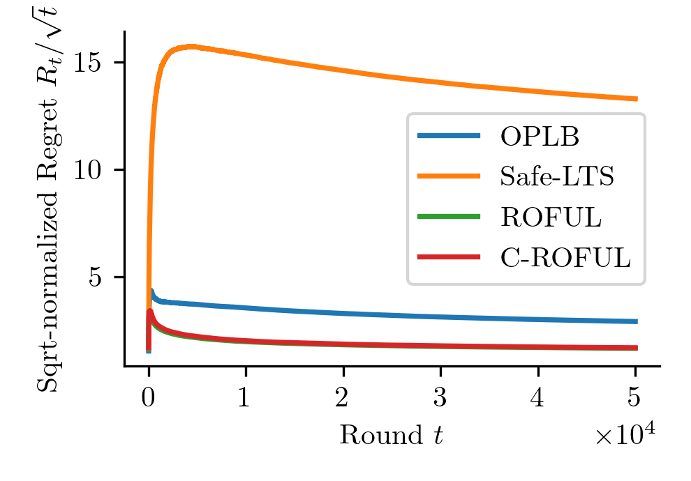
Figure 3: Simulation results for setting with linear constraints.

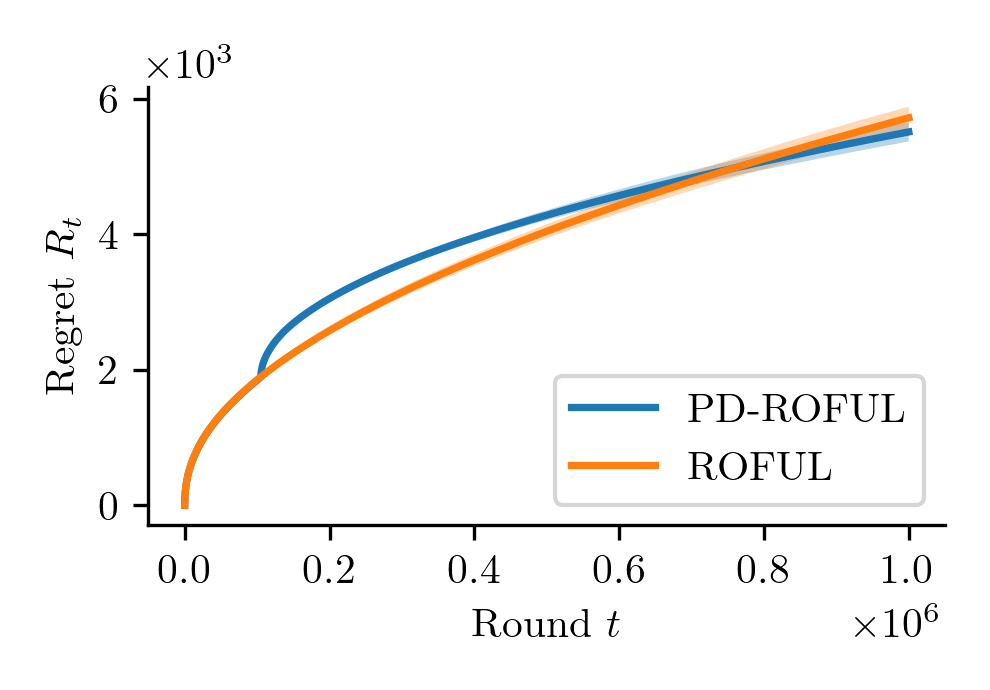
Figure 4: Simulation results for ROFUL and PD-ROFUL in problem with $\Delta>0$ and known.

In this section, we give the details of the numerical experiments that were not included in the body of the paper. We also include additional results.

G.1 Linear constraints

In this setting (results in Figure 2(a)), $d=2$, $\mathcal{X}=\mathbb{B}_{\infty}$ and $T=5\times 10^{4}$. For each trial, we sample parameters as $b\sim\mathcal{U}[0.25,1]$, $a\sim\mathcal{U}(\mathbb{B}_{\infty})$ and $\theta\sim\mathcal{U}(\mathbb{B}_{\infty})$. The learner is only given the prior information on these parameters that $\|\theta\|\leq\sqrt{2}$ and $\|a\|\leq\sqrt{2}$. As such, the algorithm can take $S_{a}=S_{\theta}=\sqrt{2}$. The noise terms are sampled i.i.d as $\eta_{t}\sim\mathcal{N}(\sigma)$ and $\epsilon_{t}\sim\mathcal{N}(\sigma)$, where $\sigma=0.1$. The learner is given $\sigma$. For the regularization parameter, we use $\lambda=1$ for all algorithms tested. Since all actions in the action set do not have norm less than $1$, we use a slightly large confidence set for all algorithms as specified by Theorem 2 in Abbasi-Yadkori et al. [2011] with $L=\sqrt{2}$. Note that the regret bounds of all algorithms will apply with a scaling of $L$.

We do not show the standard deviation in the results because it is too large to meaningful in the plot. The standard deviation is very large in this setting because the constraint may or may not be tight on the optimal action depending on the specific sampled problem.

Additional results

The experimental results for Safe-LTS are not included in the body because the regret is much larger than the regret of the other algorithms. We give the regret of all algorithms tested in Figure 3.

G.2 Linked convex constraints

In the first setting (results Figure 2(b)), $d=2$, $n=2$, $\mathcal{X}=\mathbb{B}$, and $T=10^{5}$. We take $\mathcal{G}=b\mathbb{B}$, where $b\sim\mathcal{U}[0.25,1]$ for each trial. The constraint matrix and reward vector are randomly sampled, where each row of $A$ is sampled as $a_{i}\sim\mathcal{U}(\mathbb{B}_{\infty})$ for all $i\in[n]$ and $\theta\sim\mathcal{U}(\mathbb{B}_{\infty})$. The learner is only given the prior information on these parameters that $\|\theta\|\leq\sqrt{2}$ and $\|a_{i}\|\leq\sqrt{2}$ for all $i\in[n]$. As such, the algorithms can take $S=\sqrt{2}$ and $r_{1}=0.25$. The noise terms are sampled i.i.d as $\eta_{t}\sim\mathcal{N}(\sigma I)$ and $\epsilon_{t}\sim\mathcal{N}(\sigma)$, where $\sigma=0.1$. The learner is given $\sigma$. For the regularization parameter, we use $\lambda=1$ for both algorithms. We simulate this setting for 30 trials, where different realizations of the problem parameters are used for each trial. In Figure 2(b), the mean of the regret at each round $t$ normalized by square-root $t$ is shown along with the plus-or-minus one standard deviation.

In the second setting (results Figure 2(c)), everything is the same except that $\mathcal{G}=b\mathbb{B}_{\infty}$ and $\mathcal{X}=\bigcup_{k\in[10]}\{\alpha u_{k}:\alpha\in[0,1]\}$ where $u_{k}\sim\mathcal{U}(\mathbb{S})$ for all $k\in[10]$. In Figure 2(c), the mean of the regret at each round $t$ normalized by square-root $t$ is shown along with plus-or-minus one standard deviation.

G.3 Finite star convex action set

In this setting (results in Figure 2(d)), the action set only consists of the coordinate directions with scalings between $0$ and $1$. We set $\theta=a=[1\ 0\ ...\ 0]^{\top}$ and $b=0.5$ and use i.i.d. Gaussian noise of standard deviation $0.1$. In this case, we only give the learner the knowledge that $\|a\|,\|\theta\|\leq S=2$ because if the learner was given the information that $\|a\|\leq 1$, it would be initially known that the optimal action satisfies the constraint. In this setting, we simulate ROFUL and Safe-PE for $3$ trials for each $d=10$.

Additional results

We also simulate PD-ROFUL (Algorithm 2) and ROFUL in the same setting with, except with $b=0.9$ and $S=1.5$. We make this modification to make the initial phase of duration less than $T$ so that there is a difference between ROFUL and PD-ROFUL. We simulate both algorithms for $5$ trials with $d=10$ and show the mean and standard deviation of the regret in Figure 4.

References

- Abbasi-Yadkori et al. [2011] Yasin Abbasi-Yadkori, Dávid Pál, and Csaba Szepesvári. Improved algorithms for linear stochastic bandits. Advances in neural information processing systems, 24, 2011.
- Achiam et al. [2017] Joshua Achiam, David Held, Aviv Tamar, and Pieter Abbeel. Constrained policy optimization. In International conference on machine learning, pages 22–31. PMLR, 2017.
- Agrawal and Devanur [2016] Shipra Agrawal and Nikhil Devanur. Linear contextual bandits with knapsacks. Advances in Neural Information Processing Systems, 29, 2016.
- Agrawal et al. [2016] Shipra Agrawal, Nikhil R Devanur, and Lihong Li. An efficient algorithm for contextual bandits with knapsacks, and an extension to concave objectives. In Conference on Learning Theory, pages 4–18. PMLR, 2016.
- Amani and Thrampoulidis [2021] Sanae Amani and Christos Thrampoulidis. Decentralized multi-agent linear bandits with safety constraints. In Proceedings of the AAAI Conference on Artificial Intelligence, volume 35, pages 6627–6635, 2021.
- Amani et al. [2019] Sanae Amani, Mahnoosh Alizadeh, and Christos Thrampoulidis. Linear stochastic bandits under safety constraints. Advances in Neural Information Processing Systems, 32, 2019.
- Amani et al. [2021] Sanae Amani, Christos Thrampoulidis, and Lin Yang. Safe reinforcement learning with linear function approximation. In International Conference on Machine Learning, pages 243–253. PMLR, 2021.
- Auer [2002] Peter Auer. Using confidence bounds for exploitation-exploration trade-offs. Journal of Machine Learning Research, 3(Nov):397–422, 2002.
- Badanidiyuru et al. [2013] Ashwinkumar Badanidiyuru, Robert Kleinberg, and Aleksandrs Slivkins. Bandits with knapsacks. In 2013 IEEE 54th Annual Symposium on Foundations of Computer Science, pages 207–216. IEEE, 2013.
- Badanidiyuru et al. [2014] Ashwinkumar Badanidiyuru, John Langford, and Aleksandrs Slivkins. Resourceful contextual bandits. In Conference on Learning Theory, pages 1109–1134. PMLR, 2014.
- Bura et al. [2022] Archana Bura, Aria HasanzadeZonuzy, Dileep Kalathil, Srinivas Shakkottai, and Jean-Francois Chamberland. Dope: Doubly optimistic and pessimistic exploration for safe reinforcement learning. Advances in Neural Information Processing Systems, 35:1047–1059, 2022.
- Cayci et al. [2020] Semih Cayci, Atilla Eryilmaz, and Rayadurgam Srikant. Budget-constrained bandits over general cost and reward distributions. In International Conference on Artificial Intelligence and Statistics, pages 4388–4398. PMLR, 2020.
- Chen et al. [2022a] Tianrui Chen, Aditya Gangrade, and Venkatesh Saligrama. A doubly optimistic strategy for safe linear bandits. arXiv preprint arXiv:2209.13694, 2022a.
- Chen et al. [2022b] Tianrui Chen, Aditya Gangrade, and Venkatesh Saligrama. Strategies for safe multi-armed bandits with logarithmic regret and risk. In International Conference on Machine Learning, pages 3123–3148. PMLR, 2022b.
- Chu et al. [2011] Wei Chu, Lihong Li, Lev Reyzin, and Robert Schapire. Contextual bandits with linear payoff functions. In Proceedings of the Fourteenth International Conference on Artificial Intelligence and Statistics, pages 208–214. JMLR Workshop and Conference Proceedings, 2011.
- Combes et al. [2015] Richard Combes, Chong Jiang, and Rayadurgam Srikant. Bandits with budgets: Regret lower bounds and optimal algorithms. ACM SIGMETRICS Performance Evaluation Review, 43(1):245–257, 2015.
- Dani et al. [2008] Varsha Dani, Thomas P Hayes, and Sham M Kakade. Stochastic linear optimization under bandit feedback. 2008.
- Fereydounian et al. [2020] Mohammad Fereydounian, Zebang Shen, Aryan Mokhtari, Amin Karbasi, and Hamed Hassani. Safe learning under uncertain objectives and constraints. arXiv preprint arXiv:2006.13326, 2020.
- Flaxman et al. [2005] Abraham D Flaxman, Adam Tauman Kalai, and H Brendan McMahan. Online convex optimization in the bandit setting: gradient descent without a gradient. In Proceedings of the sixteenth annual ACM-SIAM symposium on Discrete algorithms, pages 385–394, 2005.
- Grazzi et al. [2022] Riccardo Grazzi, Arya Akhavan, John IF Falk, Leonardo Cella, and Massimiliano Pontil. Group meritocratic fairness in linear contextual bandits. Advances in Neural Information Processing Systems, 35:24392–24404, 2022.
- Joseph et al. [2018] Matthew Joseph, Michael Kearns, Jamie Morgenstern, Seth Neel, and Aaron Roth. Meritocratic fairness for infinite and contextual bandits. In Proceedings of the 2018 AAAI/ACM Conference on AI, Ethics, and Society, pages 158–163, 2018.
- Kazerouni et al. [2017] Abbas Kazerouni, Mohammad Ghavamzadeh, Yasin Abbasi Yadkori, and Benjamin Van Roy. Conservative contextual linear bandits. Advances in Neural Information Processing Systems, 30, 2017.
- Khezeli and Bitar [2020] Kia Khezeli and Eilyan Bitar. Safe linear stochastic bandits. In Proceedings of the AAAI Conference on Artificial Intelligence, volume 34, pages 10202–10209, 2020.
- Kocák et al. [2020] Tomáš Kocák, Rémi Munos, Branislav Kveton, Shipra Agrawal, and Michal Valko. Spectral bandits. The Journal of Machine Learning Research, 21(1):9003–9046, 2020.
- Lattimore et al. [2020] Tor Lattimore, Csaba Szepesvari, and Gellert Weisz. Learning with good feature representations in bandits and in rl with a generative model. In International Conference on Machine Learning, pages 5662–5670. PMLR, 2020.
- Lindner et al. [2022] David Lindner, Sebastian Tschiatschek, Katja Hofmann, and Andreas Krause. Interactively learning preference constraints in linear bandits. In International Conference on Machine Learning, pages 13505–13527. PMLR, 2022.
- Liu et al. [2021a] Tao Liu, Ruida Zhou, Dileep Kalathil, Panganamala Kumar, and Chao Tian. Learning policies with zero or bounded constraint violation for constrained mdps. Advances in Neural Information Processing Systems, 34:17183–17193, 2021a.
- Liu et al. [2021b] Xin Liu, Bin Li, Pengyi Shi, and Lei Ying. An efficient pessimistic-optimistic algorithm for stochastic linear bandits with general constraints. Advances in Neural Information Processing Systems, 34:24075–24086, 2021b.
- Moradipari et al. [2020] Ahmadreza Moradipari, Christos Thrampoulidis, and Mahnoosh Alizadeh. Stage-wise conservative linear bandits. Advances in neural information processing systems, 33:11191–11201, 2020.
- Moradipari et al. [2021] Ahmadreza Moradipari, Sanae Amani, Mahnoosh Alizadeh, and Christos Thrampoulidis. Safe linear thompson sampling with side information. IEEE Transactions on Signal Processing, 69:3755–3767, 2021.
- Pacchiano et al. [2021] Aldo Pacchiano, Mohammad Ghavamzadeh, Peter Bartlett, and Heinrich Jiang. Stochastic bandits with linear constraints. In International conference on artificial intelligence and statistics, pages 2827–2835. PMLR, 2021.
- Rusmevichientong and Tsitsiklis [2010] Paat Rusmevichientong and John N Tsitsiklis. Linearly parameterized bandits. Mathematics of Operations Research, 35(2):395–411, 2010.
- Sui et al. [2015] Yanan Sui, Alkis Gotovos, Joel Burdick, and Andreas Krause. Safe exploration for optimization with gaussian processes. In International conference on machine learning, pages 997–1005. PMLR, 2015.
- Sui et al. [2018] Yanan Sui, Vincent Zhuang, Joel Burdick, and Yisong Yue. Stagewise safe bayesian optimization with gaussian processes. In International conference on machine learning, pages 4781–4789. PMLR, 2018.
- Usmanova et al. [2019] Ilnura Usmanova, Andreas Krause, and Maryam Kamgarpour. Safe convex learning under uncertain constraints. In The 22nd International Conference on Artificial Intelligence and Statistics, pages 2106–2114. PMLR, 2019.
- Valko et al. [2014] Michal Valko, Rémi Munos, Branislav Kveton, and Tomáš Kocák. Spectral bandits for smooth graph functions. In International Conference on Machine Learning, pages 46–54. PMLR, 2014.
- Varma et al. [2023] K Nithin Varma, Sahin Lale, and Anima Anandkumar. Stochastic linear bandits with unknown safety constraints and local feedback. In ICML Workshop on New Frontiers in Learning, Control, and Dynamical Systems, 2023.
- Wachi and Sui [2020] Akifumi Wachi and Yanan Sui. Safe reinforcement learning in constrained markov decision processes. In International Conference on Machine Learning, pages 9797–9806. PMLR, 2020.
- Wan et al. [2022] Runzhe Wan, Branislav Kveton, and Rui Song. Safe exploration for efficient policy evaluation and comparison. In International Conference on Machine Learning, pages 22491–22511. PMLR, 2022.
- Wang et al. [2022] Zhenlin Wang, Andrew J Wagenmaker, and Kevin Jamieson. Best arm identification with safety constraints. In International Conference on Artificial Intelligence and Statistics, pages 9114–9146. PMLR, 2022.
- Wu et al. [2015] Huasen Wu, Rayadurgam Srikant, Xin Liu, and Chong Jiang. Algorithms with logarithmic or sublinear regret for constrained contextual bandits. Advances in Neural Information Processing Systems, 28, 2015.
- Wu et al. [2016] Yifan Wu, Roshan Shariff, Tor Lattimore, and Csaba Szepesvári. Conservative bandits. In International Conference on Machine Learning, pages 1254–1262. PMLR, 2016.