Generative Model for Models: Rapid DNN Customization for Diverse Tasks and Resource Constraints

Abstract.

Unlike cloud-based deep learning models that are often large and uniform, edge-deployed models usually demand customization for domain-specific tasks and resource-limited environments. Such customization processes can be costly and time-consuming due to the diversity of edge scenarios and the training load for each scenario. Although various approaches have been proposed for rapid resource-oriented customization and task-oriented customization respectively, achieving both of them at the same time is challenging. Drawing inspiration from the generative AI and the modular composability of neural networks, we introduce NN-Factory, an one-for-all framework to generate customized lightweight models for diverse edge scenarios. The key idea is to use a generative model to directly produce the customized models, instead of training them. The main components of NN-Factory include a modular supernet with pretrained modules that can be conditionally activated to accomplish different tasks and a generative module assembler that manipulate the modules according to task and sparsity requirements. Given an edge scenario, NN-Factory can efficiently customize a compact model specialized in the edge task while satisfying the edge resource constraints by searching for the optimal strategy to assemble the modules. Based on experiments on image classification and object detection tasks with different edge devices, NN-Factory is able to generate high-quality task- and resource-specific models within few seconds, faster than conventional model customization approaches by orders of magnitude.

1. Introduction

Deep learning (DL) has become a game-changing artificial intelligence (AI) technology in recent years. It has achieved remarkable performance in various domains including computer vision, natural language understanding, computer gaming, and computational biology. Meanwhile, deep learning has enabled and enhanced many intelligent applications at the edge, such as driving assistance (He et al., 2021; Zhang et al., 2021b), face authentication (Chen et al., 2017), video surveillance (Zhang et al., 2021c; Jiang et al., 2021), speech recognition (Wang et al., 2020; Park et al., 2018), etc. Due to latency and privacy considerations, it is becoming an increasingly common practice to deploy the models to edge devices (Liu et al., 2020; Guo et al., 2021; Kong et al., 2023), so that the models can be directly invoked without transmitting data to the server.

To adopt DL models in different edge scenarios, developers usually need to customize the models, which includes the following two main processes.

1. Task-oriented Customization: Customizing the models for domain-specific tasks, such as detecting certain types of cars, tracking people with certain costume, or identifying items with certain failures.

2. Resource-oriented Customization: Customizing the models for edge devices, in order to fulfill certain resource constraints on the target edge device, including the memory budget and the latency requirement.

The current practice is to deal with each customization problems separately. For example, developers need to generate compact models through extensive model architecture designing/compression to meet the resource constraints, and then train/fine-tune the model on the domain-specific tasks to improve accuracy. Such a process may involve expensive data collection, time-consuming architecture search, and unstable model training.

Recent advances of deep learning have demonstrated excellent zero-shot adaptation abilities of large pretrained models, including training-free neural architecture adaptation and task adaptation. Specifically, one-shot neural architecture search (NAS) (Cai et al., 2020a; Cai et al., 2019) and model scaling (Han et al., 2021; Fang et al., 2018; Wen et al., 2023; Jeon et al., 2023) techniques have demonstrated the possibility of training a supernet and customizing it for diverse edge environments. Pretrained large models like ChatGPT (OpenAI, 2022), OFA (Cai et al., 2020b), and Segment Anything (Chowdhery et al., 2022) allow users to customize the task of the model by simply providing a task prompt as the model input. Such training-free adaptation abilities are desirable in edge AI scenarios due to the possibility to support a wide range of downstream tasks and diverse hardware constraints with significantly reduced development efforts.

However, it is difficult to combine training-free neural architecture customization and training-free task customization together. On one hand, using one-shot NAS or model scaling to generate models for different tasks is not feasible since the supernet is designed for a single task. Extending them to multiple tasks would significantly enlarge the model search space, making the supernet training and subnet search extremely challenging. On the other hand, the remarkable task adaptation abilities of pretrained models come at the cost of huge computational load. Recent studies have shown that the zero-shot generalization ability of pretrained models emerges and strengthens with increasing model size (Kaplan et al., 2020). Thus, it is difficult or even impossible to directly use the task-generalizable large model due to the diverse and limited edge computational resources.

To achieve both task-oriented and resource-oriented efficient model customization, we introduce NN-Factory, a new paradigm for generating customized models for diverse edge scenarios. Our key idea is to view the problem of edge-specific model customization as a generative problem - rather than existing generative models that are designed for generating media content (OpenAI, 2022; Creswell et al., 2018; Croitoru et al., 2023), we use generative AI to produce customized models based on edge scenario specifications. Specifically, given the desired task, the device type, and the resource requirements in an edge scenario, NN-Factory rapidly produces a compact model that matches the task and requirements by simply querying the generative model. Such a new paradigm of model customization has the potential to fundamentally avoid the cumbersome compression and training processes in conventional edge model customization approaches.

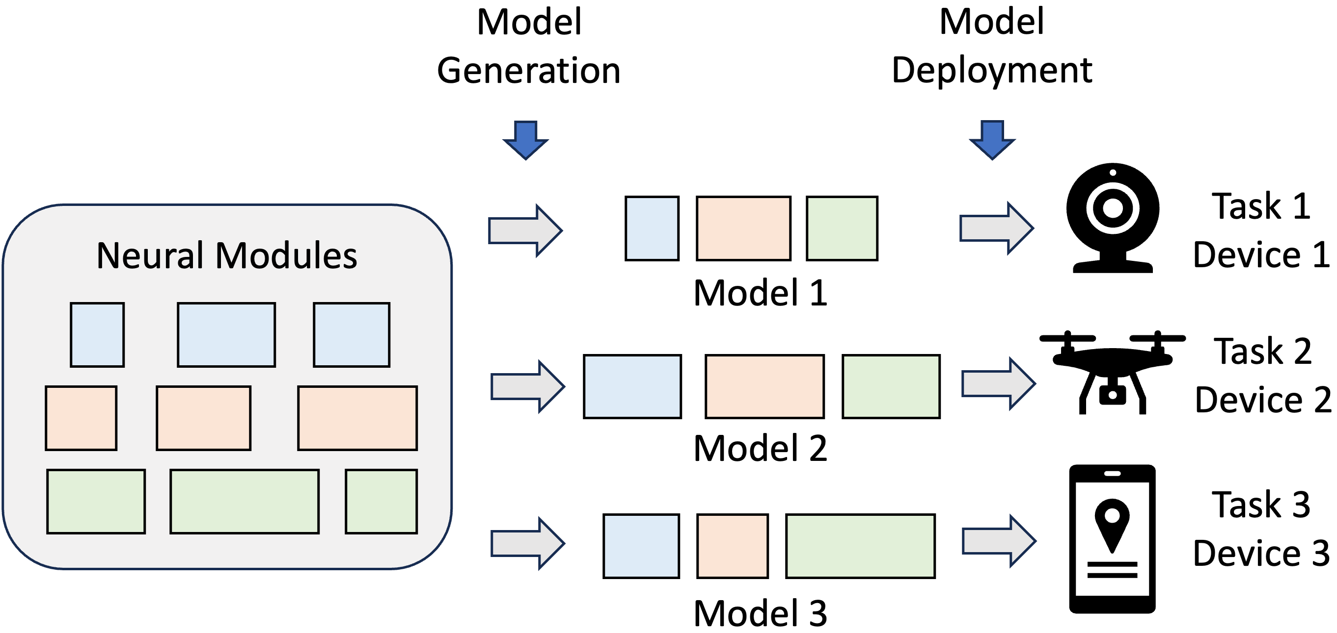
Figure 1. The key idea of NN-Factory: Generating models for diverse edge scenarios by assembling modules.

However, directly generating the parameters of a model is difficult due to the enormous number of model parameters. The key insight of NN-Factory to address this problem is the composability of neural network modules (Andreas et al., 2016; Parisotto et al., 2016), i.e. different functionalities and sizes of neural networks can be achieved by certain combinations of neural network modules, as illustrated in Figure 1. Such modular composability has been studied by existing approaches (e.g. NestDNN (Fang et al., 2018), LegoDNN (Han et al., 2021), AdaptiveNet (Wen et al., 2023), etc.) for edge-side model scaling, but none of them is able to support task-oriented customization.

Based on this insight, NN-Factory generates a customized model for each edge scenario by directly generating the configurations to assemble pretrained neural modules. The key components of NN-Factory include a modular supernet that carries the neural modules, a task- and sparsity-aware module assembler that generates candidate module assembling configurations (each configuration is a set of gate vectors that can map to a candidate model), and a lightweight architecture searcher that rapidly finds the optimal configuration to assemble the model for the target edge scenario.

Specifically, the modular supernet is extended from a common backbone network, such as Convolutional Neural Network (CNN) or Transformer, in which each basic block is decomposed to multiple conditionally activated modules. How the modules are activated is controlled by several gate vectors, which are produced by a generative model (i.e. the module assembler). By activating different sets of modules, the basic blocks in the backbone network can be reconfigured to have different functionalities and sizes. The module assembler decides how to activate the modules in the backbone network based on a task description and a sparsity requirement (i.e. a limit of module activation ratio). The modules and assembler are jointly trained to coherently work together.

Based on the module-assembler design, we are able to reduce the large search space of module combinations to a small search space of generation prompts. To find the customized model for an edge scenario (defined by the task, device, and latency/memory requirements), we only need to find the optimal model generation request, which is done by the lightweight architecture search module under the guidance of a device-specific model performance evaluator. Due to the significantly reduced search space, finding the optimal model only takes few short iterations.

To evaluate NN-Factory, we conduct experiments with three devices on two types of tasks. The results have demonstrated that our approach can generate tailored models for a given edge scenario in up to 6 seconds, 1000$\times$ faster than the conventional training-based customization approach. The generated models can achieve high accuracy that is comparable with edge retrained/fine-tuned models on both known and unseen tasks.

Our work makes the following technical contributions:

1. We propose a novel generative AI-based edge-specific model customization solution. It enables rapid training-free model customization for edge scenarios with diverse tasks and resource constraints.

2. We introduce a modular design for model generation, which enables rapid model customization by simply querying an assembler model for module activations.

3. Based on experiments with two types of tasks and various edge devices, our method is able to generate high-quality models for diverse edge scenarios with significantly lower overhead. The system and models will be open-sourced.

2. Background and Related Work

2.1. Model Customization for Edge Scenarios

Deploying deep neural networks (DNNs) at the edge is increasingly popular due to the latency requirements and privacy concerns of deep learning services. However, directly following the common cloud-based model training and deployment procedures is not satisfactory due to the huge diversity of edge scenarios (Wen et al., 2023; Han et al., 2021; Fang et al., 2018). Unlike most cloud-based AI models that are designed for generic tasks and hosted in powerful GPU clusters, edge AI scenarios are usually diverse and fragmented. Each edge scenario may deal with a domain-specific task and a unique set of target deployment environments.

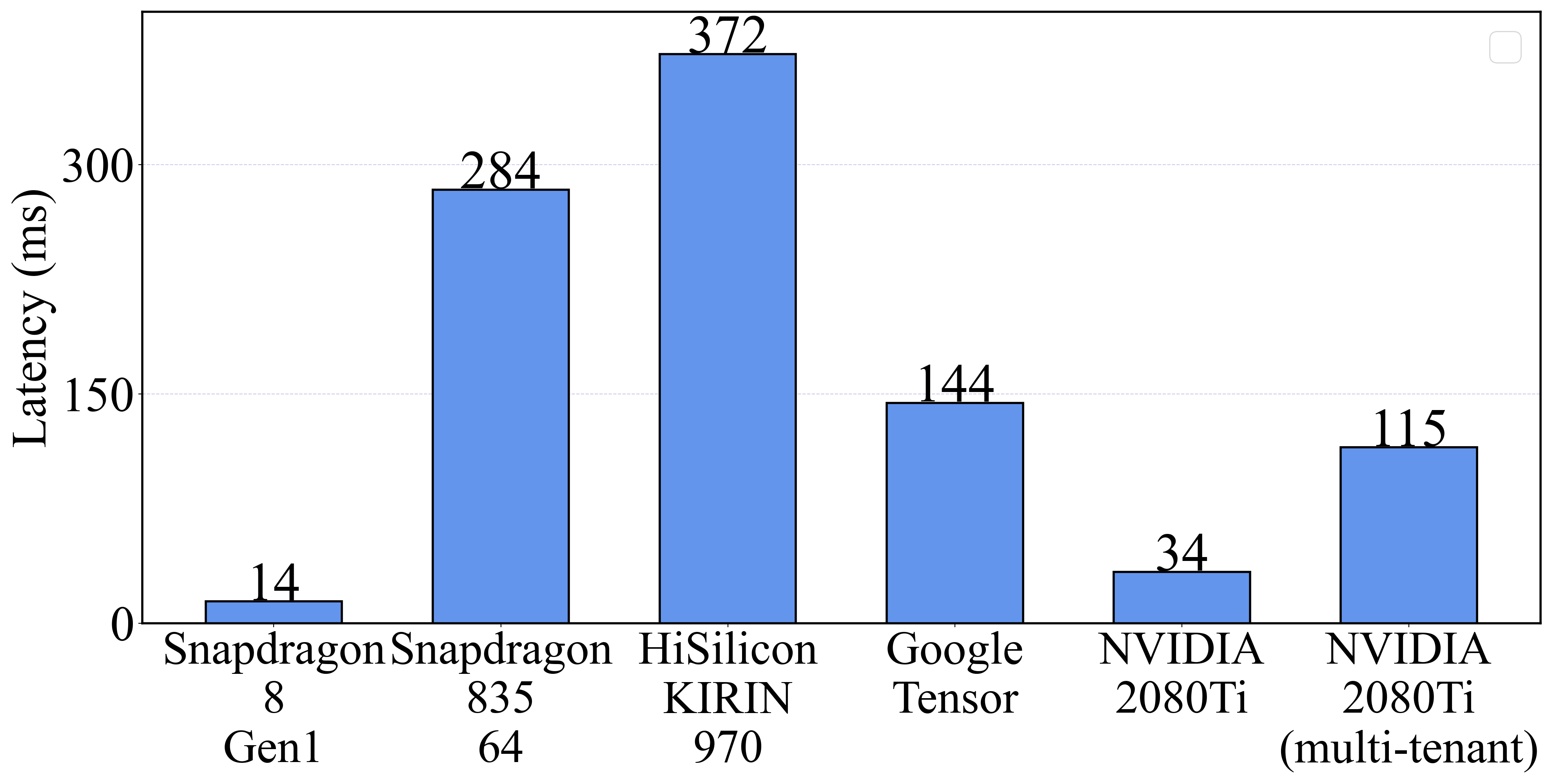
Figure 2. Average latency (ms) of ResNet50 in different deployment environments. In the “multi-tenant” setting, we assume there are three background processes running the same model.

Table 1. Typical AI tasks requested by the customers of an edge AI service provider.

Customer	Task
Construction site	Detect people wearing blue uniform.
Restaurant	Classify people wearing white chef cap.
Hospital	Classify people wearing masks.
Shopping mall	Detect smoking people.
Traffic station	Detect cars with green plates.

According to our industry partners that provide edge AI services for the customizers, their major development efforts are spent on customizing models to handle the diversities of edge scenarios, including hardware diversity, task diversity, data distribution diversity, etc. Among them, a major problem is the hardware diversity. Customizers usually require to deploy models to different hardware platforms, such as edge servers, desktops, smartphones, and edge AI boxes. Due to the different computational capabilities, the same model may yield significantly different performances on different edge devices and environments, as shown in Figure 2. Therefore, developers need to customize the model architectures to meet the latency constraints. Task diversity is another important problem faced by edge AI service providers. Each customizer may have a domain-specific AI task based on the application scenario, as illustrated in Table 1. To enable AI services in such scenarios, customizing the model for the different tasks is necessary.

There are various existing approaches proposed for each type of the above customization goals. However, when considering the two goals jointly for many diverse edge scenarios, the cost becomes huge, since the customization process is non-trivial (as will be explained later) and has to be repeated for each scenario.

2.2. Training-based Model Customization

To customize a model for a certain domain-specific task, the common practice is to use transfer learning (TL). The predominant approach in transfer learning is is fine-tuning, i.e. initializing the model parameters with a pretrained model and continue training the parameters with domain-specific data. Such transfer learning processes require developers to collect data samples for the task, label them, and train the model with the labeled samples, which are usually labor-intensive, resource-demanding, and time-consuming.

To fit a model into a specific edge device, the typical solutions include compressing an existing model (Han et al., 2016; Wang et al., 2019; Zhu et al., 2020) (e.g. pruning, quantization, etc.) or finding a new model architecture that aligns with the capabilities of the target device (Sandler et al., 2018; Tan and Le, 2021). Since manually designing models for diverse edge environments is cumbersome, the common practice is to use automated model generation techniques. NAS (Tan et al., 2019a; Guo et al., 2020; Wu et al., 2019; Yang et al., 2018; Li et al., 2020) is the most representative and widely-used model generation method, which searches for the optimal network architecture in a well-designed search space. Most NAS methods require training the architectures during searching (Zoph and Le, 2016; Real et al., 2019; Tan et al., 2019a; Liu et al., 2018), which is exceedingly time-consuming (10,000+ GPU hours) when generating models for a large number of devices.

Both of the above processes pose challenges for developers due to the diversity of edge scenarios. Training or fine-tuning the model for one edge scenario typically requires thousands of labeled training samples and several hours on high-performance GPU machines. Finding the optimal model architecture or compression strategy by trial and error also requires much development effort.

2.3. Training-free Model Customization

The recent advances of deep learning have shown the feasibility to use a unified pretrained model to support various downstream tasks without further training. Specifically, one can train a foundation model on a large dataset with various predefined tasks and directly use the model for different downstream tasks with simple prompts. According to empirical analyses (Kaplan et al., 2020), improving the capacity of pretrained model can lead to better performance on downstream tasks.

Meanwhile, both the AI community and the mobile computing community have attempted various ways to reduce the cost of generating lightweight models for edge devices. One-shot NAS (Cai et al., 2019; Cai et al., 2020a; Liu et al., 2021; Huang and Chu, 2021) is proposed to greatly reduce the training cost by allowing the candidate networks to share a common over-parameterized supernet. The best models for the target device can be found by directly searching a subnet in the supernet. Mobile computing researchers have also proposed to scale models dynamically to provide a wide range of resource-accuracy trade-offs. Most of them apply structured pruning or model architecture adaptation to generate descendent models (Fang et al., 2018; Yu et al., 2018; Yu and Huang, 2019; Han et al., 2021; Liu et al., 2017) with different levels of computational cost.

Training-free model adaptation can also be achieved by dynamically assembling neural modules, which have been discussed in dynamic neural networks (Han et al., 2022) and neurosymbolic programming (Parisotto et al., 2016). Dynamic neural networks are a type of DNNs that support flexible inference based on the difficulty of input. When the input is easy, dynamic neural networks can reduce the computation by skipping a set of blocks (Wang et al., 2018; Wu et al., 2018) or exiting from the middle layers (Bolukbasi et al., 2017; Laskaridis et al., 2020; Laskaridis et al., 2021; Fang et al., 2020). Although different subnets (a subnet is a path in the dynamic NN) have different computational load, they cannot be customized for different tasks, and the input-dependent model dynamicality is also not suitable for edge environments. Neurosymbolic programming demonstrates the possibility to solve different tasks with a same set of neural modules by semantically combining them. Specifically, the model to solve a complex task can be written as a program that invokes smaller function modules. However, existing neurosymbolic programming approaches are short of flexibility and resource-oriented customization ability, because the modules are usually static and explicitly defined.

However, it remains challenging to optimize the model customization process for tasks and devices at the same time. The task-oriented customization and the resource-oriented customization are somewhat conflicting. To achieve fast task customization, the model is desired to have cross-task generalization ability, which typically requires a unified pretrained model with large capability, while deploying the model to diverse resource-limited edge devices requires non-uniform lightweight models.

3. NN-Factory Design

Problem definition. Formally, the goal of edge DNN customization is to generate a model $f_{\hat{\alpha},\hat{\theta}}$ with architecture $\hat{\alpha}$ and parameters $\hat{\theta}$ that can accurately handle the edge task while satisfying the performance constraints. i.e.

(1) $$\begin{split}\hat{\alpha},\hat{\theta}=\>&\arg\min_{\alpha,\theta}\>{L(f_{\alpha,\theta}(X^{e}),Y^{e})}\\ &s.t.\>mem(\alpha)<MEM^{e}\>and\>lat(\alpha)<LAT^{e}\end{split}$$

where $X^{e}$ and $Y^{e}$ are the input and output of edge task data samples, $L$ is the prediction loss, and $MEM^{e}$ and $LAT^{e}$ are the memory and latency limits at the edge environment.

Specifically, we focus on generating models for the tasks in a combinatorial space, i.e. each task is described as a combination of several properties (e.g. color, status, entity, etc.) and the properties are shared across different tasks (e.g. red truck, white cat, etc.). Developers can flexibly define the task space according to their target edge scenarios.

Our work takes inspiration from the modularity and dynamic composability of neural networks and generative AI. Our vision is to create an one-for-all generative system in which different edge-specific DNN models can be directly generated by configuring and assembling predefined neural modules, as illustrated in Figure 1.

Realizing this vision is challenging because (1) it is hard to design and develop the modules that can be assembled to do different tasks and fulfill different resource constraints (2) even if such modules are created, generating a tailored model for a specific edge scenario may still be difficult due to the huge combinational space of model candidates.

We attempt to address these challenges with an end-to-end approach named NN-Factory. We highlight that NN-Factory is a first-of-its-kind generative paradigm of model customization for diverse edge scenarios, which enables rapid training-free model generation for different tasks and resource constraints.

3.1. Overview

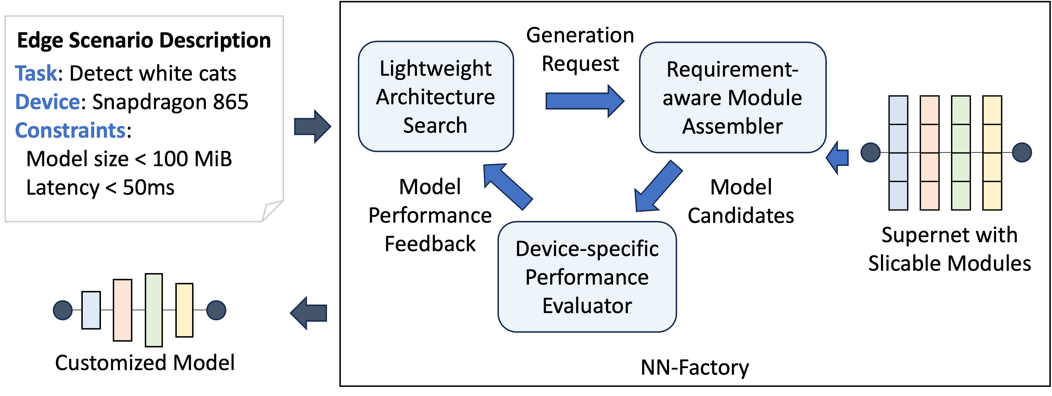
Figure 3. Architecture overview of NN-Factory.

The main idea of NN-Factory is to jointly train a set of neural modules and a module assembling strategy generator (i.e. assembler) in a task- and sparsity-grounded manner. Specifically, the modules are sliced from a pretrained neural network (supernet), which avoids the cumbersome development of individual modules with the cost of limited interpretability. Meanwhile, by learning the assembler during training with many different tasks and sparsity requirements, NN-Factory can directly produce the model architecture for a new task and sparsity requirement with a single forwarding pass, significantly reducing the model search space.

Figure 3 shows the overview of NN-Factory. It contains three main components, including a supernet with sliceable modules, a requirement-aware assembler, and a lightweight architecture search module. and a device-specific edge performance evaluator. The supernet contains the basic modules that can be flexibly combined to form customized models (subnets). The requirement-aware module assembler is a generative model that produces module assembling configurations based on the given task and sparsity requirements. Each generated configuration maps to a model candidate. The lightweight architecture search module finds the optimal model by iteratively searching and evaluating model candidates according to an edge-specific performance evaluator.

Given an edge scenario (described by the task, device type, and resource constraints), the model customization workflow of NN-Factory is consist of the following steps:

1. The lightweight architecture search module proposes a model generation request ¡task, activation limit¿, where activation limit is the maximum ratio of activated modules in the model.

2. The requirement-aware assembler predicts a module assembling configuration based on the request. The configuration describes how to produce a candidate model by activating and assembling the modules in the supernet.

3. The device-specific performance evaluator evaluates the generated configuration (i.e. the candidate model) against the edge resource constraints. If the constraints are satisfied and the memory/latency budget is fully utilized, then return the current candidate. Otherwise, go back to step (1) with a new generation request.

The following subsections will introduce the main components in more detail.

3.2. Supernet with Slicable Modules

The supernet is responsible for providing the basic neural modules that can be reassembled to fulfill different tasks and resource constraints. Slicing an existing neural network for different function blocks for interpretability has been studied before (Zhang et al., 2020; Zhang et al., 2022; Zhang et al., 2023), but the sliced modules are usually coarse-grained and difficult to reassemble. We decide to directly train a slicable supernet for better modular separation and composability.

We build the modular supernet by extending an existing backbone network. The backbone network extracts features from given inputs and make the final predictions. We are able to support common backbones based on Convolution Neural Networks (CNNs) and Transformers, such as ResNet (He et al., 2016), EifficentNet (Tan and Le, 2019), and Vision Transformer (Dosovitskiy et al., 2020).

CNN Backbone. First, we introduce how to convert a convolutional layer in the CNN architecture to slicable modules. Given a feature map $x$ as a input, the output of $l$-th convolutional layer is $O^{l}(x)$. In a conventional CNN, $O^{l}(x)$ is computed as:

(2) $$O_{i}^{l}=\sigma(F_{i}^{l}*I^{l}(x))$$

where $O_{i}^{l}$ is the $i$-th channel of $O^{l}(x)$ , $F_{i}^{l}$ is the $i$-th filter, $\sigma(\cdot)$ denotes the element-wise nonlinear activation function and $*$ denotes convolution. the output feature map $O^{l}(x)$ is obtained by applying all the filters $F_{i}^{l}$ in the current layer to the input feature map $I^{l}(x)$.

In NN-Factory, we treat each convolutional filter as a module that can be conditionally activated. By activating different combinations of filters in a convolution layer, the resulting layers can deemed to have different functionalities.

Based on such modular decomposition, we introduce a gate vector $g$ to control the activation of the modules. With the gate vector, the computation of feature map $O_{i}^{l}$ in Equation 2 is reformulated as below:

(3) $$O_{i}^{l}=\sigma(F_{i}^{l}*I^{l}(x))\cdot g_{i}^{l}$$

where $g_{i}^{l}$ is the entry in $g$ corresponding to the $i$-th filter at layer $l$ and 0 is a 2-D feature map with all its elements being 0, only when $g_{i}^{l}$ equals to 1, the $i$-th filter will be applied to $I^{l}$ to extract features. Figure 4 depicts the computation process as described above.

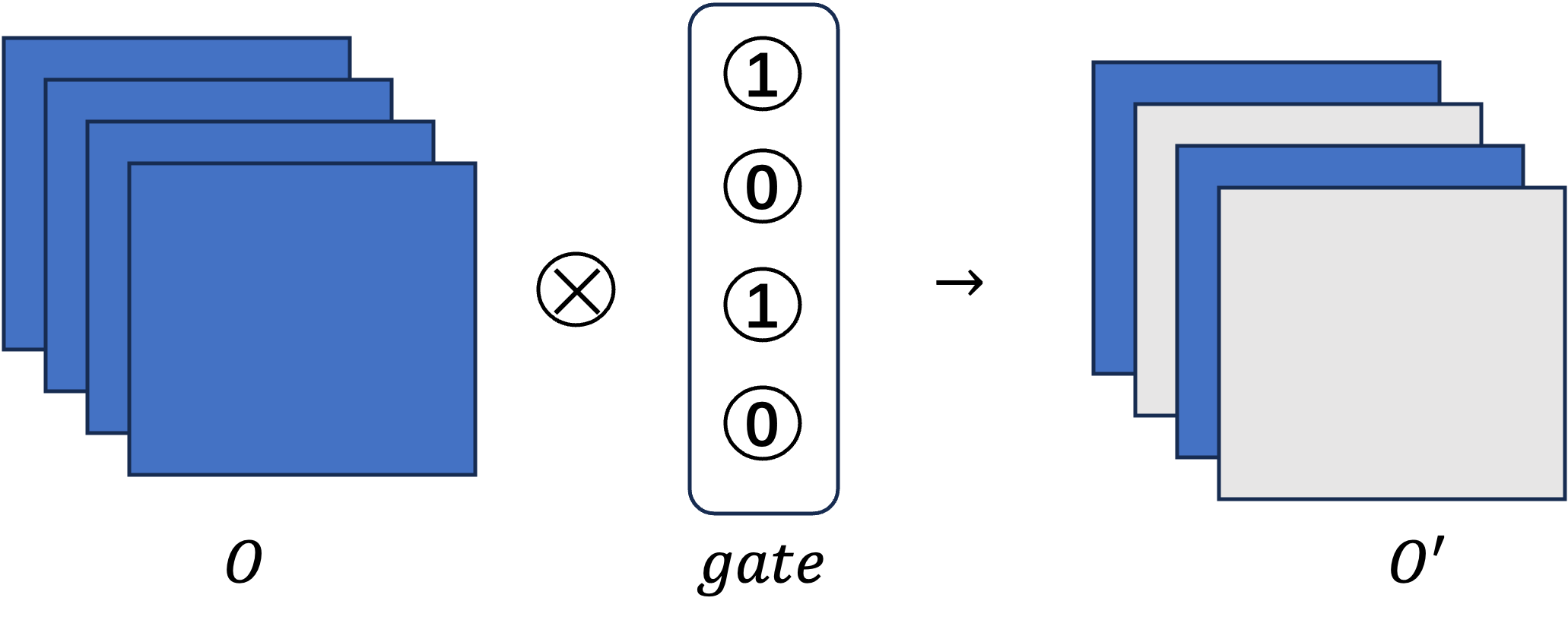
Figure 4. An illustration of modular convlutional layer with conditionally-activated convolution filters. $O$ represents the output feature map of a convolutional layer with four channels. Each element in the gate vector maps to a channel. By applying different gate vectors, different combinations of the filters are activated.

The modular supernet is obtained by applying the modularization process to the main convolution layers in the CNN model. The batch normalization layer after each convolution layer is sliced in a channel-wise manner and controlled by the same gate vector. It is worth noting that, in modern deep CNN architectures such as ResNet, EfficientNet, and MobileNet, the convolutional layers are organized as several basic blocks. We do not convert the convolutional layers at the end of each basic block in order to avoid shape conflicts with the residual connections. Figure 6(a) and (b) illustrate the common CNN basic blocks that are integrated with learnable module gates.

Transformer backbone. We also support generating modular supernets from Transformer backbones. The main components of Transformer include self-attention layers and feed-forward networks (FFNs). According to recent studies (Dai et al., 2021), the FFN components store various factual knowledge learned from data. A FFN is a two-layer fully connected networks, which process an input representation $x\in\mathbb{R}^{dmodel}$ as:

(4) $$h =xW_{1}$$

$$F(x) =\sigma(h)W_{2}$$

where $W_{1}\in\mathbb{R}^{dmodel\times dff}$ and $W_{2}\in\mathbb{R}^{dff\times dmodel}$ are the weight matrices.

The Transformer architecture is not modular by design, but it can be converted into an equivalent Mixture-of-Experts (MoE) model (Jacobs et al., 1991; Zhang et al., 2021a), in which each expert can be regarded as a conditionally-activated function module. Inspired by this idea, we propose to modularize the FFN layers in Transformer backbones and reformulate the computation of $F(x)$ in Equation 4 as below:

(5) $$h =xW_{1}$$

$$h^{{}^{\prime}} =h\cdot g_{FFN}$$

$$F(x) =\sigma(h^{{}^{\prime}})W_{2}$$

where $g_{FFN}$ represents the gate selection for the current FFN layer. If the $i$-th position in $g_{FFN}$ is 0, the corresponding position in $h^{\prime}$ is set to 0 as well, indicating that the parameters in the corresponding parts of $W_{1}$ and $W_{2}$ are not activated.In Figure  5, we demonstrate the parameters that remain inactive under the gate’s selection.

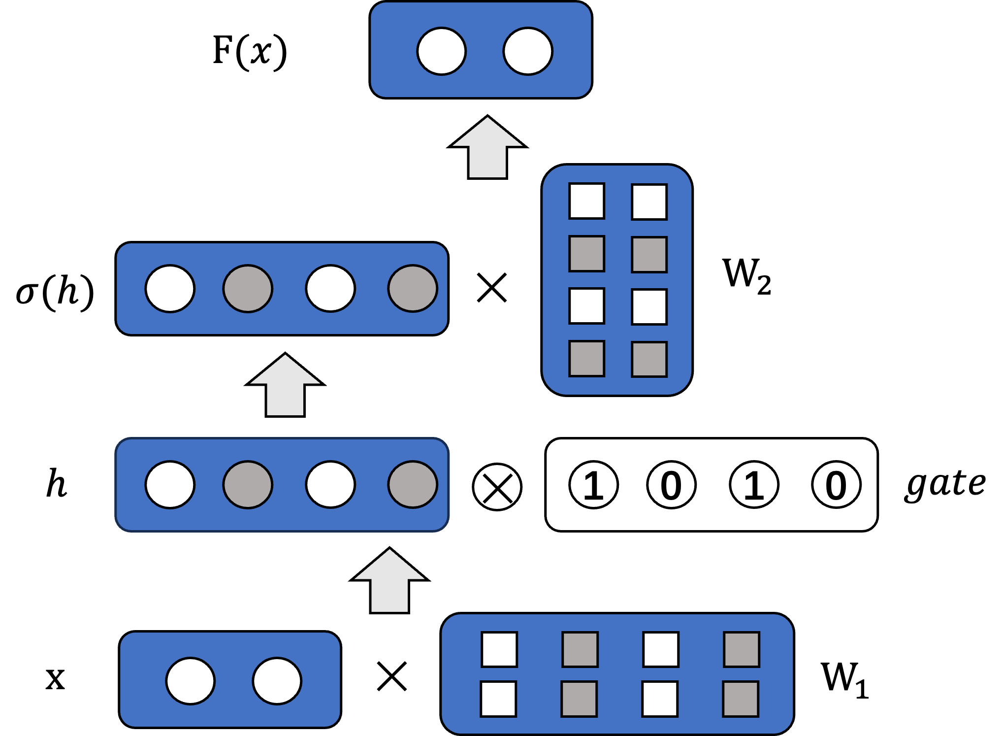
Figure 5. An illustration of modular FFN layer in Transformer backbones. The intermediate feature $h$ of FFN is conditionally activated along the hidden dimension. Each element in the gate vector maps to a element in $h$. According to the activation of $h$, the corresponding dimensions in $W_{1}$ and $W_{2}$ can be selectively pruned.

Similarly, by applying the modularization process to all FFNs in a Transformer backbone, we can obtain a Transformer-based supernet for NN-Factory, an illustration with the ViT backbone is shown in Figure 6(c).

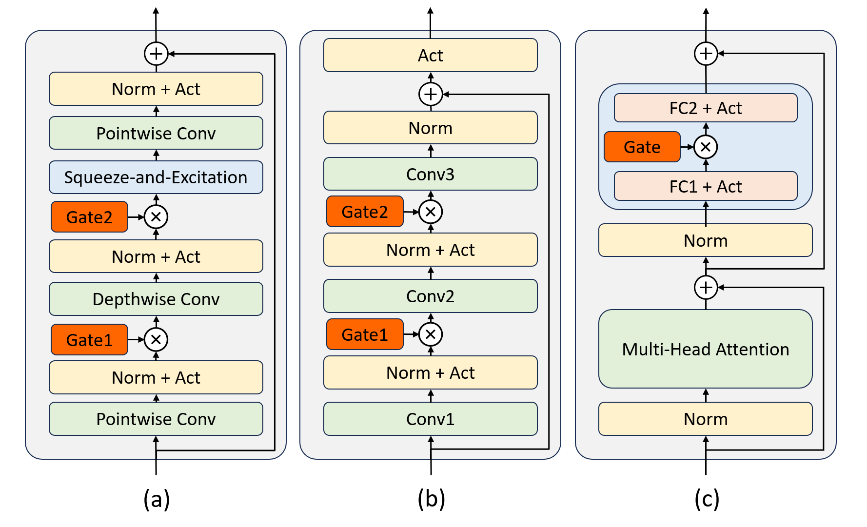
Figure 6. Gate integration for the different backbones. (a) EfficientNet and MobileNet. (b) ResNet. (c) ViT.

3.3. Requirement-aware Module Assembler

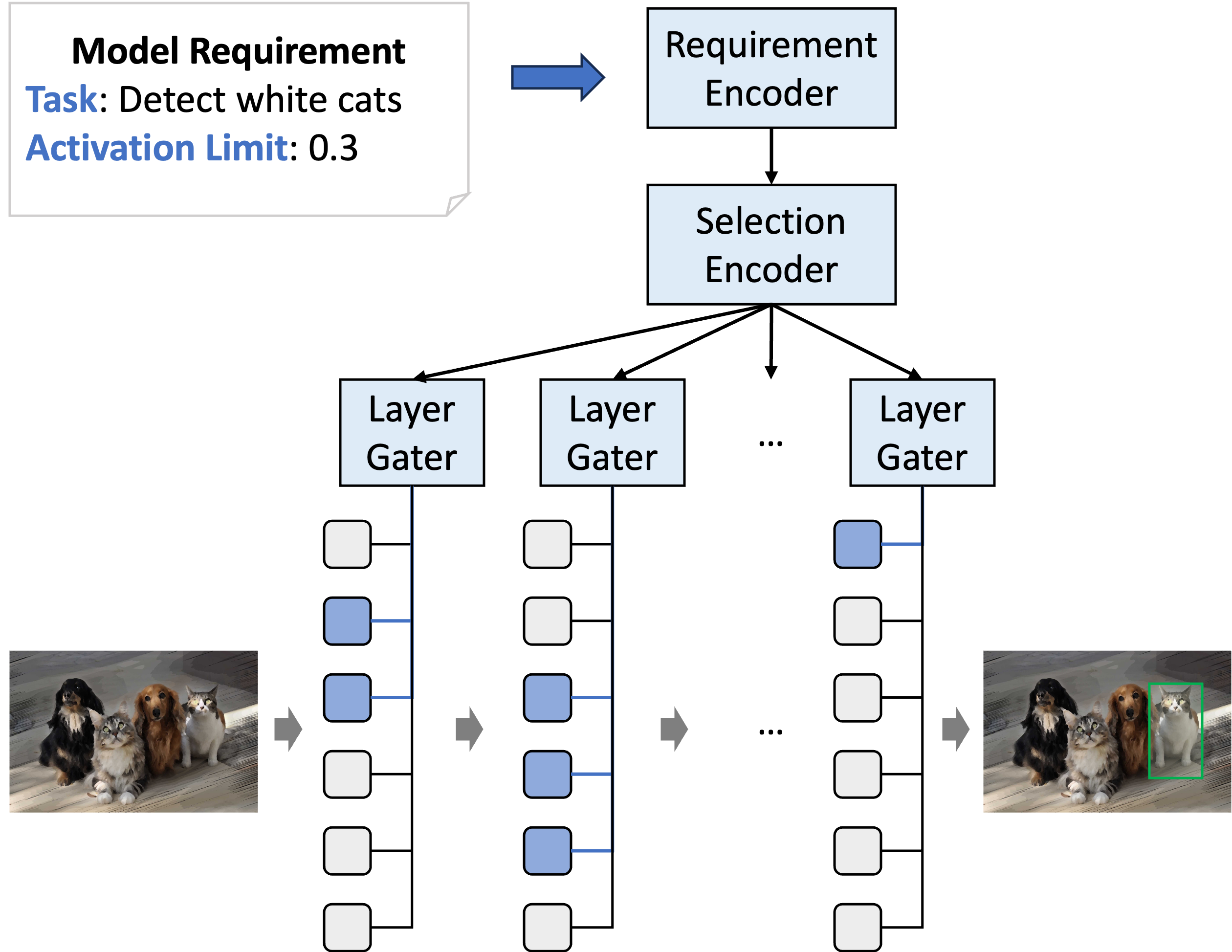
Figure 7. Architecture of the requirment-aware module assembler, integrated with the modular backbone.

The module assembler plays a vital role in NN-Factory- it generates gate vectors that controls the activations of neural modules in the supernet, such that the activated modules can be assembled to produce a candidate model.

The input of the module assembler is a model generation request, represented as a tuple ¡$task$, $activation\_limit$¿. $task$ is a description of the target task in the edge scenario. As mentioned in Section 3, a task can be represented as a combination of several properties. For example, the task ‘detect black dogs’ is represented as $\{black,dog\}$ and ‘detect white cat’ is $\{white,cat\}$. $activation\ limit$ is a sparsity requirement that regulates the ratio of activated modules in the generated model. A lower limit will encourage the assembler to generate smaller candidate models.

The output of the assembler is the gate vectors $g$ as described in Section 3.2. Each gate vector $g_{l}$ corresponds to a modular layer $l$ in the supernet and determines the activations of the modules in the layer.

The network architecture of the assembler is shown in Figure 7. It consists of three main components, including a requirement encoder, a selection encoder, and a list of layer gaters. The requirement encoder transforms the description of task and sparsity requirement $activation\_limit$ into an embedding. We use the one-hot encoding for the $task$ component, denoted by $enc_{task}$. Each bit in $enc_{task}$ represents the presence of a specific property. For example, in the task ‘detect black dog’, the elements for ‘black’ and ‘dog’ are set to one and others are set to zero in the task encoding. Regarding the $activation\_limit$ component, we utilize Positional Encoding (Vaswani et al., 2017) to encode the limit ratio, denoted by $enc_{limit}$. The two encodings $enc_{task}$ and $enc_{limit}$ are concatenated together as the requirement encoding $enc_{req}$.

The selection encoder convert the task encoding $enc_{req}$ to a intermediate representation $enc_{sel}$ that contains the knowledge about the whole-model gate selections. We use a fully-connected layer followed by a batch normalization (BN) and a ReLU unit to do this conversion. The global selection encoding $enc_{sel}$ is then fed into each layer gater to compute the activations for each layer. The layer gater is also a fully-connected layer followed by BN and ReLU unit. Its output value $weight^{l}\in\mathbb{R}^{D_{l}}$ represents the weights of modules in the layer $l$, where $D_{l}$ is the number of modules. The gate selections for the layer $g^{l}$ is obtained by discretizing $weight^{l}$ with a threshold (i.e. $g^{l}=weight^{l}>threshold$). We set $threshold=0.5$ by default in our implementation.

3.4. Joint Training and Separate Deployment

Supernet-Assembler Joint Training. The modular supernet and assembler are closely related - the assembler produces the activations of modules, and the activations represent the candidate models with the supernet. Therefore, we train them jointly to make them coherently work together.

The training is conducted with a set of training tasks and labeled data belong to each task. Each sample can be represented as a tuple $\{task,activation\_limit,x,\hat{y}\}$, where $x$ and $\hat{y}$ are the input and label. All samples are mixed together and shuffled during training.

In each forward pass, we compute the gate selections $g$ by feeding $task$ and $activation\_limit$ into the assembler, obtain the subnet $M_{g}$ with the gate selections $g$, and get the prediction $y$ by feeding $x$ into the subnet $M_{g}$. The loss is computed by checking the prediction $y$ and the gate selections $g$, i.e.

(6) $$L=TL(y,\hat{y})+\lambda\ GL(g,activation\_limit)$$

$TL(y,\hat{y})$ is the loss for training task, which encourages the generated subnet to produce correct predictions based on the underlying task. $GL(\cdot)$ is the loss for the gate selections, which encourages the assembler to generate subnets that satisfy the sparsity requirement. If the ratio of ones in $g$ is lower than the given $activation\_limit$, $GL(\cdot)$ is disabled. Otherwise, $GL(\cdot)$ is the mean squared error (MSE) between the ratio of ones in $g$ and $activation\_limit$. $\lambda$ is a hyperparameter to balance the two objectives, which is set to 100 by default.

Note that the gate selection loss $GL(\cdot)$ is computed with the discrete binary gate selections $g$, but the actual output of the assembler is the continuous gate weights $weight$, which may lead to the difficulty of error backpropagation. To address this issue, we employ a method called Improved SemHash (Kaiser et al., 2018; Kaiser and Bengio, 2018) to do the trick. The computation is performed as follows:

$$g_{\alpha}=1(weight>0)$$

$$g_{\beta}=\max\left(0,\min\left(1,1.2\sigma(weight)-0.1\right)\right)$$

Here, $g_{\alpha}$ is a binary vector, while $g_{\beta}$ is a real-valued gate vector with all entries falling in the interval [0.0, 1.0]. $g_{\alpha}$ has the desirable binary property that we want to use in our training, but the gradient of $g_{\alpha}$ is zero for most values of $g$. In contrast, the gradient of $g_{\beta}$ is well defined, but $g_{\beta}$ is not a binary vector. In the forward pass during training, we randomly use $g$ = $g_{\alpha}$ for half of the samples and use $g$ = $g_{\beta}$ for the rest. When $g_{\alpha}$ is used, we follow the solution in (Kaiser et al., 2018; Kaiser and Bengio, 2018) and define the gradient of $g_{\alpha}$ to be the same as the gradient of $g_{\beta}$ in the backward propagation. For evaluation and inference, we always use the discrete gates.

Separate Deployment of Subnet. After the joint pretraining, we are able to generate the gate selections based on different task and sparsity requirements. Once the gate selections are determined, the assembler network and the deactivated modules in the modular supernet are no longer useful. Therefore, when deploying the model, we only have to transmit and deploy the subnet assembled with the active modules. For example, with CNN-based supernet, we can prune the inactive filters based on gate selection. By doing so, the resulting subnet would have significantly reduced model size, memory usage, and latency. For Transformer-based supernet, we can achieve similar results by pruning the corresponding parameters in $W1$ and $W2$ based on gate selection. The deployed model does not require any further architecture change or parameter training.

3.5. Lightweight Architecture Search

The jointly-trained modules and assembler enable us to efficiently produce candidate models with different tasks and sparsity levels. Based on such an ability, we further introduce a lightweight architecture search strategy to find the optimal model for each edge scenario.

The architecture search process is guided by a device-specific performance evaluator, which takes a candidate model as the input and tells whether the model satisfies the resource constraints (i.e. the inference latency is small than the latency budget and the memory cost is small than the memory budget). We can directly evaluate the performance on the target edge devices, following the on-device subnet selection practice of AdaptiveNet (Wen et al., 2023).

Alternatively, when deploying the supernet and assembler to the edge device is uneasy, we can build a performance predictor to evaluate the candidate models with profiling data collected from the edge devices. Such a profiling-based device performance modeling is a common practice in mobile/edge computing (Han et al., 2021), while here we make some reasonable simplifications based on the our modular design. Specifically, we take a layer-wise performance profiling and modeling approach, in which the total latency of the model equals the sum of all layers (with a static bias), and the latency of each layer is dependent on the gate vector predicted by the module assembler. The modeling of memory consumption is similar, which is determined by the static memory consumption (the model parameters) and peak memory at runtime (the largest intermediate feature). To build these predictors, we generate a set of (2000 in our experiments) random gate vectors, obtain the corresponding subnets, measure the performance metrics of these subnets on target edge devices, and use the collected data to train the performance predictors with linear regression. The predictor is highly accurate, with both the latency prediction accuracy and the memory prediction accuracy higher than 96% on four typical edge devices, as shown in Figure 8. We use the predictor by default in NN-Factory.

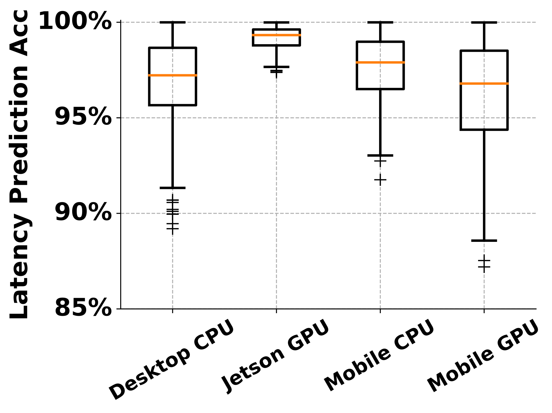
(a) Latency

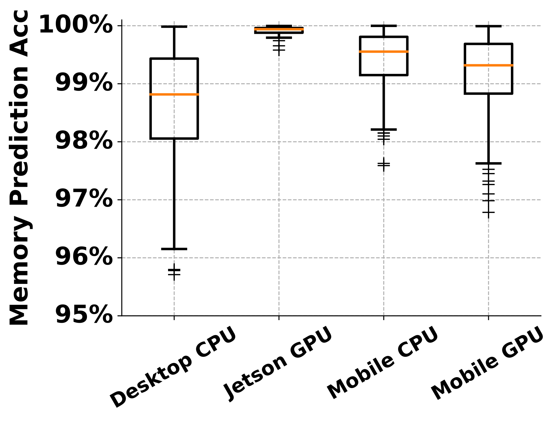
(b) Memory

Figure 8. Performance prediction accuracy of NN-Factory generated models on four edge devices.

Algorithm 1 Lightweight Architecture Search

1:Target edge scenario $e$, task description $task^{e}$, latency requirement ${LAT}^{e}$, memory requirement ${MEM}^{e}$, edge-specific performance evaluator $Evaluator^{e}$.

2:Customized edge model $M$

3:$gate^{opt}\leftarrow NULL$

4:for $limit_{i}$ = 1%; $limit_{i}$ ¡ 1 ; $limit_{i}$ += step do

5:     $enc_{i}\leftarrow Requirement\_Encoding(task^{e},limit_{i})$

6:     $gate_{i}\leftarrow Assembler(enc_{i})$

7:     $lat_{enc},mem_{enc}\leftarrow Evaluator^{e}(gate_{i})$

8:     if $lat_{enc}>{LAT}^{e}$ or $mem_{enc}>{MEM}^{e}$ then

9:         break

10:     end if

11:     $gate^{opt}\leftarrow gate_{i}$

12:end for

13:return the subnet sliced from supernet with $gate^{opt}$

Based on the performance evaluator, we are able to analyze the latency and memory of candidate models. As the more modules activated usually lead to higher accuracy (see Section 5.2), the optimal model for an edge scenario is the one with the highest module activation ratio while satisfying memory and latency requirements. Algorithm 1 shows our lightweight architecture search strategy. We start from the lowest module activation limit $limit_{i}=1\%$, and iteratively raise the limit. For each activation limit, we generate the gate selections using the assembler network, and obtain the latency and memory of related to the gate selections. The last candidate gate selections that meet the edge environment constraints are identified and returned. Finally, we generate the subnet with the result gate selections, which can be directly deployed to the edge without any further processing.

4. Implementation

We implement our method using Python. The training part is based on PyTorch. The models are generated with PyTorch and deployed to edge devices using TensorFlow Lite framework for mobile and PyTorch for Desktop and Jeston

Architecture and Training Details. In the layer gaters of the assembler, we employ distinct batch normalization layers for the selection encoding of different layers, this may influence the quality of the generated model. In order to enhance training stability and improve the quality of the generated model, we augmented the training task set with additional tasks to incorporate more combinations of task properties, which can enhance the model’s understanding of our task encoding. In order to incorporate broader sparsity requirements during training without compromising the model quality, we employ multiple layer gaters to enhance the capacity of the model, drawing on the principles of the Mixture of Experts (MoE), each gater converts the selection encoding into gate selections. Additionally, a gating network is introduced to determine the weighting of outputs from each gater at each layer.

5. Evaluation

We conduct experiments to answer the following questions: (1) Is NN-Factory able to generate edge-specific models? How is the quality of the generated models? (2) How much is the overhead of NN-Factory? (3) How well can the model generation ability of NN-Factory generalize to unseen edge scenarios?

5.1. Experimental Setup

Tasks and Datasets. We evaluated the performance of NN-Factory on two model customization settings.

• Numeric Visual Question Answering (NumVQA). This is a simple setting to analyze the performance of task- and resource-specific model generation. The task is to answer a yes-or-no question (e.g. “Are there two even numbers?”) based on an input image containing four digits. We formulated approximately 60 questions and synthesized images using the MNIST dataset (LeCun et al., 1998). The performance of generated models was measured by the classification accuracy.

• Attributed Object Detection (AttrOD). This is a more practical setting, in which each task is to detect objects with specific attributes in an image and predict the object bounding boxes and categories. We utilized a vision question answering model (Kim et al., 2021) to annotate the object colors in the COCO2017 (Lin et al., 2014) dataset and merged identified colors to form target attributes. We selected 5 attributes (1-white, 2-bronze, 3-charcoal, 4-crimson, 5-chartreuse) from 4 categories and combined them to construct our training tasks. The total number of tasks was approximately 140, and each task has a varying number of samples, ranging from hundreds to tens of thousands. The performance of detection models was measured by mean average precision over Intersection over Union threshold 0.5 (mAP@0.5).

Model Backbones. We considered the common CNN and Transformer backbones in this experiment, including ResNet (He et al., 2016), ViT (Dosovitskiy et al., 2020), for the NumVQA setting and EfficientDet (Tan et al., 2019b) for the AttrOD setting.

Baselines. We compared NN-Factory with two conventional model customization approaches:

1. Retrain - We fixed the model architecture and retrained it with standard supervised learning method for each edge scenario.

2. Prune&Tune - We trained a unified model. Given an edge scenario, we pruned and fine-tuned the pretrained model to match edge requirements with a SOTA pruning method (Fang et al., 2023).

Both of them require training with edge-specific data. We used the same backbones with these baselines and trained them until convergence. We did not include other training-free model generation/scaling methods (Cai et al., 2020b; Han et al., 2021; Fang et al., 2018; Wen et al., 2023) since they don’t support task-oriented customization.

Edge Environments. We considered three edge devices including an Android Smartphone (Xiaomi 12) with Snapdragon® 8 Gen 1 processor and 12GB memory, a Jetson AGX Xavier with 32 GB memory, and a desktop computer with 12th Gen Intel® Core™ i9-12900K $\times$ 24 Processor with 64GB memory. The batch sizes were all set to 1 on the three devices to simulate real workloads. We used different latency budgets to simulate intra-device hardware diversity.

5.2. Model Generation Quality

We conducted an evaluation of the models generated by NN-Factory on NumVQA and AttrOD, followed by a comprehensive analysis of their quality.

Table 2. The quality of generated models on NumVQA.

Generation Request		ResNet		ViT
Task	Act. Limit	Acc	Act. Ratio	Acc	Act. Ratio
Has a number 0	3%	99.7%	3.0%	97.8%	3.0%
Has a number 0	5%	99.8%	3.7%	97.6%	4.0%
Has a number 0	10%	99.9%	3.8%	97.8%	5.1%
Only two number 1	3%	99.3%	3.0%	96.7%	3.0%
Only three number 2	3%	99.4%	3.0%	86.7%	3.0%
Only four number 5	3%	99.1%	3.0%	95.5%	3.0%
Only one number 0	5%	99.8%	3.7%	94.1%	5.0%
Only three number 0	5%	99.4%	3.8%	94.8%	5.0%
Only one number 3	5%	99.8%	3.7%	87.7%	5.0%
Only two odd numbers	3%	99.3%	3.0%	94.3%	3.0%
Only two odd numbers	5%	99.4%	4.0%	94.3%	3.8%

Table 3. The quality of models generated by NN-Factory and baselines for different edge scenarios in the AttrOD setting. The ‘task’ column is the target object followed by the desired attributes (e.g. black, yellow). The ‘Lat’ and ‘Mem’ columns are the relative latency and memory as compared with the requirements ($LAT^{req}$ and $MEM^{req}$).

Edge Scenarios				NN-Factory			Retrain			Prune&Tune
Task	Device	$LAT^{req}$	$MEM^{req}$	$\Delta$Lat	$\Delta$Mem	mAP	$\Delta$Lat	$\Delta$Mem	mAP	$\Delta$Lat	$\Delta$Mem	mAP
Bicycle {3,4}	Desktop	55ms	0.30GB	-0.11	-0.03	0.31	+156.77	+0.38	0.35	-0.33	-0.23	0.34
Person {2}	Desktop	70ms	0.35GB	-4.55	-0.05	0.27	+141.77	+0.33	0.24	-1.05	-0.22	0.22
Car {3}	Desktop	85ms	0.40GB	-2.96	-0.01	0.38	+126.77	+0.28	0.42	-1.77	-0.22	0.41
Motorcycle {1}	Desktop	100ms	0.45GB	-0.05	-0.02	0.45	+111.77	+0.23	0.23	-0.70	-0.21	0.24
Motorcycle {2,3,4}	Desktop	115ms	0.50GB	-2.43	-0.04	0.43	+96.77	+0.18	0.44	-1.42	-0.20	0.45
Bicycle {3,4}	Mobile	350ms	5GB	-47.36	-0.24	0.31	+625.28	+19.97	0.35	-54.4	-0.21	0.34
Motorcycle {5}	Mobile	450ms	7GB	-47.54	-0.07	0.53	+525.28	+17.97	0.19	-86.43	-0.21	0.19
Car {3}	Mobile	550ms	9GB	-25.92	-0.01	0.38	+425.28	+15.97	0.42	-119.46	-0.18	0.41
Person {5}	Jetson	15ms	—	-0.61	—	0.22	+42.98	—	0.15	-0.40	—	0.07
Person {5}	Jetson	20ms	—	-0.81	—	0.22	+37.98	—	0.15	-0.29	—	0.15
Person {5}	Jetson	30ms	—	-0.06	—	0.23	+27.98	—	0.15	-0.08	—	0.16

We first assessed the effectiveness of the modules and assembler in the NumVQA setting. We feed different ¡$task$, $activation\ limit$¿ tuples to the NN-Factory assembler and let it generate models that meet the requirements. The results are presented in Table 2. Overall, NN-Factory demonstrated exceptional accuracy (¿99% with ResNet backbone) across diverse tasks, while also ensuring that the generated models adhered to our specified activation limit. Due to the relatively small task scale, only a lower activation ratio is required.

Next, we evaluated the end-to-end performance of NN-Factory on AttrOD. In Table  3, we employed ResNet50 as the backbone and showcased the quality of the generated models under varying latency and memory requirements on different devices, and compare them with baseline models. Overall, NN-Factory consistently delivers high-quality models that meet the specified criteria in all edge scenarios. Thanks to the performance-aware model architecture search, NN-Factory was able to full utilize the given budgets (either memory or latency). The Retrain baseline failed to meet the latency and memory requirements as it didn’t adjust the model architectures for each scenario.

The accuracy of models generated by NN-Factory is close to the Retrain baseline and outperforms the Prune&Tune baseline, although it doesn’t require edge-specific training. Meanwhile, it managed to achieve significantly higher mAP scores on some tasks (e.g. Motorcycle {1}, Person {5}) that contain less training samples than others. This was because the mixed training of tasks, each with different attribute combinations, enabled the model to achieve a more profound understanding of the tasks and, consequently, make more precise predictions. The accuracy of Prune&Tune models is much lower than NN-Factory and Retrain due to the reduced model size.

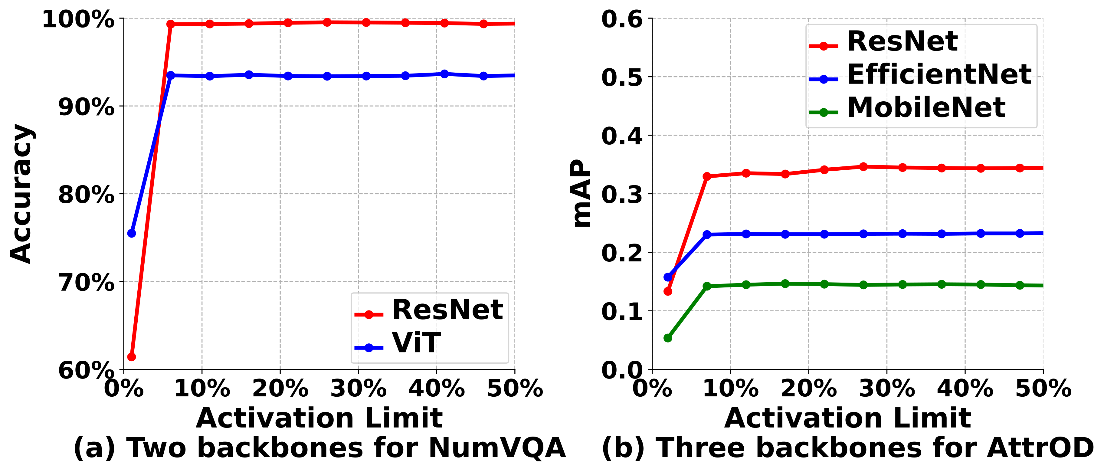
Figure 9. Accuracy of models generated by NN-Factory under different activation limits in NumVQA and AttrOD. The accuracy values are averaged from 10 random tasks.

We also explored the differences in the model quality of NN-Factory with different backbones. The results are displayed in Figure 9. NN-Factory demonstrates consistent behavior across various supernet backbones, signifying its generalizablilty. However, it does exhibit distinct performance differences based on the chosen backbone. For example, the models generated by ViT-based NN-Factory and MobileNet-based NN-Factory exhahited lower accuracy. This was due to the inherent properties of backbone network, e.g. poor sample efficiency of ViT and limited model capability of MobileNet.

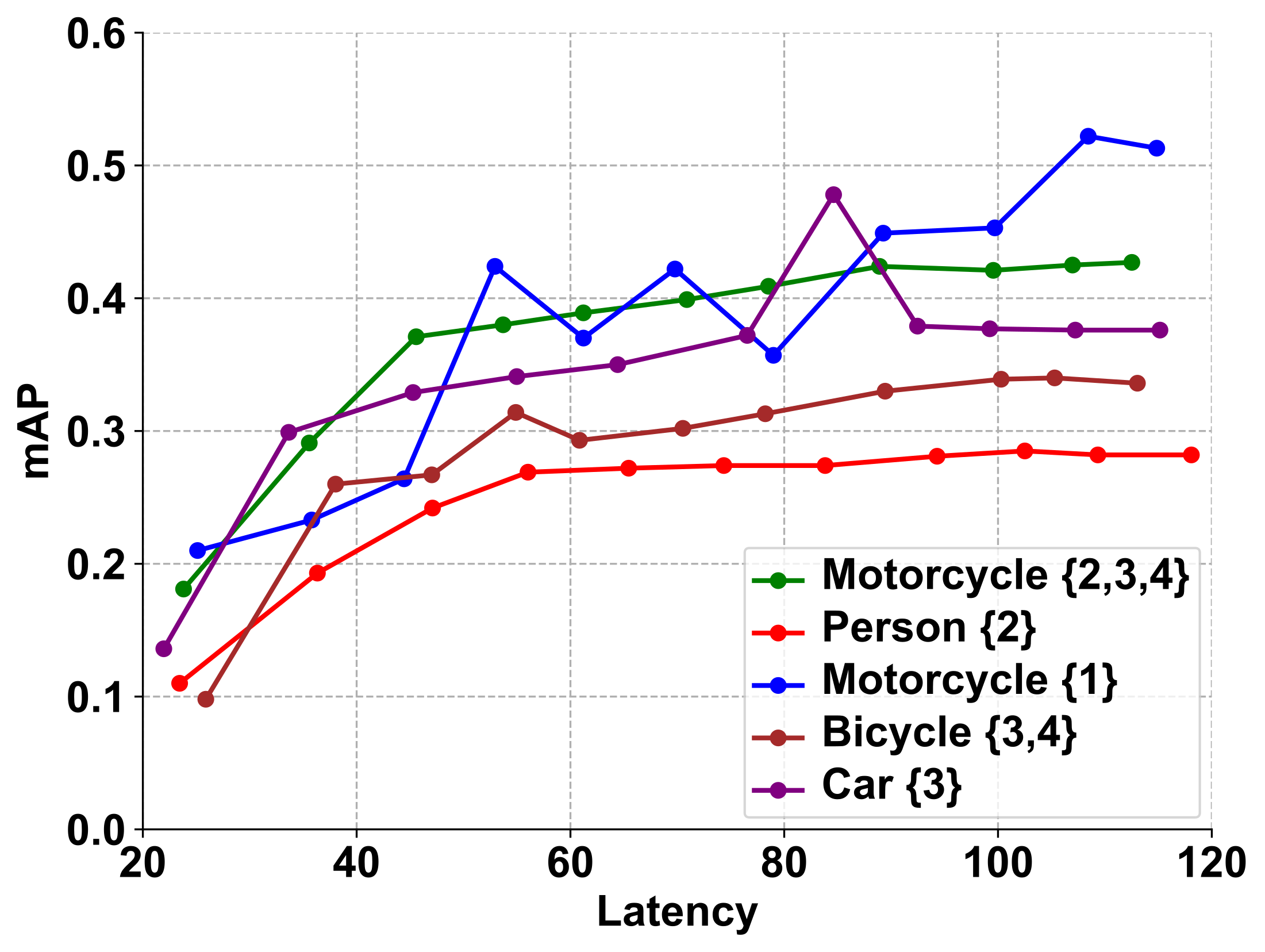
Figure 10. The trade-off between mAP (mean Average Precision) and latency for NN-Factory across different tasks of AttrOD.

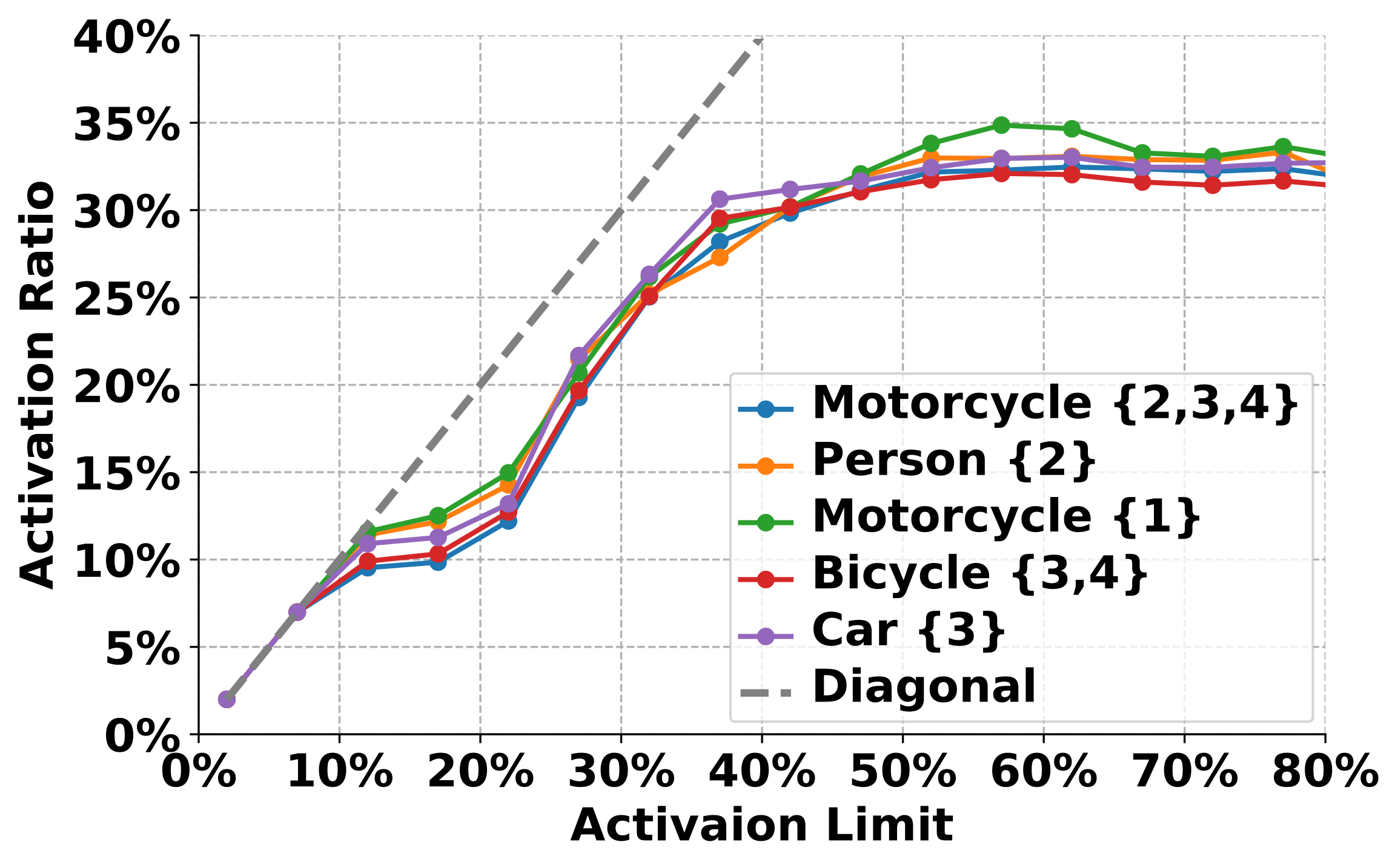
Figure 11. The relation between actual module activation ratio and specified activation limit.

Furthermore, We performed an analysis to evaluate how NN-Factory manages the trade-off between model quality and latency. The results are presented in Figure 10, NN-Factory was capable of generating higher-quality models when given higher latency constraints. Figure 11 illustrates the correlation between the input activation limit during model generation and the activation ratio of the gate selections generated by NN-Factory. With a very low activation limit, generated activation ratio falls short of meeting the requirements. Consequently, it undergoes pruning based on importance, resulting in a pattern that closely aligns with the diagonal on the graph. With the increment of the activation limit, NN-Factory produced activation ratios that could satisfy the criteria. The ratios progressively improved with the increasing activation limits and eventually reached a stable state, because the stabilized ratios were already sufficient to produce the accurate predictions.

5.3. Model Generation Efficiency

Table 4. The preparation time (once for all scenarios) and customization time (once for each edge scenario) of NN-Factory and baselines.

Method	Preparation	Customization
NN-Factory	130 hours	3.6s
Retrain	–	66 hours
Prune&Tune	66 hours	4 hours

We conducted a comparative analysis of preparation and customization costs between NN-Factory and the baselines, and the results are presented in Table 4.

Customization Cost for Each Edge Scenario. The primary goal of NN-Factory is to reduce the model customization time. It took just 3.6 seconds on average for NN-Factory to generate a customized model for an edge scenario, demonstrating remarkable efficiency. This process includes about 12 rounds of searching, each taking 0.2 seconds, and model extraction, which takes 0.8 seconds. In contrast, traditional model customization methods incurred a staggering 4000-fold increase in time because they need to train the model for each edge scenario.

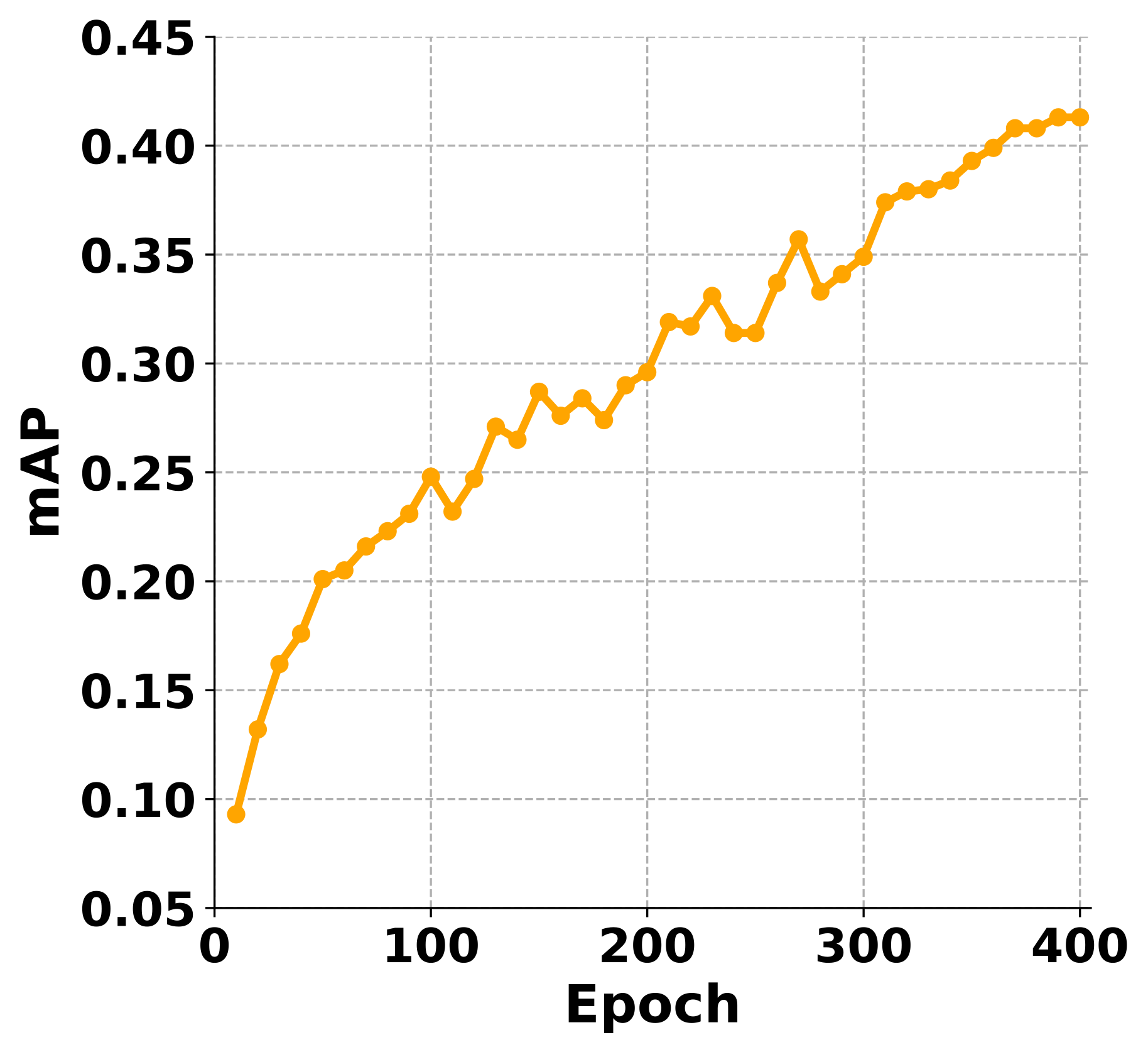
Figure 12. The average accuracy of generated models after training with different #epochs.

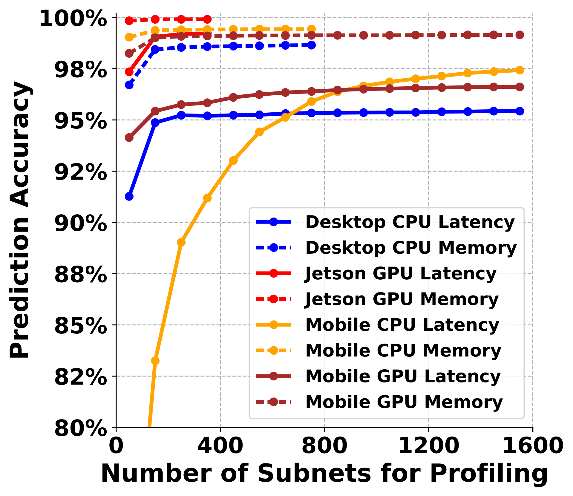
Figure 13. The accuracy of modeling for performance prediction by training with different #subnets.

One-time Preparation Cost. The preparation cost of NN-Factory mainly came from the training of the modular supernet. First, we analyzed the relation between the quality of generated model and number of training epochs. As depicted in Figure  13, NN-Factory requires more training epochs to gradually improve the quality of the generated models. This is associated with our training methodology. NN-Factory undergoes concurrent training on multiple tasks, with each task having access to only a fraction of the training data in each epoch. Consequently, it necessitates more training epochs to produce high-quality models for each individual task. Nonetheless, owing to the substantial inter-dependencies among tasks, their concurrent training has a synergistic effect, ensuring that NN-Factory’s training overhead does not escalate significantly.

The performance predictor used for lightweight architecture search is also built during preparation. Figure 13 shows the performance modeling accuracy achieved with different number of subnets used for profiling and modeling (the supernet backbone is ResNet). As the number of subnets increases, the prediction accuracy shows an upward trend and reaches an asymptotic line. We can see that using 200$\sim$1000 subnets for profiling and training is sufficient to achieve good (higher than 95%) latency and memory prediction accuracy. Collecting the profiling data for one subnet took 70ms (Jetson GPU) to 985ms (Mobile CPU). Meanwhile, the time needed for fitting the performance model is less than few seconds. Therefore, the time to establish the performance prediction model in NN-Factory ranges from approximately 14s to 985s, which is negligible as an offline one-time process.

On-device Serving Cost. The models generated by NN-Factory are normal static models, which do not produce any additional overhead at runtime.

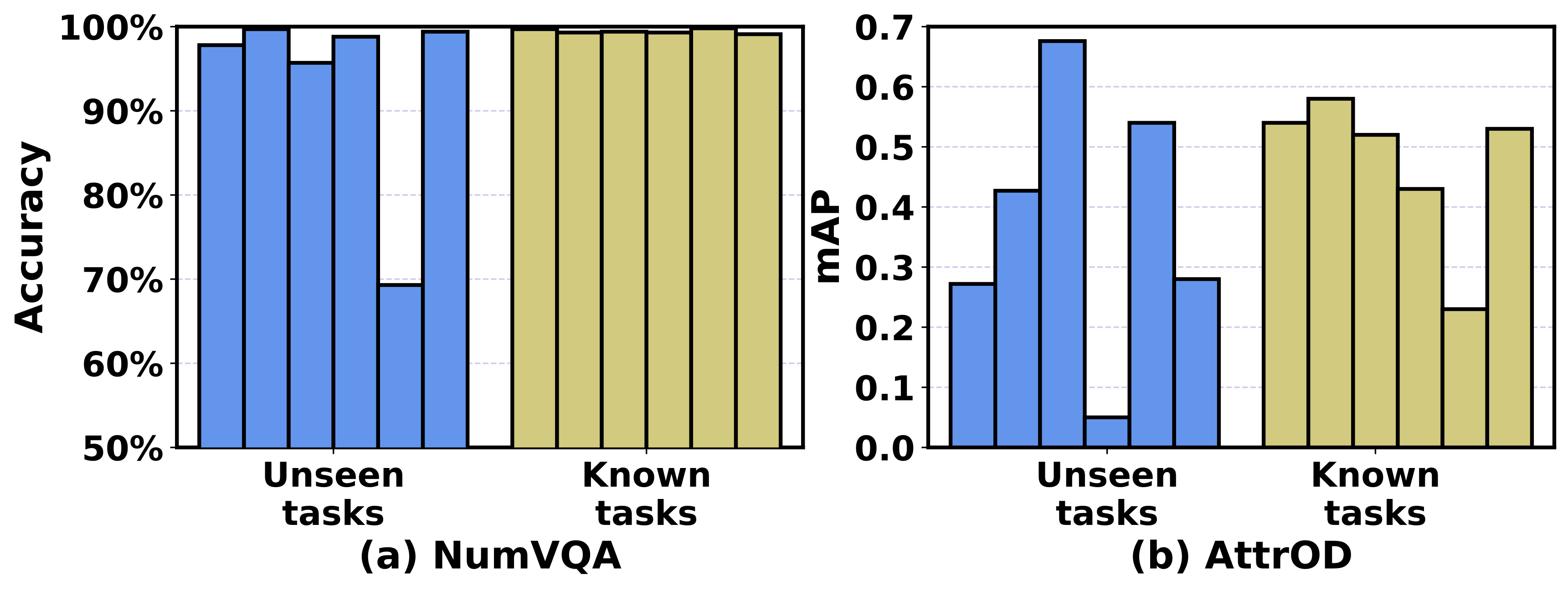
Figure 14. Accuracy or mAP for known & unseen tasks in (a) NumVQA. (b) AttrOD.

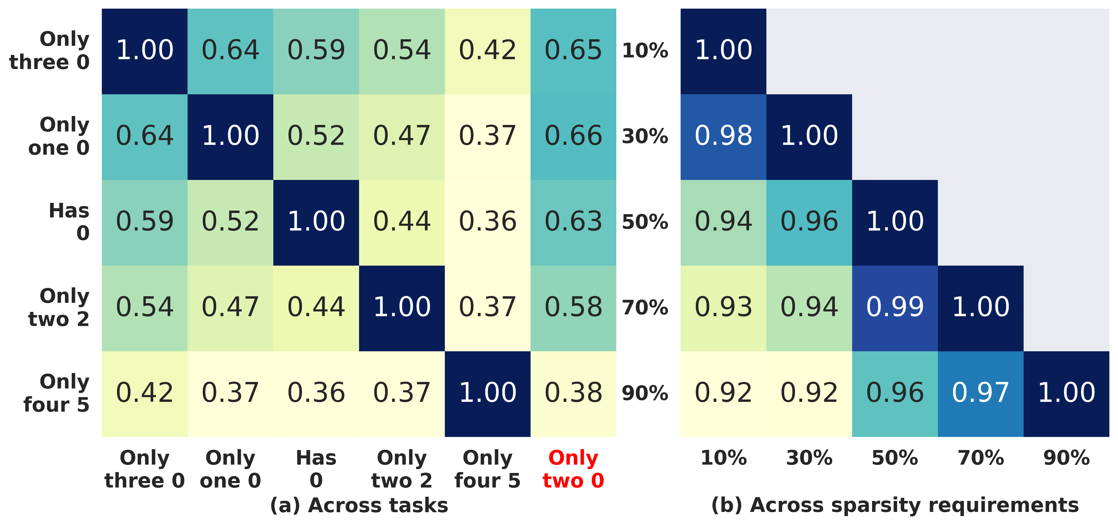
Figure 15. Gate similarity between different tasks (a) and between different activation limits (b) in NumVQA. The task marked in red is an unseen task.

5.4. Generalization to Unseen Tasks

In this section, we evaluate the generalization capability of NN-Factory to unseen tasks. Unseen tasks refer to the tasks that are not part of the training task set, yet they share the same combinatorial property space as the training tasks.

Figure 14 illustrates the accuracy of randomly selected unseen tasks in NumVQA and AttrOD. Although the accuracy for unseen tasks may exhibit a slight reduction as compared to that of known tasks and few unseen tasks may even yield a much lower accuracy, the majority of tasks demonstrate excellent accuracy, meaning that the modules in NN-Factory can be effectively assembled to handle new tasks without training data. This result highlights the robust generalization capabilities of NN-Factory, as it can grasp the meanings of the properties comprising a task and comprehend the operations involved in their combinations.

We further analyzed the generalization capabilities of NN-Factory based on the similarity between the gate selections for different tasks. The result is presented in Figure 15. The gate selections exhibit higher similarity when tasks are more alike (e.g. ‘Only one 0’ and ‘Only three 0’). Additionally, within a fixed task, increased proximity in the given activation limits leads to greater similarity in gate selections. This demonstrates the ability of NN-Factory to understand both the specified task and activation limit requirements, and map them to corresponding modules. This serves as the underpinning for its generalization abilities.

With this ability, NN-Factory can identify the most relevant modules for an unseen task and assemble a model with them. For example, the activated modules for the unseen ‘only two 0’ task are similar with the modules of ‘only three 0’ and ‘only one 0’ in Figure 15. This leads to a high accuracy on the unseen task. Therefore, the generalization capability of NN-Factory is positively correlated with the number of tasks for training, which can lead to more useful modules and a more powerful assembler.

6. Discussion

Here we highlight some issues that warrant further discussion.

Applicability to other types of tasks. Currently, NN-Factory only support customizing models for tasks that are in a combinatorial space, which may limit its applicability to more generic usage scenarios. To enable more flexible task spaces, we need to use a more powerful generative model as the assembler, which takes free-form task definition (e.g. natural language task description) as the input, and operates on a larger set of neural modules. Meanwhile, a large dataset containing the mappings between different tasks and corresponding input/output pairs is required to train the assembler and modules. This is feasible according to the recent advances of pretrained large models (e.g. ImageBind, ChatGPT, etc.), but training such a general-purpose model generator is very time-consuming and resource-intensive, which is impractical for most researchers. We leave the development of such general-purpose NN-Factory for future work.

Preparation cost of NN-Factory. The remarkable rapid model customization ability of NN-Factory comes at the cost of longer offline preparation time. Specifically, training the modular supernet and the module assembler takes much longer time than training a normal static model. This is because that NN-Factory needs to not only learn how to solve each individual task, but also how to decouple the modules and reassemble them to solve new tasks. Considering the reduced marginal cost for supporting diverse edge scenarios, the one-time preparation cost is less significant. Such benefits of marginal cost reduction are more valuable if NN-Factory supports more flexible task spaces.

7. Conclusion

This paper proposes a novel approach for rapid customization of deep learning models for diverse edge scenarios. With a holistic design with a modular supernet, a module assembler, and a lightweight architecture searcher, we are able to achieve rapid model customization for deverse edge tasks and resource constraints. Experiments have demonstrated excellent model generation quality and speed of our approach. We believe our work has enabled a new and important generative model customization experience.

References

- (1)
- Andreas et al. (2016) Jacob Andreas, Marcus Rohrbach, Trevor Darrell, and Dan Klein. 2016. Neural module networks. In Proceedings of the IEEE conference on computer vision and pattern recognition. 39–48.
- Bolukbasi et al. (2017) Tolga Bolukbasi, Joseph Wang, Ofer Dekel, and Venkatesh Saligrama. 2017. Adaptive Neural Networks for Efficient Inference. In Proceedings of the 34th International Conference on Machine Learning - Volume 70 (ICML’17). JMLR.org, 527–536.
- Cai et al. (2020a) Han Cai, Chuang Gan, Tianzhe Wang, Zhekai Zhang, and Song Han. 2020a. Once for All: Train One Network and Specialize it for Efficient Deployment. In International Conference on Learning Representations. https://arxiv.org/pdf/1908.09791.pdf
- Cai et al. (2020b) Han Cai, Chuang Gan, Tianzhe Wang, Zhekai Zhang, and Song Han. 2020b. Once-for-All: Train One Network and Specialize it for Efficient Deployment. In 8th International Conference on Learning Representations, ICLR 2020.
- Cai et al. (2019) Han Cai, Ligeng Zhu, and Song Han. 2019. ProxylessNAS: Direct Neural Architecture Search on Target Task and Hardware. In International Conference on Learning Representations. https://arxiv.org/pdf/1812.00332.pdf
- Chen et al. (2017) Yimin Chen, Jingchao Sun, Xiaocong Jin, Tao Li, Rui Zhang, and Yanchao Zhang. 2017. Your face your heart: Secure mobile face authentication with photoplethysmograms. In IEEE INFOCOM 2017 - IEEE Conference on Computer Communications. 1–9. https://doi.org/10.1109/INFOCOM.2017.8057220
- Chowdhery et al. (2022) Aakanksha Chowdhery, Sharan Narang, Jacob Devlin, Maarten Bosma, Gaurav Mishra, Adam Roberts, Paul Barham, Hyung Won Chung, Charles Sutton, Sebastian Gehrmann, et al. 2022. Palm: Scaling language modeling with pathways. arXiv preprint arXiv:2204.02311 (2022).
- Creswell et al. (2018) Antonia Creswell, Tom White, Vincent Dumoulin, Kai Arulkumaran, Biswa Sengupta, and Anil A Bharath. 2018. Generative adversarial networks: An overview. IEEE signal processing magazine 35, 1 (2018), 53–65.
- Croitoru et al. (2023) Florinel-Alin Croitoru, Vlad Hondru, Radu Tudor Ionescu, and Mubarak Shah. 2023. Diffusion models in vision: A survey. IEEE Transactions on Pattern Analysis and Machine Intelligence (2023).
- Dai et al. (2021) Damai Dai, Li Dong, Yaru Hao, Zhifang Sui, Baobao Chang, and Furu Wei. 2021. Knowledge neurons in pretrained transformers. arXiv preprint arXiv:2104.08696 (2021).
- Dosovitskiy et al. (2020) Alexey Dosovitskiy, Lucas Beyer, Alexander Kolesnikov, Dirk Weissenborn, Xiaohua Zhai, Thomas Unterthiner, Mostafa Dehghani, Matthias Minderer, Georg Heigold, Sylvain Gelly, Jakob Uszkoreit, and Neil Houlsby. 2020. An Image is Worth 16x16 Words: Transformers for Image Recognition at Scale. arXiv preprint arXiv:2010.11929 (2020).
- Fang et al. (2020) Biyi Fang, Xiao Zeng, Faen Zhang, Hui Xu, and Mi Zhang. 2020. FlexDNN: Input-Adaptive On-Device Deep Learning for Efficient Mobile Vision. In 2020 IEEE/ACM Symposium on Edge Computing (SEC). 84–95. https://doi.org/10.1109/SEC50012.2020.00014
- Fang et al. (2018) Biyi Fang, Xiao Zeng, and Mi Zhang. 2018. NestDNN: Resource-Aware Multi-Tenant On-Device Deep Learning for Continuous Mobile Vision. Proceedings of the 24th Annual International Conference on Mobile Computing and Networking (2018).
- Fang et al. (2023) Gongfan Fang, Xinyin Ma, Mingli Song, Michael Bi Mi, and Xinchao Wang. 2023. Depgraph: Towards any structural pruning. In Proceedings of the IEEE/CVF Conference on Computer Vision and Pattern Recognition. 16091–16101.
- Guo et al. (2021) Peizhen Guo, Bo Hu, and Wenjun Hu. 2021. Mistify: Automating DNN Model Porting for On-Device Inference at the Edge. In 18th USENIX Symposium on Networked Systems Design and Implementation (NSDI 21). USENIX Association, 705–719. https://www.usenix.org/conference/nsdi21/presentation/guo
- Guo et al. (2020) Zichao Guo, Xiangyu Zhang, Haoyuan Mu, Wen Heng, Zechun Liu, Yichen Wei, and Jian Sun. 2020. Single Path One-Shot Neural Architecture Search with Uniform Sampling. In Computer Vision – ECCV 2020, Andrea Vedaldi, Horst Bischof, Thomas Brox, and Jan-Michael Frahm (Eds.). Springer International Publishing, Cham, 544–560.
- Han et al. (2021) Rui Han, Qinglong Zhang, Chi Harold Liu, Guoren Wang, Jian Tang, and Lydia Y. Chen. 2021. LegoDNN: Block-Grained Scaling of Deep Neural Networks for Mobile Vision. In Proceedings of the 27th Annual International Conference on Mobile Computing and Networking (MobiCom ’21). Association for Computing Machinery, New York, NY, USA, 406–419. https://doi.org/10.1145/3447993.3483249
- Han et al. (2016) Song Han, Huizi Mao, and William J. Dally. 2016. Deep Compression: Compressing Deep Neural Network with Pruning, Trained Quantization and Huffman Coding. arXiv: Computer Vision and Pattern Recognition (2016).
- Han et al. (2022) Yizeng Han, Gao Huang, Shiji Song, Le Yang, Honghui Wang, and Yulin Wang. 2022. Dynamic Neural Networks: A Survey. IEEE Transactions on Pattern Analysis and Machine Intelligence 44, 11 (2022), 7436–7456. https://doi.org/10.1109/TPAMI.2021.3117837
- He et al. (2016) Kaiming He, Xiangyu Zhang, Shaoqing Ren, and Jian Sun. 2016. Deep Residual Learning for Image Recognition. In 2016 IEEE Conference on Computer Vision and Pattern Recognition (CVPR). 770–778. https://doi.org/10.1109/CVPR.2016.90
- He et al. (2021) Yuze He, Li Ma, Zhehao Jiang, Yi Tang, and Guoliang Xing. 2021. VI-Eye: Semantic-Based 3D Point Cloud Registration for Infrastructure-Assisted Autonomous Driving. In Proceedings of the 27th Annual International Conference on Mobile Computing and Networking (MobiCom ’21). Association for Computing Machinery, New York, NY, USA, 573–586. https://doi.org/10.1145/3447993.3483276
- Huang and Chu (2021) Sian-Yao Huang and Wei-Ta Chu. 2021. Searching by Generating: Flexible and Efficient One-Shot NAS with Architecture Generator. In Proceedings of IEEE Conference on Computer Vision and Pattern Recognition.
- Jacobs et al. (1991) Robert A Jacobs, Michael I Jordan, Steven J Nowlan, and Geoffrey E Hinton. 1991. Adaptive mixtures of local experts. Neural computation 3, 1 (1991), 79–87.
- Jeon et al. (2023) Seunghyeok Jeon, Yonghun Choi, Yeonwoo Cho, and Hojung Cha. 2023. HarvNet: Resource-Optimized Operation of Multi-Exit Deep Neural Networks on Energy Harvesting Devices. In Proceedings of the 21st Annual International Conference on Mobile Systems, Applications and Services (MobiSys ’23). Association for Computing Machinery, New York, NY, USA, 42–55. https://doi.org/10.1145/3581791.3596845
- Jiang et al. (2021) Shiqi Jiang, Zhiqi Lin, Yuanchun Li, Yuanchao Shu, and Yunxin Liu. 2021. Flexible high-resolution object detection on edge devices with tunable latency. In Proceedings of the 27th Annual International Conference on Mobile Computing and Networking. 559–572.
- Kaiser and Bengio (2018) Łukasz Kaiser and Samy Bengio. 2018. Discrete autoencoders for sequence models. arXiv preprint arXiv:1801.09797 (2018).
- Kaiser et al. (2018) Lukasz Kaiser, Samy Bengio, Aurko Roy, Ashish Vaswani, Niki Parmar, Jakob Uszkoreit, and Noam Shazeer. 2018. Fast decoding in sequence models using discrete latent variables. In International Conference on Machine Learning. PMLR, 2390–2399.
- Kaplan et al. (2020) Jared Kaplan, Sam McCandlish, Tom Henighan, Tom B Brown, Benjamin Chess, Rewon Child, Scott Gray, Alec Radford, Jeffrey Wu, and Dario Amodei. 2020. Scaling laws for neural language models. arXiv preprint arXiv:2001.08361 (2020).
- Kim et al. (2021) Wonjae Kim, Bokyung Son, and Ildoo Kim. 2021. Vilt: Vision-and-language transformer without convolution or region supervision. In International Conference on Machine Learning. PMLR, 5583–5594.
- Kong et al. (2023) Rui Kong, Yuanchun Li, Yizhen Yuan, and Linghe Kong. 2023. ConvReLU++: Reference-Based Lossless Acceleration of Conv-ReLU Operations on Mobile CPU. In Proceedings of the 21st Annual International Conference on Mobile Systems, Applications and Services (MobiSys ’23). Association for Computing Machinery, New York, NY, USA, 503–515. https://doi.org/10.1145/3581791.3596831
- Laskaridis et al. (2021) Stefanos Laskaridis, Alexandros Kouris, and Nicholas D. Lane. 2021. Adaptive Inference through Early-Exit Networks: Design, Challenges and Directions. In Proceedings of the 5th International Workshop on Embedded and Mobile Deep Learning (EMDL’21). Association for Computing Machinery, New York, NY, USA, 1–6. https://doi.org/10.1145/3469116.3470012
- Laskaridis et al. (2020) Stefanos Laskaridis, Stylianos I. Venieris, Hyeji Kim, and Nicholas D. Lane. 2020. HAPI: Hardware-Aware Progressive Inference. In 2020 IEEE/ACM International Conference On Computer Aided Design (ICCAD). 1–9.
- LeCun et al. (1998) Yann LeCun, Léon Bottou, Yoshua Bengio, and Patrick Haffner. 1998. Gradient-based learning applied to document recognition. Proc. IEEE 86, 11 (1998), 2278–2324.
- Li et al. (2020) Changlin Li, Jiefeng Peng, Liuchun Yuan, Guangrun Wang, Xiaodan Liang, Liang Lin, and Xiaojun Chang. 2020. Block-Wisely Supervised Neural Architecture Search With Knowledge Distillation. In 2020 IEEE/CVF Conference on Computer Vision and Pattern Recognition (CVPR). 1986–1995. https://doi.org/10.1109/CVPR42600.2020.00206
- Lin et al. (2014) Tsung-Yi Lin, Michael Maire, Serge J. Belongie, Lubomir D. Bourdev, Ross B. Girshick, James Hays, Pietro Perona, Deva Ramanan, Piotr Dollár, and C. Lawrence Zitnick. 2014. Microsoft COCO: Common Objects in Context. CoRR abs/1405.0312 (2014). arXiv:1405.0312 http://arxiv.org/abs/1405.0312
- Liu et al. (2020) Bingyan Liu, Yuanchun Li, Yunxin Liu, Yao Guo, and Xiangqun Chen. 2020. Pmc: A privacy-preserving deep learning model customization framework for edge computing. Proceedings of the ACM on Interactive, Mobile, Wearable and Ubiquitous Technologies 4, 4 (2020), 1–25.
- Liu et al. (2021) Chia-Hsiang Liu, Yu-Shin Han, Yuan-Yao Sung, Yi Lee, Hung-Yueh Chiang, and Kai-Chiang Wu. 2021. FOX-NAS: Fast, On-device and Explainable Neural Architecture Search. CoRR abs/2108.08189 (2021). arXiv:2108.08189 https://arxiv.org/abs/2108.08189
- Liu et al. (2018) Hanxiao Liu, Karen Simonyan, and Yiming Yang. 2018. DARTS: Differentiable Architecture Search. CoRR abs/1806.09055 (2018). arXiv:1806.09055 http://arxiv.org/abs/1806.09055
- Liu et al. (2017) Zhuang Liu, Jianguo Li, Zhiqiang Shen, Gao Huang, Shoumeng Yan, and Changshui Zhang. 2017. Learning Efficient Convolutional Networks through Network Slimming. In 2017 IEEE International Conference on Computer Vision (ICCV). 2755–2763. https://doi.org/10.1109/ICCV.2017.298
- OpenAI (2022) OpenAI. 2022. ChatGPT. [Online]. Available at: https://openai.com/blog/chatgpt/.
- Parisotto et al. (2016) Emilio Parisotto, Abdel-rahman Mohamed, Rishabh Singh, Lihong Li, Dengyong Zhou, and Pushmeet Kohli. 2016. Neuro-symbolic program synthesis. arXiv preprint arXiv:1611.01855 (2016).
- Park et al. (2018) Jinhwan Park, Yoonho Boo, Iksoo Choi, Sungho Shin, and Wonyong Sung. 2018. Fully Neural Network Based Speech Recognition on Mobile and Embedded Devices. In NeurIPS.
- Real et al. (2019) Esteban Real, Alok Aggarwal, Yanping Huang, and Quoc V. Le. 2019. Regularized Evolution for Image Classifier Architecture Search. In Proceedings of the Thirty-Third AAAI Conference on Artificial Intelligence and Thirty-First Innovative Applications of Artificial Intelligence Conference and Ninth AAAI Symposium on Educational Advances in Artificial Intelligence (AAAI’19/IAAI’19/EAAI’19). AAAI Press, Article 587, 10 pages. https://doi.org/10.1609/aaai.v33i01.33014780
- Sandler et al. (2018) Mark Sandler, Andrew Howard, Menglong Zhu, Andrey Zhmoginov, and Liang-Chieh Chen. 2018. MobileNetV2: Inverted Residuals and Linear Bottlenecks. In 2018 IEEE/CVF Conference on Computer Vision and Pattern Recognition. 4510–4520. https://doi.org/10.1109/CVPR.2018.00474
- Tan et al. (2019a) Mingxing Tan, Bo Chen, Ruoming Pang, Vijay Vasudevan, Mark Sandler, Andrew Howard, and Quoc V. Le. 2019a. MnasNet: Platform-Aware Neural Architecture Search for Mobile. In 2019 IEEE/CVF Conference on Computer Vision and Pattern Recognition (CVPR). 2815–2823. https://doi.org/10.1109/CVPR.2019.00293
- Tan and Le (2021) Mingxing Tan and Quoc Le. 2021. EfficientNetV2: Smaller Models and Faster Training. In Proceedings of the 38th International Conference on Machine Learning (Proceedings of Machine Learning Research), Marina Meila and Tong Zhang (Eds.), Vol. 139. PMLR, 10096–10106. https://proceedings.mlr.press/v139/tan21a.html
- Tan and Le (2019) Mingxing Tan and Quoc V Le. 2019. EfficientNet: Rethinking Model Scaling for Convolutional Neural Networks. ICML (2019).
- Tan et al. (2019b) Mingxing Tan, Ruoming Pang, and Quoc V. Le. 2019b. EfficientDet: Scalable and Efficient Object Detection. CoRR abs/1911.09070 (2019). arXiv:1911.09070 http://arxiv.org/abs/1911.09070
- Vaswani et al. (2017) Ashish Vaswani, Noam Shazeer, Niki Parmar, Jakob Uszkoreit, Llion Jones, Aidan N. Gomez, Łukasz Kaiser, and Illia Polosukhin. 2017. Attention is All You Need. In Proceedings of the 31st International Conference on Neural Information Processing Systems (NIPS’17). Curran Associates Inc., Red Hook, NY, USA, 6000–6010.
- Wang et al. (2019) Kuan Wang, Zhijian Liu, Yujun Lin, Ji Lin, and Song Han. 2019. HAQ: Hardware-Aware Automated Quantization With Mixed Precision. In IEEE Conference on Computer Vision and Pattern Recognition (CVPR).
- Wang et al. (2020) Quan Wang, Ignacio Lopez Moreno, Mert Saglam, Kevin Wilson, Alan Chiao, Renjie Liu, Yanzhang He, Wei Li, Jason Pelecanos, Marily Nika, et al. 2020. VoiceFilter-Lite: Streaming targeted voice separation for on-device speech recognition. arXiv preprint arXiv:2009.04323 (2020).
- Wang et al. (2018) Xin Wang, Fisher Yu, Zi-Yi Dou, Trevor Darrell, and Joseph E. Gonzalez. 2018. SkipNet: Learning Dynamic Routing in Convolutional Networks. In The European Conference on Computer Vision (ECCV).
- Wen et al. (2023) Hao Wen, Yuanchun Li, Zunshuai Zhang, Shiqi Jiang, Xiaozhou Ye, Ye Ouyang, Ya-Qin Zhang, and Yunxin Liu. 2023. AdaptiveNet: Post-deployment Neural Architecture Adaptation for Diverse Edge Environments. (2023).
- Wu et al. (2019) Bichen Wu, Xiaoliang Dai, Peizhao Zhang, Yanghan Wang, Fei Sun, Yiming Wu, Yuandong Tian, Peter Vajda, Yangqing Jia, and Kurt Keutzer. 2019. FBNet: Hardware-Aware Efficient ConvNet Design via Differentiable Neural Architecture Search. In 2019 IEEE/CVF Conference on Computer Vision and Pattern Recognition (CVPR). 10726–10734. https://doi.org/10.1109/CVPR.2019.01099
- Wu et al. (2018) Zuxuan Wu, Tushar Nagarajan, Abhishek Kumar, Steven Rennie, Larry S Davis, Kristen Grauman, and Rogerio Feris. 2018. BlockDrop: Dynamic Inference Paths in Residual Networks. In CVPR.
- Yang et al. (2018) Tien-Ju Yang, Andrew Howard, Bo Chen, Xiao Zhang, Alec Go, Mark Sandler, Vivienne Sze, and Hartwig Adam. 2018. NetAdapt: Platform-Aware Neural Network Adaptation for Mobile Applications. In The European Conference on Computer Vision (ECCV).
- Yu and Huang (2019) Jiahui Yu and Thomas S. Huang. 2019. Universally Slimmable Networks and Improved Training Techniques. CoRR abs/1903.05134 (2019). arXiv:1903.05134 http://arxiv.org/abs/1903.05134
- Yu et al. (2018) Jiahui Yu, Linjie Yang, Ning Xu, Jianchao Yang, and Thomas S. Huang. 2018. Slimmable Neural Networks. CoRR abs/1812.08928 (2018). arXiv:1812.08928 http://arxiv.org/abs/1812.08928
- Zhang et al. (2021c) Huanhuan Zhang, Anfu Zhou, Yuhan Hu, Chaoyue Li, Guangping Wang, Xinyu Zhang, Huadong Ma, Leilei Wu, Aiyun Chen, and Changhui Wu. 2021c. Loki: Improving Long Tail Performance of Learning-Based Real-Time Video Adaptation by Fusing Rule-Based Models. In Proceedings of the 27th Annual International Conference on Mobile Computing and Networking (MobiCom ’21). Association for Computing Machinery, New York, NY, USA, 775–788. https://doi.org/10.1145/3447993.3483259
- Zhang et al. (2021b) Xumiao Zhang, Anlan Zhang, Jiachen Sun, Xiao Zhu, Y. Ethan Guo, Feng Qian, and Z. Morley Mao. 2021b. EMP: Edge-Assisted Multi-Vehicle Perception. In Proceedings of the 27th Annual International Conference on Mobile Computing and Networking (MobiCom ’21). Association for Computing Machinery, New York, NY, USA, 545–558. https://doi.org/10.1145/3447993.3483242
- Zhang et al. (2020) Ziqi Zhang, Yuanchun Li, Yao Guo, Xiangqun Chen, and Yunxin Liu. 2020. Dynamic slicing for deep neural networks. In Proceedings of the 28th ACM Joint Meeting on European Software Engineering Conference and Symposium on the Foundations of Software Engineering. 838–850.
- Zhang et al. (2023) Ziqi Zhang, Yuanchun Li, Bingyan Liu, Yifeng Cai, Ding Li, Yao Guo, and Xiangqun Chen. 2023. FedSlice: Protecting Federated Learning Models from Malicious Participants with Model Slicing. In 2023 IEEE/ACM 45th International Conference on Software Engineering (ICSE). IEEE, 460–472.
- Zhang et al. (2022) Ziqi Zhang, Yuanchun Li, Jindong Wang, Bingyan Liu, Ding Li, Yao Guo, Xiangqun Chen, and Yunxin Liu. 2022. ReMoS: reducing defect inheritance in transfer learning via relevant model slicing. In Proceedings of the 44th International Conference on Software Engineering. 1856–1868.
- Zhang et al. (2021a) Zhengyan Zhang, Yankai Lin, Zhiyuan Liu, Peng Li, Maosong Sun, and Jie Zhou. 2021a. Moefication: Transformer feed-forward layers are mixtures of experts. arXiv preprint arXiv:2110.01786 (2021).
- Zhu et al. (2020) Feng Zhu, Ruihao Gong, Fengwei Yu, Xianglong Liu, Yanfei Wang, Zhelong Li, Xiuqi Yang, and Junjie Yan. 2020. Towards Unified INT8 Training for Convolutional Neural Network. In 2020 IEEE/CVF Conference on Computer Vision and Pattern Recognition (CVPR). 1966–1976. https://doi.org/10.1109/CVPR42600.2020.00204
- Zoph and Le (2016) Barret Zoph and Quoc V. Le. 2016. Neural Architecture Search with Reinforcement Learning. CoRR abs/1611.01578 (2016). arXiv:1611.01578 http://arxiv.org/abs/1611.01578