The projected dynamic linear model for time series on the sphere

Abstract

Time series on the unit $n$-sphere arise in directional statistics, compositional data analysis, and many scientific fields. There are few models for such data, and the ones that exist suffer from several limitations: they are often challenging to fit computationally, many of them apply only to the circular case of $n=2$, and they are usually based on families of distributions that are not flexible enough to capture the complexities observed in real data. Furthermore, there is little work on Bayesian methods for spherical time series. To address these shortcomings, we propose a state space model based on the projected normal distribution that can be applied to spherical time series of arbitrary dimension. We describe how to perform fully Bayesian offline inference for this model using a simple and efficient Gibbs sampling algorithm, and we develop a Rao-Blackwellized particle filter to perform online inference for streaming data. In an analysis of wind direction time series, we show that the proposed model outperforms competitors in terms of point, interval, and density forecasting.

1 Introduction

Time series that take values on the unit $n$-sphere $S^{n-1}=\{\mathbf{u}\in\mathbb{R}^{n}:||\mathbf{u}||_{2}=1\}$ arise in many fields. In directional statistics, we collect measurements on the orientation or direction-of-travel of an object, and these data can be recorded as points on $S^{1}$ or $S^{2}$ (Pewsey and García-Portugués, 2021). Weather stations across the globe, for example, collect high frequency time series on the direction-of-arrival of the wind, and modeling this variable is important for monitoring the spread of wildfires or air pollution (García-Portugués et al., 2013; García-Portugués et al., 2014). In compositional data analysis, we collect measurements on the standard simplex $C^{n-1}=\{\mathbf{p}\in\mathbb{R}^{n}:\sum_{i=1}^{n}p_{i}=1,\,p_{i}\geq 0\}$, and these data can represent proportions of a total such as the market shares of firms in an industry or the fraction of total electricity produced by different energy sources. The simplex-structure of these data pose many challenges, but one promising approach advocated by Scealy and Welsh (2011) and others is to apply a square root transformation to compositional data, thus turning it into unit vector data that can be analyzed using spherical methods.

Because $S^{n-1}\subseteq\mathbb{R}^{n}$ is a non-Euclidean manifold, naively applying familiar linear, Gaussian methods to spherical time series can generate distorted and misleading results. To see this, consider the simplest instance of spherical time series: the circular case with $n=2$. In this case, $S^{1}$ is the unit circle in the plane, so a unit vector $\mathbf{u}_{t}\in S^{1}$ can alternatively be represented as an angle $a_{t}\in[0,\,2\pi)$, and the correspondence between the two is given by $\mathbf{u}_{t}=[\cos a_{t}\,\sin a_{t}]^{\scriptscriptstyle\mathsf{T}}$ and $a_{t}=\text{atan2}(\mathbf{u}_{t})\text{ mod }2\pi$. Figure 1 displays a classic time series from Fisher (1993) of the hourly direction-of-arrival of the wind at Black Mountain in Australia. The wind in this example is generally blowing from a south easterly direction, and occasionally it passes counterclockwise across the $0/2\pi$ break on the unit circle. On a plot this phenomenon presents as abrupt spikes in the time series of angles. If we naively apply a standard method like a local-level dynamic linear model to these data, we get a (smoothed) trend estimate like the blue in Figure 1, which overfits to the spikes because the linear, Gaussian model does not understand the “wrapped” structure of the circle. If instead we apply a model that does understand this structure, such as the projected dynamic linear model that we introduce in Section 2, we get a more reasonable trend estimate in red. This illustrates the nature of the problem in the simplest case of $n=2$, and matters only get worse in higher dimensions.

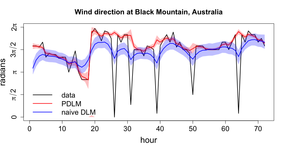
Figure 1: Trend estimates (posterior median and 50% credible band) from a non-circular model (27, 28) in blue and our circular model (1, 2, 3) in red.

1.1 Previous work

	coherent	general	predictive	sequential	exact	parameters	software
naive (V)AR	No	Yes	Yes	Yes	Yes	Yes	Yes
naive DLM	No	Yes	Yes	partial	Yes	partial	Yes
WAR	Yes	No	Yes	No	Yes	Yes	No
LAR	Yes	No	Yes	No	Yes	Yes	No
WN-SSM	Yes	No	Yes	Yes	No	No	Yes
vMF-SSM	Yes	Yes	Yes	Yes	No	No	Yes
SAR	Yes	Yes	No	No	Yes	Yes	No
PDLM	Yes	Yes	Yes	partial	Yes	partial	Yes

Table 1: The proposed PDLM fully or partially satisfies all of the desired properties of a time series model for spherical data.

Ideally, a model for spherical time series would possess the following properties:

• data coherence: as the example in Figure 1 demonstrates, naive linear, Gaussian methods generate distorted results. It is necessary to apply methods that take into account the special structure of the sphere by, for instance, making use of probability distributions supported on the sphere;

• generalize to the hyperspherical case: circular data with $n=2$ is an important special case, but we want a modeling framework that generalizes easily to the spherical ($n=3$) and hyperspherical ($n>3$) cases as well;

• generate full predictive distributions: instead of just generating point forecasts, we want an approach that can generate flexible predictive distributions that acknowledge as many sources of uncertainty as possible. This is most commonly achieved by taking a Bayesian approach to inference and using the posterior predictive distribution;

• sequential inference for streaming data: in the time series setting, observations are often streaming by in real-time and potentially at high frequency, and we wish to recursively update our inferences and predictions in an efficient way to adapt to incoming data;

• exact inference: we would like our statistical computations to be “exact” in the sense that estimates, predictions, or posterior distributions can be approximated arbitrarily well in the limit of some algorithm setting that the user has perfect control over, such as the number of samples in a Monte Carlo algorithm;

• jointly estimate static and dynamic unobservables: in the context of state space models, there are usually static parameters that also need to be estimated along with the dynamic latent states. This is challenging to do in general, and even when it can be done, it is often difficult to do while also performing sequential inference;

• provide software: estimation for circular and spherical time series models is often numerically delicate, and the less the user has to code themselves, the better.

Unfortunately, all of the models proposed in the literature so far have major shortcomings in several of these areas, as summarized in Table 1.

Naive linear, Gaussian methods like the autoregression (AR) or the dynamic linear model (DLM) are simple and convenient to implement and understand, but their lack of data coherence makes them fundamentally inappropriate. The first data coherent time series models were developed by Craig (1988), Breckling (1989), and Fisher and Lee (1994) with the aim of extending the ARMA framework to circular data. This work generated the wrapped autoregression (WAR) and the linked autoregression (LAR), which we discuss further in Section 5.1.2. Recently these models have been extended by Holzmann et al. (2006) Ailliot et al. (2015), and Harvey and Palumbo (2023) to allow regime-switching and hidden Markov structure. Unfortunately, all of these models focus solely on the case of circular ($n=2$) time series, with no straightforward avenue toward generalizing them to the hyperspherical case. The models are all based on either the von Mises (vM) distribution or the wrapped normal distribution, which are families of distributions on the unit circle whose densities are restricted to being symmetric and unimodal. Furthermore, these models are developed from a frequentist point of view, and estimation can be computationally challenging, with no standard software implementations.

In parallel to these developments, various state space models have been proposed, which are conveniently summarized in Kurz et al. (2016a) and discussed later in Section 5.1.3. These state space models have a certain recursive Bayesian interpretation, but they do not admit analytically tractable recursions for filtering or smoothing, so inference is approximated using unscented transformations and deterministic sampling. As with the classical models, the state space models are limited to the circular case, and they only make use of the vM or wrapped normal distribution. This seriously limits the flexibility of the (approximate) forecasting distributions that the models generate. Furthermore, there is little or no practical guidance on how to estimate the static parameters that govern these models. Thankfully, there is software for these models in the form of the Matlab toolbox libDirectional (Kurz et al., 2019).

Beyond this modest literature on time series analysis for circular data, there is much less work on the general spherical case ($n\geq 3)$. Zhu and Müller (forthcoming) recently defined a general spherical autoregressive model. They derive Yule-Walker-type estimators for the model’s parameters, derive their asymptotic properties, and apply the model to compositional data problems. However, unlike Bayesian methods, this approach only provides point predictions and not full distributional forecasts. The model in Kurz et al. (2016b) is a straightforward generalization of the methods in Kurz et al. (2016a), but it uses the von Mises-Fisher (vMF) distribution to define the measurement and state transition distributions of a state space model, thereby allowing the model to scale to arbitrary values of $n$. However, this model retains all of the limitations of the circular ones on which it is based: the vMF distribution is not very flexible, inference in the model is only approximate, and the static parameters are not estimated.

1.2 The projected normal distribution

A recurring and critical shortcoming of existing work is the reliance on the vM(F) and wrapped normal distributions, which have restricted shapes and may not be flexible enough for the demands of real data. This has motivated a surge of recent interest by Presnell et al. (1998), Nuñez-Antonio and Gutiérrez-Peña (2005), Wang and Gelfand (2013), and Hernandez-Stumpfhauser et al. (2017) in the projected normal distribution for non-dynamic data. If $\mathbf{x}\sim\textrm{N}_{n}(\boldsymbol{\mu},\,\boldsymbol{\Sigma})$, then $\mathbf{u}=\mathbf{x}/||\mathbf{x}||_{2}\in S^{n-1}$ has the projected normal distribution, denoted $\mathbf{u}\sim\textrm{PN}_{n}(\boldsymbol{\mu},\,\boldsymbol{\Sigma})$. One of the advantages of this parametric family is that it encompasses much more flexible distributional shapes than its competitors. The formula for the projected normal density on the unit circle is given in Wang and Gelfand (2013), and Figure 2 displays examples of the shapes it can exhibit. Whereas the vM(F) and wrapped normals densities are only ever symmetric and unimodal, the projected normal density can be asymmetric, bimodal, and antipodal. This means that a fully Bayesian model based on the projected normal distribution has the potential to generate much more flexible predictive distributions.

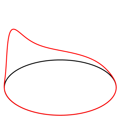
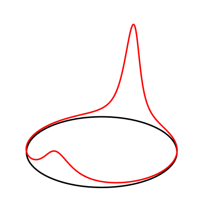
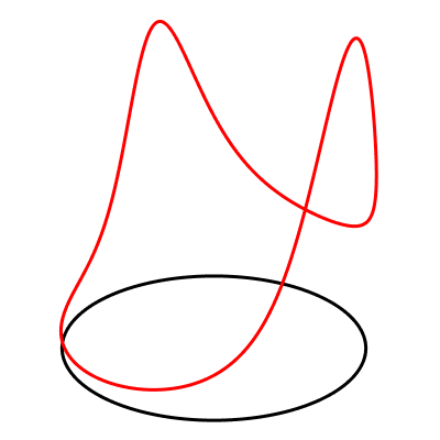
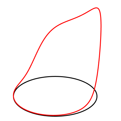
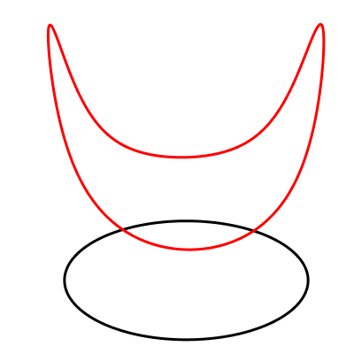
Figure 2: The projected normal density can exhibit asymmetry, bimodality, and antipodality.

Another advantage of this class of distributions is that the connection to the normal distribution enables convenient statistical computation. Considering the static case for a moment, if we observe $\mathbf{u}\sim\textrm{PN}_{n}(\boldsymbol{\mu},\,\boldsymbol{\Sigma})$, we can think of this as a partially observed Gaussian random vector $\mathbf{x}=r\mathbf{u}\sim\textrm{N}_{n}(\boldsymbol{\mu},\,\boldsymbol{\Sigma})$, where the length $r>0$ is an unobserved latent variable. This representation enables classical inference for the parameters $\boldsymbol{\mu}$ and $\boldsymbol{\Sigma}$ via the EM algorithm as in Presnell et al. (1998), and it enables Bayesian inference via a Gibbs sampler that alternates between sampling the parameters and sampling the length, as in Nuñez-Antonio and Gutiérrez-Peña (2005). In this way, the introduction of the latent length functions as a data augmentation in the same spirit as Albert and Chib (1993) for Bayesian probit regression or Diebolt and Robert (1994) for Gaussian mixture models.

In this paper, we combine the computational tractability and distributional flexibility of the projected normal distribution with the tools of dynamic linear models to introduce a state space model that can be applied to spherical time series of arbitrary dimension. The model can be viewed as a partially-observed linear, Gaussian state space model, and this allows us to perform fully Bayesian inference for all of the model’s unobservables (both dynamic latent states and static parameters) using a simple and efficient Gibbs sampler that is based on the familiar Kalman simulation smoother. Leveraging this unique model tractability, we introduce a Rao-Blackwellized particle filter to perform online inference for streaming data. As such, our model is the first with the potential to realize all of the desired properties that previous models have been unable to balance (Table 1). In an application to wind direction data, we find that our model outperforms others in terms of real-time, out-of-sample point, interval, and density forecasting.

2 The model

In order to study the dynamics of a time series on the unit $n$-sphere, we propose the projected dynamic linear model (PDLM):

$$\mathbf{u}_{t}\,|\,\mathbf{s}_{t} \overset{\textrm{indep}}{\sim}\textrm{PN}_{n}\left(\mathbf{F}_{t}\mathbf{s}_{t},\,\boldsymbol{\Sigma}\right)$$ (1)

$$\mathbf{s}_{t} =\mathbf{G}\mathbf{s}_{t-1}+\boldsymbol{\eta}_{t}, \boldsymbol{\eta}_{t}\overset{\textrm{iid}}{\sim}\textrm{N}_{p}(\mathbf{0},\,\mathbf{W})$$ (2)

$$\mathbf{s}_{0} \sim\textrm{N}_{p}\left(\bar{\mathbf{s}}_{0|0},\,\mathbf{P}_{0}\right).$$ (3)

This is a state space model where the observed unit vectors $\mathbf{u}_{t}\in S^{n-1}$ depend on the latent time series $\mathbf{s}_{t}\in\mathbb{R}^{p}$ which we must estimate. The observed and unobserved time series are linked by the measurement distribution in (1), where the projected normal family ensures distributional flexibility, tractable computation, and our ability to handle spherical observations of any dimension $n$. The $n\times p$ matrices $\mathbf{F}_{t}$ are fixed and known, and we can manipulate them to produce different model structures. If we take $p=n$ and all $\mathbf{F}_{t}=\mathbf{I}_{n}$, then the PDLM becomes a signal-in-noise, “local level” type model for spherical time series (see Figure 1). If we take $p=nm$ and set $\mathbf{F}_{t}=\mathbf{I}_{n}\otimes\mathbf{x}_{t}^{\scriptscriptstyle\mathsf{T}}$ for some vector of observed covariates $\mathbf{x}_{t}\in\mathbb{R}^{m}$, then the PDLM becomes a spherical-on-linear regression model like those studied in Presnell et al. (1998) and Nuñez-Antonio et al. (2011), only now $\mathbf{s}_{t}$ can be interpreted as a vector of time-varying regression coefficients.

The model is governed by the static parameters $\boldsymbol{\theta}=(\boldsymbol{\Sigma},\,\mathbf{G},\,\mathbf{W})$, which are typically unknown and must be estimated. The latent state $\mathbf{s}_{t}$ evolves according to the VAR(1) given in (2), and $\mathbf{G}$ and $\mathbf{W}$ determine these dynamics. In some cases we may choose to fix these hyperparameters (like setting $\mathbf{G}=\mathbf{I}_{p}$ for random walk state evolution), but in general we can estimate them, and for convenience we choose a (conditionally) conjugate matrix normal inverse Wishart prior:

$$\mathbf{G},\,\mathbf{W}\sim\textrm{MNIW}_{p,\,p}\left(\nu_{0},\,\boldsymbol{\Psi}_{0},\,\overline{\mathbf{G}}_{0},\,\boldsymbol{\Omega}^{-1}_{0}\right).$$ (4)

We fix the prior hyperparameters to impose the desired amount of shrinkage, and we typically truncate the prior on $\mathbf{G}$ so that it always has eigenvalues inside the unit circle (ensuring $\mathbf{s}_{t}$ is stationary). The parameter $\boldsymbol{\Sigma}$ influences the shape of the measurement distribution, and in general it is not identified because $\textrm{PN}_{n}(\boldsymbol{\mu},\,\boldsymbol{\Sigma})$ and $\textrm{PN}_{n}(c\boldsymbol{\mu},\,c^{2}\boldsymbol{\Sigma})$ are the same distribution for any $c>0$. To ensure identifiability, we impose the following reparametrization and priors due to Hernandez-Stumpfhauser et al. (2017):

$$\boldsymbol{\Sigma} =\begin{bmatrix}\boldsymbol{\Gamma}+\boldsymbol{\gamma}\boldsymbol{\gamma}^{\scriptscriptstyle\mathsf{T}}&\boldsymbol{\gamma}\\ \boldsymbol{\gamma}^{\scriptscriptstyle\mathsf{T}}&1\end{bmatrix},\quad\begin{matrix}\boldsymbol{\Gamma}\sim\textrm{IW}_{n-1}(d_{0},\,\boldsymbol{\Phi}_{0})\\ \boldsymbol{\gamma}\sim\textrm{N}_{n-1}(\bar{\boldsymbol{\gamma}}_{0},\,\boldsymbol{\Lambda}_{0}).\end{matrix}$$ (5)

As in the static case, the key to inference in the PDLM is to augment the “incomplete data” specification in (1, 2, 3) with a latent length variable $r_{t}$ for each observation. This gives the “complete data” or “data-augmented” version of the model:

$$r_{t}\mathbf{u}_{t} =\mathbf{F}_{t}\mathbf{s}_{t}+\boldsymbol{\varepsilon}_{t},\quad\boldsymbol{\varepsilon}_{t}\overset{\textrm{iid}}{\sim}\textrm{N}_{n}\left(\mathbf{0},\,\boldsymbol{\Sigma}\right).$$ (6)

Together with (2, 3), this describes a linear, Gaussian state space model, but the response variable $r_{t}\mathbf{u}_{t}\in\mathbb{R}^{n}$ is only partially observed; we observe $\mathbf{u}_{t}\in S^{n-1}$ but not $r_{t}>0$. So the goal of Bayesian inference is to access the full posterior $p(\mathbf{s}_{0:T},\,r_{1:T},\,\boldsymbol{\theta}\,|\,\mathbf{u}_{1:T})$. Once we have draws from this distribution, the latent lengths are of no independent interest, and they can be discarded so that we are left with a sample from the original PDLM posterior $p(\mathbf{s}_{0:T},\,\boldsymbol{\theta}\,|\,\mathbf{u}_{1:T})$.

To access the data-augmented posterior, we use the Markov chain Monte Carlo (MCMC) sampler described in Algorithm 1. The algorithm is a Gibbs sampler that requires us to iteratively simulate the conditional posterior of each set of unobservables: $\mathbf{s}_{0:T}$, $\boldsymbol{\Gamma}$, $\boldsymbol{\gamma}$, $\mathbf{G}$, $\mathbf{W}$, $r_{1:T}$. Fortunately, this can mostly be done analytically:

• If we condition on both $r_{t}$ and $\mathbf{u}_{t}$, that is the same as saying that we observe the “data” $\mathbf{y}_{t}=r_{t}\mathbf{u}_{t}$. In this case, instead of the model in (6, 2, 3) being a partially-observed linear, Gaussian state space model, it is a fully-observed linear, Gaussian state space model. This means we can access $p(\mathbf{s}_{0:t}\,|\,r_{1:t},\,\boldsymbol{\theta},\,\mathbf{u}_{1:t})$ exactly using the Kalman simulation smoother;

• If we condition on $\mathbf{u}_{t}$, $r_{t}$, and $\mathbf{s}_{t}$, then the quantities $\mathbf{y}_{t}=r_{t}\mathbf{u}_{t}$, $\boldsymbol{\mu}_{t}=\mathbf{F}_{t}\mathbf{s}_{t}$, and $\mathbf{z}_{t}=\mathbf{y}_{t}-\boldsymbol{\mu}_{t}=\begin{bmatrix}\mathbf{z}_{-n,t}&z_{n,t}\end{bmatrix}^{\scriptscriptstyle\mathsf{T}}$ are all observed. From (6) and (5), we see that $\mathbf{z}_{t}\overset{\textrm{iid}}{\sim}\textrm{N}_{n}(\mathbf{0},\,\boldsymbol{\Sigma})$ and $\mathbf{z}_{-n,t}\,|\,z_{n,t}\overset{\textrm{indep}}{\sim}\textrm{N}_{n-1}(\boldsymbol{\gamma}z_{n,t},\,\boldsymbol{\Gamma})$. If we condition on $\boldsymbol{\gamma}$, then $\mathbf{z}_{-n,t}-\boldsymbol{\gamma}z_{n,t}$ is a fully observed, iid sample from a multivariate normal with conjugate inverse Wishart prior on $\boldsymbol{\Gamma}$, and so $p(\boldsymbol{\Gamma}\,|\,\mathbf{s}_{0:T},\,r_{1:T},\,\boldsymbol{\gamma},\,\mathbf{G},\,\mathbf{W},\,\mathbf{u}_{1:T})$ is also inverse Wishart;

• If instead we condition on $\boldsymbol{\Gamma}$, then $\mathbf{z}_{-n,t}\,|\,z_{n,t}\overset{\textrm{indep}}{\sim}\textrm{N}_{n-1}(\boldsymbol{\gamma}z_{n,t},\,\boldsymbol{\Gamma})$ describes a vector-on-scalar regression with known covariance matrix. Given the normal prior on $\boldsymbol{\gamma}$, the conditional posterior $p(\boldsymbol{\gamma}\,|\,\mathbf{s}_{0:T},\,r_{1:T},\,\boldsymbol{\Gamma},\,\mathbf{G},\,\mathbf{W},\,\mathbf{u}_{1:T})$ is also normal with parameters given, for instance, in Koop (2003);

• $p(\mathbf{G},\,\mathbf{W}\,|\,\mathbf{s}_{0:T},\,r_{1:T},\,\boldsymbol{\Gamma},\,\boldsymbol{\gamma},\,\mathbf{u}_{1:T})$ is the posterior of a VAR(1) with a conjugate MNIW prior, where the $\mathbf{s}_{0:T}$ are treated as the data. So it is also MNIW with parameters given, for instance, in Karlsson (2013).

The only conditional posterior that is intractable is that of $r_{1:T}$, but this can be accessed using the slice sampler from Hernandez-Stumpfhauser et al. (2017) that is reproduced in Algorithm 2. With that, a slice-within-Gibbs sampler is given in Algorithm 1 that enables us to conduct fully Bayesian inference for all of the unobservables in the PDLM.

for $p(\mathbf{s}_{0:T}\,|\,r_{1:T},\,\boldsymbol{\Gamma},\,\boldsymbol{\gamma},\,\mathbf{G},\,\mathbf{W},\,\mathbf{u}_{1:T})$ do

       Construct pseudo-data $\mathbf{y}_{t}=r_{t}\mathbf{u}_{t}$ and then draw $\mathbf{s}_{0:T}$ from the posterior of the linear, Gaussian state space model in (6, 2, 3) using an implementation of the Kalman simulation smoother: Durbin and Koopman (2002), Chan and Jeliazkov (2009), etc.

for $p(\boldsymbol{\Gamma}\,|\,\mathbf{s}_{0:T},\,r_{1:T},\,\boldsymbol{\gamma},\,\mathbf{G},\,\mathbf{W},\,\mathbf{u}_{1:T})$ do

       Let $\mathbf{y}_{t}=r_{t}\mathbf{u}_{t}$, $\boldsymbol{\mu}_{t}=\mathbf{F}_{t}\mathbf{s}_{t}$, $\mathbf{z}_{t}=\mathbf{y}_{t}-\boldsymbol{\mu}_{t}=\begin{bmatrix}\mathbf{z}^{\scriptscriptstyle\mathsf{T}}_{-n,t}&z_{n,t}\end{bmatrix}^{\scriptscriptstyle\mathsf{T}}$, and $\mathbf{e}_{t}=\mathbf{z}_{-n,t}-\boldsymbol{\gamma}z_{n,t}$;

      

      Draw $\boldsymbol{\Gamma}\sim\textrm{IW}_{n-1}(d_{T},\,\boldsymbol{\Phi}_{T})$, where $d_{T}=d_{0}+T$ and $\boldsymbol{\Phi}_{T}=\boldsymbol{\Phi}_{0}+\sum\limits_{t=1}^{T}\mathbf{e}_{t}\mathbf{e}_{t}^{\scriptscriptstyle\mathsf{T}}$.

for $p(\boldsymbol{\gamma}\,|\,\mathbf{s}_{0:T},\,r_{1:T},\,\boldsymbol{\Gamma},\,\mathbf{G},\,\mathbf{W},\,\mathbf{u}_{1:T})$ do

       Construct pseudo-data

$$\mathbf{w}=\begin{bmatrix}\mathbf{z}_{-n,1}^{\scriptscriptstyle\mathsf{T}}&\mathbf{z}_{-n,2}^{\scriptscriptstyle\mathsf{T}}&\cdots&\mathbf{z}_{-n,T}^{\scriptscriptstyle\mathsf{T}}\end{bmatrix}^{\scriptscriptstyle\mathsf{T}},\quad\mathbf{v}=\begin{bmatrix}z_{n,1}&z_{n,2}&\cdots&z_{n,T}\end{bmatrix}^{\scriptscriptstyle\mathsf{T}},\quad\mathbf{V}=\mathbf{v}\otimes\mathbf{I}_{n-1}.$$

      Compute

$$\boldsymbol{\Lambda}_{T} =\left[\boldsymbol{\Lambda}_{0}^{-1}+\mathbf{V}^{\scriptscriptstyle\mathsf{T}}\left(\mathbf{I}_{T}\otimes\boldsymbol{\Gamma}^{-1}\right)\mathbf{V}\right]^{-1}$$

$$\bar{\boldsymbol{\gamma}}_{T} =\boldsymbol{\Lambda}_{T}\left[\boldsymbol{\Lambda}_{0}^{-1}\bar{\boldsymbol{\gamma}}_{0}+\mathbf{V}^{\scriptscriptstyle\mathsf{T}}\left(\mathbf{I}_{T}\otimes\boldsymbol{\Gamma}^{-1}\right)\mathbf{w}\right].$$

      Draw $\boldsymbol{\gamma}\sim\textrm{N}_{n-1}\left(\bar{\boldsymbol{\gamma}}_{T},\,\boldsymbol{\Lambda}_{T}\right)$.

for $p(\mathbf{G},\,\mathbf{W}\,|\,\mathbf{s}_{0:T},\,r_{1:T},\,\boldsymbol{\Gamma},\,\boldsymbol{\gamma},\,\mathbf{u}_{1:T})$ do

       Construct pseudo-data $\mathbf{Y}=\begin{bmatrix}\mathbf{s}_{1}&\mathbf{s}_{2}&\cdots&\mathbf{s}_{T}\end{bmatrix}^{\scriptscriptstyle\mathsf{T}}$ and $\mathbf{X}=\begin{bmatrix}\mathbf{s}_{0}&\mathbf{s}_{1}&\cdots&\mathbf{s}_{T-1}\end{bmatrix}^{\scriptscriptstyle\mathsf{T}}$.

      Compute

$$\nu_{T} =\nu_{0}+T$$

$$\boldsymbol{\Omega}_{T} =\mathbf{X}^{\scriptscriptstyle\mathsf{T}}\mathbf{X}+\boldsymbol{\Omega}_{0}$$

$$\overline{\mathbf{G}}_{T} =\boldsymbol{\Omega}_{T}^{-1}(\mathbf{X}^{\scriptscriptstyle\mathsf{T}}\mathbf{Y}+\boldsymbol{\Omega}_{0}\overline{\mathbf{G}}_{0})$$

$$\boldsymbol{\Psi}_{T} =\boldsymbol{\Psi}_{0}+\left(\mathbf{Y}-\mathbf{X}\overline{\mathbf{G}}_{T}\right)^{\scriptscriptstyle\mathsf{T}}\left(\mathbf{Y}-\mathbf{X}\overline{\mathbf{G}}_{T}\right)+\left(\overline{\mathbf{G}}_{T}-\overline{\mathbf{G}}_{0}\right)^{\scriptscriptstyle\mathsf{T}}\boldsymbol{\Omega}_{0}\left(\overline{\mathbf{G}}_{T}-\overline{\mathbf{G}}_{0}\right).$$

      Draw $\mathbf{G},\,\mathbf{W}\sim\textrm{MNIW}_{p,\,p}(\nu_{T},\,\boldsymbol{\Psi}_{T},\,\overline{\mathbf{G}}_{T},\,\boldsymbol{\Omega}^{-1}_{T})$ until $\mathbf{G}$ has eigenvalues in the unit circle.

for $p(r_{1:T}\,|\,\mathbf{s}_{0:T},\,\boldsymbol{\Gamma},\,\boldsymbol{\gamma},\,\mathbf{G},\,\mathbf{W},\,\mathbf{u}_{1:T})$ do

       (parallel) for $t=1,\,2,\,...,\,T$ do

             Draw $r_{t}^{(m)}$ using Algorithm 2 with $r^{(\text{old})}=r_{t}^{(m-1)}$, $\mathbf{u}=\mathbf{u}_{t}$, $\mathbf{m}=\mathbf{F}_{t}\mathbf{s}_{t}$, $\mathbf{S}=\boldsymbol{\Sigma}$.

      

Algorithm 1 Gibbs sampling steps for $p(\mathbf{s}_{0:T},\,r_{1:T},\,\boldsymbol{\Gamma},\,\boldsymbol{\gamma},\,\mathbf{G},\,\mathbf{W}\,|\,\mathbf{u}_{1:T})$

Input: $r^{(\text{old})}$, $\mathbf{u}$, $\mathbf{m}$, $\mathbf{S}$;

Compute $a=\mathbf{u}^{\scriptscriptstyle\mathsf{T}}\mathbf{S}^{-1}\mathbf{u}$ and $b=\mathbf{u}^{\scriptscriptstyle\mathsf{T}}\mathbf{S}^{-1}\mathbf{m}$;

Draw independent $v\sim\textrm{Unif}\left(0,\,\exp\left[-\frac{a}{2}\left(r^{(\text{old})}-\frac{b}{a}\right)^{2}\right]\right)$ and $u\sim\textrm{Unif}(0,\,1)$;

Compute $c=\frac{b}{a}+\max\left\{-\frac{b}{a},\,-\sqrt{\frac{-2\ln v}{a}}\right\}$ and $d=\frac{b}{a}+\sqrt{\frac{-2\ln v}{a}}$;

Return: $r^{(\text{new})}=\left[\left(d^{n}-c^{n}\right)u+c^{n}\right]^{1/n}$.

Algorithm 2 Slice sampling step for $p(r\,|\,\mathbf{u},\,\mathbf{m},\,\mathbf{S})$ when $\mathbf{u}\in S^{n-1}$ and $r\mathbf{u}\sim\textrm{N}_{n}(\mathbf{m},\,\mathbf{S})$

3 Sequential inference

Algorithm 1 describes how to perform “batch” or “offline” inference for the PDLM. In this environment, all of the historical data $\mathbf{u}_{1:T}$ that we wish to analyze are available at once, and we can use our Gibbs sampler to generate full information estimates of all of the PDLM unobservables: both static parameters and dynamic latent states. But because we are modeling time series data, we must also consider the “streaming” or “online” environment where the observations $\mathbf{u}_{t}$ are arriving one-after-another in real-time, and we wish to recursively update our posterior approximation to keep up with the new information. Our Gibbs sampler can be used for this, but it will be very computationally inefficient. When generating a sample from the time $t$ posterior, naive MCMC does not provide a means of recycling the old sample from the time $t-1$ posterior and adjusting it to reflect the influence of the new observation. We must simply rerun the MCMC algorithm from scratch every period, thereby reprocessing all past data. This ignores the fact that time-adjacent posteriors will typically be quite similar, since they differ by only one observation in their conditioning set. Furthermore, if the data are streaming by at high frequency, there may not be enough time between observations to run the MCMC algorithm long enough.

To overcome these issues and perform online inference for streaming data, we propose a particle filter. This algorithm uses importance sampling to recursively construct a weighted Monte Carlo sample from the sequence of data-tempered posteriors. Unlike a naive MCMC approach, this algorithm does recycle and adjust the draws from the previous period in order to avoid reprocessing the entire history of data from scratch. This makes the algorithm much more efficient in terms of clock time per-period than the MCMC algorithm when faced with streaming data. Ideally, our online algorithm would recursively traverse the sequence of full posteriors $p(\mathbf{s}_{0:t},\,r_{1:t},\,\boldsymbol{\theta}\,|\,\mathbf{u}_{1:t})$ just as our MCMC algorithm does in the offline setting. Unfortunately, online inference for both the states and the parameters of a state space model is notoriously difficult in general (Kantas et al., 2015), and we will not confront this issue here. In what follows we will assume that the static parameters $\boldsymbol{\theta}$ are fixed and known, and we henceforth drop them from the notation. Furthermore, while in theory our algorithm targets the sequence of full smoothing distributions $p(\mathbf{s}_{0:t},\,r_{1:t}\,|\,\mathbf{u}_{1:t})$, we only apply it to the filtering problem of recursively approximating the marginal posterior $p(\mathbf{s}_{t},\,r_{t}\,|\,\boldsymbol{\theta},\,\mathbf{u}_{1:t})$. Because of the Markovian structure of the model, this is sufficient for accessing the model’s forecast distribution in real-time.

As with the Gibbs sampler, the inclusion of $r_{t}$ makes the filtering problem challenging, but because of the model’s unique tractability, we will not have to sample it jointly with $\mathbf{s}_{t}$ in the usual way. To see this, consider this marginal-conditional decomposition of the full posterior:

$$p(\mathbf{s}_{0:t},\,r_{1:t}\,|\,\mathbf{u}_{1:t})=p(\mathbf{s}_{0:t}\,|\,r_{1:t},\,\mathbf{u}_{1:t})p(r_{1:t}\,|\,\mathbf{u}_{1:t}).$$ (7)

$p(\mathbf{s}_{0:t},\,r_{1:t}\,|\,\mathbf{u}_{1:t})$ is not tractable, but as we discussed in Section 2, we can access $p(\mathbf{s}_{0:t}\,|\,r_{1:t},\,\mathbf{u}_{1:t})$ exactly via the Kalman filter and smoother. The well-known filtering recursions are restated in Table 2 for convenience. In order, then, to access $p(\mathbf{s}_{0:t},\,r_{1:t}\,|\,\mathbf{u}_{1:t})$, it suffices to access the marginal posterior of the latent lengths $p(r_{1:t}\,|\,\mathbf{u}_{1:t})$. Once we have a sample $\{r_{1:t}^{(m)}\}\sim p(r_{1:t}\,|\,\mathbf{u}_{1:t})$, we can perfectly simulate $\mathbf{s}_{0:t}^{(m)}\sim p(\mathbf{s}_{0:t}\,|\,r_{1:t}^{(m)},\,\mathbf{u}_{1:t})$ to produce draws from the full posterior. This sampling scheme amounts to a Rao-Blackwellization that can improve the Monte Carlo efficiency of the posterior approximation by significantly reducing the dimension of the problem (Robert and Roberts, 2021). Instead of applying Monte Carlo methods to the $(p+1)$-dimensional problem of sampling $\mathbf{s}_{t}$ and $r_{t}$ jointly, we need only apply them to the one dimensional problem of sampling $r_{t}$. The rest of the posterior is handled exactly, with no added Monte Carlo error.

We will use a particle filter to sequentially traverse the sequence of posteriors $p(r_{1:t}\,|\,\mathbf{u}_{1:t})$ as new observations $\mathbf{u}_{t}$ arrive. In order to do this, we need to calculate the unnormalized posterior density. We know that

$$p(r_{1:t}\,|\,\mathbf{u}_{1:t})\propto p(r_{1:t},\,\mathbf{u}_{1:t}),$$ (8)

and in general we know that

$$p(r_{1:t},\,\mathbf{u}_{1:t})=\prod_{k=1}^{t}p(r_{k},\,\mathbf{u}_{k}\,|\,r_{1:k-1},\,\mathbf{u}_{1:k-1}).$$ (9)

From Table 2, we know that

$$p(r_{k}\mathbf{u}_{k}\,|\,r_{1:k-1},\,\mathbf{u}_{1:k-1})=\textrm{N}_{n}(r_{k}\mathbf{u}_{k};\,\bar{\mathbf{y}}_{k|k-1},\,\boldsymbol{\Omega}_{k|k-1}).$$ (10)

If we apply the change of variables $r_{k}\mathbf{u}_{k}\mapsto(r_{k},\,\mathbf{u}_{k})$ from Euclidean to polar coordinates, we get

$$p(r_{k},\,\mathbf{u}_{k}\,|\,r_{1:k-1},\,\mathbf{u}_{1:k-1})=r_{k}^{n-1}\textrm{N}_{n}(r_{k}\mathbf{u}_{k};\,\bar{\mathbf{y}}_{k|k-1},\,\boldsymbol{\Omega}_{k|k-1})q(\mathbf{u}_{k}),$$ (11)

where $q(\cdot)$ is the part of the Jacobian that does not depend on $r_{k}$. Combining (8), (9), and (11), we see that the posterior kernel is

$$p(r_{1:t}\,|\,\mathbf{u}_{1:t})\propto\prod_{k=1}^{t}r_{k}^{n-1}\textrm{N}_{n}(r_{k}\mathbf{u}_{k};\,\bar{\mathbf{y}}_{k|k-1},\,\boldsymbol{\Omega}_{k|k-1}).$$ (12)

Object	Distribution	Details
$\mathbf{s}_{t}\,|\,(r\mathbf{u})_{1:t-1}$	$\textrm{N}_{p}\left(\bar{\mathbf{s}}_{t|t-1},\,\mathbf{P}_{t|t-1}\right)$	$\bar{\mathbf{s}}_{t|t-1}=\mathbf{G}\bar{\mathbf{s}}_{t-1|t-1}$
		$\mathbf{P}_{t|t-1}=\mathbf{G}\mathbf{P}_{t-1|t-1}\mathbf{G}^{\scriptscriptstyle\mathsf{T}}+\mathbf{W}$
$r_{t}\mathbf{u}_{t}\,|\,(r\mathbf{u})_{1:t-1}$	$\textrm{N}_{n}\left(\bar{\mathbf{y}}_{t|t-1},\,\boldsymbol{\Omega}_{t|t-1}\right)$	$\bar{\mathbf{y}}_{t|t-1}=\mathbf{F}_{t}\bar{\mathbf{s}}_{t|t-1}$
		$\boldsymbol{\Omega}_{t|t-1}=\mathbf{F}_{t}\mathbf{P}_{t|t-1}\mathbf{F}_{t}^{\scriptscriptstyle\mathsf{T}}+\boldsymbol{\Sigma}$
$\mathbf{s}_{t}\,|\,(r\mathbf{u})_{1:t}$	$\textrm{N}_{p}\left(\bar{\mathbf{s}}_{t|t},\,\mathbf{P}_{t|t}\right)$	$\bar{\mathbf{s}}_{t|t}=\bar{\mathbf{s}}_{t|t-1}+\mathbf{P}_{t|t-1}\mathbf{F}_{t}^{\scriptscriptstyle\mathsf{T}}\boldsymbol{\Omega}_{t|t-1}^{-1}(r_{t}\mathbf{u}_{t}-\bar{\mathbf{y}}_{t|t-1})$
		$\mathbf{P}_{t|t}=\mathbf{P}_{t|t-1}-\mathbf{P}_{t|t-1}\mathbf{F}_{t}^{\scriptscriptstyle\mathsf{T}}\boldsymbol{\Omega}_{t|t-1}^{-1}\mathbf{F}_{t}\mathbf{P}_{t|t-1}$

Table 2: Kalman filter recursions for updating $\mathbf{K}_{t}$ during the RBPF.

This distribution is not tractable, but we now have a formula for evaluating its unnormalized density pointwise, and that is sufficient to target the sequence with a particle filter. Because our target kernel is the result of having marginalized out the $\mathbf{s}_{t}$, this will be a Rao-Blackwellized particle filter (RBPF) in the sense of Doucet et al. (2000). The goal of a particle filter is to recursively construct a weighted sample $\{r_{1:t}^{(m)},\,W_{t}^{(m)}\}_{m=1}^{M}$ that is adapted to $p(r_{1:t}\,|\,\mathbf{u}_{1:T})$, and as Doucet and Johansen (2011) explain, at the foundation of the method is sequential importance sampling. Given our target kernel

$$k(r_{1:t})=\prod_{k=1}^{t}r_{k}^{n-1}\textrm{N}_{n}(r_{k}\mathbf{u}_{k};\,\bar{\mathbf{y}}_{k|k-1},\,\boldsymbol{\Omega}_{k|k-1}),$$ (13)

and given a sequential importance proposal density

$$g(r_{1:t})=g_{1}(r_{1})\prod_{k=2}^{t}g_{k}(r_{k}\,|\,r_{1:k-1}),$$ (14)

we have the following recursion for the importance weights:

$$W_{t} =\frac{k(r_{1:t})}{g(r_{1:t})}=\frac{k(r_{1:t-1})}{k(r_{1:t-1})}\frac{k(r_{1:t})}{g(r_{1:t})}=\frac{k(r_{1:t-1})}{g(r_{1:t-1})}\frac{k(r_{1:t})}{k(r_{1:t-1})g_{t}(r_{t})}=W_{t-1}\frac{k(r_{1:t})}{k(r_{1:t-1})g_{t}(r_{t})}.$$

Invoking the particular form of $k$, this yields

$$W_{t}=W_{t-1}\frac{r_{t}^{n-1}\textrm{N}_{n}(r_{t}\mathbf{u}_{t};\,\bar{\mathbf{y}}_{t|t-1},\,\boldsymbol{\Omega}_{t|t-1})}{g_{t}(r_{t})}.$$ (15)

We see in (15) that in order to compute the importance weights, we need access to $\bar{\mathbf{y}}_{t|t-1}$ and $\boldsymbol{\Omega}_{t|t-1}$. That is to say, we need access to the Kalman filter output that exactly characterizes the conditional posterior of the state $\mathbf{s}_{t}$. So as we adapt our “swarm” $\{r_{1:t}^{(m)},\,W_{t}^{(m)}\}_{m=1}^{M}$ of particles from period to period, we must also update the statistics that characterize $p(\mathbf{s}_{t}\,|\,r_{1:t}^{(m)},\,\mathbf{u}_{1:t})$. Recalling Table 2, denote these statistics

$$\mathbf{K}_{t}=\left\{\bar{\mathbf{s}}_{t|t-1},\,\mathbf{P}_{t|t-1},\,\bar{\mathbf{y}}_{t|t-1},\,\boldsymbol{\Omega}_{t|t-1},\,\bar{\mathbf{s}}_{t|t},\,\mathbf{P}_{t|t}\right\}.$$ (16)

We can now attach to each particle its own $\mathbf{K}_{t}^{(m)}$ and update them recursively as the algorithm runs. Table 2 describes the map $(\mathbf{K}_{t-1},\,r_{t},\,\mathbf{u}_{t})\mapsto\mathbf{K}_{t}$ that updates the statistics from one period to the next.

With these preliminaries sorted, we give the RBPF in Algorithm 3. Using the language of Chopin (2004), one recursion proceeds in three phases: correction, selection, and mutation. During the correction phase, we propose new values, update the statistics $\mathbf{K}_{t}$, and update the importance weights. A simple choice for $g_{t}$ is a random walk in logs $\text{LogNormal}(\ln r_{t-1},\,\sigma^{2}_{g})$, where $\sigma^{2}_{g}$ is a tuning parameter. In order to prevent the importance weights from degenerating, the selection phase checks whether or not the effective sample size (ESS) of the swarm has dropped below a user-defined threshold $\tau$, and if it has we resample the particles in a multonomial fashion and make the weights uniform. Resampling helps prevent degeneracy in the weights, but at the cost of additional Monte Carlo noise, since the resulting swarm will now contain duplicate values and be less diverse. To combat this, the mutation phase replenishes the particles by “jittering” them according to an MCMC algorithm that targets $p(r_{t}\,|\,r_{1:t-1},\,\mathbf{u}_{1:t})$. For this, we simply recycle the slice sampler in Algorithm 2.

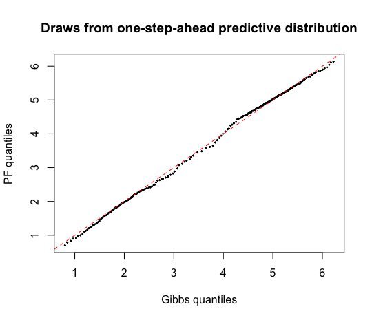
Figure 3: Q-Q plot comparing the draws generated by the Gibbs sampler (Algorithm 1) and the RBPF (Algorithm 3, with ). Given the same priors and data (the wind direction series in Figure 1), they should give similar output.

Given the same data and priors, Algorithm 1 (holding $\boldsymbol{\theta}$ fixed and alternating between the first and last steps) and Algorithm 3 both produce draws from the same posterior distribution. Indeed, Figure 3 is a Q-Q plot comparing the draws from the period $T+1$ predictive distribution that we get when we apply either algorithm to the data in Figure 1. Thankfully, they agree in their output. But these two algorithms are best suited to different data environments. Algorithm 1 is meant for the batch or offline setting where all of the data have arrived and we seek a single good approximation to the time $T$ posterior. Algorithm 3 is meant for the streaming or online setting where we wish to recursively update our posterior approximation as new observations arrive period-after-period in real-time. Algorithm 1 could also be used in this context, but it will be less efficient.

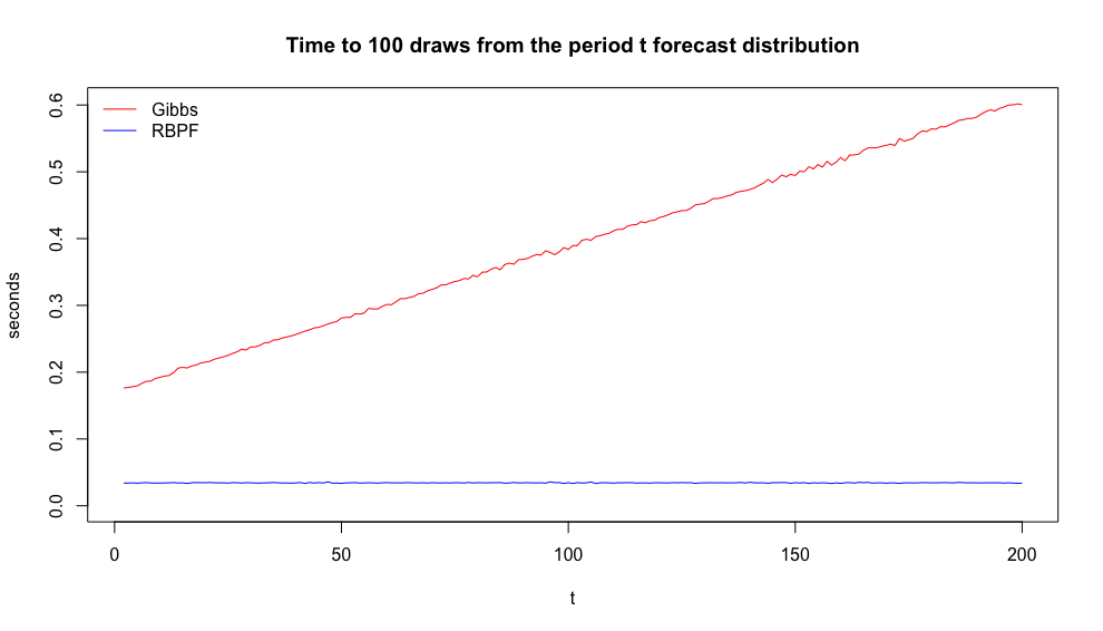
Figure 4: The time in seconds (averaged over ten repetitions) that it takes to generate 100 draws from the forecast distribution $p(\mathbf{u}_{t}\,|\,\mathbf{u}_{1:t-1})$ each period. For the Gibbs sampler this requires reprocessing the entire history of data, so the per-period computing cost scales with the sample size.

Figure 4 displays the time (averaged over ten repetitions) that each algorithm takes to recursively generate one hundred draws from the forecast distribution $p(\mathbf{u}_{t+1}\,|\,\mathbf{u}_{1:t})$ in a simulated dataset. We see that the Gibbs sampler handles this task in $O(t)$ time, whereas the particle filter handles it in $O(1)$ time, which is the signal difference between offline and online inference. The MCMC algorithm is offline because it does not “recycle” the period $t-1$ posterior approximation when it constructs the period $t$ approximation in the way that the RBPF does. When a new observation arrives, the MCMC user must simply rerun their sampler from scratch in order to incorporate the new information. As the sample size grows observation-by-observation, yet more computations will mount as we re-process the entire history of data each period. In a high frequency streaming environment, there may not be time to rerun the MCMC algorithm each period, especially when the time series history is long. In this case, the RBPF is more suitable.

Input: New observation $\mathbf{u}_{t}$; old particles $\left\{\mathbf{K}_{t-1}^{(m)},\,r_{t-1}^{(m)},\,W_{t-1}^{(m)}\right\}_{m=1}^{M}$ adapted to $p(r_{t-1}\,|\,\mathbf{u}_{1:t-1})$;

for  (Correction)  do

      

      (parallel) for $m=1,,\,2,\,...,\,M$ do

             Propose $\tilde{r}_{t}^{(m)}\sim g_{t}(r_{t}\,|\,r_{t-1}^{(m)},\,...)$;

             Update $\left(\mathbf{K}_{t-1}^{(m)},\,\tilde{r}_{t}^{(m)},\,\mathbf{u}_{t}\right)\mapsto\tilde{\mathbf{K}}_{t}^{(m)}$ using Table 2;

             Reweight

$$\tilde{W}_{t}^{(m)}\propto W_{t-1}^{(m)}\frac{\left[\tilde{r}^{(m)}_{t}\right]^{n-1}\textrm{N}_{n}\left(\tilde{r}^{(m)}_{t}\mathbf{u}_{t};\,\bar{\mathbf{y}}^{(m)}_{t|t-1},\,{\boldsymbol{\Omega}}^{(m)}_{t|t-1}\right)}{g_{t}\left(\tilde{r}^{(m)}_{t}\right)};$$

      

for  (Selection)  do

       Compute $\text{ESS}=M/\left(M^{-1}\sum\limits_{m=1}^{M}\left[\tilde{W}_{t}^{(m)}\right]^{2}\right)^{-1}$;

       for $m=1,,\,2,\,...,\,M$ do

             if $\text{ESS}<\tau$ then

                   Draw $(\mathbf{K}_{t}^{(m)},\,r_{t}^{(m)})\sim\{\tilde{\mathbf{K}}_{t}^{(j)},\,\tilde{r}_{t}^{(j)},\,\tilde{W}_{t}^{(j)}\}_{j=1}^{M}$;

                   Set $W_{t}^{(m)}=1/M$;

                  

            else

                   Set $(\mathbf{K}_{t}^{(m)},\,r_{t}^{(m)},\,W_{t}^{(m)})=(\tilde{\mathbf{K}}_{t}^{(m)},\,\tilde{r}_{t}^{(m)},\,\tilde{W}_{t}^{(m)})$;

                  

            

      

for (Mutation) do

       (parallel) for $m=1,,\,2,\,...,\,M$ do

             Mutate $r_{t}^{(m)}$ for $L$ iterations of Algorithm 2 with $\mathbf{u}=\mathbf{u}_{t}$, $\mathbf{m}=\bar{\mathbf{y}}^{(m)}_{t|t-1}$, $\mathbf{S}=\boldsymbol{\Omega}_{t|t-1}^{(m)}$;

             Update $\bar{\mathbf{s}}_{t|t}^{(m)}$ in $\mathbf{K}^{(m)}_{t}$ based on the final value of $r_{t}^{(m)}$.

      

Return: New particles $\left\{\mathbf{K}_{t}^{(m)},\,r_{t}^{(m)},\,W_{t}^{(m)}\right\}_{m=1}^{M}$ adapted to $p(r_{t}\,|\,\mathbf{u}_{1:t})$.

Algorithm 3 Rao-Blackwellized particle filter for $p(r_{t}\,|\,\boldsymbol{\Gamma},\,\boldsymbol{\gamma},\,\mathbf{G},\,\mathbf{W},\,\mathbf{u}_{1:t})$

4 Forecasting with the PDLM

We take a Bayesian approach to forecasting. The PDLM (and all of the other models introduced in Section 5) are equipped with a prior $p(\boldsymbol{\phi})$ over the static and dynamic unobservables $\boldsymbol{\phi}$ and a likelihood increment $p(\mathbf{u}_{t+1}\,|\,\mathbf{u}_{1:t},\,\boldsymbol{\phi})$ that describes the time series dynamics. In the case of the PDLM for example, we have $\boldsymbol{\phi}=\{\mathbf{s}_{0:T},\,r_{1:T},\,\boldsymbol{\Gamma},\,\boldsymbol{\gamma},\,\mathbf{G},\,\mathbf{W}\}$, and $p(\mathbf{u}_{t+1}\,|\,\mathbf{u}_{1:t},\,\boldsymbol{\phi})$ is implied by (1). The posterior distribution $p(\boldsymbol{\phi}\,|\,\mathbf{u}_{1:t})$ is given by Bayes’ theorem, and once we have it, we are interested in accessing the one-step-ahead posterior predictive distribution:

$$p(\mathbf{u}_{t+1}\,|\,\mathbf{u}_{1:t})=\int p(\mathbf{u}_{t+1}\,|\,\mathbf{u}_{1:t},\,\boldsymbol{\phi})p(\boldsymbol{\phi}\,|\,\mathbf{u}_{1:t})\,\textrm{d}\boldsymbol{\phi}.$$

In order to do this, we first generate a sample from the posterior distribution $\{\boldsymbol{\phi}^{(j)}\}_{j=1}^{J}\sim p(\boldsymbol{\phi}\,|\,\mathbf{u}_{1:t})$, and then we simulate the model forward on a per-draw basis in order to produce a sample from the predictive distribution $\{\tilde{\mathbf{u}}^{(j)}_{t+1}\}_{j=1}^{J}\sim p(\mathbf{u}_{t+1}\,|\,\mathbf{u}_{1:t})$. In this section we explain how to post-process this Monte Carlo output in order to produce and evaluate point, interval, and density forecasts. In particular, we focus on the circular case where we can reparametrize $\tilde{a}_{t+1}=\text{atan2}(\tilde{\mathbf{u}}_{t+1})\text{ mod }2\pi$.

4.1 Point forecasting

To generate a point forecast, we can calculate a circular summary statistic for the draws $\{\tilde{a}^{(j)}_{t+1}\}_{j=1}^{J}$, such as the sample mean direction or the sample circular median. We opt for the latter, which is given by

$$\hat{a}_{t+1|t}^{(\text{med})}=\underset{0\leq a<2\pi}{\arg\min}\left(\pi-\sum\limits_{j=1}^{J}\left|\pi-\left|\tilde{a}_{t+1}^{(j)}-a\right|\right|\right),$$ (17)

and can be calculated using the circular package in R. We can measure the error between a forecast $\hat{a}$ and a realization $a$ with circular distance $d(a,\,\hat{a})=1-\cos(a-\hat{a})$, and so given a sequence of point forecasts $\hat{a}_{t|t-1}$ and subsequent realizations $a_{t}$, the mean circular error of a method is

$$\textrm{MCE}=\frac{1}{T-t_{0}}\sum\limits_{t=t_{0}}^{T}[1-\cos(a_{t}-\hat{a}_{t|t-1})].$$ (18)

4.2 Interval forecasting

We construct interval forecasts based on the quantiles of the forecast distribution. We approximate these using the sample circular quantiles of the Monte Carlo draws $\{\tilde{a}^{(j)}_{t+1}\}_{j=1}^{J}$, which can be computed using the circular package in R. Since the circle is not endowed with an order in the same way that the real line is, the “quantiles” of a circular distribution are calculated in relation to its circular median, which was given in (17). Essentially, we linearize the circular sample about the median, calculate ordinary sample quantiles, and then transform them back to the circular scale. Algorithm 4 gives the details of this calculation, and Figure 5 displays the steps.

Input: $\alpha\in(0,\,1)$, $\{x_{1},\,x_{2},\,...,\,x_{n}\}\subseteq[0,\,2\pi)$;

Compute sample circular median $m=\underset{0\leq a<2\pi}{\arg\min}\left(\pi-\sum\limits_{i=1}^{n}\left|\pi-\left|x_{i}-a\right|\right|\right)$;

Calculate $y_{i}=(x_{i}-m)\text{ mod }2\pi$ for each $i=1,\,2,\,...,\,n$;

If $y_{i}>\pi$, replace $y_{i}\leftarrow y_{i}-2\pi$;

Calculate ordinary $\alpha$th sample quantile $r(\alpha)$ of $\{y_{1},\,y_{2},\,...,\,y_{n}\}$;

Return: $q(\alpha)=[r(\alpha)+m]\text{ mod }2\pi$.

Algorithm 4 Calculate $\alpha$th sample circular quantile

Given a coverage level $1-\alpha$ and the sample circular quantiles $\tilde{q}_{t+1}(\alpha/2)$ and $\tilde{q}_{t+1}(1-\alpha/2)$ of the $\{\tilde{a}^{(j)}_{t+1}\}_{j=1}^{J}$, we consider set forecasts of the form

$$I_{t+1|t}(\alpha)=\begin{cases}[\tilde{q}_{t+1}(\alpha/2),\,\tilde{q}_{t+1}(1-\alpha/2)]&\tilde{q}_{t+1}(\alpha/2)\leq\tilde{q}_{t+1}(1-\alpha/2)\\ [0,\,\tilde{q}_{t+1}(1-\alpha/2)]\cup[\tilde{q}_{t+1}(\alpha/2),\,2\pi]&\tilde{q}_{t+1}(1-\alpha/2)<\tilde{q}_{t+1}(\alpha/2).\end{cases}$$ (19)

As we see in the first panel of Figure 5, it is possible for the quantiles to “wrap around” the interval $[0,\,2\pi)$ and not be ordered in the same way that ordinary, linear quantiles would be, so our definition adjusts for this. We evaluate the real-time performance of these set forecasts by calculating the mean interval length and the empirical coverage

MIL $$=\frac{1}{T-t_{0}}\sum\limits_{t=t_{0}}^{T}\textrm{length}\left(I_{t|t-1}(\alpha)\right)$$ (20)

EC $$=\frac{1}{T-t_{0}}\sum\limits_{t=t_{0}}^{T}1\{a_{t}\in I_{t|t-1}(\alpha)\},$$ (21)

where

$$\textrm{length}\left(I_{t|t-1}(\alpha)\right)=\begin{cases}\tilde{q}_{t}(1-\alpha/2)-\tilde{q}_{t}(\alpha/2)&\tilde{q}_{t}(\alpha/2)\leq\tilde{q}_{t}(1-\alpha/2)\\ 2\pi-[\tilde{q}_{t}(\alpha/2)-\tilde{q}_{t}(1-\alpha/2)]&\tilde{q}_{t}(1-\alpha/2)<\tilde{q}_{t}(\alpha/2).\end{cases}$$ (22)

A method performs well if it delivers high coverage intervals of modest size.

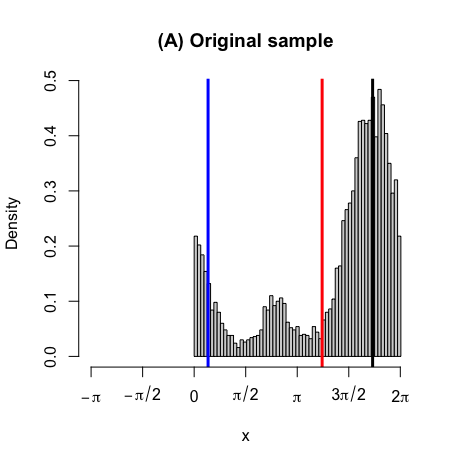
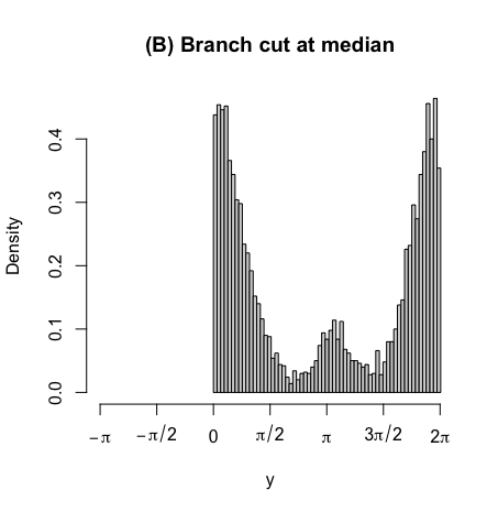
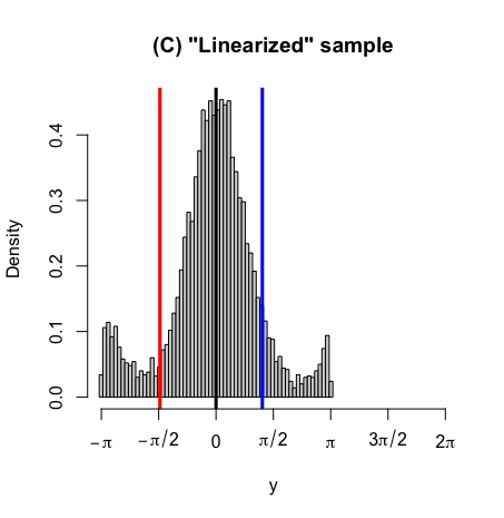
Figure 5: 0.1, 0.5, and 0.9 quantiles in red, black, and blue. Panel (A) displays the original $x_{i}$ and their sample circular quantiles. Panel (B) displays the $y_{i}=(x_{i}-m)\text{ mod }2\pi$. Panel (C) displays the change $[0,\,2\pi)\to[-\pi,\,\pi)$ and the sample quantiles of the final linearized sample.

4.3 Density forecasting

The sample $\{\tilde{a}^{(j)}_{t+1}\}_{j=1}^{J}$ represents a discrete approximation of the forecast distribution $p(a_{t+1}\,|\,a_{1:t})$, so to score the distribution forecast as a whole, we use the circular continuous ranked probability score (CRPS) of Grimit et al. (2006). If $F$ is a forecast distribution and $a$ the subsequent realization, then

$$\textrm{CRPS}\left(F,\,a\right)=E\left[d(\tilde{a},\,a)\right]-\frac{1}{2}E\left[d(\tilde{a},\,\tilde{a}^{\prime})\right],\quad\tilde{a},\,\tilde{a}^{\prime}\overset{\textrm{iid}}{\sim}F.$$ (23)

In the case where $F$ is represented by the Monte Carlo sample $\{\tilde{a}^{(j)}_{t}\}_{j=1}^{J}$, we approximate the CRPS with

$$\textrm{CRPS}\left(\{\tilde{a}^{(j)}_{t}\},\,a_{t}\right)=\frac{1}{J}\sum\limits_{j=1}^{J}d(\tilde{a}_{t}^{(j)},\,a_{t})-\frac{1}{2}\frac{1}{J^{2}}\sum\limits_{j=1}^{J}\sum\limits_{k=1}^{J}d(\tilde{a}_{t}^{(j)},\,\tilde{a}_{t}^{(k)}).$$ (24)

This can be computed using the CircSpaceTime package in R (Jona Lasinio et al., 2020). To score the entire path of forecast distributions over time, we calculate each method’s mean CRPS:

$$\textrm{MCRPS}=\frac{1}{T-t_{0}}\sum\limits_{t=t_{0}}^{T}\textrm{CRPS}\left(\{\tilde{a}^{(j)}_{t}\},\,a_{t}\right).$$ (25)

The smaller the MCRPS is, the better the forecast distributions are on average.

5 Application: forecasting wind direction

The PDLM can be applied to time series on a unit sphere of arbitrary dimension $n$, but most competing models are limited to the special case of circular data ($n=2$). As such, we will demonstrate the performance of the PDLM by comparing its out-of-sample predictive performance to a portfolio of alternative models in the case of forecasting wind direction. In this setting, our circular data $\mathbf{u}_{t}\in S^{1}$ can alternatively be written as an angle $a_{t}\in[0,\,2\pi)$. All of the competing models handle circular data in this form.

5.1 Competing models

5.1.1 Naive methods

The first set of approaches we compare to are naive methods that simply apply familiar linear, Gaussian models to an observed time series of angles $a_{1:T}$ with no regard at all for the special circular structure of the data. Because the unit circle is locally Euclidean, if the time series only varies in a small region of the circle, applying linear methods may work well enough. The first model is an ordinary AR($p$)

$$a_{t} =\beta_{0}+\sum\limits_{l=1}^{p}\beta_{l}a_{t-l}+\varepsilon_{t},\quad\varepsilon_{t}\overset{\textrm{iid}}{\sim}\textrm{N}(0,\,\sigma^{2})$$ (26)

with a conjugate normal-inverse-gamma prior on $\boldsymbol{\beta}$ and $\sigma^{2}$. The second model is a local level dynamic linear model (DLM)

$$a_{t} =s_{t}+\varepsilon_{t}, \varepsilon_{t}\overset{\textrm{iid}}{\sim}\textrm{N}(0,\,v)$$ (27)

$$s_{t} =s_{t-1}+\eta_{t}, \eta_{t}\overset{\textrm{iid}}{\sim}\textrm{N}(0,\,w)$$ (28)

with independent normal and inverse gamma priors on $s_{0}$, $v$, and $w$. Because these models ignore the circular structure of the data, they can generate forecasts outside the interval $[0,\,2\pi)$. But because we are fitting these models from a Bayesian point of view, we can base our forecasts on the wrapped posterior predictive distribution $p(a_{t+1}\text{ mod }2\pi\,|\,a_{1:t})$. In the end, this will not help very much.

5.1.2 Classical circular methods

Next we compare with the “first generation” of circular time series models that are summarized in Fisher and Lee (1994). The first is the wrapped autoregression of order $p$, or WAR($p$), which treats our circular time series as a wrapped version of a latent linear time series that has to be inferred:

$$a_{t} =x_{t}\text{ mod }2\pi$$ (29)

$$x_{t} =b_{0}+\sum\limits_{l=1}^{p}b_{l}x_{t-l}+\varepsilon_{t},\quad\varepsilon_{t}\overset{\textrm{iid}}{\sim}\textrm{N}(0,\,\tau^{2}).$$ (30)

If we place a normal-inverse-gamma prior on $(\mathbf{b},\,\tau^{2})$, then we can access $p(\mathbf{b},\,\tau^{2},\,x_{1:T}\,|\,a_{1:T})$ with a Metropolis-within-Gibbs algorithm that alternates between drawing from $p(\mathbf{b},\,\tau^{2}\,|\,x_{1:T},\,a_{1:T})$ exactly, and drawing from $p(x_{1:T}\,|\,\mathbf{b},\,\tau^{2},\,a_{1:T})$ using the Metropolis-Hastings algorithm described in Coles (1998). The second model is the linked autoregression of order $p$, or LAR($p$),

$$a_{t}\,|\,a_{t-1},\,...,\,a_{t-p} \sim\textrm{vM}\left(g\left(\psi_{0}+\sum\limits_{l=1}^{p}\psi_{l}h^{-1}\left(a_{t-l}\right)\right),\,\kappa\right),$$ (31)

where vM(…) denotes the von Mises distribution and $h:(-\pi,\,\pi)\to\mathbb{R}$ is any odd, monotone function with $h(0)=0$, such as $2\tan^{-1}x$. We place independent normal and inverse gamma priors on $\boldsymbol{\psi}=[\psi_{0}\,\psi_{1}\,\cdots\psi_{p}]^{\scriptscriptstyle\mathsf{T}}$ and $\kappa$, and we sample from the posterior using Stan (Carpenter et al., 2017).

5.1.3 Approximate state space methods

Kurz et al. (2016a) review many possible model configurations, but a simple example is this “additive” model based on the wrapped normal distribution, which we abbreviate WN-SSM:

$$a_{t} =(s_{t}+\varepsilon_{t})\text{ mod }2\pi, \varepsilon_{t}\overset{\textrm{iid}}{\sim}\textrm{WN}(0,\,\sigma^{2})$$ (32)

$$s_{t} =(s_{t-1}+\eta_{t})\text{ mod }2\pi, \eta_{t}\overset{\textrm{iid}}{\sim}\textrm{WN}(0,\,\tau^{2}).$$ (33)

We also consider the model from Kurz et al. (2016b), which we abbreviate vMF-SSM:

$$\mathbf{u}_{t}\,|\,\mathbf{s}_{t} \overset{\textrm{indep}}{\sim}\textrm{vMF}_{n}(\mathbf{s}_{t},\,\kappa)$$ (34)

$$\mathbf{s}_{t}\,|\,\mathbf{s}_{t-1} \sim\textrm{vMF}_{n}(\mathbf{s}_{t-1},\,\eta).$$ (35)

$\textrm{vMF}_{n}(...)$ denotes the von Mises-Fisher distribution. This model distinguishes itself as the first in our portfolio that readily generalizes to the case of $n>2$, although it does so with recourse to the von Mises-Fisher distribution, which is not as flexible as the projected normal. Closed-form filtering and smoothing recursions are unavailable for these models, but the Matlab toolbox libDirectional (Kurz et al., 2019) provides routines for approximate filtering based on unscented transformations and deterministic sampling. Lacking a means of estimating the static parameters $\sigma^{2}$, $\tau^{2}$, $\kappa$, and $\eta$, we set them to one.

5.2 Forecasting wind direction on Black Mountain, Australia

To evaluate the performance of the PDLM, we perform a recursive, one-step-ahead forecasting exercise based on the Black Mountain wind direction data in Figure 1. For each $t=10,\,...,\,T-1$, we train all of our models on the data up to period $t$, and then generate the point, interval, and density forecasts for period $t+1$. We compare the forecasts to the subsequent realizations of $a_{t+1}$, and we average the forecasting performance over time for each model. The results are summarized in Table 3.

In terms of point forecasting, the best methods are the state space models from Kurz et al. (2016a) and the PDLM. The PDLM beats all models except for the vMF state space model, which is only slightly better. The interval forecasts were based on 90% Bayesian credible sets, and we see that the PDLM gives the smallest forecast sets of any method, with close to nominal coverage. The approximate state space models give forecast sets with higher coverage, but the sets are twice as large. Lastly, the PDLM is the clear winner in terms of density forecasting, with the smallest mean CRPS. So in a context where data are plentiful and several alternative methods have been proposed, we see that the PDLM delivers better overall forecasting performance than its competitors. It is important to note the poor overall performance of naive methods like the ordinary DLM and autoregression. This reinforces the point illustrated in Figure 1 that it is generally necessary to apply methods to spherical data that actually respect their special structure. In this way, we see that the wrapped and linked autoregressions perform fairly well, with next-best CRP scores, high coverage intervals of modest size, and decent point forecasting performance. Unfortunately, recalling Table 1, these models do not extend past the case of $n=2$, hampering their usefulness in general.

	MCE (18)	length (20)	coverage (21)	MCRPS (25)
DLM	0.408	4.891	0.952	0.368
AR($p=1$)	0.496	3.491	0.774	0.398
WAR($p=1$)	0.268	3.025	0.919	0.233
LAR($p=1$)	0.320	3.899	0.935	0.285
WN-SSM	0.262	4.995	0.952	0.330
vMF-SSM	0.246	5.453	0.968	0.417
PDLM	0.250	2.251	0.871	0.218

Table 3: One-step-ahead, out-of-sample forecasting metrics for the Black Mountain data. The PDLM generates competitive point forecasts, the smallest forecast intervals with near nominal coverage, and the best density forecasts.

6 Conclusion

In Section 5 we saw that to model time series on $S^{n-1}$, it does not suffice to ignore the special structure of the data and apply ordinary linear, Gaussian methods. We can greatly improve predictive accuracy by using models that are tailored to data on $S^{n-1}$. There have been several such models proposed for the special case of $n=2$, but very few for the more general case of $n>2$, and little of this work has been from the Bayesian point of view. In this paper we proposed a state space model based on the projected normal distribution that can model spherical time series of arbitrary dimension, and we described how to perform fully Bayesian inference in this model using an MCMC algorithm for offline inference, and an RBPF for online inference. In a classic application to wind direction forecasting, we show that the proposed model outperforms its many competitors in terms of point, interval, and density prediction. In this comparison we restricted ourselves to a circular example ($n=2$) because that is the case for which most alternative methods (with attendant software) have been developed. Furthermore, we only considered the “local level” ($\mathbf{F}_{t}=\mathbf{I}_{n}$) variant of the model. In future work we will explore applications in the spherical setting ($n>2$), as well as applications of other model variants, such as the dynamic regression model ($\mathbf{F}_{t}=\mathbf{I}_{n}\otimes\mathbf{x}_{t}^{\scriptscriptstyle\mathsf{T}}$).

Appendix A Calculating the trend in the local-level PDLM

Figure 1 displays an estimate of “trend” for the local-level version ($\mathbf{F}_{t}=\mathbf{I}_{n}$) of the PDLM. This is the mean direction $\mathbf{m}_{t}=E(\mathbf{u}_{t}\,|\,\mathbf{s}_{t},\,\boldsymbol{\Sigma})/||E(\mathbf{u}_{t}\,|\,\mathbf{s}_{t},\,\boldsymbol{\Sigma})||_{2}$, which is not equal to $\mathbf{s}_{t}$. It is a posterior functional of $\mathbf{s}_{t}$ and $\boldsymbol{\Sigma}$ that is difficult to calculate exactly in the general case (Wang and Gelfand, 2013). As such, we approximate the functional using Monte Carlo integration, as described in Algorithm 5. Given posterior samples of $\mathbf{s}_{t}$ and $\boldsymbol{\Sigma}$, we can apply Algorithm 5 on a draw-by-draw basis to produce posterior samples of the mean direction $\mathbf{m}_{t}$. Summaries of these draws are what is displayed in Figure 1.

Input: $\mathbf{s}$, $\boldsymbol{\Sigma}$, $L$;

Simulate $\tilde{\mathbf{u}}_{1},\,\tilde{\mathbf{u}}_{2},\,...,\,\tilde{\mathbf{u}}_{L}\overset{\textrm{iid}}{\sim}\text{PN}_{n}(\mathbf{s},\,\boldsymbol{\Sigma})$;

Calculate $\bar{\mathbf{u}}=\sum_{l=1}^{L}\tilde{\mathbf{u}}_{l}/L$;

Return: $\bar{\mathbf{u}}/||\bar{\mathbf{u}}||_{2}$.

(Option: if $n=2$, return $\text{atan2}(\bar{\mathbf{u}})\text{ mod }2\pi$)

Algorithm 5 Approximate the mean direction $E(\mathbf{u})/||E(\mathbf{u})||_{2}$ of $\mathbf{u}\sim\text{PN}_{n}(\mathbf{s},\,\boldsymbol{\Sigma})$

Appendix B Simulation: Algorithm 1 “gets it right”

In order to provide evidence that Algorithm 1 has the correct invariant distribution and has been implemented correctly in the computer, we apply the check from Geweke (2004). The main idea behind Geweke (2004) is that our Bayesian model specifies a joint distribution for both observables and unobservables:

$$p(\mathbf{u}_{1:T},\,r_{1:T},\,\mathbf{s}_{0:T},\,\boldsymbol{\theta})=\underbrace{p(\mathbf{u}_{1:T},\,r_{1:T}\,|\,\mathbf{s}_{0:T},\,\boldsymbol{\theta})}_{(\ref{eq:measurement2})}\underbrace{p(\mathbf{s}_{0:T}\,|\,\boldsymbol{\theta})}_{(\ref{eq:transition},\,\ref{eq:initialization1})}\underbrace{p(\boldsymbol{\theta})}_{(\ref{eq:gw},\,\ref{eq:sig})}.$$

This joint distribution can be simulated in two ways:

• (marginal-conditional sampler) first sample $p(\boldsymbol{\theta})$ from (4, 5), then $p(\mathbf{s}_{0:T}\,|\,\boldsymbol{\theta})$ from (2, 3), then $p(\mathbf{u}_{1:T},\,r_{1:T}\,|\,\mathbf{s}_{0:T},\,\boldsymbol{\theta})$ from (6). This is a direct sampler that generates iid draws from the joint distribution;

• (successive-conditional sampler) alternate between sampling the conditional distributions $p(r_{1:T},\,\mathbf{s}_{0:T},\,\boldsymbol{\theta}\,|\,\mathbf{u}_{1:T})$ and $p(\mathbf{u}_{1:T}\,|\,r_{1:T},\,\mathbf{s}_{0:T},\,\boldsymbol{\theta})$. This is a Gibbs sampler that generates serially correlated draws from the joint distribution. The first conditional is the usual posterior distribution that is targeted by our MCMC algorithm. The second conditional is the model likelihood (which is implicit in our case).

The marginal-conditional sampler is straightforward to implement using standard software. The successive-conditional sampler depends on the implementation of our MCMC algorithm. If everything (including the MCMC algorithm) has been implemented correctly, then the two samplers should generate draws from the same distribution, and we can verify this using probability plots or a statistical test. Furthermore, if we can conclude that Algorithm 1 has been implemented correctly, we can directly compare its output to that of Algorithm 3 (as we did in Figure 3), which provides evidence that our particle filter has also been implemented correctly.

Implementing this check requires that we sample from $p(\mathbf{u}_{1:T}\,|\,r_{1:T},\,\mathbf{s}_{0:T},\,\boldsymbol{\theta})$, which is difficult in general. However, in the special case with $n=2$ and $\boldsymbol{\Sigma}=\mathbf{I}_{2}$, it is possible. First, we reparametrize the unit vector observation $\mathbf{u}_{t}$ as $\mathbf{u}_{t}=[\cos a_{t}\,\sin a_{t}]^{\scriptscriptstyle\mathsf{T}}$ for some $a_{t}\in[0,\,2\pi)$, and we set $\boldsymbol{\mu}_{t}=\mathbf{F}_{t}\mathbf{s}_{t}$. We see in (6) that the measurement distribution of the data-augmented state-space model is then

$$r_{t}\mathbf{u}_{t}=r_{t}\begin{bmatrix}\cos a_{t}\\ \sin a_{t}\end{bmatrix}\sim\textrm{N}_{2}\left(\boldsymbol{\mu}_{t}=\begin{bmatrix}\mu_{t}^{(1)}\\ \mu_{t}^{(2)}\end{bmatrix},\,\mathbf{I}_{2}\right).$$

Applying a change-of-variables to polar coordinates, we can rewrite the measurement density as

$$p(r_{t},\,a_{t}\,|\,\boldsymbol{\mu}_{t})=\frac{r_{t}}{2\pi}\exp\left(-\frac{1}{2}\left[\left(r_{t}\cos a_{t}-\mu_{t}^{(1)}\right)^{2}+\left(r_{t}\sin a_{t}-\mu_{t}^{(2)}\right)^{2}\right]\right).$$

So the conditional density for $a_{t}$ is

$$p(a_{t}\,|\,r_{t},\,\boldsymbol{\mu}_{t})=\frac{p(r_{t},\,a_{t}\,|\,\boldsymbol{\mu}_{t})}{\int_{0}^{2\pi}p(r_{t},\,a_{t}\,|\,\boldsymbol{\mu}_{t})\,\textrm{d}a_{t}}=\frac{\exp\left(r_{t}\mu_{t}^{(1)}\cos a_{t}+r_{t}\mu_{t}^{(2)}\sin a_{t}\right)}{2\pi I_{0}(r_{t}||\boldsymbol{\mu}_{t}||_{2})},$$ (36)

where $I_{0}$ is the modified Bessel function of order 0. When $r_{t}=1$ and $\boldsymbol{\mu}_{t}=[\cos\lambda\,\sin\lambda]^{\scriptscriptstyle\mathsf{T}}$ for some $\lambda\in[0,\,2\pi)$, then this is the density of the von Mises distribution with location paramater $\lambda$ and concentration parameter $\kappa=1$. We can show that

$$M=\max_{0<a_{t}<2\pi}\frac{p(a_{t}\,|\,r_{t},\,\boldsymbol{\mu}_{t})}{1/2\pi}=\frac{\exp\left(r_{t}||\boldsymbol{\mu}_{t}||_{2}\right)}{I_{0}(r_{t}||\boldsymbol{\mu}_{t}||_{2})},$$

and this enables us to implement Algorithm 6 to sample directly from $p(a_{t}\,|\,r_{t},\,\boldsymbol{\mu}_{t})$. Figure 6 displays a histogram of draws from Algorithm 6 and a line plot of the density in (36), and they clearly agree. Because the $\mathbf{u}_{1:T}$ are conditionally independent given the $\mathbf{s}_{0:T}$ and $r_{1:T}$, we can sample from $p(\mathbf{u}_{1:T}\,|\,r_{1:T},\,\mathbf{s}_{0:T},\,\boldsymbol{\theta})$ by separately applying Algorithm 6 for each $t$.

Input: $r$, $\boldsymbol{\mu}$;

Calculate $M=\exp\left(r||\boldsymbol{\mu}||_{2}\right)/I_{0}(r||\boldsymbol{\mu}||_{2})$;

Draw $U\sim\textrm{Unif}(0,\,1)$;

Propose $V\sim\textrm{Unif}(0,\,2\pi)$;

while $U\geq 2\pi p(V\,|\,r,\,\boldsymbol{\mu})/M$ do

       Draw $U\sim\textrm{Unif}(0,\,1)$;

       Propose $V\sim\textrm{Unif}(0,\,2\pi)$;

      

Return: $V$.

Algorithm 6 Accept-reject sampler for $p(a\,|\,r,\,\boldsymbol{\mu})$ when $\begin{bmatrix}r\cos a&r\sin a\end{bmatrix}^{\scriptscriptstyle\mathsf{T}}\sim\text{N}_{2}(\boldsymbol{\mu},\,\mathbf{I}_{2})$

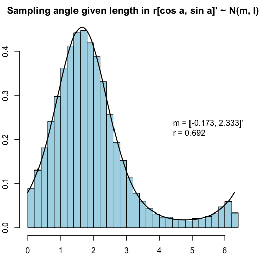
Figure 6: A histogram of draws from Algorithm 6 agrees with the density in (36).

With this, we apply Geweke (2004) with the following settings:

• $n=2$; $p=3$; $T=5$; $\boldsymbol{\Sigma}=\mathbf{I}_{n}$; each $\mathbf{F}_{t}$ filled with iid draws from $\text{N}(0,\,1)$;

• $\bar{\mathbf{s}}_{1|0}=\mathbf{0}$; $\mathbf{P}_{1|0}=\mathbf{I}_{p}$; $\nu_{0}=p+2$; $\boldsymbol{\Psi}_{0}=\mathbf{I}_{p}$; $\overline{\mathbf{G}}_{0}=\mathbf{0}$; $\boldsymbol{\Omega}^{-1}_{0}=\mathbf{I}_{p}$;

• 5,000 draws from each sampler; the successive-conditional draws thinned down from 50,000.

Lastly, note that because we are fixing $\boldsymbol{\Sigma}=\mathbf{I}_{n}$, we are testing the special case of Algorithm 1 that skips the steps for $\boldsymbol{\Gamma}$ and $\boldsymbol{\gamma}$. With that, Figure 7 displays Q-Q plots comparing the draws from the marginal-conditional sampler (horizontal axis) to the draws from the successive-conditional sampler (vertical axis) for a selection of observables and unobservables in the PDLM. In all cases, we see that the Q-Q points lie on the 45 degree line, which provides evidence that the two samplers are generating draws from the same distribution. This is what we would expect to see if all of our code (including our implementation of Algorithm 1) is error-free.

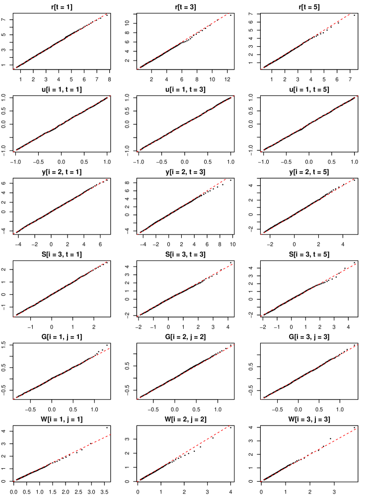
Figure 7: Comparing quantiles of the marginal-conditional draws (horizontal axis) and successive-conditional draws (vertical axis) for various elements of $(\mathbf{u}_{1:T},\,r_{1:T},\,\mathbf{s}_{1:T},\,\boldsymbol{\theta})$. If the quantiles agree, this provides evidence that the two samplers generate draws from the same distribution, which should be the case if our MCMC algorithm is error-free.

Appendix C Simulation: parameter recovery

Appendix B checked Algorithm 1 in the case of $n=2$ and $\boldsymbol{\Sigma}=\mathbf{I}_{n}$. For a cruder check that encompasses the general case and also evaluates the statistical self-consistency of the PDLM, we perform a parameter recovery exercise. We set the following:

• $n=3$; $p=n$; each $\mathbf{F}_{t}$ filled with iid draws from $\text{N}(0,\,1)$;

• $\text{vec}(\mathbf{G}^{(\text{true})})\sim\text{N}^{\star}_{p^{2}}\left(\text{vec}(0.5\cdot\mathbf{I}_{p}),\,\mathbf{I}_{p^{2}}\right)$; $\boldsymbol{\Gamma}^{(\text{true})}\sim\text{IW}_{n-1}(n+1,\,\mathbf{I}_{n-1})$; $\boldsymbol{\gamma}^{(\text{true})}\sim\text{N}_{n-1}(\mathbf{0},\,\mathbf{I}_{n-1})$; $\mathbf{W}^{(\text{true})}\sim\text{IW}_{p}(p+2,\,\mathbf{I}_{p})$;

• $\bar{\mathbf{s}}_{1|0}=\mathbf{0}$; $\mathbf{P}_{1|0}=\mathbf{I}_{p}$; $\nu_{0}=p+2$; $\boldsymbol{\Psi}_{0}=\mathbf{I}_{p}$; $\overline{\mathbf{G}}_{0}=\mathbf{0}$; $\boldsymbol{\Omega}^{-1}_{0}=\mathbf{I}_{p}$; $d_{0}=n+1$; $\boldsymbol{\Phi}_{0}=\mathbf{I}_{n-1}$; $\bar{\boldsymbol{\gamma}}_{0}=\mathbf{0}$; $\boldsymbol{\Lambda}_{0}\mathbf{I}_{n-1}$.

Based on the randomly-generated ground truth parameter values, we simulate a long time series of length $T=3200$ from the model. We recursively refit the model on an expanding window of this synthetic data, and observe in Figure 8 that the posterior distribution (visualized using boxplots of the MCMC draws) concentrates around the ground truth values (red lines) as the sample size grows.

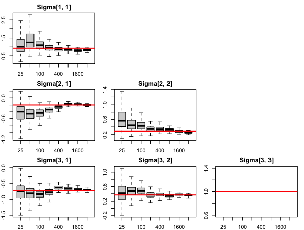
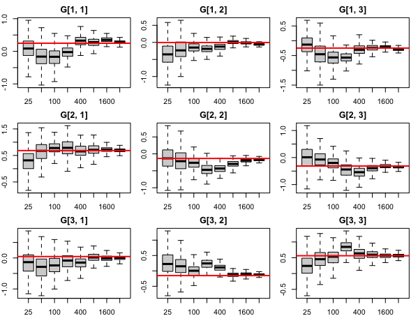
Figure 8: As we fit the PDLM to more and more simulated data, the posterior concentrates around the ground truth values for the static model parameters $\boldsymbol{\Sigma}$ and $\mathbf{G}$.

References

• Ailliot etย al. (2015) Ailliot, P., J.ย Bessac, V.ย Monbet, and F.ย Pรจne (2015): โ€œNon-homogeneous hidden Markov-switching models for wind time series,โ€ Journal of Statistical Inference and Planning, 160, 75โ€“88.
• Albert and Chib (1993) Albert, J. and S.ย Chib (1993): โ€œBayesian analysis of binary and polychotomous response data,โ€ Journal of the American Statistical Association, 88, 669โ€“679.
• Breckling (1989) Breckling, J. (1989): The Analysis of Directional Time Series: Applications to Wind Speed and Direction, Lecture Notes in Statistics, Springer.
• Carpenter etย al. (2017) Carpenter, B., A.ย Gelman, M.ย Hoffman, D.ย Lee, B.ย Goodrich, M.ย Betancourt, M.ย Brubaker, J.ย Guo, P.ย Li, and A.ย Riddell (2017): โ€œStan: a probabilistic programming language,โ€ Journal of Statistical Software, 76, 1โ€“32.
• Chan and Jeliazkov (2009) Chan, J. and I.ย Jeliazkov (2009): โ€œEfficient simulation and integrated likelihood estimation in state space models,โ€ International Journal of Mathematical Modelling and Numerical Optimisation, 1, 101โ€“120.
• Chopin (2004) Chopin, N. (2004): โ€œCentral limit theorem for sequential Monte Carlo methods and its application to Bayesian inference,โ€ Annals of Statistics, 32, 2385โ€“2411.
• Coles (1998) Coles, S. (1998): โ€œInference for circular distributions and processes,โ€ Statistics and Computing, 8, 105โ€“113.
• Craig (1988) Craig, P. (1988): โ€œTime series analysis for directional data,โ€ Ph.D. thesis, Trinity College Dublin.
• Diebolt and Robert (1994) Diebolt, J. and C.ย Robert (1994): โ€œEstimation of finite mixture distributions through Bayesian sampling,โ€ Journal of the Royal Statistical Society, Series B, 56, 363โ€“375.
• Doucet etย al. (2000) Doucet, A., N.ย de Freitas, K.ย Murphy, and S.ย Russell (2000): โ€œRao-Blackwellised particle filtering for dynamic Bayesian networks,โ€ in Proceedings of the Sixteenth Conference on Uncertainty in Artificial Intelligence, 176โ€“183.
• Doucet and Johansen (2011) Doucet, A. and A.ย Johansen (2011): โ€œA tutorial on particle filtering and smoothing: fifteen years later,โ€ in The Oxford Handbook of Nonlinear Filtering, ed. by D.ย Crisan and B.ย Rozovskiว, Oxford University Press.
• Durbin and Koopman (2002) Durbin, J. and S.ย J. Koopman (2002): โ€œA simple and efficient simulation smoother for state space time series analysis,โ€ Biometrika, 89, 603โ€“616.
• Fisher (1993) Fisher, N.ย I. (1993): Statistical Analysis of Circular Data, Cambridge.
• Fisher and Lee (1994) Fisher, N.ย I. and A.ย J. Lee (1994): โ€œTime series analysis of circular data,โ€ Journal of the Royal Statistical Society, Series B, 56, 327โ€“339.
• Garcรญa-Portuguรฉs etย al. (2014) Garcรญa-Portuguรฉs, E., A.ย Barros, R.ย Crujeiras, W.ย Gonzรกlez-Manteiga, and J.ย Pereira (2014): โ€œA test for directional-linear independence, with applications to wildfire orientation and size,โ€ Stochastic Environmental Research and Risk Assessment, 28, 1261โ€“1275.
• Garcรญa-Portuguรฉs etย al. (2013) Garcรญa-Portuguรฉs, E., R.ย Crujeiras, and W.ย Gonzรกlez-Manteiga (2013): โ€œExploring wind direction and SO2 concentration by circularโ€“linear density estimation,โ€ Stochastic Environmental Research and Risk Assessment, 27, 1055โ€“1067.
• Geweke (2004) Geweke, J. (2004): โ€œGetting it right: joint distribution tests of posterior simulators,โ€ Journal of the American Statistical Association, 99, 799โ€“804.
• Grimit etย al. (2006) Grimit, E.ย P., T.ย Gneiting, V.ย J. Berrocal, and N.ย A. Johnson (2006): โ€œThe continuous ranked probability score for circular variables and its application to mesoscale forecast ensemble verification,โ€ Quarterly Journal of the Royal Meteorological Society, 132, 2925โ€“2942.
• Harvey and Palumbo (2023) Harvey, A. and D.ย Palumbo (2023): โ€œRegime switching models for circular and linear time series,โ€ Journal of Time Series Analysis, 44, 374โ€“392.
• Hernandez-Stumpfhauser etย al. (2017) Hernandez-Stumpfhauser, D., F.ย J. Breidt, and M.ย J. van der Woerd (2017): โ€œThe general projected normal distribution of arbitrary dimension: modeling and Bayesian inference,โ€ Bayesian Analysis, 12, 113โ€“133.
• Holzmann etย al. (2006) Holzmann, H., A.ย Munk, M.ย Suster, and W.ย Zucchini (2006): โ€œHidden Markov models for circular and linear-circular time series,โ€ Environmental and Ecological Statistics, 13, 325โ€“347.
• Jona Lasinio etย al. (2020) Jona Lasinio, G., M.ย Santoro, and G.ย Mastrantonio (2020): โ€œCircSpaceTime: an R package for spatial and spatio-temporal modelling of circular data,โ€ Journal of Statistical Computation and Simulation, 90, 1315โ€“1345.
• Kantas etย al. (2015) Kantas, N., A.ย Doucet, S.ย Singh, J.ย Maciejowski, and N.ย Chopin (2015): โ€œOn particle methods for parameter estimation in state-space models,โ€ Statistical Science, 30, 328โ€“351.
• Karlsson (2013) Karlsson, S. (2013): โ€œForecasting with Bayesian vector autoregression,โ€ in Handbook of Economic Forecasting, ed. by G.ย Elliott and A.ย Timmermann, North Holland, vol.ย 2B, chap.ย 15, 791โ€“897.
• Koop (2003) Koop, G. (2003): Bayesian Econometrics, Wiley.
• Kurz etย al. (2016a) Kurz, G., I.ย Gilitschenski, and U.ย Hanebeck (2016a): โ€œRecursive Bayesian filtering in circular state spaces,โ€ IEEE Aerospace and Electronic Systems Magazine, 31, 70โ€“87.
• Kurz etย al. (2016b) โ€”โ€”โ€” (2016b): โ€œUnscented von Misesโ€“Fisher filtering,โ€ IEEE Signal Processing Letters, 23, 463โ€“467.
• Kurz etย al. (2019) Kurz, G., I.ย Gilitschenski, F.ย Pfaff, L.ย Drude, U.ย Hanebeck, R.ย Haeb-Umbach, and R.ย Siegwart (2019): โ€œDirectional statistics and filtering using libDirectional,โ€ Journal of Statistical Software, 89, 1โ€“31.
• Nuรฑez-Antonio and Gutiรฉrrez-Peรฑa (2005) Nuรฑez-Antonio, G. and E.ย Gutiรฉrrez-Peรฑa (2005): โ€œA Bayesian analysis of directional data using the projected normal distribution,โ€ Journal of Applied Statistics, 32, 995โ€“1001.
• Nuรฑez-Antonio etย al. (2011) Nuรฑez-Antonio, G., E.ย Gutiรฉrrez-Peรฑa, and G.ย Escarela (2011): โ€œA Bayesian regression model for circular data based on the projected normal distribution,โ€ Statistical Modeling, 11, 185โ€“201.
• Pewsey and Garcรญa-Portuguรฉs (2021) Pewsey, A. and E.ย Garcรญa-Portuguรฉs (2021): โ€œRecent advances in directional statistics,โ€ TEST, 30, 1โ€“58.
• Presnell etย al. (1998) Presnell, B., S.ย Morrison, and R.ย Littell (1998): โ€œProjected multivariate linear models for directional data,โ€ Journal of the American Statistical Association, 93, 1068โ€“1077.
• Robert and Roberts (2021) Robert, C. and G.ย Roberts (2021): โ€œRaoโ€“Blackwellisation in the Markov chain Monte Carlo era,โ€ International Statistical Review, 89, 237โ€“249.
• Scealy and Welsh (2011) Scealy, J.ย L. and A.ย H. Welsh (2011): โ€œRegression for compositional data by using distributions defined on the hypersphere,โ€ Journal of the Royal Statistical Society, Series B, 73, 351โ€“375.
• Wang and Gelfand (2013) Wang, F. and A.ย E. Gelfand (2013): โ€œDirectional data analysis under the general projected normal distribution,โ€ Statistical Methodology, 10, 113โ€“127.
• Zhu and Mรผller (forthcoming) Zhu, C. and H.-G. Mรผller (forthcoming): โ€œSpherical autoregressive models, with application to distributional and compositional time series,โ€ Journal of Econometrics.