Stochastic Motion Planning as Gaussian Variational Inference: Theory and Algorithms

Abstract

We consider the motion planning problem under uncertainty and address it using probabilistic inference. A collision-free motion plan with linear stochastic dynamics is modeled by a posterior distribution. Gaussian variational inference is an optimization over the path distributions to infer this posterior within the scope of Gaussian distributions. We propose Gaussian Variational Inference Motion Planner (GVI-MP) algorithm to solve this Gaussian inference, where a natural gradient paradigm is used to iteratively update the Gaussian distribution, and the factorized structure of the joint distribution is leveraged. We show that the direct optimization over the state distributions in GVI-MP is equivalent to solving a stochastic control that has a closed-form solution. Starting from this observation, we propose our second algorithm, Proximal Gradient Covariance Steering Motion Planner (PGCS-MP), to solve the same inference problem in its stochastic control form with terminal constraints. We use a proximal gradient paradigm to solve the linear stochastic control with nonlinear collision cost, where the nonlinear cost is iteratively approximated using quadratic functions and a closed-form solution can be obtained by solving a linear covariance steering at each iteration. We evaluate the effectiveness and the performance of the proposed approaches through extensive experiments on various robot models. The code for this paper can be found in https://github.com/hzyu17/VIMP.

I Introduction

Motion planning is a fundamental task for robotics systems. Robot motion planning solves the problem of navigating safely from a starting point to a target one in the state space. Path planning is a popular set of methods that was investigated in the study of the planning problem. Sampling-based techniques like Rapidly-exploring Random Trees (RRT) [1] and Probabilistic Road Map (PRM) [2] have emerged as powerful tools, constructing paths in the form of trees or graphs that facilitate the seek of optimal solutions through efficient search queries. While sampling-based approaches provide probabilistically complete solutions, a prominent drawback is their tendency to overlook the underlying dynamic characteristics of the system. Additionally, the selection of the underlying tree or graph structure can impose constraints on computational scalability. Navigating these intricacies, trajectory optimization [3, 4, 5, 6, 7] emerges as an alternative paradigm, generating sub-optimal trajectories through a constrained optimization formulation. Direct or collocation methods [3, 4, 6, 7] optimize over control and trajectory spaces, while indirect methods [8] focus exclusively on optimizing control inputs and subsequently rolling out the state trajectory for constraint validations.

Although deterministic robot motion planning is a well-studied problem [1] [5], motion planning for robots [9] in the presence of uncertainties remains a challenging task. Scenarios such as UAVs navigating turbulent airstreams [10, 11], legged robots traversing unknown terrains [12], and manipulators grasping with sensor-induced noise [13] underscore the indispensability of motion planning techniques that accommodate dynamic and environmental uncertainties. Within the trajectory optimization paradigm, robust and safe motion planning [10] [11][14] [15] models uncertainties explicitly as random processes on top of the system dynamics, and seeks robust motion plans against these uncertainties by minimizing a risk metric over the trajectory distribution. Instead of a deterministic trajectory, a tube or a funnel [11] of trajectories becomes the main pursuit. Additionally, for uncertainties in state observations, belief space motion planning [16, 17] offers an elegant framework accommodating stochastic or partially observed states.

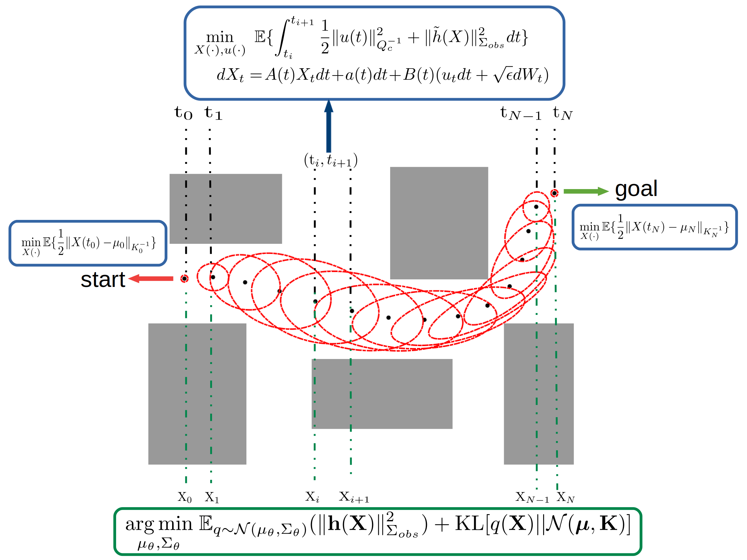
Figure 1: A visualization of the connection between Gaussian variational inference motion planning (GVI-MP) and stochastic optimal control problem over the same time discretization in a 2 dimensional robot planning example.

This study is built on the recent research by Mukadam et al. [6, 7], wherein a planning-as-inference framework was introduced, accompanied by the Maximum-a-Posteriori Motion Planning (MAP-MP) algorithm referred to as GPMP. This prior work adopted a linear Gauss-Markov process to model robot dynamics, leveraging solely the deterministic mean trajectory for feedback reference within GPMP. Building upon these foundations, our present work advances by comprehensively addressing uncertainties within linear Gauss-Markov processes, incorporating the reference trajectory distribution as a fundamental component. The trajectory perturbed by noise encapsulates uncertainties inherent in practical scenarios, encompassing imperfections in modeling and distortion of control signals. Our approach casts motion planning problems within the domain of trajectory distributions, wherein resolving this distributional problem manifests as a tenet of variational inference [18]. As a result, we introduce the Gaussian Variational Inference Motion Planning (GVI-MP) algorithm, meticulously designed to address this planning-as-inference paradigm. GVI-MP undertakes an optimization procedure within the family of Gaussian trajectory distributions, inherently yielding a trajectory ‘tube’ characterized by covariances. We show that GVI-MP gives an entropy-regularized motion plan which is robust against uncertainties in a probabilistic sense.

In the Gaussian Variational Inference Motion Planning paradigm delineated above, the optimization process directly employs the robot states as its variables. This deviates from conventional motion planning formulations, where optimization variables invariably include control inputs. To establish a coherent bridge between these two approaches, we embark on an exploration of the planning-as-inference formulation from a control-theoretic standpoint. Our investigation reveals that the Maximum-a-Posteriori (MAP) solution is equivalent to a discretization of an optimal tracking problem, whereas the Gaussian Variational Inference (GVI) solution precisely corresponds to a discretization of a stochastic control formulation featuring a terminal cost. Exploiting this intricate connection between inference and control, we revisit the planning-as-inference problem through the lens of stochastic control theory. Notably, the GVI objective aligns seamlessly with a stochastic control problem featuring boundary penalties, incorporating a non-linear collision-related state cost. Although iterative methodologies [19] have been tailored for solving nonlinear stochastic control problems with terminal costs, our formulation diverges in that the terminal cost effectively functions as a flexible constraint on boundary conditions.

A more challenging constrained linear stochastic control problem with linear dynamics and quadratic state cost was recently studied in [20] [21][22]. Termed as ‘linear covariance steering’ this novel problem diverges from conventional stochastic control paradigms by introducing a final-time constraint in lieu of a terminal cost. The domain of linear covariance steering yields an elegant, analytically tractable solution through the simultaneous solution of two interconnected Riccati equations, unified by their final-time constraints. In our investigation, we retain the linear nature of the dynamics while introducing nonlinearity via an obstacle-associated state cost. In response, we propose the Proximal Gradient Covariance Steering Motion Planning (PGCS-MP) algorithm, tailored to navigate the complexities inherent in this sophisticated nonlinear covariance steering scenario. Embedded within the iLQG lineage, PGCS-MP employs iterative proximal gradient methodology, as elaborated in [23] which is dedicated for more general nonlinear control-affine dynamics. By systematically framing each step as a linear covariance steering problem, the algorithm fuses optimization and steering paradigms in pursuit of analytical solutions.

This paper is organized as follows: Section II introduces the works that are most related to our work and summarizes the contributions of the present work. Section III introduces necessary background knowledge. Section IV presents the Gaussian Variational Inference Motion Planning theory and algorithm. Section V starts from the stochastic control perspective on GVI-MP and proposes a proximal gradient covariance steering motion planning (PGCS-MP) algorithm. Section VI presents key experimental findings, followed by the conclusion in Section VII.

II Related works and statement of contributions

We introduce the works that are most relevant to this work and then summarize our contributions.

II-A Related works

Variational inference (VI) [18] offers a solution for approximating intractable posterior distributions in Bayesian inference. VI has been widely applied to high-dimensional models and diverse machine learning contexts. In robotics, VI finds utility in robot skill learning [24], robot control and planning [25], and robot estimation tasks [26]. We use VI to address the planning-as-inference problem concerning a Gaussian path distribution. Differing from prior approaches, we incorporate the natural gradient scheme, coupling it with closed-form solutions for the Gaussian trajectory prior which are indispensable for high-DOF robot planning tasks.

GVI-MP equates to maximum-entropy stochastic motion planning through a direct objective transformation. Maximum-entropy principles, explored in reinforcement learning [27, 28] to enhance exploration and robustness in stochastic policy search, find an analogue in our work. Via the introduction of an adjustable temperature hyperparameter, our experimental findings showcase the capacity to regulate entropy levels, rendering it a discerning metric for motion plan selection.

PGCS-MP is the second algorithm that we propose to solve the planning-as-inference problem casted a stochastic control problem. Chance-constrained formulation [29] [30] [31] is one formulation in stochastic motion planning where trajectory safety is ensured via constraining the probability of collision to be less than a certain level. Chance-constrained programming involves sequential convex programming. Different from the existing work on chance-constraint formulation, we solve a covariance steering problem with nonlinear state cost using a proximal gradient paradigm. This formulation offers computationally advantageous closed-form solutions, circumventing the need for convex programs in each iteration. Such efficiency gains hold particular appeal for computation-constrained platforms and methods demanding heightened efficiency, such as model predictive control (MPC) [32][33][34].

II-B Contributions

This work investigates motion planning under uncertainties using the planning-as-inference framework. We propose two algorithms for probabilistic inference-based motion planning under uncertainty. GVI-MP employs Gaussian variational inference, optimizing discrete state variables through natural gradient descent. Meanwhile, PGCS-MP leverages proximal gradient methods to address the nonlinear covariance steering problem within the GVI-MP context. Our contributions are summarized as follows:

1. We establish theoretical connections between variational inference motion planning and stochastic control-based formulations. We show that the MAP solution discretizes linear optimal tracking, and the GVI solution encapsulates a discretization of stochastic control applicable to linear Gauss Markov systems.

2. We introduce the Gaussian Variational Inference Motion Planning (GVI-MP) algorithm for probabilistic inference-based motion planning. Additionally, we propose the Proximal Gradient Covariance Steering (PGCS-MP) algorithm, designed to solve the equivalent stochastic control problem featuring a terminal constraint.

3. We validate the efficacy of our methods via comprehensive numerical experiments, conducting analysis on the proposed methods and comparisons against baseline methods.

This work expands upon our previous contributions in [35], augmenting both theory and algorithmic dimensions of Gaussian Variational Inference Motion Planning. Theoretically, we illuminate critical insights into diverse methods for tackling planning-as-inference challenges and establish the equivalence between GPMP [7] and GVI-MP. On the algorithmic front, we provide comprehensive elaboration on GVI-MP, capitalizing on problem structure to enhance scalability. Furthermore, commencing from an equivalent stochastic control formulation, we introduce a novel algorithm, PGCS-MP, devised to solve the continuous-time nonlinear covariance steering problem.

III Background

In this section, we introduce the necessary background for our methods, including probabilistic inference motion planning, trajectory probability measure induced by stochastic dynamics, and the covariance steering problem.

III-A Probabilistic inference motion planning

Trajectory optimization leverages optimal control theory and formulates motion planning problems as an optimization

$$\begin{split}&\min_{X_{\cdot}U_{\cdot}}f_{0}(X,U)\\ &\;\;{\rm s.t.}\;\;g_{i}(X,U)\leq 0,\;i=1,\dots,m\\ &\;\;\;\;\;\;\;\;h_{i}(X,U)=0,\;i=1,\dots,r,\end{split}$$ (1)

where $f_{0}$ is the cost function and $g_{i}$’s, $h_{i}$’s are inequality and equality constraints respectively, which describe the constraints the motion planning problem is subject to. These constraints promote the feasibility of the planned trajectories for a given system and environment. The optimization is over the trajectory $X_{\cdot}$ and control input $U_{\cdot}$ jointly.

Gaussian Process Motion Planning (GPMP) [6][7] framework reformulates motion planning (1) as a probabilistic inference. The feasible plan given an environment (such as obstacles sets) is modeled as a posterior probability

$$p(\mathbf{X}|Z)\propto p(\mathbf{X})p(Z|\mathbf{X}),$$

where $\mathbf{X}$ represents a discrete trajectory, and $Z$ encodes the environment. We use the bold symbol $\mathbf{X}$ to emphasize the discrete support state representing the trajectory, which is the optimization variable in GVI-MP. The prior $p(\mathbf{X})$ represents the probability of satisfying the underlying dynamics, and likelihood $p(Z|\mathbf{X})$ encodes the probability of satisfying constraints on interacting with the environment, e.g., collision avoidance. [7] proposed a maximum-a-posterior (MAP) algorithm to find the optimal trajectory $\mathbf{X}^{\star}$ which solves

$$\mathbf{X}^{\star}=\underset{\mathbf{X}}{\arg\max}\;p(\mathbf{X}|Z)=\underset{\mathbf{X}}{\arg\max}\;p(Z|\mathbf{X})p(\mathbf{X}).$$

Diverging from the MAP trajectory approach, variational inference (VI) offers an alternative method for inferring the posterior probability $p(\mathbf{X}|Z)$ [18]. Contrasting the quest for a deterministic solution $\mathbf{X}^{\star}$, VI aims to minimize the divergence between a proposed distribution and $p(\mathbf{X}|Z)$. Gaussian Variational Inference (GVI), a specific instance of VI, confines the optimization within Gaussian distribution. In this study, we account for additive noise within the control channel, capturing deviations from an ideal execution in lower-level controllers [33]. Once the control input is translated through controlled dynamics into the state space, stochasticity manifests within the states as well.

III-B Trajectory distribution and Girsanov theorem

Now we introduce the notion of path distribution induced by stochastic differential equation (SDE), and Girsanov theorem [36]. Girsanov theorem is an important theorem in stochastic calculus, which is often used to transform the probability measures of SDEs. Consider first the SDE

$$dX_{t}=f(X_{t},t)dt+dW_{t}$$

where $X_{t}$ is the state, and $W_{t}$ is a standard Wiener process This SDE induces a probability space over the trajectories where every single trajectory is one sample from this distribution. Denote the probability density of path $X_{t}$ as $d{\mathbb{P}}\triangleq p(X_{t})$. Given two SDEs with the same initial conditions

$$dX_{t}=f_{1}(X_{t},t)dt+dW_{t},$$ (2)

and

$$dY_{t}=f_{2}(Y_{t},t)dt+dW_{t},$$ (3)

Girsanov states that the probability density ratio between the two paths is given by [36]

$$\frac{d{\mathbb{P}}_{X}}{d{\mathbb{P}}_{Y}}=Z(t),$$

where

$$Z(t) =\exp(-\frac{1}{2}\int_{0}^{t}[f_{1}(X_{\tau})-f_{2}(Y_{\tau})]^{T}[f_{1}(X_{\tau})-f_{2}(Y_{\tau})]d\tau$$

$$\hskip 31.2982pt+\int_{0}^{t}[f_{1}(X_{\tau})-f_{2}(Y_{\tau})]^{T}dW_{t}).$$

Denote continuous paths generated by (2) and (3) as $\mathcal{X}(t),\mathcal{Y}(t)$ respectively, i.e.,

$$\mathcal{X}(t)=\{X_{\tau}|0\leq\tau\leq t\},\;\;\mathcal{Y}(t)=\{Y_{\tau}|0\leq\tau\leq t\},$$

then for an arbitrary function $w(\cdot)$ of the path from $0$ to $t$, the expectation over the randomness induced by the Brownian motion has the relation

$${\mathbb{E}}[w(\mathcal{X}(t))]={\mathbb{E}}[Z(t)w(\mathcal{Y}(t))].$$

III-C Linear covariance steering

The linear covariance steering problem is presented in the following form [21]

$$\min_{u} {\mathbb{E}}\left\{\int_{0}^{T}[\frac{1}{2}\|u_{t}\|^{2}+\frac{1}{2}X_{t}^{T}Q_{t}X_{t}]dt\right\}$$ (4c)

$$dX_{t}=A_{t}X_{t}dt+a_{t}dt+B_{t}(u_{t}dt+\sqrt{\epsilon}dW_{t})$$

$$X_{0}\sim\mathcal{N}(\mu_{0},K_{0}),\quad X_{T}\sim\mathcal{N}(\mu_{T},K_{T}).$$

The dynamics is linear, the costs include a minimum control energy and a quadratic state cost, and the initial and final time boundaries are all Gaussian distributions. The optimal solution to (4) is obtained by controlling the mean and the covariance separately thanks to the linearity. The control for the mean is a classical optimal control problem

$$\min_{v} \int_{0}^{T}[\frac{1}{2}\|v_{t}\|^{2}+\frac{1}{2}x_{t}^{T}Q_{t}x_{t}]dt$$

$$\dot{x}_{t}=A_{t}x_{t}+B_{t}v_{t}$$

$$x_{0}=\mu_{0},\quad x_{T}=\mu_{T}.$$

The optimal control of the covariance is obtained by solving the coupled Riccati equations [22]

$$-\dot{\Pi}_{t}\!\!\!\! = \!\!\!\!A_{t}^{T}\Pi_{t}\!+\!\Pi_{t}A_{t}\!-\!\Pi_{t}B_{t}B_{t}^{T}\Pi_{t}\!+\!Q_{t}$$ (6a)

$$-\dot{\mathrm{H}}_{t}\!\!\!\! = \!\!\!\!A_{t}^{T}{\mathrm{H}}_{t}\!+\!{\mathrm{H}}_{t}A_{t}\!+\!{\mathrm{H}}_{t}B_{t}B_{t}^{T}{\mathrm{H}}_{t}\!-\!Q_{t}$$ (6b)

$$\epsilon K_{0}^{-1}\!\!\!\! = \!\!\!\!\Pi_{0}+{\mathrm{H}}_{0}$$ (6c)

$$\epsilon K_{T}^{-1}\!\!\!\! = \!\!\!\!\Pi_{T}+{\mathrm{H}}_{T}.$$ (6d)

The coupled Ricatti equation system has a closed-form solution. We refer to [20] for details. Denote the optimal control for mean to be $v_{t}^{\star}$ and corresponding state trajectory to be $x_{t}^{\star}$. Combining it with the covariance control yields the optimal feedback policy

$$u_{t}^{\star}=-B_{t}^{T}\Pi(t)(X_{t}-x_{t}^{\star})+v_{t}^{\star}.$$

IV Gaussian variational inference motion planning (GVI-MP)

In this section we introduce the probabilistic inference motion planning and propose the GVI-MP algorithm.

IV-A Gaussian process motion planning (GPMP)

a) Gaussian trajectory prior. GPMP [6] [7] reformulates the trajectory optimization problem into probabilistic inference. We make the same assumption that robot trajectories are sampled from a parameterized Gaussian process (GP) $X_{t}\sim\mathcal{GP}(\mu(t),\mathcal{K}(t,t^{\prime}))$. $\mathcal{GP}$ defines a continuous trajectory prior. We consider a time-varying linear Gauss-Markov model with known initial distribution [37, 7]

$$dX_{t}=A_{t}X_{t}dt+a_{t}dt+B_{t}dW_{t},\;\;X_{0}\sim\mathcal{N}(\mu_{0},K_{0})$$ (7)

to represent the underlying dynamics that generate the GP kernel. The solution to (7) is

$$X_{t}=\Phi(t,0)X_{0}+\int_{0}^{t}\Phi(t,s)a_{s}ds+\int_{0}^{t}\Phi(t,s)B_{s}dW_{s},$$ (8)

where $\Phi(t,s)$ is the state transition kernel. The mean and covariance of the GP are

$$\mu(t) = \Phi(t,0)\mu_{0}+\int_{0}^{t}\Phi(t,s)a_{s}ds,$$

$$K(t,t^{\prime}) = \Phi(t,0)K_{0}\Phi(t^{\prime},0)^{T}+$$

$$\int_{0}^{{\rm min}(t,t^{\prime})}\Phi(t,s)B_{s}B_{s}^{T}\Phi(t^{\prime},s)^{T}ds.$$

We represent robot trajectory using support states $\mathbf{X}$ over a time discretization $\mathbf{t}=[t_{0},\dots,t_{N}].$ We let $t_{0}=0$ and $t_{N}=T$ to make the discretization consistent with continuous-time formulations. For a Gaussian process, the discrete joint trajectory distribution over $\mathbf{t}$ is a Gaussian distribution

$$\tilde{p}(\mathbf{X})\triangleq p(X_{0})p(X_{1}|X_{0}),\dots,p(X_{N}|X_{N-1}).$$

A terminal condition at $t_{N}$ can be imposed by conditioning $\tilde{p}(\mathbf{X})$ on a fictitious observation $O_{t_{N}}\sim\mathcal{N}(\mu_{N},K_{N})$, leading to a conditional Gaussian

$$p(\mathbf{X})=\tilde{p}(\mathbf{X}|O_{t_{N}})\propto\exp(-\frac{1}{2}(\lVert\mathbf{X}-{\boldsymbol{\mu}}\rVert_{\mathbf{K}^{-1}}^{2})).$$ (9)

We term (9) the trajectory prior [7]. In the special case or linear Gauss-Markov process (7), the support means ${\boldsymbol{\mu}}=[\mu_{0},\dots,\mu_{N}]$ where

$$\mu_{i}=\Phi(t,t_{0})\mu_{0}+\int_{t_{0}}^{t_{i}}\Phi(t_{i},s)a_{s}ds,$$

and the joint precision matrix $\mathbf{K}^{-1}=G^{T}Q^{-1}G$ has a known sparsity pattern [37]

$$G=\begin{bmatrix}I&&&&\\ -\Phi(t_{1},t_{0})&I&&&\\ &&\dots&&\\ &&&-\Phi(t_{N},t_{N-1})&I\\ &&&0&I\end{bmatrix},$$ (10)

and

$$Q^{-1}={\rm diag}(K_{0}^{-1},Q_{0,1}^{-1},\ldots,Q_{N-1,N}^{-1},K_{N}^{-1}).$$ (11)

Here $Q_{i,i+1}$ is a Grammian

$$Q_{i,i+1}=\int_{t_{i}}^{t_{i+1}}\Phi(t_{i+1},s)B_{s}B_{s}^{T}\Phi(t_{i+1},s)^{T}ds,$$ (12)

and $K_{0},K_{N}$ are desired start and goal states covariances.

b) Collision avoidance likelihood. The likelihood factor is defined by collision costs

$$p(Z|\mathbf{X})\propto\exp(-\lVert\tilde{\mathbf{h}}(S(F(\mathbf{X})))\rVert_{\Sigma_{\rm obs}}^{2}),$$ (13)

where $\tilde{\mathbf{h}}(\cdot)$ is a hinge loss function, $S(\cdot)$ is the signed distance to the obstacles, $F(\cdot)$ represents the robot’s forward kinematics, and $\Sigma_{obs}$ is a weight applied on the hinge losses. For notation simplicity, we denote hereafter the composite loss function by

$$\mathbf{h}(\mathbf{X})=\tilde{\mathbf{h}}(S(F(\mathbf{X}))).$$ (14)

We emphasize by using bold symbols that the hinge loss $\tilde{\mathbf{h}}$ is a vector which can represent multiple collision checking points on a robot. Combining the prior $p(\mathbf{X})$ defined in (9) and the likelihood $p(Z|\mathbf{X})$ in (13), the MAP formulation (III-A) can be written explicitly as

$$\begin{split}\mathbf{X}^{\star}&=\underset{\mathbf{X}}{\arg\max}\;p(Z|\mathbf{X})p(\mathbf{X})\\ &=\underset{\mathbf{X}}{\arg\min}\;\lVert\mathbf{h}(\mathbf{X})\rVert_{\Sigma_{\rm obs}}^{2}+\frac{1}{2}\lVert\mathbf{X}-{\boldsymbol{\mu}}\rVert_{\mathbf{K}^{-1}}^{2}\end{split}$$ (15)

IV-B Gaussian variational inference motion planning (GVI-MP)

a) Objectives. The probabilistic inference formulation provides an alternative view on motion planning, which opens the door for methods for solving inference problems to find their applications in solving motion planning problems. Solving the MAP problem (15) [38] [7] gives deterministic solutions. In contrast, our GVI-MP formulation is written as

$$\begin{split}q^{\star}&=\underset{q\in\mathcal{Q}}{\arg\min}\;{\rm KL}[q(\mathbf{X})||p(\mathbf{X}|Z)]\\ &=\underset{q\in\mathcal{Q}}{\arg\min}\;{\mathbb{E}}_{q}{[\log q(\mathbf{X})-\log p(Z|\mathbf{X})-\log p(\mathbf{X})]}\\ &=\underset{q\in\mathcal{Q}}{\arg\max}\;{\mathbb{E}}_{q}{\log p(Z|\mathbf{X})}-{\rm KL}[q(\mathbf{X})||p(\mathbf{X})]\\ &=\underset{\mu_{\theta},\Sigma_{\theta}}{\arg\min}\;{\mathbb{E}}_{q\sim\mathcal{N}(\mu_{\theta},\Sigma_{\theta})}{(\lVert\mathbf{h}(\mathbf{X})\rVert_{\Sigma_{\rm obs}}^{2})}+{\rm KL}[q||\mathcal{N}({\boldsymbol{\mu}},\mathbf{K})]\end{split}$$ (16)

where $\mathcal{Q}\triangleq\mathcal{N}(\mu_{\theta},\Sigma_{\theta})$ stands for the proposed parameterized Gaussian distributions. The prior $p(\mathbf{X})$ is in the form (9) with sparsity in $\mathbf{K}^{-1}$ and the likelihood is in the form (13). In the variational inference problem, we seek a joint Gaussian trajectory distribution with a minimum distance to the motion planning posterior distribution measured by KL divergence.

GVI-MP is equivalent to an entropy-regularized motion planning by rewriting equation (16)

$$\begin{split}q^{\star}&=\underset{q\in\mathcal{Q}}{\arg\min}\;{\rm KL}[q(\mathbf{X})||p(\mathbf{X}|Z)]\\ &=\underset{q\in\mathcal{Q}}{\arg\max}\;{\mathbb{E}}_{q}[\log p(\mathbf{X}|Z)]+H(q(\mathbf{X}))\\ &=\underset{q\in\mathcal{Q}}{\arg\max}\;{\mathbb{E}}_{q}[\log p(\mathbf{X})+\log p(Z|\mathbf{X})]+H(q(\mathbf{X})),\end{split}$$ (17)

wherein the objective maximizes the log probability of the posterior $p(\mathbf{X}|Z)$ in (15). In addition, it also maximizes an entropy regularization term

$$\begin{split}H(q)&=-{\mathbb{E}}_{q}\log q(\mathbf{X})\\ &\propto-{\mathbb{E}}\{\log[(\det\Sigma_{\theta})^{-\frac{1}{2}}\exp(-\frac{1}{2}(\mathbf{X}-{\boldsymbol{\mu}})\Sigma_{\theta}^{-1}(\mathbf{X}-{\boldsymbol{\mu}}))]\}\\ &\propto\log\det\Sigma_{\theta}.\end{split}$$

In the context of Gaussian distributions, $\det\Sigma_{\theta}$ scales with the equi-density contour ellipsoids’ volume $\mathcal{E}$ [39]. Maximizing $\mathcal{E}$ equates to maximizing $\log\det\Sigma_{\theta}$. Hence, maximizing entropy in motion planning entails expanding the feasible and safe trajectory distribution around the mean to encompass the highest possible space, considering a designated confidence level $\rho$. Put simply, elevated entropy widens the trajectory distribution funnel across the state space.

b) Robust motion planning.

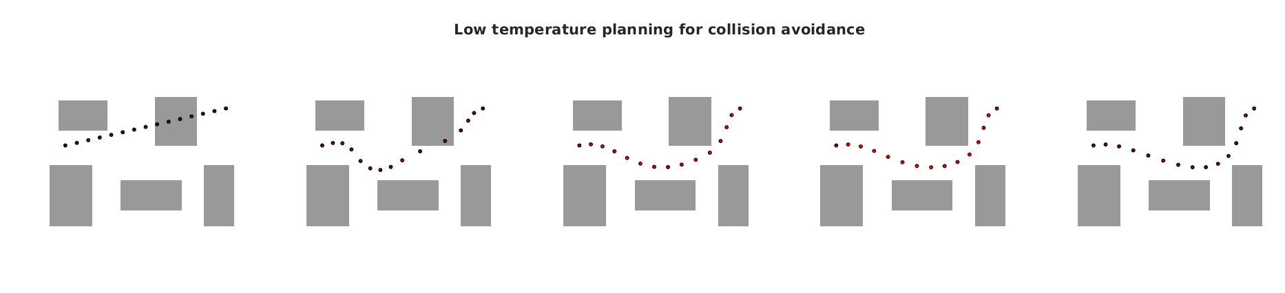
Figure 2: The low-temperature and high-temperature planning for a maximum entropy robust motion plan. In the low temperature phase, the motion planner puts more weights on feasiblility of a motion plan, i.e., the collision avoidance while enforcing the dynamics. In the high temperature phase, the planner puts more weights on robustness by maximizing the trajectory’s entropy.

We characterize the plan’s robustness against uncertainties by pursuing increased maneuvering space during planning to accommodate tracking errors in execution. The motion planning objectives find expression in the posterior probability $p(\mathbf{X}|Z)$, where the prior $p(\mathbf{X})$ enforces the dynamics prior (7) with initial and terminal marginals $\mathcal{N}(\mu_{0},K_{0})$ and $\mathcal{N}(\mu_{N},K_{N})$; the likelihood $p(Z|\mathbf{X})$ captures the collision avoidance penalty on support states. The ratio between the two encapsulates the balance between dynamics and collision-free constraints. In more complex environments, on top of collision avoidance, the safety and robustness of a plan should also be taken into consideration. Imagine a moving robot traversing a cluttered environment. There exists a trade-off between the shortest but risky path and a longer but safer path. The entropy regularization on top of the motion planning objective captures this trade-off.

To trade the weights on motion planning objectives and the entropy, we introduce a hyperparameter termed temperature $\hat{T}$ into the objective (17)

$$q^{\star}=\underset{q\in\mathcal{Q}}{\arg\max}\;{\mathbb{E}}_{q}[\log p(\mathbf{X})+\log p(Z|\mathbf{X})]+\hat{T}\,H(q(\mathbf{X})).$$

The optimization unfolds in two distinct phases—low-temperature and high-temperature. The former ensures a concise, obstacle-free plan, while the latter instills probabilistic robustness into the plan. An illustrative example is presented in Figure 3. On the left, a shortcut solution appears but is inherently riskier due to a narrow gap between obstacles. Conversely, the right-side solution entails a longer trajectory with heightened prior cost, yet its smaller entropy cost (evident in the extended covariance matrices) encapsulates enhanced visual robustness. The comparison showcases that the entropy in the planning context reflects the risk constraints of the current environment in a probabilistic sense. Table I compiles the costs for the plans depicted in Figure 3. The difference in entropy costs impacts the total cost between the left and right solutions. To elucidate, our inclusion of entropy prompts the preference for a longer yet less precarious plan over a shorter but riskier alternative.

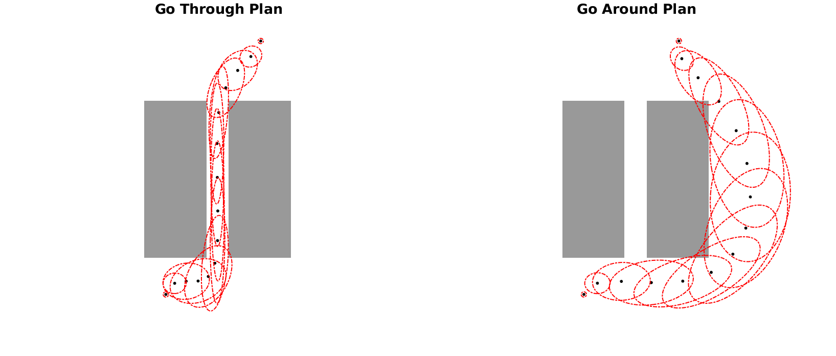
Figure 3: Entropy regularized motion planning [35].

	Prior	Collision	MP	Entropy	Total
Left	34.4583	9.1584	43.6168	44.1752	87.7920
Right	42.9730	2.0464	45.0193	39.9193	84.9387

TABLE I: Comparing costs for plans in Fig. 3. The regularized entropy cost $\log(\lvert\Sigma_{\theta}^{-1}\rvert)$ changed the order of the total costs and enables our optimization to choose a probabilistically less risky solution. ‘MP’ stands for motion planning costs which is the sum of prior and collision costs.

IV-C Optimization scheme for GVI-MP

a) Natural gradient descent. We use a natural gradient scheme to guide the candidate Gaussian towards the desired posterior. To maintain notational simplicity, we define the negative log probability for the posterior as $\psi(\mathbf{X})=-\log p(\mathbf{X}|Z)$, and the objective in (16) minimizes

$$J(q)={\rm KL}[q(\mathbf{X})||p(\mathbf{X}|Z)]=-H(q)+{\mathbb{E}}[\psi(\mathbf{X})].$$

The sparsity of the Gaussian prior leads to an exact sparse Gaussian inference problem. We parameterize the proposed Gaussian using its mean $\mu_{\theta}$ and inverse of covariance $\Sigma^{-1}_{\theta}$ [26]. The derivatives with respect to $\mu_{\theta}$ and $\Sigma^{-1}_{\theta}$ are [40]

$$\frac{\partial J(q)}{\partial\mu_{\theta}} =\Sigma^{-1}_{\theta}{\mathbb{E}}[(\mathbf{X}-\mu_{\theta})\psi]$$ (18a)

$$\frac{\partial^{2}J(q)}{\partial\mu_{\theta}\partial\mu_{\theta}^{T}} =\Sigma^{-1}_{\theta}{\mathbb{E}}[(\mathbf{X}-\!\mu_{\theta})(\mathbf{X}\!-\!\mu_{\theta})^{T}\psi]\Sigma^{-1}_{\theta}\!-\!\!\Sigma^{-1}_{\theta}{\mathbb{E}}[\psi]$$ (18b)

$$\frac{\partial J(q)}{\partial\Sigma^{-1}_{\theta}} =\frac{1}{2}\Sigma_{\theta}{\mathbb{E}}[\psi]\!-\!\frac{1}{2}{\mathbb{E}}[(\mathbf{X}-\!\mu_{\theta})(\mathbf{X}-\!\mu_{\theta})^{T}\psi]+\frac{1}{2}\Sigma_{\theta}.$$ (18c)

Comparing (18b) and (18c) we obtain

$$\frac{\partial^{2}J(q)}{\partial\mu_{\theta}\partial\mu_{\theta}^{T}}=\Sigma^{-1}_{\theta}-2\Sigma^{-1}_{\theta}\frac{\partial J(q)}{\partial\Sigma^{-1}_{\theta}}\Sigma^{-1}_{\theta},$$ (19)

which makes it unneccessary to evaluate both (18b) and (18c). Natural gradient descent update step w.r.t. objective function $J$ is standard [41]

$$\begin{bmatrix}\delta\mu_{\theta}\\ vec(\delta\Sigma^{-1}_{\theta})\end{bmatrix}=-\begin{bmatrix}\Sigma_{\theta}&0\\ 0&2(\Sigma^{-1}_{\theta}\otimes\Sigma^{-1}_{\theta})\end{bmatrix}\begin{bmatrix}\frac{\partial J(q)}{\partial\mu_{\theta}}\\ vec(\frac{\partial J(q)}{\partial\Sigma^{-1}_{\theta}})\end{bmatrix},$$

which in matrix form is written as

$$\Sigma^{-1}_{\theta}\delta\mu_{\theta}=-\frac{\partial J(q)}{\partial\mu_{\theta}},\;\;\;\delta\Sigma^{-1}_{\theta}=-2\Sigma^{-1}_{\theta}\frac{\partial J(q)}{\partial\Sigma^{-1}_{\theta}}\Sigma^{-1}_{\theta}.$$ (20)

Comparing (18) and (20), we have

$$\delta\Sigma^{-1}_{\theta} =\frac{\partial^{2}J(q)}{\partial\mu_{\theta}\partial\mu_{\theta}^{T}}-\Sigma^{-1}_{\theta}.$$ (21)

Equation (20) and (21) tells that, to calculate the update $\delta\mu_{\theta},\delta\Sigma^{-1}_{\theta}$, we only need to compute the expectations (18a) and (18b). The updates use a step size $\eta<1$

$$\mu_{\theta}\leftarrow\mu_{\theta}+\eta^{R}\,\delta\mu_{\theta},\;\;\;\Sigma^{-1}_{\theta}\leftarrow\Sigma^{-1}_{\theta}+\eta^{R}\,\delta\Sigma^{-1}_{\theta},$$ (22)

with an increasing $R>1$ to shrink the step size for backtracking until the cost decreases.

b) Sparsity and factorization. To leverage the sparsity of the information matrix $\Sigma_{\theta}^{-1}$, we factorize the objective and the variables. The log probability of the posterior $\psi(\mathbf{X})$ can be factorized due to the sparsity in matrix $\mathbf{K}^{-1}$, leading to

$$\psi(\mathbf{X})=\sum_{l=1}^{L}\psi_{\ell}(\mathbf{X})\triangleq-\log p(\mathbf{X}_{\ell}|Z),$$ (23)

where factor level marginal Gaussian variables are mapped to and from the joint variables linearly using a mapping $M_{\ell}$

$$q_{\ell}\sim\mathcal{N}(\mu_{\theta}^{\ell},\Sigma_{\theta}^{\ell}),\;\;\mu_{\theta}^{\ell}=M_{\ell}\mu_{\theta},\;\;\Sigma_{\theta}^{\ell}=M_{\ell}\Sigma_{\theta}M_{\ell}^{T}.$$ (24)

In view of (24), the gradient updates (18a) and (18b) can be evaluated on factor levels, then mapped to the joint level as

$$\begin{split}\frac{\partial J(q)}{\partial\mu_{\theta}}=\sum_{l=1}^{L}M_{\ell}^{T}\frac{\partial J_{\ell}(q_{\ell})}{\partial\mu_{\theta}^{\ell}},\frac{\partial^{2}J(q)}{\partial\mu_{\theta}\partial\mu_{\theta}^{T}}=\sum_{l=1}^{L}M_{\ell}^{T}\frac{\partial^{2}J_{\ell}(q_{\ell})}{\partial\mu_{\theta}^{l}(\partial\mu_{\theta}^{l})^{T}}M_{\ell},\end{split}$$

where $L$ is the total number of factors and $J_{\ell}(q_{\ell})\triangleq{\mathbb{E}}_{q_{\ell}}[\psi_{\ell}(\mathbf{X})]$ represents factor level objectives.

IV-D Posterior structures in motion planning inference tasks

Natural gradient descent updates necessitate computing the expectations (18) with respect to the proposed Gaussian $q$. Leveraging the log posterior’s structure, we streamline these computations. By the definition (15), we express $\psi(\mathbf{X})$ as

$$\psi(\mathbf{X})=-\log p(\mathbf{X}|Z)=\lVert\mathbf{h}(\mathbf{X})\rVert_{\Sigma_{\rm obs}}^{2}+\frac{1}{2}\lVert\mathbf{X}-{\boldsymbol{\mu}}\rVert_{\mathbf{K}^{-1}}^{2},$$

which consists of a quadratic $\psi_{\rm{Prior}}$ for the prior and a nonlinear factor $\psi_{\rm{NL}}$ for the collision checking defined as

$$\psi_{\rm{Prior}}(\mathbf{X})=\frac{1}{2}\lVert\mathbf{X}-{\boldsymbol{\mu}}\rVert_{\mathbf{K}^{-1}}^{2},\;\;\psi_{\rm{NL}}(\mathbf{X})=\lVert\mathbf{h}(\mathbf{X})\rVert_{\Sigma_{\rm obs}}^{2}.$$ (25)

a) The prior factor $\psi_{\rm Prior}$ contains a sparse precision matrix $\mathbf{K}^{-1}$ as in (10). If we denote

$$\delta X_{j}=X_{j}-\mu_{j},\;\;j=0,\dots,N,$$

then

$$\begin{split}\psi_{\rm{Prior}}(\mathbf{X})&\propto{\mathbb{E}}\{(\mathbf{X}-{\boldsymbol{\mu}})^{T}G^{T}Q^{-1}G(\mathbf{X}-{\boldsymbol{\mu}})\}\\ &={\mathbb{E}}\{\lVert[(\delta X_{0})^{T},(\delta X_{1}-\Phi_{1,0}\delta X_{0})^{T},\dots,\\ &\hskip 5.69046pt(\delta X_{N}-\Phi_{N,N-1}\delta X_{N-1})^{T},\delta X_{N}^{T}]^{T}\rVert_{Q^{-1}}^{2}\},\end{split}$$

which can be further decomposed into

$$J_{0}(q_{0})+J_{0,1}(q_{0,1})+\dots+J_{N}(q_{N})$$

by defining the factorized costs

$$\begin{split}J_{0}(q_{0})&\triangleq{\mathbb{E}}_{q_{0}}\{\lVert\delta X_{0}\rVert_{{K^{-1}_{0}}}^{2}\},\\ J_{i,i+1}(q_{i,i+1})&\triangleq{\mathbb{E}}_{q_{i,i+1}}\{\lVert\delta X_{i+1}-\Phi_{i+1,i}\delta X_{i}\rVert_{Q^{-1}_{i,i+1}}^{2}\},\\ J_{N}(q_{N})&\triangleq{\mathbb{E}}_{q_{N}}\{\lVert\delta X_{N}\rVert_{{K^{-1}_{N}}}^{2}\},\end{split}$$

where $q_{0}$ and $q_{N}$ are the marginal Gaussian distributions of the first and last supported states, and $q_{i,i+1}$ stand for marginal Gaussian distributions of consecutive two states in between.

The factors $J_{i,i+1}(q_{i,i+1})$ enforce the underlying dynamics on consecutive states while the two isolate factors $J_{0}$ and $J_{N}$ enforce the initial and terminal conditions. Notice that because of the underlying linear dynamics, both $J_{i,i+1},J_{0}$, and $J_{N}$ have quadratic functions inside the expectation. We show in the following lemma that the derivatives in (18a) and (18b) for such quadratic factors enjoy a close form.

Lemma 1.

For given matrices $\Lambda,\Psi$ with right dimensions, define $y\triangleq\mathbf{X}-\mu_{\theta}$, the derivatives of $J={\mathbb{E}}[\lVert\Lambda\mathbf{X}-\Psi{\boldsymbol{\mu}}\rVert_{\mathbf{K}^{-1}}^{2}]$ are

$$\frac{\partial J}{\partial\mu_{\theta}} =2\Lambda^{T}\mathbf{K}^{-1}(\Lambda\mu_{\theta}-\Psi{\boldsymbol{\mu}}).$$ (26a)

$$\frac{\partial^{2}J}{\partial\mu_{\theta}\partial\mu_{\theta}^{T}} =\Sigma^{-1}_{\theta}{\mathbb{E}}[yy^{T}y^{T}\Lambda^{T}\mathbf{K}^{-1}\Lambda y]\Sigma^{-1}_{\theta}$$

$$\;\;\;\;-\Sigma^{-1}_{\theta}\operatorname{Tr}[\Lambda^{T}\mathbf{K}^{-1}\Lambda\Sigma_{\theta}].$$ (26b)

Proof.

See Appendix -A. ∎

The closed-form derivatives for the motion prior can be obtained by letting

$$\Lambda=[-\Phi_{i+1,i},I],~{}\Psi=[\Phi_{i+1,i},-I]$$

for $J_{i,i+1}$, and letting $\Lambda=I,~{}\Psi=0$ for $J_{0},~{}J_{N}$, where the Gaussian variables are the corresponding marginals $q_{0},q_{i+1,i}$, and $q_{N}$, respectively. The closed-form updates on the motion priors greatly accelerates the algorithm compared with Monte Carlo estimations or quadratures. In the special case of zero drift dynamics, i.e., $a_{t}=0$ in (7), we have

$$J_{i,i+1}(q_{i,i+1})={\mathbb{E}}_{q_{i,i+1}}\{\lVert X_{i+1}-\Phi_{i+1,i}X_{i}\rVert_{Q^{-1}_{i,i+1}}^{2}\}.$$

b) The collision likelihood factors $\psi_{\rm{NL}}$ are evaluated on each support state, which forms a series of isolated factors

$$\psi_{\rm{NL}}(\mathbf{X})=\lVert\mathbf{h}(\mathbf{X})\rVert_{\Sigma_{\rm obs}}^{2}=\sum_{n=0}^{N}\lVert\mathbf{h}(X_{t_{n}})\rVert_{\Sigma_{\rm obs}}^{2}.$$ (27)

Computing expectations with respect to Gaussian distributions over nonlinear factors has been extensively explored within the Gaussian filtering literature [42, 43]. A prominent numerical technique employed for this purpose is Gauss-Hermite (GH) quadrature [44], notably employed in nonlinear filtering problems, giving rise to the Gauss-Hermite Filter (GHF) [43]. We employ GH quadratures to approximate the expected nonlinear collision avoidance factor. Details on the GH quadrature method are provided in Appendix -B.

By combining the prior (9) and the likelihood (13), we parameterize the inverse covariance $\Sigma_{\theta}^{-1}$ as a sparse matrix mirroring $\mathbf{K}^{-1}$’s sparsity. For motion planning involving $N+1$ support states, a total of $2N+3$ factors need to be computed. Among these, $N+2$ quadratic factors admit closed-form solutions, while the remaining $N+1$ nonlinear factors are evaluated via GH quadratures. Although the computations transpire at the factor level, our subsequent discourse adopts a joint level presentation for simplicity.

c) GVI-MP Algorithm.

1

input : Initial proposal $(\mu_{\theta},\Sigma_{\theta})$, stepsize $\eta$, max number of backtrack iterations $I_{b}$, temperature $\hat{T}$, number of low-temperature iterations $I_{\ell}$, high temperature $\hat{T}_{h}$ and SDF.

output : Optimized trajectory distribution ${\mathcal{N}}(\mu_{\theta}^{*},\Sigma_{\theta}^{*})$.

2 for $i=1,2,\ldots$ do

3       if $i==I_{\ell}$ then

4             Switch to high temperature and re-intialize the precision matrix variable.

5      for $r=1,2,\ldots,{\rm R}$  do

6             for $k=1,2,\dots,K$ do

7                   Map to the factorized level.

8                  Compute (18) for $\psi_{\rm Quad}$ using closed-form (26).

9                  Compute (18) for $\psi_{\rm NL}$ using G-H quadratures in appendix -B.

10            Map to the global level.

11            Compute $\delta\mu_{\theta},\delta\Sigma^{-1}_{\theta}$ using (20) and (21).

12            Backtrack $(\mu_{\theta},\Sigma_{\theta})$ using (22), until decrease in cost $J$ or reach the threshold $I_{b}$.

13      

Algorithm 1 Gaussian Variational Inference Motion Planning (GVI-MP)

The Gaussian Variational Inference Motion Planning (GVI-MP) algorithm is formalized in Algorithm 1. This entails factorized structures and a backtracking search to determine step size within the natural gradient descent framework. Algorithm 1 embodies three nested loops: the outermost loop governs natural gradient iterations, the middle loop handles backtracking search for optimal step size at each iteration, and the innermost loop computes derivatives across all factors.

V Proximal Gradient Covariance Steering Motion Planning (PGCS-MP)

GVI-MP addresses a probabilistic inference problem directly on the distribution over the discretized support states $\mathbf{X}$. However, in the context of trajectory optimization formulation (1), the optimization involves both $X_{t}$ and $U_{t}$. In the subsequent section, we aim to establish the relationship between these two formulations and explore the underlying reason for the omission of the control variable $U_{t}$.

V-A GPMP as minimum-energy feedback motion planning

The MAP formulation (15) is an optimization over the support states $\mathbf{X}$ for finding the maximum-a-posterior probability $p(\mathbf{X}|Z)$. At first sight, this problem resembles a classical path planning problem without control and dynamics. However, a deeper look into the solution tells that it is actually equivalent to a closed-form solution to a minimum-energy tracking problem with the nominal trajectory being exactly the mean trajectory of the Gauss-Markov process (7).

Lemma 2.

The optimal solution to the following problem is the MAP solution to the probabilistic inference (15) over the same time discretization

$$\min_{X(\cdot),u(\cdot)}\!\!\!\!\!\!\! \int_{t_{0}}^{t_{N}}\frac{1}{2}\|u_{t}\|^{2}+\lVert\mathbf{h}(X_{t})\rVert_{\Sigma_{\rm obs}}^{2}dt$$ (28b)

$$+\frac{1}{2}\lVert X_{0}-\mu_{0}\rVert_{K_{0}^{-1}}^{2}+\frac{1}{2}\lVert X_{N}-\mu_{N}\rVert_{K_{N}^{-1}}^{2}$$

$$\dot{\delta X_{t}}=A_{t}\delta X_{t}+a_{t}+B_{t}u_{t},$$

where $\delta X_{t}\triangleq X_{t}-\mu_{t}$ is the deviation from the nominal mean trajectory induced by the prior process (7).

Proof.

See Appendix -C. ∎

Lemma 2 analyzes the MAP formulation from a control perspective. This equivalence is due to (28) admits a closed-form feedback solution whose feedback gain is related to the same Grammian as in (11). Formulation (28) is a classical feedback motion planning [1] where a feedback control law around a nominal trajectory $\mu_{t}$ is obtained. Here the minimum control energy cost is a special case of the LQR problem with zero state cost, which has a closed-form solution instead of solving a Riccati equation within each time interval. This closed-form feedback solution maps the optimal control onto the state trajectory, resulting in an optimization only over the state trajectory as in the MAP formulation. In MAP-MP formulation, although the prior trajectory is a SDE-generated Gaussian process, the dynamics for the nominal mean trajectory and the deviated states are deterministic, where the mean trajectory $\mu_{t}$ of the prior process (7) is governed by $\dot{\mu}_{t}=A_{t}\mu_{t}+a_{t}.$ Similar to popularly used polynomials or splines, using the mean of a Gaussian process captures the smoothness of the robot trajectory and the underlying dynamics. The conditional initial and final marginal distribution of the prior in the MAP formulation (15) is enforced by boundary costs $\lVert X_{0}-\mu_{0}\rVert_{K_{0}}^{2}$ and $\lVert X_{N}-\mu_{N}\rVert_{K_{N}}^{2}$.

V-B GVI-MP as stochastic motion planning

Building upon the equivalence between the MAP solution and a deterministic feedback approach for the mean trajectory of the prior SDE (7), the subsequent section advances our perspective by incorporating stochasticity within (7). Consider the controlled linear stochastic process

$$dX_{t}=\!A_{t}X_{t}dt\!+\!a_{t}dt\!+\!B_{t}(u_{t}dt+dW_{t}),$$ (29)

which considers a control input $u_{t}$ on top of the prior process in the MAP Gaussian process prior (7), and considers stochasticity $dW_{t}$ on top of the dynamics in MAP-equivalent control formulation (28b).

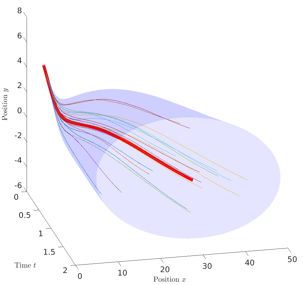
(a) Uncontrolled prior trajectory distribution

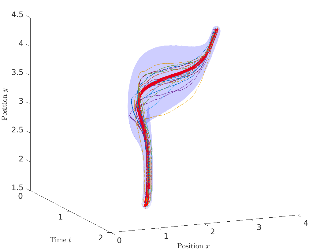
(b) Controlled trajectory distribution

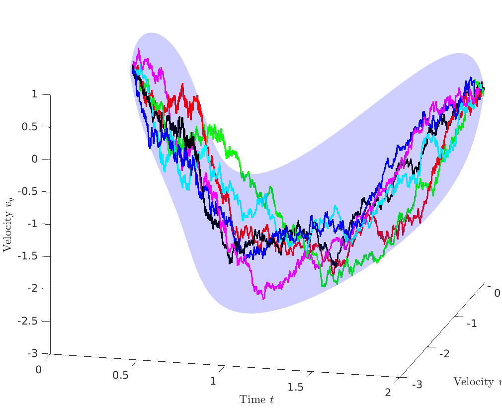
(c) Controlled velocity distribution

Figure 4: Visualization of trajectory distributions for uncontrolled (7) and controlled (29) LTV-SDE alongside sampled velocities. The system is obtained by linearizing the planar quadrotor model (33), with feedback control determined by solving PGCS-MP incorporating zero state cost. Mean trajectories are depicted in red, with the blue shading representing the $3-\sigma$ range of the covariance. The passive dynamics leads to an exploding behavior of the covariances while the feedback control guide the system to a desired terminal distribution. Girsanov theorem states that the KL-divergence between the two processes equals the expected control energy.

Theorem 3.

The optimal solution to the following problem is the solution to the Gaussian variational inference motion planning problem (16) over the same time discretization

$$\min_{X(\cdot),u(\cdot)}\!\!\!\!\!\!\!\!\! {\mathbb{E}}\{\int_{t_{0}}^{t_{N}}\frac{1}{2}\|u_{t}\|^{2}dt+\lVert\mathbf{h}(\mathbf{X})\rVert_{\Sigma_{\rm obs}}^{2}$$ (30b)

$$+\frac{1}{2}\lVert X_{0}-\!\mu_{0}\rVert_{K_{0}^{-1}}+\frac{1}{2}\lVert X_{N}-\mu_{N}\rVert_{K_{N}^{-1}}\}$$

$$dX_{t}=\!A_{t}X_{t}dt\!+\!a_{t}dt\!+\!B_{t}(u_{t}dt+dW_{t}).$$

Proof.

For the prior SDE (7), denote the probability density of the induced continuous-time path as $d{\mathbb{P}}^{0}$. Similarly, denote the probability density of the path induced by the controlled process (29) as $d{\mathbb{P}}^{u}$. Girsanov theorem introduced in section III-B states that the probability density ratio

$$\frac{d{\mathbb{P}}^{u}}{d{\mathbb{P}}^{0}}=\exp(\frac{1}{2}\int_{t_{0}}^{t_{N}}\lVert B_{t}u_{t}\rVert_{(B_{t}B_{t}^{T})^{\dagger}}^{2}dt+\int_{t_{0}}^{t_{N}}u_{t}^{T}dW_{t}),$$

from which we have

$${\rm{KL}}[d{\mathbb{P}}^{u}||d{\mathbb{P}}^{0}]=\int\log\frac{d{\mathbb{P}}^{u}}{d{\mathbb{P}}^{0}}d{\mathbb{P}}^{u}=\frac{1}{2\epsilon}{\mathbb{E}}\{\int_{t_{0}}^{t_{N}}\lVert u_{t}\rVert^{2}dt\}$$

for a full column rank $B_{t}$, due to the fact that ${\mathbb{E}}[w(\cdot)dW_{t}]=0,\forall w(\cdot),$ and $\lVert B_{t}u_{t}\rVert_{(B_{t}B_{t}^{T})^{\dagger}}^{2}=\lVert u_{t}\rVert^{2}$. We can thus rewrite the objective (30) into a distribution control problem

$$\min_{{\mathbb{P}}^{u}} \int[\log\frac{d{\mathbb{P}}^{u}}{d{\mathbb{P}}^{0}}+\lVert\mathbf{h}(\mathbf{X})\rVert_{\Sigma_{\rm obs}}^{2}+\frac{1}{2}\lVert X_{0}-\!\mu_{0}\rVert_{K_{0}^{-1}}$$

$$+\frac{1}{2}\lVert X_{N}-\mu_{N}\rVert_{K_{N}^{-1}}^{2}]d{\mathbb{P}}^{u},$$

which by definition of the KL-divergence, is equivalent to

$$\begin{split}\min_{{\mathbb{P}}^{u}}\;\;\;\;&{\mathbb{E}}\{\lVert\mathbf{h}(\mathbf{X})\rVert_{\Sigma_{\rm obs}}^{2}+\frac{1}{2}\lVert X_{0}-\!\mu_{0}\rVert_{K_{0}^{-1}}\\ &+\frac{1}{2}\lVert X_{N}-\mu_{N}\rVert_{K_{N}^{-1}}^{2}\}+{\rm{KL}}[d{\mathbb{P}}^{u}||d{\mathbb{P}}^{0}].\end{split}$$ (31)

Take time discretization $\mathbf{t}=[t_{0},\dots,t_{N}]$, the prior probability

$$d{\mathbb{P}}^{0}\approx\tilde{p}(\mathbf{X})\triangleq p(X_{1}|X_{0})\dots p(X_{N}|X_{N-1}).$$ (32)

The right hand side of (32) is a Gaussian distribution $\tilde{p}(\mathbf{X})\sim\mathcal{N}(\tilde{{\boldsymbol{\mu}}},\tilde{\mathbf{K}})$, and $\tilde{\mathbf{K}}^{-1}=\tilde{G}^{T}\tilde{Q}^{-1}\tilde{G}$, with [37]

$$\tilde{G}=\begin{bmatrix}-\Phi(t_{1},t_{0})&I&&&\\ &&\dots&&\\ &&&-\Phi(t_{N},t_{N-1})&I\end{bmatrix},$$

and

$$\tilde{Q}^{-1}={\rm diag}(Q_{0,1}^{-1},\ldots,Q_{N-1,N}^{-1}),$$

where $Q_{i,i+1}$ is the same Grammian as (12). The difference between $\tilde{p}(\mathbf{X})$ and $p(\mathbf{X})$ lies in the initial and terminal conditions $\mathcal{N}(\mu_{0},K_{0})$ and $\mathcal{N}(\mu_{N},K_{N})$. Adding boundary cost factors

$$\frac{1}{2}{\mathbb{E}}[\lVert X_{0}-\mu_{0}\rVert_{K_{0}^{-1}}^{2}],\;\;\frac{1}{2}{\mathbb{E}}[\lVert X_{N}-\mu_{N}\rVert_{K_{N}^{-1}}^{2}],$$

the joint distribution

$${\mathbb{E}}\{-\log d{\mathbb{P}}^{0}+\frac{1}{2}\lVert X_{0}-\mu_{0}\rVert_{K_{0}^{-1}}^{2}+\frac{1}{2}\lVert X_{N}-\mu_{N}\rVert_{K_{N}^{-1}}^{2}\}\\$$

coincides with (9). The joint probability of the discrete support states induced by controlled process $d{\mathbb{P}}^{u}$ is by definition also a Gaussian $d{\mathbb{P}}^{u}\approx\hat{q}(\mathbf{X})$. We thus arrive at the discrete approximation of the objective (31) as

$$\min_{\hat{q}\in\mathcal{\hat{Q}}}{\mathbb{E}}[\lVert\mathbf{h}(\mathbf{X})\rVert_{\Sigma_{\rm obs}}^{2}+{\rm{KL}}[\hat{q}({\mathbf{X})}||\mathcal{N}({\boldsymbol{\mu}},\mathbf{K})],$$

which coincide with the last line in GVI-MP formulation (16). ∎

Theorem 3 states that GVI-MP is equivalent to a stochastic feedback planning problem. The nominal trajectory in (30) is the stochastic prior (7), and the controlled dynamics also takes uncertainty into considerations. The objective in (28) is equivalent to minimizing the weighted distance of the next controlled support state to the reachable states resulting from passive dynamics

$$\lVert X_{t_{i+1}}-\mu_{t_{i+1}}-\Phi(t_{i+1},t_{i})(X_{i}-\mu_{t_{i}})\rVert_{Q_{i,i+1}^{-1}}^{2},$$

while in (30), the minimization of the expected stochastic control leads to its equivalence in minimizing the distance between the two processes (29) and (7) measured by ${\rm{KL}}[d{\mathbb{P}}^{u}||d{\mathbb{P}}^{0}]$.

To visualize the connections between inference and stochastic control, we offer two illustrative examples. In Figure 1, we depict the connection between GVI-MP and a stochastic control formulation for a 2-DOF point robot with linear dynamics. Figure 4 showcases uncontrolled and controlled LTV-SDE-based processes for a time-varying system, derived from linearized planar quadrotor dynamics [10]. The system operates within a 6-dimensional state space denoted as $X_{t}=[p_{x},p_{z},\phi,v_{x},v_{z},\dot{\phi}]$. Here, $(p_{x},p_{z})$ signify global lateral and vertical positions, while $(v_{x},v_{z})$ stand for lateral and vertical velocities in the body frame, with $\phi$ accounting for the singular rotational degree of freedom

$$\dot{X_{t}}=\begin{bmatrix}v_{x}\cos(\phi)-v_{z}\sin(\phi)\\ v_{x}\sin(\phi)+v_{z}\cos(\phi)\\ \dot{\phi}\\ v_{z}\dot{\phi}-g\sin(\phi)\\ -v_{x}\dot{\phi}-g\cos(\phi)\\ 0\end{bmatrix}+\begin{bmatrix}0&0\\ 0&0\\ 0&0\\ 0&0\\ 1/m&1/m\\ l/J&-l/J\end{bmatrix}\begin{bmatrix}u_{1}\\ u_{2}\end{bmatrix}.$$ (33)

V-C Linear covariance steering for general nonlinear state cost

The stochastic control formulation (30) represents a classical terminal-cost-based regulator problem, amenable to iterative techniques like iLQG. However, our focus lies in tackling a more intricate constrained variant with the same running costs. This demanding constrained GVI problem aligns precisely with covariance steering [20, 21, 22].

a) Covariance steering formulation. We consider the covariance steering problem with nonlinear state costs as

$$\min_{u} {\mathbb{E}}\left\{\int_{0}^{T}[\frac{1}{2}\|u_{t}\|^{2}+V(X_{t})]dt\right\}$$ (34c)

$$dX_{t}=A_{t}X_{t}dt+a_{t}dt+B_{t}(u_{t}dt+\sqrt{\epsilon}dW_{t})$$

$$X_{0}\sim\mathcal{N}(\mu_{0},K_{0}),\quad X_{T}\sim\mathcal{N}(\mu_{T},K_{T}).$$

Note that (34) is nonlinear in the sense that the state cost $V(X_{t})$ is nonlinear. We use $(0,T)$ to emphasize the continuous-time nature.

Let the state cost $V(X_{t})$ be

$$V(X_{t})=\lVert\mathbf{h}(X_{t})\rVert_{\Sigma_{\rm obs}}^{2},$$ (35)

then formulation (34) is equivalent to the stochastic control problem (30) with a constraint. We also inject a noise intensity $\epsilon$ in (34) compared with (30).

b) Quadratic approximation of the nonlinear cost. Using Girsanov theorem, (34) is equivalent to the distributional control

$$\min_{{\mathbb{P}}^{u}} \int d{\mathbb{P}}^{u}\left[\log\frac{d{\mathbb{P}}^{u}}{d{\mathbb{P}}^{0}}+\frac{1}{\epsilon}V\right]$$ (36c)

$$(X_{0})_{\sharp}{\mathbb{P}}^{u}=\mathcal{N}(\mu_{0},K_{0})$$

$$(X_{T})_{\sharp}{\mathbb{P}}^{u}=\mathcal{N}(\mu_{T},K_{T}),$$

where $(\cdot)_{\sharp}{\mathbb{P}}^{u}$ is the push-forward operator induced by ${\mathbb{P}}^{u}$.

Problem (36) is an optimization over the space ${\mathbb{P}}^{u}$. We thus parameterize the search space $\hat{\Pi}(\rho_{0},\rho_{T})$ as the one that is induced by a parameterized linear Gauss Markov process

$$dX_{t}=A_{t}^{k}X_{t}dt+a_{t}^{k}dt+\sqrt{\epsilon}B_{t}dW_{t}.$$ (37)

At iteration $k$, we use $z_{t}$ to represent the mean trajectory of ${\mathbb{P}}^{k}$ which is induced by the process (37). We approximate the state cost by a quadratic function

$$\hat{V}(t,x)\approx V(z_{t})+(x^{T}-z_{t}^{T})\nabla V+\frac{1}{2}(x^{T}-z_{t}^{T})\nabla^{2}V(x-z_{t}).$$ (38)

c) Composite optimization scheme. Proximal gradient method [45] solves a composite optimization problem by splitting the objective (36c) into

$$\min_{{\mathbb{P}}^{u}\in\Pi(\rho_{0},\rho_{T})}F({\mathbb{P}}^{u})+G({\mathbb{P}}^{u}),$$ (39)

where

$$F({\mathbb{P}}^{u})=\int[\frac{1}{\epsilon}V-\log d{\mathbb{P}}^{0}]d{\mathbb{P}}^{u},\;\;G({\mathbb{P}}^{u})=\int d{\mathbb{P}}^{u}\log d{\mathbb{P}}^{u}.$$

Proximal gradient is an optimization paradigm where only $F$ is required to be smooth, the function $G$ does not have to be differentiable. In the Euclidean spaces, for variable $y$, the algorithm follows the update

$$y^{k+1}\operatorname*{argmin}_{y\in{\mathcal{Y}}}G(y)\!+\!\frac{1}{2\eta}\|y\!-\!y^{k}\|^{2}\!\!+\!\!\langle\nabla F(y^{k}),y\!-\!y^{k}\rangle.$$ (40)

The proximal gradient for non-Euclidean distances is built upon the mirror descent method [46, 45]. In (40), the vector norm can be replaced by a Bregman divergence $D(\cdot,\cdot)$, and the generalized non-Euclidean proximal gradient update is

$$y^{k+1}=\operatorname*{argmin}_{y\in{\mathcal{Y}}}G(y)+\frac{1}{\eta}D(y,y^{k})+\langle\nabla F(y^{k}),y-y^{k}\rangle.$$

The KL divergence is often a choice for $D(\cdot,\cdot)$ for distributions, and the proximal gradient step is then obtained from

$${\mathbb{P}}_{k+1}=\operatorname*{argmin}_{{\mathbb{P}}^{u}\in\hat{\Pi}(\rho_{0},\rho_{T})}G({\mathbb{P}}^{u})+\frac{1}{\eta}{\rm KL}({\mathbb{P}}^{u}\|{\mathbb{P}}_{k})+\langle\frac{\delta F}{\delta{\mathbb{P}}}({\mathbb{P}}_{k}),{\mathbb{P}}^{u}\rangle.$$ (41)

d) Proximal update for quadratic state cost. With the approximated cost (38), each step of proximal gradient (41) amounts to solving the approximated distributional control

$$\min_{{\mathbb{P}}^{u}\in\hat{\Pi}(\rho_{0},\rho_{T})}\int[\frac{1}{\epsilon}\hat{V}-\log d{\mathbb{P}}^{0}]d{\mathbb{P}}^{u}+\int d{\mathbb{P}}^{u}\log d{\mathbb{P}}^{u},$$ (42)

and the component $F({\mathbb{P}}^{u})$ in (39) becomes

$$F({\mathbb{P}}^{u})=\int[\frac{1}{\epsilon}\hat{V}-\log d{\mathbb{P}}^{0}]d{\mathbb{P}}^{u}=\langle\frac{1}{\epsilon}\hat{V}-\log d{\mathbb{P}}^{0},{\mathbb{P}}^{u}\rangle.$$ (43)

We denote $\frac{\delta F}{\delta{\mathbb{P}}}$ as the variation of $F({\mathbb{P}})$ with respect to a small variation $\delta{\mathbb{P}}$. Before deriving the expressions for $\frac{\delta F}{\delta{\mathbb{P}}}$, we distinguish 3 different trajectory distributions:

1. Distribution ${\mathbb{P}}^{0}$ induced by the passive dynamics (7).

2. Distribution ${\mathbb{P}}_{k}$ induced by the controlled dynamics (37) at the current iteration $k$.

3. Dandidate distribution ${\mathbb{P}}^{u}$ in solution space $\hat{\Pi}(\rho_{0},\rho_{T})$.

V-D Main Algorithm

We remark first that in all the derivations that follow, the gradients and the Hessians of $V$ are evaluated on the nominal mean trajectory, and all the gradients are with respect to the state vector $X_{t}$, i.e., $\nabla V\triangleq\nabla_{X}V(z_{t}),\;\;\nabla^{2}V\triangleq\nabla_{X}^{2}V(z_{t}).$

Lemma 4.

Let ${\mathbb{P}}$ be the path distribution induced by a Gauss Markov process (7), then the variation of $F({\mathbb{P}})$ w.r.t. ${\mathbb{P}}$ for linear dynamics (34) is

$$\frac{\delta F}{\delta{\mathbb{P}}}({\mathbb{P}})=\frac{1}{\epsilon}\hat{V}-\log d{\mathbb{P}}^{0}+\frac{1}{2\epsilon}x^{T}\nabla\operatorname{Tr}(\nabla^{2}V\Sigma_{t}).$$ (44)

Proof.

See Appendix -D. ∎

Next write the objective of the proximal gradient update step (41) using (44). We drop the dependences on time $t$ and iteration $k$ for notation simplicity. The objective in (41) is

$$\int[\frac{1}{\epsilon}\hat{V}+\frac{1}{2\epsilon}x^{T}\nabla\operatorname{Tr}((\nabla^{2}V)\Sigma)]d{\mathbb{P}}+{\rm KL}({\mathbb{P}}\|{\mathbb{P}}^{0})+\frac{1}{\eta}{\rm KL}({\mathbb{P}}\|{\mathbb{P}}^{u}),$$ (45)

where we just combined the term $-\int\log d{\mathbb{P}}^{0}d{\mathbb{P}}$ in (42) with $G({\mathbb{P}}^{u})=\int d{\mathbb{P}}^{u}\log d{\mathbb{P}}^{u}$ to form

$$G({\mathbb{P}}^{u})-\int\log d{\mathbb{P}}^{0}d{\mathbb{P}}^{u}=\int\log\frac{d{\mathbb{P}}^{u}}{d{\mathbb{P}}^{0}}\log d{\mathbb{P}}^{u}={\rm KL}({\mathbb{P}}^{u}||{\mathbb{P}}^{0}).$$

Next, we show that each step in the proximal gradient covariance steering is to solve a linear covariance steering problem.

Theorem 5.

Each step of the proximal gradient covariance steering (41) is obtained by solving the following linear covariance steering

$$\min_{u}\!\!\!\! \!\!\!\!{\mathbb{E}}\left\{\int_{0}^{T}[\frac{1}{2}\|u_{t}\|^{2}+\frac{1}{2}X_{t}^{T}Q_{t}^{k}X_{t}+X_{t}^{T}r_{t}^{k}]dt\right\}$$ (46c)

$$\!\!\!\!dX_{t}=\bar{A}_{t}^{k}X_{t}dt+\bar{a}_{t}^{k}dt+B_{t}(u_{t}dt+\sqrt{\epsilon}dW_{t})$$

$$X_{0}\sim\mathcal{N}(\mu_{0},K_{0}),\quad X_{T}\sim\mathcal{N}(\mu_{T},K_{T}),$$

where

$$\bar{A}_{t}^{k} =\frac{1}{1+\eta}[A_{t}^{k}+\eta A_{t}]$$ (47a)

$$\bar{a}_{t}^{k} =\frac{1}{1+\eta}[a_{t}^{k}+\eta a_{t}]$$ (47b)

$$Q_{t}^{k} =\frac{\eta}{1+\eta}\nabla^{2}V+\frac{\eta}{(1+\eta)^{2}}(A_{t}^{k}-A_{t})^{T}(B_{t}B_{t}^{T})^{\dagger}(A_{t}^{k}-A_{t})$$ (47c)

$$r_{t}^{k} =\frac{\eta}{1+\eta}\nabla V+\frac{\eta}{2(1+\eta)}[\nabla\operatorname{Tr}(\nabla^{2}V\Sigma^{k}_{t})-2\nabla^{2}Vz^{k}_{t}]$$

$$\hskip 14.22636pt+\frac{\eta}{(1+\eta)^{2}}(A_{t}^{k}-\hat{A}_{t}^{k})^{T}(B_{t}B_{t}^{T})^{\dagger}(a_{t}^{k}-\hat{a}_{t}^{k}),$$ (47d)

where $(\cdot)^{\dagger}$ represents pseudo-inverse, $z^{k}_{t}$ and $\Sigma^{k}_{t}$ are the mean and covariance of ${\mathbb{P}}_{k}$, respectively.

Proof.

See Appendix -E. ∎

Problem (46) is a linear covariance steering problem that admits a closed-form solution as mentioned in section III-C,

$$u_{t}^{\star}=K_{t}^{k}X_{t}+d_{t}^{k},$$

due to which the next-iteration Gauss Markov process follows

$$A_{t}^{k+1}=\bar{A}_{t}^{k}+B_{t}K_{t}^{k},\;\;\;\;a_{t}^{k+1}=\bar{a}_{t}^{k}+B_{t}d_{t}^{k}.$$ (48)

The path distribution ${\mathbb{P}}_{k}$ is always induced by a Gauss-Markov process without explicit control. The nominal trajectory $(z_{t}^{k},\Sigma_{t}^{k})$ thus evolves as

$$\dot{z}_{t}^{k}=A_{t}^{k}z_{t}^{k}+a_{t}^{k},\;\;\dot{\Sigma}_{t}^{k}=A_{t}^{k}\Sigma_{t}^{k}+\Sigma_{t}^{k}(A_{t}^{k})^{T}+\epsilon B_{t}B_{t}^{T}.$$ (49)

On top of the basic optimization scheme, we also add a backtracking procedure to select the step sizes. For computation efficiency, we compute the collision costs using only the nominal trajectories in the backtracking.

1

input : Number of iterations $I_{M}$, noise $\epsilon$, stepsize $\eta$, backtrack ratio $\beta$, Number of backtrack $M_{\beta}$, Signed distance field $SDF$.

output : Optimized nominal $(z_{t}^{*},\Sigma_{t}^{*})$ and feedback gain $(K_{t}^{*},d_{t}^{*})$.

2

3Initialize time-varying $(A_{t}^{0},a_{t}^{0},z_{t}^{0},\Sigma_{t}^{0})$ and cost $V_{0}$.

4for $k=1,2,\dots$, $I_{M}$ do

5       Step size $\tilde{\eta}\leftarrow\eta$.

6      for $j=1,2,\dots,M_{\beta}$ do

7             $(\tilde{z}_{t}^{k},\tilde{\Sigma}_{t}^{k})\leftarrow$ Propagate$(z_{t}^{k},\Sigma_{t}^{k})$ (49).

8            $(\bar{A}_{t}^{k},\bar{a}_{t}^{k},Q_{t}^{k},r_{t}^{k})\leftarrow$ ComputeQr

9             (47).

10            $(\tilde{K}_{t}^{k},\tilde{d}_{t}^{k})\leftarrow$ LinearCovarianceSteering (46).

11            $\tilde{V}_{k}\leftarrow$ ComputeCosts$(\tilde{z}_{t}^{k},\tilde{\Sigma}_{t}^{k},\tilde{K}_{t}^{k},\tilde{d}_{t}^{k},SDF)$.

12            if $\tilde{V}_{k}<V_{k-1}$ or $j==M_{\beta}$ then

13                   $V_{k}\leftarrow\tilde{V}_{k}.$

14                  $(A_{t}^{k},a_{t}^{k})\leftarrow$ Update $(\bar{A}_{t}^{k},\bar{a}_{t}^{k},\tilde{K}_{t}^{k},\tilde{d}_{t}^{k})$ (48).

15                  Break;

16             end if

17            $\tilde{\eta}\leftarrow\beta\times\tilde{\eta}.$

18       end for

19      if  $k==I_{M}$ or $0<V_{k-1}-V_{k}<\epsilon$ then

20             $K_{t}^{*}\leftarrow K_{t}^{k},\;d_{t}^{*}\leftarrow d_{t}^{k},\;z_{t}^{*}\leftarrow z_{t}^{k},\Sigma_{t}^{*}\leftarrow\Sigma_{t}^{k}.$

21       end if

22      

23 end for

Algorithm 2 Proximal Gradient Covariance Steering Motion Planning (PGCS-MP)

We introduce the PGCS-MP algorithm in Algorithm 2. Line $2$ is the main iteration loop for proximal gradient updates, where the step size is initialized to $\eta$ during the backtracking procedure at line $3$. The subsequent for-loop in line $4$ governs the backtracking. Initially, the nominal trajectory is propagated through (49), followed by the calculation of $(\bar{A}_{t}^{k},\bar{a}_{t}^{k},Q_{t}^{k},r_{t}^{k})$ for linear covariance steering within each proximal gradient step, as detailed in (47). Subsequently, line $7$ solves the linear covariance steering problem (46). Line $9-15$ conduct the backtracking process.

VI experiments

We demonstrate simulated experiment results to validate the proposed algorithms. When evaluating the signed distance function, robots are modeled as balls with fixed radius $r$ [7] at designated locations. The minimum distance from robots to obstacles is efficiently computed using the distance between centers of the balls to the obstacles and the ball radius.

We assume the linear stochastic dynamical system [7] [35]

$$dX_{t}=A_{t}X_{t}dt+a_{t}dt+B_{t}(u_{t}dt+dW_{t}),$$

where $A_{t},a_{t},B_{t}$ are under a constant velocity dynamics assumption

$$A_{t}=\begin{bmatrix}0&I\\ 0&0\end{bmatrix},~{}a_{t}=\begin{bmatrix}0\\ 0\end{bmatrix},~{}B_{t}=\begin{bmatrix}0\\ I\end{bmatrix}.$$ (50)

For this dynamics, the transition matrix $\Phi$, matrices $Q_{i,i+1}^{-1}$, $Q^{-1}$, and $G$ in (11) and (10) can be calculated explicitly [37].

VI-A Point robots

We first evaluate the proposed methods on a point robot model.

a) 2D point robot

We first consider the 2-dimensional point robot motion planning in an obstacle-cluttered environment. We conduct 4 experiments with different start and goal states defined as

$$\begin{split}X_{0}^{1}&=[7,-5,0,0],\;\;X_{T}^{1}=[-10,17,0,0];\\ X_{0}^{2}&=[-7,-5,0,0],\;\;X_{T}^{2}=[8,18,0,0];\\ X_{0}^{3}&=[-7,-5,0,0],\;\;X_{T}^{3}=[13,10,0,0];\\ X_{0}^{4}&=[13,14,0,0],\;\;X_{T}^{4}=[-12,7,0,0].\end{split}$$

The results of both GVI-MP and PGCS-MP are shown in figure 5. Both algorithms find collision-free trajectory distributions in all the $4$ different experiment settings. The GVI-MP results are obtained from a two-phase optimization, i.e., low temperature and high temperature as mentioned in section IV-B. Under the principle of maximum entropy motion planning objectives, the results spread wide in the feasible region in the environments, as compared with the PGCS-MP results.

However, we examine the terminal covariances to validate the performance of the PGCS-MP algorithm in solving the constrained covariance steering formulation (34). We remark that if we put smaller soft boundary penalties

$$\frac{1}{2}{\mathbb{E}}[\lVert X_{0}-\mu_{0}\rVert_{K_{0}^{-1}}^{2}],\;\;\frac{1}{2}{\mathbb{E}}[\lVert X_{N}-\mu_{N}\rVert_{K_{N}^{-1}}^{2}],$$

in GVI-MP or GPMP2, the terminal constraints may be violated. In PGCS-MP, the terminal covariance is guaranteed by the hard constraint in the formulaiton. In all the experiments in Figure 5(b), we set the initial covariance to be 0.01$I$ and the terminal covariances are constrained to be 0.05$I$. To verify the satisfaction of the boundary conditions, we record the solved terminal covariances in the four cases, which are

$$\Sigma_{T}^{*}=\begin{bmatrix}0.0499&0&0.0003&0\\ 0&0.0499&0&0.0003\\ 0.0003&0&0.0500&0\\ 0&0.0003&0&0.0500\end{bmatrix}$$

in all the 4 experiments. For the continuous-time covariance control formulation, there are several numerical integrations including solving the Ricatti equations (6), computing the state transition matrix, and the propagation of the nominal trajectories $z_{t}$ in (49). We used a second-order numerical integration scheme known as Heun’s method [47] for all the numerical integrations encountered.

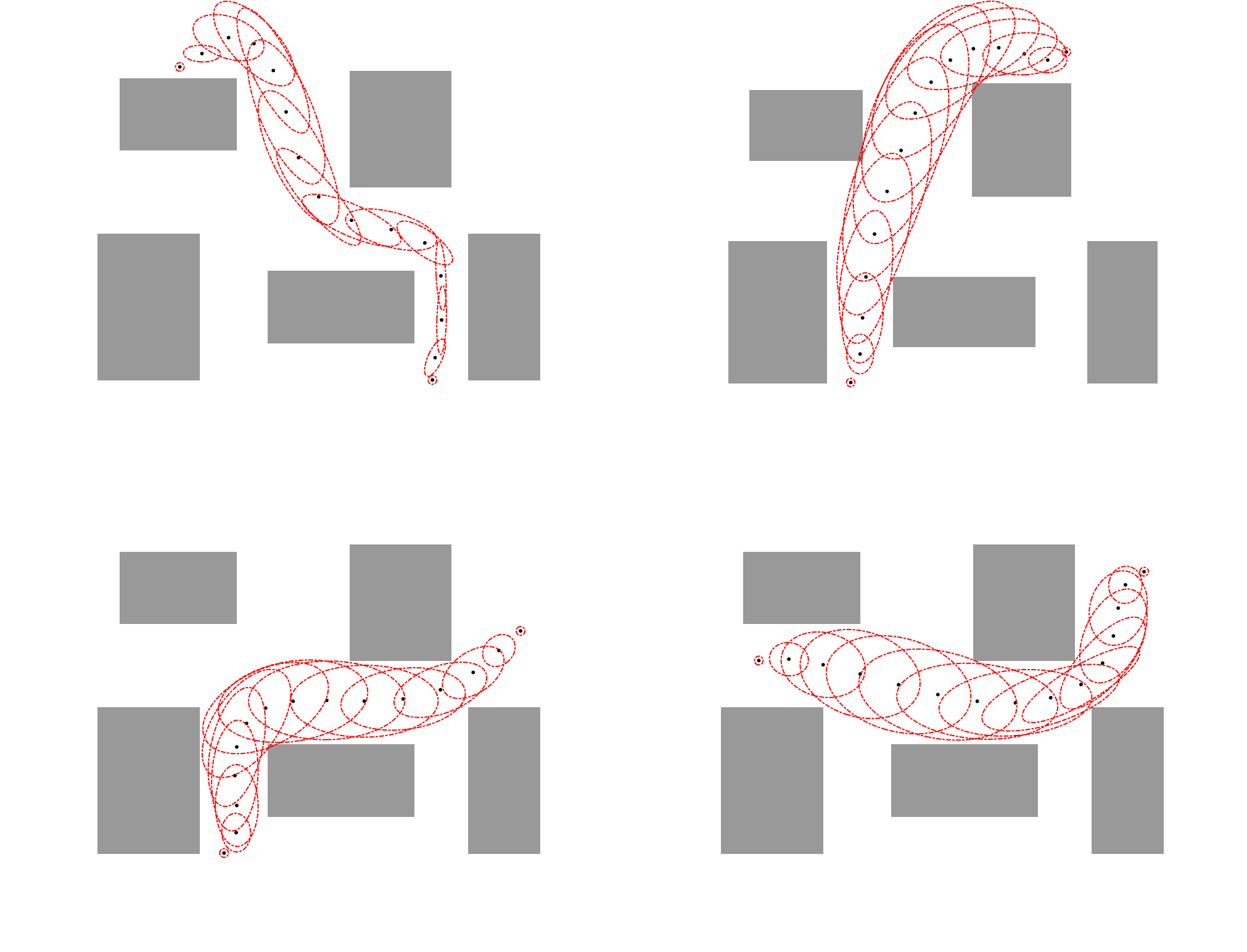
(a) Motion planning for 2d point robot, GVI-MP.

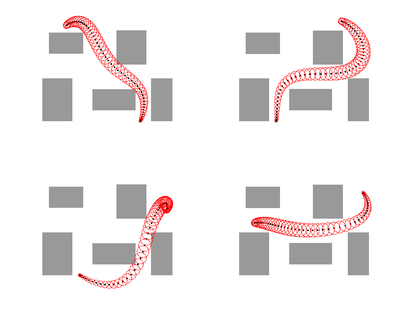
(b) Motion planning for 2d point robot, PGCS-MP.

Figure 5: Motion planning for 2D Point Robot obtained from GVI-MP and PGCS-MP algorithms with same environment and tasks. 15 Support states are used for GVI-MP, and 50 support states are used for PGCS-MP. For comparison, for GVI-MP we put large boundary-violating penalties, while for the PGCS-MP we set a large terminal covariance constraint to show the advantage of the constrained formulation (36) compared with the GVI-MP formulation with terminal costs (30).

b) 3D point robot We conduct experiments for a 3-DOF point robot in a cluttered environment using PGCS-MP. The start and goal states are

$$\begin{split}X_{0}^{1}&=[-10,10,0,0,0,0],\;\;X_{T}^{1}=[35,35,27,0,0,0];\\ X_{0}^{2}&=[-11,-11,0,0,0,0],\;\;X_{T}^{2}=[30,35,30,0,0,0];\\ X_{0}^{3}&=[30,-10,-5,0,0,0],\;\;X_{T}^{3}=[-10,20,15,0,0,0];\\ X_{0}^{4}&=[-10,25,0,0,0,0],\;\;X_{T}^{4}=[30,-15,30,0,0,0].\end{split}$$

The results are shown in figure 6. In all 4 experiment settings, the PGCS-MP algorithm is able to find collision-free trajectory distributions.

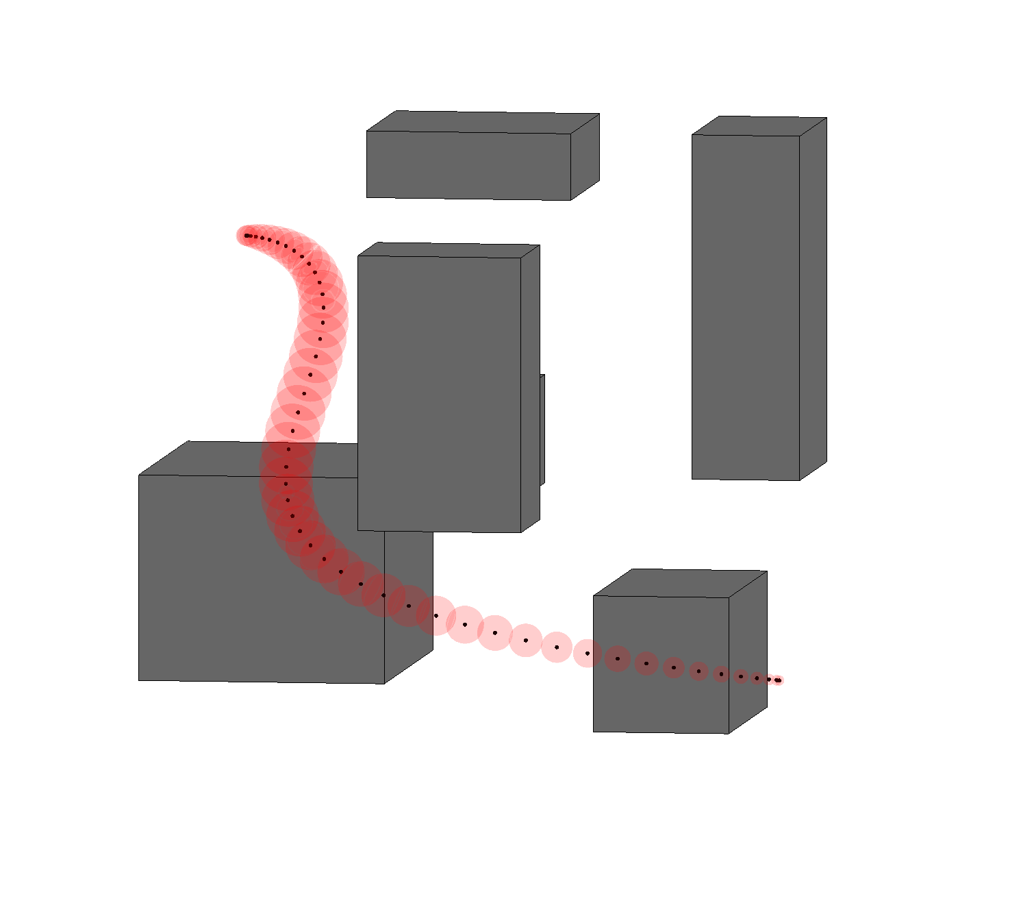
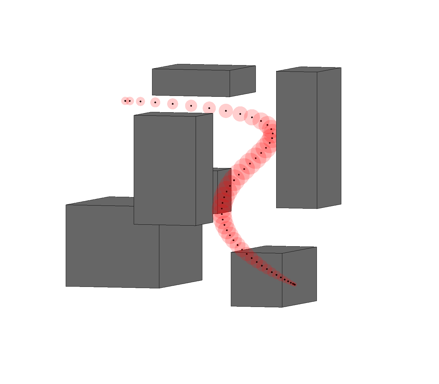
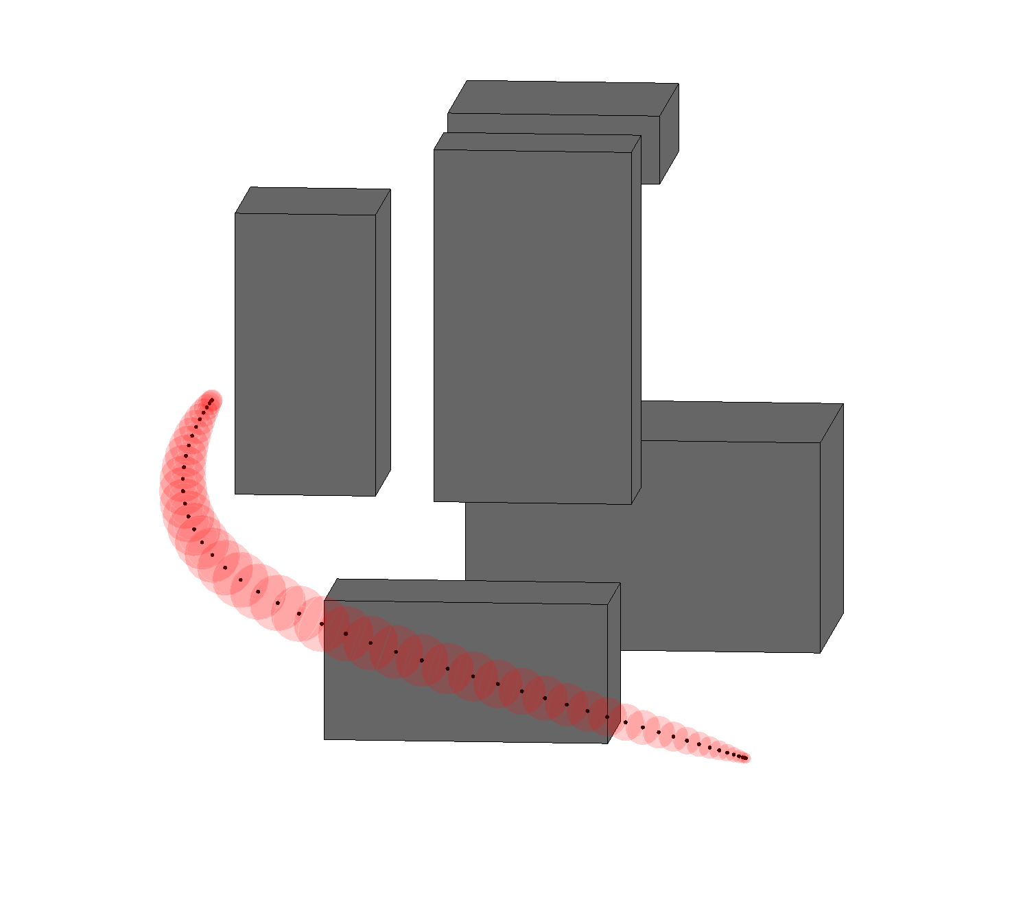
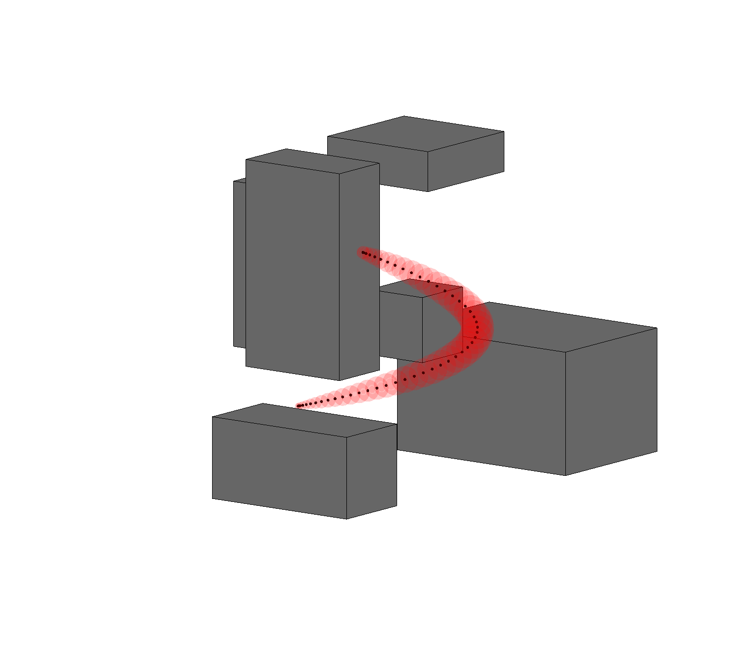
Figure 6: Motion planning for 3D robot, PGCS-MP.

VI-B Arm robots

We next validate the proposed methods for arm robots. We first show the results for a simple 2-link arm motion planning task, then we extend the scale to a 7-DOF WAM robot arm in a more realistic environment.

a) 2-link Arm. We applied the two proposed algorithms on a 2-DOF arm robot in a collision avoidance motion planning task. The start and goal states are

$$X_{0}=[0,0,0,0],\;\;X_{T}=[0,\frac{\pi}{2},0,0].$$

We plot the motion plans from both GPMP2, GVI-MP, and PGCS-MP in figure 7. Compared with the deterministic baseline motion plan, we show in figure 8 the mean and the sampled support states from the obtained trajectory distributions.

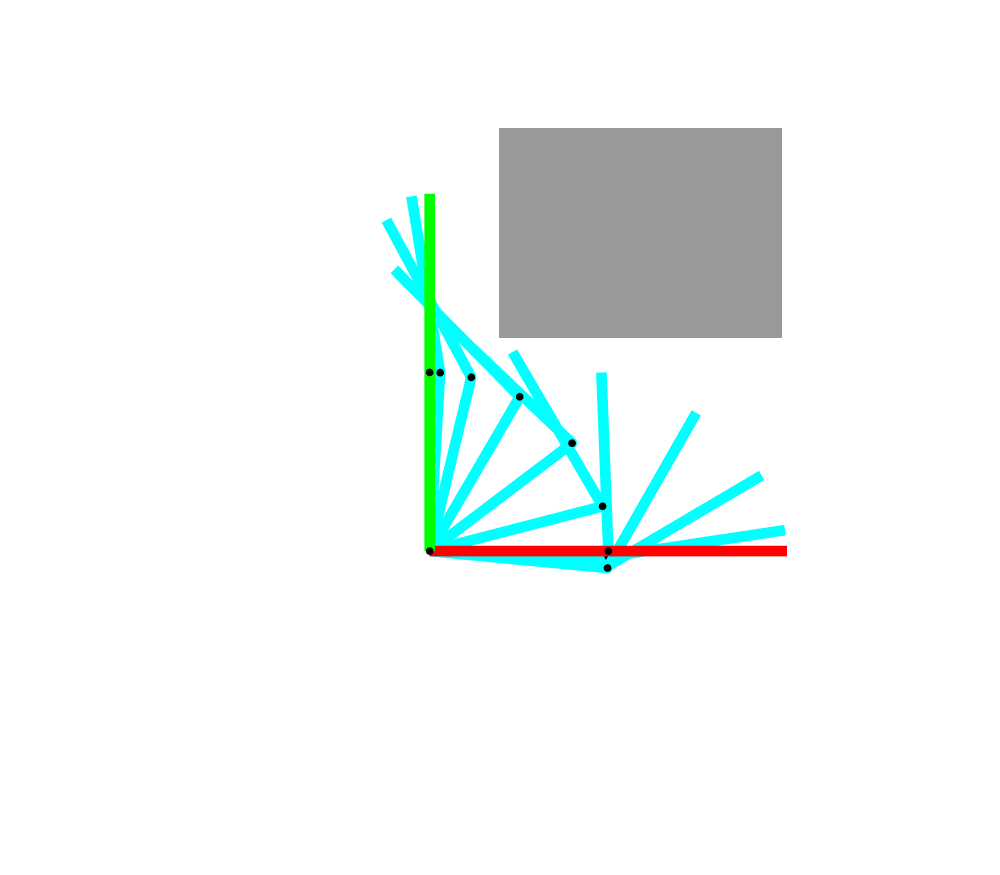
(a) GPMP2 Result

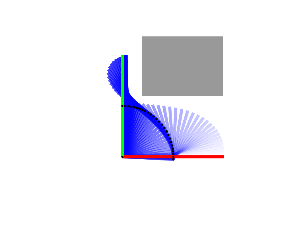
(b) GVI-MP Mean

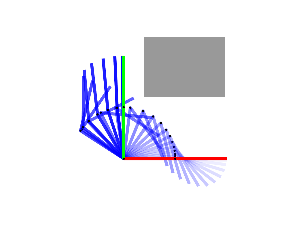
(c) PGCS-MP Mean

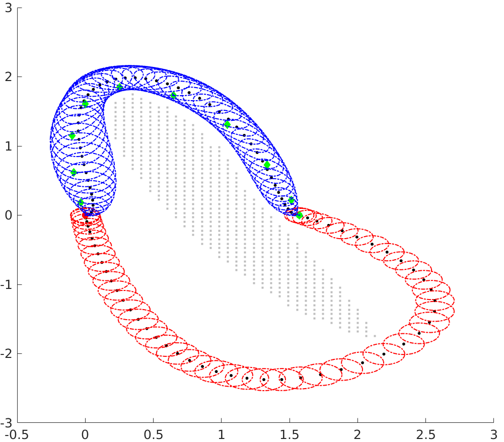
(d) Configuration space

Figure 7: Motion planning for 2-link arm in an environment with one obstacle. Subfigure 7(d) shows the obstacle and trajectories in configuration space. The green dots in diamond shape are GPMP2 trajectory, the blue ellipsoids are the covariances of the GVI-MP trajectory distribution, and the red ellipsoids are the covariances of PGCS-MP trajectory distribution.

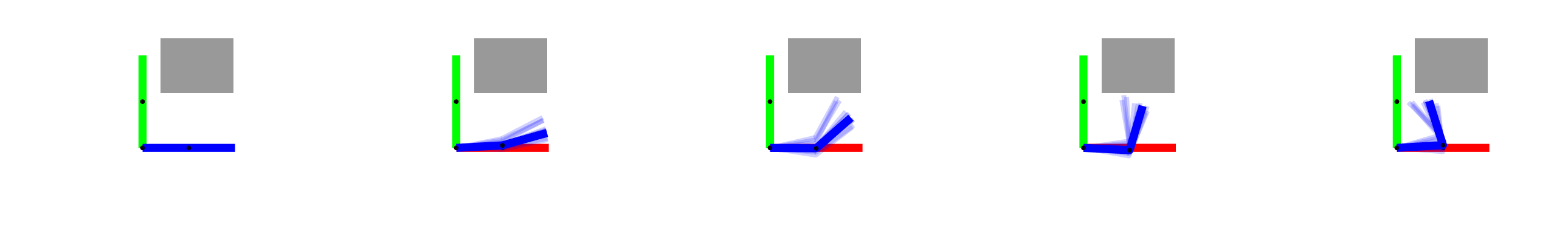
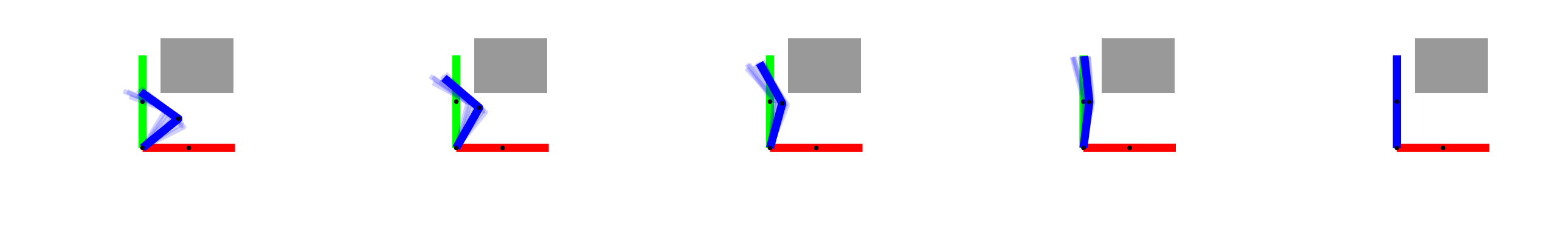
(a) Mean and sampled trajectory for GVI-MP

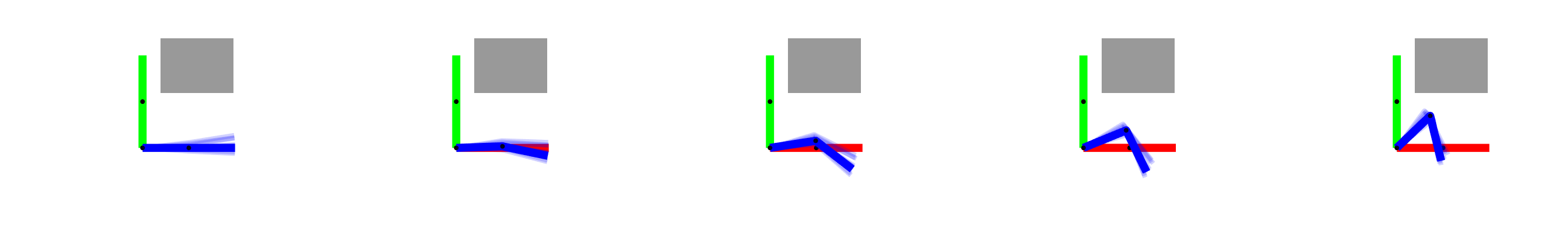
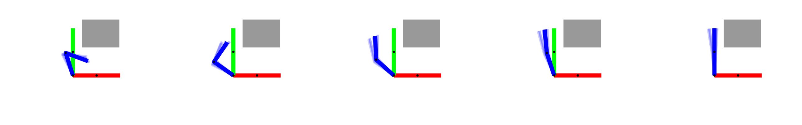
(b) Mean and sampled trajectory for PGCS-MP

Figure 8: Mean and sampled trajectories from the trajectory distributions.

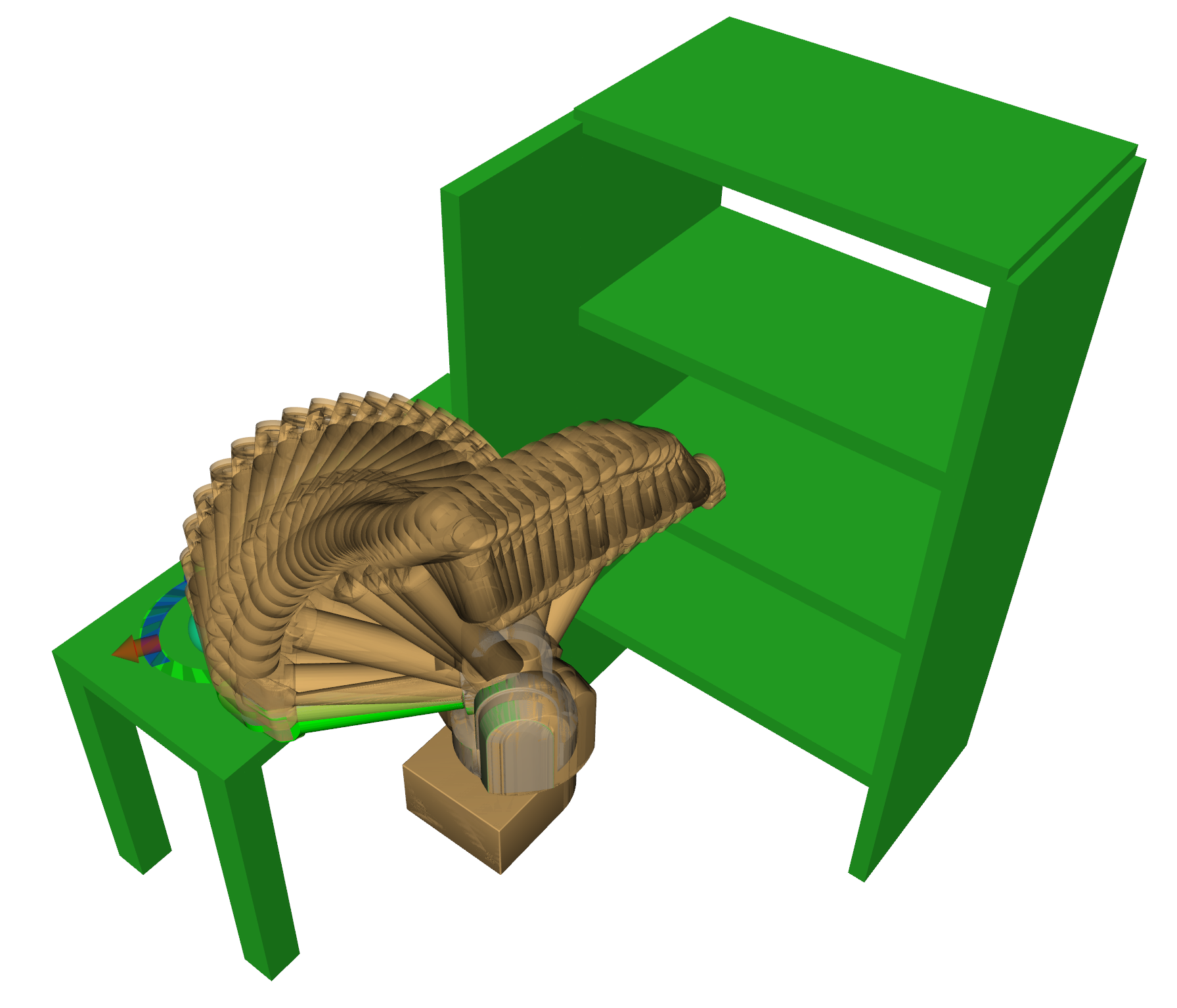
(a) GPMP2

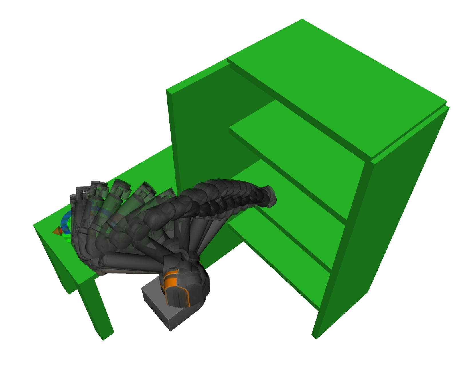
(b) GVI-MP mean

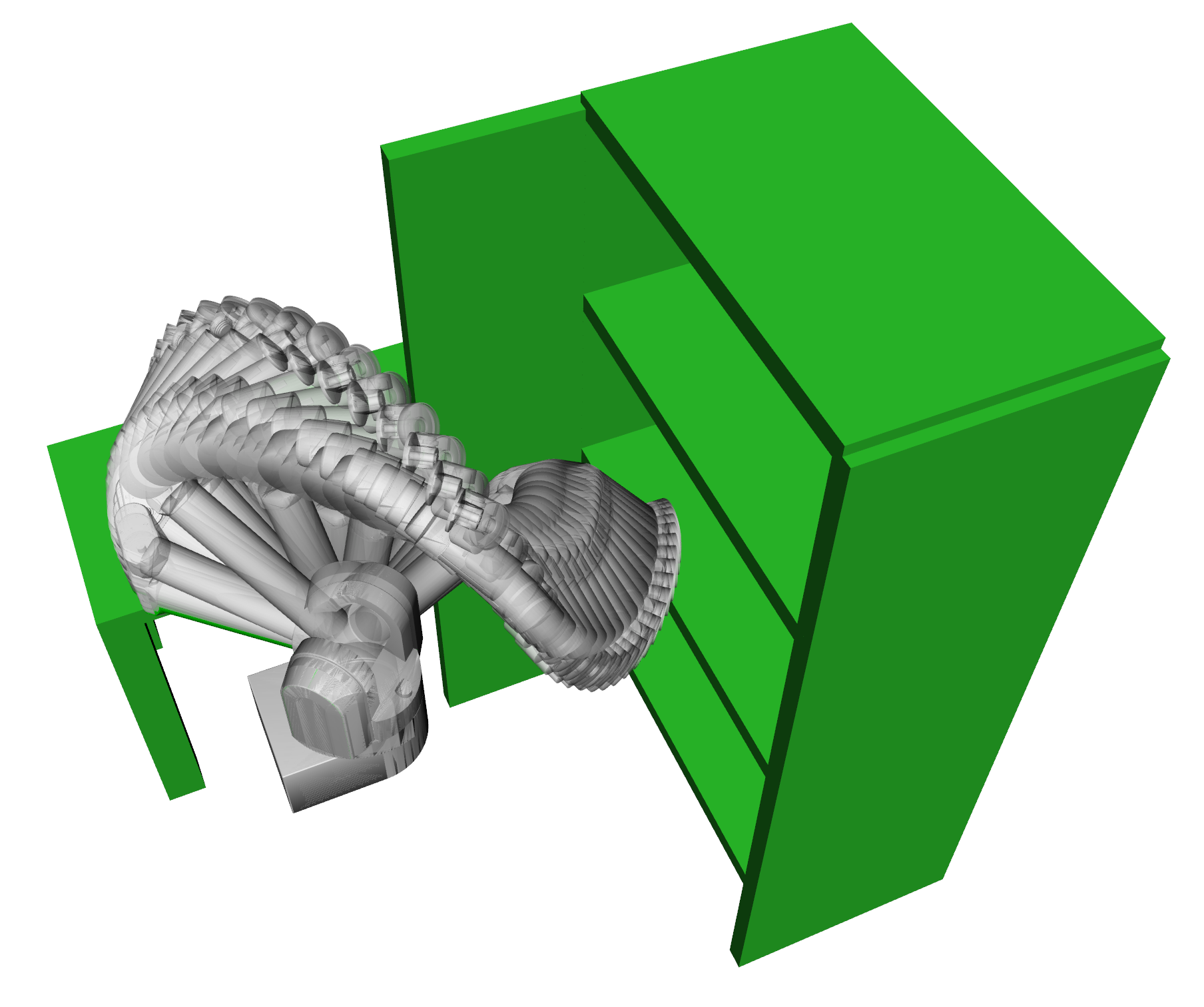
(c) PGCS-MP mean

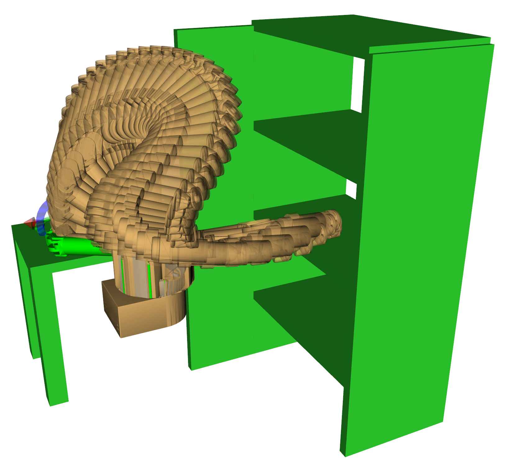
(d) GPMP2

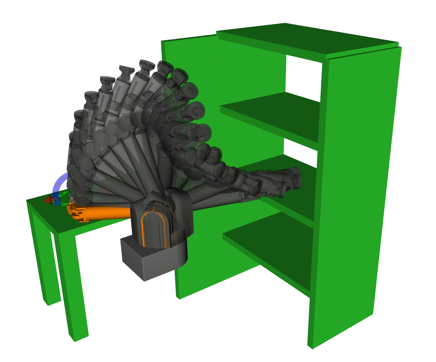
(e) GVI-MP mean

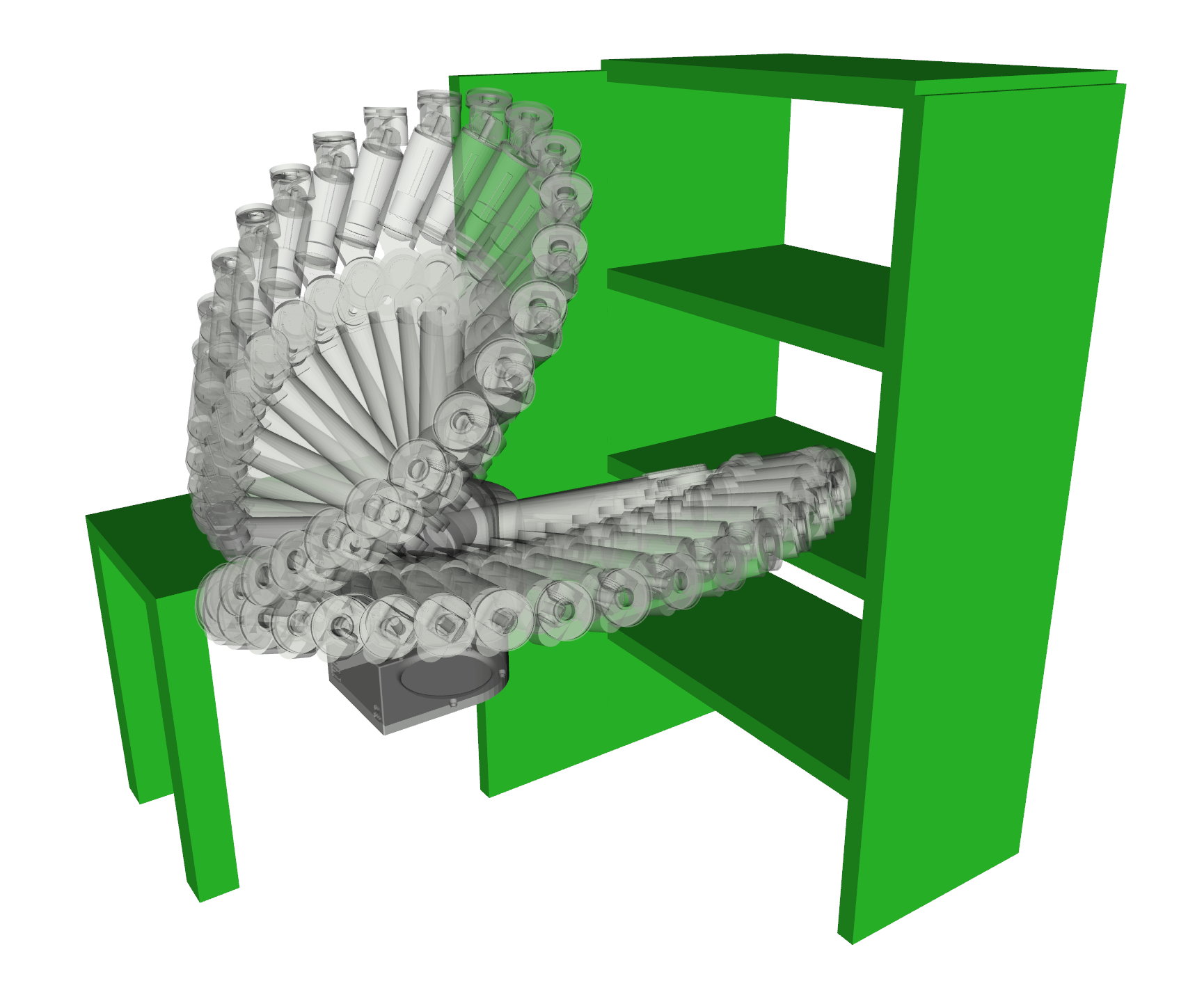
(f) PGCS-MP mean

Figure 9: Motion planning for a 7-DOF WAM Arm using the proposed two algorithms for two tasks, one on each row. All results are visualized using a WAM robot URDF in ROS moveit! [48] environment and are compared with the gpmp2 baseline.

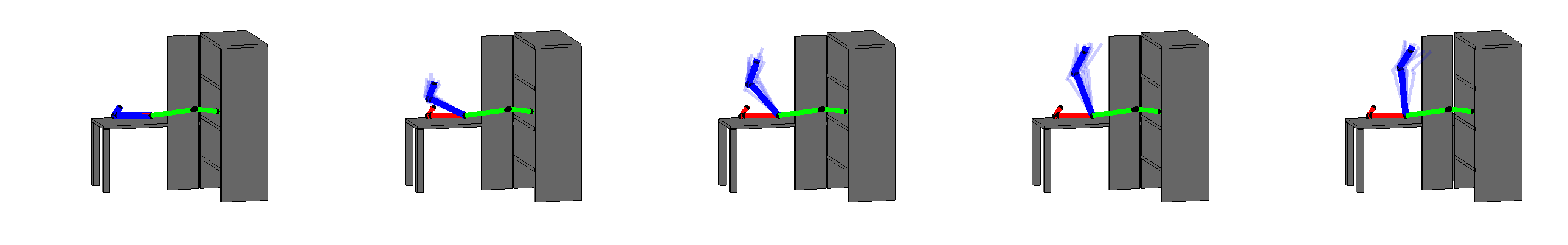
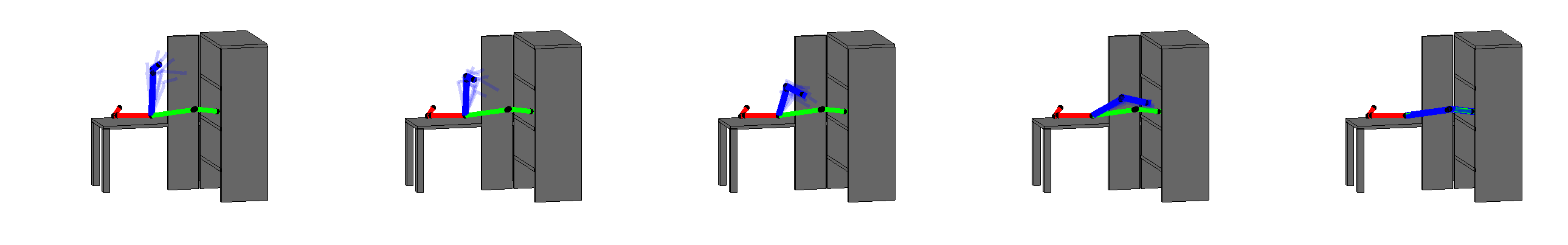
(a) GVI-MP mean and sampled trajecotries.

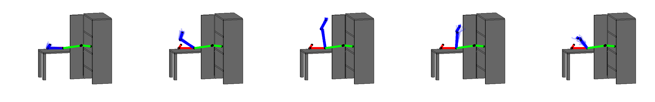
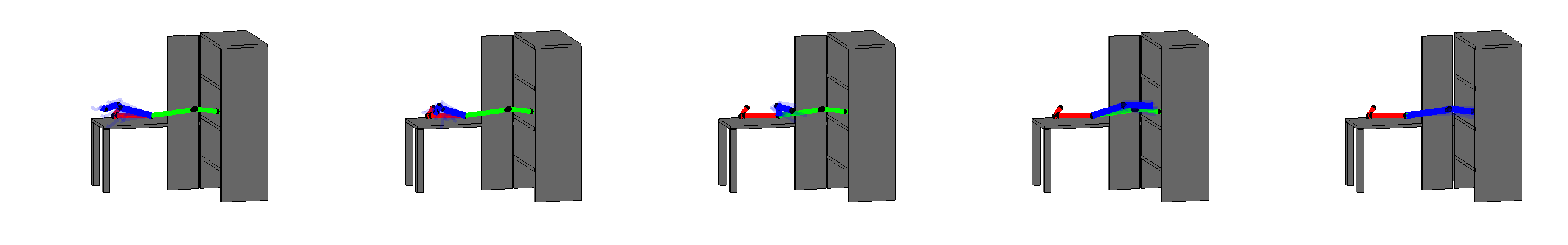
(b) PGCS-MP mean and sampled trajecotries.

Figure 10: Mean and sampled trajecotries for the two algorithms for the second experiment in figure 9.

b) 7-DOF WAM Arm. We next conduct experiments for a 7-DOF WAM robot arm in a bookshelf environment. In the first experiment, the start and goal joint angles are

$$\begin{split}P_{0}^{1}&=[-0.8,-1.70,1.64,1.29,1.1,-0.106,2.2],\\ P_{T}^{1}&=[-0.0,0.94,0.00,1.6,0.0,-0.919,1.55],\end{split}$$

and for the second experiment

$$\begin{split}P_{0}^{2}&=[-0.9,-1.70,1.34,1.19,0.8,-0.126,2.5],\\ P_{T}^{2}&=[-0.7,1.35,1.2,1.0,-0.7,-0.1,1.2].\end{split}$$

The start and goal velocities for the 2 experiments are all set to zero. Figure 10 shows the planned mean trajectories and sampled support states from the obtained trajectory distributions. We then visualize the results in the Robot Operating System (ROS) [49] with a high fidelity robot description file for the WAM Arm integrated in the Moveit [48] motion planning package. The results are shown in figure 9.

VI-C Algorithm performance

We assess the efficacy of our proposed methods through experiments. In contrast to the deterministic baseline method GPMP2 which optimizes the support states within trajectories, our approach optimizes the joint Gaussian distribution encompassing both the support states and their associated joint covariances. This paradigm introduces a distinct layer of complexity due to the scale of the optimization involved. However, the computation burden of the distributional representation of the trajectories can be reduced both by leverging the factorized structure as introduced in Section IV-D, and the closed-form solution both for GVI-MP (Lemma 1) and for PGCS-MP (Theorem 5).

a) Closed-form prior factors in GVI-MP. We show by experiment that the closed-form solution of the motion prior introduced in Lemma 1 greatly increased the efficiency of the GVI-MP algorithm. We record the computation time comparison for the 7-DOF WAM experiment in Table II. In this case, the closed-form solution is indispensable for the algorithm, as shown in Table II. This is because for the G-H quadratures, to compute the factor level prior cost

$$J_{i,i+1}(q_{i,i+1})\triangleq{\mathbb{E}}_{q_{i,i+1}}\{\lVert\delta X_{i+1}-\Phi_{i+1,i}\delta X_{i}\rVert_{Q^{-1}_{i,i+1}}^{2}\},$$

the quadrature is evaluated on the marginal Gaussian $q_{i,i+1}$ which has dimension $28$, and for a $3$-degree G-H quadrature, this requires $3^{28}$ sigma points, as shown in Appendix -B.

	Closed-form Prior	GH quadratures	Difference
2d Arm	0.0150	0.0954	0.0
WAM exp 1	0.3086	$\infty$	-

TABLE II: Time consumption for computing the motion prior costs in GVI-MP using closed-form expressions (26) and using GH quadratures. The computation time includes problem construction and computing prior factor costs for a trajectory with $50$ support states. All the data is averaged over $50$ runs. For a 7-DOF system, a 3-degree GH quadrature method needs $3^{28}$ sigmapoints to evaluate one expectation, which makes the closed-form indispensable in GVI-MP.

	GPMP2		GVI-MP		PGCS-MP
	Computation	Samping	Computation	Samping	Computation	Samping
WAM exp 1	0.2009	-	25.9656	0.009	0.6311	0.003
WAM exp 2	0.1705	-	34.5361	0.003	0.5470	0.002

TABLE III: Comparison of the computation and sampling time for different algorithms in the 7-DOF experiments. The computation time include the time of constructing the problem and the optimization time, and are averaged after 50 runs of the same experiment. The sampling time computes sampling 1000 trajectories from the joint Gaussian distributions.

b) Efficiency comparison. We record the performance of the two proposed algorithms in the 7-DOF WAM experiments in comparison with the GPMP2 baseline in Table III. The table shows that the computational time for GPMP2 is much faster compared with GVI-MP. This is because that even though GVI-MP leverages the factorized factors and the prior close-form solutions, it optimizes directly over the joint distributions distribution, which is a much larger problem. In the 7-DOF example, for $50$ support states, GPMP2 has $700=14*50$ variables while GVI-MP has $10500=14*14*50+14*50$. However, we find that PGCS-MP is much more efficient and is comparable to the GPMP2 baseline method in terms of the computation time, considering the scale of the problem it is solving. This arises because, in PGCS-MP, the trajectory distribution is parameterized using the underlying LTV-SDE system $(A_{t},a_{t},B_{t})$, rather than the parameterization of the joint support state distribution. Another more important reason is that the approximation of the nonlinear state cost using a quadratic function in PGCS-MP, as opposed to the GH-quadrature estimation employed in GVI-MP. This distinction results in solving a linear covariance steering problem with a closed-form solution at each iteration, as demonstrated in Theorem 5.

VI-D Robustness of motion plans

The stochastic formulation that we use in GVI-MP and PGCS-MP intrinsically embed the robustness to uncertainties of a motion plan by taking into consideration the noise in the systems. This can be shown by the fact that the output of GVI-MP and PGCS-MP is a trajectory distribution from which a sample trajectory realization is easily obtained. Figure 8 and figure 10 show the mean and sampled trajectories from GVI-MP and PGCS-MP distributions for the corresponding experiment settings. In a stochastic motion planning process, the plan is derived from the ‘belief’ about the environment. Once a trajectory distribution is obtained, efficient real-time sampling from the distribution becomes feasible even in the presence of environmental noise. We’ve documented the sampling time from the joint Gaussian distributions for the 7-DOF WAM robot in Table III. Notably, the process of sampling 1000 trajectories consumes a negligible amount of time.

VII conclusion

We studied the problem of motion planning under uncertainty from a probabilistic inference viewpoint. We adopted the linear Gaussian process dynamics assumption where a feasible motion plan is modeled as a posterior probability. We proposed our first algorithm, Gaussian Variational Inference Motion Planner (GVI-MP) to solve this inference problem using a natural gradient descent scheme for Gaussian variational inference. Bridging the gap between the GVI-MP over a discrete set of support state distribution and the continuous-time stochastic control formulations, we showed that GVI-MP is equivalent to a stochastic control problem with terminal state costs. We then proposed our second algorithm, Proximal Gradient Covariance Steering Motion Planner (PGCS-MP) to solve the original stochastic control problem with boundary constraints. Extensive experiments were conducted for the proposed algorithms to validate their efficacy and performance. Notably, we showed that GVI is more scalable through the usage of a closed-form prior cost evaluation. Through quadratic approximations for nonlinear factors and a proximal gradient paradigm, PGCS-MP leverages the closed-form solution of a linear covariance steering problem which makes its performance comparible to the deterministic baselines algorithm. Both algorithms provide robustness to the motion plans via the obtained trajectory distributions and the sampling process.

-A Proof of lemma 1

For a general quadratic factor $\lVert\Lambda\mathbf{X}-\Psi{\boldsymbol{\mu}}\rVert_{\mathbf{K}^{-1}}^{2}$, define $\tilde{\epsilon}=\Lambda\mu_{\theta}-\Psi{\boldsymbol{\mu}},\;\;y=\mathbf{X}-\mu_{\theta}$, then we have

$${\mathbb{E}}_{q\sim{\mathcal{N}}(\mu_{\theta},\Sigma_{\theta})}[\psi_{\rm{Prior}}]$$

$$= {\mathbb{E}}[(\Lambda y+\tilde{\epsilon})^{T}\mathbf{K}^{-1}(\Lambda y+\tilde{\epsilon})]$$

$$= {\mathbb{E}}[y^{T}\Lambda^{T}\mathbf{K}^{-1}\Lambda y+2y^{T}\Lambda^{T}\mathbf{K}^{-1}\tilde{\epsilon}+\tilde{\epsilon}^{T}\mathbf{K}^{-1}\tilde{\epsilon}]$$

$$= \operatorname{Tr}[\Lambda^{T}\mathbf{K}^{-1}\Lambda\Sigma_{\theta}]+\tilde{\epsilon}^{T}\mathbf{K}^{-1}\tilde{\epsilon}.$$

Similarly,

$${\mathbb{E}}_{q\sim{\mathcal{N}}(\mu_{\theta},\Sigma_{\theta})}[(\mathbf{X}-\mu_{\theta})\psi_{\rm{Prior}}]$$

$$= {\mathbb{E}}[y(\Lambda y+\tilde{\epsilon})^{T}\mathbf{K}^{-1}(\Lambda y+\tilde{\epsilon})]$$

$$= {\mathbb{E}}[yy^{T}\Lambda^{T}\mathbf{K}^{-1}\Lambda y+2yy^{T}\Lambda^{T}\mathbf{K}^{-1}\tilde{\epsilon}+y\tilde{\epsilon}^{T}\mathbf{K}^{-1}\tilde{\epsilon}]$$

$$= 2\Sigma_{\theta}\Lambda^{T}\mathbf{K}^{-1}\tilde{\epsilon}.$$

Finally, we compute

$${\mathbb{E}}_{q\sim{\mathcal{N}}(\mu_{\theta},\Sigma_{\theta})}[(\mathbf{X}-\mu_{\theta})(\mathbf{X}-\mu_{\theta})^{T}\psi_{\rm{Prior}}]$$

$$= {\mathbb{E}}[yy^{T}(\Lambda y+\tilde{\epsilon})^{T}\mathbf{K}^{-1}(\Lambda y+\tilde{\epsilon})]$$

$$= {\mathbb{E}}[yy^{T}y^{T}\Lambda^{T}\mathbf{K}^{-1}\Lambda y+2yy^{T}y^{T}\Lambda^{T}\mathbf{K}^{-1}\tilde{\epsilon}+yy^{T}\tilde{\epsilon}^{T}\mathbf{K}^{-1}\tilde{\epsilon}]$$

$$= {\mathbb{E}}[yy^{T}y^{T}\Lambda^{T}\mathbf{K}^{-1}\Lambda y]+\Sigma_{\theta}\tilde{\epsilon}^{T}\mathbf{K}^{-1}\tilde{\epsilon}.$$

Here we leveraged the fact that the moments of a Gaussian ${\mathbb{E}}[yy^{T}\Lambda^{T}\mathbf{K}^{-1}\Lambda y],{\mathbb{E}}[y^{T}\tilde{\epsilon}^{T}\mathbf{K}^{-1}\tilde{\epsilon}],{\mathbb{E}}[yy^{T}y^{T}\Lambda^{T}\mathbf{K}^{-1}\tilde{\epsilon}]$ are $0$, and we conclude that the update rules (18) for a quadratic factor has closed forms in terms of $\mu_{\theta}$ and $\Sigma_{\theta}$.

-B Gauss-Hermite quadratures for nonlinear factors

In this section, we introduce the Gauss-Hermite quadratures. To compute the integration of a scalar function $\varphi(\mathbf{X})$

$$\int\varphi(\mathbf{X}){\mathcal{N}}(\mathbf{X};m,P)d\mathbf{X},$$

G-H quadrature methods consist of the following steps

1. Compute the $p$ roots of a $p\;th$ order Hermite polynomial, also denoted as sigma points

   $$\xi=[\xi_{1},\dots,\xi_{p}].$$

2. Compute the weights

   $$W_{i}=\frac{p!}{p^{2}[H_{p-1}(\xi_{i})]},i=1,\dots,p.$$

3. Approximate

   $$\int\varphi(\mathbf{X}){\mathcal{N}}(\mathbf{X};m,P)d\mathbf{X}\approx\sum_{l=1}^{p^{n}}\tilde{W}_{l}\varphi(\sqrt{P}\tilde{\xi}_{l}+m),$$

   where $\tilde{\xi}_{l}$ is a $n$ dimensional vector which is the concatenation of a permutation of the sigma points, i.e., $\tilde{\xi_{l}}=[\xi_{l_{1}},\dots,\xi_{l_{n}}]$, and $l_{1},\dots,l_{n}\in[1,\dots,p]$, and $\tilde{W}_{l}$ is the the product of all the corresponding weights, i.e., $\tilde{W}_{l}=\prod_{i=1}^{n}W_{l_{i}}$.

It is straightforward to see that for an approximation of a $n$-dimensional integration, $p^{n}$ sigma points are needed, which is computationally costly in high-dimensional problems. In motion planning problems, the integrations are carried out on the factor level, which mitigates this issue.

-C Proof of Lemma 2

Define a time discretization $\mathbf{t}=[t_{0},\dots,t_{N}]^{T}$ over the planning horizon, which has the corresponding support states $\mathbf{X}=[X_{0},\dots,X_{N}]$. We start from the minimum energy problem in the $i^{\rm{th}}$ time discretization

$$\min_{u(\cdot)}\!\!\!\!\!\!\! \int_{t_{i}}^{t_{i+1}}\frac{1}{2}\|u_{t}\|^{2}dt$$

$$\dot{\delta X_{t}}=A(t)\delta X_{t}+B(t)u_{t}$$

Let $\Phi$ be the state transition matrix, then

$$\delta X_{t_{i+1}}=\Phi(t_{i+1},t_{i})\delta X_{i}+\int_{t_{i}}^{t_{i+1}}\Phi(t_{i+1},\tau)B(\tau)u_{\tau}d\tau.$$ (52)

Assume now that the control $u_{t}$ has the form

$$u_{t}=B(t)^{T}\Phi(t_{i+1},t)q$$

where $q$ is an arbitrary vector that will be compatible with the dimensions, then

$$\delta X_{t_{i+1}} = \Phi(t_{i+1},t_{i})\delta X_{i}+$$

$$(\int_{t_{i}}^{t_{i+1}}\Phi(t_{i+1},\tau)B(\tau)B(\tau)^{T}\Phi(t_{i+1},\tau)^{T}d\tau)q.$$

Define the Grammian

$$Q_{i,i+1}\triangleq\int_{t_{i}}^{t_{i+1}}\Phi(t_{i+1},\tau)B(\tau)B(\tau)^{T}\Phi(t_{i+1},\tau)^{T}d\tau,$$

then $q=Q_{i,i+1}^{-1}(\delta X_{t_{i+1}}-\Phi(t_{i+1},t_{i})\delta X_{i})$, and

$$u_{t}=B(t)^{T}\Phi(t_{i+1},t)Q_{i,i+1}^{-1}(\delta X_{t_{i+1}}-\Phi(t_{i+1},t_{i})\delta X_{i}).$$ (53)

We next show that $u_{t}$ in (53) is the solution to the minimum energy control problem (51). Assume another control $v(t)=u_{t}+\tilde{u}(t)$ also drives the system from $\delta X_{t_{i}}$ to $\delta X_{t_{i+1}}$, so that we have $\delta X_{t_{i+1}}=\Phi(t_{i+1},t_{i})\delta X_{i}+\int_{t_{i}}^{t_{i+1}}\Phi(t_{i+1},\tau)B(\tau)v(\tau)d\tau$. Combined with (52), we have

$$\int_{t_{i}}^{t_{i+1}}\Phi(t_{i+1},\tau)B(\tau)\tilde{u}_{\tau}d\tau=0.$$

The energy associated with an arbitrary different control $v$

$$\int_{t_{i}}^{t_{i+1}}\|v(t)\|^{2}dt = \int_{t_{i}}^{t_{i+1}}\frac{1}{2}\|u(t)+\tilde{u}(t)\|^{2}dt$$

$$= \int_{t_{i}}^{t_{i+1}}\|u(t)\|^{2}dt+\int_{t_{i}}^{t_{i+1}}\|\tilde{u}(t)\|^{2}dt$$

$$\geq \int_{t_{i}}^{t_{i+1}}\|u(t)\|^{2}dt.$$

This is because

$$\int_{t_{i}}^{t_{i+1}}u_{t}^{T}\tilde{u}_{t}dt$$

$$= [\delta X_{t_{i+1}}-\Phi_{i+1,i}\delta X_{i}]^{T}Q_{i,i+1}^{-1}\int_{t_{i}}^{t_{i+1}}\Phi_{i+1,i}^{T}B(t)\tilde{u}_{t}dt=0.$$

Finally, a direct calculation of $\int_{t_{i}}^{t_{i+1}}u_{t}^{T}u_{t}dt$ gives

$$\int_{t_{i}}^{t_{i+1}}u_{t}^{T}u_{t}dt = (\delta X_{t_{i+1}}-\Phi(t_{i+1},t_{i})\delta X_{i})^{T}Q_{i,i+1}^{-T}$$

$$\overbrace{(\int_{t_{i}}^{t_{i+1}}\Phi(t_{i+1},t)^{T}B(t)B(t)^{T}\Phi(t_{i+1},t)dt)}^{Q_{i,i+1}}Q_{i,i+1}^{-1}$$

$$(\delta X_{t_{i+1}}-\Phi(t_{i+1},t_{i})\delta X_{i})$$

$$= \lVert\delta X_{t_{i+1}}-\Phi(t_{i+1},t_{i})\delta X_{i}\rVert_{Q_{i,i+1}^{-1}}^{2}.$$

It follows that formulation (28) is equivalent to

$$\min_{X(\cdot)}\!\!\!\!\!\!\! \sum_{i=0}^{N}[\lVert X_{t_{i+1}}-\mu_{t_{i+1}}-\Phi(t_{i+1},t_{i})(X_{i}-\mu_{t_{i}})\rVert_{Q_{i,i+1}^{-1}}^{2}$$

$$+ \lVert\tilde{\mathbf{h}}(X_{i})\rVert_{\Sigma_{obs}}^{2}]+\frac{1}{2}\lVert X_{t_{0}}-\!\mu_{0}\rVert_{K_{0}^{-1}}^{2}+\frac{1}{2}\lVert X_{t_{N}}-\!\mu_{N}\rVert_{K_{N}^{-1}}^{2},$$

which is exactly (15) with sparsity (10) and (11).

-D Proof of Lemma 4

Using the first-order approximation, we write

$$\langle\frac{1}{\epsilon}\hat{V}({\mathbb{P}}+\delta{\mathbb{P}})-\log d{\mathbb{P}}^{0}({\mathbb{P}}+\delta{\mathbb{P}}),{\mathbb{P}}+\delta{\mathbb{P}}\rangle$$

$$-\langle\frac{1}{\epsilon}\hat{V}({\mathbb{P}})-\log d{\mathbb{P}}^{0}({\mathbb{P}}),{\mathbb{P}}\rangle$$

$$\approx \langle\frac{1}{\epsilon}\hat{V}({\mathbb{P}})-\log d{\mathbb{P}}^{0}({\mathbb{P}}),\delta{\mathbb{P}}\rangle$$

$$+\langle\frac{1}{\epsilon}\hat{V}({\mathbb{P}}+\delta{\mathbb{P}})-\frac{1}{\epsilon}\hat{V}({\mathbb{P}})-\log\frac{d{\mathbb{P}}^{0}({\mathbb{P}}+\delta{\mathbb{P}})}{d{\mathbb{P}}^{0}({\mathbb{P}})},{\mathbb{P}}\rangle.$$

The first term is linear, and we approximately expand the term $\langle\hat{V}({\mathbb{P}}+\delta{\mathbb{P}})-\hat{V}({\mathbb{P}}),{\mathbb{P}}\rangle$

$$\langle V(z_{t}+\delta z_{t})-V(z_{t})-\delta z_{t}^{T}\nabla V(z_{t}),{\mathbb{P}}\rangle$$

$$+ \langle\frac{1}{2}(x^{T}-z_{t}^{T}-\delta z_{t}^{T})\nabla^{2}V(z_{t}+\delta z_{t})(x-z_{t}-\delta z_{t})$$

$$- \frac{1}{2}(x^{T}-z_{t}^{T})\nabla^{2}V(z_{t})(x-z_{t}),{\mathbb{P}}\rangle.$$

The first term is $0$ if we keep only the first-order approximations. The second term is approximately

$$\langle\frac{1}{2}(x^{T}-z_{t}^{T})\nabla^{2}V(z_{t}+\delta z_{t})(x-z_{t})$$

$$-\frac{1}{2}(x^{T}-z_{t}^{T})\nabla^{2}V(z_{t})(x-z_{t}),{\mathbb{P}}\rangle$$

$$= \frac{1}{2}\int_{0}^{1}[\operatorname{Tr}(\nabla^{2}V(z_{t}+\delta z_{t})\Sigma_{t})-\operatorname{Tr}(\nabla^{2}V(z_{t})\Sigma_{t})]dt$$

$$\approx \frac{1}{2}\int_{0}^{1}[\delta z_{t}^{T}\nabla\operatorname{Tr}(\nabla^{2}V(z_{t})\Sigma_{t})]dt.$$

Here we remove the dependence on the iteration $k$ for notation simplicity. It follows that

$$\langle\hat{V}({\mathbb{P}}+\delta{\mathbb{P}})-\hat{V}({\mathbb{P}}),{\mathbb{P}}\rangle\approx\frac{1}{2}\langle x^{T}\nabla\operatorname{Tr}(\nabla^{2}V(z_{t})\Sigma_{t}),\delta{\mathbb{P}}\rangle.$$

Now the remaining term

$$\begin{split}&\langle\log\frac{d{\mathbb{P}}^{0}({\mathbb{P}})}{d{\mathbb{P}}^{0}({\mathbb{P}}+\delta{\mathbb{P}})},{\mathbb{P}}\rangle=\langle\log\frac{d{\mathbb{P}}({\mathbb{P}})}{d{\mathbb{P}}^{0}({\mathbb{P}}+\delta{\mathbb{P}})}-\log\frac{d{\mathbb{P}}({\mathbb{P}})}{d{\mathbb{P}}^{0}({\mathbb{P}})},{\mathbb{P}}\rangle=0.\end{split}$$

This is because in the linear dynamics case $\hat{{\mathbb{P}}^{0}}={\mathbb{P}}^{0}$, and the measure $d{\mathbb{P}}^{0}$ induced by (7) is independent of ${\mathbb{P}}$. Combining the above two equations into (-D) yields

$$\frac{\delta F}{\delta{\mathbb{P}}}({\mathbb{P}})(t,x)=\frac{1}{\epsilon}\hat{V}-\log d{\mathbb{P}}^{0}+\frac{1}{2\epsilon}x^{T}\nabla\operatorname{Tr}(\nabla^{2}V(z_{t})\Sigma_{t}),$$ (56)

where $(\cdot)^{\dagger}$ is pseudo-inverse, $z_{t}$ and $\Sigma_{t}$ are the mean and covariance of ${\mathbb{P}}$ respectively and $\hat{V},{\mathbb{P}}^{0}$ are as in (38) and (7).

-E Proof of Lemma 5

The prior distribution ${\mathbb{P}}^{0}$ is generated by linear dynamics (34c). We rewrite the optimization at the update step

$$\begin{split}\min_{{\mathbb{P}}^{u}}&\int[\frac{1}{\epsilon}\hat{V}+\frac{1}{2\epsilon}X^{T}\nabla\operatorname{Tr}((\nabla^{2}V)\Sigma)]d{\mathbb{P}}^{u}\\ &+{\rm KL}({\mathbb{P}}^{k}\|{\mathbb{P}}^{0})+\frac{1}{\eta}{\rm KL}({\mathbb{P}}^{k}\|{\mathbb{P}}^{u})\end{split}$$

into a linear covariance steering. Dropping the dependence on time $t$ and from Girsanov theorem we have

$$\frac{1}{\eta}{\rm KL}({\mathbb{P}}^{k}\|{\mathbb{P}}^{0})$$

$$=\frac{1}{2\epsilon\eta}{\mathbb{E}}\{\int_{t_{0}}^{t_{N}}\lVert\frac{1}{1+\eta}((A^{k}-A)X+a^{k}-a)+Bu\rVert_{(BB^{T})^{\dagger}}^{2}dt\},$$

$${\rm KL}({\mathbb{P}}^{k}\|{\mathbb{P}}^{u})$$

$$=\frac{1}{2\epsilon}{\mathbb{E}}\{\int_{t_{0}}^{t_{N}}\lVert\frac{\eta}{1+\eta}((A-A^{k})X+a-a^{k})+Bu\rVert_{(BB^{T})^{\dagger}}^{2}dt\}.$$

A direct computation gives that ${\rm KL}({\mathbb{P}}\|{\mathbb{P}}^{0})+\frac{1}{\eta}{\rm KL}({\mathbb{P}}\|{\mathbb{P}}^{u})$ equals

$$\frac{1}{2\epsilon}(\frac{1+\eta}{\eta}\lVert u\rVert^{2}+\frac{1}{1+\eta}\lVert(A-A^{k})X+a-a^{k}\rVert_{(BB^{T})^{\dagger}}^{2}).$$

Recall that

$$\hat{V}(X)\approx V(z)+(X-z)^{T}\nabla V(z)+\frac{1}{2}(X^{T}-z^{T})\nabla^{2}V(z)(X-z).$$

Combining the above calculations and $\hat{V}$, together with the linear term $\frac{1}{2\epsilon}X^{T}\nabla\operatorname{Tr}((\nabla^{2}V)\Sigma)$, we get the result.

-F Implementation details

In Algorithm 2, the state cost in the motion planning context is the norm of a hinge loss (35)

$$V(X_{t})=\lVert\mathbf{h}(X_{t})\rVert_{\Sigma_{\rm obs}}^{2}=\lVert\tilde{\mathbf{h}}(S(F(X_{t})))\rVert_{\Sigma_{\rm obs}}^{2},$$

which leads to an explicit gradient using the chain rule

$$\nabla V=\frac{\partial F}{\partial X_{t}}\frac{\partial S}{\partial F}\frac{\partial\tilde{\mathbf{h}}}{\partial S}(2\Sigma_{\rm obs}\tilde{\mathbf{h}}),$$

where all the functions are potential vectors, corresponding to multiple collision checking points on a robot. The second-order derivatives are neglected.

References

- [1] S. LaValle, “Rapidly-exploring random trees: A new tool for path planning,” Research Report 9811, 1998.
- [2] L. E. Kavraki, P. Svestka, J.-C. Latombe, and M. H. Overmars, “Probabilistic roadmaps for path planning in high-dimensional configuration spaces,” IEEE transactions on Robotics and Automation, vol. 12, no. 4, pp. 566–580, 1996.
- [3] N. Ratliff, M. Zucker, J. A. Bagnell, and S. Srinivasa, “Chomp: Gradient optimization techniques for efficient motion planning,” in 2009 IEEE International Conference on Robotics and Automation. IEEE, 2009, pp. 489–494.
- [4] M. Kalakrishnan, S. Chitta, E. Theodorou, P. Pastor, and S. Schaal, “Stomp: Stochastic trajectory optimization for motion planning,” in 2011 IEEE international conference on robotics and automation. IEEE, 2011, pp. 4569–4574.
- [5] J. Schulman, Y. Duan, J. Ho, A. Lee, I. Awwal, H. Bradlow, J. Pan, S. Patil, K. Goldberg, and P. Abbeel, “Motion planning with sequential convex optimization and convex collision checking,” The International Journal of Robotics Research, vol. 33, no. 9, pp. 1251–1270, 2014.
- [6] M. Mukadam, X. Yan, and B. Boots, “Gaussian process motion planning,” in 2016 IEEE international conference on robotics and automation (ICRA). IEEE, 2016, pp. 9–15.
- [7] M. Mukadam, J. Dong, X. Yan, F. Dellaert, and B. Boots, “Continuous-time gaussian process motion planning via probabilistic inference,” The International Journal of Robotics Research, vol. 37, no. 11, pp. 1319–1340, 2018.
- [8] Y. Tassa, N. Mansard, and E. Todorov, “Control-limited differential dynamic programming,” in 2014 IEEE International Conference on Robotics and Automation (ICRA). IEEE, 2014, pp. 1168–1175.
- [9] S. M. LaValle, Planning algorithms. Cambridge university press, 2006.
- [10] S. Singh, A. Majumdar, J.-J. Slotine, and M. Pavone, “Robust online motion planning via contraction theory and convex optimization,” in 2017 IEEE International Conference on Robotics and Automation (ICRA). IEEE, 2017, pp. 5883–5890.
- [11] A. Majumdar and R. Tedrake, “Funnel libraries for real-time robust feedback motion planning,” The International Journal of Robotics Research, vol. 36, no. 8, pp. 947–982, 2017.
- [12] H. Dai and R. Tedrake, “Optimizing robust limit cycles for legged locomotion on unknown terrain,” in 2012 IEEE 51st IEEE Conference on Decision and Control (CDC). IEEE, 2012, pp. 1207–1213.
- [13] D. Kappler, P. Pastor, M. Kalakrishnan, M. Wüthrich, and S. Schaal, “Data-driven online decision making for autonomous manipulation.” in Robotics: science and systems, vol. 11, 2015.
- [14] B. T. Lopez, J.-J. E. Slotine, and J. P. How, “Dynamic tube mpc for nonlinear systems,” in 2019 American Control Conference (ACC). IEEE, 2019, pp. 1655–1662.
- [15] J. Köhler, R. Soloperto, M. A. Müller, and F. Allgöwer, “A computationally efficient robust model predictive control framework for uncertain nonlinear systems,” IEEE Transactions on Automatic Control, vol. 66, no. 2, pp. 794–801, 2020.
- [16] S. Prentice and N. Roy, “The belief roadmap: Efficient planning in belief space by factoring the covariance,” The International Journal of Robotics Research, vol. 28, no. 11-12, pp. 1448–1465, 2009.
- [17] M. P. Vitus and C. J. Tomlin, “Closed-loop belief space planning for linear, gaussian systems,” in 2011 IEEE International Conference on Robotics and Automation. IEEE, 2011, pp. 2152–2159.
- [18] C. Zhang, J. Bütepage, H. Kjellström, and S. Mandt, “Advances in variational inference,” IEEE transactions on pattern analysis and machine intelligence, vol. 41, no. 8, pp. 2008–2026, 2018.
- [19] W. Li and E. Todorov, “Iterative linear quadratic regulator design for nonlinear biological movement systems.” in ICINCO (1). Citeseer, 2004, pp. 222–229.
- [20] Y. Chen., T. Georgiou, and M. Pavon, “Optimal steering of a linear stochastic system to a final probability distribution, Part I,” IEEE Trans. on Automatic Control, vol. 61, no. 5, pp. 1158–1169, 2016.
- [21] Y. Chen, T. T. Georgiou, and M. Pavon, “Optimal steering of a linear stochastic system to a final probability distribution, Part II,” IEEE Trans. on Automatic Control, vol. 61, no. 5, pp. 1170–1180, 2016.
- [22] Y. Chen, T. Georgiou, and M. Pavon, “Optimal steering of a linear stochastic system to a final probability distribution, Part III,” arXiv:1608.03622, IEEE Trans. on Automatic Control, to appear, 2017.
- [23] H. Yu, Z. Chen, and Y. Chen, “Covariance steering for nonlinear control-affine systems,” 2023.
- [24] T. Shankar and A. Gupta, “Learning robot skills with temporal variational inference,” in International Conference on Machine Learning. PMLR, 2020, pp. 8624–8633.
- [25] M. Okada and T. Taniguchi, “Variational inference mpc for bayesian model-based reinforcement learning,” in Proceedings of the Conference on Robot Learning, ser. Proceedings of Machine Learning Research, L. P. Kaelbling, D. Kragic, and K. Sugiura, Eds., vol. 100. PMLR, 30 Oct–01 Nov 2020, pp. 258–272. [Online]. Available: https://proceedings.mlr.press/v100/okada20a.html
- [26] T. D. Barfoot, J. R. Forbes, and D. J. Yoon, “Exactly sparse gaussian variational inference with application to derivative-free batch nonlinear state estimation,” The International Journal of Robotics Research, vol. 39, no. 13, pp. 1473–1502, 2020.
- [27] T. Haarnoja, A. Zhou, P. Abbeel, and S. Levine, “Soft actor-critic: Off-policy maximum entropy deep reinforcement learning with a stochastic actor,” in International conference on machine learning. PMLR, 2018, pp. 1861–1870.
- [28] B. Eysenbach and S. Levine, “Maximum entropy rl (provably) solves some robust rl problems,” arXiv preprint arXiv:2103.06257, 2021.
- [29] A. Charnes and W. W. Cooper, “Chance-constrained programming,” Management science, vol. 6, no. 1, pp. 73–79, 1959.
- [30] L. Blackmore, M. Ono, and B. C. Williams, “Chance-constrained optimal path planning with obstacles,” IEEE Transactions on Robotics, vol. 27, no. 6, pp. 1080–1094, 2011.
- [31] Y. K. Nakka and S.-J. Chung, “Trajectory optimization of chance-constrained nonlinear stochastic systems for motion planning under uncertainty,” IEEE Transactions on Robotics, 2022.
- [32] G. Williams, N. Wagener, B. Goldfain, P. Drews, J. M. Rehg, B. Boots, and E. A. Theodorou, “Information theoretic mpc for model-based reinforcement learning,” in 2017 IEEE International Conference on Robotics and Automation (ICRA), 2017, pp. 1714–1721.
- [33] G. Williams, P. Drews, B. Goldfain, J. M. Rehg, and E. A. Theodorou, “Information-theoretic model predictive control: Theory and applications to autonomous driving,” IEEE Transactions on Robotics, vol. 34, no. 6, pp. 1603–1622, 2018.
- [34] J. Yin, Z. Zhang, E. Theodorou, and P. Tsiotras, “Trajectory distribution control for model predictive path integral control using covariance steering,” in 2022 International Conference on Robotics and Automation (ICRA). IEEE, 2022, pp. 1478–1484.
- [35] H. Yu and Y. Chen, “A gaussian variational inference approach to motion planning,” IEEE Robotics and Automation Letters, vol. 8, no. 5, pp. 2518–2525, 2023.
- [36] S. Särkkä and A. Solin, Applied stochastic differential equations. Cambridge University Press, 2019, vol. 10.
- [37] T. D. Barfoot, C. H. Tong, and S. Särkkä, “Batch continuous-time trajectory estimation as exactly sparse gaussian process regression.” in Robotics: Science and Systems, vol. 10. Citeseer, 2014, pp. 1–10.
- [38] J. Dong, M. Mukadam, F. Dellaert, and B. Boots, “Motion planning as probabilistic inference using gaussian processes and factor graphs.” in Robotics: Science and Systems, vol. 12, no. 4, 2016.
- [39] G. Strang, Introduction to linear algebra. SIAM, 2022.
- [40] M. Opper and C. Archambeau, “The variational gaussian approximation revisited,” Neural computation, vol. 21, no. 3, pp. 786–792, 2009.
- [41] J. R. Magnus and H. Neudecker, Matrix differential calculus with applications in statistics and econometrics. John Wiley & Sons, 2019.
- [42] I. Arasaratnam, S. Haykin, and R. J. Elliott, “Discrete-time nonlinear filtering algorithms using gauss–hermite quadrature,” Proceedings of the IEEE, vol. 95, no. 5, pp. 953–977, 2007.
- [43] K. Ito and K. Xiong, “Gaussian filters for nonlinear filtering problems,” IEEE transactions on automatic control, vol. 45, no. 5, pp. 910–927, 2000.
- [44] Q. Liu and D. A. Pierce, “A note on gauss—hermite quadrature,” Biometrika, vol. 81, no. 3, pp. 624–629, 1994.
- [45] A. Beck, First-order methods in optimization. SIAM, 2017.
- [46] A. Beck and M. Teboulle, “Mirror descent and nonlinear projected subgradient methods for convex optimization,” Operations Research Letters, vol. 31, no. 3, pp. 167–175, 2003.
- [47] M. F. Fathoni and A. I. Wuryandari, “Comparison between euler, heun, runge-kutta and adams-bashforth-moulton integration methods in the particle dynamic simulation,” in 2015 4th International Conference on Interactive Digital Media (ICIDM). IEEE, 2015, pp. 1–7.
- [48] D. Coleman, I. Sucan, S. Chitta, and N. Correll, “Reducing the barrier to entry of complex robotic software: a moveit! case study,” arXiv preprint arXiv:1404.3785, 2014.
- [49] Stanford Artificial Intelligence Laboratory et al., “Robotic operating system.” [Online]. Available: https://www.ros.org