Correlation analysis of gravitational waves and neutrino signals to constrain neutrino flavor conversion in core-collapse supernova

Abstract

Recent multi-dimensional (multi-D) core-collapse supernova (CCSN) simulations characterize gravitational waves (GWs) and neutrino signals, offering insight into universal properties of CCSN independent of progenitor. Neutrino analysis in real observations, however, will be complicated due to the ambiguity of self-induced neutrino flavor conversion (NFC), which poses an obstacle to extracting detailed physical information. In this paper, we propose a novel approach to place a constraint on NFC from observed quantities of GWs and neutrinos based on correlation analysis from recent, detailed multi-D CCSN simulations. The proposed method can be used even in cases with low significance - or no detection of GWs. We also discuss how we can utilize electro-magnetic observations to complement the proposed method. Although our proposed method has uncertainties associated with CCSN modeling, the present result will serve as a base for more detailed studies. Reducing the systematic errors involved in CCSN models is a key to success in this multi-messenger analysis that needs to be done in collaboration with different theoretical groups.

I Introduction

The next galactic core-collapse supernova (CCSN) is a promising candidate bringing the first simultaneous detection of gravitational waves (GWs) and neutrinos. These signals not only directly probe the explosion mechanism of CCSNe, but also provide insight into microphysical properties such as warm nuclear matter and quantum features of neutrinos including flavor conversions. This great potential has motivated efforts to develop realistic theoretical models and high-fidelity detectors with various technologies.

There are many previous theoretical studies to understand characteristic features of GWs and neutrino signals (see reviews, e.g., Abdikamalov et al. (2020) for GWs and Mirizzi et al. (2016); Horiuchi and Kneller (2018); Müller (2019) for neutrinos and references therein). GW spectrogram analysis based on multi-dimensional (multi-D) simulations is one of major approaches to probe the interior physics of CCSNe (Kuroda et al., 2016; Andresen et al., 2017; Radice et al., 2019; Mezzacappa et al., 2020; Jakobus et al., 2023). This analysis can also be complemented by linear analysis (or asteroseismology) of the proto-neutron star (PNS) Fuller et al. (2015); Sotani et al. (2017); Torres-Forné et al. (2018); Morozova et al. (2018); Torres-Forné et al. (2019a, b); Bizouard et al. (2021); Bruel et al. (2023) or neutrino signal (Nakamura et al., 2016; Kuroda et al., 2017; Warren et al., 2020). These theoretical studies are important efforts to maximize the scientific gain from real observations. From the observational point of view, however, detections of GWs from CCSNe are technically more difficult than compact binary coalescence, due to the lack of definitive theoretical GW templates (see, e.g., Szczepańczyk et al. (2021); Drago et al. (2023)). This indicates that the GW signal may not be clear enough for analyzing detailed features including their time structures and frequency-dependent features (see also Fig. 5 in Abbott and et al. (2020) for detection efficiency as a function of distance during O1 and O2). While Andresen et al. (2017) suggested that the current operating GW detectors have the ability to detect GW events only for $\lesssim 2$kpc CCSNe, other groups, e.g., Kuroda et al. (2016); Powell and Müller (2020); Mezzacappa et al. (2023), suggested that the detection horizon is $\gtrsim 10$kpc. In pessimistic cases, we will obtain only the upper limit of the total radiated energy of GWs ($E_{\rm GW}$), posing a natural question: how we can utilize the upper limit of $E_{\rm GW}$ to extract physical information from real observations? This is what motivates the present study.

There is also physical motivation in the present study. Recent theoretical studies indicate that neutrino flavor conversion (NFC) in CCSNe is more complicated than the canonical picture with vacuum and matter effects (see, e.g., Dighe and Smirnov (2000)). Large flavor conversions can be triggered by neutrino self-interactions (see Chakraborty et al. (2016); Tamborra and Shalgar (2021); Capozzi and Saviano (2022); Richers and Sen (2022) for recent reviews), and the associated flavor conversion instabilities ubiquitously occur in CCSNe Nagakura et al. (2019); Shalgar and Tamborra (2019); Delfan Azari et al. (2020); Morinaga et al. (2020); Nagakura et al. (2021a); Abbar et al. (2021); Capozzi et al. (2021); Harada and Nagakura (2022); Xiong et al. (2023); Nagakura (2023). Since these neutrino flavor conversions hinge on multiple factors, e.g., the neutrino energy spectrum, angular distributions, and neutrino-matter interactions, it is hard to determine a priori the mixing degree of neutrinos via theoretical models. This indicates that the survival probability of neutrinos needs to be treated as an unknown variable in real observations. NFC is, hence, a key uncertainty to extract physical information from the neutrino signal. It is also worth to note that, although neutral-current channels have the ability to provide NFC-independent features of neutrino signal, they are lower statistics than major detection channels mostly sensitive to only electron-type neutrinos and their antipartners. Our proposed method will be complementary to these analyses.

Figure 1: $N_{\rm Cum}$ versus $E_{\nu}$, which is less dependent on progenitors Nagakura et al. (2021b, c) (but see some caveats in Sec. II.5). The color represents the survival probability of electron-type anti-neutrinos ($\bar{p}$). We highlight the case with $\bar{p}=0$ as a blue solid line. We assume a CCSN source distance of $10$kpc. White-colored regions corresponds to the forbidden area from the correlation. We focus on a detection channel of IBD-p. Left: SK. Right: JUNO. The detector volume is assumed to be $32.5$ktons and $20$ktons, respectively.

In this paper, we present a correlation analysis of GWs and neutrino signals to PNS structure by using results of most recent multi-D CCSN simulations, aiming to place a constraint on NFC. We make a statement that GW signal can break the degeneracy between NFC and neutrino detection counts. The proposed method can be used even in cases with low significance $-$ or no detection of GWs, that is of great use in the data analysis. We note that CCSN models, and hence our results, depend on uncertainties in input physics such as the nuclear equation-of-state (EOS) (see also Eggenberger Andersen et al. (2021)) and neutrino reaction rates. Improved experimental and theoretical constraints and broader collaboration between CCSNe modeling groups are necessary to resolve these uncertainties. Our aim with this study is also to help guide the collaboration strategy among GWs/neutrinos observations and theoretical studies.

Figure 2: Left: Plots of flavor- and time-integrated total neutrino energy ($E_{\nu}$) versus PNS mass ($M_{\rm PNS}$). Different color indicates different post-bounce time ($T_{\rm b}$) at which the correlation between $M_{\rm PNS}$ and $E_{\nu}$ is displayed. Right: Plots of radiated energy of GW ($E_{\rm GW}$) versus PNS mass ($M_{\rm PNS}$) for CCSN models in Vartanyan et al. (2023) (red filled circles). We fit them quadratically (black solid line).

II Correlation study from CCSN models

II.1 CCSN models

At present, performing multi-D numerical simulations is the only possible way to quantify the GWs and neutrino signals. During the last few years, neutrino-radiation-hydrodynamic code, Fornax Skinner et al. (2019) has been used extensively to carry out a series of numerical simulations of CCSNe. We quantified these observable signals with explosion models across a wide range of progenitor masses Burrows et al. (2020); Burrows and Vartanyan (2021). We solve neutrino transport by a multi-energy (12 energy group) and multi-species (3 species) two-moment approximation with M1 closure relation Vaytet et al. (2011). For all models, SFHo equation-of-state (EOS) Steiner et al. (2013), which is consistent with nuclear experiments and astrophysical constraints, is used. Reaction rates of neutrino-matter interactions are taken from Burrows et al. (2006) but with some extensions such as many body corrections in their axial vector part Horowitz et al. (2017) and electron-capture by heavy nuclei Juodagalvis et al. (2010). For more detailed information on Fornax, we refer readers to a series of our papers, e.g., Skinner et al. (2019).

II.2 Neutrino signal

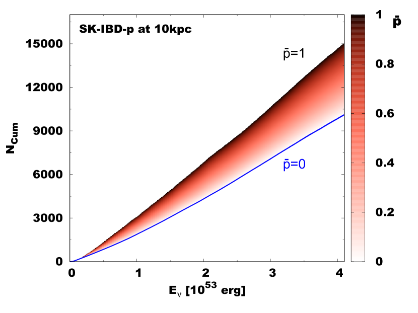
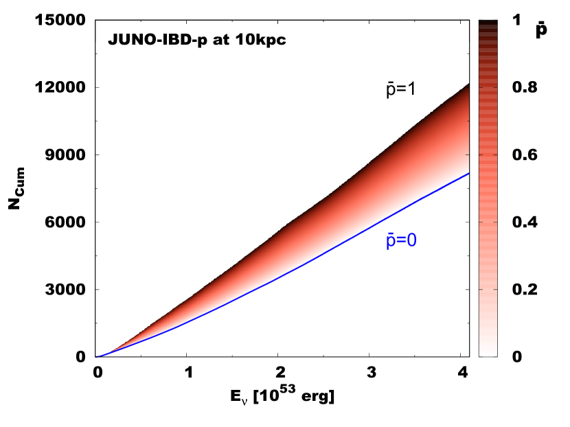
In Nagakura et al. (2021b, c); Vartanyan and Burrows (2023), we presented an in-depth analysis of neutrino signal from CCSNe and found that there is a robust correlation between the total neutrino energy (TONE or $E_{\nu}$) and the cumulative number of events ($N_{\rm Cum}$) in each detector. This correlation, however, depends on NFC model; for instance, $N_{\rm Cum}$ for a reaction channel by inverse-beta decay on protons (IBD-p), which corresponds to the major reaction for supernova neutrinos in Super-Kamiokande (SK) Abe and et al. (2016) and Jiangmen Underground Neutrino Observatory (JUNO) An et al. (2016), widely varies depending on the survival probability of neutrinos. To see the variation more quantitatively, we compute $N_{\rm Cum}$ by varying the survival probability of electron-type anti-neutrinos ($\bar{p}$) from 0 (maximum flavor conversion) to 1 (no flavor conversion) for the 20 M_⊙ progenitor in Burrows and Vartanyan (2021); Nagakura et al. (2021c), and the result is summarized in Fig. 1. As shown in this figure, determining $E_{\nu}$ from $N_{\rm Cum}$ has an uncertainty of $\sim 40\%$ due to $\bar{p}$.

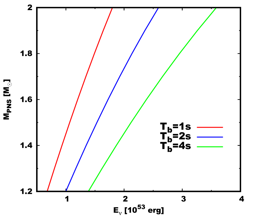
In our previous study Nagakura and Vartanyan (2022), we also found that PNS mass ($M_{\rm PNS}$) has a strong correlation with $E_{\nu}$. In the left panel of Fig. 2, we show $M_{\rm PNS}$ as a function of $E_{\nu}$ by using the result in Nagakura and Vartanyan (2022). We note that $E_{\nu}$ corresponds to the total emitted neutrino energy up to a certain post-bounce time ($T_{\rm b}$ which is measures from the time of core bounce), and we display three cases with $T_{\rm b}=1,2,$ and $4$s in the figure. To determine $T_{\rm b}$, we need to identify the core-bounce time in real observations, which is expected to be determined within the uncertainty of a few tens of milliseconds Halzen and Raffelt (2009). Since the uncertainty is much smaller than $T_{\rm b}$ which we consider ($>1$s), it does not affect our correlation study. One thing we need to mention here is, however, that the neutrino survival probability needs to be a priori set if we determine $M_{\rm PNS}$ from $N_{\rm Cum}$. This motivates the use of GW signal to remove the ambiguity of neutrino oscillation.

II.3 Gravitational waves

Let us turn our attention to GWs. The characteristic property of GWs in Fornax CCSN models have been studied in Morozova et al. (2018); Radice et al. (2019); Vartanyan et al. (2019); Vartanyan and Burrows (2020), and very recently Vartanyan et al. (2023) carried out a systematic study with long-term 3D simulations ($>1$s) and we quantify the total emitted energy of GWs ($E_{\rm GW}$). Although the high computational cost still limits the number of models, we find a robust correlation between $E_{\rm GW}$ and the compactness of the progenitor for explosion models. Observationally, this is useful, since $E_{\rm GW}$ may be the most easily constrained in real observations even for cases with no detections Abbott and et al. (2020). We note that $E_{\rm GW}$ is dominated by aspherical matter motions in the frequency range of $\gtrsim 100$ Hz, whereas the low frequency components including GW emission by anisotropic neutrino emission has a negligible contribution Mueller and Janka (1997); Abdikamalov et al. (2020); Vartanyan and Burrows (2020).

Let us describe the rationale behind the correlation between $E_{\rm GW}$ and the compactness of presupernova progenitor. The progenitor with the higher compactness core, in general, has higher mass accretion onto PNS in the post-bounce phase (see also Wang et al. (2022)), that also leads to heavier $M_{\rm PNS}$. Strong turbulent energy fluxes are accompanied by the large mass accretion onto PNS for explosion models, which is the major driving force emitting GWs. Here, we should make an important remark. The turbulence in post-shock region tends to be weak for non-exploding (or black hole formation) cases Vartanyan et al. (2023), since the accretion is more spherical and the post-shock accretion flow has higher temperature (i.e., low Mach number) than those in explosion models. This indicates that the correlation between $E_{\rm GW}$ and the compactness disappears in non-exploding models. For this reason, we adopt only explosion models in this correlation study. Although it is a limitation of the present work, the failure of explosion seems to be perhaps rarer than ordinary CCSNe Ugliano et al. (2012); Burrows and Vartanyan (2021); hence, our proposed method will be applied in the majority of the death of massive stars.

Figure 3: Flowchart of our proposed analysis. Red, blue, and green borders of each square distinguish observed quantities, theories, and output, respectively.

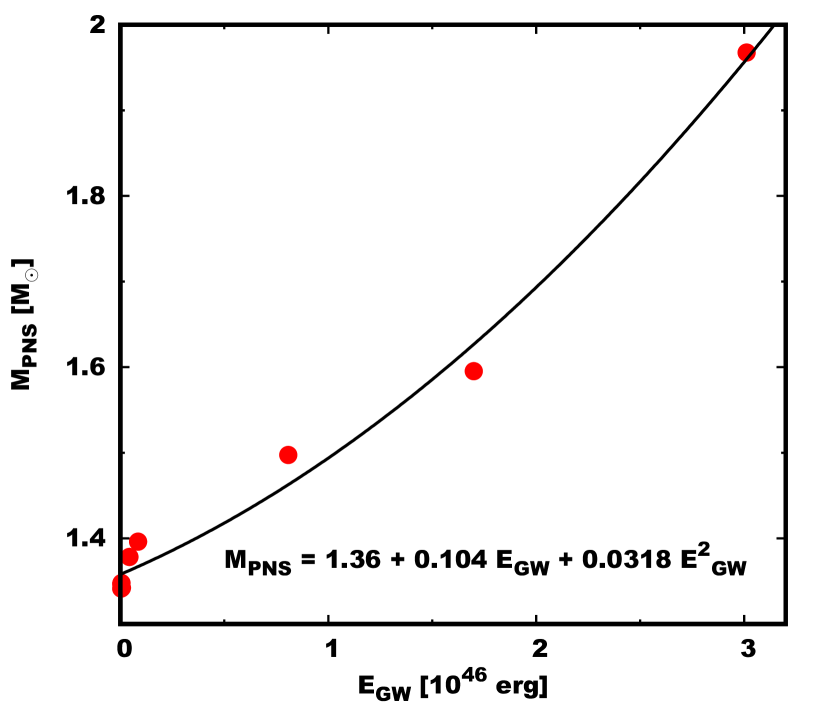
In the right panel of Fig. 2, we plot $M_{\rm PNS}$ (in the unit of solar mass, $M_{\odot}$) as a function of radiated GW energy ($E_{\rm GW}$ in the unit of $10^{46}{\rm erg}$) for 3D explosion models in Vartanyan et al. (2023). We note that GW strain is estimated by using the quadrupole approximation Finn and Evans (1990). The positive correlation can be clearly seen, and we show the quadratic fit as a black solid line in this figure. We note that the minimum mass of $M_{\rm PNS}$ obtained from the fitting function, $1.36M_{\odot}$, is not physical but rather an artifact due to the accuracy of polynominal fitting. The actual minimum PNS can be lower. We also quantify the coefficient of determination and standard deviation for the fitting function, which are $0.988$ and $0.018$, respectively. The latter is estimated based on a normalized error defined as $(M_{\rm PNS(d)}-M_{\rm PNS(f)})/M_{\rm PNS(f)}$, where $M_{\rm PNS(d)}$ and $M_{\rm PNS(f)}$ denote PNS mass at data point and that estimated by the fitting function, respectively.

II.4 Demonstration

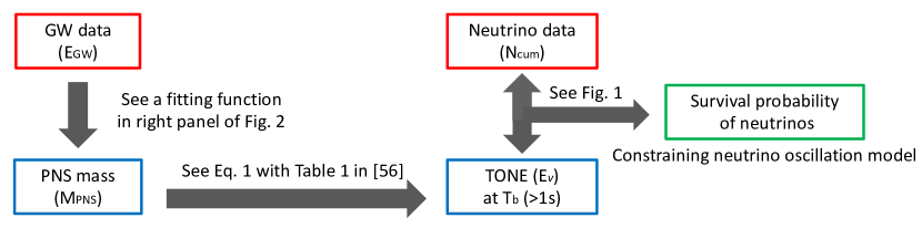
Below we describe how to place a constraint on $\bar{p}$ by using these three progenitor-independent correlations. We provide a flowchart of our proposed method in Fig. 3. For readers seeking more detailed understandings of our method, necessary references at each procedure are also described. As the first step, we need to set $T_{\rm b}$. According to Vartanyan et al. (2023), $E_{\rm GW}$ is mostly saturated up to $T_{\rm b}\sim 2$s, meanwhile the correlation of neutrino signal which we discussed in Nagakura et al. (2021c); Nagakura and Vartanyan (2022) is guaranteed up to $T_{\rm b}\sim 4$s; hence it should be set in the range of $2{\rm s}\lesssim T_{\rm b}\lesssim 4$s. Next, we estimate $M_{\rm PNS}$ from $E_{\rm GW}$ (see the right panel in Fig. 2), and then $E_{\nu}$ can be obtained from the correlation to $M_{\rm PNS}$ for given $T_{\rm b}$ (see the left panel in Fig. 2). $E_{\nu}$ provides the expected range of $N_{\rm Cum}$ depending on survival probability of neutrinos (see Fig. 1), and we can determine $\bar{p}$ by using the observed $N_{\rm Cum}$.

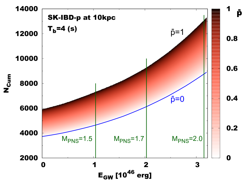
Fig. 4 depicts the summary of our proposed method. The color map displays $\bar{p}$ as a function of $E_{\rm GW}$ and $N_{\rm Cum}$ for a representative case of $T_{\rm b}=4$s. To guide the eye, the correspondence between $M_{\rm PNS}$ and $E_{\rm GW}$ can be seen as green vertical lines for three values of $M_{\rm PNS}$: $1.5,1.7,$ and $2.0M_{\odot}$. This clearly illustrates that $\bar{p}$ can be obtained from $T_{\rm b}$ and two observed quantities, $E_{\rm GW}$ and $N_{\rm Cum}$. We note that, in real observations, $E_{\rm GW}$ will be determined with errors, which depends on the signal-to-noise ratio (S/N). If $E_{\rm GW}$ is determined within the error of a few tens of percent, $\bar{p}$ can be constrained very well.

Finally, let us consider how we can use our proposed method in cases with no detection of GWs. We first need to estimate the distance to the CCSN source, which is expected to be given by neutrino and electro-magnetic signals (see also Sec. II.5 for more details). The obtained distance can be used to estimate the upper limit of $E_{\rm GW}$ (see, e.g., Abbott and et al. (2020)), that also provides the upper limit of $M_{\rm PNS}$ (see right panel of Fig. 2). On the other hand, the observed $N_{\rm Cum}$ gives another upper limit of $M_{\rm PNS}$ only through the correlation between $M_{\rm PNS}$ and neutrino signal. Our proposed method becomes very meaningful if the upper limit of $M_{\rm PNS}$ constrained by GW is smaller than that constrained by only the neutrino signal. In this case, $N_{\rm Cum}$ and the upper limit of $E_{GW}$ offers the lower limit of $\bar{p}$, i.e., narrowing down the possible $\bar{p}$ candidate. This is very informative to determine NFC in CCSN core.

Figure 4: $N_{\rm Cum}$ versus $E_{\rm GW}$. Color map and line types are the same as those used in Fig. 1. The vertical green lines at each panel highlight $M_{\rm PNS}=1.5,1.7,$ and $2.0M_{\odot}$, which is one-to-one relation with $E_{\rm GW}$ (see the left panel of Fig. 2). Left and right panels show the case with SK and JUNO, respectively for $T_{\rm b}=4$s.

II.5 Limitations

We add some important remarks in the present study. First, both detector- and Poisson noises in SK and JUNO do not compromise the estimation of $E_{\nu}$ from $N_{\rm Cum}$. Although the detector noise is a critical issue to retrieve energy spectrum of neutrinos from observed data Nagakura (2021), we only need energy-integrated number of events in our method, which is not affected by the detector noise. The Poisson noise of $N_{\rm Cum}$ is also very small (less than a few percent), since the total number of event counts is more than a few thousands for Galactic CCSNe. It should be mentioned, however, that neutrino detections by other channels, e.g., electron-scatterings, need to be separated for the precise determination of IBD-p events. The gadolinium (Gd) doping in water Cherenkov detector improves the neutron-tagging efficiency, which increases the accuracy of separation between IBD-p and electron-scattering events Beacom and Vagins (2004). Gd has already been loaded in SK, and SK-VI (the first SK-Gd project) operated from August 2020 to June 2022 with $5.4$ tons of gadolinium ($0.01\%$ mass concentration) Harada (2023) with a neutron capture efficiency of $\sim 50\%$. At the moment, SK-Gd is operating with $0.033\%$ mass concentration of Gd ($\sim 75\%$ neutron capture efficiency), and the SK-Gd project plans to increase the concentration up to $\sim 0.1\%$ in future, potentially offering $\sim 90\%$ neutron capture efficiency Hosokawa et al. (2023). Angular distributions of neutrino events also offer another means to distinguish IBD-p and electron-scattering. We can, hence, expect that IBD-p events will be identified well, although the quantitative discussion should be made in real observations.

Second, there is some degree of progenitor dependence in the correlation between $E_{\nu}$ and $N_{\rm Cum}$, which is $\lesssim 10\%$ for IBD-p events in SK and JUNO (see Fig.14 in Nagakura et al. (2021c)). The progenitor dependence tends to be remarkable in the case with no flavor conversion (i.e., $\bar{p}=1$), whereas it monotonically decreases with $\bar{p}\to 0$. This is attributed to the two reasons. The first one is that IBD-p becomes sensitive to heavy-leptonic neutrinos at the CCSN source, which dominates the irradiated energy of neutrinos. This enhances the correlation between $E_{\nu}$ and $N_{\rm Cum}$. The other reason is that neutrino luminosity of heavy-leptonic neutrinos is dominated by the diffusion component, while the accretion component plays a non-negligible role in electron-type neutrinos and antineutrinos. The accretion component depends on the density profile of progenitor, indicating that the progenitor dependence tends to be stronger. Since the case with no flavor conversion, $N_{\rm Cum}$ is determined only by electron-type neutrinos at the source, leading to relatively larger progenitor dependence. This consideration suggests that, if $\bar{p}=1$ is obtained in real data analysis, we need to keep in mind the progenitor-dependent uncertainty.

Third, $N_{\rm Cum}$ in general depends on the observer direction, and the angular variation of the time-integrated event rate would be more than $10\%$ for some CCSNe Vartanyan et al. (2019); Nagakura et al. (2021b). This indicates that the uncertainty of observer location potentially becomes a major systematic error in our proposed method. It is worth to note, however, that the asymmetry of neutrino emission can be estimated if low frequency (below $\sim 10$ Hz) GWs are detected. This is because the so-called memory effect of neutrino emision seems to dominate GWs in these frequency range Braginskii and Thorne (1987); Mueller and Janka (1997); Kotake et al. (2007, 2009); Müller et al. (2012); Vartanyan and Burrows (2020); Fu and Yamada (2022). This indicates that the multi-band GW analysis offers valuable information for our proposed method. In fact, it is impossible to constrain the asymmetry of neutrino emission only by neutrino observations.

Fourth, precise estimations of $E_{\nu}$ and $E_{\rm GW}$ require accurate determinations of distance to the CCSN source. The distance may be constrained by the neutronization burst within the error of $\sim 5\%$ Kachelrieß et al. (2005). Electro-magnetic wave (EM) observations can also provide another independent measurement; for instance, the angular diameter distance can be estimated from the angular size of the ejecta and its spatial size. The former is given by observations, and the latter is estimated by two quantities: the time since the explosion and the expansion veloity of the ejecta deduced from theoretical considerations. We also note that the pre-explosion image of CCSN progenitor may be available in the catalog of nearby red supergiants. This observation also offers the distance information independently from others. Although the precision of the measurement hinges on the CCSN event, the cross-check among these independent measuremets will reduce the distance uncertainty.

Fifth, one has to keep in mind another caveat in the present study. $\bar{p}$ is assumed to be constant in time when we quantify the correlation between $E_{\nu}$ from $N_{\rm Cum}$. However, $\bar{p}$ is in general time-dependent. This indicates that our proposed method has the ability to constrain only the time-averaged $\bar{p}$, and that systematic errors may become large if $\bar{p}$ varies with time considerably. The maximum error is quantified in principle by changing $\bar{p}$ as a function of time in our correlation study. We leave this problem for the future.

Sixth, we summarize potential systematic errors inherent in our CCSN models. The sensitivity to input physics (EOS and neutrino-matter interactions) to the correlation remains uncertain; indeed, we focused only the SFHo EOS and neutrino-matter interactions in our CCSN models, that would affect the correlations quantitatively. As another caveat, rotation may be an important contributor to GW and neutrino signals. However, our correlation study is made for non-rotating progenitors. We also note that CCSN models may have endemic unknown systematic errors due to complex numerical implementations of input physics.

Finally, we discuss how these systematic uncertainties and errors in observed quantities affect constraints on $\bar{p}$, which provides the range of application for our proposed method. As displayed in Fig. 4, $\sim 30\%$ error in $N_{\rm Cum}$ overwhelms the variation by $\bar{p}$. This indicates that other potential uncertainties (e.g., distance error, angular variations, progenitor dependences, and systematic errors in CCSN models) become a critical problem in our proposed method, if they lead to the same amount of uncertainty in $N_{\rm Cum}$. For similar reasons, the error in $E_{\rm GW}$ (and an associated uncertainty in the correlation between $E_{\rm GW}$ and $M_{\rm PNS}$) needs to be within $\sim 40\%$ to place a constraint on $\bar{p}$. As already pointed out, however, the upper limit of $E_{\rm GW}$ is still meaningful even if GWs are not observed.

Last but not least, it is very important to carry out a similar correlation study based on models simulated by different CCSN groups so as to reduce the systematic uncertainties in our proposed method. The survival probability of neutrinos and PNS mass will be estimated independently in each group, and then they will be compared among different groups. Such a collaborative work is indispensable to quantify the theoretical uncertainty, and it also increases statistics in the correlation analysis. We leave all these detailed investigations and fruitful collaborations as future work.

III Summary

In this paper, we propose a new approach of GW-neutrino joint analysis for CCSNe, based on the correlation study of most recent multi-D CCSN explosion models. Our method is designed so as to determine the survival probability of neutrinos and PNS mass, which are both key ingredients to characterize CCSN dynamics. One of the useful features in the proposed method is that we can apply it even in cases with no detection of GWs. This is a great advantage compared to other proposed GW-neutrino analysis, for instance GW spectrogram analysis Kuroda et al. (2016); Andresen et al. (2017); Radice et al. (2019); Mezzacappa et al. (2020); Jakobus et al. (2023); Fuller et al. (2015); Sotani et al. (2017); Torres-Forné et al. (2018); Morozova et al. (2018); Torres-Forné et al. (2019a, b); Bizouard et al. (2021); Bruel et al. (2023), that commonly requires GW data with high S/N.

Finally, we put a comment on how EM signal can complement the proposed method. In recent CCSN simulations, a positive correlation between PNS mass and explosion energy of CCSNe can be seen, albeit somewhat weaker correlations than GWs and neutrinos. According to Wang et al. (2022), the explosion energy can reach $>10^{51}{\rm erg}$ only if $M_{\rm PNS}$ is larger than $\sim 1.7M_{\odot}$. This exhibits that the EM observations offer an independent constraint on $M_{\rm PNS}$, and they can be used as a consistency check to that obtained from the present method. As such, there is surely room for improvements, but this study offers a feasible way for multi-messenger analyses with numerical CCSN models.

IV DATA AVAILABILITY

The data underlying this article will be shared on reasonable request to the corresponding author.

V Acknowledgments

We are grateful for ongoing contributions to the effort of CCSN simulation projects by Adam Burrows, David Radice, Josh Dolence, Aaron Skinner, Matthew Coleman, Chris White, and Tianshu Wang. HN is supported by Grant-inAid for Scientific Research (23K03468). DV acknowledges support from the NASA Hubble Fellowship Program grant HST-HF2-51520.

References

- Abdikamalov et al. (2020) Ernazar Abdikamalov, Giulia Pagliaroli, and David Radice, “Gravitational Waves from Core-Collapse Supernovae,” arXiv e-prints , arXiv:2010.04356 (2020), arXiv:2010.04356 [astro-ph.SR] .
- Mirizzi et al. (2016) A. Mirizzi, I. Tamborra, H. Th. Janka, N. Saviano, K. Scholberg, R. Bollig, L. Hüdepohl, and S. Chakraborty, “Supernova neutrinos: production, oscillations and detection,” Nuovo Cimento Rivista Serie 39, 1–112 (2016), arXiv:1508.00785 [astro-ph.HE] .
- Horiuchi and Kneller (2018) Shunsaku Horiuchi and James P. Kneller, “What can be learned from a future supernova neutrino detection?” Journal of Physics G Nuclear Physics 45, 043002 (2018), arXiv:1709.01515 [astro-ph.HE] .
- Müller (2019) B. Müller, “Neutrino Emission as Diagnostics of Core-Collapse Supernovae,” Annual Review of Nuclear and Particle Science 69, 253–278 (2019), arXiv:1904.11067 [astro-ph.HE] .
- Kuroda et al. (2016) Takami Kuroda, Kei Kotake, and Tomoya Takiwaki, “A New Gravitational-wave Signature from Standing Accretion Shock Instability in Supernovae,” ApJ 829, L14 (2016).
- Andresen et al. (2017) H. Andresen, B. Müller, E. Müller, and H. Th. Janka, “Gravitational wave signals from 3D neutrino hydrodynamics simulations of core-collapse supernovae,” MNRAS 468, 2032–2051 (2017).
- Radice et al. (2019) David Radice, Viktoriya Morozova, Adam Burrows, David Vartanyan, and Hiroki Nagakura, “Characterizing the Gravitational Wave Signal from Core-collapse Supernovae,” ApJ 876, L9 (2019), arXiv:1812.07703 [astro-ph.HE] .
- Mezzacappa et al. (2020) Anthony Mezzacappa, Pedro Marronetti, Ryan E. Landfield, Eric J. Lentz, Konstantin N. Yakunin, Stephen W. Bruenn, W. Raphael Hix, O. E. Bronson Messer, Eirik Endeve, John M. Blondin, and J. Austin Harris, “Gravitational-wave signal of a core-collapse supernova explosion of a 15 M star,” Phys. Rev. D 102, 023027 (2020), arXiv:2007.15099 [astro-ph.HE] .
- Jakobus et al. (2023) Pia Jakobus, Bernhard Müller, Alexander Heger, Shuai Zha, Jade Powell, Anton Motornenko, Jan Steinheimer, and Horst Stoecker, “Gravitational Waves from a Core g-Mode in Supernovae as Probes of the High-Density Equation of State,” arXiv e-prints , arXiv:2301.06515 (2023), arXiv:2301.06515 [astro-ph.HE] .
- Fuller et al. (2015) Jim Fuller, Hannah Klion, Ernazar Abdikamalov, and Christian D. Ott, “Supernova seismology: gravitational wave signatures of rapidly rotating core collapse,” MNRAS 450, 414–427 (2015), arXiv:1501.06951 [astro-ph.HE] .
- Sotani et al. (2017) Hajime Sotani, Takami Kuroda, Tomoya Takiwaki, and Kei Kotake, “Probing mass-radius relation of protoneutron stars from gravitational-wave asteroseismology,” Phys. Rev. D 96, 063005 (2017), arXiv:1708.03738 [astro-ph.HE] .
- Torres-Forné et al. (2018) Alejandro Torres-Forné, Pablo Cerdá-Durán, Andrea Passamonti, and José A. Font, “Towards asteroseismology of core-collapse supernovae with gravitational-wave observations - I. Cowling approximation,” MNRAS 474, 5272–5286 (2018), arXiv:1708.01920 [astro-ph.SR] .
- Morozova et al. (2018) V. Morozova, D. Radice, A. Burrows, and D. Vartanyan, “The Gravitational Wave Signal from Core-collapse Supernovae,” ApJ 861, 10 (2018), arXiv:1801.01914 [astro-ph.HE] .
- Torres-Forné et al. (2019a) Alejandro Torres-Forné, Pablo Cerdá-Durán, Andrea Passamonti, Martin Obergaulinger, and José A. Font, “Towards asteroseismology of core-collapse supernovae with gravitational wave observations - II. Inclusion of space-time perturbations,” MNRAS 482, 3967–3988 (2019a), arXiv:1806.11366 [astro-ph.HE] .
- Torres-Forné et al. (2019b) Alejandro Torres-Forné, Pablo Cerdá-Durán, Martin Obergaulinger, Bernhard Müller, and José A. Font, “Universal Relations for Gravitational-Wave Asteroseismology of Protoneutron Stars,” Phys. Rev. Lett. 123, 051102 (2019b), arXiv:1902.10048 [gr-qc] .
- Bizouard et al. (2021) Marie-Anne Bizouard, Patricio Maturana-Russel, Alejandro Torres-Forné, Martin Obergaulinger, Pablo Cerdá-Durán, Nelson Christensen, José A. Font, and Renate Meyer, “Inference of protoneutron star properties from gravitational-wave data in core-collapse supernovae,” Phys. Rev. D 103, 063006 (2021), arXiv:2012.00846 [gr-qc] .
- Bruel et al. (2023) Tristan Bruel, Marie-Anne Bizouard, Martin Obergaulinger, Patricio Maturana-Russel, Alejandro Torres-Forné, Pablo Cerdá-Durán, Nelson Christensen, José A. Font, and Renate Meyer, “Inference of protoneutron star properties in core-collapse supernovae from a gravitational-wave detector network,” Phys. Rev. D 107, 083029 (2023), arXiv:2301.10019 [astro-ph.HE] .
- Nakamura et al. (2016) Ko Nakamura, Shunsaku Horiuchi, Masaomi Tanaka, Kazuhiro Hayama, Tomoya Takiwaki, and Kei Kotake, “Multimessenger signals of long-term core-collapse supernova simulations: synergetic observation strategies,” MNRAS 461, 3296–3313 (2016), arXiv:1602.03028 [astro-ph.HE] .
- Kuroda et al. (2017) Takami Kuroda, Kei Kotake, Kazuhiro Hayama, and Tomoya Takiwaki, “Correlated Signatures of Gravitational-wave and Neutrino Emission in Three-dimensional General-relativistic Core-collapse Supernova Simulations,” ApJ 851, 62 (2017), arXiv:1708.05252 [astro-ph.HE] .
- Warren et al. (2020) MacKenzie L. Warren, Sean M. Couch, Evan P. O’Connor, and Viktoriya Morozova, “Constraining Properties of the Next Nearby Core-collapse Supernova with Multimessenger Signals,” ApJ 898, 139 (2020), arXiv:1912.03328 [astro-ph.HE] .
- Szczepańczyk et al. (2021) Marek J. Szczepańczyk, Javier M. Antelis, Michael Benjamin, Marco Cavaglià, Dorota Gondek-Rosińska, Travis Hansen, Sergey Klimenko, Manuel D. Morales, Claudia Moreno, Soma Mukherjee, Gaukhar Nurbek, Jade Powell, Neha Singh, Satzhan Sitmukhambetov, Paweł Szewczyk, Oscar Valdez, Gabriele Vedovato, Jonathan Westhouse, Michele Zanolin, and Yanyan Zheng, “Detecting and reconstructing gravitational waves from the next galactic core-collapse supernova in the advanced detector era,” Phys. Rev. D 104, 102002 (2021), arXiv:2104.06462 [astro-ph.HE] .
- Drago et al. (2023) Marco Drago, Haakon Andresen, Irene Di Palma, Irene Tamborra, and Alejandro Torres-Forné, “Multi-messenger observations of core-collapse supernovae: Exploiting the standing accretion shock instability,” arXiv e-prints , arXiv:2305.07688 (2023), arXiv:2305.07688 [astro-ph.HE] .
- Abbott and et al. (2020) B. P. Abbott and et al., “Optically targeted search for gravitational waves emitted by core-collapse supernovae during the first and second observing runs of advanced LIGO and advanced Virgo,” Phys. Rev. D 101, 084002 (2020), arXiv:1908.03584 [astro-ph.HE] .
- Powell and Müller (2020) Jade Powell and Bernhard Müller, “Three-dimensional core-collapse supernova simulations of massive and rotating progenitors,” MNRAS 494, 4665–4675 (2020), arXiv:2002.10115 [astro-ph.HE] .
- Mezzacappa et al. (2023) Anthony Mezzacappa, Pedro Marronetti, Ryan E. Landfield, Eric J. Lentz, R. Daniel Murphy, W. Raphael Hix, J. Austin Harris, Stephen W. Bruenn, John M. Blondin, O. E. Bronson Messer, Jordi Casanova, and Luke L. Kronzer, “Core collapse supernova gravitational wave emission for progenitors of 9.6, 15, and 25 M⊙,” Phys. Rev. D 107, 043008 (2023), arXiv:2208.10643 [astro-ph.SR] .
- Dighe and Smirnov (2000) Amol S. Dighe and Alexei Yu. Smirnov, “Identifying the neutrino mass spectrum from a supernova neutrino burst,” Phys. Rev. D 62, 033007 (2000), arXiv:hep-ph/9907423 [hep-ph] .
- Chakraborty et al. (2016) Sovan Chakraborty, Rasmus Hansen, Ignacio Izaguirre, and Georg Raffelt, “Collective neutrino flavor conversion: Recent developments,” Nuclear Physics B 908, 366–381 (2016), arXiv:1602.02766 [hep-ph] .
- Tamborra and Shalgar (2021) Irene Tamborra and Shashank Shalgar, “New Developments in Flavor Evolution of a Dense Neutrino Gas,” Annual Review of Nuclear and Particle Science 71, 165–188 (2021), arXiv:2011.01948 [astro-ph.HE] .
- Capozzi and Saviano (2022) Francesco Capozzi and Ninetta Saviano, “Neutrino Flavor Conversions in High-Density Astrophysical and Cosmological Environments,” Universe 8, 94 (2022), arXiv:2202.02494 [hep-ph] .
- Richers and Sen (2022) Sherwood Richers and Manibrata Sen, “Fast Flavor Transformations,” arXiv e-prints , arXiv:2207.03561 (2022), arXiv:2207.03561 [astro-ph.HE] .
- Nagakura et al. (2019) Hiroki Nagakura, Taiki Morinaga, Chinami Kato, and Shoichi Yamada, “Fast-pairwise Collective Neutrino Oscillations Associated with Asymmetric Neutrino Emissions in Core-collapse Supernovae,” ApJ 886, 139 (2019), arXiv:1910.04288 [astro-ph.HE] .
- Shalgar and Tamborra (2019) Shashank Shalgar and Irene Tamborra, “On the Occurrence of Crossings between the Angular Distributions of Electron Neutrinos and Antineutrinos in the Supernova Core,” ApJ 883, 80 (2019), arXiv:1904.07236 [astro-ph.HE] .
- Delfan Azari et al. (2020) Milad Delfan Azari, Shoichi Yamada, Taiki Morinaga, Hiroki Nagakura, Shun Furusawa, Akira Harada, Hirotada Okawa, Wakana Iwakami, and Kohsuke Sumiyoshi, “Fast collective neutrino oscillations inside the neutrino sphere in core-collapse supernovae,” Phys. Rev. D 101, 023018 (2020), arXiv:1910.06176 [astro-ph.HE] .
- Morinaga et al. (2020) Taiki Morinaga, Hiroki Nagakura, Chinami Kato, and Shoichi Yamada, “Fast neutrino-flavor conversion in the preshock region of core-collapse supernovae,” Physical Review Research 2, 012046 (2020), arXiv:1909.13131 [astro-ph.HE] .
- Nagakura et al. (2021a) Hiroki Nagakura, Adam Burrows, Lucas Johns, and George M. Fuller, “Where, when, and why: Occurrence of fast-pairwise collective neutrino oscillation in three-dimensional core-collapse supernova models,” Phys. Rev. D 104, 083025 (2021a), arXiv:2108.07281 [astro-ph.HE] .
- Abbar et al. (2021) Sajad Abbar, Francesco Capozzi, Robert Glas, H. Thomas Janka, and Irene Tamborra, “On the characteristics of fast neutrino flavor instabilities in three-dimensional core-collapse supernova models,” Phys. Rev. D 103, 063033 (2021), arXiv:2012.06594 [astro-ph.HE] .
- Capozzi et al. (2021) Francesco Capozzi, Sajad Abbar, Robert Bollig, and H. Thomas Janka, “Fast neutrino flavor conversions in one-dimensional core-collapse supernova models with and without muon creation,” Phys. Rev. D 103, 063013 (2021), arXiv:2012.08525 [astro-ph.HE] .
- Harada and Nagakura (2022) Akira Harada and Hiroki Nagakura, “Prospects of Fast Flavor Neutrino Conversion in Rotating Core-collapse Supernovae,” ApJ 924, 109 (2022), arXiv:2110.08291 [astro-ph.HE] .
- Xiong et al. (2023) Zewei Xiong, Meng-Ru Wu, Gabriel Martínez-Pinedo, Tobias Fischer, Manu George, Chun-Yu Lin, and Lucas Johns, “Evolution of collisional neutrino flavor instabilities in spherically symmetric supernova models,” Phys. Rev. D 107, 083016 (2023), arXiv:2210.08254 [astro-ph.HE] .
- Nagakura (2023) Hiroki Nagakura, “Roles of Fast Neutrino-Flavor Conversion on the Neutrino-Heating Mechanism of Core-Collapse Supernova,” Phys. Rev. Lett. 130, 211401 (2023), arXiv:2301.10785 [astro-ph.HE] .
- Nagakura et al. (2021b) Hiroki Nagakura, Adam Burrows, David Vartanyan, and David Radice, “Core-collapse supernova neutrino emission and detection informed by state-of-the-art three-dimensional numerical models,” MNRAS 500, 696–717 (2021b), arXiv:2007.05000 [astro-ph.HE] .
- Nagakura et al. (2021c) Hiroki Nagakura, Adam Burrows, and David Vartanyan, “Supernova neutrino signals based on long-term axisymmetric simulations,” MNRAS 506, 1462–1479 (2021c), arXiv:2102.11283 [astro-ph.HE] .
- Eggenberger Andersen et al. (2021) Oliver Eggenberger Andersen, Shuai Zha, André da Silva Schneider, Aurore Betranhandy, Sean M. Couch, and Evan P. O’Connor, “Equation-of-state Dependence of Gravitational Waves in Core-collapse Supernovae,” ApJ 923, 201 (2021), arXiv:2106.09734 [astro-ph.HE] .
- Vartanyan et al. (2023) David Vartanyan, Adam Burrows, Tianshu Wang, Matthew S. B. Coleman, and Christopher J. White, “Gravitational-wave signature of core-collapse supernovae,” Phys. Rev. D 107, 103015 (2023), arXiv:2302.07092 [astro-ph.HE] .
- Skinner et al. (2019) M. Aaron Skinner, Joshua C. Dolence, Adam Burrows, David Radice, and David Vartanyan, “FORNAX: A Flexible Code for Multiphysics Astrophysical Simulations,” The Astrophysical Journal Supplement Series 241, 7 (2019), arXiv:1806.07390 [astro-ph.IM] .
- Burrows et al. (2020) Adam Burrows, David Radice, David Vartanyan, Hiroki Nagakura, M. Aaron Skinner, and Joshua C. Dolence, “The overarching framework of core-collapse supernova explosions as revealed by 3D FORNAX simulations,” MNRAS 491, 2715–2735 (2020), arXiv:1909.04152 [astro-ph.HE] .
- Burrows and Vartanyan (2021) A. Burrows and D. Vartanyan, “Core-collapse supernova explosion theory,” Nature 589, 29–39 (2021), arXiv:2009.14157 [astro-ph.SR] .
- Vaytet et al. (2011) N. M. H. Vaytet, E. Audit, B. Dubroca, and F. Delahaye, “A numerical model for multigroup radiation hydrodynamics,” Journal of Quantitative Spectroscopy and Radiative Transfer 112, 1323–1335 (2011), arXiv:1101.4955 [astro-ph.HE] .
- Steiner et al. (2013) A. W. Steiner, M. Hempel, and T. Fischer, “Core-collapse Supernova Equations of State Based on Neutron Star Observations,” ApJ 774, 17 (2013), arXiv:1207.2184 [astro-ph.SR] .
- Burrows et al. (2006) A. Burrows, S. Reddy, and T. A. Thompson, “Neutrino opacities in nuclear matter,” Nuclear Physics A 777, 356–394 (2006), astro-ph/0404432 .
- Horowitz et al. (2017) C. J. Horowitz, O. L. Caballero, Z. Lin, E. O’Connor, and A. Schwenk, “Neutrino-nucleon scattering in supernova matter from the virial expansion,” Phys. Rev. C 95, 025801 (2017), arXiv:1611.05140 [nucl-th] .
- Juodagalvis et al. (2010) A. Juodagalvis, K. Langanke, W. R. Hix, G. Martínez-Pinedo, and J. M. Sampaio, “Improved estimate of electron capture rates on nuclei during stellar core collapse,” Nuclear Physics A 848, 454–478 (2010), arXiv:0909.0179 [nucl-th] .
- Vartanyan and Burrows (2023) David Vartanyan and Adam Burrows, “Neutrino Signatures of One Hundred 2D Axisymmetric Core-Collapse Supernova Simulations,” arXiv e-prints , arXiv:2307.08735 (2023), arXiv:2307.08735 [astro-ph.HE] .
- Abe and et al. (2016) K. Abe and et al., “Real-time supernova neutrino burst monitor at Super-Kamiokande,” Astroparticle Physics 81, 39–48 (2016), arXiv:1601.04778 [astro-ph.HE] .
- An et al. (2016) Fengpeng An, Guangpeng An, Qi An, Vito Antonelli, Eric Baussan, John Beacom, Leonid Bezrukov, Simon Blyth, Riccardo Brugnera, Margherita Buizza Avanzini, and et al., “Neutrino physics with JUNO,” Journal of Physics G Nuclear Physics 43, 030401 (2016), arXiv:1507.05613 [physics.ins-det] .
- Nagakura and Vartanyan (2022) Hiroki Nagakura and David Vartanyan, “Efficient method for estimating the time evolution of the proto-neutron star mass and radius from a supernova neutrino signal,” MNRAS 512, 2806–2816 (2022), arXiv:2111.05869 [astro-ph.HE] .
- Halzen and Raffelt (2009) Francis Halzen and Georg G. Raffelt, “Reconstructing the supernova bounce time with neutrinos in IceCube,” Phys. Rev. D 80, 087301 (2009), arXiv:0908.2317 [astro-ph.HE] .
- Vartanyan et al. (2019) David Vartanyan, Adam Burrows, and David Radice, “Temporal and angular variations of 3D core-collapse supernova emissions and their physical correlations,” MNRAS 489, 2227–2246 (2019), arXiv:1906.08787 [astro-ph.HE] .
- Vartanyan and Burrows (2020) David Vartanyan and Adam Burrows, “Gravitational Waves from Neutrino Emission Asymmetries in Core-collapse Supernovae,” ApJ 901, 108 (2020), arXiv:2007.07261 [astro-ph.HE] .
- Mueller and Janka (1997) E. Mueller and H. T. Janka, “Gravitational radiation from convective instabilities in Type II supernova explosions.” A&A 317, 140–163 (1997).
- Wang et al. (2022) Tianshu Wang, David Vartanyan, Adam Burrows, and Matthew S. B. Coleman, “The essential character of the neutrino mechanism of core-collapse supernova explosions,” MNRAS 517, 543–559 (2022), arXiv:2207.02231 [astro-ph.SR] .
- Ugliano et al. (2012) Marcella Ugliano, Hans-Thomas Janka, Andreas Marek, and Almudena Arcones, “Progenitor-explosion Connection and Remnant Birth Masses for Neutrino-driven Supernovae of Iron-core Progenitors,” ApJ 757, 69 (2012), arXiv:1205.3657 [astro-ph.SR] .
- Finn and Evans (1990) Lee Samuel Finn and Charles R. Evans, “Determing gravitational radiation from Newtonian self-gravitating systems.” ApJ 351, 588–600 (1990).
- Nagakura (2021) Hiroki Nagakura, “Retrieval of energy spectra for all flavours of neutrinos from core-collapse supernova with multiple detectors,” MNRAS 500, 319–332 (2021), arXiv:2008.10082 [astro-ph.HE] .
- Beacom and Vagins (2004) John F. Beacom and Mark R. Vagins, “Antineutrino Spectroscopy with Large Water Čerenkov Detectors,” Phys. Rev. Lett. 93, 171101 (2004), arXiv:hep-ph/0309300 [hep-ph] .
- Harada (2023) M. et al. Harada, “Search for astrophysical electron antineutrinos in Super-Kamiokande with 0.01wt% gadolinium-loaded water,” arXiv e-prints , arXiv:2305.05135 (2023), arXiv:2305.05135 [astro-ph.HE] .
- Hosokawa et al. (2023) K. Hosokawa, M. Ikeda, T. Okada, H. Sekiya, P. Fernández, L. Labarga, I. Bandac, J. Perez, S. Ito, M. Harada, Y. Koshio, M. D. Thiesse, L. F. Thompson, P. R. Scovell, E. Meehan, K. Ichimura, Y. Kishimoto, Y. Nakajima, M. R. Vagins, H. Ito, Y. Takaku, Y. Tanaka, and Y. Yamaguchi, “Development of ultra-pure gadolinium sulfate for the Super-Kamiokande gadolinium project,” Progress of Theoretical and Experimental Physics 2023, 013H01 (2023), arXiv:2209.07273 [physics.ins-det] .
- Braginskii and Thorne (1987) V. B. Braginskii and Kip S. Thorne, “Gravitational-wave bursts with memory and experimental prospects,” Nature 327, 123–125 (1987).
- Kotake et al. (2007) Kei Kotake, Naofumi Ohnishi, and Shoichi Yamada, “Gravitational Radiation from Standing Accretion Shock Instability in Core-Collapse Supernovae,” ApJ 655, 406–415 (2007), arXiv:astro-ph/0607224 [astro-ph] .
- Kotake et al. (2009) Kei Kotake, Wakana Iwakami, Naofumi Ohnishi, and Shoichi Yamada, “Stochastic Nature of Gravitational Waves from Supernova Explosions with Standing Accretion Shock Instability,” ApJ 697, L133–L136 (2009), arXiv:0904.4300 [astro-ph.HE] .
- Müller et al. (2012) E. Müller, H. Th. Janka, and A. Wongwathanarat, “Parametrized 3D models of neutrino-driven supernova explosions. Neutrino emission asymmetries and gravitational-wave signals,” A&A 537, A63 (2012), arXiv:1106.6301 [astro-ph.SR] .
- Fu and Yamada (2022) Lei Fu and Shoichi Yamada, “Gravitational wave signals in the deci-Hz range from neutrinos during the protoneutron star cooling phase,” Phys. Rev. D 105, 123028 (2022), arXiv:2201.12774 [astro-ph.HE] .
- Kachelrieß et al. (2005) M. Kachelrieß, R. Tomàs, R. Buras, H.-T. Janka, A. Marek, and M. Rampp, “Exploiting the neutronization burst of a galactic supernova,” Phys. Rev. D 71, 063003 (2005), astro-ph/0412082 .