PanoSwin: a Pano-style Swin Transformer for Panorama Understanding

Abstract

In panorama understanding, the widely used equirectangular projection (ERP) entails boundary discontinuity and spatial distortion. It severely deteriorates the conventional CNNs and vision Transformers on panoramas. In this paper, we propose a simple yet effective architecture named PanoSwin to learn panorama representations with ERP. To deal with the challenges brought by equirectangular projection, we explore a pano-style shift windowing scheme and novel pitch attention to address the boundary discontinuity and the spatial distortion, respectively. Besides, based on spherical distance and Cartesian coordinates, we adapt absolute positional embeddings and relative positional biases for panoramas to enhance panoramic geometry information. Realizing that planar image understanding might share some common knowledge with panorama understanding, we devise a novel two-stage learning framework to facilitate knowledge transfer from the planar images to panoramas. We conduct experiments against the state-of-the-art on various panoramic tasks, i.e., panoramic object detection, panoramic classification, and panoramic layout estimation. The experimental results demonstrate the effectiveness of PanoSwin in panorama understanding.

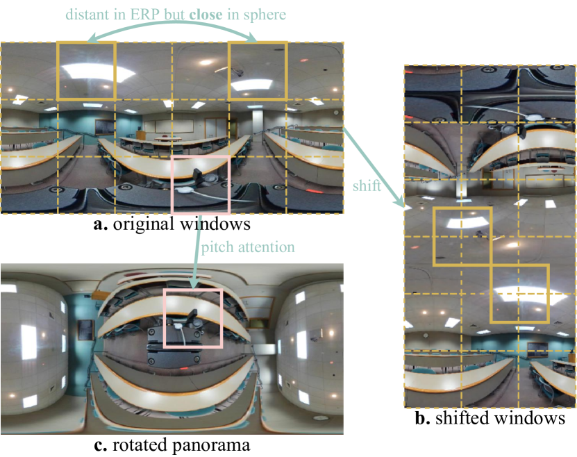
Figure 1: (1). Fig. a is how a panoramic image looks, just like a planar world map, where top/bottom regions are connected to the earth’s poles; the right side is connected to the left. (2). Our PanoSwin is based on window attention[21]. Fig. a also shows the original window partition in dotted orange, where the two windows in bold orange are separated by equirectangular projection(ERP). (3). Fig. b shows pano-style shift windowing scheme, which brings the two departed regions together. (4). Fig. c shows our pitch attention module, which helps a distorted window to interact with an undistorted one.

1 Introduction

Panoramas are widely used in many real applications, such as virtual reality, autonomous driving, civil surveillance, etc. Panorama understanding has attracted increasing interest in the research community [38, 5, 29]. Among these methods, the most popular and convenient representation of panorama is adopted via equirectangular projection (ERP), which maps the latitude and longitude of the spherical representation to horizontal and vertical grid coordinates. However, the inherent omnidirectional vision remains the challenge of the panorama understanding. Although convolutional neural networks (CNNs)[11, 30, 14] have shown outstanding performances on planar image understanding, most CNN-based methods are unsuitable for panoramas because of two fundamental problems entailed by ERP: (1) polar and side boundary discontinuity and (2) spatial distortion. Specifically, the north/south polar region in spherical representations are closely connected. But the converted region covers the whole top/bottom boundaries. On this account, polar boundary continuity is destroyed by ERP. Similarly, side boundary continuity is also destroyed since the left and right sides are split by ERP. Meanwhile, spatial distortion also severely deforms the image content, especially in polar regions.

A common solution is to adapt convolution to the spherical space[38, 5, 26, 4]. However, these methods might suffer from high computation costs from the adaptation process. Besides, Spherical Transformer[2] and PanoFormer[24] specially devise patch sampling approaches to remove panoramic distortion. However, the specially designed patch sampling approaches might not be feasible for planar images. In our experiments, we demonstrate that exploiting planar knowledge can boost the performance of panorama understanding.

Inspired by Swin Transformer[21], we propose PanoSwin Transformer to reduce the distortion of panoramic images, as briefly shown in Fig. 1. To cope with boundary discontinuity, we explore a pano-style shift windowing scheme (PSW). In PSW, side continuity is established by horizontal shift. To establish polar continuity, we first split the panorama in half and then rotate the right half counterclockwise. To overcome spatial distortion, we first rotate the pitch of the panorama by $0.5\pi$. So the polar regions of the original feature map are “swapped” with some equator regions of the rotated panorama. For each window in the original panorama, we locate a corresponding window in the rotated panorama. Then we perform cross-attention between these two windows. We name the module pitch attention (PA), which is plug-and-play and can be inserted in various backbones. Intuitively, pitch attention can help a window “know” how it looks without distortion.

To leverage planar knowledge, some works[27, 26] proposed to make novel panoramic kernel mimick outputs from planar convolution kernel layer by layer. However, PanoSwin is elaborately designed to be compatible with planar images: PanoSwin can be switched from pano mode to vanilla swin mode. Let PanoSwin in these two modes be denoted as PanoSwin_p and PanoSwin_s. PanoSwin_p/PanoSwin_s can be adopted to process panoramas/planar images, details about which will be introduced in Sec. 3.6. In our paper, PanoSwin is under pano mode by default. The double-mode feature of PanoSwin makes it possible to devise a simple two-stage learning paradigm based on knowledge preservation to leverage planar knowledge: we first pretrain PanoSwin_s with planar images; then we switch it to PanoSwin_p and train it with a knowledge preservation (KP) loss and downstream task losses. This paradigm is able to facilitate transferring common visual knowledge from planar images to panoramas.

Our main contributions are summarized as follows: (1) We propose PanoSwin to learn panorama features, in which Pano-style Shift Windowing scheme (PSW) is proposed to resolve polar and side boundary discontinuity; (2) we propose pitch attention module (PA) to overcome spatial distortion introduced by ERP; (3) PanoSwin is designed to be compatible with planar images. Therefore, we proposed a KP-based two-stage learning paradigm to transfer common visual knowledge from planar images to panoramas; (4) we conduct experiments on various panoramic tasks, including panoramic object detection, panoramic classification, and panoramic layout estimation on five datasets. The results have validated the effectiveness of our proposed method.

2 Related Work

Vision Transformers. Inspired by transformer architectures[33, 7, 17] in NLP research, Vision Transformers [8, 9, 21, 36] were proposed to learn vision representations by leveraging global self-attention mechanism. ViT[8] divides the image into patches and feeds them into the transformer encoder. Recent works also proposed to inserting CNNs into multi-head self-attention[34] or feed-forward network[42]. CvT[34] showed that the padding operation in CNNs implicitly encodes position. DeiT [31] proposed a pure attention-based vision transformer. CeiT[42] proposed a image-to-tokens embedding method. Swin transformer[21] proposed a window attention operation to reduce computation cost. More details will be discussed on Sec. 3.1. DeiT III[32] proposed an improved training strategy to enhance model performance.

Panorama Representation Learning. Prior works usually adapt convolution to sphere faces. KTN[26] proposed compensating for distortions introduced by the planar projection. S2CNN[4] leveraged the generalized Fourier transform and proposed to extract features using spherical filters on the input data, in which both expressive and rotation-equivariance were satisfied. SphereNet[5] sample points uniformly in the sphere face to enable conventional convolutions. SpherePHD[16] used regular polyhedrons to approximate panoramas and projected panoramas on the icosahedron that contains most faces among regular polyhedrons. Several works [6, 10, 38] also sought to achieve rotation equivariance with graph convolution.

Recent works took advantage of transformer architecture[33] to learn panorama features. PanoFormer[24] divided patches on the spherical tangent domain as a vision transformer input to reduce distortion. Spherical transformer[2] uniformly samples patches as transformer input and proposes a module to alleviate rotation distortion. However, these works mainly target panoramas. Therefore, it might be unable to transfer planar knowledge to panoramic tasks.

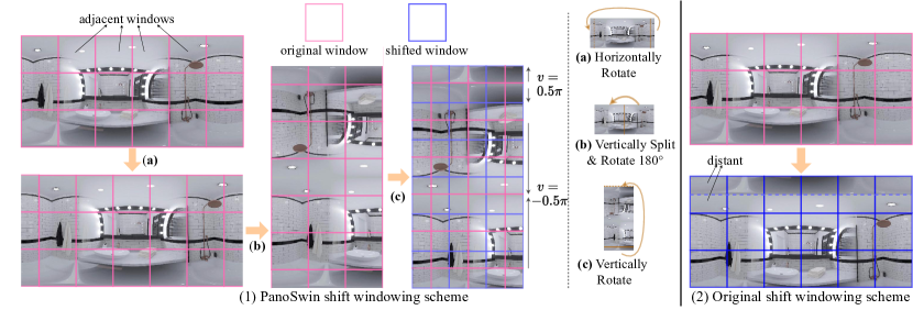
Figure 2: Pano-style/original shift windowing scheme comparison. The arrowed line in orange shows each conversion step.

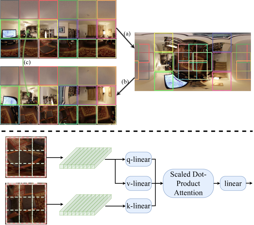
Figure 3: Top: our way to obtain a rotated window and perform pitch attention: (a) The pitch of the panorama is rotated by 90^∘; (b) we sample a rotated window in the rotated panorama for each original window; (c) window-wise attention is performed between old and rotated windows. The squares, distinguished by color, show each window conversion step. Bottom: detailed step (c).

3 Method

A panorama in equirectangular form is like the planar world map in our daily life. Each pixel of the panorama can be located by a longitude $u$ and a latitude $v$: $(u,v),u\in[-\pi,\pi),v\in[-0.5\pi,0.5\pi]$. Compared with Swin Transformer [21], the main novelty of PanoSwin lies in three aspects: pano-style shift windowing scheme, pitch attention module, and KP-based two-stage learning procedure.

3.1 Preliminaries of Swin Transformer

ViT[8] divides an image into patches and adopts a CNN to learn patch features. These patch features are then viewed as a sequence and fed into a transformer encoder. Although ViT[8] achieves good performances in various vision tasks, it suffers from high computation costs from global attention. Thus, Swin Transformer [21] proposed local multi-head self-attention (W-MSA), where image patches were further divided into small windows. Attention is only performed within each window. To enable information interaction among different windows, Swin Transformer[21] introduced Shifted Window-based Multi-head Self-Attention (SW-MSA), where the image is horizontally and vertically shifted to form a new one. As shown in Fig. 2-(2), W-MSA/SW-MSA is performed within each red/blue windows. However, shift windowing can bring distant pixels together. So attention masks are required in this process. Besides, Swin Transformer discards absolute positional embeddings [20] but adopts relative position bias[21, 12, 13], which specifies the relative coordinate difference between two patches within a window, instead of directly identifying the x/y coordinate[33].

3.2 Pano-style Shift Windowing Scheme

The problem of boundary discontinuity is brought by ERP. In a panorama, the left side ($u\approx-\pi$) and right side ($u\approx\pi$) are indeed connected. Also, all pixels around the north/south pole ($v\approx-0.5\pi/0.5\pi$) are adjacent. Traditional CNNs cannot deal with boundary discontinuity. The original shift windowing scheme in Swin Transformer[21] (Fig. 2-(2)) might capture wrong geometry continuity as well. Therefore, we propose a pano-style shift windowing scheme (PSW) and a pano-style shift windowing multi-head self-attention module (PSW-MSA), as shown in Fig. 2-(1). PSW can well capture the continuity around both side and polar boundaries of the panorama. There are three steps: (1) We horizontally shift the image, which enables the continuity around the left and right sides; (2) we split the image in half and rotate the right half by $\pi$ counterclockwise, which enables the continuities around north pole regions; (3) we vertically shift the image, which enables the continuities around south pole regions. Besides, pixels in each shifted window are connected, so no attention mask is required in our shift windowing scheme, further simplifying the attention process.

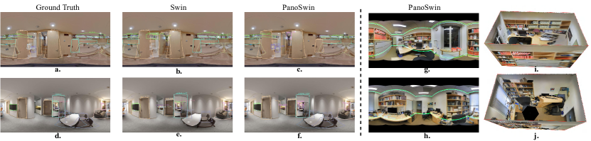
Figure 4: a-f.Detection visualization on 360-Indoor test set, where rectangular boxes are converted to spherical plane[3]. g-h.Layout prediction visualization on Stanford 2D-3D test set, green/lightblue curves shows the prediction/the groundtruth. i-j are layouts reconstructed from prediction of g-h.

3.3 Panoramic Rotation

Before going further, we need to introduce an operation that rotates the north pole of the panoramic image to a target coordinate. We define it as function $R$, as shown in Fig. 5. Let the north pole of the panorama be $P_{0}=(0,-0.5\pi)$. Given a target coordinate $P_{1}=(u_{1},v_{1})$ that $P_{0}$ will be rotated to, for a pixel $P=(u,v)$, we generate a new coordinate $P^{\prime}=(u^{\prime},v^{\prime})$ by $P^{\prime}=R(P,P_{1})$. By defining a Cartesian coordinate transition $\text{Sph}(P)=(x,y,z)$ for a given pixel $P=(u,v)$:

$$x=\sin(u)\cos(v),y=\cos(u)\cos(v),z=-\sin(v),$$ (1)

we can explain the function $R$ in a formula:

$$v^{\prime} = 2\text{asin}(\frac{1}{2}||\text{Sph}(P)-\text{Sph}(P_{1})||_{2})-0.5\pi,$$ (2)

$$P_{a}\hat{\otimes}P_{b} : \text{Sph}(P_{a})\otimes\text{Sph}(P_{b}),$$

$$u^{\prime} = \text{Angle}(P\hat{\otimes}P_{1},P_{0}\hat{\otimes}P_{1},(P_{0}\hat{\otimes}P_{1})\otimes P_{1}),$$

where $:$ stands for “define”; $\otimes$ is cross product. $\text{Angle}(\mathbf{x}_{1},\mathbf{x}_{2},\mathbf{x}_{3})$ gives the angle between vector $\mathbf{x}_{1}$ and vector $\mathbf{x}_{2}$, ranging from $-\pi$ to $\pi$; the counterclockwise direction is given by $\mathbf{x}_{3}$, that is, $\text{Angle}(\mathbf{x}_{3},\mathbf{x}_{2},\mathbf{x}_{3})<\pi$. It can be accomplished by arc cosine. To obtain a rotated panorama, we first calculate each target pixel coordinate by Eq. (2) and then sample a new panorama. Note that pitch rotations[28] and horizontal shifting[29] are special cases of $R$ when $u^{\prime}=0$ and $v^{\prime}=0$. Also, $R$ could be an approach to augment a panoramic image by setting $P_{1}$ randomly.

Computation analysis: If we only consider multiplication operation, the function $R$ consumes one $||\cdot||_{2}$, three Sph, and four $\otimes$. Since resultant $v^{\prime}$/$u^{\prime}$ should be scaled to image height/width, bilinear interpolation (BI-INT) is also required. Define a constant $K=\Omega(||\cdot||_{2})+3\Omega(\text{Sph})+4\Omega(\otimes)+\Omega(\text{BI-INT})=3\times 1+2\times 3+6\times 4+8=41$. Then, given a panorama of $H\times 2H$ size, we can give a lower bound for the computational complexity $\Omega(R)=2KH^{2}$.

3.4 Pitch Attention Module

Spatial distortion might severely hamper model performances, especially around polar regions. To target this problem, we propose a pitch attention module (PA). The workflow of the pitch attention module is shown in Fig. 2. Given a panorama $\mathcal{I}_{0}$ of size $H\times 2H$, in step (a), we rotate the pitch of $\mathcal{I}_{0}$ by $0.5\pi$ and obtain $\mathcal{I}_{1}$. That is, for each $P_{1}\in\mathcal{I}_{0}$, we obtain $P^{\prime}\in\mathcal{I}_{1}$ by $P^{\prime}=R((-\pi,0),P_{1})$. After the pitch rotation, the polar (resp. equator) regions of $\mathcal{I}_{0}$ are transformed to equator (resp. polar) regions of $\mathcal{I}_{1}$.

$\mathcal{I}_{0}$ is partitioned into windows like the W-MSA block in Swin transformer. Step (b) in Fig. 2 shows the way that we obtain the corresponding window in $\mathcal{I}_{1}$. For each window in $\mathcal{I}_{0}$, we locate the rotated window center in $\mathcal{I}_{1}$, and then sample a new square window in $\mathcal{I}_{1}$. At last, we perform cross attention [35, 37] between the old and new windows, where the old ones are the query and value, while the new ones are the key. The other details are the same as a W-MSA block of Swin transformer.

Computation analysis: Let the panorama of $H\times 2H\times C$ size be sliced into $h\times 2h$ patches and the window size be $M$, we can give the computational complexity lower bound: $\Omega(PA)=\Omega(R)+\underline{\Omega(\text{W-MSA})}+\Omega(\text{BI-INT})\times 2H^{2}=2(K+8)H^{2}+\underline{8h^{2}C^{2}+4M^{2}h^{2}C}$. Since we have $H=Mh$, $\Omega(PA)=\underline{8h^{2}C^{2}}+(\underline{4C}+2K+16)M^{2}h^{2}$, where $K=41$. When $C$ is large (e.g., $C=512$ as produced by many backbones), extra computational complexity introduced by pitch attention can be negligible.

In our network design, we insert a pitch attention module to the last of each backbone block, as shown in Tab. 3. Although pitch attention can enable interaction between adjacent windows, it does not replace PSW-MSA because (1) the interaction is not fair for all patches; (2) pitch attention brings more computation than PSW-MSA.

An alternative to our pitch attention module might be to adopt gnomonic projection[5] to generate tangent-plane windows, which are undistorted. However, (1) computation of gnomonic projection depends on viewpoints. It might be difficult to parallelize gnomonic projection for each window on GPU and therefore is more time-consuming; (2) we conduct experiments and find that tangent-plane windows yield no performance gain against pitch attention.

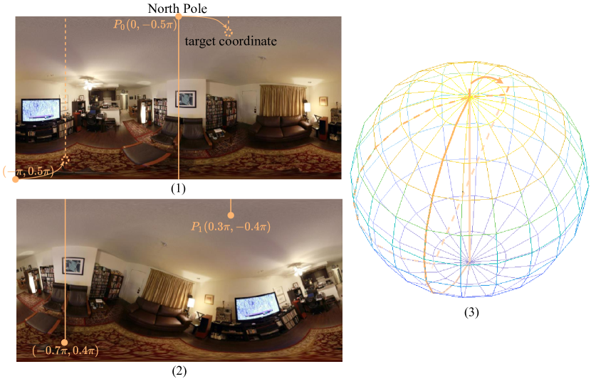
Figure 5: Illustration of panoramic rotation to target position $(0.3\pi,-0.4\pi)$: (1)/(2): the original/rotated panoramic image. (3): north pole rotation in sphere space. In formula, the figure shows $P^{\prime}=R(P,(0.3\pi,-0.4\pi))$.

Input: a downstream task loss $\mathcal{L}_{DS}$; a randomly initialied PanoSwin model $\mathcal{P}$.

Output: A trained PanoSwin model.

1 $\mathcal{A}^{plan}\leftarrow$ a set of planar augmentation methods, e.g., random resizing, cropping and rotation;

2 $\mathcal{A}^{pano}\leftarrow$ a set of pano-compatible augmentation methods, e.g., random panoramic rotation, flipping, color jittering;

3 Define $train(model,loss,augs)$ as a function that trains $model$ by optimizing $loss$ and enables augmentation approaches specified by $augs$;

4 $\mathcal{T}\leftarrow train(model=\mathcal{P}_{s},loss=\mathcal{L}_{DS},augs=\mathcal{A}^{plan}\cup\mathcal{A}^{pano})$;

5 $\mathcal{S}\leftarrow\mathcal{T};\quad fix(\mathcal{T});\quad fix(\alpha_{i,j}\;\text{of}\;S);\quad\mathcal{S}\leftarrow train(model=\mathcal{S}_{p},loss=\mathcal{L}_{DS}+\mathcal{L}_{KP},augs=\mathcal{A}^{pano})$;

return $\mathcal{S}$

Algorithm 1 two-stage learning paradigm.

3.5 Pano-style Positional Encodings

For relative positional biases, since the spherical distance between two patches in different windows varies largely by the window locations, we condition the relative positional biases on the great-circle distance:

$$d_{c}= \alpha_{i,j}\sin^{2}(\frac{v_{j}-v_{i}}{2})+$$ (3)

$$\alpha_{i,j}\cos(v_{j})\cos(v_{i})\sin^{2}(\frac{u_{j}-u_{i}}{2})+\beta_{i,j},$$

where $\alpha_{i,j}$ is great-circle bias and $\beta_{i,j}$ is planar bias, both learnable. They are looked up in a table, just like [21].

As for absolute positional embeddings, although Liu et. al.[21] show that relative positional biases are enough to reveal patch-wise geometric relations; therefore, absolute positional embeddings might not be necessary. However, panoramic geometric relations can be complicated. For example, on the same latitude, the left of a pixel can also be its right. Positional encodings based on Cartesian coordinates can strengthen pixel-level geometric information. We condition the absolute positional embeddings by both longitudes/latitudes and the sphere Cartesian coordinates. Several following fully connected layers encode $x,y,z,u,v$ into $d_{e}$-dimensional absolute positional embeddings, where $d_{e}$ is the patch embedding dimension. Then the positional embedding is added to the patch embedding.

3.6 Two-Stage Learning Paradigm

We devised a two-stage learning paradigm, as shown by Alg. 1. We call the first stage the planar stage and the second the panoramic stage. The planar stage learns planar knowledge, while the panoramic stage transfers common knowledge from planar images to panoramas.

The planar stage views the panorama as a planar image by various augmentation. Regular planar images can also be fed in this stage, but we try not to introduce additional training samples for a fair comparison. Let $\mathcal{L}_{DS}$ be the downstream task loss, e.g., a classification loss, or a bounding box regression loss. To enable PanoSwin to process planar images, we switch it to PanoSwin_s: (1) we let $\mathcal{I}_{1}\leftarrow\mathcal{I}_{0}$ in Sec. 3.4; (2) absolute positional embeddings are disabled; (3) great-circle bias $\alpha_{i,j}$ is set to 0 in Eq. (3). We let the obtained model be a teacher net $\mathcal{T}$.

In the panoramic stage, we initialize a student net $\mathcal{S}$ identical to $\mathcal{T}$. Then we $fix$ $\mathcal{T}$ and the planar bias $\beta_{i,j}$ of $\mathcal{S}$(Eq. (3)). Then we enable all previously disabled panoramic features of $\mathcal{S}$ and train $\mathcal{S}$ with panoramas. Since little distortion/discontinuity is introduced to central regions, we hope that $\mathcal{S}$ can mimic central signals of $\mathcal{T}$. For this purpose, we introduce a KP loss $\mathcal{L}_{KP}$ to preserve the pretrained knowledge in central regions simply using a weighted L2 loss. Given a panorama feature map $x$, we explain $\mathcal{L}_{KP}$ in formula:

$$\mathcal{L}_{KP}=\frac{1}{\sum^{N}_{i}w_{i}}\sum^{N}_{i}w_{i}||A(\mathcal{S}(x))^{(i)}-\mathcal{T}_{s}(x)^{(i)}||^{2}_{2},$$ (4)

where $w_{i}=\cos^{2}(v_{i})\cos^{2}(\frac{1}{2}u_{i})$ and $v_{i}$/$u_{i}$ is the latitude/longitude of pixel $i$; $A$ is an adaptation convolutional layer with a kernel size of $1\times 1$. The panoramic stage optimizes $\mathcal{L}_{DS}+w_{KP}\mathcal{L}_{KP}$ and only allows augmentation approaches compatible with panoramas, including panoramic augmentation like random panoramic rotation and non-geometric augmentation like random color jittering. $w_{KP}$ is a weight for $\mathcal{L}_{KP}$ that starts at 1 and then decays to 0. In the remaining paper, we will denote a PanoSwin obtained by the two-stage learning paradigm as PanoSwin⁺.

There could be many other knowledge distillation approaches to improve knowledge preservation performance for specific tasks[26, 39, 22], but $\mathcal{L}_{KP}$ shows a general way to transfer planar knowledge to panoramic tasks.

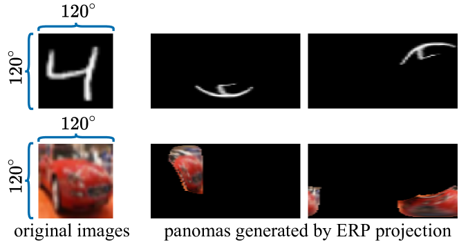
Figure 6: Cases of SPH-MNIST (top) and SPH-CIFAR10 (bottom)

No.	Backbone	error$\downarrow$	para.
M1	SpherePHD[16]	5.92	57k
M2	SphericalTrans.[2]	9.57	60k
M3	SphericalTrans-(Ext.)[2]	4.91	60k
M4	SGCN[38]	5.58	60k
M5	S2CNN[4]	6.97	58k
M6	SwinT13[21]	4.01	67k
M7	PanoSwinT12	3.08	66k
M8	GCNN[10]	17.21	282k
M10	SphereNet (BI)[5]	5.59	196k
M11	PanoSwinT8	2.25	191k
M12	VGG[25]+KTN[26]	2.06	294M
M13	SwinT[21]	1.53	28M
M14	PanoSwinT92	1.21	28M
M15	PanoSwinT	1.18	30M
M16	PanoSwinT+	1.15	30M

Table 1: SPH-MNIST classification result comparison.

No.	Backbone	acc$\uparrow$	para.
C1	SpherePHD[16]	59.20	57k
C2	SphericalTransformer[2]	58.21	60k
C3	SGCN[38]	60.72	60k
C4	S2CNN[4]	10.00	58k
C5	SwinT13[21]	60.46	67k
C6	PanoSwinT12	62.24	66k
C7	SwinT[21]	72.64	28M
C8	PanoSwinT92	74.50	28M
C9	PanoSwinT	74.84	30M
C10	PanoSwinT+	75.01	30M

Table 2: SPH-CIFAR10 classification result.

4 Experiments

4.1 Experimental Settings

structure alias	embedding dim	structure	para.
PanoSwinT8	8	[W, PSW, PA], PM, [W, PSW, PA], PM, [W, PSW, PA], PM, [W, PSW]	191k
PanoSwinT12	12	[W, PSW, PA], PM, [W, PSW]	66k
SwinT13[21]	13	[W, PSW, W], PM, [W, PSW]	67k
PanoSwinT92	92	[W,PSW,PA],PM,[W,PSW,PA],PM,[(W,PSW)*2,W,PA],PM,[W,PSW]	28M
SwinT[21]	96	[W,SW],PM,[W,SW],PM,[(W,SW)*3],PM,[W,SW]	28M
PanoSwinT	96	[W,PSW,PA],PM,[W,PSW,PA],PM,[(W,PSW)*2,W,PA],PM,[W,PSW]	30M

Table 3: PanoSwin architecture variants. W/SW: regular/shift windowing attention[21]. PSW: pano-style shift windowing attention. PA: pitch attention module. PM: patch merging[21]. ()*n denotes repeating n times. Refer to Supplementary for more details.

We conduct experiments on three tasks: panoramic classification, panoramic object detection, and panoramic layout estimation. Considering existing works on panorama representation learning vary a lot in model size, we design different PanoSwin backbones for a fair comparison in terms of model parameters, as shown in Tab. 3. To better remove spatial distortion, three convolutional layers are adopted to capture a larger reception field so as to learn better patch embedding.

For panoramic classification, we conduct experiments on SPH-MNIST and SPH-CIFAR10 datasets. SPH-MNIST and SPH-CIFAR10 are synthetic panoramic image datasets, as shown in Fig. 6, where the images of MNIST and CIFAR are projected with $120^{\circ}$ of horizontal and vertical FOV. The resultant panoramas are resized to $48\times 96$. We set learning rate $lr=0.001$ for light-weighted SwinT13, PanoSwinT8, and PanoSwinT12. For SwinT13, PanoSwinT12 and PanoSwinT, we set $lr=0.0001$. We adopt adam optimizer and batch size $b=48$ and train the model for 100/500 epochs in the planar/panoramic stage.

For panoramic object detection, we conduct experiments on the WHU street-view panoramic dataset[40] (StreetView in short) and 360-Indoor[3]. The object detection performance is evaluated by mean average precision with IOU=0.5 (mAP@0.5). (1) StreetView contains 600 street-view images, in which there are 5058 objects from four object categories. The training/test set split strictly follows [40], where one-third of images are used for training and the rest for testing. (2) 360-Indoor contains 3335 indoor images from 37 image categories, in which there are 89148 objects from 37 object categories. The training/test set split strictly follows [3]; 70% images are used for training and the rest for testing. Following [3], we train our model using conventional bounding boxes, that is, $xywh$ format. We adopt FasterRCNN+FPN[23, 18] as detector. One different setting is that, since PanoSwin can overcome side discontinuity, we allow the bounding box to cross the image side boundary by padding the pixels from the other side when training PanoSwin. We set so for Swin as well for a fair comparison. We set learning rate $lr=0.0002$, batch size $b=4$. We develop the detection framework based on the MMDetection toolbox[1]. The model is trained for 50/100 epochs in the planar/panoramic stage.

For panoramic room layout estimation, following HorizonNet[28], we train the model on the LayoutNet dataset[43], which is composed of PanoContext and the extended Stanford 2D-3D, consisting of 500 and 571 annotated panoramas respectively. Following HorizonNet[28], we train our model on the LayoutNet training set and test it on Stanford 2D-3D test set. We ONLY enable the panoramic stage in this task.

No.	Backbone	mAP@0.5$\uparrow$	para.
I1	R50[11] + COCO	33.1	72M
I2	SwinT[21] + COCO	33.8	45M
I3	PanoSwinT92 + COCO	35.6	45M
I4	R50[11]	20.6	72M
I5	R50[11] + SC[5]	21.1	72M
I6	SwinT[21]	24.0	45M
I7	PanoSwinT92	28.0	45M
I8	PanoSwinT	28.6	47M
I9	PanoSwinT+	29.4	47M

Table 4: Object detection performance comparison on 360-Indoor. R50 stands for ResNet50[11]. SC stands for SphereConv[5]. COCO denotes a pretraining procedure on MSCOCO[19].

No.	Backbone	mAP@0.5 $\uparrow$	para.
S1	VGG[25]+SCNN[41]	64.1	$>77$M
S2	R50[11]	68.2	72M
S3	R50[11]+SC[5]	69.4	72M
S4	SwinT	72.8	45M
S5	PanoSwinT92	75.4	45M
S5	PanoSwinT+	75.7	47M

Table 5: StreetView object detection performance comparison

No.	Backbone	3DIoU$\uparrow$	CE$\downarrow$	PE$\downarrow$	para.
P1	R50[11]	78.12	0.90	2.91	82M
P2	R50[11] + SC[5]	77.64	0.90	2.94	82M
P3	R34[11]	77.86	0.92	3.01	33M
P4	SwinT[21]	78.00	0.94	3.05	44M
P5	PanoSwinT92	78.10	0.92	2.99	44M
P6	R50[11]+ IN	84.66	0.66	2.04	82M
P7	R34[11] + IN	83.88	0.68	2.14	33M
P8	SwinT[21] + IN	84.04	0.66	2.07	44M
P9	PanoSwinT92 + IN	84.11	0.65	2.00	44M
P10	PanoSwinT + IN	84.21	0.65	1.98	46M

Table 6: Layout estimation comparison on Stanford-2D3D test set. “+ IN” denotes ImageNet[15] pretraining. CE/PE stands for corner error/pixel error.

4.2 Main Results

For panoramic classification, the results on SPH-MNIST/SPH-CIFAR10 are reported in Tab. 1/Tab. 2. Two important observations are: (1) Swin transformer can achieve results comparable to SOTA works with a similar number of model parameters, e.g., M6 v.s. M4, revealing that Swin is more generalizable than CNNs; (2) PanoSwin always beats Swin, e.g., M7 v.s. M6, M14 v.s. M13, indicating that PanoSwin can better learn panorama features.

Furthermore, on SPH-MNIST, we also test the trained SwinT13/PanoSwinT12 model on mnist test sets projected on the equator and polar regions. For SwinT13(M6), the test error rises from 2.94 to 5.41. For PanoSwinT12(M7), the test error rises from 2.87 to 3.32. The results further show that PanoSwin is more robust in handling spatial distortion.

For panoramic object detection, 360-Indoor and StreetView[40] are two real-world datasets, making the results more convincing. The results on these two datasets are reported in Tab. 4 and Tab. 5, respectively. The performance gain of PanoSwinT⁺ against SwinT is even larger, e.g. 5.4 on 360-Indoor. In addition, we investigate the detection performance of low-latitude regions against high-latitude regions. Viewpoints of low-latitude regions range from $-30^{\circ}$ to $30^{\circ}$, while viewpoints of the high-latitude region range from $\pm 60^{\circ}$ to $\pm 90^{\circ}$). We find out that mAP@50 drops by 1.9/3.5/2.0/5.8 using PanoSwinT92/SwinT/ResNet50+SC/ResNet50. It reveals that (1) attention mechanisms are better than CNN at handling spatial distortion; (2) our proposed PanoSwin is the most robust to deal with polar spatial distortion.

Results on panoramic layout estimation are reported in Tab. 6. Fig. 4 visualizes the layouts estimated by PanoSwin. PanoSwinT92 outperforms other backbones but ResNet50. Although HorizonNet+PanoSwinT92 has almost only half parameters as HorizonNet+ResNet50 does, PanoSwinT92 still outperforms ResNet50 in corner error and pixel error with ImageNet[15] pretraining, and is only slightly exceeded by ResNet50 without pretraining. The results contradict the larger advantage of PanoSwin in object detection. We conjecture that this is because (1) layout estimation needs pixel-level understanding more than object-level understanding. So spatial distortion is no longer a big problem; (2) layout estimation depends on wall corners instead of polar regions. So polar boundary discontinuity is not important; (3) HorizonNet designs a Bi-LSTM to overcome side boundary discontinuity. Therefore, PanoSwin shows little advantage in layout estimation performance.

Tab. 7 reports inference speed. It shows that (1) pitch attention brings non-negligible computation (PST v.s. PST_s); (2) PanoSwin is efficient when compared against other panoramic backbones (PST v.s. KTN/SphereNet), which is because PanoSwin introduces few non-parallelizable operations. On the contrary, many existing works introduce operations that cannot be parallelized. For example, KTN[26] adopts different convolutions of various kernel sizes in different latitudes, resulting in a time-consuming “for” loop in forwarding. While SphereNet[5] also takes a long time to calculate uniform sampling coordinates for each convolution.

	PST	PSTs	SwinT	KTN[26]	PST8	SN
para.	30M	30M	28M	294M	191k	196k
CPU$\downarrow$	1.207	1.018	0.982	5.136	0.186	0.682
GPU$\downarrow$	0.042	0.015	0.010	3.842	0.021	0.025

Table 7: Single image(512x1024 size) inference speed comparison (second). PST/SN is short for PanoSwinT/SphereNet[5].

No.	alternative	SM$\downarrow$	3I$\uparrow$
A1	only planar stage	1.76	26.8
A2	only panoramic stage	1.18	25.9
A3	PSW $\rightarrow$ W	1.43	28.0
A4	PA $\rightarrow$ W	2.01	27.9
A5	swin rel. pos.[21]	1.31	28.3
A6	remove abs. pos.	1.19	29.0
A7	$w_{i}\leftarrow 1$ in $\mathcal{L}_{KP}$	1.26	27.6
A8	$w/o$ $\mathcal{L}_{KP}$	1.18	28.6
A9	full model+	1.15	29.4

Table 8: Ablation of SPH-MNIST classification and 360-Indoor object detection using PanoSwinT. Column “SM”/“3I” reports test error on SPH-MNIST/mAP@50 on 360-Indoor. “swin rel. pos.” denotes replacing our proposed pano-style relative position biases with the original swin-style relative biases[21].

4.3 Ablation Study

We conduct ablation experiments on SPH-MNIST classification and 360-Indoor object detection. The results are reported in Tab. 8. On the one hand, a general difference revealed in the results between these two datasets is that the 360-Indoor dataset is more sensitive to our proposed modules than SPH-MNIST, e.g., setting A2, A6, and A8. We consider that this is because SPH-MNIST is larger but simpler than 360-Indoor. Therefore some modules like planar-stage training, pano-style absolute positional embeddings, and $\mathcal{L}_{KP}$ only result in a marginal performance gain.

On the other hand, we have observations for different modules: (1) A1 and A2 show that both the planar stage and panoramic stage are necessary, implying that planar knowledge is also helpful for panorama representation learning. Indeed, various planar augmentation approaches can be very effective in improving model performance. But some of the existing works[5, 2] might not emphasize the importance of planar knowledge.  (2) A3 and A4 validate effectiveness of PSW and PA. Fig. 4.d-f also reveals so. Detection on the table and the chair on the left/right side shows that PSW effectively bridges side discontinuity. Detection on the large white table in the middle bottom implies that PA can solve spatial distortion.  (3) A5 and A6 demonstrate the effectiveness of absolute position encodings and relative position biases.  (4) A8 shows that central knowledge preservation accomplished by $\mathcal{L}_{KP}$ can well improve model performance. While A7 shows that naive $\mathcal{L}_{KP}^{\prime}$ even results in a performance drop, implying that polar and side planar knowledge from the teacher net $\mathcal{T}$ is not reliable.

5 Conclusion

Spatial distortion and boundary discontinuity are two fundamental problems in panorama understanding. In this paper, we propose PanoSwin to learn panorama features in the ERP form, which is simple and fast. In PanoSwin, we first propose a pano-style shift windowing scheme that bridges discontinued boundaries. Then a novel pitch attention module is proposed to overcome spatial distortion. Moreover, to transfer common knowledge from planar images to panoramic tasks, we contribute a KP-based two-stage learning paradigm. Experiments demonstrate that, without introducing many extra parameters and computation over Swin[21], PanoSwin achieves SOTA results in various tasks, including panoramic classification, panoramic object detection, and panoramic layout estimation. In the future, we will further extend PanoSwin to more tasks like panoramic segmentation and panoramic depth estimation.

Acknowledgement This work was supported by the National Key Research and Development Program of China, No.2018YFB1402600.

References

- [1] Kai Chen, Jiaqi Wang, Jiangmiao Pang, Yuhang Cao, Yu Xiong, Xiaoxiao Li, Shuyang Sun, Wansen Feng, Ziwei Liu, Jiarui Xu, Zheng Zhang, Dazhi Cheng, Chenchen Zhu, Tianheng Cheng, Qijie Zhao, Buyu Li, Xin Lu, Rui Zhu, Yue Wu, Jifeng Dai, Jingdong Wang, Jianping Shi, Wanli Ouyang, Chen Change Loy, and Dahua Lin. Mmdetection: Open mmlab detection toolbox and benchmark. arXiv preprint arXiv:1906.07155, 2019.
- [2] Sungmin Cho, Raehyuk Jung, and Junseok Kwon. Spherical transformer. CoRR, abs/2202.04942, 2022.
- [3] Shih-Han Chou, Cheng Sun, Wen-Yen Chang, Wan Ting Hsu, Min Sun, and Jianlong Fu. 360-indoor: Towards learning real-world objects in 360° indoor equirectangular images. In Winter Conference on Applications of Computer Vision (WACV), 2020.
- [4] Taco S. Cohen, Mario Geiger, Jonas Köhler, and Max Welling. Spherical cnns. In International Conference on Learning Representations (ICLR), 2018.
- [5] Benjamin Coors, Alexandru Paul Condurache, and Andreas Geiger. Spherenet: Learning spherical representations for detection and classification in omnidirectional images. In European Conference on Computer Vision (ECCV), 2018.
- [6] Michaël Defferrard, Martino Milani, Frédérick Gusset, and Nathanaël Perraudin. Deepsphere: a graph-based spherical CNN. In International Conference on Learning Representations (ICLR), 2020.
- [7] Jacob Devlin, Ming-Wei Chang, Kenton Lee, and Kristina Toutanova. BERT: pre-training of deep bidirectional transformers for language understanding. In Jill Burstein, Christy Doran, and Thamar Solorio, editors, the North American Chapter of the Association for Computational Linguistics: Human Language Technologies (NAACL-HLT), 2019.
- [8] Alexey Dosovitskiy, Lucas Beyer, Alexander Kolesnikov, Dirk Weissenborn, Xiaohua Zhai, Thomas Unterthiner, Mostafa Dehghani, Matthias Minderer, Georg Heigold, Sylvain Gelly, Jakob Uszkoreit, and Neil Houlsby. An image is worth 16x16 words: Transformers for image recognition at scale. CoRR, abs/2010.11929, 2020.
- [9] Haoqi Fan, Bo Xiong, Karttikeya Mangalam, Yanghao Li, Zhicheng Yan, Jitendra Malik, and Christoph Feichtenhofer. Multiscale vision transformers. In Computer Vision and Pattern Recognition (CVPR), 2021.
- [10] Pascal Frossard and Renata Khasanova. Graph-based classification of omnidirectional images. In International Conference on Computer Vision Workshops (ICCV workshops), 2017.
- [11] Kaiming He, Xiangyu Zhang, Shaoqing Ren, and Jian Sun. Deep residual learning for image recognition. In Computer Vision and Pattern Recognition (CVPR), 2016.
- [12] Han Hu, Jiayuan Gu, Zheng Zhang, Jifeng Dai, and Yichen Wei. Relation networks for object detection. In Computer Vision and Pattern Recognition (CVPR), 2018.
- [13] Han Hu, Zheng Zhang, Zhenda Xie, and Stephen Lin. Local relation networks for image recognition. In Computer Vision and Pattern Recognition (CVPR), 2019.
- [14] Gao Huang, Zhuang Liu, Laurens van der Maaten, and Kilian Q. Weinberger. Densely connected convolutional networks. In Computer Vision and Pattern Recognition (CVPR), 2017.
- [15] Alex Krizhevsky, Ilya Sutskever, and Geoffrey E Hinton. Imagenet classification with deep convolutional neural networks. Communications of the ACM, 2017.
- [16] Yeon Kun Lee, Jaeseok Jeong, Jong Seob Yun, Wonjune Cho, and Kuk-Jin Yoon. Spherephd: Applying cnns on a spherical polyhedron representation of 360deg images. In Computer Vision and Pattern Recognition (CVPR), 2019.
- [17] Bei Li, Yi Jing, Xu Tan, Zhen Xing, Tong Xiao, and Jingbo Zhu. Transformer: Slow-fast transformer for machine translation. arXiv preprint arXiv:2305.16982, 2023.
- [18] Tsung-Yi Lin, Piotr Dollár, Ross Girshick, Kaiming He, Bharath Hariharan, and Serge Belongie. Feature pyramid networks for object detection. In Computer Vision and Pattern Recognition (CVPR), 2017.
- [19] Tsung-Yi Lin, Michael Maire, Serge Belongie, James Hays, Pietro Perona, Deva Ramanan, Piotr Dollár, and C Lawrence Zitnick. Microsoft coco: Common objects in context. In European Conference on Computer Vision (ECCV), 2014.
- [20] Zhixin Ling, Zhen Xing, Jiangtong Li, and Li Niu. Multi-level region matching for fine-grained sketch-based image retrieval. In Proceedings of the 30th ACM International Conference on Multimedia, pages 462–470, 2022.
- [21] Ze Liu, Yutong Lin, Yue Cao, Han Hu, Yixuan Wei, Zheng Zhang, Stephen Lin, and Baining Guo. Swin transformer: Hierarchical vision transformer using shifted windows. In International Conference on Computer Vision (ICCV), 2021.
- [22] Zhidan Liu, Zhen Xing, Xiangdong Zhou, Yijiang Chen, and Guichun Zhou. 3d-augmented contrastive knowledge distillation for image-based object pose estimation. In Proceedings of the 2022 International Conference on Multimedia Retrieval, 2022.
- [23] Shaoqing Ren, Kaiming He, Ross B. Girshick, and Jian Sun. Faster R-CNN: Towards real-time object detection with region proposal networks. IEEE Transactions on Pattern Analysis and Machine Intelligence (T-PAMI), 2017.
- [24] Zhijie Shen, Chunyu Lin, Kang Liao, Lang Nie, Zishuo Zheng, and Yao Zhao. Panoformer: Panorama transformer for indoor 360° depth estimation. CoRR, abs/2203.09283, 2022.
- [25] Karen Simonyan and Andrew Zisserman. Very deep convolutional networks for large-scale image recognition. arXiv preprint arXiv:1409.1556, 2014.
- [26] Yu-Chuan Su and Kristen Grauman. Kernel transformer networks for compact spherical convolution. In Computer Vision and Pattern Recognition (CVPR), 2019.
- [27] Yu-Chuan Su and Kristen Grauman. Learning spherical convolution for fast features from 360 imagery. Advances in Neural Information Processing Systems (NIPS), 2017.
- [28] Cheng Sun, Chi-Wei Hsiao, Min Sun, and Hwann-Tzong Chen. Horizonnet: Learning room layout with 1d representation and pano stretch data augmentation. In Computer Vision and Pattern Recognition (CVPR), 2019.
- [29] Cheng Sun, Min Sun, and Hwann-Tzong Chen. Hohonet: 360 indoor holistic understanding with latent horizontal features. In Computer Vision and Pattern Recognition (CVPR), 2021.
- [30] Christian Szegedy, Sergey Ioffe, Vincent Vanhoucke, and Alexander A. Alemi. Inception-v4, inception-resnet and the impact of residual connections on learning. In AAAI Conference on Artificial Intelligence (AAAI), 2017.
- [31] Hugo Touvron, Matthieu Cord, Matthijs Douze, Francisco Massa, Alexandre Sablayrolles, and Hervé Jégou. Training data-efficient image transformers & distillation through attention. In International Conference on Machine Learning (ICML), 2021.
- [32] Hugo Touvron, Matthieu Cord, and Hervé Jégou. Deit iii: Revenge of the vit. arXiv preprint arXiv:2204.07118, 2022.
- [33] Ashish Vaswani, Noam Shazeer, Niki Parmar, Jakob Uszkoreit, Llion Jones, Aidan N. Gomez, Lukasz Kaiser, and Illia Polosukhin. Attention is all you need. In Advances in Neural Information Processing Systems (NIPS), 2017.
- [34] Haiping Wu, Bin Xiao, Noel Codella, Mengchen Liu, Xiyang Dai, Lu Yuan, and Lei Zhang. Cvt: Introducing convolutions to vision transformers. In International Conference on Computer Vision (ICCV), 2021.
- [35] Zhen Xing, Yijiang Chen, Zhixin Ling, Xiangdong Zhou, and Yu Xiang. Few-shot single-view 3d reconstruction with memory prior contrastive network. In ECCV, 2022.
- [36] Zhen Xing, Qi Dai, Han Hu, Jingjing Chen, Zuxuan Wu, and Yu-Gang Jiang. Svformer: Semi-supervised video transformer for action recognition. In Computer Vision and Pattern Recognition (CVPR), 2023.
- [37] Zhen Xing, Hengduo Li, Zuxuan Wu, and Yu-Gang Jiang. Semi-supervised single-view 3d reconstruction via prototype shape priors. In ECCV, 2022.
- [38] Qin Yang, Chenglin Li, Wenrui Dai, Junni Zou, Guo-Jun Qi, and Hongkai Xiong. Rotation equivariant graph convolutional network for spherical image classification. In Computer Vision and Pattern Recognition (CVPR), 2020.
- [39] Zhendong Yang, Zhe Li, Xiaohu Jiang, Yuan Gong, Zehuan Yuan, Danpei Zhao, and Chun Yuan. Focal and global knowledge distillation for detectors. In Computer Vision and Pattern Recognition (CVPR), 2022.
- [40] Dawen Yu and Shunping Ji. Grid based spherical cnn for object detection from panoramic images. Sensors, 2019.
- [41] Dawen Yu and Shunping Ji. Grid based spherical CNN for object detection from panoramic images. Sensors, 2019.
- [42] Kun Yuan, Shaopeng Guo, Ziwei Liu, Aojun Zhou, Fengwei Yu, and Wei Wu. Incorporating convolution designs into visual transformers. In International Conference on Computer Vision (ICCV), 2021.
- [43] Chuhang Zou, Alex Colburn, Qi Shan, and Derek Hoiem. Layoutnet: Reconstructing the 3d room layout from a single rgb image. In Computer Vision and Pattern Recognition (CVPR), 2018.