Exploring the NANOGrav Signal and Planet-mass Primordial Black Holes through Higgs Inflation

Abstract

The data recently released by the North American Nanohertz Observatory for Gravitational Waves provides compelling evidence supporting the existence of a stochastic signal that aligns with a gravitational-wave background. We show this signal can be the scalar-induced gravitational waves from the Higgs inflation model with the parametric amplification mechanism. Such a gravitational-wave background naturally predicts the substantial existence of planet-mass primordial black holes, which can be planet 9 in our solar system and the lensing objects for the ultrashort-timescale microlensing events observed by the Optical Gravitational Lensing Experiment. The future observations of stochastic gravitational wave background by pulsar timing arrays and planet-mass primordial black holes provide such a possibility to give further confirmations on Higgs inflation, which unifies two fundamental aspects of theoretical physics, particle physics and cosmology.

Introduction. Subsequent to the discernment of gravitational waves (GWs) arising from the coalescence of black holes and neutron stars by LIGO-Virgo Abbott et al. (2016a, b, 2017a, 2017b, 2017c, 2017d), the forthcoming inspiring discovery may be the identification of the stochastic gravitational-wave background (SGWB), which has a large frequency range from $10^{-20}$ Hz to $10^{8}$ Hz. The pulsar timing array (PTA) possesses the capability to ascertain the lower-frequency band of the SGWB reaching as far as around $10^{-8}$ Hz, which proves to be a valuable window for detecting GWs originating from the early stages of the Universe. Recently, the North American Nanohertz Observatory for Gravitational Waves (NANOGrav) Agazie et al. (2023a, b), as well as Parkers Pulsar Timing Array (PPTA) Zic et al. (2023); Reardon et al. (2023), European Pulsar Timing Array (EPTA) Antoniadis et al. (2023a, b), and Chinese Pulsar Timing Array (CPTA) Xu et al. (2023) have reported compelling evidence for a common-spectrum signal consistent with the Hellings-Downs spatial correlations Hellings and Downs (1983), supporting the existence of a stochastic signal that aligns with a SGWB. While a lot of potential sources exist within the PTA window Li et al. (2019); Vagnozzi (2021); Chen et al. (2021); Wu et al. (2022a); Chen et al. (2022a); Benetti et al. (2022); Chen et al. (2022b); Ashoorioon et al. (2022); Wu et al. (2022b, 2023a); Falxa et al. (2023); Wu et al. (2023b); Dandoy et al. (2023); Madge et al. (2023), the discernment of whether this signal originates from astrophysical or cosmological phenomena remains the subject of rigorous and comprehensive investigation Afzal et al. (2023); Antoniadis et al. (2023c); King et al. (2023a); Niu and Rahat (2023); Bi et al. (2023); Liu et al. (2023a); Vagnozzi (2023); Han et al. (2023); Li et al. (2023); Franciolini et al. (2023a); Shen et al. (2023); Kitajima et al. (2023); Franciolini et al. (2023b); Addazi et al. (2023); Cai et al. (2023); Inomata et al. (2023); Wang et al. (2023); Murai and Yin (2023); Li and Xie (2023); Anchordoqui et al. (2023); Liu et al. (2023b); Zhu et al. (2023); Abe and Tada (2023); Ghosh et al. (2023); Figueroa et al. (2023); Yi et al. (2023a); Wu et al. (2023c); Li (2023); Geller et al. (2023); You et al. (2023); Antusch et al. (2023); Ye and Silvestri (2023); Hosseini Mansoori et al. (2023); Jin et al. (2023); Zhang et al. (2023); Valbusa Dall’Armi et al. (2023); De Luca et al. (2023); Gorji et al. (2023); Das et al. (2023); Yi et al. (2023b); Ellis et al. (2023); He et al. (2023); Zhao et al. (2023); Balaji et al. (2023); Kawasaki and Murai (2023); Cannizzaro et al. (2023); King et al. (2023b); Maji and Park (2023); Bhaumik et al. (2023).

One potential explanation for the observed signal is the scalar-induced gravitational waves (SIGWs) generated by the primordial curvature perturbations at small scales, which is favored by the NANOGrav data over the supermassive black hole binaries (SMBHBs) scenario through Bayesian analysis Afzal et al. (2023). When the primordial curvature perturbations attain considerable magnitudes, they can produce a significant SGWB via second-order effects arising from the nonlinear coupling of perturbations. Moreover, the emergence of PBHs can be triggered by the presence of large curvature perturbations Zel’dovich and Novikov (1967); Hawking (1971); Carr and Hawking (1974). In recent years, PBHs have attracted considerable interest Belotsky et al. (2014); Carr et al. (2016); Garcia-Bellido and Ruiz Morales (2017); Carr et al. (2017); Germani and Prokopec (2017); Chen et al. (2019); Liu et al. (2019a); Chen and Huang (2018); Cai et al. (2019); Liu et al. (2019b); Fu et al. (2019); Liu et al. (2020a); Cai et al. (2020); Chen and Huang (2020); Liu et al. (2020b); Fu et al. (2020); De Luca et al. (2021a); Vaskonen and Veermäe (2021); De Luca et al. (2021b); Domènech and Pi (2022); Hütsi et al. (2021); Chen et al. (2022c); Kawai and Kim (2021); Braglia et al. (2021); Liu et al. (2023c); Braglia et al. (2023); Zheng et al. (2023); Liu et al. (2023d); Chen et al. (2023); Guo et al. (2023) (see reviews Sasaki et al. (2018); Carr et al. (2021); Carr and Kuhnel (2020)) due to their potential as a promising candidate for dark matter Sasaki et al. (2018); Carr et al. (2021); Carr and Kuhnel (2020). Furthermore, they offer a plausible explanation for the observed phenomena of binary black holes detected by LIGO-Virgo-KAGRA Bird et al. (2016); Sasaki et al. (2016).

To generate significant SIGWs compatible with the recent PTA signal, the amplitude of the primordial curvature power spectrum in the small scales needs to be enhanced by around seven orders of magnitude compared with that in the cosmic microwave background (CMB) scale. The parametric amplification mechanism proposed in Ref. Cai et al. (2020) can amplify the primordial curvature power spectrum independent of the inflation potential. In this letter, we show that the recently reported NANOGrav signal can be the SIGWs from the Higgs inflation model with the parametric amplification mechanism. Such an SGWB naturally predicts the substantial existence of planet-mass PBHs, which can be planet 9 in our solar system Scholtz and Unwin (2020) and the lensing objects for the ultrashort-timescale microlensing events observed by the Optical Gravitational Lensing Experiment (OGLE) Mróz et al. (2017); Niikura et al. (2019a).

Parametric amplification and Higgs inflation. The primordial curvature perturbations $\mathcal{R}$ of the canonical inflation model in the Fourier space satisfy the Mukhanov-Sasaki equation

$$u^{\prime\prime}_{k}+(k^{2}-z^{\prime\prime}/z)u_{k}=0,$$ (1)

where $u=-z\mathcal{R}$, $z=a\dot{\phi}/H$, and

$$\frac{z^{\prime\prime}}{z}=2a^{2}H^{2}\left(1+\frac{3}{2}\delta+\epsilon+\frac{1}{2}\delta^{2}+\frac{1}{2}\epsilon\delta+\frac{1}{2H}\dot{\epsilon}+\frac{1}{2H}\dot{\delta}\right),$$ (2)

with the slow-roll parameters $\epsilon\equiv-\dot{H}/H^{2}$ and $\delta\equiv\ddot{\phi}/H\dot{\phi}$ Kodama and Sasaki (1984); Mukhanov et al. (1992). To obtain the parametric amplification mechanism, we assume that the potential consists of a small periodic structure $\delta V$, with $\delta V\ll\bar{V}$, added to a single-field slow-roll inflationary potential $\bar{V}$ Cai et al. (2020). Specifically, it can be expressed as

$$V(\phi)=\bar{V}(\phi)+\delta V(\phi)$$ (3)

where the oscillatory part is

$$\delta V(\phi)=\xi\cos(\phi/\phi_{*})\Theta(\phi;\phi_{s},\phi_{e}).$$ (4)

Here, $\xi,\phi_{*},\phi_{s}$, and $\phi_{e}$ represent the magnitude, period, starting and ending points of the structure, respectively, and $\Theta(\phi;\phi_{s},\phi_{e})\equiv\Theta(\phi_{e}-\phi)\Theta(\phi-\phi_{s})$ is constructed by the Heaviside step function $\Theta$. We suppose that the small periodic structure has a negligible impact on the background evolution. During oscillatory phase, i.e., the time interval from $\phi_{s}$ to $\phi_{e}$, $\dot{\phi}$ and $\bar{V}_{,\phi}$ can be ignored, while $\ddot{\phi}$ and $\delta V_{,\phi}$ should be emphasized. Using the background equation, we obtain the approximations $\phi\approx\phi_{s}+\dot{\phi}_{s}(t-t_{s})$ and $\ddot{\phi}\approx\xi\sin(\phi/\phi_{*})/\phi_{*}$. Therefore, during the oscillatory phase, we have $\frac{z^{\prime\prime}}{z}\approx a^{2}H\dot{\delta}\approx a^{2}\frac{\xi}{\phi_{*}^{2}}\cos(\frac{\phi}{\phi_{*}})$, if $H\ll 1$. This leads to the equation of motion for the perturbations $u_{k}$

$$\ddot{u}_{k}+H\dot{u}_{k}+\left[\frac{k^{2}}{a^{2}}-\frac{\xi}{\phi_{*}^{2}}\cos(\frac{\phi}{\phi_{*}})\right]u_{k}=0.$$ (5)

When focusing on the small scales ($k\gg aH$), the term $H\dot{u}_{k}$ loses significance and becomes negligible. Consequently, we are able to represent equation (5) in the following form,

$$\frac{d^{2}u_{k}}{dx^{2}}+\left[A_{k}(x)-2q\cos 2x\right]u_{k}=0,$$ (6)

where $x=t\dot{\phi}_{s}/(2\phi_{*})+(\phi_{s}-\dot{\phi}_{s}t_{s})/(2\phi_{*})$, $A_{k}(x)=k^{2}/(k_{*}^{2}a^{2})$, $k_{*}=|\dot{\phi}_{s}|/(2\phi_{*})$, $q=2\xi/\dot{\phi}_{s}^{2}$. The analytical results of the power spectrum is

$$\mathcal{P}_{\mathcal{\mathcal{R}}}(k)\approx A_{s}\left(\frac{k}{k_{p}}\right)^{n_{s}-1}\mathcal{A}^{2}(k).$$ (7)

Here, $A_{s}$ and $n_{s}$ represent the amplitude and scalar spectral index of the power spectrum at the pivot scale $k_{p}=0.05~{}\mathrm{Mpc}^{-1}$. The amplification factor $\mathcal{A}(k)$ is explicitly defined as

$$\mathcal{A}(k)\equiv|u_{k}(t_{e})|/|u_{k}(t_{s})|\approx\exp\left(\int_{t_{s}}^{t_{e}}\mu_{k}(t)k_{*}dt\right),$$ (8)

where

$$\mu_{k}(t)=\Re\left(\sqrt{\left(\frac{q}{2}\right)^{2}-\left(\frac{k}{k_{*}a(t)}-1\right)^{2}}\right).$$ (9)

and $\Re(y)$ denotes the real component of the quantity $y$.

For the Higgs inflation, the action is Bezrukov and Shaposhnikov (2008)

$$S=\int d^{4}x\sqrt{-g}\left[\frac{M_{\mathrm{pl}}^{2}}{2}R+\xi H_{\mathrm{SM}}^{\dagger}H_{\mathrm{SM}}R+\mathcal{L}_{\mathrm{SM}}\right],$$ (10)

where $\mathcal{L}_{\mathrm{SM}}$ is the Standard Model part, $H_{\mathrm{SM}}$ is the Higgs field, $\xi$ is a dimensionless coupling constant, and $M_{\mathrm{pl}}=1/\sqrt{8\pi G}$ is the reduced Planck mass. In the unitary gauge $H_{\mathrm{SM}}=(0,h/\sqrt{2})^{T}$, the action of the Higgs inflation in the Jordan frame becomes

$$S=\int d^{4}x\sqrt{-g}\left[\frac{M_{\mathrm{pl}}^{2}+\xi h^{2}}{2}R-\frac{1}{2}(\partial h)^{2}-V_{h}(h)\right].$$ (11)

By using the condition that the energy of the Higgs field $h$ during the inflation epoch is significantly greater than the vacuum expectation value $v_{\mathrm{EW}}\simeq 250\mathrm{GeV}$, the Higgs potential can be expressed in a simplified form as $V_{h}(h)=\lambda h^{4}/4$. In the following, we set the reduced Planck mass and the speed of light to unity, $M_{\mathrm{pl}}=c=1$.

For the homogeneous and isotropic Universe, the background equations are

$$H^{2}+\frac{2\xi h\dot{h}}{1+\xi h^{2}}H=\frac{1}{3\left(1+\xi h^{2}\right)}\left[\frac{1}{2}\dot{h}^{2}+V_{h}(h)\right],$$ (12)

$$A(h)(\ddot{h}+3H\dot{h})+B(h)\dot{h}^{2}+V_{h}^{\prime}(h)=\frac{4\xi\phi V_{h}(h)}{1+\xi h^{2}},$$ (13)

where $A(h)=1+\frac{6\xi^{2}h^{2}}{1+\xi h^{2}}$, $B(h)=\frac{(\xi+6\xi^{2})h}{1+\xi h^{2}}$, $H=\dot{a}/a$ is the Hubble parameter, $a$ is the cosmic scale factor, a ‘dot’ denotes the derivative with respect to the cosmic time $t$, and $V_{h}^{\prime}=dV_{h}/dh$. The equation for the primordial curvature perturbation $\mathcal{R}_{k}$ satisfies the Mukhanov-Sasaki equation (1) with Hwang (1997)

$$z=\frac{a\dot{h}}{H}\sqrt{\frac{\left(1+\xi h^{2}\right)\left(1+\xi h^{2}+6\xi^{2}h^{2}\right)}{\left(1+\xi h^{2}+\xi h\dot{h}/H\right)^{2}}}.$$ (14)

On the other hand, if the coupling constant $\xi$ is large enough, in the Einstein frame the Higgs inflation model becomes

$$S=\int d^{4}x\sqrt{-g}\left[\frac{1}{2}R-\frac{1}{2}(\partial\phi)^{2}-V_{E}(\phi)\right],$$ (15)

where $\phi$ is the inflation field in the Einstein frame, and it can be related to the the inflation field $h$ in the Jordan frame by Bezrukov and Shaposhnikov (2008)

$$h=\frac{1}{\sqrt{\xi}}\exp\left(\frac{\phi}{\sqrt{6}}\right).$$ (16)

The potential in the Einstein frame is Bezrukov and Shaposhnikov (2008)

$$V_{E}(\phi)\approx\frac{\lambda}{4\xi^{2}}\left[1+\exp\left(-\frac{2\phi}{\sqrt{6}}\right)\right]^{-2}.$$ (17)

To obtain the parametric amplification, the potential (17) needs an extra small oscillatory part as displayed in equations (3) and (4). Combining the approximate relation of the fields between the Jordan and Einstein frames (16) and the cosine form (4), we can obtain a similar oscillatory part potential in the Jordan frame, where the simplest form is

$$\delta V_{h}(h)=b\cos\left(\frac{1}{h_{*}}\ln h\right)\Theta(h;h_{s},h_{e}).$$ (18)

Therefore, if the Higgs potential has a small oscillatory part $V(h)=V_{h}(h)+\delta V_{h}(h)$, the Mukhanov-Sasaki equation can become the Mathieu equation during the oscillatory phase, and the parametric amplification mechanism can be applied. Consequently, the primordial curvature power spectrum from the Higgs inflation can be enhanced. Furthermore, the oscillatory part (18) only exists in the inflation region $h_{e}\leq h\leq h_{s}$, and disappears after the scale $h_{e}$, leading to the recovery of the usual Higgs inflation model.

SIGWs and PBHs. Within the context of the Newtonian gauge, the perturbed metric finds expression as follows:

$$ds^{2}=a^{2}(\tau)\left\{-(1+2\Phi)\mathrm{d}\tau^{2}+[(1-2\Phi)\delta_{ij}+h_{ij}]\mathrm{d}x^{i}\mathrm{d}x^{j}\right\},$$ (19)

Here, $\Phi$ denotes the Bardeen potential, and $h_{ij}$ signifies the tensor perturbations. It is pertinent to underscore that our focus excludes the influences stemming from first-order gravitational waves, vector perturbations, and anisotropic stress. Prior investigations (Baumann et al. (2007); Weinberg (2004); Watanabe and Komatsu (2006)) have duly substantiated the minor nature of their contributions. Following the Refs. Kohri and Terada (2018); Espinosa et al. (2018), the energy density of SIGWs at the epoch of matter-radiation equality can be presented as

$$\Omega_{\mathrm{GW}}(k)=\int_{0}^{\infty}\mathrm{d}v\int_{|1-v|}^{|1+v|}\mathrm{d}u\mathcal{T}(u,v){P}_{\zeta}(vk){P}_{\zeta}(uk),$$ (20)

where ${P}_{\zeta}$ is the primordial power spectrum of curvature perturbations and

$$\mathcal{T}(u,v)= \frac{3}{1024v^{8}u^{8}}\left[4v^{2}-\left(v^{2}-u^{2}+1\right)^{2}\right]^{2}\left(v^{2}+u^{2}-3\right)^{2}$$ (21)

$$\times\left\{\left[\left(v^{2}+u^{2}-3\right)\ln\left(\left|\frac{3-(v+u)^{2}}{3-(v-u)^{2}}\right|\right)-4vu\right]^{2}\right.$$

$$\left.+\pi^{2}\left(v^{2}+u^{2}-3\right)^{2}\Theta(v+u-\sqrt{3})\right\}.$$

By utilizing the connection between the wave number $k$ and frequency $f$, i.e., $k=2\pi f$, one can express the energy density fraction spectrum of SIGWs at the current epoch as follows:

$$\Omega_{\mathrm{GW},0}(f)=\Omega_{\mathrm{r},0}\left[\frac{g_{,r}(T)}{g_{,r}\left(T_{\mathrm{eq}}\right)}\right]\left[\frac{g_{,s}\left(T_{\mathrm{eq}}\right)}{g_{,s}(T)}\right]^{\frac{4}{3}}\Omega_{\mathrm{GW}}(k),$$ (22)

Here, $g_{,s}$ and $g_{,r}$ represent the effective degrees of freedom for entropy and radiation, respectively. Additionally, $\Omega_{r,0}$ signifies the present energy density fraction associated with radiation.

PBHs emerge through gravitational collapse, a consequence of the density contrast $\delta\rho/\rho$ surpassing a critical threshold denoted as $\delta_{c}$ within Hubble patches. The connection between the PBH mass $M$ and wavenumber $k$ can be expressed as Inomata et al. (2018)

$$k \approx\frac{1.6\times 10^{6}}{\mathrm{Mpc}}\left(\frac{M_{\odot}}{M}\right)^{1/2}\left(\frac{\gamma}{0.2}\right)^{1/2}$$ (23)

$$\times\left(\frac{g_{,r}\left(T\left(M\right)\right)}{106.75}\right)^{1/4}\left(\frac{g_{,s}\left(T\left(M\right)\right)}{106.75}\right)^{-1/3},$$

where $M_{\odot}$ signifies the solar mass, and $\gamma\approx 0.2$ represents the fraction of matter within the Hubble horizon that experiences gravitational collapse, consequently giving rise to the formation of PBHs. Here, we choose $\delta_{c}=0.42$. The evaluation of the PBH abundance with their mass $M$, conventionally encompasses the characterization of $\beta(M)$ as the proportion of PBH masses with respect to the overall energy density during their formation epoch. This measure can be formulated as a result of integrating the Gaussian distribution of perturbations, yielding

$$\beta(M)=\frac{\gamma}{2}\text{erfc}\left(\frac{\delta_{c}}{\sqrt{2}\sigma(M)}\right).$$ (24)

The parameter $\sigma(M)$, representing the variance of the density perturbation smoothed over the mass scale of $M$, is evaluated as

$$\sigma^{2}=\frac{16}{81}~{}\int_{0}^{\infty}\!\frac{\mathrm{d}q}{q}\,\left(\frac{q}{k}\right)^{4}\tilde{W}^{2}(q/k)T^{2}(q/k)\mathcal{P}_{\mathcal{R}}(q),$$ (25)

Here, the function $\tilde{W}(q/k)=\exp(-q^{2}/2k^{2})$ represents the Gaussian window function, while $T(q/k)=3(\sin l-l\cos l)/l^{3}$ stands for the transfer function, where $l=q/(\sqrt{3}k)$. And the total abundance of PBHs in the dark matter at present can be expressed as Sasaki et al. (2018)

$$f_{\mathrm{PBH}}\equiv\frac{\Omega_{\mathrm{PBH}}}{\Omega_{\mathrm{CDM}}}=\int\mathrm{d}\ln Mf(M),$$ (26)

where $\Omega_{\mathrm{CDM}}$ signifies the density of cold dark matter and

$$f(M)\approx 1.5\times 10^{8}\left(\frac{g_{*,r}}{106.75}\right)^{3/4}\left(\frac{g_{*,s}}{106.75}\right)^{-1}\left(\frac{M}{M_{\odot}}\right)^{-1/2}\beta(M).$$ (27)

Results. The parametric amplification mechanism can be adopted in the Higgs inflation model if there exists a small extra oscillatory part (18) in the Higgs field. To explore the NANOGrav Signal and Planet-mass PBHs, we take the parameters of our model as $\xi=100$, $\lambda=3.37\times 10^{-6}$, $b=1.07\times 10^{-11}$, $h_{*}=5.9\times 10^{-6}$, $h_{s}=0.761$, and $h_{e}=0.754$, to numerically solve the background equations (12) and (13), and the Mukhanov-Sasaki equation. By using the definition of the primordial curvature power spectrum,

$$\mathcal{P}_{\mathcal{R}}=\frac{k^{3}}{2\pi^{2}}|\mathcal{R}_{k}|^{2},$$ (28)

we can obtain the numerical result for the primordial curvature power spectrum, shown in Figure 1. The amplitude of the primordial curvature power spectrum is amplified sharply. The inflation field at the horizon crossing of the pivot scale $k_{p}=0.05\,\mathrm{Mpc}^{-1}$ is $\phi_{\mathrm{pviot}}=9.4/\sqrt{\xi}$ Bezrukov and Shaposhnikov (2008) and the $e$-folds are $N=64$. The scalar spectral index and the tensor-to-scalar ratio is

$$n_{s}=0.969,\quad r=0.0026,$$ (29)

which are consistent with the CMB observational constraints Akrami et al. (2020).

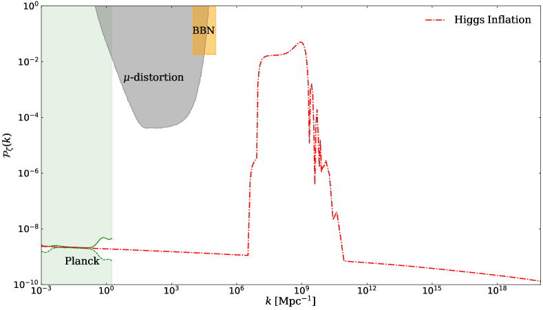
Figure 1: The power spectrum of curvature perturbations originates from the periodic structure of the Higgs inflation. The region shaded in light green is invalidated based on observations of the CMB Akrami et al. (2020). The orange and gray regions denote constraints originating from the impact on the neutron-to-proton ratio during primordial nucleosynthesis (BBN) Inomata et al. (2016); Jeong et al. (2014), and the $\mu$-distortion of the CMB Fixsen et al. (1996); Chluba et al. (2012), respectively.

By using the numerical results of the primordial curvature power spectrum, from the equation (22), we can obtain the energy density of the corresponding SIGWs, which is displayed in Figure 2 and denoted by the red line. The blue violins are the free spectrum constraints from the NANOGrav 15-yrs data set. Figure 2 shows that the energy density of the SIGWs from the Higgs inflation models can explain the NANOGrav 15-yrs data set.

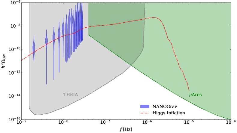
Figure 2: The red line is the energy density of SIGWs from the primordial curvature power spectrum displayed in Figure 1. The blue violins are the free spectrum constraints from the NANOGrav 15-yrs data set Agazie et al. (2023a); Afzal et al. (2023). The gray and green shaded areas are excluded by future observation experiments of THEIA The Theia Collaboration (2017) and µAres Sesana et al. (2021)

By using the PBH formulae and the numerical results of the primordial curvature power spectrum displayed in Figure 1, we can get the abundance of the PBH, and the results are displayed in Figure 3, represented by the red line. An interesting fact is that the corresponding abundance of the PBH is consistent with the implications of the ultrashort-timescale microlensing events recently observed by OGLE Mróz et al. (2017); Niikura et al. (2019a), as shown in Figure 3.

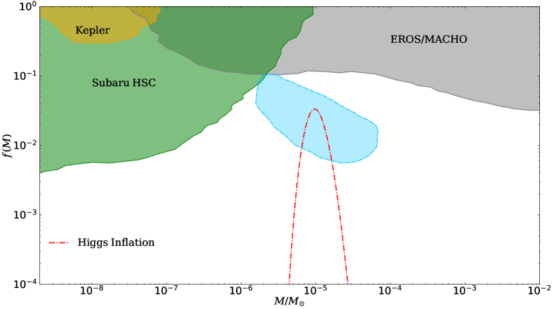
Figure 3: The red line is the abundance of the PBH from the primordial curvature power spectrum displayed in Figure 1. The shaded regions denote the main observational constraints on the PBH abundance: the gray region from the EROS/MACHO Tisserand et al. (2007), the green region from microlensing events with Subaru HSC Niikura et al. (2019b), and the orange region from the Kepler satellite Griest et al. (2013). The blue contour corresponds to the 95% confidence level representation of the PBH abundance, assuming that the six lensing objects of planetary mass identified in the OGLE Mróz et al. (2017) are PBHs Niikura et al. (2019a).

Summary and discussion. While the measurements obtained from the CMB and observations of large-scale structures have significantly improved our understanding of the Universe on a macroscopic level, our comprehension of smaller scales remains restricted, with the exception of the limitations imposed by PBHs. Conversely, PTAs serve as an indispensable instrument for investigating the state of the early Universe by means of SIGWs. The recently published data from the NANOGrav presents persuasive evidence in favor of the presence of a stochastic signal that corresponds to an SGWB. Our research demonstrates that this signal can be attributed to the SIGWs originating from the Higgs inflation model, specifically through the parametric amplification mechanism. Such an SGWB naturally predicts the substantial existence of planet-mass PBHs, which could potentially account for Planet 9 within our solar system Scholtz and Unwin (2020), as well as serve as the lensing objects responsible for the ultrashort-timescale microlensing events observed by the OGLE Mróz et al. (2017); Niikura et al. (2019a). The future observations of the SGWB through the utilization of PTAs and the study of planet-mass PBHs present an opportunity to offer additional confirmations on Higgs inflation, which unifies two fundamental aspects of theoretical physics, particle physics and cosmology. This framework could establish a connection between the microscopic world of particle interactions and the macroscopic evolution of the Universe.

The proposition that the SGWB at approximately $10^{-9}$ Hz and the planet-mass PBHs share the same origin is highly captivating, warranting further investigation through forthcoming experiments involving PTA, microlensing, and direct exploration for the existence of Planet 9. It is important to acknowledge that although the current observations on the SGWB and PBHs do not provide definitive evidence, future experiments hold the potential to elucidate both of these phenomena. The sensitivity of nanoHertz SGWB can be significantly enhanced by SKA Janssen et al. (2015), resulting in an increase of 3 to 5 orders of sensitivity. The utilization of Subaru HSC for microlensing search in the Andromeda Galaxy proves highly effective in mitigating the presence of unbounded planets, which predominantly reside in the galactic disk Niikura et al. (2019a); Kusenko et al. (2020). Moreover, the inclusion of a PBH with a mass of $10^{-5}~{}M_{\odot}$ within the solar system, referred to as Planet 9, has the potential to induce orbital irregularities in trans-Neptunian objects Scholtz and Unwin (2020). The investigation of its surrounding minihalo Siraj and Loeb (2020), Hawking radiation Arbey and Auffinger (2020), or gravitational field Witten (2020) could offer direct means to examine this phenomenon. Consequently, these experiments hold the potential to either verify or falsify the predictions made by our proposed scenario in the near future.

Acknowledgments ZY is supported by the National Natural Science Foundation of China under Grant No. 12205015 and the supporting fund for young researcher of Beijing Normal University under Grant No. 28719/310432102. ZQY is supported by the National Natural Science Foundation of China under Grant No. 12305059. ZCC is supported by the National Natural Science Foundation of China (Grant No. 12247176 and No. 12247112) and the China Postdoctoral Science Foundation Fellowship No. 2022M710429. LL is supported by the National Natural Science Foundation of China (Grant No. 12247112 and No. 12247176) and the China Postdoctoral Science Foundation Fellowship No. 2023M730300.

References

- Abbott et al. (2016a) B. P. Abbott et al. (LIGO Scientific, Virgo), “Observation of Gravitational Waves from a Binary Black Hole Merger,” Phys. Rev. Lett. 116, 061102 (2016a), arXiv:1602.03837 [gr-qc] .
- Abbott et al. (2016b) B. P. Abbott et al. (LIGO Scientific, Virgo), “GW151226: Observation of Gravitational Waves from a 22-Solar-Mass Binary Black Hole Coalescence,” Phys. Rev. Lett. 116, 241103 (2016b), arXiv:1606.04855 [gr-qc] .
- Abbott et al. (2017a) Benjamin P. Abbott et al. (LIGO Scientific, VIRGO), “GW170104: Observation of a 50-Solar-Mass Binary Black Hole Coalescence at Redshift 0.2,” Phys. Rev. Lett. 118, 221101 (2017a), [Erratum: Phys.Rev.Lett. 121, 129901 (2018)], arXiv:1706.01812 [gr-qc] .
- Abbott et al. (2017b) B. . P. . Abbott et al. (LIGO Scientific, Virgo), “GW170608: Observation of a 19-solar-mass Binary Black Hole Coalescence,” Astrophys. J. Lett. 851, L35 (2017b), arXiv:1711.05578 [astro-ph.HE] .
- Abbott et al. (2017c) B. P. Abbott et al. (LIGO Scientific, Virgo), “GW170814: A Three-Detector Observation of Gravitational Waves from a Binary Black Hole Coalescence,” Phys. Rev. Lett. 119, 141101 (2017c), arXiv:1709.09660 [gr-qc] .
- Abbott et al. (2017d) B. P. Abbott et al. (LIGO Scientific, Virgo), “GW170817: Observation of Gravitational Waves from a Binary Neutron Star Inspiral,” Phys. Rev. Lett. 119, 161101 (2017d), arXiv:1710.05832 [gr-qc] .
- Agazie et al. (2023a) Gabriella Agazie et al. (NANOGrav), “The NANOGrav 15 yr Data Set: Evidence for a Gravitational-wave Background,” Astrophys. J. Lett. 951, L8 (2023a), arXiv:2306.16213 [astro-ph.HE] .
- Agazie et al. (2023b) Gabriella Agazie et al. (NANOGrav), “The NANOGrav 15 yr Data Set: Observations and Timing of 68 Millisecond Pulsars,” Astrophys. J. Lett. 951, L9 (2023b), arXiv:2306.16217 [astro-ph.HE] .
- Zic et al. (2023) Andrew Zic et al., “The Parkes Pulsar Timing Array Third Data Release,” (2023), arXiv:2306.16230 [astro-ph.HE] .
- Reardon et al. (2023) Daniel J. Reardon et al., “Search for an Isotropic Gravitational-wave Background with the Parkes Pulsar Timing Array,” Astrophys. J. Lett. 951, L6 (2023), arXiv:2306.16215 [astro-ph.HE] .
- Antoniadis et al. (2023a) J. Antoniadis et al., “The second data release from the European Pulsar Timing Array I. The dataset and timing analysis,” (2023a), 10.1051/0004-6361/202346841, arXiv:2306.16224 [astro-ph.HE] .
- Antoniadis et al. (2023b) J. Antoniadis et al., “The second data release from the European Pulsar Timing Array III. Search for gravitational wave signals,” (2023b), arXiv:2306.16214 [astro-ph.HE] .
- Xu et al. (2023) Heng Xu et al., “Searching for the Nano-Hertz Stochastic Gravitational Wave Background with the Chinese Pulsar Timing Array Data Release I,” Res. Astron. Astrophys. 23, 075024 (2023), arXiv:2306.16216 [astro-ph.HE] .
- Hellings and Downs (1983) R. w. Hellings and G. s. Downs, “UPPER LIMITS ON THE ISOTROPIC GRAVITATIONAL RADIATION BACKGROUND FROM PULSAR TIMING ANALYSIS,” Astrophys. J. Lett. 265, L39–L42 (1983).
- Li et al. (2019) Jun Li, Zu-Cheng Chen, and Qing-Guo Huang, “Measuring the tilt of primordial gravitational-wave power spectrum from observations,” Sci. China Phys. Mech. Astron. 62, 110421 (2019), [Erratum: Sci.China Phys.Mech.Astron. 64, 250451 (2021)], arXiv:1907.09794 [astro-ph.CO] .
- Vagnozzi (2021) Sunny Vagnozzi, “Implications of the NANOGrav results for inflation,” Mon. Not. Roy. Astron. Soc. 502, L11–L15 (2021), arXiv:2009.13432 [astro-ph.CO] .
- Chen et al. (2021) Zu-Cheng Chen, Chen Yuan, and Qing-Guo Huang, “Non-tensorial gravitational wave background in NANOGrav 12.5-year data set,” Sci. China Phys. Mech. Astron. 64, 120412 (2021), arXiv:2101.06869 [astro-ph.CO] .
- Wu et al. (2022a) Yu-Mei Wu, Zu-Cheng Chen, and Qing-Guo Huang, “Constraining the Polarization of Gravitational Waves with the Parkes Pulsar Timing Array Second Data Release,” Astrophys. J. 925, 37 (2022a), arXiv:2108.10518 [astro-ph.CO] .
- Chen et al. (2022a) Zu-Cheng Chen, Yu-Mei Wu, and Qing-Guo Huang, “Searching for isotropic stochastic gravitational-wave background in the international pulsar timing array second data release,” Commun. Theor. Phys. 74, 105402 (2022a), arXiv:2109.00296 [astro-ph.CO] .
- Benetti et al. (2022) Micol Benetti, Leila Lobato Graef, and Sunny Vagnozzi, “Primordial gravitational waves from NANOGrav: A broken power-law approach,” Phys. Rev. D 105, 043520 (2022), arXiv:2111.04758 [astro-ph.CO] .
- Chen et al. (2022b) Zu-Cheng Chen, Yu-Mei Wu, and Qing-Guo Huang, “Search for the Gravitational-wave Background from Cosmic Strings with the Parkes Pulsar Timing Array Second Data Release,” Astrophys. J. 936, 20 (2022b), arXiv:2205.07194 [astro-ph.CO] .
- Ashoorioon et al. (2022) Amjad Ashoorioon, Kazem Rezazadeh, and Abasalt Rostami, “NANOGrav signal from the end of inflation and the LIGO mass and heavier primordial black holes,” Phys. Lett. B 835, 137542 (2022), arXiv:2202.01131 [astro-ph.CO] .
- Wu et al. (2022b) Yu-Mei Wu, Zu-Cheng Chen, Qing-Guo Huang, Xingjiang Zhu, N. D. Ramesh Bhat, Yi Feng, George Hobbs, Richard N. Manchester, Christopher J. Russell, and R. M. Shannon (PPTA), “Constraining ultralight vector dark matter with the Parkes Pulsar Timing Array second data release,” Phys. Rev. D 106, L081101 (2022b), arXiv:2210.03880 [astro-ph.CO] .
- Wu et al. (2023a) Yu-Mei Wu, Zu-Cheng Chen, and Qing-Guo Huang, “Search for stochastic gravitational-wave background from massive gravity in the NANOGrav 12.5-year dataset,” Phys. Rev. D 107, 042003 (2023a), arXiv:2302.00229 [gr-qc] .
- Falxa et al. (2023) M. Falxa et al. (IPTA), “Searching for continuous Gravitational Waves in the second data release of the International Pulsar Timing Array,” Mon. Not. Roy. Astron. Soc. 521, 5077–5086 (2023), arXiv:2303.10767 [gr-qc] .
- Wu et al. (2023b) Yu-Mei Wu, Zu-Cheng Chen, and Qing-Guo Huang, “Pulsar timing residual induced by ultralight tensor dark matter,” (2023b), arXiv:2305.08091 [hep-ph] .
- Dandoy et al. (2023) Virgile Dandoy, Valerie Domcke, and Fabrizio Rompineve, “Search for scalar induced gravitational waves in the International Pulsar Timing Array Data Release 2 and NANOgrav 12.5 years datasets,” (2023), arXiv:2302.07901 [astro-ph.CO] .
- Madge et al. (2023) Eric Madge, Enrico Morgante, Cristina Puchades Ibáñez, Nicklas Ramberg, and Sebastian Schenk, “Primordial gravitational waves in the nano-Hertz regime and PTA data – towards solving the GW inverse problem,” (2023), arXiv:2306.14856 [hep-ph] .
- Afzal et al. (2023) Adeela Afzal et al. (NANOGrav), “The NANOGrav 15 yr Data Set: Search for Signals from New Physics,” Astrophys. J. Lett. 951, L11 (2023), arXiv:2306.16219 [astro-ph.HE] .
- Antoniadis et al. (2023c) J. Antoniadis et al., “The second data release from the European Pulsar Timing Array: V. Implications for massive black holes, dark matter and the early Universe,” (2023c), arXiv:2306.16227 [astro-ph.CO] .
- King et al. (2023a) Stephen F. King, Danny Marfatia, and Moinul Hossain Rahat, “Towards distinguishing Dirac from Majorana neutrino mass with gravitational waves,” (2023a), arXiv:2306.05389 [hep-ph] .
- Niu and Rahat (2023) Xuce Niu and Moinul Hossain Rahat, “NANOGrav signal from axion inflation,” (2023), arXiv:2307.01192 [hep-ph] .
- Bi et al. (2023) Yan-Chen Bi, Yu-Mei Wu, Zu-Cheng Chen, and Qing-Guo Huang, “Implications for the Supermassive Black Hole Binaries from the NANOGrav 15-year Data Set,” (2023), arXiv:2307.00722 [astro-ph.CO] .
- Liu et al. (2023a) Lang Liu, Zu-Cheng Chen, and Qing-Guo Huang, “Probing the equation of state of the early Universe with pulsar timing arrays,” (2023a), arXiv:2307.14911 [astro-ph.CO] .
- Vagnozzi (2023) Sunny Vagnozzi, “Inflationary interpretation of the stochastic gravitational wave background signal detected by pulsar timing array experiments,” (2023), arXiv:2306.16912 [astro-ph.CO] .
- Han et al. (2023) Chengcheng Han, Ke-Pan Xie, Jin Min Yang, and Mengchao Zhang, “Self-interacting dark matter implied by nano-Hertz gravitational waves,” (2023), arXiv:2306.16966 [hep-ph] .
- Li et al. (2023) Yaoyu Li, Chi Zhang, Ziwei Wang, Mingyang Cui, Yue-Lin Sming Tsai, Qiang Yuan, and Yi-Zhong Fan, “Primordial magnetic field as a common solution of nanohertz gravitational waves and Hubble tension,” (2023), arXiv:2306.17124 [astro-ph.HE] .
- Franciolini et al. (2023a) Gabriele Franciolini, Davide Racco, and Fabrizio Rompineve, “Footprints of the QCD Crossover on Cosmological Gravitational Waves at Pulsar Timing Arrays,” (2023a), arXiv:2306.17136 [astro-ph.CO] .
- Shen et al. (2023) Zhao-Qiang Shen, Guan-Wen Yuan, Yi-Ying Wang, and Yuan-Zhu Wang, “Dark Matter Spike surrounding Supermassive Black Holes Binary and the nanohertz Stochastic Gravitational Wave Background,” (2023), arXiv:2306.17143 [astro-ph.HE] .
- Kitajima et al. (2023) Naoya Kitajima, Junseok Lee, Kai Murai, Fuminobu Takahashi, and Wen Yin, “Nanohertz Gravitational Waves from Axion Domain Walls Coupled to QCD,” (2023), arXiv:2306.17146 [hep-ph] .
- Franciolini et al. (2023b) Gabriele Franciolini, Antonio Iovino, Junior., Ville Vaskonen, and Hardi Veermae, “The recent gravitational wave observation by pulsar timing arrays and primordial black holes: the importance of non-gaussianities,” (2023b), arXiv:2306.17149 [astro-ph.CO] .
- Addazi et al. (2023) Andrea Addazi, Yi-Fu Cai, Antonino Marciano, and Luca Visinelli, “Have pulsar timing array methods detected a cosmological phase transition?” (2023), arXiv:2306.17205 [astro-ph.CO] .
- Cai et al. (2023) Yi-Fu Cai, Xin-Chen He, Xiaohan Ma, Sheng-Feng Yan, and Guan-Wen Yuan, “Limits on scalar-induced gravitational waves from the stochastic background by pulsar timing array observations,” (2023), arXiv:2306.17822 [gr-qc] .
- Inomata et al. (2023) Keisuke Inomata, Kazunori Kohri, and Takahiro Terada, “The Detected Stochastic Gravitational Waves and Sub-Solar Primordial Black Holes,” (2023), arXiv:2306.17834 [astro-ph.CO] .
- Wang et al. (2023) Sai Wang, Zhi-Chao Zhao, Jun-Peng Li, and Qing-Hua Zhu, “Exploring the Implications of 2023 Pulsar Timing Array Datasets for Scalar-Induced Gravitational Waves and Primordial Black Holes,” (2023), arXiv:2307.00572 [astro-ph.CO] .
- Murai and Yin (2023) Kai Murai and Wen Yin, “A Novel Probe of Supersymmetry in Light of Nanohertz Gravitational Waves,” (2023), arXiv:2307.00628 [hep-ph] .
- Li and Xie (2023) Shao-Ping Li and Ke-Pan Xie, “A collider test of nano-Hertz gravitational waves from pulsar timing arrays,” (2023), arXiv:2307.01086 [hep-ph] .
- Anchordoqui et al. (2023) Luis A. Anchordoqui, Ignatios Antoniadis, and Dieter Lust, “Fuzzy Dark Matter, the Dark Dimension, and the Pulsar Timing Array Signal,” (2023), arXiv:2307.01100 [hep-ph] .
- Liu et al. (2023b) Lang Liu, Zu-Cheng Chen, and Qing-Guo Huang, “Implications for the non-Gaussianity of curvature perturbation from pulsar timing arrays,” (2023b), arXiv:2307.01102 [astro-ph.CO] .
- Zhu et al. (2023) Qing-Hua Zhu, Zhi-Chao Zhao, and Sai Wang, “Joint implications of BBN, CMB, and PTA Datasets for Scalar-Induced Gravitational Waves of Second and Third orders,” (2023), arXiv:2307.03095 [astro-ph.CO] .
- Abe and Tada (2023) Katsuya T. Abe and Yuichiro Tada, “Translating nano-Hertz gravitational wave background into primordial perturbations taking account of the cosmological QCD phase transition,” (2023), arXiv:2307.01653 [astro-ph.CO] .
- Ghosh et al. (2023) Tathagata Ghosh, Anish Ghoshal, Huai-Ke Guo, Fazlollah Hajkarim, Stephen F. King, Kuver Sinha, Xin Wang, and Graham White, “Did we hear the sound of the Universe boiling? Analysis using the full fluid velocity profiles and NANOGrav 15-year data,” (2023), arXiv:2307.02259 [astro-ph.HE] .
- Figueroa et al. (2023) Daniel G. Figueroa, Mauro Pieroni, Angelo Ricciardone, and Peera Simakachorn, “Cosmological Background Interpretation of Pulsar Timing Array Data,” (2023), arXiv:2307.02399 [astro-ph.CO] .
- Yi et al. (2023a) Zhu Yi, Qing Gao, Yungui Gong, Yue Wang, and Fengge Zhang, “The waveform of the scalar induced gravitational waves in light of Pulsar Timing Array data,” (2023a), arXiv:2307.02467 [gr-qc] .
- Wu et al. (2023c) Yu-Mei Wu, Zu-Cheng Chen, and Qing-Guo Huang, “Cosmological Interpretation for the Stochastic Signal in Pulsar Timing Arrays,” (2023c), arXiv:2307.03141 [astro-ph.CO] .
- Li (2023) Xiu-Fei Li, “Probing the high temperature symmetry breaking with gravitational waves from domain walls,” (2023), arXiv:2307.03163 [hep-ph] .
- Geller et al. (2023) Michael Geller, Subhajit Ghosh, Sida Lu, and Yuhsin Tsai, “Challenges in Interpreting the NANOGrav 15-Year Data Set as Early Universe Gravitational Waves Produced by ALP Induced Instability,” (2023), arXiv:2307.03724 [hep-ph] .
- You et al. (2023) Zhi-Qiang You, Zhu Yi, and You Wu, “Constraints on primordial curvature power spectrum with pulsar timing arrays,” (2023), arXiv:2307.04419 [gr-qc] .
- Antusch et al. (2023) Stefan Antusch, Kevin Hinze, Shaikh Saad, and Jonathan Steiner, “Singling out SO(10) GUT models using recent PTA results,” (2023), arXiv:2307.04595 [hep-ph] .
- Ye and Silvestri (2023) Gen Ye and Alessandra Silvestri, “Can gravitational wave background feel wiggles in spacetime?” (2023), arXiv:2307.05455 [astro-ph.CO] .
- Hosseini Mansoori et al. (2023) Seyed Ali Hosseini Mansoori, Fereshteh Felegray, Alireza Talebian, and Mohammad Sami, “PBHs and GWs from -inflation and NANOGrav 15-year data,” (2023), arXiv:2307.06757 [astro-ph.CO] .
- Jin et al. (2023) Jia-Heng Jin, Zu-Cheng Chen, Zhu Yi, Zhi-Qiang You, Lang Liu, and You Wu, “Confronting sound speed resonance with pulsar timing arrays,” (2023), arXiv:2307.08687 [astro-ph.CO] .
- Zhang et al. (2023) Zhao Zhang, Chengfeng Cai, Yu-Hang Su, Shiyu Wang, Zhao-Huan Yu, and Hong-Hao Zhang, “Nano-Hertz gravitational waves from collapsing domain walls associated with freeze-in dark matter in light of pulsar timing array observations,” (2023), arXiv:2307.11495 [hep-ph] .
- Valbusa Dall’Armi et al. (2023) Lorenzo Valbusa Dall’Armi, Alina Mierna, Sabino Matarrese, and Angelo Ricciardone, “Adiabatic or Non-Adiabatic? Unraveling the Nature of Initial Conditions in the Cosmological Gravitational Wave Background,” (2023), arXiv:2307.11043 [astro-ph.CO] .
- De Luca et al. (2023) Valerio De Luca, Alex Kehagias, and Antonio Riotto, “How Well Do We Know the Primordial Black Hole Abundance? The Crucial Role of Non-Linearities when Approaching the Horizon,” (2023), arXiv:2307.13633 [astro-ph.CO] .
- Gorji et al. (2023) Mohammad Ali Gorji, Misao Sasaki, and Teruaki Suyama, “Extra-tensor-induced origin for the PTA signal: No primordial black hole production,” (2023), arXiv:2307.13109 [astro-ph.CO] .
- Das et al. (2023) Barnali Das, Nur Jaman, and M. Sami, “Gravitational Waves Background (NANOGrav) from Quintessential Inflation,” (2023), arXiv:2307.12913 [gr-qc] .
- Yi et al. (2023b) Zhu Yi, Zhi-Qiang You, and You Wu, “Model-independent reconstruction of the primordial curvature power spectrum from PTA data,” (2023b), arXiv:2308.05632 [astro-ph.CO] .
- Ellis et al. (2023) John Ellis, Malcolm Fairbairn, Gabriele Franciolini, Gert Hütsi, Antonio Iovino, Marek Lewicki, Martti Raidal, Juan Urrutia, Ville Vaskonen, and Hardi Veermäe, “What is the source of the PTA GW signal?” (2023), arXiv:2308.08546 [astro-ph.CO] .
- He et al. (2023) Song He, Li Li, Sai Wang, and Shao-Jiang Wang, “Constraints on holographic QCD phase transitions from PTA observations,” (2023), arXiv:2308.07257 [hep-ph] .
- Zhao et al. (2023) Zhi-Chao Zhao, Qing-Hua Zhu, Sai Wang, and Xin Zhang, “Exploring the Equation of State of the Early Universe: Insights from BBN, CMB, and PTA Observations,” (2023), arXiv:2307.13574 [astro-ph.CO] .
- Balaji et al. (2023) Shyam Balaji, Guillem Domènech, and Gabriele Franciolini, “Scalar-induced gravitational wave interpretation of PTA data: the role of scalar fluctuation propagation speed,” (2023), arXiv:2307.08552 [gr-qc] .
- Kawasaki and Murai (2023) Masahiro Kawasaki and Kai Murai, “Enhancement of gravitational waves at Q-ball decay including non-linear density perturbations,” (2023), arXiv:2308.13134 [astro-ph.CO] .
- Cannizzaro et al. (2023) Enrico Cannizzaro, Gabriele Franciolini, and Paolo Pani, “Novel tests of gravity using nano-Hertz stochastic gravitational-wave background signals,” (2023), arXiv:2307.11665 [gr-qc] .
- King et al. (2023b) Stephen F. King, Rishav Roshan, Xin Wang, Graham White, and Masahito Yamazaki, “Quantum Gravity Effects on Dark Matter and Gravitational Waves,” (2023b), arXiv:2308.03724 [hep-ph] .
- Maji and Park (2023) Rinku Maji and Wan-Il Park, “Supersymmetric flat direction and NANOGrav 15 year data,” (2023), arXiv:2308.11439 [hep-ph] .
- Bhaumik et al. (2023) Nilanjandev Bhaumik, Rajeev Kumar Jain, and Marek Lewicki, “Ultra-low mass PBHs in the early universe can explain the PTA signal,” (2023), arXiv:2308.07912 [astro-ph.CO] .
- Zel’dovich and Novikov (1967) Ya. B. Zel’dovich and I. D. Novikov, “The Hypothesis of Cores Retarded during Expansion and the Hot Cosmological Model,” Soviet Astron. AJ (Engl. Transl. ), 10, 602 (1967).
- Hawking (1971) Stephen Hawking, “Gravitationally collapsed objects of very low mass,” Mon. Not. Roy. Astron. Soc. 152, 75 (1971).
- Carr and Hawking (1974) Bernard J. Carr and S. W. Hawking, “Black holes in the early Universe,” Mon. Not. Roy. Astron. Soc. 168, 399–415 (1974).
- Belotsky et al. (2014) K. M. Belotsky, A. D. Dmitriev, E. A. Esipova, V. A. Gani, A. V. Grobov, M. Yu. Khlopov, A. A. Kirillov, S. G. Rubin, and I. V. Svadkovsky, “Signatures of primordial black hole dark matter,” Mod. Phys. Lett. A 29, 1440005 (2014), arXiv:1410.0203 [astro-ph.CO] .
- Carr et al. (2016) Bernard Carr, Florian Kuhnel, and Marit Sandstad, “Primordial Black Holes as Dark Matter,” Phys. Rev. D 94, 083504 (2016), arXiv:1607.06077 [astro-ph.CO] .
- Garcia-Bellido and Ruiz Morales (2017) Juan Garcia-Bellido and Ester Ruiz Morales, “Primordial black holes from single field models of inflation,” Phys. Dark Univ. 18, 47–54 (2017), arXiv:1702.03901 [astro-ph.CO] .
- Carr et al. (2017) Bernard Carr, Martti Raidal, Tommi Tenkanen, Ville Vaskonen, and Hardi Veermäe, “Primordial black hole constraints for extended mass functions,” Phys. Rev. D 96, 023514 (2017), arXiv:1705.05567 [astro-ph.CO] .
- Germani and Prokopec (2017) Cristiano Germani and Tomislav Prokopec, “On primordial black holes from an inflection point,” Phys. Dark Univ. 18, 6–10 (2017), arXiv:1706.04226 [astro-ph.CO] .
- Chen et al. (2019) Zu-Cheng Chen, Fan Huang, and Qing-Guo Huang, “Stochastic Gravitational-wave Background from Binary Black Holes and Binary Neutron Stars and Implications for LISA,” Astrophys. J. 871, 97 (2019), arXiv:1809.10360 [gr-qc] .
- Liu et al. (2019a) Lang Liu, Zong-Kuan Guo, and Rong-Gen Cai, “Effects of the surrounding primordial black holes on the merger rate of primordial black hole binaries,” Phys. Rev. D 99, 063523 (2019a), arXiv:1812.05376 [astro-ph.CO] .
- Chen and Huang (2018) Zu-Cheng Chen and Qing-Guo Huang, “Merger Rate Distribution of Primordial-Black-Hole Binaries,” Astrophys. J. 864, 61 (2018), arXiv:1801.10327 [astro-ph.CO] .
- Cai et al. (2019) Rong-gen Cai, Shi Pi, and Misao Sasaki, “Gravitational Waves Induced by non-Gaussian Scalar Perturbations,” Phys. Rev. Lett. 122, 201101 (2019), arXiv:1810.11000 [astro-ph.CO] .
- Liu et al. (2019b) Lang Liu, Zong-Kuan Guo, and Rong-Gen Cai, “Effects of the merger history on the merger rate density of primordial black hole binaries,” Eur. Phys. J. C 79, 717 (2019b), arXiv:1901.07672 [astro-ph.CO] .
- Fu et al. (2019) Chengjie Fu, Puxun Wu, and Hongwei Yu, “Primordial Black Holes from Inflation with Nonminimal Derivative Coupling,” Phys. Rev. D 100, 063532 (2019), arXiv:1907.05042 [astro-ph.CO] .
- Liu et al. (2020a) Jing Liu, Zong-Kuan Guo, and Rong-Gen Cai, “Primordial Black Holes from Cosmic Domain Walls,” Phys. Rev. D 101, 023513 (2020a), arXiv:1908.02662 [astro-ph.CO] .
- Cai et al. (2020) Rong-Gen Cai, Zong-Kuan Guo, Jing Liu, Lang Liu, and Xing-Yu Yang, “Primordial black holes and gravitational waves from parametric amplification of curvature perturbations,” JCAP 06, 013 (2020), arXiv:1912.10437 [astro-ph.CO] .
- Chen and Huang (2020) Zu-Cheng Chen and Qing-Guo Huang, “Distinguishing Primordial Black Holes from Astrophysical Black Holes by Einstein Telescope and Cosmic Explorer,” JCAP 08, 039 (2020), arXiv:1904.02396 [astro-ph.CO] .
- Liu et al. (2020b) Lang Liu, Zong-Kuan Guo, Rong-Gen Cai, and Sang Pyo Kim, “Merger rate distribution of primordial black hole binaries with electric charges,” Phys. Rev. D 102, 043508 (2020b), arXiv:2001.02984 [astro-ph.CO] .
- Fu et al. (2020) Chengjie Fu, Puxun Wu, and Hongwei Yu, “Primordial black holes and oscillating gravitational waves in slow-roll and slow-climb inflation with an intermediate noninflationary phase,” Phys. Rev. D 102, 043527 (2020), arXiv:2006.03768 [astro-ph.CO] .
- De Luca et al. (2021a) V. De Luca, V. Desjacques, G. Franciolini, P. Pani, and A. Riotto, “GW190521 Mass Gap Event and the Primordial Black Hole Scenario,” Phys. Rev. Lett. 126, 051101 (2021a), arXiv:2009.01728 [astro-ph.CO] .
- Vaskonen and Veermäe (2021) Ville Vaskonen and Hardi Veermäe, “Did NANOGrav see a signal from primordial black hole formation?” Phys. Rev. Lett. 126, 051303 (2021), arXiv:2009.07832 [astro-ph.CO] .
- De Luca et al. (2021b) V. De Luca, G. Franciolini, and A. Riotto, “NANOGrav Data Hints at Primordial Black Holes as Dark Matter,” Phys. Rev. Lett. 126, 041303 (2021b), arXiv:2009.08268 [astro-ph.CO] .
- Domènech and Pi (2022) Guillem Domènech and Shi Pi, “NANOGrav hints on planet-mass primordial black holes,” Sci. China Phys. Mech. Astron. 65, 230411 (2022), arXiv:2010.03976 [astro-ph.CO] .
- Hütsi et al. (2021) Gert Hütsi, Martti Raidal, Ville Vaskonen, and Hardi Veermäe, “Two populations of LIGO-Virgo black holes,” JCAP 03, 068 (2021), arXiv:2012.02786 [astro-ph.CO] .
- Chen et al. (2022c) Zu-Cheng Chen, Chen Yuan, and Qing-Guo Huang, “Confronting the primordial black hole scenario with the gravitational-wave events detected by LIGO-Virgo,” Phys. Lett. B 829, 137040 (2022c), arXiv:2108.11740 [astro-ph.CO] .
- Kawai and Kim (2021) Shinsuke Kawai and Jinsu Kim, “Primordial black holes from Gauss-Bonnet-corrected single field inflation,” Phys. Rev. D 104, 083545 (2021), arXiv:2108.01340 [astro-ph.CO] .
- Braglia et al. (2021) Matteo Braglia, Juan Garcia-Bellido, and Sachiko Kuroyanagi, “Testing Primordial Black Holes with multi-band observations of the stochastic gravitational wave background,” JCAP 12, 012 (2021), arXiv:2110.07488 [astro-ph.CO] .
- Liu et al. (2023c) Lang Liu, Xing-Yu Yang, Zong-Kuan Guo, and Rong-Gen Cai, “Testing primordial black hole and measuring the Hubble constant with multiband gravitational-wave observations,” JCAP 01, 006 (2023c), arXiv:2112.05473 [astro-ph.CO] .
- Braglia et al. (2023) Matteo Braglia, Juan Garcia-Bellido, and Sachiko Kuroyanagi, “Tracking the origin of black holes with the stochastic gravitational wave background popcorn signal,” Mon. Not. Roy. Astron. Soc. 519, 6008–6019 (2023), arXiv:2201.13414 [astro-ph.CO] .
- Zheng et al. (2023) Li-Ming Zheng, Zhengxiang Li, Zu-Cheng Chen, Huan Zhou, and Zong-Hong Zhu, “Towards a reliable reconstruction of the power spectrum of primordial curvature perturbation on small scales from GWTC-3,” Phys. Lett. B 838, 137720 (2023), arXiv:2212.05516 [astro-ph.CO] .
- Liu et al. (2023d) Lang Liu, Zhi-Qiang You, You Wu, and Zu-Cheng Chen, “Constraining the merger history of primordial-black-hole binaries from GWTC-3,” Phys. Rev. D 107, 063035 (2023d), arXiv:2210.16094 [astro-ph.CO] .
- Chen et al. (2023) Zu-Cheng Chen, Shen-Shi Du, Qing-Guo Huang, and Zhi-Qiang You, “Constraints on primordial-black-hole population and cosmic expansion history from GWTC-3,” JCAP 03, 024 (2023), arXiv:2205.11278 [astro-ph.CO] .
- Guo et al. (2023) Shu-Yuan Guo, Maxim Khlopov, Xuewen Liu, Lei Wu, Yongcheng Wu, and Bin Zhu, “Footprints of Axion-Like Particle in Pulsar Timing Array Data and JWST Observations,” (2023), arXiv:2306.17022 [hep-ph] .
- Sasaki et al. (2018) Misao Sasaki, Teruaki Suyama, Takahiro Tanaka, and Shuichiro Yokoyama, “Primordial black holes—perspectives in gravitational wave astronomy,” Class. Quant. Grav. 35, 063001 (2018), arXiv:1801.05235 [astro-ph.CO] .
- Carr et al. (2021) Bernard Carr, Kazunori Kohri, Yuuiti Sendouda, and Jun’ichi Yokoyama, “Constraints on primordial black holes,” Rept. Prog. Phys. 84, 116902 (2021), arXiv:2002.12778 [astro-ph.CO] .
- Carr and Kuhnel (2020) Bernard Carr and Florian Kuhnel, “Primordial Black Holes as Dark Matter: Recent Developments,” Ann. Rev. Nucl. Part. Sci. 70, 355–394 (2020), arXiv:2006.02838 [astro-ph.CO] .
- Bird et al. (2016) Simeon Bird, Ilias Cholis, Julian B. Muñoz, Yacine Ali-Haïmoud, Marc Kamionkowski, Ely D. Kovetz, Alvise Raccanelli, and Adam G. Riess, “Did LIGO detect dark matter?” Phys. Rev. Lett. 116, 201301 (2016), arXiv:1603.00464 [astro-ph.CO] .
- Sasaki et al. (2016) Misao Sasaki, Teruaki Suyama, Takahiro Tanaka, and Shuichiro Yokoyama, “Primordial Black Hole Scenario for the Gravitational-Wave Event GW150914,” Phys. Rev. Lett. 117, 061101 (2016), [Erratum: Phys.Rev.Lett. 121, 059901 (2018)], arXiv:1603.08338 [astro-ph.CO] .
- Scholtz and Unwin (2020) Jakub Scholtz and James Unwin, “What if Planet 9 is a Primordial Black Hole?” Phys. Rev. Lett. 125, 051103 (2020), arXiv:1909.11090 [hep-ph] .
- Mróz et al. (2017) Przemek Mróz, Andrzej Udalski, Jan Skowron, Radosław Poleski, Szymon Kozłowski, Michał K. Szymański, Igor Soszyński, Łukasz Wyrzykowski, Paweł Pietrukowicz, Krzysztof Ulaczyk, Dorota Skowron, and Michał Pawlak, “No large population of unbound or wide-orbit jupiter-mass planets,” Nature 548, 183–186 (2017), arXiv:1707.07634 [astro-ph.EP] .
- Niikura et al. (2019a) Hiroko Niikura, Masahiro Takada, Shuichiro Yokoyama, Takahiro Sumi, and Shogo Masaki, “Constraints on Earth-mass primordial black holes from OGLE 5-year microlensing events,” Phys. Rev. D 99, 083503 (2019a), arXiv:1901.07120 [astro-ph.CO] .
- Kodama and Sasaki (1984) Hideo Kodama and Misao Sasaki, “Cosmological Perturbation Theory,” Prog. Theor. Phys. Suppl. 78, 1–166 (1984).
- Mukhanov et al. (1992) Viatcheslav F. Mukhanov, H. A. Feldman, and Robert H. Brandenberger, “Theory of cosmological perturbations. Part 1. Classical perturbations. Part 2. Quantum theory of perturbations. Part 3. Extensions,” Phys. Rept. 215, 203–333 (1992).
- Bezrukov and Shaposhnikov (2008) Fedor L. Bezrukov and Mikhail Shaposhnikov, “The Standard Model Higgs boson as the inflaton,” Phys. Lett. B 659, 703–706 (2008), arXiv:0710.3755 [hep-th] .
- Hwang (1997) Jai-chan Hwang, “Quantum fluctuations of cosmological perturbations in generalized gravity,” Class. Quant. Grav. 14, 3327–3336 (1997), arXiv:gr-qc/9607059 .
- Baumann et al. (2007) Daniel Baumann, Paul J. Steinhardt, Keitaro Takahashi, and Kiyotomo Ichiki, “Gravitational Wave Spectrum Induced by Primordial Scalar Perturbations,” Phys. Rev. D 76, 084019 (2007), arXiv:hep-th/0703290 .
- Weinberg (2004) Steven Weinberg, “Damping of tensor modes in cosmology,” Phys. Rev. D 69, 023503 (2004), arXiv:astro-ph/0306304 .
- Watanabe and Komatsu (2006) Yuki Watanabe and Eiichiro Komatsu, “Improved Calculation of the Primordial Gravitational Wave Spectrum in the Standard Model,” Phys. Rev. D 73, 123515 (2006), arXiv:astro-ph/0604176 .
- Kohri and Terada (2018) Kazunori Kohri and Takahiro Terada, “Semianalytic calculation of gravitational wave spectrum nonlinearly induced from primordial curvature perturbations,” Phys. Rev. D 97, 123532 (2018), arXiv:1804.08577 [gr-qc] .
- Espinosa et al. (2018) José Ramón Espinosa, Davide Racco, and Antonio Riotto, “A Cosmological Signature of the SM Higgs Instability: Gravitational Waves,” JCAP 09, 012 (2018), arXiv:1804.07732 [hep-ph] .
- Inomata et al. (2018) Keisuke Inomata, Masahiro Kawasaki, Kyohei Mukaida, and Tsutomu T. Yanagida, “Double inflation as a single origin of primordial black holes for all dark matter and LIGO observations,” Phys. Rev. D 97, 043514 (2018), arXiv:1711.06129 [astro-ph.CO] .
- Akrami et al. (2020) Y. Akrami et al. (Planck), “Planck 2018 results. X. Constraints on inflation,” Astron. Astrophys. 641, A10 (2020), arXiv:1807.06211 [astro-ph.CO] .
- Inomata et al. (2016) Keisuke Inomata, Masahiro Kawasaki, and Yuichiro Tada, “Revisiting constraints on small scale perturbations from big-bang nucleosynthesis,” Phys. Rev. D 94, 043527 (2016), arXiv:1605.04646 [astro-ph.CO] .
- Jeong et al. (2014) Donghui Jeong, Josef Pradler, Jens Chluba, and Marc Kamionkowski, “Silk damping at a redshift of a billion: a new limit on small-scale adiabatic perturbations,” Phys. Rev. Lett. 113, 061301 (2014), arXiv:1403.3697 [astro-ph.CO] .
- Fixsen et al. (1996) D. J. Fixsen, E. S. Cheng, J. M. Gales, John C. Mather, R. A. Shafer, and E. L. Wright, “The Cosmic Microwave Background spectrum from the full COBE FIRAS data set,” Astrophys. J. 473, 576 (1996), arXiv:astro-ph/9605054 .
- Chluba et al. (2012) Jens Chluba, Adrienne L. Erickcek, and Ido Ben-Dayan, “Probing the inflaton: Small-scale power spectrum constraints from measurements of the CMB energy spectrum,” Astrophys. J. 758, 76 (2012), arXiv:1203.2681 [astro-ph.CO] .
- The Theia Collaboration (2017) The Theia Collaboration, “Theia: Faint objects in motion or the new astrometry frontier,” arXiv e-prints , arXiv:1707.01348 (2017), arXiv:1707.01348 [astro-ph.IM] .
- Sesana et al. (2021) Alberto Sesana et al., “Unveiling the gravitational universe at -Hz frequencies,” Exper. Astron. 51, 1333–1383 (2021), arXiv:1908.11391 [astro-ph.IM] .
- Tisserand et al. (2007) P. Tisserand et al. (EROS-2), “Limits on the macho content of the galactic halo from the eros-2 survey of the magellanic clouds,” Astron. Astrophys. 469, 387–404 (2007), arXiv:astro-ph/0607207 .
- Niikura et al. (2019b) Hiroko Niikura et al., “Microlensing constraints on primordial black holes with Subaru/HSC Andromeda observations,” Nature Astron. 3, 524–534 (2019b), arXiv:1701.02151 [astro-ph.CO] .
- Griest et al. (2013) Kim Griest, Agnieszka M. Cieplak, and Matthew J. Lehner, “New Limits on Primordial Black Hole Dark Matter from an Analysis of Kepler Source Microlensing Data,” Phys. Rev. Lett. 111, 181302 (2013).
- Janssen et al. (2015) Gemma Janssen et al., “Gravitational wave astronomy with the SKA,” PoS AASKA14, 037 (2015), arXiv:1501.00127 [astro-ph.IM] .
- Kusenko et al. (2020) Alexander Kusenko, Misao Sasaki, Sunao Sugiyama, Masahiro Takada, Volodymyr Takhistov, and Edoardo Vitagliano, “Exploring Primordial Black Holes from the Multiverse with Optical Telescopes,” Phys. Rev. Lett. 125, 181304 (2020), arXiv:2001.09160 [astro-ph.CO] .
- Siraj and Loeb (2020) Amir Siraj and Abraham Loeb, “Searching for Black Holes in the Outer Solar System with LSST,” Astrophys. J. Lett. 898, L4 (2020), arXiv:2005.12280 [astro-ph.HE] .
- Arbey and Auffinger (2020) Alexandre Arbey and Jérémy Auffinger, “Detecting Planet 9 via Hawking radiation,” (2020), arXiv:2006.02944 [gr-qc] .
- Witten (2020) Edward Witten, “Searching for a Black Hole in the Outer Solar System,” (2020), arXiv:2004.14192 [astro-ph.EP] .