Scalable Algorithms for calculating Power Function of Random Quantum States in NISQ Era

Abstract

This article focuses on the development of scalable and quantum bit-efficient algorithms for computing power functions of random quantum states. Two algorithms, based on Hadamard testing and Gate Set Tomography, are proposed. We provide a comparative analysis of their computational outcomes, accompanied by a meticulous evaluation of inherent errors in the gate set tomography approach. The second algorithm exhibits a significant reduction in the utilization of two-qubit gates compared to the first. As an illustration, we apply both methods to compute the Von Neumann entropy of randomly generated quantum states.

I Introduction

Random quantum states form the foundational basis for our understanding of Quantum Informationswingle2016measuring; brandao2021models, Black holeshayden2007black; kudler2021relative, and related fields. Numerous important functions, such as Renyi entropy, Von Neumann entropy, Quantum Fisher information, fidelity of random states, virtual distillation, and separation of density matricesholmes2023nonlinear; subramanian2021quantum; zyczkowski2006introduction; rath2021quantum; jozsa1994fidelity; koczor2021exponential; wang2022new, play crucial roles in quantum information, condensed matter physics, quantum chemistry, and beyondkandala2017hardware; carteret2005noiseless; lubasch2020variational; georgeot2001exponential; elben2020many; braumuller2022probing. Quantum computing holds a significant computational efficiency advantage over classical computingnational2019quantum. The current development of quantum devices is situated in the Noisy Intermediate-Scale Quantum (NISQ) era, characterized by the handling of qubits in the tens or hundreds, accompanied by inevitable quantum noisepreskill2018quantum; lau2022nisq; ding2022quantum. Exploiting the advantages and addressing the challenges of NISQ quantum computers, we tackle the fundamental yet challenging task of developing algorithms for computing nonlinear functions of random quantum state.

Prior methodologies for nonlinear transformations relied on simultaneously preparing multiple copies of a quantum statezhou2022hybrid; holmes2023nonlinear; bovino2005direct; horodecki2003measuring; ekert2002direct and collective measurementsbovino2005direct; ekert2002direct; horodecki2003measuring. These approaches necessitated a large number of qubits. For instance, when computing $\mathrm{Tr}\{\rho^{m}\}$, with $\rho$ representing the density matrix defined over $n$ qubits, these methods required $nm$ qubits. However, in the NISQ era, the number of qubits is still insufficient, rendering it inadequate to achieve quantum advantage within these algorithmspreskill2018quantum. Conversely, researchers have advocated for constructing the classical shadow of $\rho$ and subsequently employing it to compute the purity $\mathrm{Tr}\{\rho^{2}\}$sack2022avoiding; zhang2021experimental; seif2023shadow; elben2023randomized; brydges2019probing; elben2019statistical; elben2020mixed. While this approach still entails exponential resources relative to the number of qubits, it is perceived as an improvement over traditional State Tomographyo2016efficient. Nevertheless, ongoing exploration of such methods is delimited to purity, which corresponds to quadratic functions of the density matrix. For higher-order functions like $\mathrm{Tr}\{\rho^{m}\}$, there is no verified indication that these methods sustain an advantage over classical approaches.

To more efficiently exploit quantum computers in the NISQ era, we aim to design algorithms that employ the same number of qubits as $\rho$, and the circuit depth exhibits polynomial growth with the order of nonlinear function. A technique for generating random states involves initiating from an initial state and applying quantum gates randomly based on a specific probability distribution. The resultant final states post the application of diverse quantum gates to the initial state might not be orthogonal. We ascertain the presence of the algorithm we want, assuming the knowledge about how to construct the intended random state by utilizing random circuits.

In this study, we introduce two distinct algorithms, both characterized by their shared utilization of the Grover gate $G=I-2|0\rangle\langle 0|$. The primary aim of both algorithms is to compute the power series expansion $\mathrm{Tr}\{\rho^{m}\}$ for a nonlinear function in the context of a multi-qubit quantum random state $\rho$. The first algorithm is based on the Hadamard Test(HT). It involves transforming an auxiliary qubit (usually $|0\rangle\langle 0|$) into a superposition state using the Hadamard gate. After a controlled gate operation, another Hadamard gate extracts essential data, finalizing the calculation. Our algorithm is Hadamard Test-based but introduces an innovative approach: we deploy a quantum pure state circuit to simulate $\mathrm{Tr}\{G^{m-1}\rho\}$ computation for a quantum random state, by employing weighted averages across multiple measurements. The second algorithm begins by mathematically converting the calculation of $\mathrm{Tr}\{\rho^{m}\}$ for the desired quantum state into $\mathrm{Tr}\{G^{m}\}$. A comprehensive understanding of $G^{m}$ is acquired through Gate Set Tomography(GST)d2003quantum; yang2021perturbative in a subspace, facilitating the calculation and estimation of $\mathrm{Tr}\{G^{m}\}$ through mathematical processing. Compared to the Hadamard Test-based algorithm, this approach entails fewer qubits and two-qubit gates within the circuit. Moreover, this method introduces a novel result-processing technique rooted in reconstruction. Both of these algorithms are scalable, with their time complexity growing polynomially with the number of qubits.

The structure of this paper is outlined as follows. We begin by introducing the Hadamard test-based algorithm in Section II. Subsequently, we explain the application of the GST method in Section III for extracting relevant information from the subspace. Section LABEL:Error_Analysis is devoted to error analysis and complexities. In Section LABEL:results-and-discussion, we present computational results garnered from the preparation of the random quantum state $\rho$ and the subsequent application of both algorithms. Notably, we compare the variations in calculations for the identical quantum state when utilizing the two distinct algorithms. A concise summary of this article is offered in Section LABEL:conclusion.

In the appendix, we explore into specific scenarios, enabling the applicability of our algorithms to various instances of solving nonlinear functions within random quantum states. Additionally, we conduct result modeling under the presence of noise to clarify the impact of noise-induced uncertainty on outcomes. Furthermore, we also investigate the dimensions of the subspaces that need to be studied when applying our algorithms to more general functions.

II Trace Estimation of Hadamard Test

II.1 Theoretical Part of Hadamard Test

In this section, we show how to calculate $\mathrm{Tr}\{\rho^{m}\}$ using HTwu2021quantum; xu2022variational; patti2023quantum; aharonov2006polynomial. Firstly, we show how the quantum state is encoded in a quantum channel.

Suppose the $n$-qubits random quantum state is given by $\mathrm{\rho}=\sum_{i=1}^{\alpha}{p}_{i}U_{i}|0\rangle\langle 0|^{\otimes n}U_{i}^{\dagger}=\sum_{i=1}^{\alpha}p_{i}|\psi_{i}\rangle\langle\psi_{i}|$, where $\alpha$ random unitary gates $U_{i}$ and probabilities $p_{i}$ are known. Define the $G$ gate as: $G=\sum_{j=1}^{\alpha}p_{j}U_{j}G_{0}U_{j}^{\dagger}$, where $G_{0}=I_{2^{n}}-2|0\rangle\langle 0|^{\otimes n}$ is the Grover operator. Then we can express the quantum channel as $G=I_{2^{n}}-2\rho$, and $G^{k}=(I_{2^{n}}-2\rho)^{k}$. In this way, We encode the state $\rho$ into a non-unitary quantum channel $G$.

Next, we show how HT works. In general, one ancilla qubit is required for HT. The quantum circuit has been shown in Fig 1. The computation process is as follows.

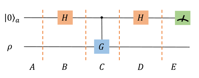
Figure 1: Illustrative diagram of the Hadamard Test circuit. The diagram features two distinct paths, which have been divided into five segments for ease of computation. The first path encompasses two $H$ gates and a single measurement gate, while the second path incorporates a $controlled-G$ gate.

In the region denoted as $\mathrm{A}$, the quantum state of the circuit at this point is given by:

$$|0\rangle\langle 0|\otimes\rho.$$ (1)

In the $\mathrm{B}$ region, after applying the Hadamard gate, the state of the ancillary qubit is transformed as Eq.(2):

$$\mathrm{H}|0\rangle\langle 0|\mathrm{H}^{\dagger}=\frac{1}{2}(|0\rangle\langle 0|+|0\rangle\langle 1|+|1\rangle\langle 0|+|1\rangle\langle 1|).$$ (2)

The overall state of the circuit is given by:

$$\frac{1}{2}(|0\rangle\langle 0|+|0\rangle\langle 1|+|1\rangle\langle 0|+|1\rangle\langle 1|)\otimes\rho.$$ (3)

Then, the state undergoes the action of the controlled $\mathrm{G}$ gate $CG^{k}$ :

$$CG^{k}=|0\rangle\langle 0|\otimes I+|1\rangle\langle 1|\otimes G^{k}.$$ (4)

Thus, the state in the region $\mathrm{C}$ is:

$$\begin{split}&\frac{1}{2}(|0\rangle\langle 0|\otimes\rho)+\frac{1}{2}|0\rangle\langle 1|\otimes\rho(G^{k})^{\dagger})+\\ &\frac{1}{2}|1\rangle\langle 0|\otimes G^{k}\rho)+\frac{1}{2}|1\rangle\langle 1|G^{k}\rho(G^{k})^{\dagger}.\end{split}$$ (5)

Subsequently, the auxiliary qubit undergoes another $\mathrm{Hadamard}$ gate operation. Consequently, the state within the region $\mathrm{D}$ is then given by:

$$\begin{split}&\frac{1}{2}\left[(H|0\rangle\langle 0|H^{\dagger})\otimes\rho+(H|0\rangle\langle 1|H^{\dagger})\otimes\rho(G^{k})^{\dagger}\right.\\ &\left.+(H|1\rangle\langle 0|H^{\dagger})\otimes G^{k}\rho+(H|1\rangle\langle 1|H^{\dagger})\otimes G^{k}\rho(G^{k})^{\dagger}\right].\end{split}$$ (6)

Expanding each term results as:

$$\frac{1}{4}|0\rangle\langle 0|\otimes[\rho+\rho(G^{k})^{\dagger}+(G^{k})\rho+(G^{k})\rho(G^{k})^{\dagger}],$$ (7)

$$\frac{1}{4}|0\rangle\langle 1|\otimes[\rho-\rho(G^{k})^{\dagger}+(G^{k})\rho-(G^{k})\rho(G^{k})^{\dagger}],$$

$$\frac{1}{4}|1\rangle\langle 0|\otimes[\rho+\rho(G^{k})^{\dagger}-(G^{k})\rho-(G^{k})\rho(G^{k})^{\dagger}],$$

$$\frac{1}{4}|1\rangle\langle 1|\otimes[\rho-\rho(G^{k})^{\dagger}-(G^{k})\rho+(G^{k})\rho(G^{k})^{\dagger}].$$

The expression above can be denoted as follows:

$$\rho^{\prime}=|0\rangle\langle 0|\otimes a_{11}+|0\rangle\langle 1|\otimes a_{12}+|1\rangle\langle 0|\otimes a_{21}+|1\rangle\langle 1|\otimes a_{22}$$ (8)

Under the computational basis measurement in region $\mathrm{E}$, the measurement operators are defined as $M_{0}=|0\rangle\langle 0|\otimes I$ and $M_{1}=|1\rangle\langle 1|\otimes I$. The probability distribution over the outcomes of the measurement are :

$${P}(0) =\mathrm{Tr}\{M_{0}\rho^{\prime}M_{0}^{\dagger}\}=|a_{11}|^{2}$$ (9)

$$=\frac{1}{2}+\frac{1}{2}\mathrm{Tr}\{G^{k}\rho\},$$

$${P}(1) =\mathrm{Tr}\{M_{1}\rho^{\prime}M_{1}^{\dagger}\}=|a_{22}|^{2}$$ (10)

$$=\frac{1}{2}-\frac{1}{2}\mathrm{Tr}\{G^{k}\rho\}.$$

The expression for $\mathrm{Tr}\{G^{k}\rho\}$ can be derived, with the ultimate goal of estimating:

$$\mathrm{Tr}\{\rho^{m+1}\} =\mathrm{Tr}\{(\frac{1}{2}I-\frac{1}{2}G)^{m}\rho\}$$ (11)

$$=\frac{1}{2^{m}}\sum_{k=0}^{m}C_{m}^{k}(-1)^{k}\mathrm{Tr}\{G^{k}\rho\}.$$

Let: $p_{k}=\frac{1}{2^{m}}C_{m}^{k}$, $x_{k}=(-1)^{k}\mathrm{Tr}\{G^{k}\rho\}$. The above equation can be transformed into an expectation calculation:

$$\mathrm{Tr}\{\rho^{m+1}\}=\sum_{k=0}^{m}p_{k}x_{k}=E_{k}(x_{k}).$$ (12)

To estimate the expectation, we need to generate quantum circuits using a random sampling method. For each circuit, we sample $m$ times, with a $1/2$ probability of adding a $CG$ gate to the circuit and a $1/2$ probability of doing nothing. After generating multiple circuits, we take the average of the results.

II.2 Algorithm for calculating $\mathrm{Tr}\{\rho^{m+1}\}$.

The pseudocode below, referred to as Algorithm II.2, is for calculating $\mathrm{Tr}\{\rho^{m+1}\}$.

Input:$n$,$p_{i}$,$U_{i}$,$N$

Output:$\mathrm{Tr}\{\rho^{m+1}\}$

1:Set the initial state to $|0\rangle^{\otimes n+1}$.

2:Randomly select $U_{i}$ with probability $p_{i}$ to act on the target qubits.

3:Apply a Hadamard gate to the ancilla qubit.

4:Sample $m$ times, with a $1/2$ probability of adding a $CG$ gate to the circuit and a $1/2$ probability of doing nothing.

5:Apply another Hadamard gate to the ancilla qubit.

6:Perform a computational basis measurement on the auxiliary qubit circuit.

7:Repeat the above steps $N$ times and take the average.

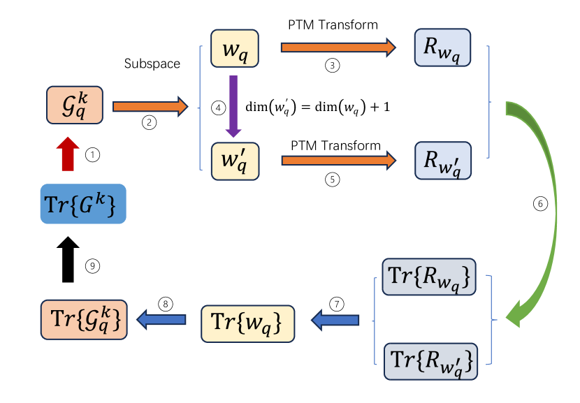
Figure 2: Process of calculating $\mathrm{Tr}\{G^{k}\}$ using Gate Set Tomography. Firstly, in Step 1, decompose $\mathrm{Tr}\{G^{k}\}$ into the calculation of each $\mathrm{Tr}\{\mathcal{G}_{q}^{k}\}$. Then, take its subspace $w_{q}$ (Step 2) and transform the matrix representation of the subspace into the corresponding Pauli Transfer Matrix, denoted as $R_{w_{q}}$. Simultaneously, in Step 4, expand the subspace $w_{q}$ by one dimension. Next, similarly, transform its matrix representation $w^{\prime}_{q}$ into its corresponding Pauli Transfer Matrix, denoted as $R_{w^{\prime}_{q}}$. Then, through Step 6, calculate their traces separately. By employing certain mathematical techniques in Step 7, we can use the obtained traces to calculate $\mathrm{Tr}\{w_{q}\}$, and subsequently obtain $\mathrm{Tr}\{\mathcal{G}_{q}^{k}\}$ (Step 8). Finally, in Step 9, we obtain $\mathrm{Tr}\{G^{k}\}$, which can be seen as the inverse process of Step 1.

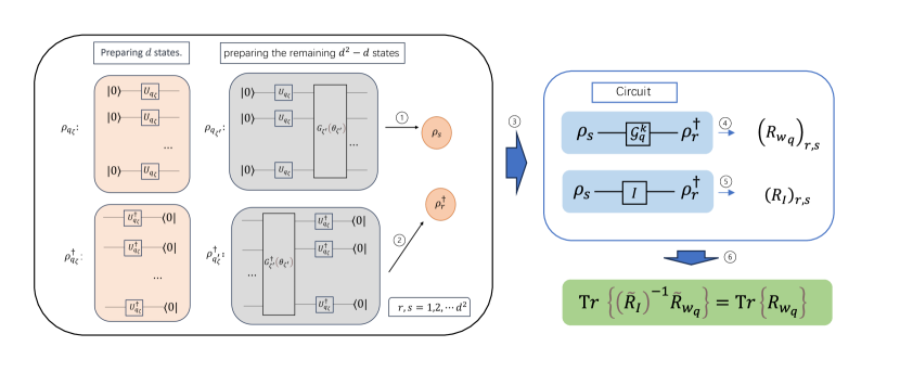
Figure 3: Schematic diagram of a sub-process for computing $\mathrm{Tr}\{R_{w_{q}}\}$ within the Tomography workflow. The diagram runs from left to right, with the first black box on the left representing the preparation of the initial state $(1)$ and the measurement state $(2)$. The blue box on the upper right depicts the placement of the prepared states into the circuit $(3)$, where the $\mathcal{G}_{q}^{k}$ gate and the identity gate are inserted. Steps $(4)$ and $(5)$ allow us to obtain the matrix elements of the PTMs corresponding to each of these gates. Finally, in step $(6)$, $\mathrm{Tr}\{R_{w_{q}}\}$ is indirectly obtained through a similarity transformation.

III Trace Estimation of Quantum Tomography

III.1 Theoretical Part of Quantum Tomography

Quantum tomography denotes a suite of techniques aiming to reconstruct an unknown quantum channel or state through experimental measurements. This process is pivotal for the comprehensive understanding and authentication of quantum apparatus greenbaum2015introduction; torlai2018neural; cramer2010efficient; mohseni2008quantum; altepeter2003ancilla. Nevertheless, the scalability of quantum tomography poses a challenge, as the indispensable measurements and computational resources experience exponential growth in tandem with qubit numbers. Note that although the resources required for tomography can be reduced by representing quantum states as MPS, in the worst case the resources required for tomography still increase exponentially with the number of bits cramer2010efficient; lanyon2017efficient. In the context of our current research problem, there is a silver lining: the subspace we are investigating maintains a dimension that remains unaffected by the number of qubits. This distinctive feature becomes particularly advantageous. In the subsequent section, we expound on our utilization of the GST method to extract the pertinent information from this designated subspace.

In comparison with the preceding context, the process of preparing random quantum states adheres to the same approach as the Hadamard Test method. This methodology necessitates the application of an assortment of stochastically selected gates $\{(U_{i})_{2^{n}\times 2^{n}},i=1,2,\ldots,\alpha\}$ onto the initial quantum state (typically $|0\rangle\langle 0|^{\otimes n}$), resulting in the emergence of a random quantum state. The primary objective revolves around the computation of $\mathrm{Tr}\{\rho^{m}\}$, which is achieved through the intermediary of $\mathrm{Tr}\{G^{m}\}$, where $G=I-2\rho$. We can express $\mathrm{Tr}\{\rho^{m}\}$ as

$$\mathrm{Tr}\{\rho^{m}\}=\frac{1}{2^{m}}\sum_{k=0}^{m}C_{m}^{k}(-1)^{k}\mathrm{Tr}\{G^{k}\}.$$ (13)

Similar to the approach employed in the HT-based algorithm, we can estimate this summation by leveraging the Monte Carlo method. This involves conducting multiple circuit samplings in accordance with their respective probabilities and subsequently calculating the average. Through this process, we can attain the sought-after value of $\mathrm{Tr}\{\rho^{m}\}$. The figure shown in Fig 2 presents our computation process through a simplified flowchart, starting from the decomposition of $\mathrm{Tr}\{G^{k}\}$, transitioning to the calculation of each individual $\mathcal{G}_{q}^{k}$, and then proceeding with a series of computations within their respective subspaces. Finally, the computed results $\mathrm{Tr}\{\mathcal{G}_{q}^{k}\}$ are weighted and summed to obtain the desired calculation $\mathrm{Tr}\{G^{k}\}$. We illustrate the sub-process of computing $\mathrm{Tr}\{R_{w_{q}}\}$ in Fig 3, which, together with Fig 2, forms the complete Tomography computation process.

III.1.1 Mathematical Treatment:

We start with the unitary quantum gate $G_{0}$:

$$(G_{0})_{2^{n}\times 2^{n}}=I_{2^{n}}-2|0\rangle\langle 0|^{\otimes n}=\begin{pmatrix}-1&0&\cdots&0\\ 0&1&\cdots&0\\ \vdots&\vdots&\ddots&\vdots\\ 0&0&\cdots&1\end{pmatrix}.$$ (14)

Through the application of random unitary gates $U_{i}$ to the initial gate $G_{0}$, a set of $\alpha$ distinct gates is generated. These gates are denoted as $G_{i}=U_{i}G_{0}U_{i}^{\dagger}$. The composite gate $G$ is then defined as the weighted summation of these transformed gates: $G=\sum_{i=1}^{\alpha}p_{i}G_{i}$.

An insightful observation can be made that in the presence of $k$ occurrences of $G$ gates within the circuit, the total count of possible arrangements aggregates to $\alpha^{k}$. These arrangements are uniquely labeled by the index $q=\{1,2,\ldots,\alpha^{k}\}$. As a result, this algorithm effectively dissects the trace $\mathrm{Tr}\{G^{k}\}$ of the higher-order powers of $G$ into computations encompassing $\alpha^{k}$ arrangements denoted as $\mathcal{G}^{k}_{q}$. The calculation process is thereby executed on higher-order random quantum states via the application of a Monte Carlo methodology.

The corresponding probability combination $\prod_{t=1}^{k}p_{q_{t}}$ is represented as $\mathcal{P}_{q}$. Therefore, $\mathrm{Tr}\{G^{k}\}$ can be expressed as:

$$\mathrm{Tr}\{{G}^{k}\}=\sum_{q=1}^{\alpha^{k}}\mathcal{P}_{q}\mathrm{Tr}\{\mathcal{G}_{q}^{k}\},$$ (15)

Where we use $\mathcal{G}^{k}_{q}$ to denote $\prod_{t=1}^{k}G_{q_{t}}$ for convenience.

III.1.2 The matrix representation of $\mathcal{G}_{q}^{k}$

For each of the $\alpha^{k}$ instances of $\mathcal{G}_{q}^{k}$, a specific $\mathcal{G}_{q}^{k}$ is chosen for computation where $q=1,2,\ldots,\alpha^{k}$. In this scenario, the calculation method is provided for arbitrary combinations, while the computation process remains similar for other combinations.

Upon choosing a specific combination $\mathcal{G}_{q}^{k}$, a set of $k$ corresponding $G_{q_{t}}$ gates is determined, thereby giving rise to $k$ specific $|\psi_{q_{t}}\rangle$ states, where $t=1,2,\ldots,k$.

For example, consider the cases:

$$q=1,\{\mathcal{G}_{1}^{k}:\underbrace{G_{1}G_{1}\cdots G_{1}G_{1}}_{k\ layers}\}.$$

$$q=2,\{\mathcal{G}_{2}^{k}:\underbrace{G_{1}G_{1}\cdots G_{1}G_{2}}_{k\ layers}\}.$$

$$\quad\vdots$$

$$q=\alpha^{k},\{\mathcal{G}_{\alpha^{k}}^{k}:\underbrace{G_{\alpha}G_{\alpha}\cdots G_{\alpha}G_{\alpha}}_{k\ layers}\}.$$

Therefore, under the matrix background denoted as $\mathcal{G}_{q}^{k}$, the subspace dimension $d$ is not constant. Hence, the determination of the subspace dimension relies entirely on the count of unique gate types present in the given order $q$. Let us define $d$ as the dimension of the nontrivial subspace corresponding to the simplified merge of $\mathcal{G}_{q}^{k}:=\prod_{t=1}^{k}G_{q_{t}}$, while representing the random gate sets used to prepare $G_{q_{t}}$ as $U_{q_{t}}$: $G_{q_{t}}=U_{q_{t}}G_{0}U_{q_{t}}^{\dagger}$. Quantum states prepared by different random gates are represented as: ${|\psi_{q_{\zeta}}\rangle,\zeta=1,2,\ldots,d}$.

In order to ensure completeness, a set of state vectors $\{|\phi_{\eta}\rangle,\eta=1,2,\cdots,2^{n}-d\}$ is introduced, which are orthogonal to all the state vectors $|\psi_{q_{\zeta}}\rangle$.

The rationale behind this is as follows:

Due to the condition $\langle\psi_{q_{\zeta}}|\phi_{\eta}\rangle=0$, it can be inferred that:

$$\mathcal{G}_{q}^{k}(|\phi_{\eta}\rangle)=\left[\prod_{\zeta=1}^{d}(I-2(|\psi_{q_{\zeta}}\rangle\langle\psi_{q_{\zeta}}|)\right]|\phi_{\eta}\rangle=|\phi_{\eta}\rangle.$$

It is evident that $\{{|\phi_{\eta}\rangle},\eta=1,2,\dots,2^{n}-d\}$ forms a set of eigenstates of $\mathcal{G}_{q}^{k}$ with eigenvalue $1$. In the representation with $2^{n}$ state vectors:

$$\left\{\underbrace{|\psi_{q_{1}}\rangle,|\psi_{q_{2}}\rangle,\ldots,|\psi_{q_{d}}\rangle}_{d\ \text{terms}},\underbrace{|\phi_{1}\rangle,|\phi_{2}\rangle,\ldots,|\phi_{\eta}\rangle}_{(2^{n}-d)\ \text{terms}}\right\}.$$ (16)

as the basis in the $V_{q}$ space, the matrix $\mathcal{G}_{q}^{k}$ can be expressed as:

$$\left(\begin{array}[]{ccccccc}w_{11}&w_{12}&\ldots&w_{1d}&0&0&\ldots\\ w_{21}&w_{22}&\ldots&w_{2d}&0&0&\ldots\\ \ldots&\ldots&\ldots&\ldots&0&0&\ldots\\ w_{d1}&w_{d2}&\ldots&w_{dd}&0&0&\ldots\\ 0&0&0&0&1&0&\ldots\\ 0&0&0&0&0&\ldots&\ldots\\ \ldots&\ldots&\ldots&\ldots&\ldots&\ldots&1\\ \end{array}\right)$$ (17)

The top-left $d\times d$ matrix $w_{q}$ can be considered as composed of the eigenvalues of the $d$-dimensional invariant subspace $V_{q1}$ spanned by $d$ states $|\psi_{q_{\zeta}}\rangle$ in the basis. The remaining part of $\mathcal{G}_{q}^{k}$ is composed of the eigenvectors in the complement space with basis ${|\phi_{\eta}\rangle}$, corresponding to $(2^{n}-d)$ eigenvalues. These eigenvalues form an $(2^{n}-d)\times(2^{n}-d)$ identity matrix $I_{(2^{n}-d)\times(2^{n}-d)}$. Therefore, $w_{q}$ is actually the matrix representation of $\mathcal{G}_{q}^{k}$ in the $d$-dimensional invariant subspace $V_{q1}$. Through this expression, the calculation of $\mathrm{Tr}\{\mathcal{G}_{q}^{k}\}$ can be performed:

$$\mathrm{Tr}\{\mathcal{G}_{q}^{k}\} =\mathrm{Tr}\{w_{q})+\mathrm{Tr}\{I_{2^{n}-d}\}$$ (18)

$$=\mathrm{Tr}\{w_{q}\}+2^{n}-d.$$

III.1.3 The PTM representation of $w_{q}$

After characterizing $\mathcal{G}_{q}^{k}$, we need to obtain the solution for $\mathrm{Tr}\{w_{q}\}$. However, the matrix $w_{q}$ is unknown. $w_{q}$ as a mapping, finding the solution for $w_{q}$ requires the use of the Pauli Transfer Matrix(PTM). We denote the PTM corresponding to $w_{q}$ as $R_{w_{q}}$.

Based on the previous discussion, an important relationship can be used:

$$R_{w_{q}}|\rho_{s}\rangle\rangle =|w_{q}(\rho_{s})\rangle\rangle=|w_{q}\rho_{s}w_{q}^{\dagger}\rangle\rangle$$

$$r,s\in\{1,2,\ldots,d^{2}\}.$$

For simplicity, the subscript $q$ indicating that $\rho$ belongs to the ordering $\mathcal{G}_{q}^{k}$ will be omitted below.

Although $R_{w_{q}}$ is an $(d^{2}\times d^{2})$ matrix, the vector $|\rho_{s}\rangle\rangle$ has dimensions of $(2^{n})^{2}\times 1$. Since $|\rho_{s}\rangle\rangle$ only has non-zero elements in the $d^{2}$-dimensional subspace, the remaining part of the vector is trivial, consisting of all zeros except for this subspace.

By left-multiplying the above equation by $\langle\langle\rho_{r}|$, the matrix elements of the $PTM$ matrix $(R_{w_{q}})_{d^{2}\times d^{2}}$ are given as follows:

$$\langle\langle\rho_{r}|R_{w_{q}}|\rho_{s}\rangle\rangle=\langle\langle\rho_{r}|w_{q}\rho_{s}w_{q}^{\dagger}\rangle\rangle.$$ (19)

To calculate the matrix elements $(R_{w_{q}})_{rs}$ of $R_{w_{q}}$ using this method, $d^{2}$ quantum states in the Hilbert-Schmidt space are required, represented by vectors $|\rho_{r}\rangle\rangle$. The proof of the completeness of these states can be found in Appendix LABEL:Appendix_A:_Completeness_Proof.

We need to calculate the trace of PTM. Although we can obtain each matrix element of the PTM sequentially through the circuit, we cannot directly compute its trace because the basis vectors in the subspace we generate are not orthogonal. There are two feasible approaches:Schmidt decomposition to orthogonalize its basis vectors, and then directly calculate the trace by summing the main diagonal elements;Calculate its trace indirectly through a matrix similarity transformation.This paper adopts the GST (Gate Set Tomography) method, which is the latter approach of indirectly calculating the trace of PTM through similarity transformations.

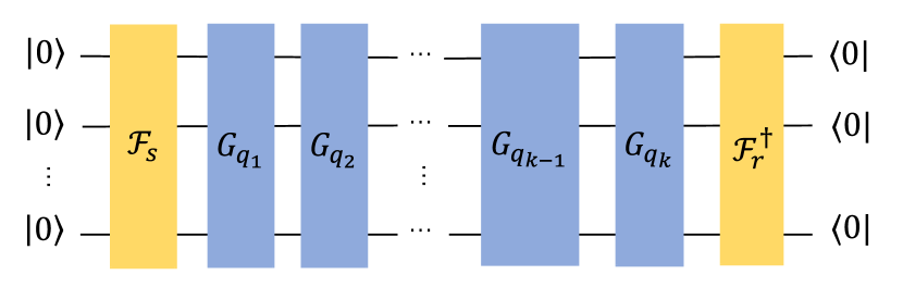
Figure 4: This is a quantum circuit with n-Qubits used to compute Tr{$\rho_{r}^{\dagger}\mathcal{G}_{q}^{k}\rho_{s}\mathcal{G}_{q}^{k}$}. First, we add the prepared state $\rho_{r}^{\dagger}$ to the circuit. Next, we apply the operator $\mathcal{G}_{q}^{k}$. Then, we add $\rho_{s}$ to the circuit.

III.1.4 GST

In Quantum Process Tomography (QPT), the information required to reconstruct each gate $R_{w_{q}}$ is contained in the measurements of $\langle\langle\rho_{r}|R_{w_{q}}|\rho_{s}\rangle\rangle$, and $R_{w_{q}}$ is the PTM of $w_{q}$ in the Hilbert-Schmidt space. QPT assumes that the initial state and final measurements are known. In practice, these states and measurements must be prepared using quantum gates, and these gates $\{F_{r},F_{s}^{\prime}\}$ themselves may have imperfections greenbaum2015introduction:

$$\langle\langle\rho_{r}| =\langle\langle 0|F_{r},$$

$$|\rho_{s}\rangle\rangle =F_{s}^{\prime}|0\rangle\rangle.$$

Indeed, the initial states and final measurements that were prepared using gates are not directly known and can introduce errors in the estimation process. GST aims to characterize the fully unknown set of gates and statesblume2013robust.

$$\mathcal{R}=\{|\rho\rangle\rangle,\langle\langle E|,R_{w_{1}},\ldots,R_{w_{q}},\ldots\},q=1,2,\ldots,\alpha^{k}.$$ (20)

GST has similar requirements to QPT: the ability to measure the set of gates $\mathcal{R}=\{|\rho\rangle\rangle,\langle\langle E|,R_{w_{1}},\ldots,R_{w_{\alpha^{k}}}\}$ in the form of expectation values:

$$p=\mathrm{Tr}\{\rho_{r}^{\dagger}w_{q}(\rho_{s})\}=\langle\langle\rho_{r}|R_{w_{q}}|\rho_{s}\rangle\rangle=\mathrm{Tr}\{\rho_{r}^{\dagger}w_{q}\rho_{s}w_{q}^{\dagger}\}.$$

To simplify the expression, we use ${{F_{r},F_{s}^{\prime}}}$, where $(r,s=1,2,\ldots,d^{2})$, to denote the quantum gates used for preparing quantum states and measurements (as shown in Fig 4), which are ${G_{q_{r}}(\theta_{r})U_{q_{r}}}$ and ${U_{q_{s}}^{\dagger}G_{q_{s}}^{\dagger}(\theta_{s})}$, respectively. The density matrices of these prepared quantum states are linearly independent. Please refer to Appendix LABEL:Appendix_A:_Completeness_Proof for details. By constructing a quantum circuit, it is possible to compute the $d^{2}$ matrix elements of the PTM matrix $R_{w_{q}}$. We define $(R_{w_{q}})_{rs}$ as follows:

$$(R_{w_{q}})_{rs}=\langle\langle\rho_{r}|R_{w_{q}}|\rho_{s}\rangle\rangle=\langle\langle 0|F_{r}R_{w_{q}}F_{s}|0\rangle\rangle.$$ (21)

Inserting the completeness state into it yields:

$$p_{rs} =(R_{w_{q}})_{rs}=\langle\langle\rho_{r}|R_{w_{q}}|\rho_{s}\rangle\rangle$$

$$=\langle\langle 0|F_{r}R_{w_{q}}F_{s}|0\rangle\rangle$$

$$=\sum_{a,b}\langle\langle 0|F_{r}|a\rangle\rangle\langle\langle a|R_{w_{q}}|b\rangle\rangle\langle\langle b|F_{s}|0\rangle\rangle$$

$$=\sum_{a,b}A_{ra}(R_{w_{q}})B_{bs}.$$

It can be easily verified that:

$$p_{rs} =(AR_{w_{q}}B)_{rs},$$ (22)

$$A =\sum_{r}|r\rangle\rangle\langle\langle 0|F_{r},$$

$$B =\sum_{s}F_{s}|0\rangle\rangle\langle\langle s|.$$

Let $\tilde{R}_{w_{q}}=AR_{w_{q}}B$, the identity matrix $I$ also serves as a mapping, and its PTM has the following properties:

$$R_{I}|\rho_{s}\rangle\rangle=|I(\rho_{s})\rangle\rangle=|I\rho_{s}I^{\dagger}\rangle\rangle=|\rho_{s}\rangle\rangle.$$

It can be observed that the action of $R_{I}$ is similar to the identity matrix and its matrix elements can be expressed as follows:

$$(R_{I})_{rs} =\langle\langle\rho_{r}|R_{I}|\rho_{s}\rangle\rangle=\mathrm{Tr}\{\rho_{r}^{\dagger}I\rho_{s}I^{\dagger}\}=\mathrm{Tr}\{\rho_{r}^{\dagger}\rho_{s}\}.$$

Denoting $g_{rs}=(R_{I})_{rs}=\langle\langle\rho_{r}|\rho_{s}\rangle\rangle=\langle\langle 0|F_{r}F_{s}|0\rangle\rangle$, we can insert the completeness state and obtain:

$$g_{rs}=\sum_{a,b}\langle\langle 0|F_{r}|a\rangle\rangle\langle\langle a|b\rangle\rangle\langle\langle b|F_{s}|0\rangle\rangle=(AB)_{rs}.$$ (23)

For a given combination $\mathcal{G}^{k}_{q}$, let $\tilde{R}_{I_{q}}=AB$, where $A$ and $B$ are matrices. The experimental measurement value $p_{rs}$ corresponds to the $rs$ component of the matrix $A(R_{w_{q}})B$, while $g_{rs}$ corresponds to the $rs$ component of the matrix $(AB)$. The quantum channel we reconstruct will differ from the real quantum channel by a similarity transformation:

$$(\tilde{R}_{I})^{-1}\tilde{R}_{w_{q}}=B^{-1}A^{-1}AR_{w_{q}}B=B^{-1}R_{w_{q}}B.$$

Therefore, we can estimate the trace of $R_{w_{q}}$:

$$\mathrm{Tr}\{(\tilde{R}_{I})^{-1}\tilde{R}_{w_{q}}\}=\mathrm{Tr}\{B^{-1}R_{w_{q}}B\}=\mathrm{Tr}\{R_{w_{q}}\}.$$ (24)

Based on the calculations mentioned earlier, the value of $\mathrm{Tr}\{R_{w_{q}}\}=|\mathrm{Tr}\{w_{q}\}|^{2}$ can be determined. However, this is not the final result for $\mathrm{Tr}\{w_{q}\}$.

Note: In order to avoid ill-conditioned matrices $R_{I_{q}}$, it is necessary to perform subspace selection. For detailed analysis, please refer to Section LABEL:Eigenvalue_Truncation.

III.1.5 Mathematical Processing of Results

To calculate $\mathrm{Tr}\{w_{q}\}$, an operation involving taking the square root is required: $|\mathrm{Tr}\{w_{q}\}|^{2}=\mathrm{Tr}\{R_{w_{q}}\}$. In general, $\mathrm{Tr}\{w_{q}\}$ can be decomposed into real and imaginary parts:

$$\mathrm{Tr}\{w_{q}\}=\mathbf{\text{Re}}[\mathrm{Tr}\{w_{q}\}]+i\cdot\mathbf{\text{Im}}[\mathrm{Tr}\{w_{q}\}].$$

then

$$\mathrm{Tr}\{R_{w_{q}}\}=(\mathbf{\text{Re}}[\mathrm{Tr}\{w_{q}\}])^{2}+(\mathbf{\text{Im}}[\mathrm{Tr}\{w_{q}\}])^{2}.$$

In fact, only the real part needs to be estimated because the sum of all the imaginary parts of $\mathrm{Tr}\{w_{q}\}$ vanishes after summation.

$$\sum_{q=1}^{\alpha^{k}}\mathrm{Tr}\{w_{q}\}=\sum_{q=1}^{\alpha^{k}}\mathbf{\text{Re}}[\mathrm{Tr}\{w_{q}\}].$$ (25)

Next, we show how to estimate the real part of $\mathrm{Tr}\{w_{q}\}$. Consider $(w^{\prime}_{q})_{d+1}=(w_{q})_{d}\oplus 1$, where $w_{q}^{\prime}$ is the representation of $\mathcal{G}_{q}^{k}$ on the subspace $V_{q}^{\prime}:span\{|\psi_{q_{1}}\rangle,|\psi_{q_{2}}\rangle,\cdot\cdot,|\psi_{q_{d}}\rangle;|\phi\rangle\}$.

$$w_{q}^{\prime}=\begin{pmatrix}w_{q}&0\\ 0&1\\ \end{pmatrix},$$

where $|\phi\rangle\notin V_{q}$ and $|\phi\rangle$ can be prepared through a variational quantum circuit. It can be seen that $V_{q}^{\prime}$ is also a noninvariant subspace of $\mathcal{G}_{q}^{k}$. It’s obvious that

$$\mathrm{Tr}\{w_{q}^{\prime}\}=\mathrm{Tr}\{w_{q}\}+1,$$ (26)

and:

$$\mathrm{Tr}\{R_{w^{\prime}_{q}}\} =|\mathrm{Tr}\{w^{\prime}_{q}\}|^{2}=|\mathrm{Tr}\{w_{q}\}+1|^{2}$$ (27)

$$=\left|\text{Re}[\mathrm{Tr}\{w_{q}\}]+i\cdot\text{Im}[\mathrm{Tr}\{w_{q}\}]+1\right|^{2}$$

$$=(\text{Re}[\mathrm{Tr}\{w_{q}\}])^{2}+2(\text{Re}[\mathrm{Tr}\{w_{q}\}])$$

$$+(\text{Im}[\mathrm{Tr}\{w_{q}\}])^{2}+1.$$

Recall the relation

$$\mathrm{Tr}\{R_{w}\} =|\mathrm{Tr}\{w_{q}\}|^{2}$$

$$=(\text{Re}[\mathrm{Tr}\{w_{q}\}])^{2}+(\text{Im}[\mathrm{Tr}\{w_{q}\}])^{2},$$

we can find that

$$\text{Re}[\mathrm{Tr}\{w_{q}\}]=\frac{1}{2}[\mathrm{Tr}\{R_{w^{\prime}_{q}}\}-\mathrm{Tr}\{R_{w_{q}}\}-1].$$ (28)

The procedure to calculate $\mathrm{Tr}\{R_{w^{\prime}_{q}}\}$ follows a similar algorithm as for computing $\mathrm{Tr}\{R_{w_{q}}\}$, with the distinction that in this case, $(d+1)^{2}$ quantum states are required.

III.2 Algorithm Process of Tomography

The following is the procedure for calculating $\mathrm{Tr}\{\rho^{m}\}$ for the quantum state $\rho=\sum_{i=1}^{\alpha}p_{i}U_{i}|0\rangle\langle 0|U_{i}^{\dagger}$.Algorithm III.2 serves as the main program for GST, while Algorithm III.2 functions as a subroutine called multiple times within GST, responsible for iteratively computing $\mathrm{Tr}\{\mathcal{G}_{q}^{k}\}$.

Input:$N$,$m$,$p_{i}$,$U_{i}$,$\alpha$,$n$
Output:$\mathrm{Tr}\{\rho^{m}\}$

1:for $\text{iteration}=1$ to $N$ do

2:     Set the initial state as $|0\rangle^{\otimes n}$.

3:     Initialise $d\leftarrow 0$

4:     Initialise the subspace $V_{q}\leftarrow[~{}]$.

5:     // Dimension of the subspace is determined.

6:     for $i=1$ to $m$ do

7:         Randomly choose Gate with probability $1/2$ (for $G$ ) or $1/2$ (for $I$ ).

8:         If it is a $G$ gate, choose $G_{i}$ with probability $p_{i}$.

9:     end for

10:     // Select $\mathcal{G}_{q}^{k}$ with probability $\mathcal{P}_{q}$

11:     for $i=1$ to $k$ do

12:         // Here $k$ is the number of $G$ in $G_{q}^{k}$.

13:         Apply gate $U[i]$ to prepare quantum state $|\psi_{i}\rangle=U[i]|0\rangle^{\otimes n}$. $U[i]$ is the unitary corresponding to $i$th $G$ gate, $G[i]=U[i]G_{0}U[i]^{\dagger}$.

14:         Compute the Gram matrix $g_{i}$ in the subspace $V\oplus|\psi_{i}\rangle$.

15:         Compare eigenvalues of Gram matrix $\epsilon_{g}$ of $g_{i}$ with threshold $\epsilon$.

16:         // Perform linear correlation analysis on $|\psi_{i}\rangle$ states.

17:         if $\epsilon_{g}\geq\epsilon$ then

18:              Update the dimension $d\leftarrow d+1$.

19:              Update the subspace $V_{q}\leftarrow V_{q}\oplus|\psi_{i}\rangle$.

20:         end if

21:     end for

22:     $t_{1}\leftarrow$ Subroutine($\mathcal{G}_{q}^{k}$, $d$, $V_{q}$)

23:     $t_{2}\leftarrow$ Subroutine($\mathcal{G}_{q}^{k}$, $d+1$, $V_{q}\oplus|\phi\rangle$)

24:     $\mathrm{Tr}\{\mathcal{G}_{q}^{k}\}\leftarrow 2^{n}-d+(t_{1}-t_{2}-1)/2$.

25:     // Invoke the subroutine to calculate $\mathrm{Tr}\{\mathcal{G}_{q}^{k}\}$.

26:end for

27:Calculate $\mathrm{Tr}\{\rho^{m}\}=\mathrm{Tr}\left\{\left(\frac{1}{2}I-\frac{1}{2}G\right)^{m}\right\}=\sum_{k=0}^{m}p_{k}x_{k}$

28://$p_{k}=\left(\frac{1}{2}\right)^{m}C_{m}^{k}$ and $x_{k}=(-1)^{k}\mathrm{Tr}\{G^{k}\}$

Input:$\mathcal{G}_{q}^{k}$, $d$, $V$
Output:$\mathrm{Tr}\{R_{w_{q}}\}$

1:for $\zeta=1$ to $d$ do

2:     $\rho_{q_{\zeta}}=\left|\psi_{q_{\zeta}}\right\rangle\langle\psi_{q_{\zeta}}|=U_{q_{\zeta}}|0\rangle\langle 0|U_{q_{\zeta}}^{\dagger}$

3:end for

4:for $\zeta^{\prime}=1$ to $d$ do

5:     if $\zeta\neq\zeta^{\prime}$ then

6:         $\rho_{q_{\zeta^{\prime}}}=\left|\psi_{q_{\zeta^{\prime}}}\right\rangle\langle\psi_{q_{\zeta^{\prime}}}|$

7:         $\quad\quad=G_{\zeta^{\prime}}(\theta_{\zeta^{\prime}})U_{q_{\zeta}}|0\rangle\langle 0|U_{q_{\zeta}}^{\dagger}G_{\zeta^{\prime}}^{\dagger}(\theta_{\zeta^{\prime}})$

8:         //Prepare $(d^{2}-d)$ additional quantum states

9:     else

10:         Break // Exit the loop

11:     end if

12:end for

13:for $r=1$ to $d^{2}$  do

14:     for $s=1$ to $d^{2}$  do

15: