Data-Efficient Online Learning of Ball Placement in Robot Table Tennis

Abstract

We present an implementation of an online optimization algorithm for hitting a predefined target when returning ping-pong balls with a table tennis robot. The online algorithm optimizes over so-called interception policies, which define the manner in which the robot arm intercepts the ball. In our case, these are composed of the state of the robot arm (position and velocity) at interception time. Gradient information is provided to the optimization algorithm via the mapping from the interception policy to the landing point of the ball on the table, which is approximated with a black-box and a grey-box approach. Our algorithm is applied to a robotic arm with four degrees of freedom that is driven by pneumatic artificial muscles. As a result, the robot arm is able to return the ball onto any predefined target on the table after about $2$-$5$ iterations. We highlight the robustness of our approach by showing rapid convergence with both the black-box and the grey-box gradients. In addition, the small number of iterations required to reach close proximity to the target also underlines the sample efficiency. A demonstration video can be found here: https://youtu.be/VC3KJoCss0k.

I Introduction

I-A Background

Reinforcement learning (RL) has proven to be a powerful and general framework that has many applications in robotics [1, 2, 3, 4, 5] and beyond [6]. However, modern RL approaches rely on deep neural networks [7] and often require a large number of interactions with the environment until a reasonable policy is found. The search for a good policy is therefore often supported with numerical simulations which can be time-consuming and computationally expensive.

Another downside is that the performance of RL algorithms is often sensitive to hyperparameter tuning, which requires extensive supervision by engineers, and limits their online applicability. Nevertheless, online adaptation is important for many real-world applications, where the environment or the robot dynamics may (gradually) change [8].

In the following article, we propose an online optimization algorithm that mitigates some of these disadvantages. The algorithm uses gradient descent and allows for the incorporation of prior knowledge. We will evaluate our framework on a challenging robotic control task with a four-degrees-of-freedom robot arm driven by pneumatic artificial muscles (PAMs), see [9]. Our task is to enable the arm to return a ping-pong ball that is played to the robot back to any predefined target on the table. Our algorithm will iteratively update and learn the interception policy, where we take advantage of an already existing low-level controller that drives the robot arm, see [10]. We demonstrate that due to the inclusion of prior knowledge, our online optimization framework can be implemented in a data-efficient and robust manner.

I-B Related Work

Most of the recent and competitive table tennis robots use an adaptation of RL for their control. The authors of [11] combine an RL algorithm that is trained to adjust the robot’s joint trajectory with a regression model that predicts the ball’s trajectory and the robot’s joint trajectories. A combination of RL and imitation learning has been used by [12] and [13] and has shown strong results in terms of interception rates and landing point control, whereby [12] explicitly evaluates performance for different target locations on the table. To facilitate and accelerate the learning process, [14] developed a hybrid RL approach that simultaneously learns from a simulation and from executing a policy on the real-world system. The method is evaluated on a soft robot actuated by PAMs, which allows for safe exploration and thus removes the need for sophisticated policy initialization. All of these proposed methods use a high-dimensional action space that is searched through extensive trial and error, typically requiring thousands of iterations.

Online optimization, which can be seen as an instance of online learning, was popularized by [15] and has mostly been used in theoretical settings to derive sample-complexity bounds, convergence guarantees, and convergence rates for learning algorithms. What makes the formulation of online optimization interesting is that it allows for unknown and even adversarial cost functions. This is in line with our setup, where the incoming ball trajectories are different from execution to execution and the system dynamics are assumed to be unknown and potentially slowly time-varying.

The soft robotics actuation principle of PAMs has seen application in a broad range of fields. Examples include exoskeletons for assistance and rehabilitation [16, 17, 18, 19, 20], legged locomotion [21, 22, 23, 24] and various aerospace applications [25]. A collection of different designs and additional application examples can be found in [26, 27]. Many first-principle models of PAMs have been built in order to facilitate their control, and a detailed summary of such modeling approaches is found in [27]. Other control approaches that avoid utilizing sophisticated physical models include iterative learning control [10, 28] and RL [14].

I-C Contribution

The main contribution of our work is to propose a robust and data-efficient online optimization algorithm for solving learning tasks that arise in robotic systems. This contrasts traditional applications of online optimization algorithms, which mainly consist of machine learning applications such as recommendation systems, packet routing, or spam filtering [29]. More precisely, we apply our framework to a four-degrees-of-freedom robot arm that is driven by PAMs and is illustrated in Figure 1. The algorithm takes advantage of an existing low-level controller and is able to return balls to predefined targets with an accuracy of about $25\text{\,}\mathrm{cm}$. An important aspect of our framework is to build a mapping that connects the interception policy, which is defined as the state of the robot arm at interception time, to the Euclidean distance between the target and the landing point of the ball. The distance between the target and the landing point defines the loss in the online optimization and is measured by a vision system [30]. At each iteration, i.e., after each returned ball, the interception policy will be updated online by a gradient descent method, where the gradients are approximated with either a black-box or a grey-box approach.

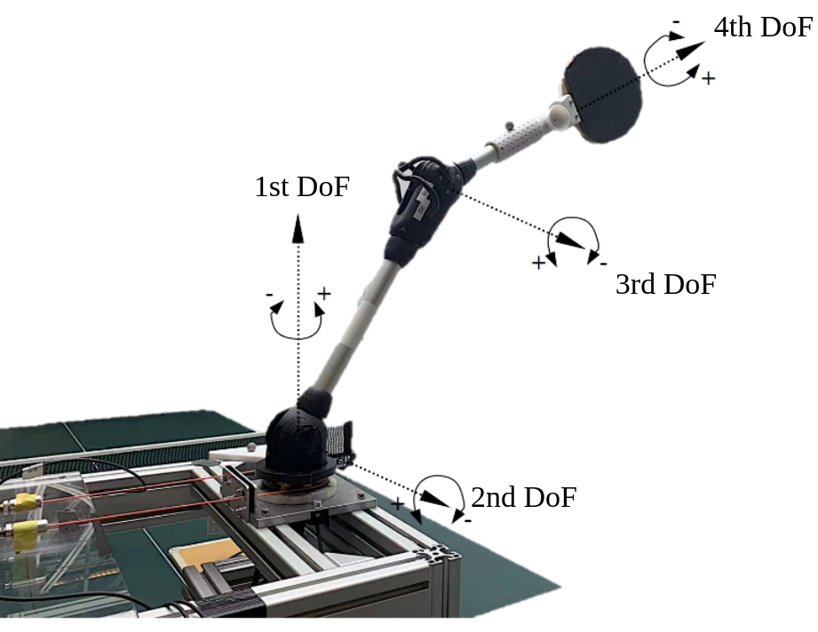
Figure 1: The figure shows the structure of the robot arm with its four rotational degrees of freedom (DoFs). Each joint is actuated by a pair of PAMs.

We note that the lack of gradient information due to the unknown underlying system dynamics is a key bottleneck, not only when applying online optimization algorithms to robotic systems, but also for RL in general. The traditional approach of using (stochastic) finite differences is often biased and has a high variance, which considerably slow down the optimization. Therefore, an important contribution of our work is to propose both a grey-box and a deep learning approach that approximate the mapping from the interception policy to the loss. We compare the results when employing either of the two mappings and find that in both cases the distance error converges toward zero (on average) at similar rates and with a similar variance.

Compared to existing RL algorithms for robotic systems such as Q-learning or actor-critic methods, our framework is very data efficient. In our extensive experiments that include different initial policies and different targets, our algorithm required only about $2$-$5$ iterations to hit a target with an error below $25\text{\,}\mathrm{cm}$. The algorithm is therefore directly applied to the real-world robotic system and does not require a simulator (although a simulator could be used to warm-start the online optimization, which would further reduce the number of iterations needed).

I-D Structure

This article is structured as follows: In Section II, we formulate the task of finding interception policies as an online optimization problem and describe the gradient descent algorithm that we use subsequently. In Section III, we describe two fundamentally different approaches for predicting the landing points (either grey-box or black-box), which will provide important gradient information to the optimization algorithm. The performance of both approaches will be evaluated in real-world experiments as described in Section IV. The article concludes with a summary in Section V.

II ONLINE OPTIMIZATION

II-A Problem Formulation

In our work, the robot arm learns to hit and return a ball shot from a launcher (presented in [31]) onto a predefined target $r_{\text{target}}\in\mathbb{R}^{2}$ on the table. We ensure that the $z$-coordinate of the global coordinate system stands orthogonal to the table, and unless otherwise specified, all the following calculations take place in the global coordinate system. The target is then within the $x$-$y$ plane at table height, that is, $r_{\text{target}}=\left(x_{\text{target}},y_{\text{target}}\right)^{\text{T}}$. Our approach can easily be extended to aim at a three-dimensional target in space.

In the following, $\theta_{j}$ and $\dot{\theta}_{j}$ denote the angle and angular velocity of degree of freedom $j\in\{1,2,3,4\}$. The landing point $r_{\text{landing}}\in\mathbb{R}^{2}$ after the ball is returned, also within the $x$-$y$ plane at the table height, is dependent on the interception policy $\phi\in\mathcal{K}\subseteq\mathbb{R}^{2}$, where $\mathcal{K}$ denotes the feasible set as described below. As illustrated in Figure 2, for a given ball trajectory the angle $\theta_{1}$ uniquely determines the interception time point, $t_{\text{ic}}$, as well as the angles $\theta_{2}$ and $\theta_{3}$ of the remaining degrees of freedom at time $t_{\text{ic}}$. At the interception time point, we fix the velocity $\dot{\theta}_{1}=$ $6\text{\,}\mathrm{rad}\text{\,}{\mathrm{s}}^{-1}$ and set the velocities $\dot{\theta}_{2}$, $\dot{\theta}_{3}$, and $\dot{\theta}_{4}$ to zero (this amounts to a straight return that does not induce extra spin). The algorithm works in the same way when $\dot{\theta}_{1}$, $\dot{\theta}_{2}$, or $\dot{\theta}_{3}$ are set to different values. Our interception policy therefore controls the interception time point and the angle of the return with $\theta_{1}$ and the distance of the return with $\theta_{4}$. We also conducted experiments where both $\theta_{4}$ and $\dot{\theta}_{1}$ were used to control the distance, but found that $\theta_{4}$ was the dominant factor, which led us to the choice

$$\phi=\left(\theta_{1}(t_{\text{ic}}),\theta_{4}(t_{\text{ic}})\right)^{\text{T}}.$$

The feasible set $\mathcal{K}$ is introduced to ensure that the interception policy does not exceed the physical limits of the robot arm and is chosen as $\mathcal{K}=\{\phi\in\mathbb{R}^{2}|-\frac{\pi}{2}\leq\theta_{1}(t_{\text{ic}})\leq\frac{\pi}{2},-\frac{\pi}{4}\leq\theta_{4}(t_{\text{ic}})\leq\frac{\pi}{4}\}$. The set is convex and thanks to the high compliance and power-to-weight ratio of the PAMs [9], it is large enough to cover the entire range of interception policies needed in practice.

(a) Top-down view

(b) 3D view

Figure 2: The figure shows a sketch of the robot arm. Subigure (a) illustrates how $\theta_{1}$ defines the interception point and subfigure (b) shows how this subsequently fixes $\theta_{2}$ and $\theta_{3}$ as well.

In the following, we assume that $r_{\text{landing}}$ can be divided into a deterministic part, $\tilde{r}_{\text{landing}}$, and an additive disturbance as follows:

$$r_{\text{landing}}\left(\phi,n\right)=\tilde{r}_{\text{landing}}\left(\phi\right)+n,$$

where the disturbance is non-repetitive and captures the fluctuation of the different incoming ball trajectories and the process noise of the robot arm. We note that according to the online learning/online optimization framework, [29], the disturbance is not necessarily required to be stochastic and zero mean for our framework to perform well.

For any fixed target, the learning task will be formulated as the following online optimization problem:

$$\begin{split}&\sum_{i=1}^{N}L^{i}(\phi^{i})\rightarrow\text{min},\\ &\text{where }\phi^{i}\in\mathcal{K},L^{i}(\phi^{i})=\frac{1}{2}|r_{\text{landing}}(\phi^{i},n^{i})-r_{\text{target}}|^{2},\\ &\text{for all }i=1,\dots,N,\end{split}$$ (1)

where $N$ denotes the number of iterations (not necessarily fixed). We denote by $|\cdot|$ the Euclidean distance and by the superscript $\left(\cdot\right)^{i}$ the iteration number. The non-repetitive disturbance $n^{i}$ leads to an iteration-dependent loss function with the interception policy as its only argument. We note that at the iteration $i$ the optimization algorithm has only access to the data from previous iterations $l=i-1,\dots,1$ while the disturbance $n^{i}$ is unknown.

II-B Online Gradient Descent

We optimize (LABEL:eq:loss) by applying online gradient descent, where according to the chain rule, the gradient of the loss function at each iteration is calculated as follows:

$$\nabla L^{i}(\phi^{i})=\underbrace{\left(\frac{\partial\tilde{r}_{\mathrm{landing}}\left(\phi^{i}\right)}{\partial\phi}\right)^{\mathrm{T}}}_{\text{Part 1}}\underbrace{(r_{\mathrm{landing}}\left(\phi^{i},n^{i}\right)-r_{\mathrm{target}})}_{\text{Part 2}},$$

with $i=1,\dots,N$. We note that the value of Part $2$ can be easily obtained because $r_{\text{target}}$ is predefined and fixed, and $r_{\text{landing}}\left(\phi^{i},n^{i}\right)$ at the $i$-th iteration is observed by the vision system. In contrast, the value of Part $1$ is more difficult to determine, since the mapping from interception policies to landing points is unknown a priori. To resolve this issue, we will use either a grey-box or a black-box approach for predicting the landing point as a function of $\phi$, which will be denoted by $g(\phi)$. This provides us with the following approximations:

$$\tilde{r}_{\text{landing}}\left(\phi\right)\approx g\left(\phi\right),\quad\frac{\partial\tilde{r}_{\text{landing}}\left(\phi\right)}{\partial\phi}\approx\frac{\partial g(\phi)}{\partial\phi}.$$

The grey-box and the black-box models will be discussed in detail in Section III.

The implementation of our online gradient descent scheme is summarized in Algorithm 1. We note that $\Pi_{\mathcal{K}}$ denotes the projection onto the feasible set, which can be evaluated in closed form. Interception denotes the physical process of ejecting a ball from the ball launcher, intercepting it with the racket in a manner defined by the current policy, and observing the landing point on the table.

An important difference compared to the online optimization formulation in [29] is that we only rely on an approximation of the gradient, which contains a part that can be measured directly (Part 2) and a part that is modeled either from first principles or in a data-driven manner. This gradient approximation is a key innovation in our work and is the main driving force that makes our approach data efficient.

Given : target $r_{\mathrm{target}}$, $N$, step lengths $\left\{\alpha^{i}\right\}^{N}_{i=1}$

Input: initial policy $\phi^{1}$

1 for $i\leftarrow 1$ to $N$ do

2       $r_{\mathrm{landing}}^{i}\leftarrow$ Interception($\phi^{i}$) ;

3       $\widetilde{\phi}^{i+1}\leftarrow\phi^{i}-\alpha^{i}\nicefrac{{\partial g(\phi^{i})}}{{\partial\phi}}^{\mathrm{T}}\left(r_{\mathrm{landing}}^{i}-r_{\mathrm{target}}\right)$ ;

4       $\phi^{i+1}\leftarrow\Pi_{\mathcal{K}}\left(\widetilde{\phi}^{i+1}\right)$;

5 end for

Algorithm 1 Approximate Online Gradient Descent

III Landing Point Prediction Model

As mentioned in the previous section, an approximate mapping from the interception policy $\phi$ to the landing point is required to provide gradient information to our online learning framework. In this section, we discuss a grey-box and a black-box approach for approximating this mapping.

III-A Grey-Box Model

We use first principles to predict the landing point as a function of $\phi$, which includes an impact model between the ball and the racket as well as a model of the ball in free flight. First of all, we introduce the position vector $p[k]\in\mathbb{R}^{3}$ and the velocity vector $v[k]\in\mathbb{R}^{3}$ of the ball as discrete variables parameterized by the index $k$ that captures the time evolution,

$$\begin{split}p[k]&=\left(p_{x}[k],p_{y}[k],p_{z}[k]\right)^{\text{T}},\\ v[k]&=\left(v_{x}[k],v_{y}[k],v_{z}[k]\right)^{\text{T}}.\end{split}$$

The impact with the racket is assumed to be an instantaneous event, where the variables right before and after the impact are denoted by $(\cdot)^{-}$ and $(\cdot)^{+}$, respectively. The rotation matrix that describes the orientation of the racket with respect to its rest configuration is denoted by $\Gamma(\phi)\in\mathbb{R}^{3\times 3}$. The racket velocity expressed in the global coordinate frame is denoted by $v_{\mathrm{R}}(\phi)\in\mathbb{R}^{3}$. Both of these variables are derived from the kinematics of the robot arm. Thus, the racket impact model can be summarized as

$$\begin{split}p^{+}&=p^{-},\\ v^{+}(\phi)&=\Gamma\left(\phi\right)M_{\mathrm{R}}\Gamma\left(\phi\right)^{\text{T}}\underbrace{\left(v^{-}-v_{\mathrm{R}}\left(\phi\right)\right)}_{\text{relative velocity}}+v_{\mathrm{R}}\left(\phi\right),\end{split}$$ (2)

where $M_{\mathrm{R}}=\text{diag}\left(0.75,-0.75,0.75\right)$ is a linear impact model. The negative component in $M_{\mathrm{R}}$ is aligned with the normal direction of the racket’s surface in its rest position.

For modeling the free flight of the ball we introduce $\xi[k]\in\mathbb{R}^{6}$, which combines the position and velocity, i.e., $\xi[k]^{\text{T}}=\left(p[k]^{\text{T}},v[k]^{\text{T}}\right)$. In principle, the full state of the ball also includes the ball’s spin. However, the spin influences the free-flight motion of the ball only slightly through the Magnus effect [32]. The purpose of our model is to compute gradients for our online optimization algorithm, and we therefore favor low complexity over detailed modeling and omit the ball’s spin. As a result, the free-flight dynamics are approximated as follows:

$$\xi[k+1]=q\left(\xi[k]\right)\\ =\xi[k]+T_{\text{s}}\left(v[k]^{\text{T}},-k_{\mathrm{D}}|v[k]|v[k]^{\text{T}}+g_{\text{0}}^{\text{T}}\right)^{\text{T}},$$ (3)

where $k_{\mathrm{D}}=$0.106\text{\,}{\mathrm{m}}^{-1}$$ denotes the drag coefficient and $g_{\text{0}}=(0,0,-$9.8\text{\,}\mathrm{m}\text{\,}{\mathrm{s}}^{-2}$)^{\text{T}}$ denotes the gravitational acceleration. We write $T_{\text{s}}$ for the time step. The initial condition for (3) is given by the ball’s state after the impact with the racket, that is, $p[0]=p^{+}$, $v[0]=v^{+}(\phi)$, and $\xi[0]=\xi^{+}(\phi)$.

The evolution stops once the predicted trajectory intersects the $x$-$y$ plane at the table’s height, which is denoted as $p_{z,\mathrm{table}}$. At each index $k$, we predict the remaining time until the ball reaches the table height based on a simplified evolution of the ball’s $z$-coordinate, which neglects aerodynamic drag, as

$$T_{\mathrm{r}}\left(\xi\left[k\right]\right)=\frac{v_{z}[k]}{\hat{g}}+\sqrt{\left(\frac{v_{z}[k]}{\hat{g}}\right)^{2}+2\cdot\frac{p_{z}[k]-p_{z,\mathrm{table}}}{\hat{g}}},$$ (4)

where $\hat{g}=$9.8\text{\,}\mathrm{m}\text{\,}{\mathrm{s}}^{-2}$$. Once $T_{\mathrm{r}}\left(\xi\left[k\right]\right)$ is less than or equal to $T_{\mathrm{s}}$, we perform the next and last step with the shortened step length of $T_{\mathrm{r}}\left(\xi\left[k\right]\right)$ instead of $T_{\mathrm{s}}$ and terminate the evolution. The last index $k$ before this shortened step will be referred to as $k_{\mathrm{max}}$, and we refer to the last time step as $T_{\mathrm{last}}=T_{\mathrm{r}}\left(\xi\left[k_{\text{max}}\right]\right)$.

Thus, by combining the racket impact model and the free-flight model, we can predict the landing point $\tilde{r}_{\mathrm{landing}}$. This concludes the landing point prediction model.

Next, we will show how to calculate the required gradient $\nicefrac{{\partial\tilde{r}_{\mathrm{landing}}}}{{\partial\phi}}$, which is naturally included in $\nicefrac{{\partial\xi_{\mathrm{landing}}}}{{\partial\phi}}$. We apply the chain rule and conclude

$$\frac{\partial\xi_{\mathrm{landing}}}{\partial\phi}=\frac{\partial\xi_{\mathrm{landing}}}{\partial\xi[k_{\mathrm{max}}]}\frac{\partial\xi[k_{\mathrm{max}}]}{\partial\xi^{+}}\frac{\partial\xi^{+}}{\partial\phi}.$$

We will evaluate each of the three terms individually, starting with $\nicefrac{{\partial\xi^{+}}}{{\partial\phi}}$. Deriving (2) with respect to $\phi$ yields

$$\frac{\partial v^{+}}{\partial\phi}=\left(\frac{\partial\Gamma}{\partial\phi}M_{\mathrm{R}}\Gamma^{\text{T}}-\Gamma M_{\mathrm{R}}\frac{\partial\Gamma}{\partial\phi}^{\text{T}}\right)(v^{-}-v_{\text{R}})\\ -\Gamma M_{\mathrm{R}}\Gamma^{\text{T}}\frac{\partial v_{\mathrm{R}}}{\partial\phi}+\frac{\partial v_{\mathrm{R}}}{\partial\phi},$$

where the terms $\nicefrac{{\partial\Gamma}}{{\partial\phi}}$ and $\nicefrac{{\partial V_{\mathrm{R}}}}{{\partial\phi}}$ can be computed based on the system’s kinematics.

For the term $\nicefrac{{\partial\xi[k_{\mathrm{max}}]}}{{\partial\xi^{+}}}$, we recall that $\xi[k_{\mathrm{max}}]$ is calculated by repeatedly applying the evolution function $q\left(\xi[k]\right)$ with a constant time step starting from $\xi^{+}$. For each index $k$ we apply the function $q$, which yields

$$\frac{\partial\xi[k]}{\partial\xi[k-1]}=\left.\frac{\partial q(\xi)}{\partial\xi}\right|_{\xi=\xi[k-1]},k=1,\dots,k_{\mathrm{max}},$$

where $\nicefrac{{\partial q(\xi)}}{{\partial\xi}}$ can be directly calculated based on (3). We get

$$\frac{\partial\xi[k_{\mathrm{max}}]}{\partial\xi^{+}}=\prod_{k=1}^{k_{\mathrm{max}}}\left.\frac{\partial q(\xi)}{\partial\xi}\right|_{\xi=\xi[k-1]}.$$

For evaluating the last term $\nicefrac{{\text{d}\xi_{\mathrm{landing}}}}{{\text{d}\xi[k_{\text{max}}]}}$, we recall the functional dependence of the last evolution before the table impact as $\xi_{\mathrm{landing}}=\xi_{\mathrm{landing}}\left(\xi[k_{\mathrm{max}}],T_{\mathrm{last}}\right)$ and expand $\nicefrac{{\partial\xi_{\mathrm{landing}}}}{{\partial\xi[k_{\mathrm{max}}]}}$ as follows:

$$\frac{\partial\xi_{\mathrm{landing}}}{\partial\xi[k_{\mathrm{max}}]}=\frac{\partial\xi_{\mathrm{landing}}}{\partial\xi[k_{\mathrm{max}}]}+\frac{\partial\xi_{\mathrm{landing}}}{\partial T_{\mathrm{last}}}\frac{\partial T_{\mathrm{last}}}{\partial\xi[k_{\mathrm{max}}]},$$

where $\nicefrac{{\partial\xi_{\mathrm{landing}}}}{{\partial\xi[k_{\mathrm{max}}]}}$ and $\nicefrac{{\partial\xi_{\mathrm{landing}}}}{{\partial T_{\mathrm{last}}}}$ can be rewritten as $\nicefrac{{\partial q(\xi)}}{{\partial\xi}}$ and $\nicefrac{{\partial q(\xi)}}{{\partial T_{\mathrm{s}}}}$ evaluated at $\xi=\xi[k_{\mathrm{max}}]$ and $T_{\mathrm{s}}=T_{\mathrm{last}}$, respectively. The remaining term $\nicefrac{{\partial T_{\mathrm{last}}}}{{\partial\xi[k_{\text{max}}]}}$ is directly calculated from (4).

III-B Black-Box Model

We use a black-box model as an alternative approach for predicting the landing point. More precisely, we employ a neural network $g_{\text{NN}}$ with only fully connected layers, which predicts the landing point on the table based on a given interception policy, that is, $\tilde{r}_{\mathrm{landing}}=g_{\mathrm{NN}}(\phi)$. The architecture consists of four hidden layers, each of them with four nodes, and the hyperbolic tangent function is used as the activation function for all layers except for the output layer. We collected a dataset of about $3000$ data points that cover the relevant range of $\phi\in\mathcal{K}$, where each data point corresponds to a successful return with the robot arm (if the ball only hit the edge of the racket or the robot missed the ball, the trajectory was discarded). We trained the neural network using pytorch, which required about $500$ epochs with the Adam optimizer [33]. The gradient of the landing point with respect to the interception policy is then computed with pytorch.

IV Results

We will use the following metrics for analyzing the performance of our online optimization algorithm:

$$\begin{split}\bar{r}_{i}&=\frac{1}{i}\sum_{j=1}^{i}r_{\mathrm{landing}}^{j},\quad\epsilon_{i}=\left|r_{\mathrm{target}}-\bar{r}_{i}\right|,\\ \sigma_{i}&=\sqrt{\frac{1}{i}\sum_{j=1}^{i}\left|r_{\mathrm{landing}}^{j}-\bar{r}_{i}\right|^{2}},\quad i=1,\dots,N,\end{split}$$ (5)

where $\bar{r}_{i}$ denotes the mean landing point for the first $i$ iterations and $\epsilon_{i}$ denotes the distance error between the target and the mean landing point. The standard deviation of landing points up to iteration $i$ is denoted by $\sigma_{i}$.

Furthermore, we experimentally determine the inherent variance of landing points (due to the process noise and the fluctuations in the incoming ball trajectories) by running three experiments over $200$ iterations each with different reasonable interception policies that remain fixed. We find that the inherent standard deviation of landing points for a fixed policy is around $\underline{\sigma}=$25\text{\,}\mathrm{cm}$$. The standard deviation differs quite significantly along the two axes as shown in Figure 3 (grey ellipsoid).

Figure 3: The figure shows the evolution of the mean landing points $\bar{r}_{i}$ on the $x$-$y$ plane at the height of the table. The evolution using the grey-box method is denoted by orange crosses, while the evolution using the black-box method is denoted by blue crosses. The grey dashed line provides an estimate of the standard deviation. We note that the convergence appears to be slower than it actually is due to the fact that we plot $\bar{r}_{i}$.

In the following, we will show the results of different experiments that characterize the convergence and robustness properties of the algorithm. For all of the following experiments, step lengths $\alpha^{i}=\nicefrac{{\alpha^{1}}}{{\sqrt{i}}},i=1,\dots,N$ are employed in Algorithm 1.

IV-A Robustness

In this section, we test the robustness of the online optimization framework by comparing results produced by either employing the grey-box or the black-box landing point prediction for approximating $\nicefrac{{\partial g}}{{\partial\phi}}$.

In Figure 3, we show the results from two $200$-iteration experiments with the grey-box or the black-box approach. The figure shows the evolution of the mean landing points $\bar{r}_{i}$ within the $x$-$y$ plane. We notice that although the evolution directions of the two methods differ, they both converge to the predefined target point.

(a) Mean distance error

(b) Standard deviation

Figure 4: The figure shows the long-term convergence of the online optimization algorithm when employing either of the two approaches to deriving a landing point prediction model. Figure (a) shows the mean distance error $\epsilon_{i}$ with a graph $\mathcal{O}(i^{-\frac{1}{2}})$ (scaled to match $\epsilon_{1}$) for reference and figure (b) shows the standard deviation $\sigma_{i}$ of landing points. The results in (a) and (b) originate from the same experiment, where step lengths defined by $\alpha^{1}=0.05$ were used.

In Figure 4, we quantitatively show the evolution of the distance error $\epsilon_{i}$ and the standard deviation $\sigma_{i}$ as defined in (5), respectively. We note that the grey-box and the black-box gradient approximations result in similar convergence rates. This implies that our online learning algorithm is robust to modeling errors. Furthermore, Figure 4b highlights that the standard deviation $\sigma_{i}$ of our algorithm has converged to $\underline{\sigma}$ (the robot’s inherent variance). Each run with $200$ iterations takes roughly $30$ minutes in our setup, whereby no ball was missed.

IV-B Convergence

In the following experiments we showcase the convergence properties of our algorithm with the black-box model for varying settings in terms of different target choices (Figure 5) and different initial guesses for the policy (Figure 6). Here we increase the step lengths ($\alpha^{1}=0.15$) to emphasise convergence speed. In conclusion, the results of our experiments demonstrate the rapid convergence of our algorithm (about $2$-$5$ iterations) under various conditions, showcasing its efficiency and effectiveness in learning interception policies.

(a) Evolution of distance error

(b) Evolution of policy

(c) Last five landing points

Figure 5: The figure shows the results when applying the method for six different targets, each with the same initial guess. In (a) we see the evolution of the distance error, in (b) we see the evolution of the policy parameters $\theta_{1}(t_{\text{ic}})$ and $\theta_{4}(t_{\text{ic}})$, and in (c) we see the last five individual landing points corresponding to each target. The gradient approximation is done using the black-box model. Step lengths defined by $\alpha^{1}=0.15$ were used.

Figure 6: The figure shows the first five landing points for different initial interception policies $\phi^{1}$. Each landing point history corresponds to an average over five individual runs for any given initial policy. The gradient approximation is done using the grey-box model. Step lengths defined by $\alpha^{1}=0.1$ were used.

V Conclusion

In summary, the article proposes a robust and data-efficient online optimization algorithm and successfully applies it to return incoming balls to a predefined target with a table tennis robot. We compare two landing point prediction models based on either a grey-box or a black-box approach, which are used to approximate the gradient in our optimization framework. We compare the long-term ($200$ iterations) policy learning of the framework and find that in both cases we converge at similar rates. This highlights the robustness of our algorithm. Starting from a wide range of initializations we can hit targets with close to zero mean and a standard deviation of about $25\text{\,}\mathrm{cm}$. The standard deviation of $25\text{\,}\mathrm{cm}$ corresponds to the inherent non-repeatability due to the variance in incoming ball trajectories and the process noise of our robot, which is driven by soft pneumatic actuators. By applying our online optimization algorithm, the landing point converges, starting from any initial policy, quickly to a predefined target on the table taking $2$-$5$ iterations to reach an accuracy of about $25\text{\,}\mathrm{cm}$.

References

- [1] J. Kober, J. A. Bagnell, and J. Peters, “Reinforcement Learning in Robotics: A Survey,” International Journal of Robotics Research, vol. 32, no. 11, pp. 1238–1274, 2013.
- [2] P. Kormushev, S. Calinon, R. Saegusa, and G. Metta, “Learning the skill of archery by a humanoid robot iCub,” Proceedings of the IEEE-RAS International Conference on Humanoid Robots, pp. 417–423, 2010.
- [3] H. Zhu, A. Gupta, A. Rajeswaran, S. Levine, and V. Kumar, “Dexterous Manipulation with Deep Reinforcement Learning: Efficient, General, and Low-Cost,” arXiv:1810.06045v1, pp. 1–8, 2018.
- [4] V. Gullapalli, J. Franklin, and H. Benbrahim, “Acquiring Robot Skills via Reinforcement Learning,” IEEE Control Systems Magazine, vol. 14, no. 1, pp. 13–24, 1994.
- [5] W. Smart and L. Pack Kaelbling, “Effective Reinforcement Learning for Mobile Robots,” Proceedings of the IEEE International Conference on Robotics and Automation, vol. 4, pp. 3404–3410, 2002.
- [6] Y. Li, “Deep Reinforcement Learning: An Overview,” arXiv:1701.07274v6, pp. 1–85, 2017.
- [7] M. Hessel, J. Modayil, H. van Hasselt, T. Schaul, G. Ostrovski, W. Dabney, D. Horgan, B. Piot, M. Azar, and D. Silver, “Rainbow: Combining Improvements in Deep Reinforcement Learning,” Proceedings of the AAAI Conference on Artificial Intelligence, pp. 3215–3222, 2018.
- [8] J. García and F. Fernández, “A Comprehensive Survey on Safe Reinforcement Learning,” Journal of Machine Learning Research, vol. 16, no. 42, pp. 1437–1480, 2015.
- [9] D. Büchler, H. Ott, and J. Peters, “A Lightweight Robotic Arm with Pneumatic Muscles for Robot Learning,” Proceedings of the IEEE International Conference on Robotics and Automation, pp. 4086–4092, 2016.
- [10] H. Ma, D. Büchler, B. Schölkopf, and M. Muehlebach, “A Learning-based Iterative Control Framework for Controlling a Robot Arm with Pneumatic Artificial Muscles,” Proceedings of Robotics: Science and Systems, pp. 1–10, 2022.
- [11] Y. Huang, D. Büchler, O. Koç, B. Schölkopf, and J. Peters, “Jointly Learning Trajectory Generation and Hitting Point Prediction in Robot Table Tennis,” Proceedings of the International Conference on Humanoid Robots, pp. 650–655, 2016.
- [12] T. Ding, L. Graesser, S. Abeyruwan, D. B. D’Ambrosio, A. Shankar, P. Sermanet, P. R. Sanketi, and C. Lynch, “GoalsEye: Learning High Speed Precision Table Tennis on a Physical Robot,” arXiv:2210.03662v2, pp. 1–10, 2022.
- [13] K. Muelling, J. Kober, and J. Peters, “Learning Table Tennis with a Mixture of Motor Primitives,” Proceedings of the IEEE-RAS International Conference on Humanoid Robots, pp. 411–416, 2010.
- [14] D. Büchler, S. Guist, R. Calandra, V. Berenz, B. Schölkopf, and J. Peters, “Learning to Play Table Tennis From Scratch using Muscular Robots,” IEEE Transactions on Robotics, vol. 38, no. 6, pp. 3850–3860, 2022.
- [15] M. Zinkevich, “Online Convex Programming and Generalized Infinitesimal Gradient Ascent,” Proceedings of the International Conference on Machine Learning, p. 928–935, 2003.
- [16] D. G. Caldwell, N. G. Tsagarakis, S. Kousidou, N. Costa, and I. Sarakoglou, “”Soft” Exoskeletons for Upper and Lower Body Rehabilitation — Design, Control and Testing,” International Journal of Humanoid Robotics, vol. 04, no. 03, pp. 549–573, 2007.
- [17] H. Al-Fahaam, S. Davis, and S. Nefti-Meziani, “The Design and Mathematical Modelling of Novel Extensor Bending Pneumatic Artificial Muscles (EBPAMs) for Soft Exoskeletons,” Robotics and Autonomous Systems, vol. 99, pp. 63–74, 2018.
- [18] P. Beyl, M. Van Damme, R. Van Ham, B. Vanderborght, and D. Lefeber, “Pleated Pneumatic Artificial Muscle-Based Actuator System as a Torque Source for Compliant Lower Limb Exoskeletons,” IEEE/ASME Transactions on Mechatronics, vol. 19, no. 3, pp. 1046–1056, 2014.
- [19] Y.-L. Park, J. Santos, K. G. Galloway, E. C. Goldfield, and R. J. Wood, “A Soft Wearable Robotic Device for Active Knee Motions using Flat Pneumatic Artificial Muscles,” Proceedings of the IEEE International Conference on Robotics and Automation, pp. 4805–4810, 2014.
- [20] J. Zhang, C. Yang, Y. Chen, Y. Zhang, and Y. Dong, “Modeling and Control of a Curved Pneumatic Muscle Actuator for Wearable Elbow Exoskeleton,” Mechatronics, vol. 18, no. 8, pp. 448–457, 2008.
- [21] D. A. Kingsley, R. D. Quinn, and R. E. Ritzmann, “A Cockroach Inspired Robot with Artificial Muscles,” Proceedings of International Conference on Intelligent Robots and Systems, pp. 1837–1842, 2006.
- [22] R. Niiyama, S. Nishikawa, and Y. Kuniyoshi, “Athlete Robot with Applied Human Muscle Activation Patterns for Bipedal Running,” Proceedings of the IEEE-RAS International Conference on Humanoid Robots, pp. 498–503, 2010.
- [23] B. Vanderborght, B. Verrelst, R. Van Ham, and D. Lefeber, “Controlling a bipedal walking robot actuated by pleated pneumatic artificial muscles,” Robotica, vol. 24, no. 4, p. 401–410, 2006.
- [24] J. Lei, H. Yu, and T. Wang, “Dynamic Bending of Bionic Flexible Body Driven by Pneumatic Artificial Muscles (PAMs) for Spinning Gait of Quadruped Robot,” Chinese Journal of Mechanical Engineering, vol. 29, no. 1, pp. 11–20, 2016.
- [25] N. Wereley, C. Kothera, E. Bubert, B. Woods, M. Gentry, and R. Vocke, “Pneumatic Artificial Muscles for Aerospace Applications,” Proceedings of the AIAA/ASME/ASCE/AHS/ASC Structures, Structural Dynamics and Materials Conference, pp. 1–11, 2009.
- [26] G. Andrikopoulos, G. Nikolakopoulos, and S. Manesis, “A Survey on Applications of Pneumatic Artificial Muscles,” Proceedings of Mediterranean Conference on Control & Automation, pp. 1439–1446, 2011.
- [27] B. Kalita, A. Leonessa, and S. K. Dwivedy, “A Review on the Development of Pneumatic Artificial Muscle Actuators: Force Model and Application,” Actuators, vol. 11, no. 10, pp. 1–28, 2022.
- [28] Q. Ai, D. Ke, J. Zuo, W. Meng, Q. Liu, Z. Zhang, and S. Q. Xie, “High-Order Model-Free Adaptive Iterative Learning Control of Pneumatic Artificial Muscle With Enhanced Convergence,” IEEE Transactions on Industrial Electronics, vol. 67, no. 11, pp. 9548–9559, 2020.
- [29] E. Hazan, “Introduction to Online Convex Optimization,” Foundations and Trends in Optimization, vol. 2, no. 3-4, pp. 157–325, 2016.
- [30] S. Gomez-Gonzalez, Y. Nemmour, B. Schölkopf, and J. Peters, “Reliable Real-Time Ball Tracking for Robot Table Tennis,” Robotics, vol. 8, no. 4, pp. 1–13, 2019.
- [31] A. Dittrich, J. Schneider, S. Guist, B. Schölkopf, and D. Büchler, “AIMY: An Open-source Table Tennis Ball Launcher for Versatile and High-fidelity Trajectory Generation,” arXiv:2210.06048v2, pp. 1–14, 2022.
- [32] Y. Huang, D. Xu, M. Tan, and H. Su, “Trajectory Prediction of Spinning Ball for Ping-Pong Player Robot,” Proceedings of the IEEE/RSJ International Conference on Intelligent Robots and Systems, pp. 3434–3439, 2011.
- [33] D. P. Kingma and J. Ba, “Adam: A Method for Stochastic Optimization,” Proceedings of the International Conference on Learning Representations, pp. 1–15, 2015.