Renormalization of many-body effective field theory

Abstract

The renormalization of the effective field theories (EFTs) in many-body systems is the most pressing and challenging problem in modern nuclear ab initio calculation. For general non-relativistic EFTs, we prove that the renormalization group (RG) invariance can be achieved if and only if all single-particle momenta are regulated with a universal cutoff $\Lambda$. For a numerical demonstration, we construct a series of N²LO chiral forces with $\Lambda$ varying from $250$ MeV to $400$ MeV. With all low energy constants fixed in two- and three-nucleon systems, we reproduce the experimental binding energies of ⁴He and ¹⁶O nearly independently of $\Lambda$. In contrast, all recent nuclear EFT constructions regulate the relative momenta for Galilean invariance, thus inherently break the RG invariance. This explains the unpleasantly strong cutoff-dependences observed in recent ab initio calculations. Our method can also be used to build RG-invariant EFTs with non-perturbative interactions.

Introduction

The chiral effective field theory ($\chi$EFT), usually conceived as a low-energy alternative to the QCD, has become the standard tool for nuclear ab initio calculations[1, 2, 3]. However, recently this paradigm faces a great crisis in nuclear many-body calculations. As in the cases of the conventional nuclear forces, it is possible to build different $\chi$EFT constructions with the same quality of the nucleon-nucleon scattering phase shifts and few-body observables[4, 5, 6, 7, 8, 9]. When applied to heavier nuclei or nuclear matter, however, their predictions are not unique and rather model-dependent. More specifically, we take the phase-equivalent $\chi$EFTs generated with the momentum similarity renormalization group (SRG) method[10, 11, 12, 13, 14] as an example. The momentum SRG method transforms the interactions via a series of unitary transformations parametrized by a SRG flow parameter $\lambda$[11] or running momentum cutoff $\Lambda$[12, 13, 14]. With the SRG all evolved two-nucleon forces (2NFs) give exactly the same low-momentum phase shifts. However, when supplemented with the three-nucleon forces (3NFs) fixed in three-nucleon systems[15, 16, 17], these SRG-evolved interactions make significantly different predictions for heavier nuclei[18] or nuclear matter[15, 19]. For example, the binding energy of ⁴⁰Ca can vary by about $20$% when $\Lambda(\lambda)$ is varied by $10\%$[18]. Such a strong dependence on $\Lambda$($\lambda$) indicates a severe violation of the renormalization group (RG) invariance. So far the underlying mechanism has not been understood. As a pragmatic solution, some $\chi$EFT constructions are optimized for many-body calculations by adjusting $\Lambda(\lambda)$ as a hidden parameter[15, 17, 19, 20, 21, 22, 23]. Nevertheless, such fine-tunings can not be justified within the standard EFT paradigm and would become impossible for a fully RG-invariant theory.

Here we present an explanation for the observed strong RG-invariance breaking effects. We note that there is a mostly unnoticed inconsistency in these SRG-evolved forces, i.e., the two- and three-body forces are evolved in the reduced Hilbert spaces of the relative coordinates, then transferred to the many-body spaces by assuming the Galilean invariance. We already know that these transferred forces are not equivalent, otherwise we would have obtained the same many-body observables. In this sense the RG invariance and the Galilean invariance are mutually incompatible. One solution is to relax the strict Galilean invariance and build an EFT that consistently handles the two-, three- and many-body Hilbert spaces on an equal footing. Then the RG invariance in two- and three-body spaces would imply the RG invariance in many-body spaces, and vice versa. In this Letter we present such an EFT construction, then prove its RG invariance by explicitly building the unitary transformations between the theories defined at different scales. We also give a numerical demonstration using realistic chiral forces.

Decomposition of the Fock space

To illustrate the idea, we start with an EFT of spinless bosons. The Hamiltonian is

$$H=\int d\tau:-\frac{\Phi^{\dagger}\nabla^{2}\Phi}{2m}+\frac{C_{2}}{2}(\Phi_{\Lambda}^{\dagger}\Phi_{\Lambda})^{2}+\frac{C_{3}}{6}(\Phi_{\Lambda}^{\dagger}\Phi_{\Lambda})^{3}+...:,$$ (1)

where $\Phi$ ($\Phi^{\dagger})$ is the annilation (creation) operator, $m$, $C_{2,3}$ are particle mass and coupling constants, respectively. The colons denote the normal ordering. The elipsis stand for higher-body forces and interactions containing spatial derivatives. The subscript $\Lambda$ means that the interactions only act on particles with momentum lower than $\Lambda$,

$$\Phi_{\Lambda}^{\dagger}(\bm{r})=\int\frac{d^{3}p}{(2\pi)^{3}}\theta(\Lambda-|\bm{p}|)\exp(i\bm{p}\cdot\bm{r})a_{\bm{p}}^{\dagger},$$ (2)

where $a_{\bm{p}}^{\dagger}$ is the creation operator in momentum representation, $\theta$ is the step function serving as a momentum regulator. $\Phi_{\Lambda}^{\dagger}$ create a particle with a finite extension $\sim\Lambda^{-1}$. Note that the cutoff scheme in Eq.(2) is imposed on single-particle momenta instead of relative momenta, thus the Hamiltonain Eq.(1) explicitly breaks the Galilean invariance.

We now turn to the Fock space spanned by momentum eigenstates $a_{\bm{p}_{1}}^{\dagger}a_{\bm{p}_{2}}^{\dagger}...a_{\bm{p}_{N}}^{\dagger}|0\rangle$ with $|0\rangle$ the vacuum. $N\in[0,\infty)$ is the particle number. In this basis the Fock space can be decomposed into a direct sum of two subspaces. We define space-$0$ as spanned by momentum basis with all $|\bm{p}_{i}|\leq\Lambda$, while space-$1$ is spanned by basis with at least one $|\bm{p}_{i}|>\Lambda$. For any state $|\phi\rangle$ in space-$0$, $H|\phi\rangle$ has no particle excited to levels above $\Lambda$ and also belongs to space-$0$. Thus $H$ does not couple the two subspaces and we can simply drop space-$1$ without affecting all low-momentum physics in space-$0$.

We next set a new cutoff $\Lambda^{\prime}$ slightly lower than $\Lambda$. Again we can decompose space-$0$ into a direct sum of a space-$0^{\prime}$ spanned by states with all $|\bm{p}_{i}|\leq\Lambda^{\prime}$ and a space-$1^{\prime}$ spanned by states with at least one momentum $\bm{p}_{i}$ satisfying $\Lambda^{\prime}<|\bm{p}_{i}|\leq\Lambda$. This corresponds to a partition of $H$ as schematized in Fig.1(a). To see the exact form of the partitioned Hamiltonians, we split the field operator as $\Phi_{\Lambda}^{\dagger}=\Phi_{\Lambda^{\prime}}^{\dagger}+\delta\Phi^{\dagger}$, where $\Phi_{\Lambda^{\prime}}^{\dagger}$ is defined by Eq.(2) with $\Lambda$ substituted by $\Lambda^{\prime}$. The operator $\Phi_{\Lambda^{\prime}}^{\dagger}$ creates the soft modes and $\delta\Phi^{\dagger}$ creates the hard modes we shall remove. Then we can rewrite $H$ into an expansion in $\Phi_{\Lambda^{\prime}}^{\dagger}$, $\delta\Phi^{\dagger}$ and their conjugates. The first few terms are

$$H_{0} = \int d\tau:-\frac{\Phi^{\dagger}\nabla^{2}\Phi}{2m}+\frac{C_{2}}{2}(\Phi_{\Lambda^{\prime}}^{\dagger}\Phi_{\Lambda^{\prime}})^{2}+\frac{C_{3}}{6}(\Phi_{\Lambda^{\prime}}^{\dagger}\Phi_{\Lambda^{\prime}})^{3}$$

$$+2C_{2}(\Phi_{\Lambda^{\prime}}^{\dagger}\Phi_{\Lambda^{\prime}})(\delta\Phi^{\dagger}\delta\Phi)+C_{2}(\Phi_{\Lambda^{\prime}}^{\dagger}\delta\Phi)(\delta\Phi^{\dagger}\delta\Phi)$$

$$+\frac{3C_{3}}{2}(\Phi_{\Lambda^{\prime}}^{\dagger}\Phi_{\Lambda^{\prime}})^{2}\delta\Phi^{\dagger}\delta\Phi+\frac{C_{3}}{2}(\Phi_{\Lambda^{\prime}}^{\dagger}\delta\Phi)^{2}\delta\Phi^{\dagger}\delta\Phi+...:,$$

$$H_{1} = \int d\tau:C_{2}(\Phi_{\Lambda^{\prime}}^{\dagger}\Phi_{\Lambda^{\prime}})(\Phi_{\Lambda^{\prime}}^{\dagger}\delta\Phi)+\frac{C_{2}}{2}(\delta\Phi^{\dagger}\Phi_{\Lambda^{\prime}})^{2}$$ (3)

$$+\frac{C_{3}}{2}(\Phi_{\Lambda^{\prime}}^{\dagger}\Phi_{\Lambda^{\prime}})^{2}\Phi_{\Lambda^{\prime}}^{\dagger}\delta\Phi+\frac{C_{3}}{6}(\delta\Phi^{\dagger}\Phi_{\Lambda^{\prime}})^{3}+...:,$$

where $H_{0}$ and $H_{1}$ are both Hermite and $H=H_{0}+H_{1}$. $H_{0}$ is composed of all diagonal terms defined as containing no $\delta\Phi^{\dagger}$ and $\delta\Phi$ or containing both $\delta\Phi^{\dagger}$ and $\delta\Phi$, whereas $H_{1}$ consists of all residual terms containing $\delta\Phi$ or $\delta\Phi^{\dagger}$ but not both of them. For any state $|\phi\rangle$ in space-$0^{\prime}$, we see that $H_{0}|\phi\rangle$ only contains low-momentum particles with $|\bm{p}|\leq\Lambda^{\prime}$ and belongs to space-$0^{\prime}$, and $H_{1}|\phi\rangle$ has one or more particles excited to levels above $\Lambda^{\prime}$ and belongs to space-$1^{\prime}$. Thus $H_{0}$ is block-diagonal and vanishes in the off-diagonal regions $H_{01}$ and $H_{10}$ in Fig.1(a), while $H_{1}$ vanishes in the region $H_{00}$.

It is straightforward to verify that the commutator of any two terms in Eq.(3) can be written as a linear combination of several such terms. The key point is to rewrite the commutator into a normal-ordered series using Wick’s theorem, then the terms without contractions cancel out, every remaining term contains at least one short-range $\delta$-like function from the contractions and can be expressed using the contact terms. In mathematical terminology, we say that the terms in Eq.(3) span an infinite dimensional Lie algebra.

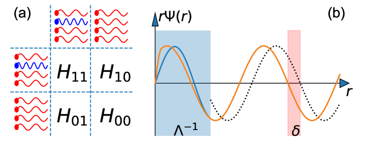
Figure 1: (a) Schematic plot of the partitioning of the Hamiltonian in the Fock space. Red (blue) points denote particles with momentum $|\bm{p}|\leq\Lambda^{\prime}$ ($\Lambda^{\prime}<|\bm{p}|\leq\Lambda$). (b) Schematic plot of radial wave functions for two-particle scattering. Red (Blue) lines denote the results calculated with $H$ ($H^{\prime})$. In asymptotic region $r\gg\Lambda^{-1}$ the two wave functions coincide and their difference from the free wave function (dotted line) gives the phase shift $\delta$.

Decoupling the soft and hard modes

Next we search for a unitary transformation that decouples space-$0^{\prime}$ and space-$1^{\prime}$ by eliminating the off-diagonal blocks of the Hamiltonian. For this purpose it is convenient to use the SRG flow equation[12, 13, 14]. This method involves a time-dependent unitary transformation $U(t)$ with $t\in[0,\infty)$. The transformed Hamiltonian $H(t)=U(t)^{-1}HU(t)$ follows a flow equation

$$i\partial_{t}H(t)=[\eta(t),H(t)],$$ (4)

where the operator $\eta(t)=i[H_{0}(t),H_{1}(t)]$ is a Hermite generator satisfying $i\partial_{t}U(t)=\eta(t)U(t)$. By computing the commutators explicitly we see that the flow defined by Eq.(4) amounts to a continuous evolution of the coefficients in Eq.(3). As long as $H_{1}(t)$ is not too large, we expect that the evolution suppresses the off-diagonal matrix elements in $H_{1}(t)$[24]. For $t\rightarrow\infty$ all terms in $H_{1}(t)$ vanish, the flow converges to a fixed point $H_{1}=\eta=0$ and $U(t)$ has a well-defined limit $U(\infty)$. The resulting Hamiltonian $H(\infty)=U(\infty)HU(\infty)^{-1}$ only contains diagonal terms. We can further apply a projector $P_{0^{\prime}}$ to space-$0^{\prime}$ to remove all terms containing both $\delta\Phi$ and $\delta\Phi^{\dagger}$. The final result $H^{\prime}=P_{0^{\prime}}H(\infty)P_{0^{\prime}}$ has the same form as Eq.(1) with all $\Lambda$ substituted by $\Lambda^{\prime}$ and all coefficients $m$, $C_{2}$, $C_{3}$, etc. updated to new values $m^{\prime}$, $C_{2}^{\prime}$, $C_{3}^{\prime}$, etc. Because $U(\infty)$ is unitary, the Hamiltonians $H^{\prime}$ and $H$ have exactly the same low-lying spectra.

Several important conclusions can be immediately drawn by inspecting the flow Eq.(4). First, as the generator $\eta(t)$ is a spatial integral of local operators consisting of equal numbers of creation and annilation opeartors, both $\eta(t)$ and the induced transformation $U(\infty)$ conserves the particle number $N$ and total momentum $\bm{P}$. Consequently, the single particle state $|\bm{p}\rangle=a_{\bm{p}}^{\dagger}|0\rangle$ with $|\bm{p}|<\Lambda^{\prime}$ is a common eigenvector of $H$ and $H^{\prime}$ with the same eigenvalue $E=p^{2}/2m$. It follows immediately that $m^{\prime}=m$ and other one-body terms like $\Phi^{\dagger}\nabla^{4}\Phi$ are strictly forbidden. Second, as $\eta(t)$ does not contain any long-range interaction, the transformation $U(\infty)$ is localized that $U(\infty)(|\phi_{1}\rangle\otimes|\phi_{2}\rangle)=U(\infty)|\phi_{1}\rangle\otimes U(\infty)|\phi_{2}\rangle$ where $|\phi_{1,2}\rangle$ are single- or many-particle wave packets separated by a distance much larger than $\Lambda^{-1}$ and the symbol $\otimes$ means the tensor product. For a typical reaction, the incoming (outgoing) state long before (after) the collision consists of well seperated clusters, each of which corresponds to a bound state of the Hamiltonian. Applying the transformation $U(\infty)$ to both the Hamiltonian and the incoming (outgoing) state, we transform $H$ to $H^{\prime}$ and the cluster wave functions from eigenvectors of $H$ to that of $H^{\prime}$ with the same binding energies, meanwhile the unitarity of $U(\infty)$ ensures the invariance of the $S$-matrix element. In Fig.1(b) we schematically compare the radial wave functions for a two-particle scattering process. The localized transformation $U(\infty)$ modifies the short-range wave function at $r\lesssim\Lambda^{-1}$ but preserves the asymptotic behaviour and the phase shift. For more complicated inelastic scattering and reactions, no such simple picture is available, but our arguments based on spatial locality is still tenable.

In summary, the existence of the localized unitary transformation $U(\infty)$ hinges on the presence of the direct-sum decomposition of the Fock space, which in turn relies on the usage of a universal single-particle regulator. In contrast, all recent chiral EFT constructions employ Galilean invariant regulators acting on relative momenta or even use different cutoffs for two- and three-body contact terms. Such regulators can not unambiguously and consistently separate the low- and high-momentum many-body Hilbert spaces. In these cases the RG invariance of the energy spectrum and $S$-matrix elements is not guaranteed by any known mechanism, and their cutoff-dependences are mostly uncontrollable.

The above procedure of lowering the cutoff can be repeated many times to generate the RG flows, which can then be analyzed using the whole toolbox of the conventional Wilsonian RG theory. We note that in most applications we do not need to explicitly compute hundreds of commutators in Eq.(4). It suffices to write down the most general Hamiltonian with the correct symmetries and regulators, then determine the LECs by matching to low-momentum observables.

RG invariance of the chiral EFT

The above discussions can be easily generalized to spin-1/2 Fermions like the nucleons. For a numerical demonstration, we take a simplified N²LO chiral Hamiltonian $H_{{\rm N2LO}}=K+V_{{\rm 2N}}+V_{{\rm 3N}}+V_{{\rm C}}+V_{{\rm OPEP}}$, where $K$ is the kinetic energy term, $V_{{\rm 2N}}$ and $V_{{\rm 3N}}$ are two- and three-body contact terms, $V_{{\rm C}}$ and $V_{{\rm OPEP}}$ are Coulomb and one-pion-exchange potentials, respectively[25]. In momentum space the two-nucleon force (2NF) is written as

$$V_{{\rm 2N}} = \left[B_{1}+B_{2}(\bm{\sigma}_{1}\cdot\bm{\sigma}_{2})+C_{1}q^{2}+C_{2}q^{2}(\bm{\tau}_{1}\cdot\bm{\tau}_{2})\right.$$

$$+C_{3}q^{2}(\bm{\sigma}_{1}\cdot\bm{\sigma}_{2})+C_{4}q^{2}(\bm{\sigma}_{1}\cdot\bm{\sigma}_{2})(\bm{\tau}_{1}\cdot\bm{\tau}_{2})$$

$$+C_{5}\frac{i}{2}(\bm{q}\times\bm{k})\cdot(\bm{\sigma}_{1}+\bm{\sigma}_{2})+C_{6}(\bm{\sigma}_{1}\cdot\bm{q})(\bm{\sigma}_{2}\cdot\bm{q})$$

$$\left.+C_{7}(\bm{\sigma}_{1}\cdot\bm{q})(\bm{\sigma}_{2}\cdot\bm{q})(\bm{\tau}_{1}\cdot\bm{\tau}_{2})\right]f_{{\rm 2N}}(p_{1},p_{2},p_{1}^{\prime},p_{2}^{\prime}),$$

where $\bm{\sigma}_{1,2}(\bm{\tau}_{1,2})$ are spin (isospin) matrices, $B_{i},C_{i}$ are low-energy constants (LECs), $\bm{p}$ ($\bm{p}^{\prime}$) is the relative incoming (outgoing) momentum, $\bm{q}=\bm{p}-\bm{p}^{\prime}$, $\bm{k}=(\bm{p}+\bm{p}^{\prime})/2$ are momentum transfers, $\bm{p}_{i}$ and $\bm{p}_{i}^{\prime}$ are the momenta of the individual nucleons. We adopt a single-particle regulator $f_{{\rm 2N}}=\prod_{i=1}^{2}g_{\Lambda}(p_{i})g_{\Lambda}(p_{i}^{\prime})$ where $g_{\Lambda}(p)=\exp(-p^{6}/2\Lambda^{6})$ is a soft cutoff function. Similarly, for the three-nucleon force (3NF) we take a simple contact term

$$V_{{\rm 3N}}=C_{{\rm 3N}}f_{{\rm 3N}}(p_{1},\cdots,p_{3}^{\prime})$$

where $C_{{\rm 3N}}$ is a LEC, $f_{{\rm 3N}}=\prod_{i=1}^{3}g_{\Lambda}(p_{i})g_{\Lambda}(p_{i}^{\prime})$ is a non-local single-particle regulator. The long-range pieces $V_{{\rm C}}$ and $V_{{\rm OPEP}}$ are both local potentials that do not depend on $\Lambda$. In what follows we solve the nuclear ground state energies using lattice EFT techniques[26, 27, 28, 29]. Particularly, we use Lanczos algorithm for ³H and the perturbative quantum Monte Carlo method[25] for ⁴He and ¹⁶O. The latter two are tightly bound doubly-magic nuclei for which the perturbation theory is most accurate. See Supplemental Material[24] for futher details of the interactions, methods and error quantifications.

Figure 2: (a) Dimensionless LECs as functions of $\Lambda$. (b) Triton binding energies calculated without (blue squares) and with (red triangles) the three-body force $V_{{\rm 3N}}$. The horizontal line denote the experimental value. (c) The same as Fig.b but for ⁴He. The Monte Carlo statistical errors are smaller than the symbols. The grey bands signify the estimated truncation errors from the perturbative QMC calculations[24]. (d) The same as Fig.c but for ¹⁶O.

Now we examine the Wilsonian RG flow by varying the cutoff $\Lambda$ from $400$ MeV to $250$ MeV with a constant interval of 25 MeV. For each value of $\Lambda$ we determine the LECs $B_{i}$, $C_{i}$ and $C_{{\rm 3N}}$ by fitting to the experimental neutron-proton scattering phase shifts for relative momenta below 200 MeV and the triton binding energy $E(^{3}$H)=$-8.482$ MeV[30, 31]. Note that the characteristic momentum in a typical nucleus can be estimated as $Q\sim\sqrt{mE_{B}}\approx 100$ MeV, where $E_{B}\approx 7$ MeV is the single-nucleon binding energy. To confirm that fitting with such low-momenta is enough, we have also fitted to the phase shifts up to $250$ MeV and found no meaningful improvement for the ground state calculations. According to the conventions in the RG analysis, the running LECs can be combined with powers of $\Lambda$ to form dimensionless coupling constants $\overline{B}_{i}=m\Lambda B_{i}$, $\overline{C}_{i}=m\Lambda^{3}C_{i}$ and $\overline{C}_{{\rm 3N}}=m\Lambda^{4}C_{{\rm 3N}}$. In Fig.2(a) we show the dependence of these parameters on $\Lambda$. Here we focus on the infrared asymptotic behaviour and can observe three different tendencies. While $\overline{B}_{1}$ is approximately a constant and $\overline{C}_{{\rm 3N}}$ increases, all other dimensionless LECs approach zero for $\Lambda\rightarrow 0$. In the language of the RG we can qualitatively say that $B_{1}$, $C_{{\rm 3N}}$ and all other LECs correspond to marginal, relevant and irrelevant operators, respectively.

Figure 3: The ground state energies of ⁴He and ¹⁶O calculated with $H_{{\rm N2LO}}$ (squares) and $H_{{\rm N3LO}}$ (triangles). The results without the 3NF are denoted as open symbols. The dashed line is for guiding the eyes. The star denotes the experimental values. The inset schematizes two typical RG flows in the parameter space. $\overline{C}_{{\rm 3N}}$ and $\overline{D}_{i}$ corresponds to the 3NF and an irrelevant operator, respectively. As $\Lambda$ is lowered, two different theories with $\overline{D}_{i}=0$ and $\overline{D}_{i}\neq 0$ flow to the same low-momentum EFT.

In Fig.2(b-d) we show the binding energies of ³H, ⁴He and ¹⁶O calculated with running $\Lambda$ and the corresponding LECs. To see the effects of the 3NF we display the results with and without the 3NF as triangles and squares, respectively. The binding energies without the 3NF show appreciable $\Lambda$-dependence and vary by about $20\%$ for the considered interval of $\Lambda$. For the calculations with the 3NF, the ³H energy is fitted to and always equals to the experimental value, whereas both the ⁴He and ¹⁶O energies are predictions. Surprisingly, the simple 3NF determined in ³H cancels most of the $\Lambda$-dependence in ⁴He and ¹⁶O energies and significantly improves the description of both experimental values. In particular, for $\Lambda\geq 300$ MeV the ¹⁶O energy converges to the experimental value with a discrepancy smaller than $2$ MeV. Note that our calculation has no adjustable parameter other than the LECs fitted to two- and three-body observables, thus the predictions are really model-independent.

The remaining $\Lambda$-dependence has multiple sources. For instance, we have employed a soft cutoff function which does not completely exclude the high-momentum subspace[33, 32]. Another important source is the ommision of the contact terms that explicitly violate the Galilean invariance[34]. Generally, these effects scale as negative powers of $\Lambda$, thus to extract unambiguous predictions we need to make an extrapolation using multiple values of $\Lambda$. This can be clearly seen for the convergence pattern of $E(^{4}$He$)$ in Fig.2(c). Following the Symanzik improvement program[35, 36] in the lattice QCD, we can also add irrelavent operators to absorb these regulator artifacts. Fortunately, in our cases such RG-invariance breaking effects are sufficiently weak and we leave it as is.

Now we check whether the agreement with the experiments persists for higher-order interactions. We fix $\Lambda$ to 400 MeV that minimizes the regulator artifacts, add fifteen two-body contact terms at $\mathcal{O}(Q^{4})$ to the Hamiltonian and refit all LECs using the same prescription as for $H_{{\rm N2LO}}$. We denote the resulting Hamiltonian as $H_{{\rm N3LO}}$[24]. Note that $H_{{\rm N2LO}}$ and $H_{{\rm N3LO}}$ give nearly the same phase shifts below 200 MeV and the same triton binding energy. In Fig.3 we plot $E$(⁴He) versus $E$(¹⁶O) predicted by both Hamiltonians. We also display the results without the 3NF as open symbols. The star denotes the experimental values. We see that the ⁴He and ¹⁶O energies are highly correlated that their energy corrections from the higher-order 2NF can be canceled simultaneously by adjusting the 3NF. We also found that the ³H and ⁴He energies are correlated as expected by the Tjon line[37]. Thus we conclude that at N³LO a single 3NF is also enough for reproducing all three binding energies.

The phenomena that a simple pattern emerges from complex underlying interactions is known as the universality. Famous examples in nuclear physics are the Tjon line[37] and Coester line[38]. Similar to the cases in thermodynamics, such emergence behaviour in nuclear physics can also be understood via the RG transformations. In the inset of Fig.3 we schematize the Wilsonian RG flows of two Hamiltonians starting with and without a typical 2NF at $\mathcal{O}(Q^{4})$. The 2NF is represented by a single parameter $\overline{D}_{i}$. Note that $\overline{C}_{{\rm 3N}}$ and $\overline{D}_{i}$ correspond to relevant and irrelevant operators, respectively. Following the Wilsonian RG analysis near a fixed point, for any value of $\overline{D}_{i}$ we can always adjust $\overline{C}_{{\rm 3N}}$ to make the RG flow converge to the same low-momentum EFT located on a low-dimensional invariant surface. These RG flows are independent of the nucleon number and induce the observed correlations between the binding energies.

Summary and perspective

We present a general framework for buiding RG invariant EFTs. In brief, our method is a non-relativistic counterpart of the Wilsonian RG theory. The only requirement is to regulate all single-particle momenta with the same cutoff. It applies for non-perturbative as well as perturbative EFTs. The RG flows can be calculated explicitly from the operator commutators. The first application of this paradigm to realistic chiral forces yields promising results. Our findings suggest that the RG invariance might be realized at much lower orders and smaller cutoffs than previously expected. Its consequences on other $\chi$EFT calculations are being examined. As the rigidity of the predictions is guaranteed by the RG invariance, fine-tuning is not allowed and we expect that the discrepancies to the experiments would signify the real missing physics such as the medium effects.

Supplemental Material

In the main text we present a numerical demonstration using the realistic chiral interactions. Here we present the details of the chiral interaction, the many-body methods and the error quantifications. Note that some of the materials have already been given in Ref.[1] and the supplemental materials of Ref.[2]. For completeness we also include them here. We also give a proof of the convergence of the flow equation.

Nuclear chiral interactions

Up to N²LO the form of the interaction is exactly the same as that we used in Ref.[2]. For contact terms we employ the semi-local operator basis that contains isospin dependent terms proportional to $\bm{\tau}_{1}\cdot\bm{\tau}_{2}$. In this form, the contact terms are mostly seperable and can be written as products of one-body density operators, which is amenable to quantum Monte Carlo simulations. We note that similar constructions have already been used for the N²LO Green’s function Monte Carlo calculations[4, 3]. In addition, we also present the fifteen semi-local N³LO contact terms.

In momentum space the contact terms up to $\mathcal{O}(Q^{4})$ are written as

$$V_{Q^{0}} = B_{1}+B_{2}(\bm{\sigma}_{1}\cdot\bm{\sigma}_{2})$$

$$V_{{\rm Q^{2}}} = C_{1}q^{2}+C_{2}q^{2}(\bm{\tau}_{1}\cdot\bm{\tau}_{2})+C_{3}q^{2}(\bm{\sigma}_{1}\cdot\bm{\sigma}_{2})+C_{4}q^{2}(\bm{\sigma}_{1}\cdot\bm{\sigma}_{2})(\bm{\tau}_{1}\cdot\bm{\tau}_{2})$$

$$+C_{5}\frac{i}{2}(\bm{q}\times\bm{k})\cdot(\bm{\sigma}_{1}+\bm{\sigma}_{2})+C_{6}(\bm{\sigma}_{1}\cdot\bm{q})(\bm{\sigma}_{2}\cdot\bm{q})+C_{7}(\bm{\sigma}_{1}\cdot\bm{q})(\bm{\sigma}_{2}\cdot\bm{q})(\bm{\tau}_{1}\cdot\bm{\tau}_{2})$$

$$V_{{\rm Q^{4}}} = D_{1}q^{4}+D_{2}q^{4}(\bm{\tau}_{1}\cdot\bm{\tau}_{2})+D_{3}q^{4}(\bm{\sigma}_{1}\cdot\bm{\sigma}_{2})+D_{4}q^{4}(\bm{\sigma}_{1}\cdot\bm{\sigma}_{2})(\bm{\tau}_{1}\cdot\bm{\tau}_{2})$$ (5)

$$+D_{5}q^{2}(\bm{\sigma}_{1}\cdot\bm{q})(\bm{\sigma}_{2}\cdot\bm{q})+D_{6}q^{2}(\bm{\sigma}_{1}\cdot\bm{q})(\bm{\sigma}_{2}\cdot\bm{q})(\bm{\tau}_{1}\cdot\bm{\tau}_{2})+D_{7}q^{2}k^{2}$$

$$+D_{8}q^{2}k^{2}(\bm{\sigma}_{1}\cdot\bm{\sigma}_{2})+D_{9}(\bm{q}\cdot\bm{k})^{2}+D_{10}(\bm{q}\cdot\bm{k})^{2}(\bm{\sigma}_{1}\cdot\bm{\sigma}_{2})$$

$$+D_{11}\frac{i}{2}q^{2}(\bm{q}\times\bm{k})\cdot(\bm{\sigma}_{1}+\bm{\sigma}_{2})+D_{12}\frac{i}{2}q^{2}(\bm{q}\times\bm{k})\cdot(\bm{\sigma}_{1}+\bm{\sigma}_{2})(\bm{\tau}_{1}\cdot\bm{\tau}_{2})$$

$$+D_{13}k^{2}(\bm{\sigma}_{1}\cdot\bm{q})(\bm{\sigma}_{2}\cdot\bm{q})+D_{14}q^{2}(\bm{\sigma}_{1}\cdot\bm{k})(\bm{\sigma}_{2}\cdot\bm{k})$$

$$+D_{15}\left[(\bm{q}\times\bm{k})\cdot\bm{\sigma}_{1}\right]\left[(\bm{q}\times\bm{k})\cdot\bm{\sigma}_{2}\right],$$

where $B_{1-2}$, $C_{1-7}$ and $D_{1-15}$ are low-energy constants (LECs), $\bm{q}=\bm{p}^{\prime}-\bm{p}$ and $\bm{k}=(\bm{p}+\bm{p}^{\prime})/2$ are momentum transfers, $\bm{\sigma}_{1,2}$ and $\bm{\tau}_{1,2}$ are spin and isospin Pauli matrices, respectively. Due to wave function anti-symmetrization this choice of operators is not unique. For convenience in lattice calculations we choose the semi-local basis in Eq.(5) that minimizes the dependence on $\bm{k}$. In Ref.[5] it was pointed out that at order $Q^{4}$ there are two redundant operators in reproducing the N-N phase shifts. This correspond to the fact that the operators attached to $D_{9}$ and $D_{10}$ vanish for on-shell momenta $|\bm{p}|=|\bm{p}^{\prime}|$.

For all two-body contact terms we introduce a non-local regulator $f_{{\rm 2N}}=\exp[-\sum_{i=1}^{2}\left(p_{i}^{6}+p_{i}^{\prime 6}\right)/(2\Lambda^{6})]$, where $\bm{p}_{1,2}$ and $\bm{p}_{1,2}^{\prime}$ are incoming and outgoing single particle momenta, respectively. Comparing with the form used in Ref.[2], here we insert an extra factor $2$ before $\Lambda$ for convenience. For two colliding nuclei in the center of mass frame, we have the relative momenta $\bm{p=\bm{p}_{1}=-\bm{p}_{2}}$ and $\bm{p}^{\prime}=\bm{p}_{1}^{\prime}=-\bm{p}_{2}^{\prime}$, thus $f_{{\rm 2N}}=\exp(-(p^{6}+p^{\prime 6})/\Lambda^{6})$ reduces to the non-local regulator extensively used in chiral EFT constructions[6, 7]. However, for many-body systems, our regulator is imposed on single-particle momenta rather than relative momenta, thus gives different predictions even though the two-body LECs are the same.

In the main text we include a long-range one-pion-exchange potential (OPEP) $V_{{\rm OPEP}}$ in the chiral interactions. Here we give the details. In momentum space we have

$$V_{{\rm OPEP}}=-\frac{g_{A}^{2}f_{\pi}(q^{2})}{4F_{\pi}^{2}}\left[\frac{(\bm{\sigma}_{1}\cdot\bm{q})(\bm{\sigma}_{2}\cdot\bm{q})}{q^{2}+M_{\pi}^{2}}+C_{\pi}^{\prime}\bm{\sigma}_{1}\cdot\bm{\sigma}_{2}\right](\bm{\tau}_{1}\cdot\bm{\tau}_{2}),$$

where $g_{A}=1.287$, $F_{\pi}=92.2$ MeV, $M_{\pi}=134.98$ MeV are the axial-vector coupling constant, pion decay constant and pion mass, respectively. The OPEP is regulated with a local exponential regulator $f_{\pi}(q^{2})=\exp[-(q^{2}+M_{\pi}^{2})/\Lambda_{\pi}^{2}]$ with $\Lambda_{\pi}$ fixed to $300$MeV. We also tested other values of $\Lambda_{\pi}$ and found similar results as presented here. The constant $C_{\pi}^{\prime}$ is defined as

$$C_{\pi}^{\prime} =\frac{1}{3\Lambda_{\pi}^{3}}\Biggl{[}\Lambda_{\pi}(\Lambda_{\pi}^{2}-2M_{\pi}^{2})+2\sqrt{\pi}M_{\pi}^{3}\exp(\frac{M_{\pi}^{2}}{\Lambda_{\pi}^{2}}){\rm erfc}(\frac{M_{\pi}}{\Lambda_{\pi}})\Biggr{]}.$$

The term proportional to $C_{\pi}^{\prime}$ is a counterterm introduced to remove the short-range singularity from the OPEP[5]. We note that the OPEP regulated in this way is soft and adaptive to perturbative calculations[2].

For the three-body force at N²LO we adopt a simple 3N contact term with Wigner SU(4) symmetry[8],

$$V_{{\rm 3N}}=C_{{\rm 3N}}f_{{\rm 3N}}(p_{1},p_{2},\cdots,p_{3}^{\prime}),$$

where $C_{{\rm 3N}}$ is a LEC, $f_{{\rm 3N}}=\exp[-\sum_{i=1}^{3}\left(p_{i}^{6}+p_{i}^{\prime 6}\right)/(2\Lambda^{6})]$ is a seperable single-particle regulator. Note that we use the same soft cutoff functions and the same value of $\Lambda$ in $f_{{\rm 2N}}$ and $f_{{\rm 3N}}$.

Besides the nuclear force we also include a static Coulomb force,

$$V_{{\rm C}}=:\frac{\alpha}{2}\int d^{3}\bm{r}_{1}d^{3}\bm{r}_{2}\frac{\rho_{p}(\bm{r}_{1})\rho_{p}(\bm{r}_{2})}{|\bm{r}_{1}-\bm{r}_{2}|}:$$

where $\rho_{p}$ is the total proton density, $\alpha=1/137$ is the fine structure constant.

We implement the Hamiltonian on a cubic lattice using fast Fourier transform and determine the LECs $B_{i}$, $C_{i}$, $D_{i}$ and $C_{{\rm 3N}}$ by fitting to the low-energy NN phase shifts, mixing angles and triton energy. The method is based on Ref.[9]. We decompose the scattering waves on the lattice into different partial waves, then employ the real and complex auxiliary potentials to extract the asymptotic radial wave functions. We follow the conventional procedure for fitting the LECs in the continuum[10]. We first determine the spectroscopic LECs for each partial wave, then the $B_{i}$, $C_{i}$ and $D_{i}$ can be obtained by solving the linear equations.

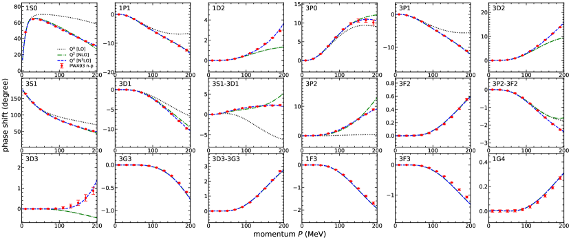
Figure 4: Neutron-proton phase shifts calculated with the momentum cutoff $\Lambda$=400 MeV. Dotted, dash-dotted and dashed lines denote the LO, NLO and N³LO results, respectively. Red circles with error bars show the empirical values[11].

In this work we consider NN scattering up to a relative momentum $P_{{\rm rel}}=200$ MeV. In Fig.4 we show the calculated phase shifts for $\Lambda=400$ MeV. The dotted, dash-dotted and dashed lines denote the results at LO, NLO and N³LO, respectively. The red dots with error bars are empirical values from the Nijmegen partial wave analysis (NPWA)[11].

In principle the $\pi$-$N$ coupling $g_{A}$ should also run with $\Lambda$. However, as the OPEP does not explicitly contain $\Lambda$, we expect that the dependence is rather weak. We confirm this point by refitting the LECs with different values of $g_{A}$. We found that $g_{A}=1.287$ always approximately gives the best fit for $\Lambda=250\simeq 400$ MeV and conclude that the OPEP do not evolve.

Compared with other high-precision N³LO chiral interactions, our construction lacks the two-pion exchange potentials (TPEP). The reason is that for momentum much lower than $2M_{\pi}\approx 270$ MeV, the TPEP can be approximately absorbed into the contact terms and discarded. This point can be clearly seen by inspecting the peripheral partial waves like ${}^{3}F_{3}$ or ${}^{1}G_{4}$ in Fig.4. These partial waves are solely determined by the OPEP. The good reproduction of the empirical values makes it unnecessary to include the TPEP in this momentum interval. This argument also applies to three-pion exchange potentials.

In the three-body sector we also ommitted the one-pion-exchange three-body force. It was long known that the two three-body terms at N²LO can not be uniquely fixed with ³H and ⁴He binding energies which are highly correlated[12, 13]. In this work we also found similar correlation between the ⁴He and ¹⁶O energies for the three-body forces. The situation is quite similar to the case of N³LO contact terms. Thus we still can not distinguish the two three-body forces even with the ¹⁶O binding energy as an additional input. This finding can be contrasted with the recent practices of adapting the three-body forces to many-body observables. We conjecture that the difference is related to the different regulators and need further investigations.

Finally, the RG transform induces additional terms such as $Q^{2}$, $Q^{2}(\bm{\sigma}_{1}\cdot\bm{\sigma}_{2})$, $(\bm{Q}\cdot\bm{\sigma}_{1})(\bm{Q}\cdot\bm{\sigma}_{2})$ etc., where $\bm{Q}=\bm{p}_{1}+\bm{p}_{2}=\bm{p}_{1}^{\prime}+\bm{p}_{2}^{\prime}$ is the center of mass momentum. For a full RG invariance calculation we need to include all of them in the expansion of the EFT Hamiltonian, then fit the corresponding LECs to restore the Galillean invariance in each partial waves. This is as difficult as fitting the normal LECs and only has been performed for the leading order terms[14]. Fortunately, since the Galillean invariance breaking effects originate from the single-particle regulator imposed at a large momentum $\Lambda$, the LECs for these Galillean-invariance-restoration (GIR) terms scale as negative powers of $\Lambda$ and decay to zero for large $\Lambda$. For example, the calculations in the main text simply ommit all GIR terms and we can expect that the results converge as $\mathcal{O}(\Lambda^{-2})$ for large $\Lambda$. By including the GIR terms at $\mathcal{O}(Q^{2})$ we can accelerate the convergence speed to $\mathcal{O}(\Lambda^{-4})$. This procedure is a non-relativistic counterpart of the Symanzik improvement for the lattice QCD action[15, 16], where irrelevant operators proportional to $a^{2}$, $a^{4}$, etc., are added to the QCD Lagrangian to absorb the lattice artifacts, where $a$ is the lattice spacing. The most notable difference is that in an EFT we can not take the limit $\Lambda\rightarrow\infty$ as new physics may emerge at certain hard scale where the EFT breaks down.

Perturbative quantum Monte Carlo method

In this work we solve the ⁴He and ¹⁶O ground state energies using the perturbative quantum Monte Carlo method [2]. The starting point is a zeroth order Hamiltonian respecting the Wigner SU(4) symmetry[8]. While the SU(4) Hamiltonian in Ref.[2] is designed for lattice spacing $a=1.32$ fm, in this work we use a finer lattice with $a=1.0$ fm and slightly adjust the form of the interaction. On a pariodic $L^{3}$ cube with lattice coordinates $\bm{n}=(n_{x},n_{y},n_{z})$, the zeroth order Hamiltonian is

$$H_{0}=K+\frac{1}{2}C_{{\rm SU4}}\sum_{\bm{n}}:\tilde{\rho}^{2}(\bm{n}):,$$ (6)

where $K$ is the kinetic energy term with nucleon mass $m=938.92$ MeV and the $::$ symbol indicate normal ordering. The smeared density operator $\tilde{\rho}(\bm{n})$ is defined as

$$\tilde{\rho}(\bm{n})=\sum_{i}\tilde{a}_{i}^{\dagger}(\bm{n})\tilde{a}_{i}(\bm{n})+s_{L}\sum_{|\bm{n}^{\prime}-\bm{n}|=1}\sum_{i}\tilde{a}_{i}^{\dagger}(\bm{n}^{\prime})\tilde{a}_{i}(\bm{n}^{\prime}),$$

where $i$ is the joint spin-isospin index and the smeared annihilation and creation operators are defined as

$$\tilde{a}_{i}(\bm{n})=\sum_{\bm{n}^{\prime}}g(|\bm{n}-\bm{n}^{\prime}|)a_{i}(\bm{n}^{\prime}),$$

where $g(r)=(\Lambda_{NL}/\sqrt{2\pi})^{3}\exp(-\Lambda_{NL}^{2}r^{2}/2)$ is a Gaussian smearing function. The summation over the spin and isospin implies that the interaction is SU(4) invariant. The parameter $s_{L}$ controls the strength of the local part of the interaction, while $\Lambda_{NL}$ controls the strength of the non-local part of the interaction. Here we include both kinds of smearing. Both $s_{L}$ and $\Lambda_{NL}$ have an impact on the range of the interactions. The parameter $C_{{\rm SU4}}$ gives the strength of the two-body interactions. In this work we use the parameter set $C_{{\rm SU4}}=-3.7912\times 10^{-5}$ MeV^-2, $s_{L}=0.182$ and $\Lambda_{NL}=300$ MeV. These parameters together with a properly chosen three-body force reproduce the binding energies of light nuclei.

In auxiliary field Monte Carlo calculations, the SU(4) Hamiltonian in Eq.(6) generates the same auxiliary fields for spin-up and spin-down particles. For even-even nuclei like ⁴He and ¹⁶O, the determinant from the wave function antisymmmetrization can be factorized into a product of identical determinants, which is positive definite. In such a sign-problem-free scenario the Monte Carlo simulation can be very accurate[1]. However, the realistic interactions usually break the SU(4) symmetry and induce severe sign problem, causing large statistical errors. To solve this problem, we rewrite the full Hamiltonian $H$ as a sum of the SU(4) symmetric Hamiltonian $H_{0}$ and a residual term $\delta H$, then use Monte Carlo techinques to simulate $H_{0}$ non-perturbatively and incoorporate $\delta H$ using the 2nd order perturbation theory. In this way we can largely suppress the sign problem at the price of introducing minor perturbative truncation errors[2]. In this work $H$ can be either the realistic chiral Hamiltonian $H_{{\rm N2LO}}$ fitted with $\Lambda=250\simeq 400$ MeV or $H_{{\rm N3LO}}$ fitted with $\Lambda=400$ MeV.

Error quantifications

For a solid demonstration, we need to estimate the numerical errors due to the many-body methods. Note that we only consider the errors from solving a given Hamiltonian. The uncertainties from truncating the chiral Hamiltonian at a given order are reflected by the breaking of the RG invariance, which has been discussed in the main text.

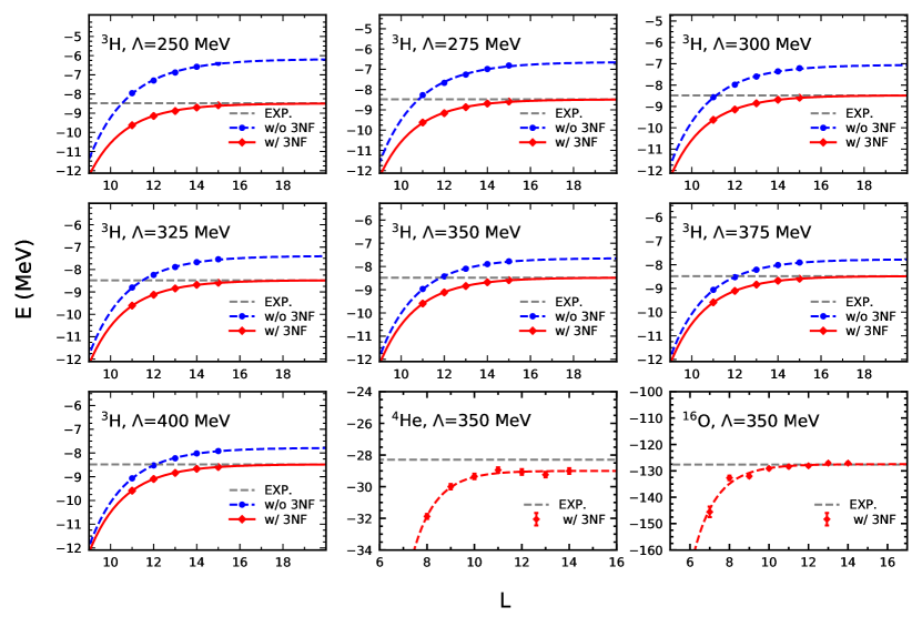
Figure 5: The ground state energies of ³H, ⁴He and ¹⁶O calculated with different box size $L$. The circles and diamonds denote the results with and without the three-body force, respectively. The dashed and solid lines are fitted curves for extrapolating to the infinite volume limit. The horizontal lines are corresponding experimental values. The errorbars for ⁴He and ¹⁶O denote the Monte Carlo statistical errors.

Continuum limit

In this work we fix the lattice spacing to $a=1.0$ fm. This corresponds to a momentum cutoff $\Lambda_{a}=\pi/a\approx 620$ MeV. When we consider a Hamiltonian regulated by an extra regulator with a cutoff $\Lambda=250\simeq 400$ MeV $\ll\Lambda_{a}$, the spatial lattice is invisible to the particles. In other words, we can further take the continuum limit $a\rightarrow 0$ or $\Lambda_{a}\rightarrow\infty$ to eliminate the discretization errors. In this sense the lattice is used as a numerical tool for solving the quantum many-body problem and has no physical meaning. What is physical relevance is the cutoff $\Lambda$ defined in the spatial continuum. Thus our results can be immediately benchmarked using other many-body algorithms designed for general Hamiltonians, e.g., no-core shell model[17] or IM-SRG method[18]. This setting is quite different from the recent lattice EFT calculations, where the lattice was explicitly used as the momentum regulator and the lattice spacing must be kept finite throughout.

Infinite volume limit

To make a precision fit for the three-body parameter $C_{{\rm 3N}}$, we calculate the triton binding energy by directly diagonalizing the lattice Hamiltonian using the Lanczos method. As this method becomes expensive for large volumes, we use small box sizes $L=11\simeq 15$ and extrapolate the results to $L\rightarrow\infty$. We measure the box size in unit of the lattice spacing. In Fig.5 we show the triton binding energies calculated with and without the three-body force as functions of $L$. The dashed and solid lines are fitted curves using the ansatz for three particles in the unitary limit[19],

$$E(L)=E(\infty)+\mathcal{A}\exp(2\kappa L/\sqrt{3})/(\kappa L)^{3/2}$$

with $\kappa=\sqrt{-mE(\infty)}$, $m$ is the nucleon mass. We ensure that all triton energies with the three-body force converge to the experimental value $E(^{3}$H)=$-8.482$ MeV. In Fig.2b of the main text, the displayed triton energies are extrapolated values.

For ⁴He we use the Monte Carlo method and take $L=12$ for all calculations. For ¹⁶O we take $L=11$. For saving the computational resources, we only examine the convergence patterns for $\Lambda=350$ MeV. The results are also displayed in Fig.5. Clearly the results with $L=12$ and $11$ are sufficiently close to the infinite volume limit.

Perturbative truncation errors

For ⁴He and ¹⁶O energies we employed the 2nd order perturbation theory[2]. The errors from truncating the perturbative series account for most of the numerical errors. Following Ref.[2], we roughly estimate the truncation errors by varying the zeroth order Hamiltonian $H_{0}$. If the perturbative series converge and we can calculate up to infinite orders, the results will be determined by $H$ and independent of $H_{0}$. Thus any dependence on $H_{0}$ is a signature of truncating the series at a finite order. For all Monte Carlo calculations in the main text, we perform the simulation using three different $H_{0}$ with $C_{{\rm SU4}}$ multiplied by $0.9$, $1.0$ and $1.1$, respectively. We found that the eigenvalues of $H_{0}$ vary by about 20% for different values of $C_{{\rm SU4}}$. However, after including $\delta H=H-H_{0}$ using the perturbative QMC method, we found that the energies are almost constants against $C_{{\rm SU4}}$. In Fig.2 of the main text we plot the uncertainties due to the variation of $C_{{\rm SU4}}$ with the grey bands.

Convergence of the flow equation

Below the flow Eq.(4) in the main text we claim that it converges to the fixed point $H_{1}=\eta=0$ as long as $H_{1}$ is small. Here we give a more detailed derivation. The proof follows the derivation of the $V_{lowk}$ potential[20] with minor modifications.

In the main text we write the Hamiltonian as $H=H_{0}+H_{1}$ and show that $H_{0}$ is block-diagonal. Formally we can write

$$H_{0}=\left(\begin{array}[]{cc}A_{0}\\ &A_{1}\end{array}\right),\qquad H_{1}=\left(\begin{array}[]{cc}\epsilon&b\\ b^{\dagger}\end{array}\right),$$

where $A_{0}$, $A_{1}$ and $\epsilon$ are Hermite matrices. Then we can calculate the generator as

$$i\eta=[H_{0},H_{1}]=\left(\begin{array}[]{cc}A_{0}\epsilon-\epsilon A_{0}&A_{0}b-bA_{1}\\ A_{1}b^{\dagger}-b^{\dagger}A_{0}\end{array}\right),$$

then substituting $i\eta$ into the flow equation we get

$$\frac{dH}{dt}=[i\eta,H]=[\left(\begin{array}[]{cc}A_{0}\epsilon-\epsilon A_{0}&A_{0}b-bA_{1}\\ A_{1}b^{\dagger}-b^{\dagger}A_{0}\end{array}\right),\left(\begin{array}[]{cc}A_{0}+\epsilon&b\\ b^{\dagger}&A_{1}\end{array}\right)].$$

Taking the $(1,2)$ matrix element we get

$$\frac{db}{dt}=(A_{0}\epsilon-\epsilon A_{0})b+(A_{0}b-bA_{1})A_{1}-(A_{0}+\epsilon)(A_{0}b-bA_{1})\approx 2A_{0}bA_{1}-bA_{1}^{2}-A_{0}^{2}b,$$

where we only keep terms linear in $b$ or $\epsilon$. These terms are from $H_{1}$ which contains at least one $\delta\Psi$ or $\delta\Psi^{\dagger}$. When $\Lambda^{\prime}$ is close to $\Lambda$ these terms are much smaller than $\Psi$ and $\Psi^{\dagger}$, thus can be treated as infinitesimals compared with $A_{0}$ and $A_{1}$. Then we can calculate the derivative of the positive definite expression,

$$\frac{d}{dt}{\rm Tr}(b^{\dagger}b) ={\rm Tr}(\frac{db^{\dagger}}{dt}b+b^{\dagger}\frac{db}{dt})=2{\rm Tr}(2A_{1}b^{\dagger}A_{0}b-A_{1}^{2}b^{\dagger}b-bb^{\dagger}A_{0}^{2})$$

$$=-2{\rm Tr}[(A_{0}b-bA_{1})^{\dagger}(A_{0}b-bA_{1})]\leq 0,$$

thus the off-diagonal blocks always decreases in the course of the evolution. As every term in $H_{1}$ has non-zero matrix elements in the off-diagonal block $b$ or $b^{\dagger}$, eliminating $b$ and $b^{\dagger}$also means getting rid of $H_{1}$.

References

- [1] Bing-Nan Lu, Ning Li, Serdar Elhatisari, Dean Lee, Evgeny Epelbaum and Ulf-G. Meiï¿œner, Phys. Lett. B 797, 134863 (2019)
- [2] Bing-Nan Lu, Ning Li, Serdar Elhatisari, Yuan-Zhuo Ma, Dean Lee and Ulf-G. Meiï¿œner, Phys. Rev. Lett. 128, 242501 (2022)
- [3] D. Lonardoni, J. Carlson, S. Gandolfi, J. E. Lynn, K. E. Schmidt, A. Schwenk and X. B. Wang, Phys. Rev. Lett. 120, 122502 (2018)
- [4] A. Gezerlis, I. Tews, E. Epelbaum, S. Gandolfi, K. Hebeler, A. Nogga and A. Schwenk, Phys. Rev. Lett. 111, 032501 (2013)
- [5] P. Reinert, H. Krebs and E. Epelbaum, Eur. Phys. J. A 54, 86 (2018)
- [6] E. Epelbaum, H.-W. Hammer and Ulf-G. Meiï¿œner, Rev. Mod. Phys. 81, 1773 (2009)
- [7] R. Machleidt and D. R. Entem, Phys. Rept. 503, 1 (2011)
- [8] E. Wigner, Phys. Rev. 51, 106 (1937).
- [9] Bing-Nan Lu, Timo A. Lï¿œhde, Dean Lee and Ulf-G. Meiï¿œner, Phys. Lett. B 760, 309 (2016)
- [10] E. Epelbaum, W. Glï¿œckle and Ulf-G. Meiï¿œner, Nucl. Phys. A 747, 362 (2005)
- [11] V. G. J. Stoks, R. A. M. Klomp, M. C. M. Rentmeester, and J. J. de Swart, Phys. Rev. C 48, 792 (1993)
- [12] L. Platter, H.-W. Hammer and U.-G. Meiï¿œner, Phys. Lett. B 607, 254 (2005)
- [13] Nico Klein, Serdar Elhatisari, Timo A. Lï¿œhde, Dean Lee and Ulf-G. Meiï¿œner, Eur. Phys. J. A 54, 121 (2018)
- [14] Ning Li, Serdar Elhatisari, Evgeny Epelbaum, Dean Lee, Bing-Nan Lu and Ulf-G. Meiï¿œner, Phys. Rev. C 99, 064001 (2019)
- [15] K. Symanzik, Nucl. Phys. B 226, 187 (1983)
- [16] K. Symanzik, Nucl. Phys. B 226, 205 (1983)
- [17] B. R. Barrett, P. Navratil and J. P. Vary, Prog. Part. Nucl. Phys. 69, 131 (2013)
- [18] H. Hergert, S. K. Bogner, T. D. Morris, A. Schwenk and K. Tsukiyama, Phys. Rept. 621, 165 (2016)
- [19] U.-G. Meiï¿œner, G. Rios and A. Rusetsky, Phys. Rev. Lett. 114, 091602 (2015)
- [20] S. K. Bogner, R. J. Furnstahl and A. Schwenk, Prog. Part. Nucl. Phys. 65, 94 (2010)