On the interplay between pricing, competition and QoS in ride-hailing

Abstract

We analyse a non-cooperative game between two competing ride-hailing platforms, each of which is modeled as a two-sided queueing system, where drivers (with a limited level of patience) are assumed to arrive according to a Poisson process at a fixed rate, while the arrival process of (price-sensitive) passengers is split across the two platforms based on Quality of Service (QoS) considerations. As a benchmark, we also consider a monopolistic scenario, where each platform gets half the market share irrespective of its pricing strategy. The key novelty of our formulation is that the total market share is fixed across the platforms. The game thus captures the competition between the platforms over market share, with pricing being the lever used by each platform to influence its share of the market. The market share split is modeled via two different QoS metrics: (i) probability that an arriving passenger gets a ride (driver availability), and (ii) probability that an arriving passenger gets an acceptable ride (driver availability and acceptable price). The platform aims to maximize the rate of revenue generated from matching drivers and passengers.

In each of the above settings, we analyse the equilibria associated with the game in a certain limiting regime, where driver patience is scaled to infinity. We also show that these equilibria remain relevant in the more practically meaningful ‘pre-limit,’ where drivers are highly (but not infinitely) patient. Interestingly, under the second QoS metric, we show that for a certain range of system parameters, no pure Nash equilibrium exists. Instead, we demonstrate a novel solution concept called an equilibrium cycle, which has interesting dynamic connotations. Our results highlight the interplay between competition, passenger-side price sensitivity, and passenger/driver arrival rates.

1 Introduction

The ride-hailing industry, exemplified by platforms like Uber, Lyft, and Ola, has gained tremendous popularity and growth in recent years. These platforms operate as two-sided matching systems, where passengers in need of a ride and willing drivers are matched in real time. The scale of these matching platforms is remarkable, with OLA alone boasting over 1.5 million drivers across 250 cities in India [1].

In the ride-hailing space, we see strategic behavior on part of passengers as well as platforms. On one hand, passengers choose which platform to use based on not just its pricing, but also its (history of) driver availability. (Indeed, today, technology has considerably cut the friction associated with switching between platforms.) On the other hand, platforms seek to maximize their revenues while competing with one another for market share; each platform must optimize its pricing to balance its market share and its revenue per-ride. It is this interplay between pricing, competition, market segmentation and QoS that we seek to analyse in this paper.

Although there has been some recent research on competing (two-sided) matching platforms, most studies overlook the crucial queueing aspects that are inherent in practical ride-hailing systems, including random passenger/driver arrivals, the likelihood of driver availability, as well as random transit durations. Moreover, most existing studies rely on numerical computations of the system equilibria to draw their insights on impact of the strategic interaction between competing platforms (we provide a detailed review of the related literature later in this section). This paper aims to bridge this gap by formally analyzing a non-cooperative game between two ride-hailing platforms that compete for market share. The platforms compete via their pricing strategies, to serve a passenger base which is both impatient as well as price sensitive.

Specifically, we assume symmetric platforms, a single geographical zone of operation, and static (not state-dependent) pricing. The market share of each platform is modeled as a Wardrop equilibrium [2] (defined in terms of a certain QoS metric). We then characterize the equilibria associated with this game, approximating the payoff functions along a certain scaling regime (where driver impatience is diminishing). These equilibria shed light on the influence of passenger price sensitivity and passenger/driver arrival rates on pricing, platform surplus, and passenger QoS in the presence of inter-platform competition.

Our main contributions are as follows:

• We model each platform as a BCMP network ([4]), admitting a product form stationary distribution. This model captures passenger-side price sensitivity, queueing (and impatience) of drivers, and transit times. (This BCMP modeling approach is quite powerful, and also allows for state-dependent pricing and probabilistic routing across multiple zones, though these features are not used in our analysis here.)

• For benchmarking (i.e., to capture the impact of inter-platform competition), we first consider a monopolistic scenario, where each platform gets half the market share, irrespective of its pricing strategy. We characterize the optimal pricing strategy of each platform under a certain limiting regime where driver patience grows unboundedly—we refer to this scaling regime as the Infinite Driver Patience ($\mathsf{IDP}$) regime.

• To capture competition between platforms, we model market share bifurcation between the platforms in the form of a Wardrop equilibrium, where the passenger base splits in manner that seeks to equalize a certain QoS metric across the platforms. We consider two reasonable QoS metrics: (i) the stationary probability of driver unavailability, and (ii) the stationary probability that an arriving passenger is not served (which also accounts for those cases where a passenger declines a ride because the price quoted by the platform was unacceptable). Under each of the above passenger-side QoS metrics, we characterize the equilibria of the non-cooperative game between the platforms under the $\mathsf{IDP}$ regime.

  Comparing these (symmetric) equilibria with the monopolistic scenario described above sheds light on the impact of inter-platform competition on pricing, QoS and platform revenues. Specifically, we find that competition drives platforms to deviate from monopoly pricing when passengers are scarce relative to drivers. When this happens, the equilibrium price deviates so as to enhance the very QoS metric that governs the market segmentation. Another consequence of this deviation from monopoly pricing is that the utility (revenue rate) of each platform falls. In other words, competition between platforms benefits the passenger base and ‘hurts’ the platforms.

• From a game theoretic standpoint, under the second QoS metric mentioned above, we show that for a certain range of system parameters, no pure Nash equilibrium (NE) exists. Instead, we demonstrate a mixed Nash NE—the absence of a pure NE stems from certain discontinuities in the limiting payoff functions in the $\mathsf{IDP}$ regime. Interestingly, under the same set of system parameters, we also discover a novel solution concept that we refer to as an equilibrium cycle. Specifically, in this setting, each platform has the incentive to set prices/actions within a certain interval, though for each such price/action pair, at least one platform has the incentive to deviate to a different price/action within the same interval. The equilibrium cycle thus suggests an indefinitely oscillating pricing dynamic.

• While our explicit equilibrium characterizations are made under the $\mathsf{IDP}$ regime, we also show that these equilibria are meaningful in the more practical ‘pre-limit,’ where drivers are highly (though not infinitely) patient. Specifically, we show that all our equilibria (including the equilibrium cycle) are $\epsilon$-equilibria in the pre-limit.

The remainder of this paper is organized as follows: After briefly surveying the related literature below, we describe our system model in Section 2. We then analyze the monopolistic setting in Section 3, followed by an examination of competition driven by the driver unavailability QoS metric in Section 4. In Section 5, we consider the service availability metric, which depends on both (i) driver unavailability and (ii) the price quoted by the platform. In Section 6, we compare the prices and platform utilities characterized under the three scenarios above, both theoretically and numerically. In Section 6, we also demonstrate the applicability of $\mathsf{IDP}$ regime equilibria in the pre-limit via numerical experiments. Finally, we conclude in Section 7.

Literature Review

There is a considerable literature on two-sided queues, where customers/jobs as well as servers (drivers, in the specific context of ride-hailing platforms) arrive into their respective queues and get ‘matched’ over time. Papers that have analysed a single two-sided platform from various perspectives (like optimal pricing, matching algorithms, fleet sizing, heavy traffic scaling, etc.) include [5, 6, 7, 8, 9, 10, 11, 12, 13]. However, in this survey, we restrict attention to the (relatively recent) literature on competition between two-sided platforms, which is the primary focus of the present paper.

The literature on competing two-sided platforms can be categorized into (i) papers that consider single-homing, wherein drivers (or just cars, in the case of autonomous vehicles) are attached to a platform a priori, and (ii) papers that consider multi-homing, wherein drivers (or the owners of autonomous vehicles) can choose which platform to work with. We discuss these categories separately; note that present paper falls in the former category.

Papers that analyse competing two-sided platforms under the single-homing assumption include [14, 15, 16]. In [14], the authors analyse a pricing game between two competing platforms, capturing autonomous vehicles (AVs), conventional cabs, and price-sensitive passengers. Under a linear demand model, a explicit equilibrium characterization is provided; the authors additionally examine the impact of who owns the AVs (the platforms, or autonomous and strategic individuals) on the equilibrium. In [15], the authors analyse a game between two competing platforms operating over multiple zones. The game proceeds over $T$ time steps; each platform optimizes its initial fleet placement, and its pricing at each time step. While the generalized Nash equilibria of this game are hard to compute in general, the authors show that under certain conditions, the game admits a potential function, allowing the equilibrium to be computed by solving a certain convex optimization. Finally, in [16], the authors analyse a simpler game with two platforms and two zones; each platform chooses its price at both locations, as well as the rate of fleet re-balancing. An iterative algorithm for computing the equilibrium associated with this game is provided. Importantly, none of the above papers considers an explicit queueing model with random arrivals and random transit times; such a (BCMP) queueing model lies at the heart of the game analysed in the present paper.

Papers that analyse competition between two-sided platforms allowing for multi-homing include [17, 18, 19]. Specifically, in [17], the authors analyse a game where both drivers as well as passengers choose which platform to use based on prices announced by both platforms. The main contribution here is the characterization of conditions for market failure, where a tragedy of the commons drives prices so low that drivers have no incentive to participate. [18] proposes a more general model that also allows for pooling of rides between passengers. Via extensive numerical computations of the equilibrium, the authors argue that multi-homing is bad for all entities (platforms, drivers, and passengers), and propose mechanisms to discourage multi-homing. Finally, [19] analyses a game where the split of drivers and passengers between platforms is determined by Hotelling models, which additionally capture the impact of congestion (via a quadratic congestion model). This paper provides an explicit analytical characterization of the pricing equilibrium between the platforms, along with a sensitivity analysis of the equilibrium with respect to passenger arrival rate. Interestingly, [19] also arrives at a conclusion that is consistent with [17, 18]—multi-homing is bad for all parties involved. As before, none of the above mentioned papers considers the queueing aspects of ride-hailing, as alluded to earlier.

To summarize, to the best of our knowledge, the preceding literature on competing two-sided platforms disregards the queueing effects associated with ride-hailing. Moreover, most of the prior work (with the exception of [14, 19]) does not provide an explicit analytical characterization of the equilibrium of the game between platforms. In contrast, the present paper treats each platform as a BCMP queueing system; this model captures the queueing dynamics of passengers as well as drivers in a stochastic setting. Moreover, we provide an explicit analytical characterization of the equilibrium between platforms under a certain natural limiting regime, highlighting formally the interplay between competition, price sensitivity, and arrival rates.

2 Model and Preliminaries

In this section, we describe our model for the interaction between two competing ride hailing platforms, and state some preliminary results.

2.1 Passenger arrivals

We consider a system with a set $\mathcal{N}=\{1,2\}$ of independent ride-hailing platforms, each of which is modeled as a single-zone two-sided queuing system that matches drivers and passengers. Passengers arrive into the system as per a Poisson process with a rate $\Lambda$. This aggregate arrival process gets split (details in Subsection 2.4 below), such that the passenger arrival process seen by platform $i$ is a Poisson process with rate $\lambda_{i}$, where $\sum_{i=1}^{2}\lambda_{i}=\Lambda$.

When a passenger arrives into platform $i,$ if there are no waiting drivers available, the passenger immediately leaves the system (a.k.a., gets blocked). On the other hand, if there are one or more waiting drivers, the passenger is quoted a price $\phi_{i}({n_{i}})\in[0,\phi_{h}],$ where $n_{i}$ denotes the number of waiting drivers on platform $i,$ and $\phi_{h}$ denotes the maximum price the platform can charge. The passenger accepts this price (and immediately begins her ride) with probability $f(\phi_{i}({n_{i}}));$ with probability $1-f(\phi_{i}({n_{i}})),$ the passenger rejects the offer and leaves the system. Note that the function $f$ captures the price sensitivity of the passenger base. We make the following assumptions on the function $f.$

1. $f(\cdot)$ is a strictly concave, strictly decreasing and differentiable function.

2. $0<f(\phi)\leq 1$ for all $\phi\in[0,\phi_{h}]$ and $f(0)=1$.

The following extension of the inverse of $f$ will be used in the statements of our results:

$$f^{-1}(x):=\begin{cases}\phi_{h}&\text{ for }0\leq x<f(\phi_{h}),\\ \phi&\text{ s.t. }f(\phi)=x\text{ for }f(\phi_{h})\leq x\leq 1,\\ 0&\text{ for }x>1.\end{cases}$$ (1)

2.2 Driver behavior

Each platform has a pool of dedicated drivers. Dedicated drivers of platform $i\in\mathcal{N}$ arrive into the system according to a Poisson process of rate $\eta_{i}$. The drivers wait in an FCFS queue to serve arriving passengers. Recall that the number of waiting drivers in this queue on platform $i$ is denoted by ${n_{i}}$.

When an arriving passenger is matched with the head of the line driver, a ride commences and is assumed to have a duration that is exponentially distributed with rate $\nu_{i}.$ At the end of this ride, the driver rejoins the queue of waiting drivers (and therefore becomes available for another ride) with probability $p_{i};$ with probability $1-p_{i},$ the driver leaves the system.

Additionally, we also model driver abandonment from the waiting queue. Specifically, each waiting driver independently abandons the queue after an exponentially distributed duration of rate $\beta_{i}.$ This abandonment might capture a local (off platform) ride taken up by the driver, or simply a break triggered by impatience. The duration of this ride/break post abandonment is also assumed to be exponentially distributed with rate $\nu_{i}$ (if drivers accept a ride off-platform, it is reasonable to assume that the distribution of the duration of this ride is the same as that of rides matched on the platform, given that these rides are in the same zone); at the end of this duration, the driver rejoins the queue with probability $p_{i}$ and leaves the system altogether with probability $1-p_{i}.$ Figure 1 presents a pictorial depiction of our system model.

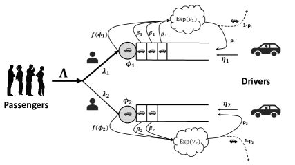
Figure 1: Depiction of system model

2.3 BCMP modeling of each platform

Under the aforementioned model, each platform can be described via a continuous time (Markovian) BCMP network [4]. Formally, the state of platform $i$ at time $t$ is given by the tuple $Z_{i,t}=(N_{i,t},R_{i,t})$, where $N_{i,t}$ is the number of waiting drivers, and $R_{i,t}$ is the number of drivers that are in the system but unavailable to be matched with passengers (because of being in a ride, or on a break). Realizations of the state of platform $i$ are represented as $({n_{i}},{r_{i}})$, and state space corresponding to platform $i$ is given by $S_{i}=\{({n_{i}},{r_{i}})\colon{n_{i}},{r_{i}}\in\mathbb{Z}_{+}\}$.

Each platform can be modelled using a BCMP network with two ‘service stations’ as described in the following: (i) service station 1 (SS1) is the queue of waiting drivers (the occupancy of this queue is the first dimension of the state), and (ii) service station 2 (SS2) is the ‘queue’ of drivers on a ride/break (the occupancy of this queue is the second dimension of the state). SS1 is modeled as a single server queue having a state-dependent service rate. Specifically, the (state dependent) departure rate from SS1 is $\lambda_{i}f(\phi_{i}(n_{i}))+{n_{i}}\beta_{i}.$ On the other hand, SS2 is modeled as an infinite server queue, having exponential service durations of rate $\nu_{i}.$ SS1 sees exogenous Poisson arrivals at rate $\eta_{i},$ and departures from SS1 become arrivals into SS2. Finally, departures from SS2 exit the system with probability $1-p_{i},$ and join SS1 with probability $p_{i};$ see Figure 1.

Next, we describe the steady state distribution corresponding to the above BCMP network (associated with platform $i$). Define $e_{i}:=\nicefrac{{\eta_{i}}}{{(1-p_{i})}},$ which is easily seen to be the effective driver arrival rate seen by the service stations SS1 and SS2. The following lemma follows from [4] (see Sections 3.2 and 5 therein).

Lemma 1.

The steady state probability of state $s=({n_{i}},{r_{i}})\in S_{i}$ is given by:

$$\pi_{i}(s) =C_{i}\left[\frac{{e_{i}}^{{n_{i}}}}{\prod_{a=1}^{{n_{i}}}\left(\lambda_{i}f(\phi_{i}(a))+a\beta_{i}\right)}\right]\left[\left({\frac{e_{i}}{\nu_{i}}}\right)^{{r_{i}}}\left(\frac{1}{{r_{i}}!}\right)\right],\text{ with }$$

$$C_{i}^{-1} =\sum_{n=0}^{\infty}\left[\frac{e_{i}^{n}}{\prod_{a=1}^{n}(\lambda_{i}f(\phi_{i}(a))+a\beta_{i})}\right]\exp\left({\frac{e_{i}}{\nu_{i}}}\right).$$

Here, $C_{i}$ is the normalizing constant (we follow the convention that $\prod_{a}^{k}(\cdot)=1$ when $a>k$).

2.4 Passenger split across platforms: Wardrop Equilibrium

We model the split of the aggregate passenger arrival rate $\Lambda$ into the system across the two platforms as a Wardrop equilibrium (WE) based on the Quality of Service (QoS); recall that platform $i$ sees passenger arrivals as per a Poisson process with rate $\lambda_{i}$. In particular, we consider two different QoS metrics in our analysis. However, before describing these formally, we first define the Wardrop split of the passenger arrival rate in terms of a generic QoS metric $Q.$

Let $Q_{i}(\lambda)$ denote the QoS of platform $i$ when the passengers arrive at rate $\lambda.$ Note that $Q_{i}$ will, in general, also depend on the pricing policy $\phi_{i}:=(\phi_{i}(n),\ n\in\mathbb{N})$ employed by platform $i,$ though this dependence is suppressed for simplicity. The Wardrop split $(\lambda_{1},\lambda_{2})$ under the price policy ${\bm{\phi}}=(\phi_{1},\phi_{2})$ is then defined as:

$${\lambda_{1}({{\bm{\phi}};\beta})}\in\underset{\lambda\in[0,\Lambda]}{\arg\min}\left(Q_{1}(\lambda)-Q_{2}(\Lambda-\lambda)\right)^{2},\quad{\lambda_{2}({{\bm{\phi}};\beta})}=\Lambda-{\lambda_{1}({{\bm{\phi}};\beta})}.$$ (2)

We address the uniqueness of the Wardrop split in Lemma 2 below. Having defined the Wardrop split in generic terms, we now define the passenger QoS metrics we consider. Note that passengers can leave the system without taking a ride either because of driver unavailability, or because of the price quoted was too high.

Let ${\cal U}_{i}$ be the long-run fraction of passengers who leave the system on account of driver unavailability. By the well-known PASTA property, this long run fraction equals the stationary probability of zero waiting drivers on platform $i$. Thus from Lemma 1,

$${\cal U}_{i}=\sum_{{r_{i}}=0}^{\infty}\pi_{i}((0,{r_{i}}))=\left(\sum_{n=0}^{\infty}\left[\frac{(e_{i})^{n}}{\prod_{a=1}^{n}(\lambda_{i}f(\phi_{i})+a\beta_{i})}\right]\right)^{-1}.$$ (3)

Let ${\cal B}_{i}$ be the long-run fraction of passengers that get blocked on platform $i,$ due to driver unavailability or a high price (this is the entire fraction that leave platform $i$ without taking a ride). Using PASTA again,

$${\cal B}_{i} ={\cal U}_{i}+\sum_{{n_{i}}=1}^{\infty}\sum_{{r_{i}}=0}^{\infty}(1-f(\phi_{i}({n_{i}})))\ \pi_{i}({n_{i}},{r_{i}}).$$ (4)

We use ${\cal U}_{i}~{}$ and ${\cal B}_{i}$ as our QoS metrics; note that these are both functions of $\lambda_{i}$. Our analysis for the case $Q_{i}={\cal U}_{i}$ (wherein the Wardrop split seeks to equalize the stationary probability of driver unavailability) is presented in Section 4, while the case $Q_{i}={\cal B}_{i}$ (wherein the Wardrop split seeks to equalize the stationary probability of passenger blocking) is addressed in Section 5. Next, we establish existence and uniqueness of the Wardrop equilibrium under these metrics (proof in Appendix Appendix A: Proofs of results stated in the main text); we first prove existence and uniqueness under a certain generic assumption (Assumption A.3 below), and then show that our metrics of interest satisfy the assumption.

1. The QoS function $Q_{i}$ for each  $i$ is continuous and strictly monotone in $\lambda_{i}$; both the functions are either increasing or decreasing.

Lemma 2.

Consider any QoS metric satisfying Assumption A.3. Given any price policy ${\bm{\phi}}=(\phi_{1},\phi_{2})$, there exists a unique Wardrop Equilibrium $({\lambda_{1}({{\bm{\phi}};\beta})},{\lambda_{2}({{\bm{\phi}};\beta})}).$

Finally, the QoS metrics $\{{\cal U}_{i}\}$ and $\{{\cal B}_{i}\}$ satisfy A.3 so long as $\beta_{i}>0$ for all $i.$

Given the existence and uniqueness of WE, we next define the platform utility functions. This defines a non-cooperative game between the two platforms.

2.5 Platform Utilities

We treat the action of each platform $i$ to be its pricing policy $\phi_{i}=(\phi_{i}(n),\ n\in\mathbb{N}).$ We define the utility of platform $i$ as the (almost sure) rate at which it derives revenue from matching drivers with passengers, denoted by ${\cal M}_{i}.$ Note that ${\cal M}_{i}$ depends on the price (action) profile ${\bm{\phi}}$ and other parameters; the pricing policy of each platform influences the other’s utility via the Wardrop split that determines the market shares of both platforms.

In the following, we derive the matching revenue rate (often referred to simply as the revenue rate) of each platform in terms of the Wardrop split $(\lambda_{1}({\bm{\phi}};\beta),\lambda_{2}({\bm{\phi}};\beta))$ (proof in Appendix Appendix A: Proofs of results stated in the main text).

Lemma 3.

The matching revenue rate of platform $i$ is given by,

$${\cal M}_{i}({\bm{\phi}},\lambda_{i}({\bm{\phi}};\beta);\beta)=\sum_{s_{i}\colon{n_{i}}\neq 0}\lambda_{i}({\bm{\phi}};\beta)f(\phi_{i}({n_{i}}))\phi_{i}({n_{i}})\pi_{i}(s_{i}).$$ (5)

2.6 Static prices and other simplifications

The goal of this paper is to analyse the game defined above between the two platforms. Since the analysis under dynamic pricing policies (where a platform’s price varies with the number of waiting drivers) is quite complex, we restrict attention to static pricing policies in this paper. Indeed, even the analysis under static pricing is non-trivial and highlights several novel insights. Note that under static pricing, the action space for each platform is simply $[0,\phi_{h}].$

Further, for simplicity of presentation, we consider symmetric platforms, i.e., we assume $e_{1}=e_{2}=e$ and $\beta_{1}=\beta_{2}=\beta.$ Accordingly, we study only symmetric equilibria in this study. As we will see, these equilibria will be parameterized by the driver-passenger ratio ($\mathsf{dpr}$), defined as $\rho:=\nicefrac{{e}}{{\Lambda}};$ note that the $\mathsf{dpr}$ captures the relative abundance of drivers and passengers in the system.

Finally, we approximate the utility functions of the platforms by letting $\beta\downarrow 0.$ This scaling regime, in which the patience times of waiting drivers are scaled to infinity, is referred to as the Infinite Driver Patience ($\mathsf{IDP}$) regime. While the $\mathsf{IDP}$ regime enables an explicit characterization of the equilibria of the non-cooperative game under consideration, it is also well motivated. Indeed, $\beta\approx 0$ means that driver abandonment times are stochastically much larger than ride durations and passenger interarrival times. This is reasonable in many practical scenarios, particularly when drivers are ‘tied’ to their respective platforms, and are available to take on rides for long durations (say an 8-10 hour work shift) at a stretch.

We conclude this section with a result characterizing the limit of the revenue rate of any platform as $\beta\to 0$ (proof in Appendix Appendix A: Proofs of results stated in the main text).

Lemma 4.

Suppose that for price policy ${\bm{\phi}}$, the passenger arrival rates $\lambda_{i}({\bm{\phi}};\beta)\to{\lambda}_{i}({\bm{\phi}};0)$ as $\beta\to 0$. Then the revenue rate (utility) of platform $i,$ ${\cal M}_{i}({\bm{\phi}},\lambda_{i}({\bm{\phi}};\beta);\beta),$ converges to ${\cal M}_{i}({\bm{\phi}},\lambda_{i}({\bm{\phi}};0);0)$ as $\beta\to 0,$ where

$${\cal M}_{i}({\bm{\phi}},\lambda_{i}({\bm{\phi}};0);0) =\begin{cases}{e}\phi_{i}&\text{ if }\left(\frac{{e}}{\lambda_{i}({\bm{\phi}};0)f(\phi_{i})}\right)<1,\\ \lambda_{i}({\bm{\phi}};0)f(\phi_{i})\phi_{i}&\text{ else.}\end{cases}$$ (6)

Along similar lines, we have ${\cal U}_{i}({\bm{\phi}},\lambda_{i}({\bm{\phi}},\beta);\beta)\to{\cal U}_{i}({\bm{\phi}},\lambda_{i}({\bm{\phi}};0),0)$, where

$${\cal U}_{i}({\bm{\phi}},\lambda_{i}({\bm{\phi}};0),0) =\max\left\{1-\frac{{e}}{\lambda_{i}({\bm{\phi}};0)f(\phi_{i})},0\right\}.$$ (7)

By virtue of the above result, we derive approximate equilibria of the actual system when $\beta$ is small, by analysing those in the $\mathsf{IDP}$ regime, which is obtained by letting $\beta\to 0.$ We also show that the equilibrium behavior in the $\mathsf{IDP}$ regime (which can be thought of as corresponding to $\beta=0$) is also meaningful in the more practical ‘pre-limit’ where $\beta$ is small and positive. Formally, we show that the equilibria under the $\mathsf{IDP}$ regime are $\epsilon$-equilibria when $\beta$ is small.

3 Monopoly

In this section, we consider a monopolistic scenario, where a single platform optimizes its pricing in the absence of competition. This analysis serves as a benchmark for the game theoretic analysis in the following sections (where the competition between platforms is captured explicitly), shedding light on the impact of inter-platform competition on pricing and passenger/platform utility.

Specifically, we analyse the pricing of a ‘monopolistic’ platform that sees a passenger arrival rate of $\nicefrac{{\Lambda}}{{2}},$ irrespective of its pricing strategy. (Other model details, including passenger price sensitivity and driver behavior, are as described in Section 2.) Note that this captures the behavior of each (symmetric) platform in our model from Section 2, if the passenger arrival rate seen by each platform is exogenously set to half the total arrival rate (as opposed to being set endogenously via the QoS based Wardrop split), to simulate the absence of competition.

In the monopolistic scenario, note that if the platform offers a price $\phi$ to an incoming passenger, then the passenger accepts this price with probability $f(\phi)$ (assuming a waiting driver is available). The revenue rate (utility) derived by the platform is then given by Lemma 3 with $\lambda=\nicefrac{{\Lambda}}{{2}}$ and the static policy $\phi(n)=\phi$ for all $n$ (see (5)):

$${\cal M}(\phi;\beta)=\frac{\Lambda}{2}f(\phi)\phi(1-{\cal U}(\phi;\beta)).$$ (8)

This revenue rate can be approximated using Lemma 4 when $\beta$ is close to zero. Formally, we define the utility of the platform in the $\mathsf{IDP}$ regime ($\beta=0$) as the pointwise limit of the utility as $\beta\to 0,$ i.e.,

$${\cal M}(\phi;0)=\begin{cases}e\phi&\text{ if }\phi<f^{-1}\left(2\rho\right),\\ \frac{\Lambda}{2}f(\phi)\phi&\text{ else.}\end{cases}$$ (9)

The optimal pricing strategy for the monopolistic platform that seeks to maximize ${\cal M}(\phi;0)$ is characterized as follows (proof in Appendix Appendix A: Proofs of results stated in the main text). (Recall that the driver-passenger ratio ($\mathsf{dpr}$) is defined as $\rho=\nicefrac{{e}}{{\Lambda}}.$)

Theorem 1.

Consider the $\mathsf{IDP}$ regime $(\beta=0)$. The optimal monopoly price is a non-increasing function of the $\mathsf{dpr}$ $\rho.$ Specifically, define

$${d_{m}}(\phi):=f(\phi)+\phi f^{\prime}(\phi),\ \phi_{m}:=\max\{\phi\in[0,\phi_{h}]:{d_{m}}(\phi)\geq 0\}.$$

1. If $\rho\leq f(\phi_{m})/2$, then $f^{-1}\left(2\rho\right)$ is the unique optimizer;

2. If $\rho>f(\phi_{m})/2$, then $\phi_{m}$ is the unique optimizer.

Moreover, for any sequence of optimal prices corresponding to a given sequence $\beta_{n}\to 0$, there exists a sub-sequence that converges to the unique optimal price of the $\mathsf{IDP}$ regime.

Theorem 1 presents a complete characterization of the optimal pricing policy for a monopolistic platform in the $\mathsf{IDP}$ regime, while also establishing the validity of this approximation when $\beta$ is positive and small, i.e., under the assumption of highly patient drivers. The optimal price is solely determined by the price sensitivity function $f$ and the $\mathsf{dpr}$ $\rho$. Indeed, the optimal price quoted by the platform decreases (formally non-increases) as a function of $\rho$, indicating that as the rate of driver arrivals increases (or equivalently, as the rate at which passengers enter the system decreases), the optimal price decreases, to induce a higher rate of matched rides. Formally, the optimal pricing may be interpreted as follows.

• It is instructive to first consider the special case ${d_{m}}(\phi_{h})\geq 0;$ this corresponds to the scenario where passengers are relatively price-insensitive. In this case, $\phi_{m}=\phi_{h}$ (as ${d_{m}}$ is decreasing), which also implies $f^{-1}(2\rho)=\phi_{h}$ (by definition) and hence $\phi_{h}$ is the unique optimizer under both parts (1)-(2). Thus it is optimal for the platform to exploit the passenger price-insensitivity and set the maximum permissible price $\phi_{h},$ irrespective of the $\mathsf{dpr}$.

• Next, consider the case ${d_{m}}(\phi_{h})<0$ and $\rho\leq f(\phi_{m})/2.$ This corresponds to the scenario where passengers are relatively price-sensitive, and the $\mathsf{dpr}$ is small (i.e., drivers are scarce relative to passengers). In this case, the optimal price equals $f^{-1}(2\rho),$ which is a decreasing function of $\mathsf{dpr}$, as expected—the scarcer the drivers, the higher the price.

• Finally, consider the case ${d_{m}}(\phi_{h})<0$ and $\rho>f(\phi_{m})/2.$ This corresponds to the scenario where passengers are relatively price-sensitive, and the $\mathsf{dpr}$ is large (i.e., passengers are scarce relative to drivers). This leads to a lower optimal price $\phi_{m},$ which does not vary further with the $\mathsf{dpr}$ $\rho$ (it is the maximizer of the function $f(\phi)\phi$); basically the system is saturated with an abundance of drivers, and $\nicefrac{{\Lambda}}{{2}}f(\phi)\phi$ represents the revenue rate of the system, which is maximized at $\phi_{m}$.

These observations are further corroborated by Figure 3 in Section 6.

In subsequent sections, we will draw insights by contrasting the monopolistic pricing strategy characterised here with the equilibrium strategy arising from the competition between the platforms. As noted before, this comparative analysis will shed light on how passenger-side churn affects the pricing policies of platforms.

4 Duopoly driven by driver unavailability

In this section, we analyse the competition between platforms, using driver unavailability as the QoS metric that governs the Wardrop split of the passenger arrival rate across platforms. Formally, in the language of Section 2, this corresponds to $Q_{i}={\cal U}_{i}$ given in (3) for all $i$. This defines a non-cooperative game between the platforms, wherein platforms use pricing as a lever to influence their market share (and payoffs). The goal of this section is to analyse and interpret the equilibria associated with this game. Our main insight is that when passengers are price-sensitive and scarce (relative to drivers), platforms are forced to deviate from monopoly pricing in order to ‘fight’ for market share, resulting in an equilibrium where both platforms are worse off (relative to the monopolistic scenario).

We begin by characterizing the unique Wardrop Equilibrium (WE) corresponding to any price (action) vector ${\bm{\phi}}=(\phi_{1},\phi_{2})$ in the following lemma (proof in Appendix Appendix A: Proofs of results stated in the main text).

Lemma 5.

For any $\beta>0$ and price vector ${\bm{\phi}}\in[0,\phi_{h}]^{2}$, the WE under QoS metric ${\cal U}$ is given by,

$$({\lambda_{1}({{\bm{\phi}};\beta})},{\lambda_{2}({{\bm{\phi}};\beta})})=\left(\frac{\Lambda f(\phi_{2})}{f(\phi_{1})+f(\phi_{2})},\frac{\Lambda f(\phi_{1})}{f(\phi_{1})+f(\phi_{2})}\right).$$

Importantly, note that Lemma 5 implies that the WE is insensitive to the value of $\beta$. This allows us to define the WE in the $\mathsf{IDP}$ regime ($\beta=0$) as

$$\lambda_{i}({\bm{\phi}};0)=\frac{\Lambda f(\phi_{-i})}{f(\phi_{i})+f(\phi_{-i})}.$$

Consequently, the payoff functions corresponding to the $\mathsf{IDP}$ regime, defined as the pointwise limits of the payoff functions as $\beta\downarrow 0,$ are given by:

$${\cal M}_{i}({\bm{\phi}};0)=\mathds{1}_{\{e<h({\bm{\phi}})\}}e\phi_{i}+\mathds{1}_{\{e\geq h({\bm{\phi}})\}}h({\bm{\phi}})\phi_{i},\text{ where }h({\bm{\phi}})=\lambda_{i}({\bm{\phi}};0)f(\phi_{i}).$$ (10)

The above expression follows easily from Lemma 4. We now characterize the (symmetric) equilibria corresponding to the $\mathsf{IDP}$ regime (i.e., the non-cooperative game defined by the payoff functions (10)).

4.1 Equilibria in the $\mathsf{IDP}$ regime

The following theorem provides a complete characterization of the symmetric Nash equilibria (NE) in the $\mathsf{IDP}$ regime (proof in Appendix Appendix A: Proofs of results stated in the main text).

Theorem 2.

Consider the $\mathsf{IDP}$ regime $(\beta=0)$. Define

$${d_{u}}(\phi):=2f(\phi)+\phi f^{\prime}(\phi),\ \phi_{u}:=\max\{\phi\in[0,\phi_{h}]:{d_{u}}(\phi)\geq 0\}.$$

1. If $\rho\leq f(\phi_{u})/2$, then $\left(f^{-1}\left(2\rho\right),f^{-1}\left(2\rho\right)\right)$ is the unique symmetric NE;

2. If $\rho>f(\phi_{u})/2$, then $(\phi_{u},\phi_{u})$ is the unique symmetric NE.

Theorem 2 provides insights on how competition between platforms influences their pricing. Importantly, the equilibrium price quoted by each platform is a decreasing (formally, non-increasing) function of the $\mathsf{dpr}$ $\rho$. This means that as the rate of driver arrivals increases (or equivalently, as the rate at which passengers enter the system decreases), the competition between platforms for market share intensifies, resulting in a lower equilibrium price.

Next, we formally interpret the equilibrium prices established in Theorem 2. It must be emphasized that while there are clear structural similarities between the statements of Theorem 2 and Theorem 1 (which addresses the optimal monopoly pricing), the quantities ${d_{m}}$ and $\phi_{m}$ in the former differ from the corresponding quantities ${d_{u}}$ and $\phi_{u}$ in the latter. Indeed, it is easy to see that ${d_{u}}(\cdot)>{d_{m}}(\cdot),$ and $\phi_{u}\geq\phi_{m}.$

• As before, we first consider the special case ${d_{m}}(\phi_{h})\geq 0;$ this corresponds the scenario where passengers are relatively price-insensitive. In this case, $\phi_{u}=f^{-1}(2\rho)=\phi_{h}$, indicating as before that the unique NE corresponds to both platforms charging the maximum permissible price, which is also the optimal monopoly price. In other words, inter-platform competition becomes inconsequential when customers are this insensitive to price; each platform can maximize its profit by charging the highest possible price, regardless of the $\mathsf{dpr}$.

• Next, consider the case ${d_{m}}(\phi_{h})<0$ & $\rho\leq f(\phi_{u})/2;$ this corresponds to the scenario where passengers are relatively price sensitive, and the $\mathsf{dpr}$ is small (i.e., drivers are scarce relative to passengers). In this case, it also holds that $\rho\leq f(\phi_{m})/2;$ this means the equilibrium price coincides with the optimal monopoly price, which is equal to $f^{-1}(2\rho)$. In other words, when passengers are price-sensitive, but abundant (relative to drivers), inter-platform competition becomes inconsequential and both platforms operate on monopoly pricing.

• Finally, consider the case ${d_{m}}(\phi_{h})<0$ & $\rho>f(\phi_{u})/2;$ this corresponds to the scenario where passengers are relatively price sensitive, and the $\mathsf{dpr}$ is large (i.e., passengers are scarce relative to drivers). In this case, the platforms are forced to compete for market share, and the equilibrium pricing deviates from the optimal monopoly pricing. In other words, when passengers are price sensitive and scarce, competition drives each platform to a sub-optimal price. In particular, as we show in Lemma 7 (see Section 6), the equilibrium price in this case is strictly greater than the monopoly price. Intuitively, this is because platforms try to boost the QoS driver availability (and therefore market share) by raising prices (even at the expense of losing some passengers).

In Section 6, we conduct a comprehensive comparison of the equilibrium prices derived from Theorem 2 and the optimal monopolistic price as characterized in Section 2. This analysis also sheds light on the welfare implications of platform competition in different market conditions.

4.2 Applicability of $\mathsf{IDP}$ equilibria in the pre-limit (i.e., for small $\beta>0$)

We now establish a connection between the NE in the $\mathsf{IDP}$ regime (Theorem 2) and equilibrium behavior in the system when $\beta$ is positive and small. Specifically, we show that the NE in the $\mathsf{IDP}$ regime is an $\epsilon$-NE in the pre-limit. We recall here the definition of an $\epsilon$-NE (see [20, Section 3.13]).

Definition 1 ($\epsilon$-NE).

Consider a strategic form game $G=\left<\mathcal{N},(\Phi_{i}),({\cal M}_{i})\right>$ where $\mathcal{N}$ is a finite set, the $\Phi_{i}$ are nonempty compact metric spaces, and the ${\cal M}_{i}:\Phi_{i}\to\mathbb{R}$ are utility functions. Given $\epsilon\geq 0,$ a mixed strategy $\sigma$ is called an $\epsilon$-NE if for all $i\in\mathcal{N}$ and $\phi_{i}\in\Phi_{i}$,

$${\cal M}_{i}(\phi_{i},\sigma_{-i})\leq{\cal M}_{i}(\sigma_{i},\sigma_{-i})+\epsilon.$$

Note that when $\epsilon=0$, an $\epsilon$-NE is just an NE in the usual sense.

The notion of $\epsilon$-NE relaxes the notion of the NE in that no player stands to make a utility gain exceeding $\epsilon$ from a unilateral deviation.

Theorem 3.

Consider any $\epsilon>0$. There exists ${\bar{\beta}}_{\epsilon}>0$ such that for $0<\beta\leq{\bar{\beta}}_{\epsilon}$, the unique symmetric NE $(\phi^{*},\phi^{*})~{}$ of the $\mathsf{IDP}$ regime (as characterized in Theorem 2) is an $\epsilon$-NE.

Theorem 3 (proof in Appendix Appendix A: Proofs of results stated in the main text) essentially validates Theorem 2, by showing that the equilibria in the $\mathsf{IDP}$ regime are also meaningful in the pre-limit (i.e., when $\beta$ is small and positive). In other words, under the assumption of fairly patient drivers, our analysis of the $\mathsf{IDP}$ regime is indicative of equilibrium behavior of the platforms, and the conclusions of Theorem 2 are applicable.

5 Duopoly driven by price & driver unavailability

In this section, we analyse the competition between platforms under a different passenger QoS metric, that captures the overall likelihood of finding a ride on arrival (note that a ride may not materialise either due to driver unavailability, or because the price is unacceptable). Formally, in the language of Section 2, this corresponds to $Q_{i}={\cal B}_{i}$ for all $i.$ The goal of this section is to analyse and interpret the equilibria associated with the corresponding non-cooperative game between the platforms. Our main insight is that when passengers are scarce (relative to drivers), platforms are forced to deviate from monopoly pricing in order to ‘fight’ for market share. Moreover, we find that the nature of this deviation is quite different from what was observed in Section 4 (where the WE split was assumed to be governed by driver unavailability alone). In particular, we find that under certain conditions, no pure NE exists; instead, we demonstrate a mixed NE, and also a novel equilibrium concept having dynamic connotations, that we call an equilibrium cycle.

We begin by defining the $\mathsf{IDP}$ regime formally. Recall that the payoff functions in the $\mathsf{IDP}$ regime are pointwise limits of our payoff functions as $\beta\to 0.$ Note that the passenger blocking probability on platform $i$ when it uses static price policy $\phi_{i}$ and when passengers arrive at rate $\lambda_{i}$ is given by (see (4)),

$${\cal B}_{i}({\bm{\phi}};\beta) ={\cal U}_{i}({\bm{\phi}};\beta)+(1-f(\phi_{i}))(1-{\cal U}_{i}({\bm{\phi}};\beta))={\cal U}_{i}({\bm{\phi}};\beta)f(\phi_{i})+(1-f(\phi_{i})),$$ (11)

the limiting value of which, as $\beta\to 0,$ is given by (using Lemma 4)

$${\cal B}_{i}({\bm{\phi}};\lambda_{i}({\bm{\phi}},0))=\begin{cases}1-\frac{{e}}{\lambda_{i}}&\text{ if }\left(\frac{{e}}{\lambda_{i}f(\phi_{i})}\right)<1,\\ 1-f(\phi_{i})&\text{ else.}\end{cases}$$ (12)

As before, the revenue rate of platform $i$, when the two platforms operate with the static price vector ${\bm{\phi}},$ equals ${\cal M}_{i}({\bm{\phi}})={\cal M}_{i}({\bm{\phi}};{\lambda_{i}({{\bm{\phi}};\beta})})$, where the WE splits ${\lambda_{i}({{\bm{\phi}};\beta})}$ are defined using the QoS metric ${\cal B}$. In the following, we first characterize the limiting WE as $\beta\to 0,$ and subsequently the limiting payoff functions.

Theorem 4.

Fix price vector ${\bm{\phi}}$. Extend the definition of WE and revenue rate ${\cal M}$ as in Table 1. Then for any $i\in\{1,2\}$, the two mappings $\beta\mapsto\lambda_{i}({\bm{\phi}};\beta)$ and $\beta\mapsto{\cal M}_{i}({\bm{\phi}};\beta)$ are continuous over $[0,\infty)$.

	Range of $\phi_{1}$ when $\phi_{1}>\phi_{2}$			Range of $\phi_{1}$ when $\phi_{1}=\phi_{2}$
	$[0,f^{-1}(2\rho))$	$[f^{-1}(2\rho),f^{-1}(\rho))$	$[f^{-1}(\rho),\phi_{h}]$	$[0,f^{-1}(2\rho))$	$[f^{-1}(2\rho),\phi_{h}]$
$\lambda_{1}({\bm{\phi}};0)$	$\nicefrac{{\Lambda}}{{2}}$	$\Lambda-\nicefrac{{e}}{{f(\phi_{1})}}$	0	$\nicefrac{{\Lambda}}{{2}}$	$\nicefrac{{\Lambda}}{{2}}$
${\cal M}_{1}({\bm{\phi}};0)$	$e\phi_{1}$	$m(\phi_{1})$	0	$e\phi_{1}$	$\nicefrac{{\Lambda}}{{2}}f(\phi_{1})\phi_{1}$
${\cal M}_{2}({\bm{\phi}};0)$	$e\phi_{2}$	$e\phi_{2}$	$\Lambda f(\phi_{2})\phi_{2}$	$e\phi_{2}$	$\nicefrac{{\Lambda}}{{2}}f(\phi_{2})\phi_{2}$

Table 1: $\mathsf{IDP}$ regime under QoS ${\cal B}$. Here, $m(\phi)=(\Lambda f(\phi)-{e})\phi$, $\lambda_{2}({\bm{\phi}};0)=\Lambda-\lambda_{1}({\bm{\phi}};0).$ When $\phi_{1}<\phi_{2},$ reverse the role of $\phi_{1},$ and $\phi_{2}.$

In essence, Theorem 4 (proof in Appendix Appendix A: Proofs of results stated in the main text) defines the $\mathsf{IDP}$ regime ($\beta=0$), by specifying the payoff of each player as a function of the price (action) profile. In the remainder of this section, we analyse the equilibria in the $\mathsf{IDP}$ regime, and then show that these are also meaningful in the ‘pre-limit’ (i.e., when $\beta$ is small).

5.1 Equilibria in the $\mathsf{IDP}$ regime

The following theorem characterizes the Nash equilibria of the $\mathsf{IDP}$ regime (proof in Appendix Appendix A: Proofs of results stated in the main text).

Theorem 5.

Consider the $\mathsf{IDP}$ regime $(\beta=0)$. Define

$${d_{b}}(\phi):=f(\phi)+2\phi f^{\prime}(\phi),\ \phi_{b}=\max\{\phi\in[0,\phi_{h}]:{d_{b}}(\phi)\geq 0\}.$$

1. If $\rho\leq f(\phi_{b})/2,$ then $\left(f^{-1}\left(2\rho\right),f^{-1}\left(2\rho\right)\right)~{}$ is the unique symmetric NE;

2. If $f(\phi_{b})/2<\rho<1,$ then there does not exist a symmetric pure strategy NE. However, there exists a symmetric mixed strategy NE  $(\sigma^{*},\sigma^{*}),$ supported over $[{\phi_{L}^{*}},{\phi_{R}^{*}}]$, where ${\phi_{L}^{*}},{\phi_{R}^{*}}$ are respectively the maximum value and the maximizer of the function $\phi\mapsto(f(\phi)-\rho)\phi/\rho$, and

   $$\sigma^{*}([{\phi_{L}^{*}},\phi])=\frac{e(\phi+{\phi_{R}^{*}})-\Lambda f({\phi_{R}^{*}}){\phi_{R}^{*}}}{2e\phi-\Lambda f(\phi)\phi}\text{ for }\phi\in[{\phi_{L}^{*}},{\phi_{R}^{*}}];$$

3. If $\rho\geq 1$ then for any $\epsilon>0$, choose $0<\delta\leq\phi_{h}~{}$ such that  $\sup_{\phi\leq\delta}\Lambda f(\phi)\phi<\epsilon$. Then $(\delta,\delta)$ is an $\epsilon$-NE.

Theorem 5 characterizes the impact of competition between platforms on their equilibrium pricing strategies (with market shares determined by the QoS metric ${\cal B}_{i}$). Crucially, the nature of the equilibrium itself depends on the $\mathsf{dpr}$, which captures the relative abundance of drivers and passengers—a pure strategy NE arises over a certain range, a mixed strategy NE arises over another, and finally, an $\epsilon$-NE arises the $\mathsf{dpr}$ exceeds 1. Similar to previous sections, the equilibrium price tends to decrease as a function of the $\mathsf{dpr}$ $\rho$. In other words, as the rate of driver arrivals increases (or conversely, as the rate at which passengers enter the system decreases), the competition between platforms intensifies, resulting in a lower equilibrium price.

Next, we formally interpret the equilibrium prices as established in Theorem 5. Once again, it is important to emphasize that although there are clear structural similarities between the statements of Theorems 1, 2, and 5, the quantities ${d_{b}}$ and $\phi_{b}$ in the latter differ from their counterparts in the previous theorems.

• We begin by considering the case $\rho\leq f(\phi_{m})/2;$ this corresponds to the scenario where drivers are scarce relative to passengers. Under these favourable market conditions, the equilibrium is characterized by both platforms operating at the optimal monopoly price $f^{-1}\left(2\rho\right)$.

• Next, consider the case $f(\phi_{m})/2<\rho\leq f(\phi_{b})/2;$ this corresponds to the scenario where the $\mathsf{dpr}$ $\rho$ is somewhat larger (i.e., drivers are less scarce relative to passengers). In this case, competition between the platforms induces a deviation from the optimal monopoly price; each platform sets an equilibrium price $f^{-1}\left(2\rho\right)$ that is strictly smaller than the optimal monopoly price $\phi_{m}$.

• Next, consider the case $f(\phi_{b})/2<\rho<1;$ this corresponds to the scenario where the $\mathsf{dpr}$ $\rho$ is quite large, indicating a scarcity of passengers (relative to drivers). In this case, competition between the platforms intensifies, leading to a further deviation of the equilibrium behavior from the monopoly setting. In particular, a pure strategy NE does not even exist in this case. Formally, this is because of certain discontinuities in the payoff functions, which are in turn induced by discontinuities in the Wardrop split. Indeed, when passengers are scarce, the Wardrop split is primarily dictated by price; as a consequence, a slight reduction in price by one platform (below the price posted by the other) can result in a significant jump in its market share. Figure 2 provides an illustration of this payoff function discontinuity in the $\mathsf{IDP}$ regime.

  While a pure NE does not exist if $f(\phi_{b})/2<\rho<1$ owing to the above mentioned payoff discontinuities, we show that there does exist a symmetric mixed NE in this case, characterized by a continuous distribution $\sigma^{*}$ supported over the closed interval $[{\phi_{L}^{*}},{\phi_{R}^{*}}]$. We note that both ${\phi_{L}^{*}}$ and ${\phi_{R}^{*}}$ are decreasing (formally, non-increasing) functions of $\rho$. While the mixed NE allows one to interpret the equilibrium behavior of the platforms via randomised prices, a dynamic interpretation in terms of oscillating prices is also possible. We formalise this interpretation below by introducing a novel equilibrium called equilibrium cycle (EC), and show that in this case, $[{\phi_{L}^{*}},{\phi_{R}^{*}}]$ is also an EC.

• Finally, consider the case $\rho\geq 1;$ this corresponds to the scenario where passengers are very scarce, driving both platforms to operate at near zero prices. Formally however, it can be shown that $(0,0)$ is not a NE. Instead, we show that $(\delta,\delta)$ is an $\epsilon$-NE for suitably small values of $\delta$ and $\epsilon$, suggesting that players choose a price ‘close to zero’ in such a competitive environment.

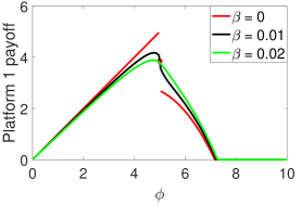
Figure 2: Depiction of discontinuity of ${\cal M}_{1}(\phi,\phi_{2})$ v/s $\phi$ (fixing $\phi_{2}=5)$ in the $\mathsf{IDP}$ regime, with $\Lambda=2,e=1,\phi_{h}=10,f(\phi)=1-(a\phi)^{2}$, where $a=0.1$.

We now revisit the case $f(\phi_{b})/2<\rho<1,$ with the aim of developing a dynamic interpretation of the strategic interaction between platforms. It is instructive to consider the incentives for unilateral deviation in price by each platform in this case. Specifically, it turns out that when the opponent, say platform $-i,$ offers a price within the interval $[{\phi_{L}^{*}},{\phi_{R}^{*}}],$ platform $i$ is incentivised to also set its price within the same interval. In particular, if the opponent’s price lies within the range $({\phi_{L}^{*}},{\phi_{R}^{*}}],$ platform $i$ has an incentive (though not a best response, which does not exist) to set its price slightly below the opponent. On the other hand, if the opponent’s price is ${\phi_{L}^{*}},$ then platform $i$’s best response is to set its price at ${\phi_{R}^{*}}.$ In essence, this suggests an indefinite oscillation of prices within the interval $[{\phi_{L}^{*}},{\phi_{R}^{*}}].$ This motivates the following notion of an equilibrium cycle.

Definition 2 (Equilibrium Cycle).

A closed interval $[a,b]$ is called an equilibrium cycle (EC) if:

1. for any $i\in\mathcal{N}$, for $\phi_{-i}\in[a,b],$ there exists $\phi_{i}\in[a,b]$ such that,

   $$\mathcal{M}_{i}(\phi_{i},\phi_{-i})>\mathcal{M}_{i}(\tilde{\phi}_{i},\phi_{-i})\ \forall\ \tilde{\phi}_{i}\in[0,\phi_{h}]\setminus[a,b],$$

2. for any price vector ${\bm{\phi}}\in[a,b]^{2}$, there exists $i\in\mathcal{N}$ and $\phi_{i}^{\prime}\in[a,b]$ such that ${\cal M}_{i}(\phi_{i}^{\prime},\phi_{-i})>{\cal M}_{i}({\bm{\phi}})$ and

   $$\mathcal{M}_{i}(\phi_{i}^{\prime},\phi_{-i})>\mathcal{M}_{i}(\tilde{\phi}_{i},\phi_{-i})\ \forall\ \tilde{\phi}_{i}\in[0,\phi_{h}]\setminus[a,b],$$

3. no subset of $[a,b]$ satisfies the above two conditions.

The first condition above establishes the ‘stability’ of the interval $[a,b];$ if any player plays an action in this interval, the other player is also incentivized to play an action in the same interval (this choice dominating any action outside the interval). The second condition establishes the ‘cyclicity’ of the same interval; if both players play any actions within the interval $[a,b]$, at least one player has the incentive to deviate to a different action within the same interval (this deviation also dominating any action outside the interval). The last condition ensures the minimality of the interval, i.e., no strict subset of an EC is an EC.

Theorem 6.

Consider the $\mathsf{IDP}$ regime $(\beta=0)$. If $f(\phi_{b})/2<\rho<1,$ then the interval $[{\phi_{L}^{*}},{\phi_{R}^{*}}]$ is an equilibrium cycle.

Theorem 6 establishes that if $f(\phi_{b})/2<\rho<1,$ the support of the symmetric mixed NE as established in Theorem 5 is also an equilibrium cycle. Intuitively, this EC can be interpreted (in dynamic terms) as the limit set of alternating ‘better’ response dynamics between the platforms (not that best response may not exist in this case owing to the payoff function discontinuities discussed before). We provide numerical illustrations of these oscillating dynamics in Figure 6.

Finally, we comment of the payoff of each platform in this case.

Lemma 6.

If $f(\phi_{b})/2<\rho<1,$ then the average payoff of each platform $i$ under the mixed NE $(\sigma^{*},\sigma^{*})$ is given by ${\cal M}_{i}(\sigma^{*},\sigma^{*};0)=m({\phi_{R}^{*}}).$ Moreover, the security value and strategy of each platform are $m({\phi_{R}^{*}})$ and ${\phi_{R}^{*}},$ respectively.

Interestingly, the average payoff of each platform under the mixed ME agrees with its security value. Moreover, this is also the payoff that each platform receives when one platform plays the price ${\phi_{L}^{*}}$ (the left endpoint of the EC) and the other plays the price ${\phi_{R}^{*}}$ (the right endpoint of the EC), which is its best response to the opponent’s action, and also the security strategy.

5.2 Applicability of $\mathsf{IDP}$ regime equilibria in the pre-limit (for small $\beta>0$)

We now establish a connection between the equilibria in the $\mathsf{IDP}$ regime (Theorems 5 and 6) and equilibrium behavior in the pre-limit, where $\beta$ is small and positive. Specifically, as was also done in Section 4, we show that the equilibria of the $\mathsf{IDP}$ regime are $\epsilon$-equilibria in the pre-limit. Towards this, we begin by defining an $\epsilon$-EC.

Definition 3 ($\epsilon$-equilibrium cycle).

A closed interval $[a,b]$ is called an $\epsilon$-equilibrium cycle ($\epsilon$-EC) if:

1. for any $i\in\mathcal{N}$, for $\phi_{-i}\in[a+\epsilon,b-\epsilon],$ there exists $\phi_{i}\in[a,b]$ such that,

   $$\mathcal{M}_{i}(\phi_{i},\phi_{-i})>\mathcal{M}_{i}(\tilde{\phi}_{i},\phi_{-i})\ \forall\ \tilde{\phi}_{i}\in[0,\phi_{h}]\setminus[a-\epsilon,b+\epsilon],$$

2. for any price vector ${\bm{\phi}}\in[a+\epsilon,b-\epsilon]^{2}$, there exists $i\in\mathcal{N}$ and $\phi_{i}^{\prime}\in[a,b]$ such that  ${\cal M}_{i}(\phi_{i}^{\prime},\phi_{-i})>{\cal M}_{i}({\bm{\phi}})~{}$ and

   $$\mathcal{M}_{i}(\phi_{i}^{\prime},\phi_{-i})>\mathcal{M}_{i}(\tilde{\phi}_{i},\phi_{-i})\ \forall\ \tilde{\phi}_{i}\in[0,\phi_{h}]\setminus[a-\epsilon,b+\epsilon],$$

3. there exists no subset $[c,d]$ of $[a+\epsilon,b-\epsilon]$ that satisfies conditions  $(i)-(ii)$.

The definition of an $\epsilon$-EC relaxes the notion of the EC, permitting platforms to deviate from EC strategies by a margin of $\epsilon$. This relaxation preserves the key properties of the EC while allowing for small deviations in the space of actions.

Theorem 7.

Consider $\rho<1$. Then for any $\epsilon>0$, there exists ${\bar{\beta}}_{\epsilon}>0$ such that for all $0<\beta\leq{\bar{\beta}}_{\epsilon}$,

1. the NE defined in Theorem 5 for the $\mathsf{IDP}$ regime (both pure and mixed) are $\epsilon$-NE, and

2. if $f(\phi_{b})/2<\rho<1,$ then the interval $[{\phi_{L}^{*}},{\phi_{R}^{*}}]$ defined in Theorem 6 is an $\epsilon$-EC.

As before, Theorem 7 validates Theorems 5 and 6 by showing that the equilibria in the $\mathsf{IDP}$ regime are also meaningful in the pre-limit (i.e., when $\beta$ is small and positive). In other words, under the practical assumption that drivers are patient, our characterization of the $\mathsf{IDP}$ regime equilibria are indicative of equilibrium behavior of the platforms.

6 Comparisons and numerical results

In this section, we compare the equilibria characterized in the previous sections (under different assumptions on how the passenger arrival rate gets split between platforms), both analytically as well as via numerical experiments. We also demonstrate how our results for the $\mathsf{IDP}$ regime ($\beta=0$) are applicable in the pre-limit.

6.1 Comparisons

The following lemma compares the monopoly optimum prices derived in Section 3 and the equilibrium prices derived in Sections 4 and 5.

Lemma 7.

Consider the $\mathsf{IDP}$ regime ($\beta=0$).

1. The equilibrium price under QoS metric ${\cal U}$ is greater than or equal to the optimal monopoly price.

2. The equilibrium price under QoS metric ${\cal B}$ is less than or equal to the optimal monopoly price.

Moreover, the optimal platform payoff in the monopolistic scenario is always greater than or equal to the equilibrium payoff (under either of our models for inter-platform competition). In this comparison, we treat the equilibrium price and platform payoff under QoS metric ${\cal B}$ to be zero for $\rho\geq 1,$ in line with Statement (3) of Theorem 5.

Lemma 7 (proof in Appendix Appendix A: Proofs of results stated in the main text) provides valuable insights into the interplay between competition, QoS and platform utility. In particular, we find that competition drives platforms to set prices that deviate from the optimal monopoly price, so as to enhance that very QoS metric that governs the market share split. Indeed, when the market split is governed by QoS metric ${\cal U},$ the equilibrium price exceeds the monopoly price, since driver availability is boosted by higher prices. On the other hand, when the market split is governed by QoS metric ${\cal B},$ equilibrium prices are lower than the monopoly price, given that stationary probability that an arriving passenger obtains a ride gets boosted by a price reduction. In either case, we see that inter-platform competition enhances QoS on the passenger side, while diminishing the equilibrium payoff of each platform.

Next, we numerically evaluate and compare the optimal/equilibrium prices and corresponding platform utilities across the monopoly and competition models. We consider a non-linear price sensitivity function, $f(\phi)=1-(a\phi)^{2}$ for some $a<1/\phi_{h}$ (this choice satisfies Assumptions A.1-2). By performing simple algebraic calculations, we compute the following quantities defined in Theorems 1–7, which characterize the different equilibria.

$\phi_{m}=\frac{1}{\sqrt{3}a}$,	$\phi_{b}=\frac{1}{\sqrt{5}a}$,	$f^{-1}(2\rho)=\left(\frac{1}{a}\right)\sqrt{1-2\rho}$,
$\phi_{u}=\frac{1}{\sqrt{2}a}$,	${\phi_{L}^{*}}=\left(\frac{2}{3a}\right)\left(\frac{1}{\rho}-1\right)\sqrt{\frac{1-\rho}{3}}$,	${\phi_{R}^{*}}=\left(\frac{1}{a}\right)\sqrt{\frac{1-\rho}{3}}$.

In Figure 3, we plot the optimal/equilibrium price (left panel) and platform utility (right panel) as a function of the $\mathsf{dpr}$ $\rho$ (specifically, we hold $\Lambda$ fixed and vary $e$). For the case where market share is governed by QoS metric ${\cal B},$ the support of the mixed NE (or the EC) is marked via vertical black lines in the left panel; in the right panel, we plot the average payoff corresponding to the mixed NE (or equivalently, the security value; see Lemma 6). Note that the pricing is in line with the conclusions of Sections 3–5 and Lemma 7. It is instructive to note the variation of the optimal/equilibrium platform utility as $\rho$ increases (specifically, as $e$ increases with $\Lambda$ being fixed):

• Platform utility first increases and then saturates, in the monopoly setting, as well as in the setting where market share is governed by QoS metric ${\cal U}.$ This is because as driver availability grows, platforms are able to match more passengers with rides, until driver availability is no longer a constraint.

• In contrast, in the setting where market share is governed by QoS metric ${\cal B},$ platform utility first increases and then decreases, approaching zero as $\rho$ approaches 1. This is because competition drives the equilibrium price close to zero as $\rho$ approaches 1.

• Under both competition models, the price of anarchy (from the standpoint of the platforms) exceeds one when $\rho$ is large, i.e., when passengers are scarce relative to drivers.

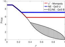
(a) Equilibrium/optimal price versus $\rho$

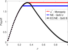
(b) Equilibrium/optimal platform payoff versus $\rho$

Figure 3: Price sensitivity function $f(\phi)=1-(a\phi)^{2},$ where $a=0.1$ and $\phi_{h}=9,$ $\Lambda=1.$

6.2 Cooperation versus competition

We now study an alternate cooperative scenario in which the platforms operate together, by pooling their driver resources to jointly serve the entire passenger demand. Mathematically, the analysis of this scenario is identical to that corresponding to the monopoly scenario (see Section 3), but with passenger arrival rate $\nicefrac{{\Lambda}}{{2}}$ being replaced by $\Lambda,$ and effective driver arrival $e$ being replaced by $2e.$

Since the $\mathsf{dpr}$ $\rho$ remains unchanged under the above scaling, the optimal pricing in the $\mathsf{IDP}$ regime ($\beta=0)$ for this cooperative setting is exactly as stated in Theorem 1. This also means that the payoff of each platform (assuming an equitable revenue split) is also identical to that in the monopoly setting. In light of Lemma 7, we conclude that cooperation is beneficial to the platforms (while being detrimental to the passenger base).

Interestingly, the above observation suggests that in the $\mathsf{IDP}$ regime (and via continuity, also when $\beta$ is small, i.e., assuming drivers are patient), the economies of scale one typically expects from resource pooling in queueing systems do not arise. However, when $\beta$ is large, i.e., drivers are relatively impatient, we find that the platforms do indeed benefit from the economies of scale resulting from resource pooling—see Figure 4, which compares the optimal price and (per-platform) payoff in the monopoly setting (where each platform sees an exogenous passenger arrival rate of $\nicefrac{{\Lambda}}{{2}}$) and the cooperative setting (where both platforms jointly serve passengers at rate $\Lambda$). Note that the per-platform payoff is higher in the cooperative setting (and this is achieved by operating at a lower price) compared to the monopoly setting when $\beta$ is large. Given our previous observation that competition results in an equilibrium payoff less than the monopoly payoff, this suggests that cooperation is even more beneficial to the platforms if drivers are impatient.

(a) Optimal price versus $\beta$

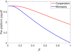
(b) Per-platform payoff versus $\beta$

Figure 4: Comparison between cooperative setting and monopoly setting; here, $e=2$, $\Lambda=3$, $\phi_{h}=10,$ $f(\phi)=1-(a\phi)^{2}$, with $a=\nicefrac{{1}}{{10.01}}$

6.3 Numerical demonstrations of the connection between $\mathsf{IDP}$ regime equilibria and pre-limit equilibria

We now provide some numerical evidence to complement the conclusions of Theorems 3 and 7, which show that the equilibria characterized for the $\mathsf{IDP}$ regime $(\beta=0)$ are also meaningful when $\beta$ is small (i.e., drivers are relatively patient).

We begin by considering the case of competition under the QoS metric ${\cal U}.$ In Figure 5, we plot the actions (prices) corresponding to alternating best response (BR) dynamics between the platforms for different choices of $\beta.$ For reference, the figure also shows the NE corresponding to the $\mathsf{IDP}$ regime as characterized in Theorem 2. There are two key takeaways from this figure:

• Alternating BR dynamics appear to converge when $\beta$ is small and positive. This suggests the existence of a pure NE even in the pre-limit.

• The above limit is close to the NE corresponding to the $\mathsf{IDP}$ regime. This in turn suggests that the NE in the pre-limit is ‘close’ to the NE in the $\mathsf{IDP}$ regime.

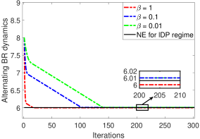
Figure 5: Alternating best response dynamics; $e=1,\Lambda=5,\phi_{h}=10,f(\phi)=1-(a\phi)^{2}$ with $a=\nicefrac{{1}}{{10.01}}$.

Next, we consider the case of competition under the QoS metric ${\cal B}.$ In Figure 6, we plot the actions (prices) corresponding to alternating best response (BR) dynamics between the platforms for different choices of $\beta,$ for a choice of system parameters that induces an equilibrium cycle in the $\mathsf{IDP}$ regime. (Note that even through best responses do not exist in the $\mathsf{IDP}$ regime, they do exist in the pre-limit.) Interestingly, we find that the best response dynamics oscillate in the pre-limit; moreover, the support of this oscillation aligns closely with the equilibrium cycle in the $\mathsf{IDP}$ regime as characterized in Theorem 6 (the $\mathsf{IDP}$ regime EC is depicted using dotted red lines in Figure 6). These observations are consistent with our dynamic interpretation of the equilibrium cycle in Section 5.

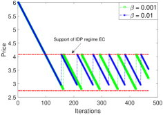
(a) Dynamics initialized above the $\mathsf{IDP}$ regime EC

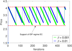
(b) Dynamics initialized below the $\mathsf{IDP}$ regime EC

Figure 6: Alternating BR dynamics starting from two different points outside the $\mathsf{IDP}$ regime EC; $e=1$, $\Lambda=2$, $f(\phi)=1-(a\phi)^{2}$ with $a=\nicefrac{{1}}{{10.01}}$.

7 Concluding Remarks

We consider competing ride-hailing platforms with impatient, price-sensitive passengers and impatient and revisiting drivers. On the one hand, each platform strives to meet its passengers’ QoS goals so as to capture a larger market share (the total market share across platforms is conserved). On the other hand, they also seek to increase their prices so as to maximize their long-run revenue rate. Our analysis thus sheds light on the intricate interplay between competition, price-sensitivity, and the relative scarcity/surplus of drivers relative to passengers.

A key feature of our analysis is that we provide closed form characterizations of the equilibrium prices in a certain limiting regime, which we refer to as the infinite driver patience regime. Interestingly, we find that the equilibrium prices depend on (i) the price sensitivity of the passenger base, and (ii) the ratio of driver and passenger arrival rates. This latter quantity appears to play a role analogous to the utilization/load in classical queueing models. In particular, we find that competition drives platforms to set prices that deviate from the ‘optimal’ values when passengers are price-sensitive and scarce (relative to drivers); moreover, the deviation seeks to enhance the QoS experienced by the passenger base.

From a game theoretic standpoint, our analysis also demonstrates some interesting equilibrium behavior. Specifically, in certain cases, we find that discontinuities in payoff functions can result in there being no pure Nash equilibrium. Instead, we demonstrate a mixed equilibrium, as well as a novel equilibrium concept with interesting dynamic connotations that we refer to as an equilibrium cycle.

This paper motivates future work in several directions: multiple zones, competition in the presence of dynamic pricing, drivers and/or passengers who opportunistically hop between platforms, etc. We believe the BCMP-style modeling approach we have adopted is amenable to these extensions. Additionally, we also believe the concept of equilibrium cycle can be demonstrated in a broad class of practically motivated game formulations (for example, capturing competition between firms providing price-sensitive, substitutable services), where small price perturbations can result in significant market share variations.

Appendix A: Proofs of results stated in the main text

Proof of Lemma 2.

We begin with the proof of the second part (monotonicity property of QoS functions) and with $Q_{i}={\cal U}_{i}$. W.l.o.g. consider $Q_{1}$ and any $\lambda_{1}<\lambda_{1}^{\prime}$. Observe,

$$\prod_{a=1}^{n_{1}}(\lambda_{1}^{\prime}f(\phi_{1})+a\beta_{1})-\prod_{a=1}^{n_{1}}(\lambda_{1}f(\phi_{1})+a\beta_{1})>0,\text{ for any }n_{1}>0,$$

and hence (since both the series are convergent for any $\beta_{1}>0$),

$$\sum_{n_{1}=0}^{\infty}\frac{e_{1}^{n_{1}}}{\prod_{a=1}^{n_{1}}(\lambda_{1}f(\phi_{1})+a\beta_{1})}-\sum_{n_{1}=0}^{\infty}\frac{e_{1}^{n_{1}}}{\prod_{a=1}^{n_{1}}(\lambda_{1}^{\prime}f(\phi_{1})+a\beta_{1})}>0.$$

Thus from (3), ${\cal U}_{1}$ is strictly increasing and continuous.

Now suppose $Q_{i}={\cal B}_{i}$. From (11) with static price policies,

$${\cal B}_{i} ={\cal U}_{i}+(1-f(\phi_{i}))(1-{\cal U}_{i})=(1-f(\phi_{i}))+f(\phi_{i}){\cal U}_{i}.$$

Clearly, ${\cal B}_{i}$ is an affine transformation of ${\cal U}_{i}$ with positive coefficients. Therefore, ${\cal B}_{i}$ is also strictly increasing and continuous. Thus both the QoS satisfy A.3, when $\beta_{1}>0,\beta_{2}>0$.

Next we show the existence of unique WE for any QoS which satisfy A.3. Define

$$g(\lambda):=Q_{1}(\lambda)-Q_{2}(\Lambda-\lambda)\text{ where }\lambda\in[0,\Lambda].$$

By A.0, $g$ is a continuous function. Further:

1. If $g(0)<0$ and $g(\Lambda)\geq 0$ then using Intermediate value theorem, there exists a $\lambda_{1}=\lambda^{*}\in(0,\Lambda)$ such that $g(\lambda^{*})=0$. Then  $(\lambda^{*},\Lambda-\lambda^{*})$ is WE. Further by strict monotonicity, we have uniqueness.

2. If $g(0)<0~{}$ and $g(\Lambda)<0$. By A.3, and definition of $g$, we have $g(\lambda)<0$ for all $\lambda$. Hence $(\Lambda,0)$ is the unique WE. In a similar way, when $g(0)>0$ and $g(\Lambda)>0$, we have that $(0,\Lambda)$ is the unique WE.

Rest of the cases (example $g(0)>0$ and $g(\Lambda)\leq 0$ etc.,) follow using similar arguments. ∎

Proof of Lemma 3.

Consider a renewal process with renewal epochs being the points where the Markov process $\{Z_{t}\}_{t\geq 0}$ with $Z_{t}=(N_{t},R_{t})$, visits some state $s=(n,r)$ s.t. $n>0$. Let the overall transition rate from state $s$ be given by $q(s)$. Then the expected length of the renewal cycle ${\mathbb{E}}(\tau(s))$ is ( [22]),

$${\mathbb{E}}[\tau(s)]=\frac{1}{q(s)\pi(s)}.$$ (13)

In any renewal cycle, the platform obtains the revenue if a driver is available and the arriving passenger accepts the ride (i.e., offered price) when the system is in state $s$. Let $R(s,t)$ denote the revenue generated till time $t$, obtained while in the state $s$. This component of the reward can be obtained using the renewal process mentioned above. Towards this, let $R(s)$ represent the revenue generated in one renewal cycle of the corresponding renewal process. Thus, by well-known Renewal Reward Theorem ( [22]) the long-run revenue rate while in state $s$ is,

$$\lim\limits_{t\rightarrow\infty}\frac{R(s,t)}{t}\xrightarrow{\text{RRT}}\frac{{\mathbb{E}}[R(s)]}{{\mathbb{E}}[\tau(s)]}\ \text{a.s.}$$ (14)

Observe that the expected reward generated in one renewal cycle, when in state $s$, is the (state-dependent) price offered by the platform ($\phi(s)$) multiplied with the probability of a passenger arriving to the system ($\nicefrac{{\lambda}}{{q(s)}}$) and accepting the offered price ($f(\phi(s))$), i.e.,

$${\mathbb{E}}[R(s)]=\phi(s)f(\phi(s))\frac{\lambda}{q(s)}.$$

Thus, (14) can be simplified using (13):

$$\lim\limits_{t\rightarrow\infty}\frac{R(s,t)}{t} =\frac{\phi(s)f(\phi(s))\frac{\lambda}{q(s)}}{\frac{1}{q(s)\pi(s)}}=\lambda f(\phi(s))\phi(s)\pi(s)\text{ a.s.}$$ (15)

Now, define $R(t)$ as the revenue generated by the platform till time $t$. Then clearly,

$$R(t)=\sum_{s:n>0}R(s,t).$$

Hence, the long-run revenue rate for the system is given by,

$$\lim_{t\rightarrow\infty}\frac{R(t)}{t} =\lim_{t\rightarrow\infty}\sum_{s:n>0}\left(\frac{R(s,t)}{t}\right)\stackrel{{\scriptstyle(a)}}{{=}}\sum_{s:n>0}\lim_{t\rightarrow\infty}\left(\frac{R(s,t)}{t}\right)\stackrel{{\scriptstyle(b)}}{{=}}\sum_{s:n>0}\lambda f(\phi(s))\phi(s)\pi(s)\text{ a.s.}$$

where the equalities $(a)$ and $(b)$ follows from Lemma 8 and (15) respectively. ∎

Proof of Lemma 4.

For this lemma, we explicitly show the dependency of some functions on $\beta$. For any static price policy $\phi_{i}$, from Lemma 3 we have:

$${\cal M}_{i}(\phi_{i};\beta)=\lambda_{i}f(\phi_{i})\phi_{i}\sum_{s_{i}:{n_{i}}\neq 0}{\pi}_{i}(s_{i})=\lambda_{i}f(\phi_{i})\phi_{i}(1-{\cal U}_{i}).$$ (16)

Hence it suffices to study the limit of ${\cal U}_{i}$ as $\beta\to 0$. Observe here that the summation in (3) is always convergent for $\beta>0.$ For given $\epsilon>0,$ choose $\bar{\beta}$ such that for all $\beta\leq\bar{\beta},$ we have $(\lambda_{i}-\epsilon)\leq\lambda_{i}(\beta)\leq(\lambda_{i}+\epsilon).$ We prove the result in the following three cases.

Case 1: When $e<\lambda_{i}f(\phi_{i})$: Pick $\epsilon$ in the above such that $e<(\lambda_{i}-\epsilon)f(\phi_{i})$. From (3) every term in summation defining ${\cal U}_{i}$ can be upper bounded for all such $\beta$ by

$$\frac{e^{n}}{\prod_{a=1}^{n}(\lambda_{i}(\beta)f(\phi_{i})+a\beta)}\leq\frac{e^{n}}{\prod_{a=1}^{n}((\lambda_{i}-\epsilon)f(\phi_{i}))}=\left(\frac{e}{(\lambda_{i}-\epsilon)f(\phi_{i})}\right)^{n}.$$

Thus, one can uniformly upper bound

$$\sum_{n=0}^{\infty}\frac{e^{n}}{\prod_{a=1}^{n}(\lambda_{i}(\beta)f(\phi_{i})+a\beta)}\leq\frac{(\lambda_{i}-\epsilon)f(\phi_{i})}{(\lambda_{i}-\epsilon)f(\phi_{i})-e}.$$

Clearly the upper bounding term is summable and uniformly bounds the left hand series for any $\beta\leq\bar{\beta}$. Hence by convergence of each term of the series and Dominated Convergence Theorem (DCT) [23],

$${\cal U}_{i}(\phi_{i};\lambda_{i}(\beta),\beta)\to 1-\frac{e}{\lambda_{i}f(\phi_{i})}:={\tilde{\cal D}}_{i}(\phi_{i}),\mbox{ as, }\beta\to 0.$$ (17)

Case 2: When $e>\lambda_{i}f(\phi_{i})$, choose $\epsilon>0,$ such that $e>(\lambda_{i}+\epsilon)f(\phi_{i}).$ Thus, the following series diverges.

$$\sum_{n=0}^{\infty}\frac{e^{n}}{\prod_{a=1}^{n}((\lambda_{i}+\epsilon)f(\phi_{i}))}=\sum_{n=0}^{\infty}\left(\frac{e}{(\lambda_{i}+\epsilon)f(\phi_{i})}\right)^{n}.$$

Thus, for every $\delta>0$, there exists an $N_{\delta}$ such that

$$\sum_{a=0}^{N_{\delta}}\left(\frac{e}{(\lambda_{i}+\epsilon)f(\phi_{i})}\right)^{a}\geq\frac{1}{\delta}.$$

For this $N_{\delta},$ choose ${\bar{\beta}}_{\delta}$ small enough such that by continuity (of finite sum) for all $\beta\leq{\bar{\beta}}_{\delta},$

$$\sum_{n=0}^{N_{\delta}}\left(\frac{e^{n}}{\prod_{a=1}^{n}((\lambda_{i}+\epsilon)f(\phi_{i})+a\beta)}\right)\geq\frac{1}{2\delta}$$

which by positivity of term implies (for all $\beta\leq\bar{\beta}$)

$$\sum_{n=0}^{\infty}\left(\frac{e^{n}}{\prod_{a=1}^{n}(\lambda_{i}(\beta)f(\phi_{i})+a\beta)}\right) \geq\sum_{n=0}^{\infty}\left(\frac{e^{n}}{\prod_{a=1}^{n}((\lambda_{i}+\epsilon)f(\phi_{i})+a\beta)}\right)$$

$$\geq\frac{1}{2\delta}\mbox{, and hence, }{\cal U}_{i}\leq 2\delta.$$

Thus, ${\cal U}_{i}(\phi_{i};\lambda_{i}(\beta),\beta)\to 0:={\tilde{\cal D}}_{i}(\phi_{i})$ as $\beta\to 0~{}$.

Case 3: When $e=\lambda_{i}f(\phi_{i}),$ choose $\delta>0$ such that $\lambda_{i}f(\phi_{i})+a\beta\leq\lambda_{i}f(\phi_{i})+\delta$ for all $m\geq N_{\delta}$ as $\beta\to 0$. Thus,

$$\sum_{n=0}^{\infty}\prod_{a=1}^{n}\left(\frac{e}{\lambda_{i}f(\phi_{i})+a\beta}\right) \geq\sum_{n=0}^{\infty}\left(\frac{e}{\lambda_{i}f(\phi_{i})+\delta}\right)^{n}$$

$$=\frac{\lambda_{i}f(\phi_{i})+\delta}{\lambda_{i}f(\phi_{i})+\delta-e}=\frac{\lambda_{i}f(\phi_{i})+\delta}{\delta},\text{ for all }m\geq N_{\delta}.$$

Note that $\frac{\lambda_{i}f(\phi_{i})+\delta}{\delta}\to\infty$ as $\delta\downarrow 0$, and thus the series diverges. Therefore,

$${\cal U}_{i}(\phi_{i};\lambda_{i}(\beta),\beta)\to 0:={\tilde{\cal D}}_{i}(\phi_{i})\text{ as~{}}\beta\to 0.$$

∎

Proof of Theorem 1.

We begin with the case when ${d_{m}}(\phi_{h})\geq 0.$ Differentiating the ${\cal M}(\phi;0)$ expression (see (9)) with respect to $\phi$ (note that the derivative is not defined at $\phi=f^{-1}(2\rho)$),

$$\frac{\partial}{\partial\phi}\left[{\cal M}(\phi;0)\right]=e\mathds{1}_{\left\{\phi<f^{-1}\left(2\rho\right)\right\}}+\frac{\Lambda}{2}{d_{m}}(\phi)\mathds{1}_{\left\{\phi>f^{-1}\left(2\rho\right)\right\}}.$$ (18)

From the above, it is clear that the derivative of ${\cal M}$ is positive for all $\phi\in[0,\phi_{h})$ (since from Lemma 10, ${d_{m}}$ is strictly decreasing). Further, ${\cal M}$ is continuous for all $\phi\in[0,\phi_{h}]$ and hence, $\phi_{h}$ is the unique optimizer. Observe that in this case, for $\rho\leq f(\phi_{m})/2,$ we have $f^{-1}(2\rho)=\phi_{h};$ and for $\rho>f(\phi_{m})/2,$ we have $\phi_{m}=\phi_{h}.$

Next, we consider the case when ${d_{m}}(\phi_{h})<0.$ We begin by showing that zero of ${d_{m}}$ exists in this case. Observe that ${d_{m}}$ is a continuous and strictly decreasing function with ${d_{m}}(0)>0$ and ${d_{m}}(\phi_{h})<0$. Using Intermediate Value Theorem (IVT), there exists a unique zero of ${d_{m}}$, $\phi_{m}\in(0,\phi_{h})$. The proof follows in two sub-cases:

1. If $\rho\leq f(\phi_{m})/2$

   From the hypothesis of this case, we have $\phi_{m}\leq f^{-1}\left(2\rho\right)$ which implies ${d_{m}}(\phi_{m})\geq{d_{m}}(f^{-1}\left(2\rho\right)),$ and hence ${d_{m}}(f^{-1}\left(2\rho\right))\leq 0$. From (18), ${\cal M}$ is strictly increasing for $\phi\in[0,f^{-1}\left(2\rho\right))$ and strictly decreasing for $\phi\in(f^{-1}\left(2\rho\right),\phi_{h}]$. Using continuity of ${\cal M}$, $f^{-1}\left(2\rho\right)$ is the unique optimizer in this case.

2. If $\rho>f(\phi_{m})/2$

   Again from the hypothesis of this case, $\phi_{m}>f^{-1}\left(2\rho\right)$. Further using (18), $\frac{\partial}{\partial\phi}{\cal M}(\phi_{m};0)=0$ since $\phi_{m}$ is the zero of function ${d_{m}}$. Using (18) and continuity of ${\cal M}$, ${\cal M}$ is strictly increasing for $\phi\in[0,\phi_{m}),$ and strictly decreasing for $\phi\in(\phi_{m},\phi_{h}].$ Hence, the result follows from the continuity of ${\cal M}$.

As $f,$ and ${d_{m}}$ are strictly decreasing functions, it is easy to observe that the optimal monopoly price is a non-increasing function of $\rho.$

Convergence of optimisers: Consider a sequence $\beta_{n}\to 0$. We first show that there exists an optimiser for every $\beta_{n}$, say $\phi_{n}^{*}$. The revenue rate of the system for any $(\phi;\beta)$, can be expressed as

$${\cal M}(\phi;\beta)\ =\ \frac{\Lambda}{2}f(\phi)\phi(1-{\cal U}(\phi;\beta)).$$

From the proof of Lemma 12 (which shows the joint continuity of ${\cal U}(\phi;\beta)$), the above function is continuous in $\phi$ over $[0,\phi_{h}]$; thus there exists a $\phi_{n}^{*}$ for every $\beta_{n}$. An optimal price $\phi^{*}$ for any $\beta\in[0,\infty)$ maximizes the following,

$$\phi^{*}\in\Phi^{*}(\beta):=\arg\max_{\phi\in[0,\phi_{h}]}{\cal M}(\phi;\beta).$$

Clearly, the domain of optimization $[0,\phi_{h}]$ is compact and is the same for all $\beta$, and the function ${\cal M}(\phi;\beta)$ is jointly continuous in $(\phi,\beta)$; hence, the hypothesis of the Maximum Theorem [24, Theorem 9.14] is satisfied. Thus the correspondence $\beta\mapsto\Phi^{*}(\beta)$ is compact and upper semi-continuous. Consider one optimizer from $\Phi^{*}(\beta)$ for each $\beta_{n}$, that is $\phi_{n}^{*}$. By [24, Proposition 9.8], there exists a sub-sequence of $\{\phi^{*}_{n}\}$, which converges to the unique optimal price of the $\mathsf{IDP}$ regime. ∎

Proof of Lemma 5.

From Lemma 2, we know that there exist an unique WE with ${\cal U}$ as a WE metric. Thus, it suffices to check that at the proposed split $({\lambda_{1}({{\bm{\phi}};\beta})},{\lambda_{2}({{\bm{\phi}};\beta})}),$ ${\cal U}_{1}={\cal U}_{2};$ this is straightforward. ∎

Proof of Theorem 2.

Observe that ${\cal M}_{i}$ given in 10 is continuous, thus by doing some algebra, the derivative of ${\cal M}_{i}$ in $\mathsf{IDP}$ regime, with respect to $\phi_{i}$ for fixed $\phi_{-i}$ is,

$${\Delta}_{i}(\phi_{i},\phi_{-i};0)=\mathds{1}_{\{e<h({\bm{\phi}})\}}e+\mathds{1}_{\{e>h({\bm{\phi}})\}}\frac{\Lambda f(\phi_{-i})}{(f(\phi_{i})+f(\phi_{-i}))^{2}}\left[f(\phi_{i})(f(\phi_{i})-f(\phi_{-i}))+f(\phi_{-i})({d_{u}}(\phi_{i}))\right].$$ (19)

Note that the partial derivative given in (19) is not defined when $e=h({\bm{\phi}}).$ When ${d_{u}}(\phi_{h})\geq 0,$ observe that $\phi_{u}=\phi_{h};$ and for ${d_{u}}(\phi_{h})<0,$ the unique $\phi_{u}<\phi_{h}.$ Now we prove the existence and uniqueness of the NE with the two cases when ${d_{u}}(\phi_{h})\geq 0,$ and ${d_{u}}(\phi_{h})<0$ using (10) and (19).

We begin with the case ${d_{u}}(\phi_{h})\geq 0.$ Observe that when $\rho\leq f(\phi_{h})/2,$ from (1), $f^{-1}\left(2\rho\right)=\phi_{h}$; and when $\rho>f(\phi_{h})/2,$ $\phi_{u}=\phi_{h}$. Thus, in this case, proving $(\phi_{h},\phi_{h})$ is NE suffices. Fix $\phi_{-i}=\phi_{h}$. Substituting this in (19), we have,

$${\Delta}_{i}(\phi_{i},\phi_{h};0)=\mathds{1}_{\{e<h({\bm{\phi}})\}}e+\mathds{1}_{\{e>h({\bm{\phi}})\}}\frac{\Lambda f(\phi_{h})}{(f(\phi_{i})+f(\phi_{h}))^{2}}\left[f(\phi_{i})(f(\phi_{i})-f(\phi_{h}))+f(\phi_{h})({d_{u}}(\phi_{i}))\right]$$

Recall that $f,$ and ${d_{u}}$ are strictly decreasing functions (Lemma 10), and ${d_{u}}(\phi_{h})\geq 0$; thus from above, ${\Delta}_{i}(\phi_{i},\phi_{h};0)>0$ for all $\phi_{i}\in[0,\phi_{h})$ (excluding the single point of non-differentiability mentioned above). From the continuity of ${\cal M}_{i}$, $\phi_{h}$ is the best response of platform $i$ against $\phi_{-i}=\phi_{h}$. Thus $(\phi_{h},\phi_{h})$ is a NE.

To prove uniqueness, we use a contradiction based argument. Say there exists a $\tilde{\phi}<\phi_{h}$ such that $(\tilde{\phi},\tilde{\phi})$ is also a NE. Then using (19), the partial derivative at ${{\bm{\phi}}=(\tilde{\phi},\tilde{\phi})}$ is,

$${\Delta}_{i}(\tilde{\phi},\tilde{\phi};0)=\mathds{1}_{\{e<h({\bm{\phi}})\}}e+\mathds{1}_{\{e>h({\bm{\phi}})\}}\frac{\Lambda}{4}{d_{u}}(\tilde{\phi})>0,$$

since ${d_{u}}$ is a strictly decreasing function and ${d_{u}}(\phi_{h})\geq 0$. Thus, platform $i$ has the incentive to increase the price from $\phi_{i}=\tilde{\phi}$. This contradicts the assumption that $\tilde{\phi}$ is also a NE. Therefore $(\phi_{h},\phi_{h})~{}$ is the unique NE.

We next consider the case when ${d_{u}}(\phi_{h})<0.$ The proof of existence of unique zero follows as in the proof of Theorem 1. The remaining proof follows in two cases:

Case 1: When $\rho\leq f(\phi_{u})/2$

Fix $\phi_{-i}=f^{-1}\left(2\rho\right)$. Substituting this in (19) we have,

$${\Delta}_{i}(\phi_{i},f^{-1}\left(2\rho\right);0)=\mathds{1}_{\{e<h({\bm{\phi}})\}}e+\mathds{1}_{\{e>h({\bm{\phi}})\}}\frac{2\Lambda\rho}{(f(\phi_{i})+2\rho)^{2}}\left[f(\phi_{i})(f(\phi_{i})-2\rho)+2\rho({d_{u}}(\phi_{i}))\right].$$ (20)

Using simple calculations, one can easily verify that if $\phi_{i}<f^{-1}\left(2\rho\right),$ then $e<h({\bm{\phi}});$ and thus ${\Delta}_{i}(\phi_{i},f^{-1}\left(2\rho\right);0)>0$. On the other hand, if $\phi_{i}>f^{-1}\left(2\rho\right)$, then $e>h({\bm{\phi}});$ and hence $f(\phi_{i})<2\rho\leq f(\phi_{u})$ (since $\rho\leq f(\phi_{u})/2$). This implies $f(\phi_{i})-2\rho<0$. Additionally, $\phi_{u}<\phi_{i}$ and hence, ${d_{u}}(\phi_{i})<0$ (since ${d_{u}}$ is a strictly decreasing function). Thus from (20), for $\phi_{i}>f^{-1}\left(2\rho\right)$, we have ${\Delta}_{i}(\phi_{i},f^{-1}\left(2\rho\right);0)<0$. Hence, using continuity of ${\cal M}_{i}$, $f^{-1}\left(2\rho\right)~{}$ is the best response of platform $i$ against $\phi_{-i}=f^{-1}\left(2\rho\right)$, and hence, $(f^{-1}\left(2\rho\right),f^{-1}\left(2\rho\right))$ is a NE.

To prove the uniqueness, we use a contradiction based argument. Suppose there exists a $\tilde{\phi}\neq f^{-1}\left(2\rho\right)$ such that $(\tilde{\phi},\tilde{\phi})$ is also a NE. Fix $\phi_{-i}=\tilde{\phi}$. Now, we have two sub-cases.

(a) If $\tilde{\phi}>f^{-1}\left(2\rho\right)$ and $\phi_{i}=\tilde{\phi}$ then $e>h({\bm{\phi}})$ and thus using (19), ${\Delta}_{i}(\tilde{\phi},\tilde{\phi};0)=(\Lambda/4){d_{u}}(\tilde{\phi}).$ Since ${d_{u}}(\tilde{\phi})<0$ and the function ${d_{u}}$ is strictly decreasing, platform $i$ has the incentive to reduce its price, which is a contradiction to our assumption.

(b) On the other hand, if $\tilde{\phi}<f^{-1}\left(2\rho\right)$ and $\phi_{i}=\tilde{\phi}$ then $e<h({\bm{\phi}})$ and thus ${\Delta}_{i}(\tilde{\phi},\tilde{\phi};0)=e$. Hence, platform $i$ has an incentive to increase its price, which is again a contradiction.

Thus $(f^{-1}\left(2\rho\right),f^{-1}\left(2\rho\right))$ is the unique NE.

Case 2: When $\rho>f(\phi_{u})/2$

Fix $\phi_{-i}=\phi_{u}$. Substituting this in (19), we obtain,

$${\Delta}_{i}(\phi_{i},\phi_{u};0)=\mathds{1}_{\{e<h({\bm{\phi}})\}}e+\mathds{1}_{\{e>h({\bm{\phi}})\}}\frac{\Lambda f(\phi_{u})}{(f(\phi_{i})+f(\phi_{u}))^{2}}\left[f(\phi_{i})(f(\phi_{i})-f(\phi_{u}))+f(\phi_{u})({d_{u}}(\phi_{i}))\right].$$ (21)

Observe that if $\phi_{i}<\phi_{u},$ then $f(\phi_{i})>f(\phi_{u}),$ and ${d_{u}}(\phi_{i})>0;$ thus ${\Delta}_{i}(\phi_{i},\phi_{u};0)>0.$ If $\phi_{i}>\phi_{u},$ then $e>h({\bm{\phi}})$ (as $\phi_{u}>f^{-1}\left(2\rho\right)$), and ${d_{u}}(\phi_{i})<0$ (see (21)); thus ${\Delta}_{i}(\phi_{i},\phi_{u};0)<0.$ Thus, $\phi_{u}$ is the best response of platform $i$ against $\phi_{-i}=\phi_{u}$, and hence $(\phi_{u},\phi_{u})$ is a NE.

To prove the uniqueness, we use a contradiction based argument. Say there exists a $\tilde{\phi}\neq\phi_{u}$ such that $(\tilde{\phi},\tilde{\phi})$ is also a NE. Fix $\phi_{-i}=\tilde{\phi}$. Now, we have two sub-cases:

(a) If $\tilde{\phi}>\phi_{u}$ and $\phi_{i}=\tilde{\phi}$ then $e>h({\bm{\phi}})$ and thus (19) can be simplified to ${\Delta}_{i}(\tilde{\phi},\tilde{\phi};0)=(\Lambda/4){d_{u}}(\tilde{\phi})$. As $\tilde{\phi}>\phi_{u}$ and ${d_{u}}$ is a strictly decreasing function, ${d_{u}}(\tilde{\phi})<{d_{u}}(\phi_{u})=0$ . Thus, platform $i$ has the incentive to reduce its price, which is a contradiction.

(b) If $\tilde{\phi}<\phi_{u}$ and $\phi_{i}=\tilde{\phi}$ then using (19),

$${\Delta}_{i}(\tilde{\phi},\tilde{\phi},0)=\mathds{1}_{e<h({\bm{\phi}})}e+\mathds{1}_{e>h({\bm{\phi}})}\frac{\Lambda}{4}{d_{u}}(\tilde{\phi})>0,$$

as ${d_{u}}(\tilde{\phi})>0$ (since ${d_{u}}(\tilde{\phi})>{d_{u}}(\phi_{u})=0$). Therefore platform $i$ has the incentive to increase its price, which is a contradiction.

Thus $(\phi_{u},\phi_{u})$ is the unique NE. ∎

Proof of Theorem 3.

From Lemma 12, the function ${\cal M}_{i}$ is continuous on $[0,\phi_{h}]^{2}\times[0,\infty)$, and thus it is uniformly continuous on the compact interval $[0,\phi_{h}]^{2}\times[0,\bar{\beta}]$ for some $\bar{\beta}>0$. Therefore for any $\epsilon>0$, there exists $\ \bar{\beta}_{\epsilon}>0$ such that for all $\beta\leq\bar{\beta}_{\epsilon}$,

$$\text{for all }({\bm{\phi}},\beta)\in\mathcal{F}_{\epsilon},\ |{\cal M}_{i}(\phi_{i},\phi_{-i};0)-{\cal M}_{i}(\phi_{i},\phi_{-i};\beta)|<\epsilon.$$ (22)

Using (22), and the definition 1, we have the desired result. ∎

Proof of Theorem 4.

We begin by showing the joint continuity of the objective function given in (2) with respect to $(\lambda_{1},\lambda_{2},\beta)$ when ${\bm{\phi}}$ is fixed. To this end, it suffices to show that ${\cal B}_{i}(\lambda_{i},\beta)$ is jointly continuous over $[0,\Lambda]\times[0,\infty).$ For any $\lambda_{i}\in[0,\phi_{h}]$ and $\beta\in[0,\infty)$, consider $(\lambda_{i,m},\beta_{m})\to(\lambda_{i},\beta)$ as $m\to\infty.$ From (11) and (3), we have

$${\cal B}_{i}(\lambda_{i,m};\beta_{i,m}) ={\cal U}_{i}(\lambda_{i,m};\beta_{i,m})f(\phi_{i})+(1-f(\phi_{i}))$$

$$=\left(\sum_{n=0}^{\infty}\left[\frac{e^{n}}{\prod_{a=1}^{n}(\lambda_{i,m}f(\phi_{i})+a\beta_{i,m})}\right]\right)^{-1}f(\phi_{i})+(1-f(\phi_{i})).$$

As $f$ is a continuous function, proving the continuity of the infinite series above suffices. We proceed with this considering two cases.

1. If $\beta>0,$ then similar to case $(i)$ of the proof of Lemma 12, each term of the above series can be upper-bounded by a term independent of $m$, and the upper-bounding terms are summable. Thus, using the dominated convergence theorem, we obtain the desired result.

2. If $\beta=0,$ then we can prove this case via three sub-cases similar to case $(ii)$ of the proof of Lemma 12: case $(a)$ when $e<\lambda_{i}f(\phi_{i})$, case $(b)$ when $e>\lambda_{i}f(\phi_{i})$, and case $(c)$ when $e=\lambda_{i}f(\phi_{i})$. Again, the proof follows similar arguments to the proof of Lemma 12.

Next we establish the continuity of the WE $(\lambda_{1}({\bm{\phi}};\beta),\lambda_{2}({\bm{\phi}};\beta))$ with respect to $\beta.$ Consider the following cases.

Case 1: $\beta>0.$ From Lemma 2, there exists unique WE for any $\beta>0,$ thus using the Maximum theorem [24] (the joint continuity of the WE objective (2) is needed to apply this result), the mapping $\beta\mapsto{\lambda_{i}({{\bm{\phi}};\beta})}$ is continuous.

Case 2: $\beta=0.$ We proceed with this proof in two steps. We first prove the easy case when $\phi_{1}=\phi_{2},$ where we directly show the unique WE when $\beta>0$ is also a WE when $\beta=0.$ In the latter case, we have three sub-cases, depending on the range of $\phi_{1}$.

Case $(2a)$: $\phi_{1}=\phi_{2}$. From Lemma 2, and (11), it is easy to see that the unique WE for $\beta>0$ system is $({\lambda_{1}({{\bm{\phi}};\beta})},{\lambda_{2}({{\bm{\phi}};\beta})})=(\Lambda/2,\Lambda/2).$ From Table 1,  $({{\lambda}_{1}({{\bm{\phi}};0})},{{\lambda}_{2}({{\bm{\phi}};0})})=(\Lambda/2,\Lambda/2).$ Thus continuity of the WE at $\beta=0$ follows trivially. Incidentally, it is easy to check from (12) that ${\cal B}_{1}({\bm{\phi}};0)={\cal B}_{2}({\bm{\phi}};0).$

Case $(2b)$: $\phi_{1}>\phi_{2}$

Case 2b(i):  $\phi_{1},\phi_{2}\in[0,f^{-1}\left(2\rho\right))$. From the definition of $f^{-1}\left(2\rho\right)$, we have $\nicefrac{{2e}}{{\Lambda f(\phi_{i})}}<1$ for any $i\in\{1,2\}$. Then, from (12), it is easy to see that $(\nicefrac{{\Lambda}}{{2}},\nicefrac{{\Lambda}}{{2}})$ is a WE in the $\mathsf{IDP}$ regime. We now argue that this is the unique WE in the $\mathsf{IDP}$ regime. Indeed, say there exists another WE with $\epsilon>0$, such that

$$(\lambda^{\prime}_{1}({\bm{\phi}};0),\lambda^{\prime}_{2}({\bm{\phi}};0))=\left(\frac{\Lambda}{2}-\epsilon,\frac{\Lambda}{2}+\epsilon\right).~{}$$

1. If ${\cal B}_{1}^{\prime}({\bm{\phi}};0)=1-f(\phi_{1})$ and ${\cal B}_{2}^{\prime}({\bm{\phi}};0)=1-f(\phi_{2})$: These blocking probabilities can never be equal since $f(\phi_{1})\neq f(\phi_{2})$.

2. If ${\cal B}_{1}^{\prime}({\bm{\phi}};0)=1-\nicefrac{{e}}{{\lambda^{\prime}_{1}({\bm{\phi}};0)}}$ and ${\cal B}_{2}^{\prime}({\bm{\phi}};0)=1-\nicefrac{{e}}{{\lambda^{\prime}_{2}({\bm{\phi}};0)}}$: These cannot be equal since $\lambda^{\prime}_{1}({\bm{\phi}};0)\neq\lambda^{\prime}_{2}({\bm{\phi}};0)$.

3. If ${\cal B}_{1}^{\prime}({\bm{\phi}};0)=1-f(\phi_{1})$ and ${\cal B}_{2}^{\prime}({\bm{\phi}};0)=1-\nicefrac{{e}}{{\lambda^{\prime}_{2}({\bm{\phi}};0)}}$: This case is also not possible since,

   $$\frac{e}{\lambda^{\prime}_{2}({\bm{\phi}};0)}=\frac{e}{\nicefrac{{\Lambda}}{{2}}+\epsilon}<\frac{e}{\nicefrac{{\Lambda}}{{2}}}=2\rho<f(\phi_{1}).$$

4. If ${\cal B}_{1}^{\prime}({\bm{\phi}};0)=1-\nicefrac{{e}}{{\lambda^{\prime}_{2}({\bm{\phi}};0)}}$ and ${\cal B}_{2}^{\prime}({\bm{\phi}};0)=1-f(\phi_{2})$: This case is also not possible, as ${\cal B}_{1}^{\prime}({\bm{\phi}};0)=1-\nicefrac{{e}}{{\lambda^{\prime}_{2}({\bm{\phi}};0)}}$, which implies that $\left(\frac{e}{\nicefrac{{(\Lambda}}{{2}}-\epsilon)f(\phi_{1})}\right)\leq 1$

   $$\frac{e}{\lambda^{\prime}_{1}({\bm{\phi}};0)}=\frac{e}{\nicefrac{{\Lambda}}{{2}}-\epsilon}\leq f(\phi_{1})<f(\phi_{2}).$$

Since $(\nicefrac{{\Lambda}}{{2}},\nicefrac{{\Lambda}}{{2}})$ is the unique WE in the $\mathsf{IDP}$ regime, by Maximum theorem, ${\lambda_{1}({{\bm{\phi}};\beta})}\to{{\lambda}_{1}({{\bm{\phi}};0})}=\Lambda/2.$

Case 2b(ii): $\phi_{1}\in[f^{-1}\left(2\rho\right),f^{-1}\left(\rho\right))$. In this case a limit WE is given by,

$${{\lambda}_{1}({{\bm{\phi}};0})}=\left(\Lambda-\frac{e}{f(\phi_{1})}\right).$$ (23)

One can verify the above by direct substitution in (12); the resulting ${\cal B}_{1}({\bm{\phi}};0),$ and ${\cal B}_{2}({\bm{\phi}};0)$ are equal and are given by $1-f(\phi_{1})$ and $1-\nicefrac{{e}}{{{{\lambda}_{2}({{\bm{\phi}};0})}}},$ respectively. Next, we show that the above WE is unique. Towards this we first study ${\cal B}_{1}(\lambda_{1};0)$ and ${\cal B}_{2}(\Lambda-\lambda_{1};0)$ of (12) as a function of $\lambda_{1}$. With $x_{1}:=\nicefrac{{e}}{{f(\phi_{1})}}$ and $x_{2}:=\Lambda-\nicefrac{{e}}{{f(\phi_{2})}},$

$${\cal B}_{1}(\lambda_{1};0) =1-\left(f(\phi_{1})\mathds{1}_{\lambda_{1}\leq x_{1}}+\frac{e}{\lambda_{1}}\mathds{1}_{\lambda_{1}>x_{1}}\right),$$

$${\cal B}_{2}(\lambda_{1};0) =1-\left(f(\phi_{2})\mathds{1}_{\lambda_{1}\geq x_{2}}+\frac{e}{(\Lambda-\lambda_{1})}\mathds{1}_{\lambda_{1}<x_{2}}\right).$$

Thus from (23), and as $\phi_{1}\geq f^{-1}\left(2\rho\right),$ we have $\Lambda-\nicefrac{{e}}{{f(\phi_{1})}}\leq\nicefrac{{e}}{{f(\phi_{1})}}$; thus, ${{\lambda}_{1}({{\bm{\phi}};0})}\leq x_{1},$ and ${{\lambda}_{1}({{\bm{\phi}};0})}<x_{2}$. Since ${\cal B}_{1}(\lambda_{1};0)$ is a non-decreasing function, and ${\cal B}_{2}(\lambda_{1};0)$ is a non-increasing function, the later being strictly decreasing at the above identified WE, it follows that there is no other $\lambda_{1}$ at which the two ${\cal B}_{i}$ become equal.

Case 2b(iii): When $\phi_{1}\in[f^{-1}\left(\rho\right),\phi_{h}]$, from (12) , ${\cal B}_{1}({\bm{\phi}};0)=1-f(\phi_{1})$ irrespective of ${{\lambda}_{1}({{\bm{\phi}};0})}$; while ${\cal B}_{2}({\bm{\phi}};0)=\min\left\{1-\frac{e}{{{\lambda}_{2}({{\bm{\phi}};0})}},1-f(\phi_{2})\right\},$ where ${{\lambda}_{2}({{\bm{\phi}};0})}$ is unknown. Observe that for any ${{\lambda}_{2}({{\bm{\phi}};0})},$ since $f(\phi_{1})<f(\phi_{2}),$

$$1-f(\phi_{1})>1-f(\phi_{2})\geq\min\left\{1-\frac{e}{{{\lambda}_{2}({{\bm{\phi}};0})}},1-f(\phi_{2})\right\}.~{}$$

Thus, it is not possible to equate the blocking probabilities of the two platforms. In this case, note that the blocking probability of platform 1 is constant; for platform 2, the blocking probability is a decreasing function of $\lambda_{1}.$ Thus, we consider the following as limit WE which also optimizes (2):

$$({{\lambda}_{1}({{\bm{\phi}};0})},{{\lambda}_{2}({{\bm{\phi}};0})})=\left(0,\Lambda\right),$$

and show that the selection ensures the required continuity properties. Towards this, consider any $\beta_{n}\to 0$ and consider corresponding $\lim_{\beta_{n}\to 0}\lambda_{1}({\bm{\phi}};\beta_{n})$. It suffices to show that $\lambda_{1}({\bm{\phi}};\beta_{n})\to 0$. Note that

$${\cal B}_{1}(\phi_{1};0,0)=1-f(\phi_{1})>1-f(\phi_{2})={\cal B}_{2}(\phi_{2};\Lambda,0).~{}$$

Consider any $\epsilon>0$ with $2\epsilon<f(\phi_{2})-f(\phi_{1}).$ By Lemma 4, there exists a $\beta_{\epsilon}$ such that for all $\beta\leq\beta_{\epsilon},$ we have $|{\cal B}_{1}(\phi_{1};0,\beta)-{\cal B}_{1}(\phi_{1};0,0)|<\epsilon,$ and $|{\cal B}_{2}(\phi_{2};\Lambda,\beta)-{\cal B}_{2}(\phi_{2};\Lambda,0)|<\epsilon.$ Thus for $\beta\leq\beta_{\epsilon},$ we have

$${\cal B}_{1}(\phi_{1};0,\beta)>{\cal B}_{2}(\phi_{2};\Lambda,\beta).$$

Observe that for $\beta>0,$ ${\cal B}_{1}$ is a strictly increasing function of $\lambda_{1}$; while ${\cal B}_{2}$ is a strictly decreasing function of $\lambda_{1}.$ Therefore $(0,\Lambda)$ is the unique WE for $0<\beta\leq\beta_{\epsilon}.$

This completes the proof of the claim that the WE is continuous at $\beta=0.$

The continuity of ${\cal M}_{i}$ with respect to $\beta$ for $\beta>0$ follows from the continuity of the WE. The continuity at $\beta=0$ also follows from the continuity of WE using Lemma 4. ∎

Proof of Theorem 5, and Theorem 6.

Observe that when ${d_{b}}(\phi_{h})<0$, the existence of unique zero $\phi_{b}$ can be shown using IVT since ${d_{b}}(0)>0$, and ${d_{b}}$ is a continuous and strictly decreasing function (see Lemma 10). The proof heavily depends on $m(\phi)=\Lambda(f(\phi)-\rho)\phi$ (also used in Table 1); its derivative equals

$$m^{\prime}(\phi)=\Lambda\left({d_{b}}(\phi)+\frac{f(\phi)}{2}-\rho\right).$$ (24)

1. Case 1a: Consider the case when $\rho\leq f(\phi_{h})/2.$ Then from definition (1), $f^{-1}\left(2\rho\right)=\phi_{h}$. W.l.g., consider the best response (BR) of player $i$ against any $\phi_{-i}$, represented by ${\mathbb{B}}(\phi_{-i})$. Using Table 1,  ${\cal M}_{i}(\phi_{i},\phi_{-i};0)=e\phi_{i}$ and hence  ${\mathbb{B}}(\phi_{-i})=\{\phi_{h}\}$. Thus $(\phi_{h},\phi_{h})$ is the unique NE.

   Case 1b: Next, consider $f(\phi_{h})/2<\rho\leq f(\phi_{b})/2,$ which implies $\phi_{b}<\phi_{h}.$ Fix $\phi_{-i}=f^{-1}\left(2\rho\right)$. Using Table 1, the revenue rate of platform $i$ against $f^{-1}\left(2\rho\right)$ is,

   $${\cal M}_{i}(\phi_{i},\phi_{-i};0)=\begin{cases}e\phi_{i}&\text{ if }\phi_{i}\in[0,f^{-1}\left(2\rho\right)),\\ \frac{\Lambda}{2}f(\phi_{i})\phi_{i}&\text{ if }\phi_{i}=\phi_{-i},\\ m(\phi_{i})&\text{ if }\phi_{i}\in(f^{-1}\left(2\rho\right),f^{-1}\left(\rho\right)),\\ 0&\text{ if }\phi_{i}\in[f^{-1}\left(\rho\right),\phi_{h}].\end{cases}$$ (25)

   Note that ${\cal M}_{i}$ is strictly increasing for $\phi_{i}<f^{-1}\left(2\rho\right).$ Moreover, this function is continuous at $f^{-1}\left(2\rho\right).$ We now show below that ${\cal M}_{i}$ is decreasing for $\phi_{i}>f^{-1}\left(2\rho\right),$ which implies that $(f^{-1}\left(2\rho\right),f^{-1}\left(2\rho\right))$ is a NE.

   From the hypothesis, $\rho\leq f(\phi_{b})/2$, which implies $\phi_{b}\leq f^{-1}\left(2\rho\right)$. Since ${d_{b}}$ is strictly decreasing and ${d_{b}}(\phi_{b})=0$, we have ${d_{b}}(f^{-1}\left(2\rho\right))\leq 0$, and hence we obtain $m^{\prime}(f^{-1}(2\rho))\leq 0$ (see (24)). Further, by Lemma 10, $m^{\prime}$ is decreasing, and hence we have  $m^{\prime}(\phi)<0$ for any $\phi>f^{-1}(2\rho)$; thus $m$ is decreasing in that range.

   Now, to prove the uniqueness, we use a contradiction based argument. Say $(\tilde{\phi},\tilde{\phi})$ is also a NE. The proof follows in the following two cases.

   1. If $\tilde{\phi}<f^{-1}\left(2\rho\right)$

      The pair $(\tilde{\phi},\tilde{\phi})~{}$ is not a NE because from Table 1 and with $0<\epsilon<f^{-1}(2\rho)-\tilde{\phi}$, we have

      $${\cal M}_{i}(\tilde{\phi},\tilde{\phi};0)=e\tilde{\phi}<e(\tilde{\phi}+\epsilon)={\cal M}_{i}(\tilde{\phi}+\epsilon,\tilde{\phi};0).$$

   2. If $\tilde{\phi}>f^{-1}\left(2\rho\right)$

      Using Table 1, the relevant components of revenue rate of platform $i$ against $\tilde{\phi}$ is,

      $${\cal M}_{i}(\phi_{i},\tilde{\phi};0)=\begin{cases}e\phi_{i}&\text{ if }\tilde{\phi}\in\left(f^{-1}(2\rho),f^{-1}(\rho)\right)\text{ and }\phi_{i}<\tilde{\phi},\\ \Lambda f(\phi_{i})\phi_{i}&\text{ if }\tilde{\phi}>f^{-1}(\rho)\text{ and }\phi_{i}<\tilde{\phi},\\ \frac{\Lambda}{2}f(\phi_{i})\phi_{i}&\text{ if }\phi_{i}=\tilde{\phi}.\end{cases}$$

      Observe from Lemma 11 that  $e{\tilde{\phi}}>\nicefrac{{\Lambda}}{{2}}f({\tilde{\phi}}){\tilde{\phi}}~{}$ as well as  $\Lambda f(\tilde{\phi}){\tilde{\phi}}>\nicefrac{{\Lambda}}{{2}}f({\tilde{\phi}}){\tilde{\phi}}~{}$, hence one can choose a $\phi_{i}\in(f^{-1}\left(2\rho\right),{\tilde{\phi}})~{}$ sufficiently close to ${\tilde{\phi}}$ such that

      $${\cal M}_{i}(\tilde{\phi},\tilde{\phi};0)=\nicefrac{{\Lambda}}{{2}}f({\tilde{\phi}}){\tilde{\phi}}<e\phi_{i}={\cal M}_{i}(\phi_{i},\tilde{\phi};0),$$

      and hence a contradiction to $(\tilde{\phi},\tilde{\phi})$ being a NE.

   Thus $(f^{-1}\left(2\rho\right),f^{-1}\left(2\rho\right))$ is the unique NE.

2. Proof of Equilibrium Cycle (EC):

   We will first prove that,

   $$f^{-1}\left(2\rho\right)<{\phi_{L}^{*}}<{\phi_{R}^{*}}\leq f^{-1}\left(\rho\right).$$ (26)

   By definition, ${\phi_{L}^{*}}=m({\phi_{R}^{*}})/e,$ and ${\phi_{R}^{*}}$ is the unique maximizer of $m$ (by Lemma 9, $m$ is strictly concave).

   We first prove that $f^{-1}(2\rho)<{\phi_{R}^{*}}.$ If $m^{\prime}({\phi_{R}^{*}})>0,$ then ${\phi_{R}^{*}}=\phi_{h}$. From hypothesis, we have, $f^{-1}(2\rho)<\phi_{b}\leq\phi_{h},$ and thus $f^{-1}(2\rho)<{\phi_{R}^{*}}.$ Else, if $m^{\prime}({\phi_{R}^{*}})=0$, by Lemma 10, ${d_{b}}$ is strictly decreasing and hence ${d_{b}}(f^{-1}(2\rho))>{d_{b}}(\phi_{b})=0$ and thus  $m^{\prime}(f^{-1}(2\rho))>0.$ Using strict concavity of $m,$ $f^{-1}(2\rho)<{\phi_{R}^{*}}.$

   Next, $ef^{-1}(2\rho)=m(f^{-1}(2\rho))<m({\phi_{R}^{*}})=e{\phi_{L}^{*}}$ and so, $f^{-1}(2\rho)<{\phi_{L}^{*}}.$

   Further, by Lemma 11 (given that $f^{-1}(2\rho)<{\phi_{R}^{*}}$), we have $e{\phi_{L}^{*}}=m({\phi_{R}^{*}})<e{\phi_{R}^{*}},$ and thus ${\phi_{L}^{*}}<{\phi_{R}^{*}}.$

   Finally, if $f^{-1}(\rho)=\phi_{h}$, then ${\phi_{R}^{*}}\leq f^{-1}\left(\rho\right).$ If not, it follows that $f(f^{-1}(\rho))=\rho,$ which implies $m(0)=0=m(f^{-1}(\rho)).$ Again by strict concavity of $m$, we have, ${\phi_{R}^{*}}\leq f^{-1}\left(\rho\right).$ Thus (26) is proved.

   From (26) and Table 1, for any  $\phi_{-i}\in\left[{\phi_{L}^{*}},{\phi_{R}^{*}}\right],$ and for any $\phi_{i}$, we have

   $${\cal M}_{i}(\phi_{i},\phi_{-i};0)=\begin{cases}e\phi_{i}&\text{ if }\phi_{i}<\phi_{-i}\\ \frac{\Lambda}{2}f(\phi_{i})(\phi_{i})&\text{ if }\phi_{i}=\phi_{-i}\\ m(\phi_{i})\mathds{1}_{\{\phi_{i}<f^{-1}(\rho)\}}+0\ \mathds{1}_{\{\phi_{i}\geq f^{-1}(\rho)\}}=\max\{m(\phi_{i}),0\}&\text{ if }\phi_{i}>\phi_{-i}.\end{cases}$$ (27)

   We first analyse the revenue rate of platform $i,$ when it plays outside the EC, and the opponent plays inside the EC. Fix $\phi_{-i}\in[{\phi_{L}^{*}},{\phi_{R}^{*}}].$ From (27),

   • For any $\tilde{\phi}_{i}\in[0,{\phi_{L}^{*}})$,  ${\cal M}_{i}(\tilde{\phi}_{i},\phi_{-i};0)=e\tilde{\phi}_{i}<e{\phi_{L}^{*}}=m({\phi_{R}^{*}}).$

   • For any $\tilde{\phi}_{i}\in({\phi_{R}^{*}},\phi_{h}],$ ${\cal M}_{i}(\tilde{\phi}_{i},\phi_{-i};0)=\max\{m(\tilde{\phi}_{i}),0\}<m({\phi_{R}^{*}}).$

   Thus in all, for any $\phi_{-i}\in[{\phi_{L}^{*}},{\phi_{R}^{*}}]$ and $\tilde{\phi}_{i}\in[0,\phi_{h}]\setminus[{\phi_{L}^{*}},{\phi_{R}^{*}}]$,

   $${\cal M}_{i}(\tilde{\phi}_{i},\phi_{-i};0)<m({\phi_{R}^{*}})=e{\phi_{L}^{*}}.$$ (28)

   Now, we prove the three conditions of the Equilibrium Cycle (EC).

   Proof of condition (i): If $\phi_{-i}={\phi_{L}^{*}}$ then choose $\phi_{i}={\phi_{R}^{*}}$. For any outside $\tilde{\phi}_{i}\in[0,\phi_{h}]\setminus[{\phi_{L}^{*}},{\phi_{R}^{*}}]$, from (27) and (28),  ${\cal M}_{i}(\tilde{\phi}_{i},\phi_{-i};0)<m({\phi_{R}^{*}})={\cal M}_{i}(\phi_{i},\phi_{-i};0)~{}$ .

   On the other hand, if $\phi_{-i}\in({\phi_{L}^{*}},{\phi_{R}^{*}}]$ then the same is true similarly by choosing a $\phi_{i}\in({\phi_{L}^{*}},\phi_{-i})$,

   $${\cal M}_{i}(\phi_{i},\phi_{-i};0)=e\phi_{i}>e{\phi_{L}^{*}}=m({\phi_{R}^{*}})>{\cal M}_{i}(\tilde{\phi}_{i},\phi_{-i};0)\text{ for all }\tilde{\phi}_{i}\in[0,\phi_{h}]\setminus[{\phi_{L}^{*}},{\phi_{R}^{*}}].$$

   Proof of condition (ii): Consider any ${\bm{\phi}}\in[{\phi_{L}^{*}},{\phi_{R}^{*}}]^{2}$. W.l.g., it suffices to show the result for following cases:

   1. $\phi_{i}<\phi_{-i}$: choose any  $\phi_{i}^{\prime}\in(\phi_{i},\phi_{-i})$. From (27),

      $${\cal M}_{i}(\phi_{i}^{\prime},\phi_{-i};0)=e\phi_{i}^{\prime}>e\phi_{i}={\cal M}_{i}(\phi_{i},\phi_{-i};0).$$

   2. $\phi_{i}=\phi_{-i}\neq{\phi_{L}^{*}}$: choose a $\phi_{i}^{\prime}\in\left(\max\left\{\nicefrac{{\Lambda f(\phi_{i})\phi_{i}}}{{2e}},{\phi_{L}^{*}}\right\},\phi_{i}\right)\subset[{\phi_{L}^{*}},\phi_{i}).$ From (27),

      $${\cal M}_{i}(\phi_{i}^{\prime},\phi_{-i};0)=e\phi_{i}^{\prime}>\frac{\Lambda f(\phi_{i})\phi_{i}}{2}={\cal M}_{i}(\phi_{i},\phi_{-i};0).$$

   3. $\phi_{i}=\phi_{-i}={\phi_{L}^{*}}$: choose $\phi_{i}^{\prime}={\phi_{R}^{*}}.$ From (27),

      $${\cal M}_{i}(\phi_{i}^{\prime},\phi_{-i};0)=m({\phi_{R}^{*}})=e{\phi_{L}^{*}}>\frac{\Lambda f\left({\phi_{L}^{*}}\right){\phi_{L}^{*}}}{2}={\cal M}_{i}(\phi_{i},\phi_{-i};0).$$

   The second part of condition $(ii)$ for each of the above three parts follows from (28) as ${\cal M}_{i}(\phi_{i}^{\prime},\phi_{-i};0)\geq e{\phi_{L}^{*}}.$

   Proof of condition (iii): To the contrary, assume that the interval $[c,d]\subsetneq[{\phi_{L}^{*}},{\phi_{R}^{*}}]$ is an EC. Note that EC is a closed interval, thus either one of $c>{\phi_{L}^{*}}$ or $c={\phi_{L}^{*}}$ must hold.

   • If $c>{\phi_{L}^{*}}$, then fix $\phi_{-i}=c$. Choose12  $\phi_{i}^{\prime}\in\left(\max\left\{\nicefrac{{\Lambda f(c)c}}{{2e}},{\phi_{L}^{*}}\right\},c\right)$. Clearly, we have $e\phi_{i}^{\prime}>e{\phi_{L}^{*}}=m({\phi_{R}^{*}})\geq m(\phi_{i})$ for any $\phi_{i}$ and from Lemma 11 $e\phi_{i}^{\prime}>\nicefrac{{\Lambda}}{{2}}f(c)c$, and so from (26), (27), and by our choice of $\phi_{i}^{\prime}$,

     $${\cal M}_{i}(\phi_{i}^{\prime},c;0)=e\phi_{i}^{\prime}>\max\left\{\frac{\Lambda}{2}f(c)c,\ m(\phi_{i})\right\}\geq{\cal M}_{i}(\phi_{i},c;0)\text{ for any~{}$\phi_{i}\in[c,d]$},$$

     which is a contradiction to condition (i) in the definition of the EC.

   • If $c={\phi_{L}^{*}}$ then $d<{\phi_{R}^{*}}$. Fix $\phi_{-i}=c.$ Choose $\phi_{i}^{\prime}={\phi_{R}^{*}},$ then from (26), ${\phi_{R}^{*}}<f^{-1}(\rho)$, from (27), and Lemma 11, for all $\phi_{i}\in[c,d]$

     $${\cal M}_{i}({\phi_{R}^{*}},c;0)=m({\phi_{R}^{*}})=e{\phi_{L}^{*}}>\max\left\{\frac{\Lambda}{2}f(c)c,\ m(\phi_{i})\right\}\geq{\cal M}_{i}(\phi_{i},c;0).$$

     Since $d<{\phi_{R}^{*}}$, we know ${\phi_{R}^{*}}\notin[c,d]$, a contradiction to condition (i) of the definition of the EC.

   Proof of Mixed NE:

   By definition, $\sigma^{*}([{\phi_{L}^{*}},{\phi_{L}^{*}}])=0,$  $\sigma^{*}([{\phi_{L}^{*}},{\phi_{R}^{*}}])=1$, and  $\sigma^{*}([{\phi_{L}^{*}},\phi])$ is a strictly increasing function of $\phi$; thus $\sigma^{*}$ is a probability measure with support in $[{\phi_{L}^{*}},{\phi_{R}^{*}}]$. From (27), the revenue rate of platform $i$ for any $\phi_{i}\in[{\phi_{L}^{*}},{\phi_{R}^{*}}]$, when opponent plays the mixed strategy $\sigma^{*}$ is,

   $${\cal M}_{i}(\phi_{i},\sigma^{*};0) =\int_{{\phi_{L}^{*}}}^{\phi_{i}}m(\phi_{i})d\sigma^{*}(\phi_{-i})+\int_{\phi_{i}}^{\phi_{R}^{*}}e\phi_{i}d\sigma^{*}(\phi_{-i})$$

   $$=m(\phi_{i})\sigma^{*}([{\phi_{L}^{*}},\phi_{i}])+e\phi_{i}(1-\sigma^{*}([{\phi_{L}^{*}},\phi_{i}]))=m({\phi_{R}^{*}}),$$ (29)

   where the last equality is achieved by substituting $\sigma^{*}([{\phi_{L}^{*}},\phi_{i}])$ from the hypothesis. Thus, ${\cal M}_{i}(\phi_{i},\sigma^{*};0)$ is constant for all $\phi_{i}\in[{\phi_{L}^{*}},{\phi_{R}^{*}}]$. Further, from (27), and (29),

   • for any $\tilde{\phi}\in[0,{\phi_{L}^{*}})$, ${\cal M}_{i}(\tilde{\phi},\sigma^{*};0)=e\tilde{\phi}<e{\phi_{L}^{*}}=m({\phi_{R}^{*}}),$ and

   • for any $\tilde{\phi}\in({\phi_{R}^{*}},\phi_{h}],$ ${\cal M}_{i}(\tilde{\phi},\sigma^{*};0)=m(\tilde{\phi})<m({\phi_{R}^{*}}).$

   Thus $(\sigma^{*},\sigma^{*})$ is a mixed strategy Nash Equilibrium.

3. Consider $\delta~{}$ as given in the hypothesis. With $\rho\geq 1\geq f(\phi)$ for any $\phi$, and hence from (1), $f^{-1}(\rho)=0$. Thus from Table 1, the revenue rate of platform $i$ against such $\delta~{}$ is,

   $${\cal M}_{i}(\phi_{i},\delta;0)=\begin{cases}0&\text{ if }\phi_{i}>\delta\\ (\nicefrac{{\Lambda}}{{2}})f(\delta)\delta&\text{ if }\phi_{i}=\delta\\ \Lambda f(\phi_{i})\phi_{i}&\text{ if }\phi_{i}<\delta\end{cases}$$

   From the hypothesis of the theorem, ${\cal M}_{i}(\phi_{i},\delta;0)<\epsilon$ and thus $(\delta,\delta)$ is an $\epsilon$-NE.

∎

Proof of Lemma 6.

The average payoff of each platform under the mixed NE $(\sigma^{*},\sigma^{*})$ follows easily from (29).

Consider any platform $i$. From Table1, the revenue rate of platform $i$ is

$${\cal M}_{i}({\bm{\phi}})=\begin{cases}e\phi_{i}&\text{if }\phi_{i}\leq f^{-1}(2\rho),\\ \mathds{1}_{\{\phi_{i}<\phi_{-i}\}}e\phi_{i}+\mathds{1}_{\{\phi_{i}=\phi_{-i}\}}\frac{\Lambda}{2}f(\phi_{i})\phi_{i}+\mathds{1}_{\{\phi_{i}>\phi_{-i}\}}m(\phi_{i})&\text{if }\phi_{i}\in[f^{-1}(2\rho),f^{-1}(\rho)],\\ \mathds{1}_{\{\phi_{i}<\phi_{-i}\}}\min\{e,\Lambda f(\phi_{i})\}\phi_{i}+\mathds{1}_{\{\phi_{i}=\phi_{-i}\}}\frac{\Lambda}{2}f(\phi_{i})\phi_{i}+\mathds{1}_{\{\phi_{i}>\phi_{-i}\}}0&\text{if }\phi_{i}\geq f^{-1}(2\rho).\end{cases}$$ (30)

We calculate the minimum value that platform $i$ can obtain when it plays strategy $\phi_{i}$ in each of the three ranges considered in (30). From the definition of the security value (see Footnote 9),

$$\underline{{\cal M}_{i}} =\max\left\{\max_{\phi_{i}\leq f^{-1}(2\rho)}\min_{\phi_{-i}}{\cal M}_{i}({\bm{\phi}}),\max_{\phi_{i}\in[f^{-1}(2\rho),f^{-1}(\rho)]}\min_{\phi_{-i}}{\cal M}_{i}({\bm{\phi}}),\max_{\phi_{i}\geq f^{-1}(\rho)}\min_{\phi_{-i}}{\cal M}_{i}({\bm{\phi}})\right\}$$

$$=\max\{ef^{-1}(2\rho),m({\phi_{R}^{*}}),0\}.$$

The second term in the above maximization follows because: (a) from Lemma 11, we have $e\phi_{i}>\nicefrac{{\Lambda}}{{2}}f(\phi_{i})\phi_{i}>m(\phi_{i})$ for $\phi_{i}\in[f^{-1}(2\rho),f^{-1}(\rho)],$ and (b) ${\phi_{R}^{*}}$ is the maximizer of the function $m$ with $f^{-1}(2\rho)<{\phi_{R}^{*}}<f^{-1}(\rho)$. Further, observe that $ef^{-1}(2\rho)=m(f^{-1}(2\rho))<m({\phi_{R}^{*}}),$ and thus we have $\underline{{\cal M}_{i}}=m({\phi_{R}^{*}})$ and the security strategy is ${\phi_{R}^{*}}.$ ∎

Proof of Lemma 7.

Observe that the optimal/equilibrium price is decreasing function of $\rho,$ thus from Theorems 1, 2 and 5, it suffices to show $\phi_{u}\geq\phi_{m}\geq\phi_{b}.$ Recall that $f$ is strictly concave and decreasing function (see Assumption A.1). From the definitions of $d_{m},$ $d_{u},$ and $d_{b}$,

$$\text{for any }\phi\in[0,\phi_{h}],\text{ we have }d_{b}(\phi)<d_{m}(\phi)<d_{b}(\phi).$$

As $\phi_{u},$ $\phi_{m},$ and $\phi_{b}$ are respective zeros (if the zero exists in $[0,\phi_{h}),$ else $\phi_{h}$) of $d_{m},$ $d_{u},$ and $d_{b}$, the first two statements of the lemma follow.

Next, note that

$$\phi_{u}\geq\phi_{m}\geq\phi_{b}\Rightarrow\frac{f(\phi_{b})}{2}\geq\frac{f(\phi_{m})}{2}\geq\frac{f(\phi_{u})}{2}.$$

We now prove the following claim which will be used repeatedly:

$$\frac{\Lambda}{2}f(\phi_{m})\phi_{m}\geq\frac{\Lambda}{2}f(\phi_{u})\phi_{u},\mbox{ and }\frac{\Lambda}{2}f(\phi_{m})\phi_{m}>m({\phi_{R}^{*}})\mbox{ when }{\phi_{R}^{*}}>f^{-1}(2\rho).$$ (31)

Firstly, observe from Theorem 1 that $\phi_{m}$ is the maximizer of the function $\phi\mapsto f(\phi)\phi,$ thus the first inequality of (31) follows. Moreover, $\nicefrac{{\Lambda}}{{2}}f(\phi_{m})\phi_{m}\geq\nicefrac{{\Lambda}}{{2}}f({\phi_{R}^{*}}){\phi_{R}^{*}},$ and from Lemma 11, $\nicefrac{{\Lambda}}{{2}}f({\phi_{R}^{*}}){\phi_{R}^{*}}>m({\phi_{R}^{*}})$ when ${\phi_{R}^{*}}>f^{-1}(2\rho).$ Together, these inequalities imply the second inequality in (31).

Observe that the equilibria under consideration are symmetric, and thus both the platforms get half of the market share $\nicefrac{{\Lambda}}{{2}}$. For $\rho\leq\nicefrac{{f(\phi_{u})}}{{2}},$ we know that the platforms operate at optimal monopoly pricing under both competition models; this means equilibrium payoff equals monopoly payoff, which is $ef^{-1}(2\rho).$

• From Theorem 1 and Equation (8), the optimal monopoly payoff for $\rho\in(\nicefrac{{f(\phi_{u})}}{{2}},\nicefrac{{f(\phi_{m})}}{{2}}]$ equals $ef^{-1}(2\rho),$ and for $\rho>\nicefrac{{f(\phi_{m})}}{{2}},$ equals $\nicefrac{{\Lambda f(\phi_{m})\phi_{m}}}{{2}}.$

• Using QoS metric ${\cal U},$ using Theorem 2, and Equation (10), the equilibrium payoff for $\rho>\nicefrac{{f(\phi_{u})}}{{2}}$ is $\nicefrac{{\Lambda f(\phi_{u})\phi_{u}}}{{2}}.$ We can now compare this equilibrium payoff with the optimal monopoly payoff as follows: For $\rho\in(\nicefrac{{f(\phi_{u})}}{{2}},\nicefrac{{f(\phi_{m})}}{{2}}],$ we have monopoly payoff $ef^{-1}(2\rho);$ observe that $ef^{-1}(2\rho)\geq\nicefrac{{\Lambda f(\phi_{m})\phi_{m}}}{{2}},$ and using (31), we have $\nicefrac{{\Lambda f(\phi_{m})\phi_{m}}}{{2}}\geq\nicefrac{{\Lambda f(\phi_{u})\phi_{u}}}{{2}}$. For $\rho>\nicefrac{{f(\phi_{m})}}{{2}},$ again using (31), we have the optimal monopoly payoff $\nicefrac{{\Lambda f(\phi_{m})\phi_{m}}}{{2}}\geq\nicefrac{{\Lambda f(\phi_{u})\phi_{u}}}{{2}}$. Thus, in all cases, the equilibrium payoff under QoS metric ${\cal U}$ is less than or equal to the monopoly payoff.

• On the other hand, under QoS metric ${\cal B},$ from Theorem 5 and Table 1, the equilibrium payoff for $\rho\in(\nicefrac{{f(\phi_{u})}}{{2}},\nicefrac{{f(\phi_{m})}}{{2}}]$ is $ef^{-1}(2\rho),$ which also equals the monopoly payoff. For $\rho\in(\nicefrac{{f(\phi_{m})}}{{2}},\nicefrac{{f(\phi_{b})}}{{2}}],$ the equilibrium payoff equals

  $$ef^{-1}(2\rho)=\frac{\Lambda f(f^{-1}(2\rho))f^{-1}(2\rho)}{2}<\frac{\Lambda f(\phi_{m})\phi_{m}}{2},$$

  which is the monopoly payoff (the last inequality above follows since $\phi_{m}$ is the maximizer of $f(\phi)\phi$). For $\rho>\nicefrac{{f(\phi_{b})}}{{2}},$ the payoff QoS metric ${\cal B}$ is $\max\{m({\phi_{R}^{*}}),0\},$ which is again less than or equal to monopoly payoff given that ${\phi_{R}^{*}}>f^{-1}(2\rho)$ (see (31), and (26)).

∎

Proof of Theorem 7.

From Lemma 14, the function ${\cal M}$ is continuous over $\hat{\mathcal{F}}\setminus\mathcal{H}$, where $\hat{\mathcal{F}}:=[0,\phi_{h}]^{2}\times[0,\bar{\beta}],$ $\bar{\beta}$ is sufficiently large positive constant, and $\mathcal{H}:=\{(\phi_{1},\phi_{2},0):\phi_{1}=\phi_{2},\phi_{1}>f^{-1}(2\rho)\}.$ We use this continuity to prove the following cases; where in the first case is when $\rho\leq f(\phi_{b})/2$

1. Using uniform continuity of ${\cal M}_{i},$ on the compact set $\{(\phi_{1},\phi_{2},\beta)\in\hat{\mathcal{F}}:\phi_{2}=f^{-1}(2\rho)\},$ for any $\epsilon>0,$ there exists $\bar{\beta}_{\epsilon}>0$ such that whenever $\beta<\bar{\beta}_{\epsilon},$ for every $\phi\in[0,\phi_{h}],$

   $${\cal M}_{i}(\phi,f^{-1}(2\rho);\beta)\leq{\cal M}_{i}(\phi,f^{-1}(2\rho);0)+\frac{\epsilon}{2} \leq{\cal M}_{i}(f^{-1}(2\rho),f^{-1}(2\rho);0)+\frac{\epsilon}{2}$$

   $$\leq{\cal M}_{i}(f^{-1}(2\rho),f^{-1}(2\rho);\beta)+\epsilon.$$

   Here the first, and the last inequality follows from the uniform continuity of ${\cal M}_{i}$, while the middle one follows as $(f^{-1}(2\rho),f^{-1}(2\rho))$ is NE in the $\mathsf{IDP}$ regime by Theorem 5, when $\rho\leq f(\phi_{b})/2$.

2. Proof of Mixed NE:

   Consider the probability measure $\sigma^{*}$ as given in Theorem 5 over $[0,\phi_{h}]$. Note that $\bar{M}:=\Lambda\phi_{h}~{}$ is a finite uniform upper bound on ${\cal M}_{i}$. Let $B(\phi_{i},\eta)$ denote an open ball of radius $\eta$ centered at $\phi_{i}.$ Choose $\eta$ small enough such that $\sigma^{*}(B(\phi_{i},\eta))\leq\nicefrac{{\epsilon}}{{8{\bar{M}}}}.$ Let $\mathcal{F}_{\eta}:=[0,\phi_{h}]^{2}\times[0,\bar{\beta}]\setminus B(\mathcal{H},\eta),$ where $B(\mathcal{H},\eta)$ is an open ball around the set $\mathcal{H}$ with radius $\eta$; thus $\mathcal{F}_{\eta}~{}$ is a compact set. From Lemma 14, the function ${\cal M}_{i}$ is uniformly continuous on the set $\mathcal{F}_{\eta}$. Now using uniform continuity of function ${\cal M}_{i}$ on the set $\mathcal{F}_{\eta}$, there exists $\bar{\beta}_{\epsilon}>0$ such that,

   $$|{\cal M}_{i}(\phi_{i},\phi_{-i};0)-{\cal M}_{i}(\phi_{i},\phi_{-i};\beta)|<\frac{\epsilon}{4},\text{ when }({\bm{\phi}},\beta),({\bm{\phi}},0)\in\mathcal{F}_{\eta}\text{ and when }\beta\leq\bar{\beta}_{\epsilon}.$$ (32)

   Using (32), for any $\phi_{i}\in[0,\phi_{h}]$, and if $\beta\leq{\bar{\beta}}_{\epsilon}$

   $$\left|{\cal M}_{i}(\phi_{i},\sigma^{*};\beta)-{\cal M}_{i}(\phi_{i},\sigma^{*};0)\right| \leq\int_{[0,\phi_{h}]\setminus B(\phi_{i},\eta)}\left|{\cal M}_{i}(\phi_{i},\phi_{-i};\beta)-{\cal M}_{i}(\phi_{i},\phi_{-i};0)\right|d\sigma^{*}(\phi_{-i})$$

   $$\hskip 28.45274pt+2\bar{M}\sigma^{*}(B(\phi_{i},\eta))$$

   $$\leq\frac{\epsilon}{4}+\frac{\epsilon}{4}=\frac{\epsilon}{2}.$$ (33)

   It now follows that for all $\beta\leq\bar{\beta}_{\epsilon}$,

   $$\left|{\cal M}_{i}(\sigma^{*},\sigma^{*};\beta)-{\cal M}_{i}(\sigma^{*},\sigma^{*};0)\right| \leq\int_{0}^{\phi_{h}}\left|{\cal M}_{i}(\phi_{i},\sigma^{*};\beta)-{\cal M}_{i}(\phi_{i},\sigma^{*};0)\right|d\sigma^{*}(\phi_{i})$$

   $$\leq\frac{\epsilon}{2}\int_{0}^{\phi_{h}}d\sigma^{*}(\phi_{i})=\frac{\epsilon}{2}.$$ (34)

   From Theorem 5, ${\cal M}_{i}(\phi_{i},\sigma^{*};0)\leq{\cal M}_{i}(\sigma^{*},\sigma^{*};0)$ for any $\phi_{i}$, as $\sigma^{*}$ is mixed NE when $\beta=0.$ Thus from (2), (34),

   $${\cal M}_{i}(\phi_{i},\sigma^{*},\beta)\leq{\cal M}_{i}(\phi_{i},\sigma^{*};0)+\frac{\epsilon}{2}\leq{\cal M}_{i}(\sigma^{*},\sigma^{*};0)+\frac{\epsilon}{2}\leq{\cal M}_{i}(\sigma^{*},\sigma^{*},\beta)+\epsilon.$$

   Therefore using Theorem 5, and the definition 1, the interval $[{\phi_{L}^{*}},{\phi_{R}^{*}}]$ is an $\epsilon$-mixed NE.

   Proof $\epsilon$-EC:

   From Table 1, for any $\epsilon>0,$ define

   $$\delta_{\epsilon} =\inf_{\phi_{i}\in[{\phi_{L}^{*}}+\epsilon,{\phi_{R}^{*}}]}\left({\cal M}_{i}(\phi_{i}-\epsilon,\phi_{i};0)-{\cal M}_{i}(\phi_{i},\phi_{i};0)\right)$$

   $$=\inf_{\phi_{i}\in[{\phi_{L}^{*}}+\epsilon,{\phi_{R}^{*}}]}e(\phi_{i}-\epsilon)-\frac{\Lambda}{2}f(\phi_{i})\phi_{i}=e{\phi_{L}^{*}}-\frac{\Lambda}{2}f({\phi_{L}^{*}}+\epsilon)({\phi_{L}^{*}}+\epsilon).$$ (35)

   The last equality follows as $(e-\nicefrac{{\Lambda}}{{2}}f(\phi))\phi$ is increasing in $\phi.$ From Lemma 11, $\delta_{\epsilon}$ at $\epsilon=0$, $(e-\nicefrac{{\Lambda}}{{2}}f({\phi_{L}^{*}})){\phi_{L}^{*}}>0,$ and thus there exists $\bar{\epsilon}>0$ such that $\delta_{\epsilon}>0$ for all $\epsilon\leq\bar{\epsilon}.$ Further choose smaller $\bar{\epsilon}$ if required such that  ${\phi_{L}^{*}}+\epsilon<{\phi_{R}^{*}}-\epsilon$ for all $\epsilon\leq\bar{\epsilon}.$ Consider one such $\epsilon>0,$ and choose $\eta>0$ such that

   $$\eta<\frac{\min\left\{e,(m({\phi_{R}^{*}})-m({\phi_{R}^{*}}+\epsilon)),(m({\phi_{R}^{*}})-m({\phi_{R}^{*}}-\epsilon)),\delta_{\epsilon},\left(\frac{e{\phi_{L}^{*}}}{2}-\frac{\Lambda f({\phi_{L}^{*}}){\phi_{L}^{*}}}{4}\right),\left(m({\phi_{R}^{*}})-\frac{\Lambda f({\phi_{L}^{*}}){\phi_{L}^{*}}}{2e}\right)\right\}}{\epsilon},$$ (36)

   From Lemma 15, the numerator of the above equation is positive; thus one can choose such $\eta>0.$ For such $\epsilon$ and $\eta$ (which depends on $\epsilon$), from uniform continuity of  ${\cal M}$ over $\hat{\mathcal{F}}\setminus{B}(\mathcal{H},\epsilon/2),$ choose $\bar{\beta}_{\epsilon}>0$ such that for all $\beta\leq\bar{\beta}_{\epsilon}$,

   $$\text{for any }(\phi_{i},\phi_{-i})\in[0,\phi_{h}]^{2},\ \text{ with }|\phi_{i}-\phi_{-i}|\geq\frac{\epsilon}{2},\text{ we have }|{\cal M}_{i}(\phi_{i},\phi_{-i};0)-{\cal M}_{i}(\phi_{i},\phi_{-i};\beta)|<\frac{\eta\epsilon}{2}.$$ (37)

   Proof of condition (i):

   If $\phi_{-i}\in[{\phi_{L}^{*}}+\epsilon,{\phi_{R}^{*}}-\epsilon]$ then choose $\phi_{i}={\phi_{L}^{*}}$.

   If $\tilde{\phi}_{i}<{\phi_{L}^{*}}-\epsilon$ then for all $\beta\leq\bar{\beta}_{\epsilon}$, using (37), Table 1, and (36),

   $${\cal M}_{i}({\phi_{L}^{*}},\phi_{-i};\beta)-{\cal M}_{i}(\tilde{\phi}_{i},\phi_{-i};\beta)\geq e{\phi_{L}^{*}}-e\tilde{\phi}_{i}-\eta\epsilon\geq e{\phi_{L}^{*}}-e({\phi_{L}^{*}}-\epsilon)-\eta\epsilon=e\epsilon-\eta\epsilon>0.$$

   If $\tilde{\phi}_{i}>{\phi_{R}^{*}}+\epsilon$ then for all $\beta\leq\bar{\beta}_{\epsilon}$, using (37), Table 1, and (36), (recall $m$ decreases beyond ${\phi_{R}^{*}}$, and $m({\phi_{R}^{*}})=e{\phi_{L}^{*}}$)

   $${\cal M}_{i}({\phi_{L}^{*}},\phi_{-i};\beta)-{\cal M}_{i}(\tilde{\phi}_{i},\phi_{-i};\beta)\geq e{\phi_{L}^{*}}-m(\tilde{\phi}_{i})-\eta\epsilon \geq e{\phi_{L}^{*}}-m({\phi_{R}^{*}}+\epsilon)-\eta\epsilon$$

   $$=m({\phi_{R}^{*}})-m({\phi_{R}^{*}}+\epsilon)-\eta\epsilon>0.$$

   Proof of condition (ii): for any ${\bm{\phi}}\in[{\phi_{L}^{*}}+\epsilon,{\phi_{R}^{*}}-\epsilon]^{2}$

   If $\phi_{i}>\phi_{-i},$ then choose $\phi_{i}^{\prime}={\phi_{L}^{*}}$. Thus, for all $\beta\leq\bar{\beta}_{\epsilon}$, using (37), Table 1, and (36), ($m$ is increasing till ${\phi_{R}^{*}}$)

   $${\cal M}_{i}(\phi_{i}^{\prime},\phi_{-i};\beta)-{\cal M}_{i}(\phi_{i},\phi_{-i};\beta)\geq e{\phi_{L}^{*}}-m(\phi_{i})-\eta\epsilon\geq m({\phi_{R}^{*}})-m({\phi_{R}^{*}}-\epsilon)-\eta\epsilon>0.$$

   If $\phi_{i}=\phi_{-i}$ then choose $\phi_{i}^{\prime}=\phi_{i}-\epsilon$.Thus, for all $\beta\leq\bar{\beta}_{\epsilon}$, using (37), (35), Table 1, and (36),

   $${\cal M}_{i}(\phi_{i}^{\prime},\phi_{-i};\beta)-{\cal M}_{i}(\phi_{i},\phi_{-i};\beta)\geq\delta_{\epsilon}-\eta\epsilon>0.$$

   The second part of the $\epsilon$-EC condition (ii) can be deduced similarly to condition (i) presented earlier. Specifically, if $\phi_{i}>\phi_{-i}$, the proof can be obtained by setting $\phi_{i}^{\prime}={\phi_{L}^{*}}$ and considering $\phi_{-i}\in[{\phi_{L}^{*}}+\epsilon,{\phi_{R}^{*}}-\epsilon]$. On the other hand, if $\phi_{i}=\phi_{-i}$, a similar approach as that used for condition (i) can be applied, and

   • if  $\tilde{\phi}_{i}<{\phi_{L}^{*}}-\epsilon,$ then ${\cal M}_{i}(\phi_{i}^{\prime},\phi_{-i};\beta)-{\cal M}_{i}(\tilde{\phi}_{i},\phi_{-i};\beta)\geq e(\phi_{i}-\epsilon)-e\tilde{\phi}_{i}-\eta\epsilon\geq e{\phi_{L}^{*}}-e\tilde{\phi}_{i}-\eta\epsilon>0$,

   • if  $\tilde{\phi}_{i}>{\phi_{R}^{*}}+\epsilon,$ then ${\cal M}_{i}(\phi_{i}^{\prime},\phi_{-i};\beta)-{\cal M}_{i}(\tilde{\phi}_{i},\phi_{-i};\beta)\geq e(\phi_{i}-\epsilon)-m(\tilde{\phi}_{i})-\eta\epsilon\geq e{\phi_{L}^{*}}-m({\phi_{R}^{*}})-\eta\epsilon>0$.

   Proof of condition (iii): Towards condition (iii), we prove a stronger statement, to be precise we will show: for any subset $[c,d]\subset[a+\epsilon,b-\epsilon],$ there exists $i\in\mathcal{N}$, and $\phi_{-i}\in[c,d],$ such that,

   $$\sup_{\tilde{\phi}_{i}\in[0,\phi_{h}]\setminus[c-\epsilon,d+\epsilon]}\mathcal{M}_{i}(\tilde{\phi}_{i},\phi_{-i})>\mathcal{M}_{i}(\phi_{i},\phi_{-i})\text{ for all }\phi_{i}\in[c,d].$$ (38)

   To the contrary, assume that the interval $[c,d]\subsetneq[{\phi_{L}^{*}}+\epsilon,{\phi_{R}^{*}}-\epsilon]$ is an $\epsilon$-EC. Note that $\epsilon$-EC is a closed interval, thus either one of $c>{\phi_{L}^{*}}+\epsilon$ or $c={\phi_{L}^{*}}+\epsilon$ must hold.

   1. If $c>{\phi_{L}^{*}}+\epsilon$, choose $\phi_{-i}=c$ and  $\phi_{i}^{\prime}=\left(\max\left\{\nicefrac{{\Lambda f(c)c}}{{2e}},{\phi_{L}^{*}}\right\}+c\right)/2$; observe12  $\phi_{i}^{\prime}\in[c,d]^{c}$. We have a contradiction to condition (i) in the $\epsilon$-EC definition because by (37), Table 1, (36), and by our choice of $\phi_{i}^{\prime},$ we have

      $${\cal M}_{i}(\phi_{i}^{\prime},c;\beta)\geq e\phi_{i}^{\prime}-\frac{\eta\epsilon}{2} \stackrel{{\scriptstyle(a)}}{{>}}\left(\mathds{1}_{\{\phi_{i}=c\}}\frac{\Lambda}{2}f(c)c+\mathds{1}_{\{\phi_{i}\in(c,d]\}}m(\phi_{i})\right)+\frac{\eta\epsilon}{2}$$ (39)

      $$\geq{\cal M}_{i}(\phi_{i},c;\beta)\text{ for any~{}$\phi_{i}\in[c,d]$},$$

      because of the following reasons:

      1. firstly inequality $(a)$ is true with  $\phi_{i}^{\prime}=(\nicefrac{{\Lambda f(c)c}}{{2e}}+c)/2$ and for choice of $\eta$ as in  (36), because:

         $$e\phi_{i}^{\prime}-\frac{\Lambda}{2}f(c)c=\frac{c}{2}\left(e-\frac{\Lambda}{2}f(c)\right)>\frac{{\phi_{L}^{*}}}{2}\left(e-\frac{\Lambda}{2}f({\phi_{L}^{*}})\right)>\eta\epsilon,\mbox{ and, }$$

         $$e\phi_{i}^{\prime}-m(\phi_{i})>e{\phi_{L}^{*}}-m(d)\geq m({\phi_{R}^{*}})-m({\phi_{R}^{*}}-\epsilon)>\eta\epsilon,\mbox{ for any }\phi_{i}\in(c,d],$$ (40)

         towards the above, observe $e>\nicefrac{{\Lambda}}{{2}}f(c)$,  $\phi_{i}^{\prime}>{\phi_{L}^{*}},$ and recall  $m$ is concave and it’s maximizer is at ${\phi_{R}^{*}}>d$,

      2. clearly (40) also holds for  $\phi_{i}^{\prime}=({\phi_{L}^{*}}+c)/2$ and any $\phi_{i}\in(c,d]$ and thus inequality $(a)$ is also true with  $\phi_{i}^{\prime}=({\phi_{L}^{*}}+c)/2,$ as further,

         $$e\phi_{i}^{\prime}-\frac{\Lambda}{2}f(c)c=e\frac{(c+{\phi_{L}^{*}})}{2}-\frac{\Lambda}{2}f(c)c=\frac{c(e-\Lambda f(c))+e{\phi_{L}^{*}}}{2}>\frac{{\phi_{L}^{*}}(2e-\Lambda f({\phi_{L}^{*}}))}{2}>\eta\epsilon.~{}$$

   2. If $c={\phi_{L}^{*}}+\epsilon$ then $d<{\phi_{R}^{*}}-\epsilon$. Choose $\phi_{-i}=c,$ and $\phi_{i}^{\prime}={\phi_{R}^{*}};$ then we have a contradiction to condition (i) in the $\epsilon$-EC definition because from (37), Table 1, (36), for all $\phi_{i}\in[c,d]$, by our choice of $\phi_{i}^{\prime}$, and $\eta~{}$,

      $${\cal M}_{i}({\phi_{R}^{*}},c;\beta) \geq m({\phi_{R}^{*}})-\frac{\eta\epsilon}{2}$$

      $$=e{\phi_{L}^{*}}-\frac{\eta\epsilon}{2}>\left(\mathds{1}_{\{\phi_{i}=c\}}\frac{\Lambda}{2}f(c)c+\mathds{1}_{\{\phi_{i}\in(c,d]\}}m(\phi_{i})\right)+\frac{\eta\epsilon}{2}\geq{\cal M}_{i}(\phi_{i},c;\beta),$$

      and this is because: a) we have $e{\phi_{L}^{*}}-\nicefrac{{\Lambda}}{{2}}f(c)c=\delta_{\epsilon}>\eta\epsilon$ from (36) (also recall  $e{\phi_{L}^{*}}=m({\phi_{R}^{*}})$), and b) for all $\phi_{i}\in(c,d],$ from (36),

      $$e{\phi_{L}^{*}}-m(\phi_{i})=m({\phi_{R}^{*}})-m(\phi_{i})\geq m({\phi_{R}^{*}})-m(d)\geq m({\phi_{R}^{*}})-m({\phi_{R}^{*}}-\epsilon)>\eta\epsilon.$$

∎

Appendix B: Additional Proofs

Lemma 8.

The long-run revenue rate of the system is equivalent to the long-run revenue rate of the system in state $s$ when summed over all possible states, i.e.,

$$\lim_{t\rightarrow\infty}\sum_{s}\frac{R(s,t)}{t}=\sum_{s}\lim_{t\rightarrow\infty}\frac{R(s,t)}{t}\ \ \text{a.s.}$$

Proof of Lemma 8.

Consider the following:

$$\epsilon_{t}:=\left|\sum_{s}\frac{R(s,t)}{t}-\sum_{s}R^{*}(s)\right|,\text{ where }R^{*}(s)=\lim_{t\rightarrow\infty}\frac{R(s,t)}{t}.$$ (41)

To prove the required result, one needs to show that $\epsilon_{t}\to 0$ as $t\to\infty$ a.s. Next, we define the following:

$$C_{b} :=\{s:n+r\geq b\}\text{ for every }b\in\mathds{Z}^{+},\text{ and }$$

$$\mathcal{A}_{b} :=\left\{\omega:\frac{V_{t}(C_{b})(\omega)}{t}\rightarrow\pi(C_{b})\right\}\cap\left\{\frac{R(s,t)}{t}\rightarrow R^{*}(s)\ \forall\ s\right\},$$

where $V_{t}(C_{b})$ is the number of visits to the set $C_{b}$ till time $t$. By Law of Large Numbers (LLN) in standard textbooks (for example, [25, Theorem 1.10.2]), we know that as $t\to\infty$, time-average ($\nicefrac{{V_{t}(C_{b})}}{{t}}$) converges to stationary measure ($\pi(C_{b})$) almost surely and hence the first set has probability $1$. Further, by RRT (as shown in Lemma 3), ${\mathbb{P}}(\mathcal{A}_{b})=1~{}$ for all $b$.

Let $\mathcal{A}=\cap_{b}\mathcal{A}_{b}$. In other words, we have

$$\mathcal{A}:=\left\{\omega:\frac{V_{t}(C_{b})(\omega)}{t}\rightarrow\pi(C_{b})\ \forall\ b\right\}\cap\left\{\frac{R(s,t)}{t}\rightarrow R^{*}(s)\ \forall\ s\right\}.$$

Using continuity of probability [23, Theorem 2.4], we get that ${\mathbb{P}}(\mathcal{A})=1$.

Now, the final step is to show that for all $\tilde{\delta}>0$, there exists a $\tilde{T}_{\delta}$ such that $\epsilon_{t}\leq\tilde{\delta}$ when $t\geq\tilde{T}_{\delta}$. Towards this, consider any $\omega\in\mathcal{A}$ and for any $\delta$, choose a $b_{\delta}>0$ such that

$$\sum_{s:n+r>b_{\delta}}\pi(s)<\frac{\delta}{4}.$$

This is possible because the stationary distribution exists (see Lemma 1) and is summable. Further, for any $\omega\in\mathcal{A}$, choose a $\bar{T}_{\delta}$ such that for all $t\geq\bar{T}_{\delta}$,

$$\frac{V_{t}(C_{b_{\delta}})}{t}(\omega)\leq\sum_{s:n+r\geq b_{\delta}}\pi(s)+\frac{\delta}{4}.$$ (42)

From (41), we have the following,

$$\epsilon_{t} \leq\left|\sum_{s\in C_{b_{\delta}}}\left(\frac{R(s,t)}{t}-R^{*}(s)\right)\right|+\left|\sum_{s\in C_{b_{\delta}}^{c}}\left(\frac{R(s,t)}{t}-R^{*}(s)\right)\right|$$

$$\leq\left|\sum_{s\in C_{b_{\delta}}}\left(\frac{R(s,t)}{t}-R^{*}(s)\right)\right|+\sum_{s\in C_{b_{\delta}}^{c}}\left|\left(\frac{R(s,t)}{t}-R^{*}(s)\right)\right|$$

$$\leq\Lambda\left(\max_{\phi}f(\phi)\phi\right)\left|\frac{V_{t}(C_{b_{\delta}})}{t}-\sum_{s\in C_{b_{\delta}}}\pi(s)\right|+\sum_{s\in C_{b_{\delta}}^{c}}\left|\left(\frac{R(s,t)}{t}-R^{*}(s)\right)\right|.$$ (43)

Note that the first equality follows from the triangle’s inequality. The second step is again a result of application of triangle’s inequality and the fact that $C_{b_{\delta}}^{c}$ is a finite set. The third step follows from (15) of Lemma 3 and (42).

Next, for any $\omega\in\mathcal{A}$, choose $\tilde{T}_{\delta}$ further large (if required), such that

$$\text{ for all }s\in C_{b_{\delta}}^{c},\ \left|\frac{R(s,t)}{t}(\omega)-R^{*}(s)\right|<\frac{\delta}{2\lvert C_{b_{\delta}}^{c}\rvert}.$$

Thus, using (42) and the above argument, (43) can be further simplified to the following,

$$\epsilon_{t}\leq\Lambda\left(\max_{\phi}f(\phi)\phi\right)\left(\frac{\delta}{2}+\frac{\delta}{2}\right)=\Lambda\left(\max_{\phi}f(\phi)\phi\right)\delta.$$

Re-define $\tilde{\delta}:=\nicefrac{{\delta}}{{\Lambda(\max_{\phi}f(\phi)\phi)}}~{}$ and then we have the result. ∎

Lemma 9.

Assuming A.1 and A.2, for all $\phi\in[0,\phi_{h}]$, the function $m(\phi):=\Lambda f(\phi)\phi-e\phi$ is strictly concave function of $\phi$.

Proof of Lemma 9.

From A.1, $f$ is a strictly concave and decreasing function. Thus, $f^{\prime}$ is negative and decreasing, and $m^{\prime}$ is strictly decreasing function of $\phi$. Therefore $m$ is a strictly concave function of $\phi$. ∎

Lemma 10.

Under A.1, for any $a,b>0,$ the function $\phi\mapsto af(\phi)+b\phi f^{\prime}(\phi)$ is strictly decreasing.

Proof of Lemma 10.

Under A.1, $f(\phi)$ is a strictly concave and decreasing function. From strict concavity of $f$, we have that $f^{\prime}(\phi)$ is negative and decreasing. Thus, $f^{\prime}(\phi)\phi$ is a decreasing function of $\phi$. Since, sum of two monotonically decreasing functions is again a monotonically decreasing function. Hence, we have the result. ∎

We state the following lemma whose proof is immediate.

Lemma 11.

If $\phi\in\left(f^{-1}\left(2\rho\right),\phi_{h}\right)$ then $e\phi>\frac{\Lambda}{2}f(\phi)\phi>\Lambda f(\phi)\phi-e\phi=m(\phi)$.

Lemma 12 (Joint continuity of ${\cal M}_{i}$).

For any $i\in\mathcal{N},\ \phi_{i,m}\in[0,\phi_{h}]$ and $\beta_{m}\in[0,\infty)$,

$$\text{if }(\phi_{1,m},\phi_{2,m},\beta_{m})\rightarrow(\phi_{1},\phi_{2},\beta)\text{ then }{\cal M}_{i}(\phi_{1,m},\phi_{2,m};\beta_{m})\rightarrow{\cal M}_{i}(\phi_{1},\phi_{2};\beta).$$

Proof of Lemma 12.

From Lemma 3, for any ${\bm{\phi}}_{m},\beta_{m}$, the matching revenue of platform $i$ is as given below,

$${\cal M}_{i}({\bm{\phi}}_{m};\beta_{m})=\lambda_{i}({\bm{\phi}}_{m};\beta_{m})f(\phi_{i,m})\phi_{i,m}\left(1-{\cal U}_{i}({\bm{\phi}}_{m};\beta_{m})\right)=h({\bm{\phi}}_{m})\phi_{i,m}\left(1-\frac{1}{\sum_{n=0}^{\infty}\mu_{n}({\bm{\phi}}_{m};\beta_{m})}\right).$$

Where $\mu_{n}({\bm{\phi}}_{m};\beta_{m})=\prod_{a=1}^{n}\frac{e}{h({\bm{\phi}}_{m})+a\beta_{m}},$ and $h({\bm{\phi}})=\frac{\Lambda f(\phi_{1})f(\phi_{2})}{f(\phi_{1})+f(\phi_{2})}.$ Since $h$ is continuous and positive, under the hypothesis we have $h({\bm{\phi}}_{m})\phi_{i,m}\to h({\bm{\phi}})\phi_{i}$. Hence, to prove the joint continuity of matching revenue, it suffices to prove the continuity of the series in the denominator.

We proceed with this proof in two steps. We first prove for the easy case, that is, when $\beta_{m}\to\beta\text{ with }\beta>0$ and then proceed with the case of $\beta=0$. In the latter case, we have three sub-cases, depending on the driver and passenger load ratio.

1. If ${\beta>0}$

   Under the theorem hypothesis that $\beta_{m}\to\beta$, for any $\epsilon>0$, there exists a $N_{\epsilon}\in\mathbb{N}$ such that

   $$\beta-\epsilon\leq\beta_{k}\leq\beta+\epsilon\text{ for all }k\geq N_{\epsilon},.$$

   Therefore, for all $m\geq N_{\epsilon}$, we have $e/\beta_{m}\leq e/(\beta-\epsilon)$ and since $h({\bm{\phi}}_{m})\geq 0$, we have

   $$\sum_{n=0}^{\infty}\prod_{a=1}^{n}\left(\frac{e}{h({\bm{\phi}}_{m})+a\beta_{m}}\right)\leq\sum_{n=0}^{\infty}\prod_{a=1}^{n}\left(\frac{e}{a\beta_{m}}\right) =\sum_{n=0}^{\infty}\left(\frac{e}{\beta_{m}}\right)^{n}\frac{1}{n!}$$

   $$\leq\sum_{n=0}^{\infty}\left(\frac{e}{\beta-\epsilon}\right)^{n}\frac{1}{n!}=\exp{\left(\frac{e}{\beta-\epsilon}\right)}.$$

   Thus, for all $m\geq N_{\epsilon}$, each term of the series is upper bounded by a term independent of $m$, and the upper bounding terms are summable. Thus using dominated convergence theorem, we get the desired result.

2. If  ${\beta=0}$

   By continuity of $h({\bm{\phi}})$, for any $\epsilon>0$, there exists a $N_{\epsilon}\in\mathbb{N}$ such that

   $$h({\bm{\phi}})-\epsilon\leq h({\bm{\phi}}_{k})\leq h({\bm{\phi}})+\epsilon,\text{ for all }k\geq N_{\epsilon}.$$ (44)

   Now, we consider the sub-cases depending on the driver and passenger load ratio.

   1. If $e<h({\bm{\phi}})$

      Choose $\epsilon>0~{}$ such that $e<h({\bm{\phi}})-\epsilon$. From (44) and $\beta_{m}$ being strictly positive,

      $$\sum_{n=0}^{\infty}\prod_{a=1}^{n}\left(\frac{e}{h({\bm{\phi}}_{m})+a\beta_{m}}\right){\leq}\sum_{n=0}^{\infty}\prod_{a=1}^{n}\left(\frac{e}{h({\bm{\phi}})-\epsilon}\right)=\frac{h({\bm{\phi}})-\epsilon}{h({\bm{\phi}})-\epsilon-e},\text{ for all }m\geq N_{\epsilon}.$$

      Thus, for all $m\geq N_{\epsilon}$, each term of the series is upper bounded by a term independent of $m$, and the upper bounding terms are summable. Thus using dominated convergence theorem, we get the desired result.

   2. If  $e>h({\bm{\phi}})$

      Choose $\epsilon>0$ such that $e>h({\bm{\phi}})+\epsilon$ and $h({\bm{\phi}}_{m})+a\beta_{m}\leq h({\bm{\phi}})+\epsilon$ for all $m\geq N_{\epsilon}$ as $\beta_{m}\to 0$ (see (44)). Thus,

      $$\sum_{n=0}^{\infty}\prod_{a=1}^{n}\left(\frac{e}{h({\bm{\phi}}_{m})+a\beta_{m}}\right)\geq\sum_{n=0}^{\infty}\prod_{a=1}^{n}\left(\frac{e}{h({\bm{\phi}})+\epsilon}\right)=\sum_{n=0}^{\infty}\left(\frac{e}{h({\bm{\phi}})+\epsilon}\right)^{n},\text{ for all }m\geq N_{\epsilon}.$$

      But as ${e}/({h({\bm{\phi}})+\epsilon})>1$, the series $\sum_{n=0}^{\infty}\left(\frac{e}{h({\bm{\phi}})+\epsilon}\right)^{n}$ diverges. Therefore, the series $\sum_{n=0}^{\infty}\mu_{n}({\bm{\phi}}_{m};\beta_{m})$ also diverges.

   3. If $e=h({\bm{\phi}})$

      Choose $\epsilon>0$ such that $h({\bm{\phi}}_{m})+a\beta_{m}\leq h({\bm{\phi}})+\epsilon$ for all $m\geq N_{\epsilon}$ as $\beta_{m}\to 0$ (see (44)). Thus,

      $$\sum_{n=0}^{\infty}\prod_{a=1}^{n}\left(\frac{e}{h({\bm{\phi}}_{m})+a\beta_{m}}\right)\geq\sum_{n=0}^{\infty}\left(\frac{e}{h({\bm{\phi}})+\epsilon}\right)^{n} =\frac{h({\bm{\phi}})+\epsilon}{h({\bm{\phi}})+\epsilon-e}$$

      $$=\frac{h({\bm{\phi}})+\epsilon}{\epsilon},\text{ for all }m\geq N_{\epsilon}.$$

      Note that $\frac{h({\bm{\phi}})+\epsilon}{\epsilon}\to\infty$ as $\epsilon\downarrow 0$, and thus $\sum_{n=0}^{\infty}\prod_{a=1}^{n}\left(\frac{e}{h({\bm{\phi}}_{m})+a\beta_{m}}\right)\to\infty$ as $m\to\infty$.

∎

Lemma 13 (Joint continuity of ${\cal B}$).

For any $i\in\mathcal{N},\ \phi_{i,m}\in[0,\phi_{h}],$ $\lambda_{i,m}\in[0,\Lambda],$ and $\beta_{m}\in[0,\infty)$,

$$\text{if }(\phi_{i,m},\lambda_{i,m},\beta_{m})\rightarrow(\phi_{i},\lambda_{i},\beta)\text{ then }{\cal B}_{i}(\phi_{i,m},\lambda_{i,m};\beta_{m})\rightarrow{\cal B}_{i}(\phi_{i},\lambda_{i};\beta).$$

Proof of Lemma 13.

For any $(\phi_{i},\lambda_{i},\beta)\in[0,\phi_{h}]\times[0,\Lambda]\times[0,\infty),$ consider a sequence $(\phi_{i,m},\lambda_{i,m},\beta_{m})\rightarrow(\phi_{i},\lambda_{i},\beta).$ From (11),

$${\cal B}_{i}(\phi_{i,m},\lambda_{i,m};\beta_{m}) ={\cal U}_{i}(\phi_{i,m},\lambda_{i,m};\beta_{m})f(\phi_{i,m})+(1-f(\phi_{i,m}))$$

$$=1-f(\phi_{i,m})\left(1-\frac{1}{\sum_{n=0}^{\infty}\prod_{a=1}^{n}\frac{e}{\lambda_{i,m}f(\phi_{i,m})+a\beta_{m}}}\right).$$

From the above equation, it suffices to show the continuity for the infinite series. We prove this continuity in the two cases similar to the proof of the Lemma 12. The only difference is that here we have $\lambda_{i,m}f(\phi_{i,m})\to\lambda_{i}f(\phi_{i})$, and in Lemma 12, we had $h({\bm{\phi}}_{m})\to h({\bm{\phi}}).$ As $h$ and $f$ are both continuous and bounded functions, the proof follows via exactly the same arguments as in the proof of Lemma 12; we omit the details. ∎

Lemma 14 (${\cal M}$ continuity in $\mathcal{B}$ system).

Let $\mathcal{F}:=[0,\phi_{h}]^{2}\times[0,\infty),$ and $\mathcal{H}:=\{(\phi_{1},\phi_{2},0):\phi_{1}=\phi_{2},\phi_{1}>f^{-1}(2\rho)\}.$ Then the function ${\cal M}_{i}$ is continuous on the set $\mathcal{F}\setminus\mathcal{H}$.

Proof of Lemma 14.

For any $({\bm{\phi}},\beta)\in\mathcal{F}\setminus\mathcal{H}$, consider a sequence $({\bm{\phi}}_{m},\beta_{m})\to({\bm{\phi}},\beta)$; from Lemma 3, the matching revenue of platform $i$ is,

$${\cal M}_{i}({\bm{\phi}}_{m};\beta_{m}) =\lambda_{i}({\bm{\phi}}_{m};\beta_{m})f(\phi_{i,m})\phi_{i,m}\left(1-{\cal U}_{i}({\bm{\phi}}_{m};\beta_{m})\right)$$

$$=\lambda_{i}({\bm{\phi}}_{m};\beta_{m})f(\phi_{i,m})\phi_{i,m}\left(1-\frac{1}{\sum_{n=0}^{\infty}\mu_{n}({\bm{\phi}}_{m};\beta_{m})}\right).$$

We prove this Lemma in the following two cases: $\beta>0$ and $\beta=0$.

Case 1: If $\beta>0$: From Lemma 13, the function ${\cal B}_{i}$ is jointly continuous on $[0,\phi_{h}]\times[0,\Lambda]\times[0,\infty).$ For $\beta>0,$ by Lemma 2, there exists a unique WE (optimizer) $\lambda_{i}({\bm{\phi}};\beta)\in[0,\Lambda].$ Using the Maximum Theorem [24], we deduce the continuity of $\lambda_{i}$ with respect to $({\bm{\phi}},\beta).$ Finally, using similar argument as in the proof of Lemma 12, $\sum_{n=0}^{\infty}\mu_{n}$ converges uniformly for any $({\bm{\phi}},\beta)\in\mathcal{F}$ with $\beta>0$; which implies the joint continuity of the function ${\cal M}_{i}$ with respect to $({\bm{\phi}},\beta).$

Case 2: If $\beta=0$ ($\mathsf{IDP}$ regime): In this case, from the proof of Theorem 4, there exist unique WE $\lambda_{i}({\bm{\phi}};0)$ in the $\mathsf{IDP}$ regime in some cases; while in others when there are more than one. When the WE is unique in the $\mathsf{IDP}$ regime, again similar to the previous case, using the Maximum Theorem [24], the proof follows. From the proof of Theorem 4, there are only two cases when the WE is not unique: Case (a) if $({\bm{\phi}},\beta)\in\mathcal{H}$ (here we do not claim continuity), and Case (b) if $\phi_{1}\geq f^{-1}(\rho),$ and $\phi_{1}>\phi_{2}.$ We now prove the continuity of ${\cal M}_{i}$ in Case (b).

Case (b): We initially show the joint continuity of $\lambda_{i}$ and using it we will show the joint continuity of ${\cal M}_{i}.$ Consider the sequence $({\bm{\phi}}_{m},\beta_{m})\to({\bm{\phi}},0)$ and corresponding $\lim_{({\bm{\phi}}_{m},\beta_{m})\to({\bm{\phi}},0)}\lambda_{1}({\bm{\phi}}_{m};\beta_{m})$. We will show $\lambda_{1}({\bm{\phi}}_{m};\beta_{m})\to\lambda_{1}({\bm{\phi}};0)$. From Theorem 4,

$$({{\lambda}_{1}({{\bm{\phi}};0})},{{\lambda}_{2}({{\bm{\phi}};0})})=\left(0,\Lambda\right),\text{ and }{\cal B}_{1}({\bm{\phi}};0,0)=1-f(\phi_{1})>1-f(\phi_{2})={\cal B}_{2}({\bm{\phi}};\Lambda,0).~{}$$

Consider any $\epsilon>0$ with $2\epsilon<f(\phi_{2})-f(\phi_{1}).$ By Lemma 13, there exists a $\delta_{\epsilon}>0$ such that:

• $\Lambda-\nicefrac{{e}}{{f(f^{-1}(\rho)-\delta_{\epsilon})}}<\epsilon,$ and

• for $|(\tilde{\bm{\phi}},\tilde{\beta})-({\bm{\phi}},0)|<\delta_{\epsilon},$ we have $|{\cal B}_{1}(\tilde{\bm{\phi}};0,\tilde{\beta})-{\cal B}_{1}({\bm{\phi}};0,0)|<\epsilon,$ and $|{\cal B}_{2}(\tilde{\bm{\phi}};\Lambda,\tilde{\beta})-{\cal B}_{2}({\bm{\phi}};\Lambda,0)|<\epsilon.$

Thus for $|(\tilde{\bm{\phi}},\tilde{\beta})-({\bm{\phi}},0)|<\delta_{\epsilon},$

$${\cal B}_{1}(\tilde{\bm{\phi}};0,\tilde{\beta})>{\cal B}_{2}(\tilde{\bm{\phi}};\Lambda,\tilde{\beta}).$$

For $\tilde{\beta}>0$ and  $|(\tilde{\bm{\phi}},\tilde{\beta})-({\bm{\phi}},0)|<\delta_{\epsilon},$ the function ${\cal B}_{1}$ is a strictly increasing in $\lambda_{1}$, while ${\cal B}_{2}$ is a strictly decreasing in $\lambda_{1}$; thus we have $\lambda_{1}(\tilde{\bm{\phi}};\tilde{\beta})=0.$

For $\tilde{\beta}=0$ and $|(\tilde{\bm{\phi}},\tilde{\beta})-({\bm{\phi}},0)|<\delta_{\epsilon},$

• If $\tilde{\phi}_{1}\geq f^{-1}(\rho),$ it follows from Table 1 that $\lambda_{1}(\tilde{\bm{\phi}};0)=0.$

• If $\tilde{\phi}_{1}<f^{-1}(\rho),$ it follows from Table 1 that $\lambda_{1}(\tilde{\bm{\phi}};0)=\Lambda-\nicefrac{{e}}{{f(\tilde{\phi}_{1})}}.$ Note that $\tilde{\phi}_{1}>f^{-1}(\rho)-\delta_{\epsilon},$ that is, $f(\tilde{\phi}_{1})<f(f^{-1}(\rho)-\delta_{\epsilon}).~{}$ Thus,

  $$\lambda_{1}(\tilde{\bm{\phi}};0)=\Lambda-\frac{e}{f(\tilde{\phi}_{1})}<\Lambda-\frac{e}{f(f^{-1}(\rho)-\delta_{\epsilon})}<\epsilon.~{}$$

The above arguments imply that  $\lambda_{1}({\bm{\phi}}_{m};\beta_{m})\to\lambda_{1}({\bm{\phi}};0)$.

Next, using arguments similar to those in the proof of Lemma 12, it can be proved that $\sum_{n=0}^{\infty}\mu_{n}({\bm{\phi}}_{m},\beta_{m})\rightarrow\infty.$ Thus we have ${\cal M}_{i}({\bm{\phi}}_{m},\beta_{m})\to\lambda_{i}({\bm{\phi}};0)f(\phi_{i})\phi_{i}={\cal M}_{i}({\bm{\phi}},0).$

∎

Lemma 15.

If $m$, ${\phi_{L}^{*}},$ ${\phi_{R}^{*}}$ are as defined in Theorem 5, and $\delta_{\epsilon}$ is as defined in (35), then

$$\min\left\{e,(m({\phi_{R}^{*}})-m({\phi_{R}^{*}}+\epsilon)),(m({\phi_{R}^{*}})-m({\phi_{R}^{*}}-\epsilon)),\delta_{\epsilon},\left(\frac{e{\phi_{L}^{*}}}{2}-\frac{\Lambda f({\phi_{L}^{*}}){\phi_{L}^{*}}}{4}\right),\left(m({\phi_{R}^{*}})-\frac{\Lambda f({\phi_{L}^{*}}){\phi_{L}^{*}}}{2e}\right)\right\}>0.$$

Proof of Lemma 15.

Observe that $e>0$, and from (35), $\delta_{\epsilon}>0.$ As $m$ is strictly concave and ${\phi_{R}^{*}}$ is the maximizer of $m,$ we have $m({\phi_{R}^{*}})-m({\phi_{R}^{*}}+\epsilon)>0,$ and $m({\phi_{R}^{*}})-m({\phi_{R}^{*}}-\epsilon)>0.$ From Lemma 11, $e{\phi_{L}^{*}}-\nicefrac{{\Lambda}}{{2}}f({\phi_{L}^{*}}){\phi_{L}^{*}}>0,$ and by definition ${\phi_{L}^{*}}=m({\phi_{R}^{*}}),$ thus $m({\phi_{R}^{*}})-\nicefrac{{\Lambda f({\phi_{L}^{*}}){\phi_{L}^{*}}}}{{2e}}>0.$ ∎

References

- \bibcommenthead
- Wikipedia contributors [2023] Wikipedia contributors: Ola Cabs — Wikipedia, The Free Encyclopedia. https://en.wikipedia.org/wiki/Ola_Cabs. [Online; accessed 23-June-2023] (2023)
- Correa and Stier-Moses [2011] Correa, J.R., Stier-Moses, N.E.: Wardrop equilibria. Encyclopedia of Operations Research and Management Science. Wiley (2011)
- Walunj et al. [2022] Walunj, T.S., Singhal, S., Kavitha, V., Nair, J.: Pricing, competition and market segmentation in ride hailing. In: Allerton Conference on Communication, Control, and Computing (2022)
- Baskett et al. [1975] Baskett, F., Chandy, K.M., Muntz, R.R., Palacios, F.G.: Open, closed, and mixed networks of queues with different classes of customers. Journal of the ACM (JACM) 22(2), 248–260 (1975)
- Sood et al. [2018] Sood, M., Moharir, S., Kulkarni, A.A.: Pricing in two-sided markets in the presence of free upgrades. In: International Conference on Communication Systems & Networks (COMSNETS), pp. 259–266 (2018)
- Mahavir Varma et al. [2020] Mahavir Varma, S., Bumpensanti, P., Theja Maguluri, S., Wang, H.: Dynamic pricing and matching for two-sided queues. ACM SIGMETRICS Performance Evaluation Review 48(1), 105–106 (2020)
- Yan et al. [2020] Yan, C., Zhu, H., Korolko, N., Woodard, D.: Dynamic pricing and matching in ride-hailing platforms. Naval Research Logistics (NRL) 67(8), 705–724 (2020)
- Braverman et al. [2019] Braverman, A., Dai, J.G., Liu, X., Ying, L.: Empty-car routing in ridesharing systems. Operations Research 67(5), 1437–1452 (2019)
- Sun et al. [2019] Sun, L., Teunter, R.H., Babai, M.Z., Hua, G.: Optimal pricing for ride-sourcing platforms. European Journal of Operational Research 278(3), 783–795 (2019)
- Banerjee et al. [2015] Banerjee, S., Johari, R., Riquelme, C.: Pricing in ride-sharing platforms: A queueing-theoretic approach. In: Proceedings of the Sixteenth ACM Conference on Economics and Computation (2015)
- Vaze and Nair [2022] Vaze, R., Nair, J.: Non-asymptotic near optimal algorithms for two sided matchings. In: International Symposium on Modeling and Optimization in Mobile, Ad Hoc, and Wireless Networks (WiOpt) (2022)
- Mahavir Varma and Theja Maguluri [2022] Mahavir Varma, S., Theja Maguluri, S.: A heavy traffic theory of two-sided queues. ACM SIGMETRICS Performance Evaluation Review 49(3), 43–44 (2022)
- Feng et al. [2021] Feng, G., Kong, G., Wang, Z.: We are on the way: Analysis of on-demand ride-hailing systems. Manufacturing & Service Operations Management 23(5), 1237–1256 (2021)
- Siddiq and Taylor [2022] Siddiq, A., Taylor, T.A.: Ride-hailing platforms: Competition and autonomous vehicles. Manufacturing & Service Operations Management 24(3), 1511–1528 (2022)
- Ghosh and Berry [2022] Ghosh, A., Berry, R.: Competition among ride service providers with autonomous vehicles. In: International Symposium on Modeling and Optimization in Mobile, Ad Hoc, and Wireless Networks (WiOpt) (2022)
- Sen and Ghosh [2023] Sen, D., Ghosh, A.: Pricing in ride-sharing markets: Effects of network competition and autonomous vehicles. arXiv preprint arXiv:2303.01392 (2023)
- Ahmadinejad et al. [2019] Ahmadinejad, A., Nazerzadeh, H., Saberi, A., Skochdopole, N., Sweeney, K.: Competition in ride-hailing markets. Available at SSRN 3461119 (2019)
- Zhang and Nie [2021] Zhang, K., Nie, Y.M.: Inter-platform competition in a regulated ride-hail market with pooling. Transportation Research Part E: Logistics and Transportation Review 151, 102327 (2021)
- Bernstein et al. [2021] Bernstein, F., DeCroix, G.A., Keskin, N.B.: Competition between two-sided platforms under demand and supply congestion effects. Manufacturing & Service Operations Management 23(5), 1043–1061 (2021)
- Myerson [1991] Myerson, R.B.: Game Theory: Analysis of Conflict. Harvard university press, Cambridge, Massachusetts, United States (1991)
- Narahari [2014] Narahari, Y.: Game Theory and Mechanism Design vol. 4. World Scientific, Indian institute of science, India (2014)
- Harchol-Balter [2013] Harchol-Balter, M.: Performance Modeling and Design of Computer Systems: Queueing Theory in Action, Cambridge (2013)
- Jacod and Protter [2004] Jacod, J., Protter, P.: Probability Essentials, Berlin, New York (2004)
- Sundaram et al. [1996] Sundaram, R.K., et al.: A First Course in Optimization Theory, Cambridge (1996)
- Norris [1997] Norris, J.R.: Markov Chains. Cambridge University Press, Cambridge (1997)