Efficient Batch Dynamic Graphlet Counting

Abstract.

Graphlet counting is an important problem as it has numerous applications in several fields, including social network analysis, biological network analysis, transaction network analysis, etc. Most of the practical networks are dynamic. A graphlet is a subgraph with a fixed number of vertices and can be induced or non-induced. There are several works for counting graphlets in a static network where graph topology never changes. Surprisingly, there have been no scalable and practical algorithms for maintaining all fixed-sized graphlets in a dynamic network where the graph topology changes over time. We are the first to propose an efficient algorithm for maintaining graphlets in a fully dynamic network. Our algorithm is efficient because (1) we consider only the region of changes in the graph for updating the graphlet count, and (2) we use an efficient algorithm for counting graphlets in the region of change. We show by experimental evaluation that our technique is more than 10x faster than the baseline approach.

1. Introduction

Graphlets are induced subgraphs with significant frequency counts that can be found in any network. The graphlets which are considered to be important are those of sizes 3, 4, and 5 and can be identified in both directed and undirected graphs. Given an undirected graph $G$, with $n$ vertices and $m$ edges, counting graphlets of size $k$ is defined as counting the number of subgraphs isomorphic to subgraphs of a fixed size $k$. It is a computationally intensive problem since there are $O(|V|^{k})$ possible subgraphs of size $k$. Despite that, graphlet counting is an important problem due and it has served as a building block in solving problems in several areas.

In computational biology, they have been used for detecting cancer cells (Milenković et al., 2010), and for analyzing protein-protein interactions (Milenković and Pržulj, 2008; Pržulj et al., 2004). Other areas where they have been used include bioinformatics (Vacic et al., 2010; Wang et al., 2012; Saha and Hasan, 2015; Wang et al., 2017), computer vision (Harchaoui and Bach, 2007; Zhang et al., 2012, 2013), social network analysis (Seshadhri et al., 2013; Rahman et al., 2014; Wang et al., 2014; Janssen et al., 2012) and so on. They have also been used to compare graphs using graph kernels (Shervashidze et al., 2009).

Although most research involving graphlets has been done on static graphs, progress has been made on dynamic networks. This is pretty significant since this will open up ways to analyze networks that change over time. Solving such problems will give graphlets more real-world applications since most problems are dynamic in nature. This is especially true in the case of biological networks. Knowing the counts of graphlets in a biological network can provide information about the network’s properties. However, these networks can frequently change over time. For example, when a stem cell differentiate into other cell types during its development process (Mukherjee et al., 2018), or when chromosomes’ chromatin structures change due to various events (Mukherjee et al., 2018). Due to the ever-changing nature of these networks, maintaining the counts of graphlets statically will not be sufficient as they will be outdated. It is necessary to update the counts whenever the network changes. Similar problems are present in other areas as well. For instance, social networks are constantly changing with new connections being added and existing connections are becoming obsolete, or new transactions are getting added and old transactions are getting removed from the historical data store in transaction databases.

In order to solve such problems, we have proposed an algorithm that maintains the counts of 4-node graphlets in a network which is changing over time due to the addition and deletion of edges.

2. Related Works

Most of the previous works have focused on counting only a special type of graphlets, such as cliques and cycles (Danisch et al., 2018; Bera and Seshadhri, 2020; McGregor and Vorotnikova, 2020; Shin et al., 2020). However, counting all graphlets of a fixed size has been used extensively in recent times in graph mining and machine learning applications. We discuss the state-of-the-art algorithms for graphlet counting in static and dynamic graphs.

Graphlet counting in static network: Counting graphlets exactly (Ahmed et al., 2015a; Pinar et al., 2017) and approximately (Rossi et al., 2018; Rahman et al., 2014; Wang et al., 2017; Jha et al., 2015) in a static network has been studied extensively. In (Ahmed et al., 2015a), the authors develop an algorithm for counting graphlets up to size $4$. In their work, they iterate over edges to compute smaller-size graphlets and use combinatorial arguments to extend them to large graphlets in constant time. Their algorithm is scalable and easy to parallelize. In (Pinar et al., 2017), the authors have developed an algorithm for exactly counting all graphlets of size $5$. Their framework is based upon cutting a big subgraph pattern into smaller ones and using the smaller patterns to get the counts of larger patterns. These two algorithms are state-of-the-art for exact counting up to size $5$. Approximate graphlet counting algorithms are developed based on techniques such as path sampling (Jha et al., 2015), edge and local neighborhood sampling (Rossi et al., 2018; Rahman et al., 2014), subgraph sampling (Wang et al., 2017).

Graphlet counting in dynamic network: Over the last few years, a specific type of subgraph such as cycle (Chen et al., 2022; Shin et al., 2020; Stefani et al., 2017), clique (Dhulipala et al., 2021; Das et al., 2020) has been studied extensively. Hanauer, Henzinger, & Hua (Hanauer et al., 2022) first proposed an algorithm for maintaining the number of all graphlets of size $4$ and provided rigorous theoretical analysis on the bounds on update and query complexity, update time, query time, and space complexity. Our work differs from theirs in several aspects: (1) Our algorithm is practical - it is based on one of the most efficient algorithms for exact counting $4$ node graphlets in practice such as PGD. (2) Space complexity of our algorithm is typically low as opposed to the work of Hanauer et al. where the space complexity is $O(n^{2})$ as it requires maintaining several data structures along with the dynamic graph in their work. In contrast, we only need to maintain the dynamic graph. (3) Our algorithm works in a batch dynamic mode, meaning we process all the edges in a batch at a time instead of updating one edge at a time.

3. Problem Definition

We consider simple undirected graphs and model the dynamic graph as a sequence of edge additions and deletions.

We consider monitoring a graph that changes over time. Assume that, for any $t\geq 0$, $G^{t}=(V^{t},E^{t})$ be the graph up to time $t$ where $V^{t}$ is the set of vertices, and $E^{t}$ is the set of edges. For any $t\geq 0$, at time $t+1$, we add a tuple $<e,o>$ from the stream, where $o\in\{+,-\}$ represents an update process, add edge or delete edge, $e=(u,v)$ a pair of vertices. A graph $G^{t+1}=(V^{t+1},E^{t+1})$ is generated by adding a new edge or deleting an existing edge as follows:

$$E^{t+1}=\begin{cases}E^{t}\cup\{u\}&\textit{if }o=+\\ E^{t}\setminus\{u\}&\textit{if }o=-\end{cases}$$

The addition and deletion of vertices can be handled similarly. Moreover, we assume that by adding an edge $e=(u,v)$, the vertices $u$ and $v$ are added to the graph if they are not present at time $t$. Furthermore, when a vertex is deleted, we assume all the incident edges are deleted before deleting the vertex. For simplicity, the rest of the paper deals with edge addition and deletion - vertex operations can be handled easily by iteratively deleting all the edges adjacent to a vertex.

The neighborhood of a vertex $u\in V^{t}$ at time $t$ is defined as $N^{t}(u)=\{v|(u,v)\in E^{t}\}$. Similarly, the $k$-hop neighborhood of $u$ at time $t$ is denoted as $N^{t}_{k}(u)$. When the context is clear, we will use $N(u)$ and $N_{k}(u)$ to mean neighborhood and $k$-hop neighborhood.

Given a simple undirected graph $G=(V,E)$, a graphlet of size $k$ nodes is defined as a subgraph $g_{k}\subset G$ where $g_{k}$ has $k$ vertices. A graphlet $g_{k}$ is an induced graphlet if $g_{k}$ is an induced subgraph of $G$ and it is a connected graphlet if $g_{k}$ is a connected subgraph. Given a subset $S\subset V$, $G[S]$ denotes the subgraph of $G$ induced by $S$.

Next, we define the problem of maintaining the frequency of connected induced graphlets of size-$k$.

Problem 1.

Given an evolving graph $G^{t}=(V,E^{t})$, an integer $k$, and a batch of edges $\mathcal{B}=\mathcal{A}\cup\mathcal{D}$, maintain the frequency of connected induced size-$k$ graphlets in $G^{t+1}=(V,E^{t}\cup\{\mathcal{A}\}\setminus\{\mathcal{D}\})$.

We focus on a fully dynamic setting when the addition and deletion of edges are allowed in an arbitrary order in a batch. We aim to maintain the frequency of all connected induced size-$4$ graphlets (shown in Figure 1) without recomputing from scratch.

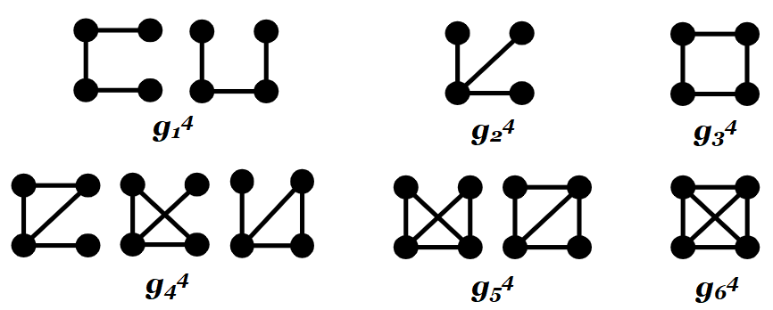
Figure 1. A list of different kinds of graphlets from the perspective of the bottom edge. From top to bottom, left to right, the graphlets are as follows: 3-paths ($g_{1}^{4}$), a 3-star ($g_{2}^{4}$), a 4-cycle ($g_{3}^{4}$), tailed triangles ($g_{4}^{4}$), diamonds ($g_{5}^{4}$), and a 4-clique ($g_{6}^{4}$).

In this work, we develop algorithms for the maintenance of size-$4$ graphlets. In doing so, we identify the local subgraph and count graphlets in the local subgraph using a state-of-the-art deterministic graphlet counting algorithm such as PGD.

PGD Algorithm:  The algorithm counts graphlets of size $3$ and $4$ in a static simple undirected graph. The algorithm leverages combinatorial arguments for different graphlets.

The algorithm iterates over the edges of the graph. Each iteration counts only a few graphlets and uses combinatorial arguments to derive the exact count of the rest of the graphlets in constant time. We leverage this algorithm to maintain the graphlet count in a dynamic network by appropriately choosing the subgraph and applying PGD on that subgraph with a guarantee that we can maintain the global graphlet count by counting graphlets in that subgraph only.

4. Algorithms

In this section, we design efficient algorithms for maintaining size-$4$ graphlets in a dynamic graph. First, we will describe the algorithm for an incremental batch where the goal is to update the graphlet count once a batch of new edges is added to the graph. Next, we will describe the algorithm for a fully dynamic batch consisting of edges for the addition and edges for the deletion. The algorithm’s objective is to maintain the frequency of all induced graphlets in the dynamic graph.

4.1. Baseline Algorithm

A straightforward algorithm for maintaining graphlet counts is to count all the graphlets in the updated graph using a state-of-the-art graphlet counting algorithm such as PGD (Ahmed et al., 2015b). We name this baseline as PGDN. This counting-from-scratch strategy is inefficient when the batch of edges touches a tiny portion of the graph. At the same time, the static algorithm for graphlet counting has to work on the much larger region of the graph for graphlet counting, which is required for maintaining the global count. An efficient technique would be to update the graphlet based on the count from the graph region where the change is located.

4.2. Incremental Stream

Now we will present an efficient algorithm for updating the graphlet count once a batch of edges $\mathcal{B}$ is added to the original graph $G$ through systematically exploring the subgraphs local to the changes in the graph. Once the subgraphs are explored, we count the graphlets in the local subgraphs. Finally, we aggregate these local counts to maintain the global graphlet counts in the updated graph.

Suppose a batch of new edges $\mathcal{B}=\{e_{1},e_{2},...,e_{l}\}$ is added to the graph $G=(V,E)$ and the updated graph is $G^{\prime}=G+\mathcal{B}=(V,E\cup\mathcal{B})$. This algorithm maintains two sub-graphs $\mathcal{G}_{a}$ and $\mathcal{G}_{b}$ of $\mathcal{G}$. It is easy to see that the diameter of size-$4$ graphlet is $3$, which occurs in the case of a $3$-path (Figure 1). Hence, the construction of $\mathcal{G}_{a}$ is as follows: For each edge $e_{i}=(u_{i},v_{i})$, we construct a subgraph $g_{i}$ induced by the vertex set $W_{i}=N_{3}(u_{i})\cup N_{3}(v_{i})$. Finally, $\mathcal{G}_{a}=g_{1}\cup g_{2}\cup...\cup g_{l}$. We construct $\mathcal{G}_{b}$ by removing all the edges in $\mathcal{B}$ from $\mathcal{G}_{a}$, formally, $\mathcal{G}_{b}=\mathcal{G}_{a}\setminus\mathcal{B}$.

The pseudocode is presented in Algorithm 1. The algorithm first updates the original graph $\mathcal{G}$ by adding the batch $\mathcal{B}$ to it. Next, it creates $\mathcal{G}_{a}$ and $\mathcal{G}_{b}$ and counts graphlets in $\mathcal{G}_{a}$ and $\mathcal{G}_{b}$. The following lemma shows that we can maintain the exact count of the graphlets using the graphlet counts in $\mathcal{G}_{a}$ and $\mathcal{G}_{b}$.

1

2Initialization:

3 Global Graphlet Counts $\mathcal{F}_{4}$ = [0, 0, 0, 0, 0, 0]

4 $\mathcal{G}_{a}$ Graphlet Counts $\mathcal{C}_{a}$ = [0, 0, 0, 0, 0, 0]

5 $\mathcal{G}_{b}$ Graphlet Counts $\mathcal{C}_{b}$ = [0, 0, 0, 0, 0, 0]

6

7foreach Batch $\mathcal{B}\in Inputs$ do

8      

9      $\mathcal{G}\leftarrow\mathcal{G}+\mathcal{B}$

10       Generate graph $\mathcal{G}_{a}$ = ($\mathcal{V}_{a}$, $\mathcal{E}_{a}$)

11       Generate graph $\mathcal{G}_{b}$ = ($\mathcal{V}_{b}$, $\mathcal{E}_{b}$)

12      

13      $\mathcal{C}_{a}\leftarrow PGD(\mathcal{G}_{a})$

14       $\mathcal{C}_{b}\leftarrow PGD(\mathcal{G}_{b})$

15       $\mathcal{C}^{\prime}\leftarrow\mathcal{C}_{a}-\mathcal{C}_{b}$

16       $\mathcal{F}_{4}\leftarrow\mathcal{F}_{4}+\mathcal{C}^{\prime}$

17      

18 end foreach

19return $\mathcal{F}_{4}$

Algorithm 1 IGC: Incremental Graphlet Counting

Lemma 0.

Suppose a batch of new edges $\mathcal{B}$ is added to the graph $\mathcal{G}=(\mathcal{V},\mathcal{E})$ and the graph is updated to $\mathcal{G}^{\prime}$. Then, $\mathcal{F}^{\mathcal{G}^{\prime}}_{4}=\mathcal{F}^{\mathcal{G}}_{4}+\mathcal{C}_{a}-\mathcal{C}_{b}$.

Proof.

There are three cases to consider:

case-1: all graphlets containing at least one new edge are added to the count. Observe that $\mathcal{C}_{a}$ captures all the graphlets that contain at least one new edge. Further, $\mathcal{C}_{b}$ will never capture any of these graphlets since they are missing some edges in $\mathcal{G}_{b}$. So, the count of every graphlet containing at least a new edge is added exactly once to the global count to update the answer.

case-2: all graphlets extended to a new graphlet by addition of edges are removed from the count. Observe that $\mathcal{C}_{b}$ captures all the graphlets as we remove all the new edges from $\mathcal{G}_{a}$ to get $\mathcal{G}_{b}$ and $\mathcal{C}_{a}$ will never capture the count of any such graphlets as they become non-induced once a batch is added. So, the count of these graphlets is subtracted exactly once.

case-3:  All graphlets that do not change after the addition of new edges do not contribute to the changes in the global graphlet counts. Since the graphlets were present before and after the addition of edges, they must be captured by both $\mathcal{C}_{a}$ and $\mathcal{C}_{b}$. So the count of every such graphlet is added exactly once and subtracted exactly once. So, the global count does not change. ∎

4.3. Fully Dynamic Stream

In this section, we describe our algorithm for maintaining global graphlet count in a fully dynamic setting where both insertion and deletion of edges are possible.

Suppose $\mathcal{B}=\mathcal{A}\cup\mathcal{D}$ is a batch of edges where $\mathcal{A}$ is a batch of edges to add and $\mathcal{D}$ is a batch of edges to delete. and Let, $H=\cup_{e=(u,v)\in\mathcal{A}\cup\mathcal{D}}G[\mathcal{N}_{3}(u)\cup\mathcal{N}_{3}(v)]$. Next we define $\mathcal{G}_{a}=(H\setminus\mathcal{D})\cup\mathcal{A}$ and $\mathcal{G}_{b}=(H\setminus\mathcal{A})\cup\mathcal{D}$ and then count the number of graphlets in $\mathcal{G}_{a}$ and $\mathcal{G}_{b}$. We use these counts in a systematic way to update the global graphlet count after processing the batch $\mathcal{B}$. The pseudocode is presented in Algorithm 2

1

2Initialization:

3 Global Graphlet Counts $\mathcal{F}_{4}$ = [0, 0, 0, 0, 0, 0]

4 $\mathcal{G}_{a}$ Graphlet Counts $\mathcal{C}_{a}$ = [0, 0, 0, 0, 0, 0]

5 $\mathcal{G}_{b}$ Graphlet Counts $\mathcal{C}_{b}$ = [0, 0, 0, 0, 0, 0]

6

7foreach Batch $\mathcal{B}=\mathcal{A}\cup\mathcal{D}\in Inputs$ do

8      

9      $H=\cup_{e\in\mathcal{A}\cup\mathcal{D}}G[\mathcal{N}_{3}(e)]$

10       $\mathcal{G}_{a}=(H\setminus\mathcal{D})\cup\mathcal{A}$

11       $\mathcal{G}_{b}=(H\setminus\mathcal{A})\cup\mathcal{D}$

12      

13      $\mathcal{C}_{a}\leftarrow PGD(\mathcal{G}_{a})$

14       $\mathcal{C}_{b}\leftarrow PGD(\mathcal{G}_{b})$

15       $\mathcal{C}^{\prime}\leftarrow\mathcal{C}_{a}-\mathcal{C}_{b}$

16       $\mathcal{F}_{4}\leftarrow\mathcal{F}_{4}+\mathcal{C}^{\prime}$

17       $\mathcal{G}\leftarrow\mathcal{G}\setminus\mathcal{D}\cup\{\mathcal{A}\}$

18      

19 end foreach

20return $\mathcal{F}_{4}$

Algorithm 2 FDGC: Fully Dynamic Graphlet Counting

Lemma 0.

Algorithm 2 correctly updates the global graphlet frequency.

Proof.

There are four types of graphlets. (1) type-1 graphlets containing edges in $\mathcal{D}$ but no edges in $\mathcal{A}$; (2) type-2 graphlets containing edges in both $\mathcal{A}$ and $\mathcal{D}$ (3) type-3 graphlets containing edges in $\mathcal{A}$ but no edge in $\mathcal{D}$ (4) type-4 graphlets containing edges neither from $\mathcal{A}$ nor from $\mathcal{D}$. All type-4 graphlets are captured by both $\mathcal{C}_{a}$ and $\mathcal{C}_{b}$, So $\mathcal{C}_{a}-\mathcal{C}_{b}=0$. Counts due to type-3 graphlets are captured in $\mathcal{C}_{a}$, added to the global count, but they are not captured by $\mathcal{C}_{b}$. type-2 graphlets are captured once in $\mathcal{C}_{a}$ and once in $\mathcal{C}_{b}$. So $\mathcal{C}_{a}-\mathcal{C}_{b}=0$. type-1 graphlets are removed, and therefore, corresponding counts are deleted, captured in $\mathcal{C}_{b}$, but not captured in $\mathcal{C}_{a}$. Transitioning of the graphlets as in case-2 of Lemma 4.1 are handled similarly as in Lemma 4.1. This completes the proof.

∎

5. Experiments

We evaluated our algorithm on large datasets to show the efficiency over the baseline PGDN. Every time we add a batch of edges and perform recomputation from scratch using the PGD. We show the description of the dataset in Table 1 taken from the Stanford SNAP (Leskovec and Krevl, 2014). We implemented all the algorithms in C++ and evaluated them in a system equipped with Intel(R) Xeon(R) W-2223 CPU $@$ $3.60$GHz with $4$ physical cores and $32$G RAM. We execute PGD with OpenMP to run in parallel.

Table 1. Characteristics of the Data sets

Dataset	$|V|$	$|E|$
WikiTalk (WT)	$2394385$	$4659565$
WikiVote (WV)	$7115$	$100762$
Soc-Pokec (SP)	$1632803$	$22301964$
soc-LiveJournal (LJ)	$4033137$	$27933062$

Batch creation: For the incremental batch computation, we group edges in a batch and execute the algorithms by inserting one batch at a time. For the fully dynamic batch, we create the batches as follows: First, we give $+$ive and $-$ive labels to the edges by sampling each edge with probability $p$ for selecting it to be a positive edge and putting the sampled edges in a queue. Later, we extract edges from the queue and sample them with probability $1-p$ to assign a $-$ive sign. This way, we create both positive and negative edges where the positive edge refers to the addition and the negative refers to the deletion. Next, we group them as before for creating batches. For our experiment, we choose $p=0.7$.

Computation on incremental batch: We empirically evaluated our algorithm IGC to show that IGC is much faster than PGDN on large graphs such as Soc-Pokec and soc-LiveJournal. This is because IGC counts graphlets on a relatively small size subgraph, which is local to the changes in the graph due to the batch update, while PGDN access the entire network built so far to count the graphlets. Also, the performance of IGC and PGDN is almost similar on WikiVote (Figure 2(a)) and WikiTalk (Figure 2(b)) because these networks are relatively small and sparse. Also, IGC needs to compute $3$-hop neighborhood for constructing the local subgraph, which is not substantially smaller than the original network where PGD work in the baseline. The results on batches of size $10$ and $100$ are shown in Figure 2 and Figure 3, respectively. In both cases, we observe that as the size of the graph increases with the increase in the edge counts, IGC is substantially faster than the baseline PGDN in two large networks Soc-Pokec (Figure 2(c) and Figure 3(b)) and soc-LiveJournal (Figure 2(d) and Figure 3(a)). This is as expected because PGDN accesses a larger graph each time compared to the size of the graph accessed by IGC.

Computation on fully dynamic batch: In a fully dynamic batch, we first removed the edges, which are both added and deleted, then executed Algorithm FDGC on the rest of the edges. Similar to the incremental stream, we observed similar behavior on two large networks Soc-Pokec and soc-LiveJournal as shown in Figure 4. Similar to the earlier observation, as the network size increases, the runtime of FDGC is significantly faster compared to PGDN than the initial state of the graph.

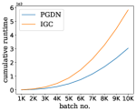
(a) WikiVote

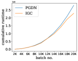
(b) WikiTalk

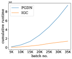
(c) Soc-Pokec

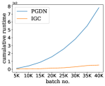
(d) soc-LiveJournal

Figure 2. Cumulative time to add insert only batches (of size $10$). Time at $y$-axis shows the overall time taken to add all the batches so far (represented by the batch number on the $x$-axis)

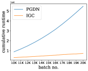
(a) soc-LiveJournal

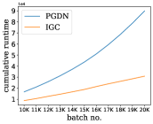
(b) Soc-Pokec

Figure 3. Cumulative time to add insert only batches (of size $100$). Time at $y$-axis shows the overall time taken to add all the batches so far (represented by the batch number on the $x$-axis)

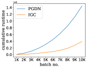
(a) soc-LiveJournal

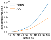
(b) Soc-Pokec

Figure 4. Cumulative time to add fully-dynamic batches (of size $100$). Time at $y$-axis shows the overall time taken to add all the batches so far (represented by the batch number on the $x$-axis)

6. Conclusion

In this work, we have developed an efficient algorithm for updating the counts of size-$4$ induced graphlets. Our algorithm is based on the exploration of subgraphs local to change in the graph by the fully dynamic stream of edges. We experimentally evaluated our algorithm to show the efficiency over the baseline.

References

- (1)
- Ahmed et al. (2015a) Nesreen K Ahmed, Jennifer Neville, Ryan A Rossi, and Nick Duffield. 2015a. Efficient graphlet counting for large networks. In 2015 IEEE international conference on data mining. IEEE, 1–10.
- Ahmed et al. (2015b) Nesreen K Ahmed, Jennifer Neville, Ryan A Rossi, and Nick Duffield. 2015b. Efficient graphlet counting for large networks. In 2015 IEEE International Conference on Data Mining. IEEE, 1–10.
- Bera and Seshadhri (2020) Suman K Bera and C Seshadhri. 2020. How the degeneracy helps for triangle counting in graph streams. In Proceedings of the 39th ACM SIGMOD-SIGACT-SIGAI Symposium on Principles of Database Systems. 457–467.
- Chen et al. (2022) Justin Y Chen, Talya Eden, Piotr Indyk, Honghao Lin, Shyam Narayanan, Ronitt Rubinfeld, Sandeep Silwal, Tal Wagner, David P Woodruff, and Michael Zhang. 2022. Triangle and Four Cycle Counting with Predictions in Graph Streams. In International Conference on Learning Representations.
- Danisch et al. (2018) Maximilien Danisch, Oana Balalau, and Mauro Sozio. 2018. Listing k-cliques in sparse real-world graphs. In Proceedings of the 2018 World Wide Web Conference. 589–598.
- Das et al. (2020) Apurba Das, Seyed-Vahid Sanei-Mehri, and Srikanta Tirthapura. 2020. Shared-memory parallel maximal clique enumeration from static and dynamic graphs. ACM Transactions on Parallel Computing (TOPC) 7, 1 (2020), 1–28.
- Dhulipala et al. (2021) Laxman Dhulipala, Quanquan C Liu, Julian Shun, and Shangdi Yu. 2021. Parallel batch-dynamic k-clique counting. In Symposium on Algorithmic Principles of Computer Systems (APOCS). SIAM, 129–143.
- Hanauer et al. (2022) Kathrin Hanauer, Monika Henzinger, and Qi Cheng Hua. 2022. Fully Dynamic Four-Vertex Subgraph Counting. In 1st Symposium on Algorithmic Foundations of Dynamic Networks.
- Harchaoui and Bach (2007) Zaid Harchaoui and Francis Bach. 2007. Image classification with segmentation graph kernels. In 2007 IEEE Conference on Computer Vision and Pattern Recognition. IEEE, 1–8.
- Janssen et al. (2012) Jeannette Janssen, Matt Hurshman, and Nauzer Kalyaniwalla. 2012. Model selection for social networks using graphlets. Internet Mathematics 8, 4 (2012), 338–363.
- Jha et al. (2015) Madhav Jha, C Seshadhri, and Ali Pinar. 2015. Path sampling: A fast and provable method for estimating 4-vertex subgraph counts. In Proceedings of the 24th international conference on world wide web. 495–505.
- Leskovec and Krevl (2014) Jure Leskovec and Andrej Krevl. 2014. SNAP Datasets: Stanford Large Network Dataset Collection. http://snap.stanford.edu/data.
- McGregor and Vorotnikova (2020) Andrew McGregor and Sofya Vorotnikova. 2020. Triangle and four cycle counting in the data stream model. In Proceedings of the 39th ACM SIGMOD-SIGACT-SIGAI Symposium on Principles of Database Systems. 445–456.
- Milenković et al. (2010) Tijana Milenković, Vesna Memišević, Anand K Ganesan, and Nataša Pržulj. 2010. Systems-level cancer gene identification from protein interaction network topology applied to melanogenesis-related functional genomics data. Journal of the Royal Society Interface 7, 44 (2010), 423–437.
- Milenković and Pržulj (2008) Tijana Milenković and Nataša Pržulj. 2008. Uncovering biological network function via graphlet degree signatures. Cancer informatics 6 (2008), CIN–S680.
- Mukherjee et al. (2018) Kingshuk Mukherjee, Md Mahmudul Hasan, Christina Boucher, and Tamer Kahveci. 2018. Counting motifs in dynamic networks. BMC systems biology 12, 1 (2018), 1–12.
- Pinar et al. (2017) Ali Pinar, C Seshadhri, and Vaidyanathan Vishal. 2017. Escape: Efficiently counting all 5-vertex subgraphs. In Proceedings of the 26th international conference on world wide web. 1431–1440.
- Pržulj et al. (2004) Natasa Pržulj, Derek G Corneil, and Igor Jurisica. 2004. Modeling interactome: scale-free or geometric? Bioinformatics 20, 18 (2004), 3508–3515.
- Rahman et al. (2014) Mahmudur Rahman, Mansurul Alam Bhuiyan, and Mohammad Al Hasan. 2014. Graft: An efficient graphlet counting method for large graph analysis. IEEE Transactions on Knowledge and Data Engineering 26, 10 (2014), 2466–2478.
- Rossi et al. (2018) Ryan A Rossi, Rong Zhou, and Nesreen K Ahmed. 2018. Estimation of graphlet counts in massive networks. IEEE transactions on neural networks and learning systems 30, 1 (2018), 44–57.
- Saha and Hasan (2015) Tanay Kumar Saha and Mohammad Al Hasan. 2015. Finding network motifs using MCMC sampling. (2015), 13–24.
- Seshadhri et al. (2013) Comandur Seshadhri, Ali Pinar, and Tamara G Kolda. 2013. Triadic measures on graphs: The power of wedge sampling. In Proceedings of the 2013 SIAM international conference on data mining. SIAM, 10–18.
- Shervashidze et al. (2009) Nino Shervashidze, SVN Vishwanathan, Tobias Petri, Kurt Mehlhorn, and Karsten Borgwardt. 2009. Efficient graphlet kernels for large graph comparison. In Artificial intelligence and statistics. PMLR, 488–495.
- Shin et al. (2020) Kijung Shin, Sejoon Oh, Jisu Kim, Bryan Hooi, and Christos Faloutsos. 2020. Fast, accurate and provable triangle counting in fully dynamic graph streams. ACM Transactions on Knowledge Discovery from Data (TKDD) 14, 2 (2020), 1–39.
- Stefani et al. (2017) Lorenzo De Stefani, Alessandro Epasto, Matteo Riondato, and Eli Upfal. 2017. Triest: Counting local and global triangles in fully dynamic streams with fixed memory size. ACM Transactions on Knowledge Discovery from Data (TKDD) 11, 4 (2017), 1–50.
- Vacic et al. (2010) Vladimir Vacic, Lilia M Iakoucheva, Stefano Lonardi, and Predrag Radivojac. 2010. Graphlet kernels for prediction of functional residues in protein structures. Journal of Computational Biology 17, 1 (2010), 55–72.
- Wang et al. (2012) Jianxin Wang, Yuannan Huang, Fang-Xiang Wu, and Yi Pan. 2012. Symmetry compression method for discovering network motifs. IEEE/ACM Transactions on Computational Biology and Bioinformatics 9, 6 (2012), 1776–1789.
- Wang et al. (2014) Pinghui Wang, John CS Lui, Bruno Ribeiro, Don Towsley, Junzhou Zhao, and Xiaohong Guan. 2014. Efficiently estimating motif statistics of large networks. ACM Transactions on Knowledge Discovery from Data (TKDD) 9, 2 (2014), 1–27.
- Wang et al. (2017) Pinghui Wang, Junzhou Zhao, Xiangliang Zhang, Zhenguo Li, Jiefeng Cheng, John CS Lui, Don Towsley, Jing Tao, and Xiaohong Guan. 2017. MOSS-5: A fast method of approximating counts of 5-node graphlets in large graphs. IEEE Transactions on Knowledge and Data Engineering 30, 1 (2017), 73–86.
- Zhang et al. (2013) Luming Zhang, Mingli Song, Zicheng Liu, Xiao Liu, Jiajun Bu, and Chun Chen. 2013. Probabilistic graphlet cut: Exploiting spatial structure cue for weakly supervised image segmentation. In Proceedings of the IEEE conference on computer vision and pattern recognition. 1908–1915.
- Zhang et al. (2012) Luming Zhang, Mingli Song, Qi Zhao, Xiao Liu, Jiajun Bu, and Chun Chen. 2012. Probabilistic graphlet transfer for photo cropping. IEEE Transactions on Image Processing 22, 2 (2012), 802–815.