Computation of the knot symmetric quandle and its application to the plat index of surface-links

Abstract.

A surface-link is a closed surface embedded in the 4-space, possibly disconnected or non-orientable. Every surface-link can be presented by the plat closure of a braided surface, which we call a plat form presentation. The knot symmetric quandle of a surface-link $F$ is a pair of a quandle and a good involution determined from $F$. In this paper, we compute the knot symmetric quandle for surface-links using a plat form presentation.

As an application, we show that for any integers $g\geq 0$ and $m\geq 2$, there exists infinitely many distinct surface-knots of genus $g$ whose plat indices are $m$.

1. Introduction

A surface-knot is a connected, closed surface embedded in $\mathbb{R}^{4}$, and a surface-link is a disjoint union of surface-knots. A 2-knot is an embedded 2-sphere in $\mathbb{R}^{4}$. Two surface-links are said to be equivalent to each other if one is ambiently isotopic to the other.

A quandle ([6, 13]) is a non-empty set $X$ with a binary operation satisfying three axioms corresponding to Reidemeister moves. Quandles are useful for studying oriented classical links and oriented surface-links. Kamada introduced a symmetric quandle ([9, 12]) as a pair of a quandle and its good involution. Symmetric quandles are useful tools for studying unoriented classical links and unoriented surface-links. As a generalization of the knot group and knot quandle, the knot symmetric quandle $X(F)$ of a surface-link $F$ was introduced and studied in [9, 10, 12].

In [16], Rudolph introduced a braided surface as an analogy of a braid in surface-knot theory. A braided surface of degree $m$ with $k$ branch points can be presented by an $r$-tuple of classical $m$-braids, called a braid system. See Definition 2.3. In [20], it is shown that every surface-link has a plat form presentation, which is the plat closure of an adequate braided surface. See [20] or Section 2.2 for the definition and details.

The aim of this paper is to compute the knot symmetric quandle of a surface-link by using a braid system via a plat form presentation.

Theorem 1.1.

Let $F$ be a surface-link, and $S$ be an adequate braided surface $S$ of degree $2m$ providing a plat form for $F$. Let $(\beta_{1}^{-1}\sigma^{\varepsilon_{1}}_{k_{1}}\beta_{1},\ldots,\beta_{r}^{-1}\sigma^{\varepsilon_{r}}_{k_{r}}\beta_{r})$ be a braid system of $S$, where $\sigma_{i}$ is Artin’s generator of $B_{2m}$, $\beta_{i}\in B_{2m}$, $\varepsilon_{i}\in\{\pm 1\}$, and $1\leq k_{i}\leq 2m-1$. Then the knot symmetric quandle $X(F)$ has the following presentation:

$$\left\langle x_{1},\ldots,x_{2m}~{}\begin{array}[]{|c}\mathrm{Artin}(\beta_{j})(x_{k_{i}})=\mathrm{Artin}(\beta_{j})(x_{k_{i}+1})~{}(i=1,\ldots,r)\\ x_{2j-1}=x_{2j}^{-1}~{}(j=1,\ldots,m)\end{array}\right\rangle_{\mathrm{sq}},$$

where $\mbox{Artin}(\beta)$ is Artin’s automorphism on the free symmetric quandle.

We remark that the knot group of $F$ has a similar presentation (Remark 4.8).

The plat index ([20]) of a surface-link $F$, denoted by $\mbox{Plat}(F)$, is defined as the half of the minimum number of the degree of adequate braided surfaces whose plat closures are equivalent to $F$. By Theorem 1.1, we obtain the following inequality between the plat index of $F$ and the symmetric quandle coloring number of $F$.

Theorem 1.2.

For any surface-link $F$ and any finite symmetric quandle $X$, the following inequality holds:

$$\log_{(\#X)}\mathrm{col}_{X}(F)\leq\mathrm{Plat}(F),$$

where $\#X$ is the order of $X$ and $\mbox{col}_{X}(F)$ is the $X$-coloring number of $F$.

It is known that the plat index of a surface-link $F$ is 1 if and only if $F$ is either a trivial 2-knot or a trivial non-orientable surface-knot ([20]). Using Theorems 1.1 and 1.2, we show the following theorem.

Theorem 1.3.

For any integers $g\geq 0$ and $m\geq 2$, there exist infinitely many distinct orientable surface-knots of genus $g$ whose plat indices are $m$.

This paper is organized as follows: In section 2, we introduce a braided surface, a braid system, and a plat form presentation for a surface-link. In section 3, we review a quandle and a symmetric quandle. We prove Theorem 1.1 in section 4, and we prove Theorem 1.3 in section 5.

2. A plat form presentation

2.1. A plat form presentation for classical links

Throughout this paper, we work in the PL category or the smooth category and assume that surface-links are locally flat in the PL category. Let $n$ be a positive integer, $I=[0,1]$ be the interval, $D^{2}$ be the square $I^{2}$ or a $2$-disk in $\mathbb{R}^{2}$. Let $Q_{n}$ be the subset of $n$ points in $D^{2}$ consisting of $q_{k}=\left({1}/{2},{k}/{(n+1)}\right)\in I\times I=D^{2}$ for $k=1,2,\cdots,n$.

The braid group $B_{n}$ is the fundamental group $\pi_{1}(\mathcal{C}_{n},Q_{n})$ of the configuration space $\mathcal{C}_{n}$ of $n$ points of $\mathrm{Int}\,D^{2}$ with base point $Q_{n}$. An element of $B_{n}$ is called an $n$-braid. A geometric $n$-braid is a union of $n$ intervals $\beta$ embedded in $D^{2}\times I$ such that each component meets every open disk $\mathrm{Int}\,D^{2}\times\{t\}$ ($t\in I$) transversely at a single point, and $\partial\beta=Q_{n}\times\{0,1\}$. We identify an $n$-braid with an equivalence class of a geometric $n$-braid. We denote by $\sigma_{1},\sigma_{2},\dots,\sigma_{n-1}$ the standard generators of $B_{n}$ or their representatives due to Artin ([1]).

Definition 2.1 ([3]).

A wicket is a semicircle in $D^{2}\times I$ that meets $D^{2}\times\{0\}$ orthogonally at its endpoints in $\mathrm{Int}\,D^{2}$. A configuration of $m$ wickets is a disjoint union of $m$ wickets in $D^{2}\times I$.

The enhanced boundary of a configuration of $m$ wickets $w$, denoted by $\partial w$, is the boundary of $w$, which is $2m$ points of $\mathrm{Int}\,D^{2}$, equipped with a partition into $m$ pairs of points such that each pair of points is the boundary of a wicket of $w$. $|\partial w|$ denotes the $2m$ points $\partial w$ forgetting the partition. Then two configurations $w$, $w^{\prime}$ are the same if they have the same enhanced boundary, $\partial w=\partial w^{\prime}$.

The set $Q_{2m}$ equipped with the partition $\{\{q_{1},q_{2}\},\dots,\{q_{2m-1},q_{2m}\}\}$ bounds a unique configuration of $m$ wickets, which we call the standard configuration of $m$ wickets and denote it by $w_{0}$.

Let $\beta$ be a geometric $2m$-braid in $D^{2}\times I\subset\mathbb{R}^{2}\times\mathbb{R}=\mathbb{R}^{3}$. The plat closure of $\beta$, denoted by $\widetilde{\beta}$, is a link obtained by attaching two copies of the standard configurations of $m$ wickets to $\beta$ as shown in Figure 1. Similarly, a link $L$ is in a plat form if $L=\widetilde{\beta}$ for some $2m$-braid $\beta$. Every link is equivalent to a link in a plat form.

Figure 1. The plat closure of a braid.

2.2. Braided surfaces and braid systems

Let $D_{1}$ and $D_{2}$ be the squares $I^{2}$ in $\mathbb{R}^{2}$ and let $\mathrm{pr}_{i}:D_{1}\times D_{2}\to D_{i}$ $(i=1,2)$ be the $i$-th factor projection. Let $y_{0}$ be a fixed base point of $D_{2}$ with $y_{0}\in\partial D_{2}$.

Definition 2.2 ([16], [19]).

A surface $S$ embedded in $D_{1}\times D_{2}$ is a (pointed) braided surface of degree $n$ if $S$ satisfies the following conditions:

1. $\pi_{S}=\mathrm{pr}_{2}|_{S}:S\to D_{2}$ is a branched covering map of degree $n$.

2. $\partial S$ is the closure of an $n$-braid in the solid torus $D_{1}\times\partial D_{2}$.

3. $\mathrm{pr_{1}}(\pi_{S}^{-1}(y_{0}))=Q_{n}$.

A $2$-dimensional braid of degree $n$ is a braided surface $S$ of degree $n$ such that $\mathrm{pr_{1}}(\pi_{S}^{-1}(y))=Q_{n}$ for all $y\in\partial D_{2}$.

Throughout this paper, we assume that every braided surface of degree $n$ is simple, that is, the preimage of each branch locus of $\pi_{S}$ consists of $n-1$ points. An orientation of $S$ is compatible with an orientation of $D_{2}$ if for each regular point $x\in S$ of $\pi_{S}$, the orientation of $S$ at $x$ is coherent with the orientation of $D_{2}$ at $\pi_{S}(x)$ via $\pi_{S}$. Unless otherwise stated, an orientation of $S$ is always chosen to be compatible with an orientation of $D_{2}$.

For two braided surfaces of the same degree, they are said to be equivalent if they are ambiently isotopic by an isotopy $\{h_{s}\}_{s\in I}$ of $D_{1}\times D_{2}$ such that each $h_{s}$ ($s\in I$) is fiber-preserving when we regard $D_{1}\times D_{2}$ as the trivial $D_{1}$-bundle over $D_{2}$, and the restriction of $h_{s}$ to ${\mathrm{pr}_{2}^{-1}(y_{0})}$ is the identity map.

Next, we recall the braid monodromy and a braid system of a braided surface $S$. Let $\Sigma(S)\subset D_{2}$ be the branch locus of $\pi_{S}$. For a loop $c:(I,\partial I)\to(D_{2}\setminus\Sigma(S),y_{0})$, we define a loop $\rho_{S}(c):(I,\partial I)\to(\mathcal{C}_{n},Q_{n})$ as $\rho_{S}(c)(t)=\mathrm{pr}_{1}(\pi_{S}(c(t))^{-1})$. Then this map induces a homomorphism $\rho_{S}:\pi_{1}(D_{2}\setminus\Sigma(S),y_{0})\to B_{n}=\pi_{1}(\mathcal{C}_{n},Q_{n})$ by $\rho_{S}([c])=[\rho_{S}(c)]$, which is called the braid monodromy of $S$.

Let $r\geq 1$ be a positive integer. A Hurwitz arc system in $D_{2}$ (with the base point $y_{0}$) is an $r$-tuple $\mathcal{A}=(\alpha_{1},\cdots,\alpha_{r})$ of oriented simple arcs in $D_{2}$ such that

1. $\alpha_{i}\cap\partial D_{2}=\partial\alpha_{i}\cap\partial D_{2}=\{y_{0}\}$ and this is the terminal point of $\alpha_{i}$,

2. $\alpha_{i}\cap\alpha_{j}=\{y_{0}\}$ ($i\neq j$), and

3. $\alpha_{1},\ldots,\alpha_{r}$ appears in this order around the base point $y_{0}$.

The starting point set of $\mathcal{A}$ is the set of initial points of $\alpha_{1},\ldots,\alpha_{r}$.

Let $\mathcal{A}=(\alpha_{1},\cdots,\alpha_{r})$ be a Hurwitz arc system with the starting point set $\Sigma(S)$ and $N_{i}$ be a (small) regular neighborhood of the starting point of $\alpha_{i}$ and let $\overline{\alpha_{i}}$ be an oriented arc obtained from $\alpha_{i}$ by restricting to $D_{2}\setminus\mathrm{Int}\,N_{i}$. For each $\alpha_{i}$, let $\gamma_{i}$ be a loop $\overline{\alpha_{i}}^{-1}\cdot\partial N_{i}\cdot\overline{\alpha_{i}}$ in $D_{2}\setminus\Sigma(S)$ with base point $y_{0}$, where $\partial N_{i}$ is oriented counter-clockwise. Then $\pi_{1}(D_{2}\setminus\Sigma(S),y_{0})$ is the free group generated by $[\gamma_{1}],[\gamma_{2}],\ldots,[\gamma_{r}]$.

Definition 2.3 ([16, 8]).

A braid system of $S$ is an $r$-tuple $b_{S}$ of $n$-braids defined as

$$b_{S}~{}=~{}(\rho_{S}([\gamma_{1}])\ldots,\rho_{S}([\gamma_{r}])).$$

It is known that $\rho_{S}([\gamma_{i}])$ is a conjugation of some generator $\sigma_{k_{i}}^{\varepsilon_{i}}$, where $\varepsilon_{i}\in\{\pm 1\}$ is called the sign of the branch point whose projection is the starting point of $\alpha_{i}$.

We do not mention a chart description of $S$ in this paper. However, it is worth noting that a braid system of $S$ can be easily obtained from its chart description, see [8] for details.

Let $G$ be a group and $G^{r}$ the set of $r$-tuples of elements of $G$. The slide action of the braid group $B_{r}$ on $G^{r}$ is a left group action defined by

$$\mathrm{slide}(\sigma_{j})(g_{1},\ldots,g_{r})~{}=~{}(g_{1},\ldots,g_{j-1},g_{j}g_{j+1}g_{j}^{-1},g_{j},g_{j+2},\ldots,g_{r})$$

for $(g_{1},\ldots,g_{r})\in G^{r}$ and $\sigma_{j}\in B_{r}$. Two elements of $G^{r}$ are said to be Hurwitz equivalent (or slide equivalent) if their orbits of slide action are the same.

It is known that a Hurwitz equivalence class of a braid system of $S$ is uniquely determined by the equivalence class of $S$(cf. [8, 14, 17]) although a braid system of $S$ depends on the choice of a Hurwitz arc system $\mathcal{A}$.

2.3. A plat form presentation for surface-links

For an integer $m\geq 1$, $\mathcal{W}_{m}$ denotes the space consisting of all configurations of $m$ wickets. For a loop $f:(I,\partial I)\to(\mathcal{W}_{m},w_{0})$, the geometric $2m$-braid $\beta_{f}$ is defined as

$$\beta_{f}~{}=~{}\bigcup_{t\in I}|\partial f(t)|\times\{t\}\subset D\times I.$$

Definition 2.4.

A geometric $2m$-braid $\beta$ is adequate if $\beta=\beta_{f}$ for some loop $f:(I,\partial I)\to(\mathcal{W}_{m},w_{0})$.

Since a configuration of wickets is unique for its enhanced boundary, two loops $f,g:(I,\partial I)\to(\mathcal{W}_{m},w_{0})$ are the same if $\beta_{f}=\beta_{g}$.

Hilden’s subgroup $K_{2m}$ is defined as the subgroup of $B_{2m}$ generated by the following elements ([5], cf. [2]):

$$K_{2m}~{}=~{}\left\langle\begin{array}[]{c|c}\sigma_{1},~{}\sigma_{2}\sigma_{1}\sigma_{3}\sigma_{2},~{}\sigma_{2j}\sigma_{2j-1}\sigma_{2j+1}^{-1}\sigma_{2j}^{-1}&j=1,\dots,m-1\end{array}\right\rangle.$$

Two $2m$-braids $\sigma_{2j}\sigma_{2j-1}\sigma_{2j+1}\sigma_{2j}$ and $\sigma_{2j}\sigma_{2j-1}\sigma_{2j+1}^{-1}\sigma_{2j}^{-1}$ are denoted by $\tau_{j}$ and $\upsilon_{j}$, respectively. We remark that $\sigma_{2i-1},\tau_{j},\upsilon_{j}\in K_{2m}$ for $i=1,\ldots,m$ and $j=1,\ldots,m-1$.

Figure 2. Generators of Hilden’s subgroup $K_{4}$ ($m=2$)

Brendle and Hatcher [3] showed that $\pi_{1}(\mathcal{W}_{m},w_{0})$ is isomorphic to $K_{2m}$. Such an isomorphism is given by sending $[f]\in\pi_{1}(\mathcal{W}_{m},w_{0})$ to $[\beta_{f}]\in B_{2m}$. We remark that Hilden’s subgroup $K_{2m}$ consists of elements of $B_{2m}$ represented by some adequate $2m$-braid.

We fix a loop $\mu:(I,\partial I)\to(\partial D_{2},y_{0})$ which runs once on $\partial D_{2}$ counter-clockwise. For a braided surface $S$ of degree $n$, let $\beta_{S}$ be the geometric $n$-braid in $D_{1}\times I$ defined by

$$\beta_{S}~{}=~{}\bigcup_{t\in I}\mathrm{pr}_{1}(\pi_{S}^{-1}(\mu(t)))\times\{t\},$$

where $\pi_{S}:S\to D_{2}$ is the simple branched covering map induced from $S$. Then $\partial S$ is the closure of $\beta_{S}$ in $D_{1}\times(I/\partial I)\cong D_{1}\times\partial D_{2}$.

Definition 2.5.

A braided surface $S$ in $D_{1}\times D_{2}$ is adequate if $\beta_{S}$ is adequate.

The degree of an adequate braided surface is even and every 2-dimensional braid of even degree is adequate. By definition, a loop $f:(I,\partial I)\to(\mathcal{W}_{m},w_{0})$ satisfying $\beta_{S}=\beta_{f}$ is unique for $S$, thus we denote it by $f_{S}$.

We assume $D_{1}\times D_{2}\subset\mathbb{R}^{2}\times\mathbb{R}^{2}=\mathbb{R}^{4}$. Let $N$ be a regular neighborhood of $\partial D_{2}$ in $\mathbb{R}^{2}\setminus\mathrm{Int}\,{D_{2}}$, which is homeomorphic to an annulus $I\times S^{1}$. We identify $N$ with $I\times S^{1}$ by a fixed identification map $\phi:I\times S^{1}\to N$ such that $\phi(0,p(t))=\mu(t)\in\partial D_{2}$ for all $t\in I$, where $p:I\to S^{1}=I/\partial I$ is the quotient map.

Definition 2.6.

Let $S$ be an adequate braided surface of degree $2m$. The surface of wicket type associated with $S$ is a properly embedded surface $A_{S}$ in $D_{1}\times N$ defined by

$$A_{S}~{}=~{}\bigcup_{t\in I}f_{S}(t)\times\{p(t)\}~{}\subset~{}(D\times I)\times S^{1}~{}=~{}D_{1}\times N.$$

The surface $A_{S}$ is uniquely determined by $S$ since the loop $f_{S}$ is unique for $S$. Furthermore, the intersection of $S$ with $A_{S}$ is equal to their boundaries; $S\cap A_{S}=\partial S=\partial A_{S}$. Thus, we obtain a surface-link from an adequate braided surface $S$ by taking the union $S\cup A_{S}$.

Definition 2.7.

Let $S$ be an adequate braided surface, and $A_{S}$ be the surface of wicket type associated with $S$. The plat closure of $S$, denoted by $\widetilde{S}$, is the union $S\cup A_{S}$ in $\mathbb{R}^{4}$.

Definition 2.8.

A surface-link is said to be in a plat form if it is the plat closure of some adequate braided surface. Moreover, a surface-link is said to be in a genuine plat form if it is the plat closure of some $2$-dimensional braid.

In [20], it is shown that every surface-link has a plat form presentation and that every orientable surface-link has a genuine plat form presentation.

Definition 2.9.

Let $F$ be a surface-link. The plat index of $F$ is defined as the half of the minimum degree of adequate braided surfaces whose plat closures are equivalent to $F$, denoted by $\mbox{Plat}(F)$. Similarly, the genuine plat index of $F$ is defined as the half of the minimum degree of 2-dimensional braids of even degree whose plat closures are equivalent to $F$, denoted by $\mbox{g.Plat}(F)$.

3. Symmetric quandles and symmetric quandle presentations

In this section, we introduce the notions of symmetric quandles and their presentation.

Definition 3.1 ([6, 13]).

A quandle is a nonempty set $X$ with a binary operation $(x,y)\mapsto x^{y}$ that satisfies the following three conditions:

• $x^{x}=x$ for any $x\in X$,

• there is a unique binary operation $(x,y)\mapsto x^{y^{-1}}$ such that $(x^{y})^{y^{-1}}=(x^{y^{-1}})^{y}=x$ for any $x,y\in X$, and

• $(x^{y})^{z}=(x^{z})^{(x^{y})}$ for any $x,y,z\in X$.

A rack is a nonempty set with a binary operation that satisfies (Q2) and (Q3).

Definition 3.2 ([9, 12]).

Let $X$ be a quandle. An involution map $\rho:X\to X$ is called a good involution if $\rho$ satisfies the following two conditions:

• $\rho(x^{y})=\rho(x)^{y}$ for any $x,y\in X$, and

• $x^{\rho(y)}=x^{y^{-1}}$ for any $x,y\in X$.

A symmetric quandle is a pair $(X,\rho)$ of a quandle $X$ and its good involution $\rho$.

For symmetric quandles $(X,\rho)$ and $(X^{\prime},\rho^{\prime})$, a map $f:X\to X^{\prime}$ is a symmetric quandle homomorphism if $f$ satisfies $f(x^{y})=f(x)^{f(y)}$ and $f(\rho(x))=\rho^{\prime}(f(x))$ for any $x,y\in X$.

We write $x^{-1}$ and $x^{-y}$ for $\rho(x)$ and $\rho(x^{y})$, respectively, when the good involution of $(X,\rho)$ is clearly. Then, $(x^{y})^{-1}=(x^{-1})^{y}=x^{-y}$ and $x^{(y^{-1})}=x^{y^{-1}}$ hold for $x,y\in X$.

Example 3.3.

The dihedral quandle $R_{p}$ of order $p$ is the cyclic group of order $p$ with a binary operator defined by $a^{b}=2b-a$ for $a,b\in R_{p}$. For every positive integer $p$, the identity map $\mathop{\mathrm{id}}\nolimits_{R_{p}}:R_{p}\to R_{p}$ is a good involution of $R_{p}$. Thus, $(R_{n},\mathop{\mathrm{id}}\nolimits_{R_{n}})$ is a symmetric quandle.

In general, a kei (or an involutive quandle) is a quandle $X$ such that $(x^{y})^{y}=x$ for any $x,y\in X$. It is known that the identity map $\mathop{\mathrm{id}}\nolimits_{X}$ on a quandle $X$ is a good involution if and only if $X$ is a kei ([12]).

Example 3.4 ([12]).

Let $K$ be a properly embedded $n$-submanifold in $(n+2)$-manifold $W$, $N(K)$ be a regular neighborhood of $K$ in $W$, $E(K)=\mathrm{cl}(W\setminus N(K))$ be the exterior of $K$, and $*$ be a fixed based point of $E(K)$. A noose of $K$ is a pair $(D,\alpha)$ of an oriented meridional disk $D$ of $K$ and an oriented arc $\alpha$ in $E(K)$ connecting from a point of $\partial D$ to $*$. The knot full quandle ([9, 12]) of $(W,K)$ is a quandle consisting of homotopy classes $[(D,\alpha)]$ of nooses of $K$ with a binary operator defined by

$$[(D_{1},\alpha_{1})]^{[(D_{2},\alpha_{2})]}=[(D_{1},\alpha_{1}\cdot\alpha_{2}^{-1}\cdot\partial D_{2}\cdot\alpha_{2})].$$

Note that the knot full quandle of $K$ is independent of the choice of the based point $*$ when $W$ is connected. Thus we denote it by $\widetilde{Q}(W,K)$ or simply $\widetilde{Q}(K)$. Here, ”full” means that $\widetilde{Q}(K)$ contains both nooses of $(D,\alpha)$ and $(-D,\alpha)$, where $-D$ is $D$ with the reverse orientation. Let $\rho$ be an involution map of $\widetilde{Q}(K)$ defined by $\rho([(D,\alpha)])=[(-D,\alpha)]$, then $\rho$ is a good involution. We call $(\widetilde{Q}(K),\rho)$ the knot symmetric quandle of $K$, denoted by $X(W,K)$ or simply $X(K)$.

For a pair $(W,K)$ and a symmetric quandle $X$, let $\mbox{Col}_{X}(F)$ be the set of symmetric quandle homomorphisms from $X(W,K)$ to $X$. The $X$-coloring number of $(W,K)$ is defined as the cardinal number of $\mbox{Col}_{X}(F)$, denoted by $\mbox{col}_{X}(W,K)$ or $\mbox{col}_{X}(K)$.

Example 3.5 ([10]).

Let $A$ be a non-empty set and $F(A)$ be the free group on $A$. We put $\overline{A}=\{a^{-1}\in F(A)~{}|~{}a\in A\}$ and suppose that $A$ and $\overline{A}$ are disjoint. Then $\widetilde{\mbox{FR}}(A)=(A\cup\overline{A})\times F(A)$ is a rack equipped with a binary operator given by $(a,w)^{(b,z)}=(a,wz^{-1}bz)$ for $(a,w),(b,z)\in\widetilde{\mbox{FR}}(A)$.

Let $\sim_{sq}$ be the equivalence relation on $\widetilde{\mbox{FR}}(A)$ generated by $(a,w)\sim_{sq}(a,a^{aw})$ for $a\in(A\cup\overline{A})$ and $w\in F(A)$. Then the rack operation on $\widetilde{\mbox{FR}}(A)$ induces a quandle operation on $\widetilde{\mbox{FQ}}(A)=\widetilde{\mbox{FR}}(A)/\sim_{sq}$. An involution map $\rho_{A}:\widetilde{\mbox{FQ}}(A)\to\widetilde{\mbox{FQ}}(A)$ given by $\rho(a^{\pm 1},w)\mapsto(a^{\mp 1},w)$ is a good involution of $\widetilde{\mbox{FQ}}(A)$. $(\widetilde{\mbox{FQ}}(A),\rho_{A})$ is called the free symmetric quandle on $A$, denoted by $\mbox{FSQ}(A)$. For $a\in A$ and $w\in F(A)$, elements $(a,w)$ and $(a^{-1},w)$ in $\mbox{FSQ}(A)$ are denoted by $a^{w}$ and $a^{-w}$, respectively. For $a\in(A\cup\overline{A})$ and the identity $1\in F(A)$, we simply write $a$ for $a^{1}\in\mbox{FSQ}(A)$.

Let $R$ be a subset of $\mbox{FSQ}(A)\times\mbox{FSQ}(A)$. We denote $R_{0}$ as $R$. For $n\geq 1$, we expand $R_{n-1}$ to $R_{n}$ by the following moves:

1. For every $x\in FQ(A)$, add $(x,x)\in R_{n}$.

2. For every $(x,y)\in R_{n-1}$, add $(y,x)\in R_{n}$.

3. For every $(x,y),(y,z)\in R_{n-1}$, add $(x,z)\in R_{n}$.

4. For every $(x,y)\in R_{n-1}$ and $a\in A$, add $(x^{a},y^{a}),(x^{-a},y^{-a})\in R_{n}$.

5. For every $(x,y)\in R_{n-1}$ and $t\in\mbox{FQ}(A)$, add $(t^{x},t^{y}),(t^{-x},t^{-y})\in R_{n}$.

6. For every $a\in A$, add $(a^{a},a)\in R_{n}$.

Then the union $\langle\langle R\rangle\rangle_{sq}=\bigcup_{n\geq 0}R_{n}$ is called the set of symmetric quandle consequences of $R$, which is the smallest congruence containing $R$ with respect to the axioms of a symmetric quandle ([10]). An element of $\langle\langle R\rangle\rangle_{sq}$ is called a consequence of $R$. Then, the quandle operation and the good involution on $\mbox{FSQ}(A)$ induce a quandle operation and a good involution on $\mbox{FSQ}(A)/\langle\langle R\rangle\rangle_{sq}$. This symmetric quandle is denoted by $\langle A~{}|~{}R\rangle_{sq}$.

Definition 3.6 ([10]).

The symmetric quandle $\langle A~{}|~{}R\rangle_{sq}$ is a symmetric quandle presentation (or simply presentation) of $X$ if $X$ is isomorphic to $\langle A~{}|~{}R\rangle_{sq}$.

Each element $a\in A$ is called a generator of $X$ and each element $r\in R$ is called a relator of $X$. A presentations $\langle A~{}|~{}R\rangle_{sq}$ is finite if both $A$ and $R$ are finite.

We usually write $(a^{w},b^{w})\in\langle\langle R\rangle\rangle_{sq}$ as an equation $a^{w}=b^{z}$.

The following lemmas are proved for racks and quandles (cf. [11]), and these proofs can be extended to the case of symmetric quandles.

Lemma 3.7 (cf. [11, Proposition 8.6.1]).

Let $A$ be a non-empty set and $X$ be a symmetric quandle. For a map $f:A\to X$, there is a unique homomorphism $f_{\sharp}:\mbox{FSQ}(A)\to X$ such that $f=f_{\sharp}\circ\iota$, where $\iota:A\to\mbox{FSQ}(A)$ is the natural inclusion map.

Lemma 3.8 (cf. [11, Lemma 8.6.3]).

Let $X$ be a symmetric quandle with a presentation $\langle A~{}|~{}R\rangle_{sq}$. For a symmetric quandle $Y$, a map $f:A\to Y$ extends to a homomorphism $f:X\to Y$ if and only if $f(a)^{f(w)}=f(b)^{f(z)}$ holds for $(a^{w},b^{z})\in R$.

Definition 3.9 (cf. [4]).

Let $X$ be a symmetric quandle with a presentation $\langle A~{}|~{}R\rangle_{sq}$. The following four moves are called Tietze moves on a symmetric quandle presentation.

1. Add a consequence of $R$ to $R$.

2. Delete a consequence of other relators from $R$.

3. Introduce a new generator $a$ and a new relator $(a,r)$ to $A$ and $R$, respectively, where $r$ is an element of $F(A)$.

4. Delete a generator $a$ and a relator $(a,r)$ from $A$ and $R$, respectively, where $(a,r)$ is a consequence of other relators and $a$ does not occur in other relators in $R$.

Note that (T2) and (T4) are inverse moves of (T1) and (T3), respectively. Fenn and Rourke [4] proved Tietze move theorem for racks, and their proof can be extended for symmetric quandles.

Proposition 3.10 (cf. [4]).

Any two finite presentations of a symmetric quandle are related by a finite sequence of Tietze moves.

4. Computation of the knot symmetric quandles

In this section, we compute the knot symmetric quandle for surface-links using a plat form presentation.

4.1. Diagrams and semi-sheets

First, we introduce a diagram and a semi-sheet for an $n$-submanifold $K$ embedded in $\mathbb{R}^{n+2}$. Without loss of generality, we may suppose that $K$ is in general position with respect to the projection $\pi:\mathbb{R}^{n+2}=\mathbb{R}\times\mathbb{R}^{n+1}\to\mathbb{R}^{n+1}$. Let $\Delta_{K}$ be the closure of the singular set of $\pi(K)$;

$$\Delta_{K}=\mathrm{cl}(\{x\in\pi(K)\in\mathbb{R}^{n+1}~{}|~{}\#(\pi^{-1}(x)\cap K)>1\}).$$

A diagram $D_{K}$ of $K$ is a union of $\mathrm{cl}(\pi(K)\setminus N(\Delta_{K}))$ and the projection of the upper preimage of $N(\Delta_{K})$, where $N(\Delta_{K})$ is a regular neighborhood of $\Delta_{K}$. Figure 3 depicts local models of a surface-link diagram ($n=2$).

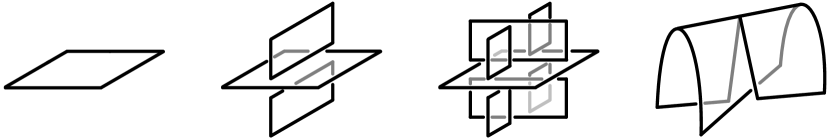
Figure 3. Local models of a diagram of a surface-link.

Each connected component of $\mathrm{cl}(\pi(K)\setminus N(\Delta_{K}))$ is called a semi-sheet of $D_{K}$. Figure 4 depicts local models of semi-sheets of a surface-link diagram ($n=2$). We also call it a semi-arc when $K$ is a classical link.

Figure 4. Local models of semi-sheets of a surface-link.

When we regard $\Delta_{K}$ as a stratified complex, each $(n-1)$-dimensional stratum of $\Delta_{K}$ consists of transverse double points (cf. [15]), which is called the double point stratum of $D_{K}$. Each double point stratum of a classical link diagram corresponds to a crossing, and each double point stratum of a surface-link diagram corresponds to a double point curve.

Let $x_{1},\ldots,x_{n}$ be semi-sheets of $D_{K}$. Since semi-sheets are orientable ([7]), we give them orientations arbitrarily. For semi-sheets $x_{i},x_{j},x_{s},x_{t}$ around a double point stratum of $D_{K}$ as in Figure 5, we define the A-relation and the B-relation as follows: Assume that $x_{i}$ and $x_{j}$ are upper semi-sheets and that $x_{s}$ and $x_{t}$ are lower semi-sheets (Figure 5). The A-relation is defined as $x_{i}=x_{j}$ if orientations of $x_{i}$ and $x_{j}$ are coherent (Figure 6-(a)) and $x_{i}=x_{j}^{-1}$ otherwise (Figure 6-(b)), where normal vectors on semi-sheets described in Figure 6 represent their orientations (cf. [10]). Suppose that the normal vector of $x_{i}$ is directed from $x_{s}$ to $x_{t}$. The B-relation is defined as $x_{t}=x_{s}^{x_{i}}$ if orientations of $x_{s}$ and $x_{t}$ are coherent (Figure 6-(c)) and $x_{t}^{-1}=x_{s}^{x_{i}}$ otherwise (Figure 6-(d)). The set of the A-relations and B-relations of $D_{K}$ is denoted by $\mbox{A-rel}_{D_{K}}$ and $\mbox{B-rel}_{D_{K}}$, respectively.

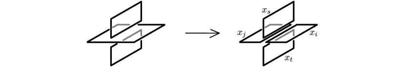
Figure 5. Semi-sheets around a double point strata and their labeling.

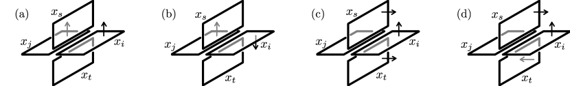
Figure 6. The A-relation and the B-relation.

Using these relations, we define a symmetric quandle $X(D_{K})$ by

$$X(D_{K})~{}=~{}\left\langle x_{1},\ldots,x_{s}~{}\begin{array}[]{|c}\mbox{A-rel}_{D_{K}},\mbox{B-rel}_{D_{K}}\end{array}\right\rangle_{\mathrm{sq}}.$$

It is known that $X(D_{K})$ is a well-defined symmetric quandle although the A-relation and the B-relation depend on the choice of orientations and labeling of semi-sheets ([10]).

Proposition 4.1 ([10]).

The knot symmetric quandle $X(K)$ is isomorphic to $X(D_{K})$.

The isomorphism between $X(D_{K})$ and $X(K)$ is given in [10, Theorem 4.11] as follows: Let $\Sigma=\mathrm{cl}(\pi(K)\setminus N(\Delta_{K}))$ be the union of semi-sheets of $D_{K}$. We may assume that

$$K\cap[0,\infty)\times\mathbb{R}^{n+1}~{}=~{}[0,1]\times\partial\Sigma\cup\{1\}\times\Sigma.$$

We take a base point $*$ of $\mathbb{R}^{4}$ such that the first coordinate of $*$ is sufficiently large so that for each $1\leq i\leq n$, we can take a noose $(D_{i},\alpha_{i})$ of $K$ such that $D_{i}$ is an oriented meridional disk on $\{1\}\times x_{i}$ and $\alpha_{i}$ is a line from a point of $\partial D_{i}$ to $*$. Then, a homomorphism sending $x_{i}\in X(D_{K})$ to $[(D_{i},\alpha_{i})]\in X(K)$ induces an isomorphism between them.

This argument can be extended to the case that $K$ is a properly embedded $n$-submanifold in $\mathbb{R}^{n+2}_{+}=\mathbb{R}^{n+1}\times[0,\infty)$ as follows: Let $\pi:\mathbb{R}^{n+2}_{+}=\mathbb{R}\times\mathbb{R}^{n+1}_{+}\to\mathbb{R}^{n+1}_{+}$ be the projection. Then, $\Delta_{K}$, $D_{K}$, and $X(D_{K})$ are defined similarly. We may assume that

$$K\cap[0,\infty)\times\mathbb{R}^{n+1}_{+}~{}=~{}[0,1]\times\partial\Sigma\cup\{1\}\times\Sigma,$$

where $\Sigma=\pi(K)\setminus N(\Delta_{K})$ is a union of semi-sheets of $D_{K}$. We take a base point $*$ of $\mathbb{R}^{n+2}_{+}$ such that the first coordinate of $*$ is sufficiently large so that, for each semi-sheet $x_{i}$ of $D_{K}$, we can take a noose $(D_{i},\alpha_{i})$ of $K$ such that $D_{i}$ is an oriented meridional disk on $\{1\}\times x_{i}$ and $\alpha_{i}$ is a line from a point of $\partial D_{i}$ to $*$. Then, we see that the map sending $x_{i}\in X(D_{K})$ to $[(D_{i},\alpha_{i})]\in X(K)$ is an isomorphism. Since an $(n+2)$-ball $D^{n+2}$ can be identified with $\mathbb{R}^{n+2}_{+}\cup\{\infty\}$, we have the following

Proposition 4.2.

For an proper embedded $n$-submanifold $K$ in $\mathbb{R}_{+}^{n+2}$ or $D^{n+2}$ and a diagram $D_{K}$ of $K$, the knot symmetric quandle $X(K)$ is isomorphic to $X(D_{K})$.

In this paper, we identify $X(K)$ with $X(D_{K})$ by the isomorphism given above.

4.2. The knot symmetric quandle of braided surfaces

First, we define Artin’s automorphism for the free symmetric quandle.

We fix a Hurwitz arc system $(\alpha_{1}^{1},\ldots,\alpha_{n}^{1})$ on $D_{1}$ with the starting point set $Q_{n}$. Let $x_{i}\in X(D_{1},Q_{n})$ be a homotopy class of a noose consisting of an oriented meridional disk of $q_{i}\in Q_{n}$ and the oriented arc obtained from $\alpha_{i}^{1}$ by restricting to the complement of the meridional disk of $q_{i}$. Then $X(D_{1},Q_{n})$ is the free symmetric quandle generated by $x_{1},\ldots,x_{n}$.

For a geometric $n$-braid $b\subset D_{1}\times I$, there is an isotopy $\{\varphi_{t}\}_{t\in[0,1]}$ of $D_{1}$ such that $\varphi_{0}=\mathop{\mathrm{id}}\nolimits$, $\varphi_{t}|_{\partial D_{1}}=\mathop{\mathrm{id}}\nolimits$, and $\varphi_{t}(Q_{n})=\mbox{pr}_{1}(b\cap(D_{1}\times\{t\}))$ for $0\leq t\leq 1$, where $\mbox{pr}_{1}:D_{1}\times I\to D_{1}$ is the projection. Then, a map sending $\beta=[b]\in B_{n}$ to an element $[\varphi_{1}]$ in the mapping class group of $(D_{1},Q_{n})$ is a well-defined (injective) homomorphism. See [8] for details.

Let $\mathop{\mathrm{Aut}}\nolimits(X(D_{1},Q_{n}))$ be the symmetric quandle automorphism group of $X(D_{1},Q_{n})$. The braid group $B_{n}$ acts on $X(D_{1},Q_{n})$ by $\beta\cdot[(D,\alpha)]=[(\varphi_{1}(D),\varphi_{1}(\alpha))]$, which gives a group homomorphism $\mathrm{Artin}:B_{n}\to\mathop{\mathrm{Aut}}\nolimits(X(D_{1},Q_{n}))$. For $\beta\in B_{n}$, $\mathrm{Artin}(\beta)$ is called Artinn’s automorphism (or braid automorphism) of $X(D_{1},Q_{n})$. Explicitly, for $i=1,\ldots,n-1$, $\mbox{Artin}(\sigma_{i})$ is written as

$$\mbox{Artin}(\sigma_{i})(x_{j})~{}=~{}\left\{\begin{array}[]{lll}x_{i+1}^{x_{i}^{-1}}&(j=i),\\ x_{i}&(j=i+1),\\ x_{j}&\mbox{otherwise}.\end{array}\right.$$

Let $S$ be a braided surface of degree $n$ with $r$ branch points, and $(\beta_{1}^{-1}\sigma^{\varepsilon_{1}}_{k_{1}}\beta_{1},\ldots,\beta_{r}^{-1}\sigma^{\varepsilon_{r}}_{k_{r}}\beta_{r})$ be a braid system of $S$, where $\beta_{i}\in B_{2m}$, $\varepsilon_{i}\in\{\pm 1\}$, and $1\leq k_{i}\leq 2m-1$.

Proposition 4.3.

$X(S)$ has the following presentation:

$$\left\langle\begin{array}[]{c|}x_{1},\ldots,x_{n}\end{array}\begin{array}[]{l}\mathrm{Artin}(\beta_{j})(x_{k_{j}})=\mathrm{Artin}(\beta_{j})(x_{k_{j}+1})~{}(j=1,\ldots,r)\end{array}\right\rangle_{\mathrm{sq}}.$$

This proposition can be proved by rephrasing the proof of [8, Proposition 27.2] in the sense of symmetric quandles. Thus we only sketch an outline of the proof.

Proof.

Let $S$ be a braided surface of degree $n$, $\Sigma(S)=\{y_{1},\ldots,y_{r}\}$ the branch locus of $\pi_{S}$, and $\mathcal{A}=(\alpha_{1},\ldots,\alpha_{n})$ a Hurwitz arc system on $D_{2}$ with the starting point set $\Sigma(S)$. We denote $(b_{1},\ldots,b_{n})$ a braid system of $S$ associated with $\mathcal{A}$, where $b_{j}=\beta_{j}^{-1}\sigma_{k_{j}}^{\varepsilon_{j}}\beta_{j}\in B_{n}$.

Let $N(y_{j})$ be a closed regular neighborhood of $y_{j}$ in $D_{2}$, and $y_{0}^{[j]}=\partial N(y_{j})\cap\alpha_{j}$ be a based point of $N(y_{j})$. We may assume that $S\cap(D_{1}\times\{y_{0}^{j}\})=Q_{n}\times\{y_{0}^{j}\}$. Then $S_{j}^{(1)}=S\cap(D_{1}\times N(y_{j}))$ is a braided surface over $N(y_{j})$ with a single branch point. Let $W_{j}^{(1)}=N(y_{j})\times D_{2}$, and $x_{i}^{j}\in X(W_{j}^{(1)},S_{j}^{(1)})$ denote the element obtained from $x_{i}\in X(D_{1},Q_{n})$ by the natural identification between $Q_{n}$ and $Q_{n}\times y_{0}^{[j]}\subset W_{j}$. Then, $(\sigma_{k_{j}}^{\varepsilon_{J}})$ is a braid system of $S_{j}^{(1)}$ and we can see that

$$X(W_{j}^{(1)},S_{j}^{(1)})~{}=~{}\left\langle\begin{array}[]{c|}x_{1}^{j},\ldots,x_{n}^{j}\end{array}\begin{array}[]{l}x_{k_{j}}^{j}=x_{k_{j}+1}^{j}\end{array}\right\rangle_{\mathrm{sq}}.$$

Next, let $N(\alpha_{j})$ be a closed regular neighborhood of $\alpha_{j}$ in $D_{2}$ and $W_{j}^{(2)}=D_{1}\times N(\alpha_{j})$. Then, $S_{j}^{(2)}=S\cap W_{j}^{(2)}$ is again a braided surface, and we have $x_{i}^{j}=\mbox{Artin}(\beta_{j})(x_{i})$ in $X(W_{j}^{(2)},S_{j}^{(2)})$. Thus, for each $j=1,\ldots,r$, we have

$$X(W_{j}^{(2)},S_{j}^{(2)})~{}=~{}\left\langle\begin{array}[]{c|}x_{1},\ldots,x_{n}\end{array}\begin{array}[]{l}\mbox{Artin}(\beta_{j})(x_{k_{j}})=\mbox{Artin}(\beta_{j})(x_{k_{j}+1})\end{array}\right\rangle_{\mathrm{sq}}.$$

Finally, Let $W^{(3)}=D_{1}\times\cup_{j=1}^{r}N(\alpha_{i})$. Then $S^{(3)}=\cup_{j=1}^{r}S_{j}^{(2)}$ is a braided surface over $\cup_{j=1}^{r}N(\alpha_{i})$, and $X(W^{(3)},S^{(3)})$ has the following presentation:

$$X(W^{(3)},S^{(3)})~{}=~{}\left\langle\begin{array}[]{c|}x_{1},\ldots,x_{n}\end{array}\begin{array}[]{l}\mathrm{Artin}(\beta_{j})(x_{k_{j}})=\mathrm{Artin}(\beta_{j})(x_{k_{j}+1})~{}(j=1,\ldots,r)\end{array}\right\rangle_{\mathrm{sq}}.$$

Since $(W^{(3)},S^{(3)})$ is a deformation retract of $(D_{1}\times D_{2},S)$, we complete the proof. ∎

4.3. A proof of Theorem 1.1

Let $F$ be a surface-link in $\mathbb{R}^{4}$. We may assume that $F$ is in a plat form, and we denote $S$ as an adequate braided surface of degree $2m$ such that $F=S\cup A_{S}$. Let $L=\partial S$ be a classical link in a solid torus $D_{1}\times\partial D_{2}$. By the projection $\pi:\mathbb{R}^{4}=\mathbb{R}\times\mathbb{R}^{3}\to\mathbb{R}^{3}$, we obtain a diagram $D_{F}$ of $F$. We denote $D_{S}=D_{F}\cap\pi(S)$, $D_{A}=D_{F}\cap\pi(A_{S})$, and $D_{L}=D_{F}\cap\pi(L)$. Here, $D_{F}$ is a diagram of $L$ in an annulus $\pi(D_{1}\times\partial D_{2})$.

Let $\sigma_{2i-1}$, $\tau_{j}$, and $\upsilon_{j}$ be adequate geometric $2m$-braids described in Figure 7 ($i=1,\ldots,m$, $j=1,\ldots,m-1$), and $\sigma_{2i-1}^{-1}$, $\tau_{j}^{-1}$, and $\upsilon_{j}^{-1}$ be their inverses. By deforming $S$ equivalently in $D_{1}\times D_{2}$, we may assume that $\beta_{S}$ is either the trivial $2m$-braid or a product of copies of $\sigma_{2i-1}^{\pm 1}$, $\tau_{j}^{\pm 1}$, and $\upsilon_{j}^{\pm 1}$. Furthermore, by deforming $S$ equivalently in $D_{1}\times D_{2}$, we may add $\sigma_{2i-1}\sigma_{2i-1}^{-1}$ ($i=1,\ldots,m-1$) to the end of $\beta_{S}$ so that the semi-sheet of $D_{A}$ containing $\pi(q_{2i},y_{0})\in\pi(D_{1}\times D_{2})$ is different from the semi-sheet of $D_{A}$ containing $\pi(q_{2j},y_{0})$ for any $i\neq j$, where $q_{2i}\in Q_{2m}$. We remark that the semi-sheet of $D_{A}$ containing $\pi(q_{2i},y_{0})$ also contians $\pi(q_{2i-1},y_{0})$. As a result, $\beta_{S}$ is a product of $c$ adequate $2m$-braids $\gamma_{1},\ldots,\gamma_{c}$. Let $0=t_{0}<t_{1}<\cdots<t_{c-1}<t_{c}=1$ be the partition such that $\beta_{S}\cap(D_{1}\times[t_{i-1},t_{i}])=\gamma_{i}$, and let $A_{i}=A_{S}\cap((D\times I)\times p([t_{i-1},t_{i}]))$ be the subsurface of $A_{S}$, where $p:I\to S^{1}=I/\partial I$ is the quotient map (see Section 2.3). Let $D_{A,i}=\pi(A_{i})\cap D_{A}$ denote a diagram of $A_{i}$, then $D_{A,i}$ consists of copies of subdiagram described in Figure 8.

Figure 7. Geometric adequate $2m$-braids representing $\sigma_{2i-1}$ (left), $\tau_{j}=\sigma_{2j}\sigma_{2j-1}\sigma_{2j+1}\sigma_{2j}$ (center), and $\upsilon_{j}=\sigma_{2j}\sigma_{2j-1}\sigma_{2j+1}^{-1}\sigma_{2j}^{-1}$ (right) for $i=1,\ldots,m$ and $j=1,\ldots,m-1$.

Lemma 4.4.

The singular set $\Delta_{A}$ of $\pi(A_{S})$ is a disjoint union of simple arcs, and each simple arc in $\Delta_{A}$ intersects with $\pi(\partial A_{S})$.

Proof.

This lemma follows from the assumption that $D_{A}$ is a union of $D_{A,1},\ldots,D_{A,c}$ which are unions of copies of subdiagrams as shown in Figure 8. See Figures 10, 11, and 12 for descriptions of semi-sheets of them. ∎

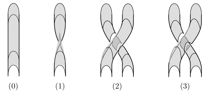
Figure 8. A diagram $D_{A,t}$ consists of one of (1), (2), (3), or their inverses and some copies of (0) ($t=1,\ldots,c$).

Let $s$, $l$, $a$, and $f$ be the numbers of semi-sheets (or semi-arcs) of $D_{S}$, $D_{L}$, $D_{A}$, and $D_{F}$, respectively. We denote semi-sheets (or semi-arcs) of $D_{S}$, $D_{L}$, $D_{A}$, and $D_{F}$ by $x_{1},\ldots,x_{s}$, $y_{1},\ldots,y_{l}$, $z_{1},\ldots,z_{a}$, and $w_{1},\ldots w_{f}$, respectively. Since $S$ is a braided surface, a semi-sheet of $D_{S}$ containing $\pi(q_{i},y_{0})$ is different from a semi-sheet of $D_{S}$ containing $\pi(q_{j},y_{0})$ for any $i\neq j$. This is true for $D_{L}$ and $D_{A}$. Hence, by replacing subscripts of semi-sheets and semi-arcs, we assume that

• for $h=1,\ldots,2m$, a semi-sheet $x_{h}$ contains $\pi(q_{i},y_{0})$,

• for $i=1,\ldots,2m$, a semi-arc $y_{i}$ contains $\pi(q_{i},y_{0})$, and

• for $j=1,\ldots,m$, a semi-sheet $z_{j}$ contains $\pi(q_{2i},y_{0})$ and $\pi(q_{2i-1},y_{0})$.

We give semi-sheets of $D_{A}$ and $D_{F}$ orientations arbitrarily. We give semi-sheets of $D_{S}$ the orientation induced from an orientation of $S$ which is compatible with an orientation of $D_{2}$. We also give semi-arcs of $D_{L}$ the orientation induced from semi-sheets of $D_{S}$.

Remark 4.5.

The significance of giving such orientations is that for each wicket $w$ that forms $A_{S}$, the orientations of semi-sheets of $D_{S}$ containing endpoints of $w$ are incoherent across $w$.

For each semi-arc $y_{i}$, there are unique semi-sheets $x_{h}$, $z_{j}$, and $w_{k}$ such that $y_{i}\subset x_{h}$, $y_{i}\subset z_{j}$, and $y_{i}\subset w_{k}$, respectively. We denote $h(y_{i})=h$, $j(y_{i})=j$ and $k(y_{i})=k$. Similarly, for each semi-sheet $x_{h}$ (and $y_{i}$), there is a unique semi-sheet $w_{k}$ such that $x_{h}\subset w_{k}$ (and $y_{i}\subset w_{k}$), respectively. We denote $k(x_{h})=k$ and $k(y_{i})=k$.

For each semi-sheet $x_{h}$, we define the sign $\varepsilon_{h}=1$ if the orientation of $x_{h}$ is coherent with the orientation of $w_{k(x_{h})}$ under the natural inclusion $x_{h}\subset w_{h(x_{h})}$ and $\varepsilon_{h}=-1$ otherwise. Similarly, for each semi-arc $y_{i}$ (and semi-sheet $z_{j}$), we define the signs $\zeta_{i}=1$ (and $\eta_{j}=1$) if the orientations of $x_{h(y_{i})}$ (and $z_{j}$) are coherent with the orientations of $w_{k(y_{i})}$ (and $w_{k(z_{j})}$) under the natural inclusions $x_{h(y_{i})}\subset w_{k(y_{i})}$ (and $z_{j}\subset w_{k(z_{j})}$) and $\zeta_{i}=-1$ (and $\eta_{j}=-1$) otherwise, respectively.

We denote $X_{h}=x_{h}^{\varepsilon_{h}}$, $Y_{i}=y_{i}^{\zeta_{i}}$, and $Z_{j}=z_{j}^{\eta_{j}}$, and put

$$R_{1}^{X}~{}=~{}\{Y_{i}=X_{h(y_{i})}~{}|~{}i=1,\ldots,l~{}\}\quad\mbox{and}\quad R_{1}^{Z}=\{Y_{i}=Z_{j(y_{i})}~{}|~{}i=1,\ldots,l~{}\}.$$

Lemma 4.6.

$X(F)$ has the following presentation:

(4.3) $$\left\langle\begin{array}[]{c|}x_{1},\ldots,x_{s},~{}y_{1},\ldots,y_{l},~{}z_{1},\ldots,z_{a}\end{array}\begin{array}[]{c}\mbox{A-rel}_{D_{S}},\mbox{B-rel}_{D_{S}},R_{1}^{X},R_{1}^{Z}\end{array}\right\rangle_{\mathrm{sq}}.$$

Here, each generators $x_{h}$, $y_{i}$, and $z_{j}$ in (4.3) are the images of $x_{h}\in X(S)$, $y_{i}\in X(L)$, and $z_{j}\in X(A)$ by the homomorphisms induced from the inclusion maps, respectively.

Proof.

From Proposition 4.2, $X(F)$ has the following presentation:

(4.6) $$X(F)~{}=~{}\left\langle\begin{array}[]{c}w_{1},\ldots,w_{f}\end{array}\begin{array}[]{|c}\mbox{A-rel}_{D_{F}},\mbox{B-rel}_{D_{F}}\end{array}\right\rangle_{\mathrm{sq}}.$$

We put $R_{0}^{X}=\{w_{k(x_{h})}=X_{h}~{}|~{}h=1,\ldots,s\}$ and $R_{0}^{Z}=\{w_{k(z_{j})}=Z_{j}~{}|~{}j=1,\ldots,a\}$. We add new generators $x_{1},\ldots,x_{s}$, $z_{1},\ldots,z_{a}$, and $y_{1},\ldots,y_{l}$ with $R_{0}^{X}$, $R_{0}^{Z}$, and $R_{1}^{Z}$ to (4.6):

(4.10) $$X(F)~{}=~{}\left\langle\begin{array}[]{c|}x_{1},\ldots,x_{s},~{}y_{1},\ldots,y_{l},\\ z_{1},\ldots,z_{a},~{}w_{1},\ldots w_{f}\end{array}\begin{array}[]{c}\mbox{A-rel}_{D_{F}},\mbox{B-rel}_{D_{F}},R_{0}^{X},R_{0}^{Z},R_{1}^{Z}\end{array}\right\rangle_{\mathrm{sq}}.$$

Each double point stratum of $D_{S}$ is contained in one of $D_{F}$. Hence A-relations (and B-relations) for $D_{S}$ are consequences of an A-relation (and B-relation) for $D_{F}$ and relators in $R_{0}^{X}$, respectively. Conversely, it follows from Lemma 4.4 that every double point stratum of $D_{F}$ contains one of $D_{S}$. This implies that A-relations (and B-relation) for $D_{F}$ is a consequence of A-relations (and B-relation) for $D_{S}$ and relations in $R_{0}^{X}$. Thus, we replace $\mbox{A-rel}_{D_{F}}$ and $\mbox{B-rel}_{D_{F}}$ in (4.10) with $\mbox{A-rel}_{D_{S}}$ and $\mbox{B-rel}_{D_{S}}$:

(4.14) $$X(F)~{}=~{}\left\langle\begin{array}[]{c|}x_{1},\ldots,x_{s},~{}y_{1},\ldots,y_{l},\\ z_{1},\ldots,z_{a},~{}w_{1},\ldots w_{f}\end{array}\begin{array}[]{c}\mbox{A-rel}_{D_{S}},\mbox{B-rel}_{D_{S}},R_{0}^{X},R_{0}^{Z},R_{1}^{Z}\end{array}\right\rangle_{\mathrm{sq}}.$$

Since $R_{1}^{X}$ consists of consequences of relators in (4.14), we add $R_{1}^{X}$ to (4.14):

(4.18) $$X(F)~{}=~{}\left\langle\begin{array}[]{c|}x_{1},\ldots,x_{s},~{}y_{1},\ldots,y_{l},\\ z_{1},\ldots,z_{a},~{}w_{1},\ldots,w_{f}\end{array}\begin{array}[]{c}\mbox{A-rel}_{D_{S}},\mbox{B-rel}_{D_{S}}.R_{0}^{X},R_{0}^{Z},R_{1}^{X},R_{1}^{Z}\end{array}\right\rangle_{\mathrm{sq}}.$$

By Lemma 4.4, each semi-sheet $w_{k}$ contains some semi-sheet $x_{h}$ of $D_{S}$. Hence there exists a relator $w_{k(x_{h})}=X_{h}$ in $R_{0}^{X}$ such that $k(x_{h})=k$. We fix such a relator for each $w_{k}$ and denote it as $r(w_{k})$. Let $R_{0}^{W}=\{r(w_{k})~{}|~{}k=1,\ldots,f\}$.

Let $w_{k(x_{h})}=X_{h}$ be a relator in $R_{0}^{X}\setminus R_{0}^{W}$. We will show that $w_{k(x_{h})}=X_{h}$ is a consequence of $R_{0}^{W}$, $R_{1}^{X}$, and $R_{1}^{Z}$. By definition, there is a relator $w_{k}=X_{h_{0}}$ in $R_{0}^{W}$ such that $k(x_{h})=k$. Let $p:[0,1]\to w_{k}$ be a path on the semi-sheet $w_{k}$ such that endpoints $p(0)$ and $p(1)$ are on semi-sheets $x_{h_{0}}$ and $x_{h}$, respectively. We may assume that the image of $p$ intersects with semi-arcs $y_{i_{1}},\ldots,y_{i_{2q}}$ of $D_{L}$ transversely on $w_{k}$, see Figure 9. For $u=1,\ldots,q$, we denote $h_{u}=h(y_{i_{2u}})$ and $j_{u}=j(y_{i_{2u}})$. Then, $Y_{i_{2u}}=X_{h_{u}}$ and $Y_{i_{2u-1}}=X_{h_{u-1}}$ are relators in $R_{1}^{X}$, and $Y_{i_{2u}}=Z_{j_{u}}$ and $Y_{i_{2u-1}}=Z_{j_{u}}$ are relators in $R_{1}^{Z}$. Hence $Y_{i_{1}}=Y_{i_{2q}}$ is a consequences of $R_{1}^{X}$ and $R_{1}^{Z}$. Since $w_{k}=X_{h_{0}}$, $Y_{i_{1}}=X_{h_{0}}$, and $Y_{i_{2q}}=X_{h}$ are relators in $R_{0}^{W}$, $R_{1}^{X}$, and $R_{1}^{Z}$, respectively, $w_{k(x_{h})}=X_{h}$ is a consequence of them.

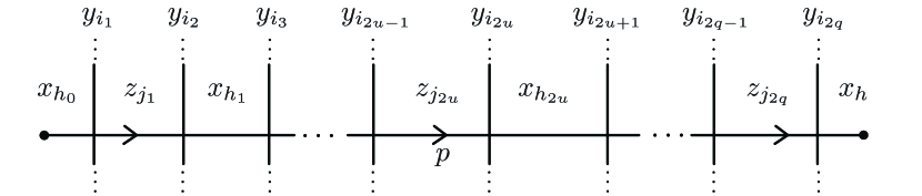
Figure 9. An illustration of intersections of the image of $p$ and semi-arcs of $D_{L}$ on the semi-sheet $w_{k}$.

Similarly, every relator in $R_{0}^{Z}$ is a consequence of $R_{0}^{W}$, $R_{1}^{X}$, and $R_{1}^{Z}$. Thus, we remove $R_{0}^{X}\setminus R_{0}^{W}$ and $R_{0}^{Z}$ from (4.18):

(4.22) $$X(F)~{}=~{}\left\langle\begin{array}[]{c|}x_{1},\ldots,x_{s},~{}y_{1},\ldots,y_{l},\\ z_{1},\ldots,z_{a},~{}w_{1},\ldots,w_{f}\end{array}\begin{array}[]{c}\mbox{A-rel}_{D_{S}},\mbox{B-rel}_{D_{S}},R_{0}^{W},R_{1}^{X},R_{1}^{Z}\end{array}\right\rangle_{\mathrm{sq}}.$$

Then generators $w_{1},\ldots,w_{f}$ do not occur in relators in (4.22) except for $R_{0}^{W}$ so that we remove $w_{1},\ldots,w_{f}$ and $R_{0}^{W}$ from (4.22). Hence we obtain (4.3). ∎

Next, we define a subset $R_{2}$ of $R_{1}^{Z}$. Let $Q=\{Y_{2j-1}=Z_{j},Y_{2j}=Z_{j}~{}|~{}j=1,\ldots,m\}$ be a subset of $R_{1}^{Z}$. If $m=a$, we simply define $R_{2}=R_{1}^{Z}=Q$, where $m$ is the half of the degree of $S$. If $m<a$, we need to fix a relator $r_{j}:Y_{i}=Z_{j}$ in $R_{1}^{Z}$ for $j=m+1,\ldots,a$ as follows:

Let $t(y_{i})$ (and $t(z_{j})$) be the minimum numbers of second subscripts of diagrams $D_{A,t}$ which intersect with $y_{i}$ (and $z_{j}$) in $D_{A}$, respectively. Clearly, $t(y_{i})\geq t(z_{j(y_{i})})$ holds for any $i$. In addition, for $j=1,\ldots,a$, there exists a semi-sheet $y_{i}$ such that $t(y_{i})=t(z_{j})$. For $j=1,\ldots,a$ and $t=1,\ldots,c$, we put

$$R_{1}^{t}~{} =~{}\{Y_{i}=Z_{j(y_{i})}~{}|~{}t(i)=t~{}(i=1,\ldots,l)\},~{}\mbox{and}$$

$$R_{1}^{t,j}~{} =~{}\{Y_{i}=Z_{j(y_{i})}~{}|~{}t(i)=t,~{}j(y_{i})=j~{}(i=1,\ldots,l)\}.$$

Here, a relator $Y_{i}=Z_{k}$ belonging to $R_{1}^{t}$ ($t\geq 1$) indicates that the semi-arc $y_{i}$ intersects with $D_{A,t}$ and does not intersect with $D_{A,1},\ldots,D_{A,t-1}$. By definition, $R_{1}^{t,j}$ is the empty set for any $t<t(z_{j})$, and $R_{1}^{t(z_{j}),j}$ is a non-empty set. For each $j=m+1,\ldots,a$, we fix a relator $r_{j}\in R_{1}^{t(z_{j}),j}$, and we define

$$R_{2}=Q~{}\cup~{}\left\{r_{m+1},r_{m+2},\ldots,r_{a}\right\}.$$

Lemma 4.7.

$X(F)$ has the following presentation:

(4.25) $$\left\langle\begin{array}[]{c|}x_{1},\ldots,x_{s},~{}y_{1},\ldots,y_{l},~{}z_{1},\ldots,z_{a}\end{array}\begin{array}[]{l}\mbox{A-rel}_{D_{S}},\mbox{B-rel}_{D_{S}},R_{1}^{X},R_{2}\end{array}\right\rangle_{\mathrm{sq}}.$$

Proof.

We will show that relators in $R_{1}^{Z}\setminus R_{2}$ are consequences of relators in (4.25). Since A-relations (and B-relations) for semi-arcs of $D_{L}$ are consequences of relators in $\mbox{A-rel}_{D_{S}}$ (and $\mbox{B-rel}_{D_{S}}$) and $R_{1}^{X}$, respectively, we use relators in $\mbox{A-rel}_{D_{L}}$ and $\mbox{B-rel}_{D_{L}}$ instead of $\mbox{A-rel}_{D_{S}}$ and $\mbox{B-rel}_{D_{S}}$ in the following argument.

$R_{1}^{Z}$ is divided into $c$ subsets $R_{1}^{1},R_{1}^{2},\ldots,R_{1}^{c}$. Thus, it suffices to show that relators in $R_{1}^{t}\setminus(R_{2}\cap R_{1}^{t})$ are consequences of relators in (4.25). We will show this by induction on $t$. We put $R_{2}^{0}=R_{2}$ and $R_{2}^{t}=R_{2}\cap(\bigcup_{s=1}^{t}R_{1}^{s})$ for $t\geq 1$. Then, $R_{2}^{t-1}$ consists of consequences of relators in (4.25) obtained from the assumption of induction at $t$. Since the arguments for the case when $t=1$ and the case when $t\geq 2$ are parallel, we will discuss both cases simultaneously in the following.

The diagram $D_{A,t}$ is a disjoint union of one of Figure 8-(1), -(2), -(3), or their inverses and some copies of Figure 8-(0). If a semi-arc $y_{i}$ intersects with a copy of Figure 8-(0) in $D_{A,t}$, then it holds that $t(y_{i})<t$ and $t(z_{j(y_{i})})<t$. Thus $Y_{i}=Z_{j(y_{i})}$ belongs to $R_{2}^{t-1}$. Hence we consider a relator $Y_{i}=Z_{j(y_{i})}$ in $R_{1}^{Z}$ such that $y_{i}$ intersects with one of Figure 8-(1), -(2), -(3), or their inverses in $D_{A,t}$.

(1) We first consider the case $\gamma_{t}=\sigma_{2k-1}$ ($k=1,\ldots,m$), that is, $D_{A,t}$ contains a subdiagram as shown in the center of Figure 10. The right of Figure 10 is shown semi-sheets of its subdiagram. It holds that $1\leq j_{1}\leq m$ when $t=1$. For $t\geq 2$, the semi-sheet $z_{j_{1}}$ intersects with $D_{A,t-1}$, i.e., $t(z_{j_{1}})<t$. The semi-sheet $z_{j_{2}}$ might be satisfied $1\leq j_{2}\leq m$. In such a case, $R_{1}^{t}\setminus(R_{2}\cap R_{1}^{t})$ is the empty set. Thus we exclude such a case and assume that $j_{2}$ is more than $m$, which implies $t(z_{j_{2}})=t$ and $t(y_{i_{3}})=t(y_{i_{4}})=t$. Hence we have

$$R_{1}^{t,j_{1}}~{} =~{}\left\{\begin{array}[]{ll}\{Y_{i_{1}}=Z_{j_{1}},Y_{i_{2}}=Z_{j_{1}}\}&(t=1),\\ \emptyset&(t\geq 2),\end{array}\right.$$

$$R_{1}^{t,j_{2}}~{} =~{}\{Y_{i_{3}}=Z_{j_{2}},Y_{i_{4}}=Z_{j_{2}}\}\quad(t\geq 1),$$

$$R_{1}^{t}~{} =~{}\left\{\begin{array}[]{ll}Q~{}\cup~{}R_{1}^{t,j_{2}}&(t=1),\\ R_{1}^{t,j_{2}}&(t\geq 2).\end{array}\right.$$

$$R_{2}\cap R_{1}^{t}~{} =~{}\left\{\begin{array}[]{ll}Q~{}\cup~{}\left\{r_{j_{2}}\right\}&(t=1),\\ \left\{r_{j_{2}}\right\}&(t\geq 2),\end{array}\right.$$

where $r_{j_{2}}\in R_{2}$ is a fixed relator in $R_{1}^{t,j_{2}}$. Thus $R_{1}^{t}\setminus(R_{2}\cap R_{1}^{t})$ consists of one relator, and such a relator, denoted by $\overline{r_{j_{2}}}$, comes from $R_{1}^{t,j_{2}}$.

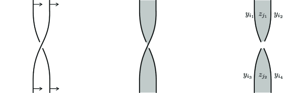
Figure 10. A diagram of a part of $\sigma_{2k-1}$ with normal orientations (left), a diagram of a part of $A_{t}$ (center), and semi-sheets of a part of $A_{t}$ (right).

Then, we can compute that $Y_{i_{3}}=Y_{i_{4}}$ is a consequence of relators in $\mbox{A-rel}_{D_{L}}$, $\mbox{B-rel}_{D_{L}}$, and $R_{2}^{t-1}$:

(4.26) $$\begin{split}Y_{i_{4}}~{}=~{}y_{i_{4}}^{\zeta_{i_{4}}}~{}\stackrel{{\scriptstyle B}}{{=}}~{}(y_{i_{1}}^{y_{i_{2}}})^{\zeta_{i_{4}}}~{}\stackrel{{\scriptstyle(*)}}{{=}}~{}(y_{i_{1}})^{\zeta_{i_{4}}}~{}\stackrel{{\scriptstyle R}}{{=}}~{}Z_{j_{1}}^{\zeta_{i_{1}}\zeta_{i_{4}}}~{}\stackrel{{\scriptstyle R}}{{=}}~{}y_{i_{2}}^{\zeta_{i_{2}}\zeta_{i_{1}}\zeta_{i_{4}}}~{}\stackrel{{\scriptstyle}}{{=}}~{}y_{i_{2}}^{-\zeta_{i_{4}}}~{}\stackrel{{\scriptstyle A}}{{=}}~{}y_{i_{3}}^{-\zeta_{i_{4}}}~{}\stackrel{{\scriptstyle}}{{=}}~{}y_{i_{3}}^{\zeta_{i_{3}}}~{}=~{}Y_{i_{3}}.\end{split}$$

Here, two elements are connected by $\stackrel{{\scriptstyle A}}{{=}}$, $\stackrel{{\scriptstyle B}}{{=}}$, and $\stackrel{{\scriptstyle R}}{{=}}$ if the equality is given from a relator in $\mbox{A-rel}_{D_{L}}$, $\mbox{B-rel}_{D_{L}}$, and $R_{2}^{t-1}$, respectively. The equality expressed by ($*$) is obtained from a result of $y_{i_{2}}=z_{j_{1}}^{\eta_{j_{1}}\zeta_{i_{2}}}=y_{i_{1}}^{\zeta_{i_{1}}\zeta_{i_{2}}}=y_{i_{1}}^{-1}$. Hence, $\overline{r_{j_{2}}}$ is a consequence of $r_{j_{2}}$ and $Y_{i_{3}}=Y_{i_{4}}$, that is, $R_{1}^{t}\setminus(R_{2}\cap R_{1}^{t})$ consists of a consequence of relators in (4.25). Similarly, we can prove it in the case of $\gamma_{t}=\sigma_{2k-1}^{-1}$.

(2) Next, we consider the case $\gamma_{t}=\tau_{k}$ ($k=1,\ldots,m-1$), that is, $D_{A,t}$ contains a subdiagram as in the center of Figure 11. The right of Figure 11 is shown semi-sheets of the subdiagram.

It holds that $1\leq j_{1}\leq m$ and $1\leq j_{4}\leq m$ when $t=1$. For $t\geq 2$, $t(y_{i_{1}}),t(y_{i_{2}}),t(y_{i_{7}})$, and $t(t_{i_{8}})$ are less than $t$. For $t\geq 1$, $j_{2}$, $j_{5}$, and $j_{6}$ are more than $m$. For a similar reason as in (1), we may assume that $j_{3}$ is also more than $m$ for $t\geq 1$ and that $j_{4}$ is also more than $m$ for $t\geq 2$. Then, we have

(4.27) $$\begin{split}R_{1}^{t,j_{1}}~{}&=~{}\left\{\begin{array}[]{ll}\{Y_{i_{1}}=Z_{j_{1}},Y_{i_{2}}=Z_{j_{1}}\}&(t=1),\\ \emptyset&(t\geq 2),\end{array}\right.\\ R_{1}^{t,j_{2}}~{}&=~{}\{Y_{i_{3}}=Z_{j_{2}},Y_{i_{4}}=Z_{j_{2}}\},\quad\,R_{1}^{t,j_{3}}~{}=~{}\{Y_{i_{5}}=Z_{j_{3}},Y_{i_{6}}=Z_{j_{3}}\},\quad(t\geq 1)\\ R_{1}^{t,j_{4}}~{}&=~{}\left\{\begin{array}[]{ll}\{Y_{i_{11}}=Z_{j_{4}},Y_{i_{12}}=Z_{j_{4}},Y_{i_{7}}=Z_{j_{4}},Y_{i_{8}}=Z_{j_{4}}\}&(t=1),\\ \{Y_{i_{11}}=Z_{j_{4}},Y_{i_{12}}=Z_{j_{4}}\}&(t\geq 2),\end{array}\right.\\ R_{1}^{t,j_{5}}~{}&=~{}\{Y_{i_{9}}=Z_{j_{5}}\},\quad R_{1}^{t,j_{6}}~{}=~{}\{Y_{i_{10}}=Z_{j_{6}}\}\quad(t\geq 1),\\ R_{1}^{t}~{}&=~{}\left\{\begin{array}[]{ll}Q\cup R_{1}^{t,j_{1}}\cup\cdots\cup R_{1}^{t,j_{6}}&(t=1),\\ R_{1}^{t,j_{1}}\cup\cdots\cup R_{1}^{t,j_{6}}&(t\geq 2),\end{array}\right.\\ R_{2}\cap R_{1}^{t}~{}&=~{}\left\{\begin{array}[]{ll}Q\cup\{r_{j_{2}},r_{j_{3}},Y_{i_{9}}=Z_{j_{5}},Y_{i_{10}}=Z_{j_{6}}\}&(t=1),\\ \{r_{j_{2}},r_{j_{3}},Y_{i_{9}}=Z_{j_{5}},Y_{i_{10}}=Z_{j_{6}}\}&(t\geq 2).\end{array}\right.\end{split}$$

Let $\overline{r_{j_{2}}}$ and $\overline{r_{j_{3}}}$ be relators in $R_{1}^{t,j_{2}}$ and $R_{1}^{t,j_{3}}$ which are not $r_{j_{2}}$ and $r_{j_{3}}$, respectively. Then, $R_{1}^{t}\setminus(R_{2}\cap R_{1}^{t})$ consists of four relators, which are $Y_{i_{11}}=Z_{j_{4}}$, $Y_{i_{12}}=Z_{j_{4}}$, $\overline{r_{j_{2}}}$, and $\overline{r_{j_{3}}}$.

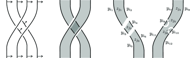
Figure 11. A diagram of a part of $\tau_{k}$ with normal orientations (left), a diagram of a part of $A_{1}$ (center), and semi-sheets of a part of $A_{t}$ (right).

By similar computations as shown in (4.26), both $Y_{i_{3}}=Y_{i_{4}}$ and $Y_{i_{5}}=Y_{i_{6}}$ are consequences of relators in (4.25). Hence, $\overline{r_{j_{2}}}$ and $\overline{r_{j_{3}}}$ are also consequences of them. By the following computations, $Y_{i_{11}}=Z_{j_{4}}$ and $Y_{i_{12}}=Z_{j_{4}}$ are also consequences of them:

$$Y_{i_{11}}~{}\stackrel{{\scriptstyle A}}{{=}}~{}Y_{i_{9}}~{}\stackrel{{\scriptstyle A}}{{=}}~{}Y_{i_{7}}~{}\stackrel{{\scriptstyle R}}{{=}}~{}Z_{j_{4}},\quad Y_{i_{12}}~{}\stackrel{{\scriptstyle A}}{{=}}~{}Y_{i_{10}}~{}\stackrel{{\scriptstyle A}}{{=}}~{}Y_{i_{8}}~{}\stackrel{{\scriptstyle R}}{{=}}~{}Z_{j_{4}}.$$

Therefore, we see that all elements of $R_{1}^{t}\setminus(R_{2}\cap R_{1}^{t})$ are consequences of (4.25). This computation can be applied to the case $\gamma_{t}=\tau_{k}^{-1}$.

(3) Finally, we consider the case $\gamma_{t}=\upsilon_{k}$ ($k=1,\ldots,m$), that is, $D_{A,t}$ contains a subdiagram as in the center of Figure 12.

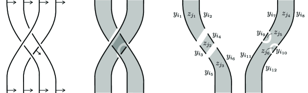
Figure 12. A diagram of a part of $\upsilon_{k}$ with normal orientations (left), a diagram of a part of $A_{t}$ (center), and semi-sheets of a part of $A_{t}$ (right).

Since semi-sheets are same for the case (2), $R_{1}^{t}$ and $R_{2}\cap R_{1}^{t}$ are the same as (4.27). Hence we can see that $R_{1}^{t}\setminus R_{1}$ consists of four elements and that these relators are consequences of relators in (4.25). This computation can be applied when $\gamma_{t}=\upsilon_{k}^{-1}$.

Therefore, we remove relators in $R_{1}^{Z}\setminus R_{2}$ from (4.3), and obtain (4.25). ∎

Proof of Theorem 1.1.

By Tietze moves (T4), we remove generators $z_{m+1},\ldots,z_{a}$ and relators $r_{m+1},\ldots,r_{a}\in R_{2}$ from (4.25):

$$X(F)~{}=~{}\left\langle\begin{array}[]{c}x_{1},\ldots,x_{s},~{}y_{1},\ldots,y_{l},~{}z_{1},\ldots,z_{m}\end{array}\begin{array}[]{|c}\mbox{A-rel}_{D_{S}},\mbox{B-rel}_{D_{S}},R_{1}^{X},Q\end{array}\right\rangle_{\mathrm{sq}},$$

where $R_{1}^{X}=\{X_{h(y_{i})}=Y_{i}~{}|~{}1\leq i\leq l\}$ and $Q=\{Y_{2k}=Z_{k},Y_{2k-1}=Z_{k}~{}|~{}1\leq k\leq m\}$.

We put $R_{3}=\{Y_{2k}=Z_{k}~{}|~{}1\leq k\leq m\}$ and $R_{4}=\{X_{2k-1}=X_{2k}~{}|~{}1\leq k\leq m\}$. Since $h(y_{2k})=h(y_{2k-1})=k$ for $k=1,\ldots,2m$, relators in $R_{3}$ and $R_{4}$ are consequences of $R_{1}^{X}$ and $Q$. Conversely, relators in $Q$ are consequences of $R_{1}^{X}$, $R_{3}$, and $R_{4}$. Thus, we replace $Q$ with $R_{3}$ and $R_{4}$. Furthermore, we remove generators $z_{1},\ldots,z_{m}$ and $y_{1},\ldots,y_{l}$ with $R_{3}$ and $R_{1}^{X}$:

$$X(F)~{}=~{}\left\langle\begin{array}[]{c}x_{1},\ldots,x_{s}\end{array}\begin{array}[]{|c}\mbox{A-rel}_{D_{S}},\mbox{B-rel}_{D_{S}},R_{4}\end{array}\right\rangle_{\mathrm{sq}}.$$

By Remark 4.5, $\varepsilon_{2k}=-\varepsilon_{2k-1}$ holds for $k=1,\ldots,m$. Hence $R_{4}$ can be rewritten as

(4.31) $$X(F)~{}=~{}\left\langle\begin{array}[]{c}x_{1},\ldots,x_{s}\end{array}\begin{array}[]{|c}\mbox{A-rel}_{D_{S}},\mbox{B-rel}_{D_{S}},\\ x_{2k}=x_{2k-1}^{-1}~{}(k=1,\ldots,m)\end{array}\right\rangle_{\mathrm{sq}}.$$

Thus we obtain Theorem 1.1 from (4.31) by applying Propositions 4.2 and 4.3. ∎

Remark 4.8.

Since the knot group $G(F)=\pi_{1}(\mathbb{R}^{4}\setminus N(F))$ of $F$ is isomorphic to the associated group of the knot symmetric quandle of $F$ ([10]), Theorem 1.1 induces a group presentation of $G(F)$:

$$G(F)~{}\cong~{}\left\langle x_{1},\ldots,x_{2m}~{}\begin{array}[]{|c}\mathrm{Artin}(\beta_{j})(x_{k_{i}})=\mathrm{Artin}(\beta_{j})(x_{k_{i}+1})~{}(i=1,\ldots,r)\\ x_{2k-1}=x_{2k}^{-1}~{}(k=1,\ldots,m)\end{array}\right\rangle_{\mathrm{grp}},$$

where $\mathrm{Artin}:B_{m}\to\mathop{\mathrm{Aut}}\nolimits(F_{2m})$ is Artin’s braid automorphism (cf. [8]).

5. Proofs of Theorems 1.2 and 1.3

In this section, we give proofs of Theorems 1.2 and 1.3. The key concept behind the following proof of Theorem 1.2 is based on [18, Lemma 2.7].

Proof of Theorem 1.2.

Let $F$ be a surface-link and $X$ be a finite symmetric quandle. Since $\mathrm{col}_{X}(F)$ is defined as the cardinal number of (symmetric quandle) homomorphisms from $X(F)$ to $X$, it suffices to show the inequality

$$\#\mathrm{Hom}(X(F),X)\leq(\#X)^{\mbox{Plat}(F)}.$$

Let $S$ be an adequate braided surface of degree $2m$ such that $\widetilde{S}\cong F$ and $m=\mathrm{Plat}(F)$. By Theorem 1.1, the knot symmetric quandle $X(F)$ has a presentation with $2m$ generators $x_{1},\ldots,x_{2m}$. We can remove a generator $x_{2j-1}$ with a relator $x_{2j}=x_{2j-1}^{-1}$ from the presentation ($j=1,\ldots,m$). Thus the knot symmetric quandle $X(F)$ is generated by $m$ elements. Since a homomorphism is determined by the images of generators of the domain quandle, $\#\mathrm{Hom}(X(F),X)$ is less than or equal to $(\#X)^{m}$, i.e., we have the inequality. ∎

Proof of Theorem 1.3.

First, for an integer $m\geq 2$ and a prime number $p\geq 3$, we construct a 2-knot $F(m,p)$ as follows: Let $b(m,p)$ be a $(2m-2)$-tuple of $2m$-braids defined as

$$b(m,p)~{}=~{}(\beta^{-1}\sigma_{1}\beta,~{}\beta^{-1}\sigma_{1}^{-1}\beta,~{}\beta^{-1}\sigma_{3}\beta,~{}\beta^{-1}\sigma_{3}^{-1}\beta,~{}\ldots,~{}\beta^{-1}\sigma_{2m-3}\beta,~{}\beta^{-1}\sigma_{2m-3}^{-1}\beta),$$

where $\beta=(\sigma_{2}\sigma_{4}\cdots\sigma_{2m-2})^{p}\in B_{2m}$. Then, $b(m,p)$ is a braid system for a $2$-dimensional braid $S(m,p)$ of degree $2m$. Let $F(m,p)$ be the plat closure of $S(m,p)$. By definition, we have the inequality $\mathrm{Plat}(F(m,p))\leq\mathrm{g.Plat}(F(m,p))\leq m$. Furthermore, $F(m,p)$ is a 2-knot because $F(m,p)$ is connected and $\chi(F(m,p))=m-(2m-2)+m=2$.

By Theorem 1.1, the knot symmetric quandle $X(F)$ has the following presentation:

(5.3) $$X(F)~{}=~{}\left\langle x_{1},\ldots,x_{2m}~{}\begin{array}[]{|cl}\mathrm{Artin}(\beta)(x_{2i-1})=\mathrm{Artin}(\beta)(x_{2i}){}&(i=1,\ldots,m-1)\\ x_{2j-1}=\rho(x_{2j})&(j=1,\ldots,m)\end{array}\right\rangle_{\mathrm{sq}}.$$

Let $q\geq 3$ be a prime number and $(R_{q},\mathop{\mathrm{id}}\nolimits)$ be the symmetric dihedral quandle of order $q$. Let $f:A=\{x_{1},\ldots,x_{2m}\}\to R_{q}$ be a map and $f_{\sharp}:\mbox{FSQ}(A)\to R_{q}$ be a homomorphism induced from $f$. We write $y_{i}=f_{\sharp}(x_{i})$. Since $\beta=(\sigma_{2}\sigma_{4}\cdots\sigma_{2m-2})^{p}$, we have

$$f_{\sharp}(\mathrm{Artin}(\beta)(x_{k}))~{}=~{}\begin{cases}y_{1}&(k=1),\\ py_{2k+1}-(p-1)y_{2k}&(k=2,4,\ldots,2m-2),\\ (p+1)y_{2k-2}-py_{2k-1}&(k=3,5,\ldots,2m-1),\\ y_{2m}&(k=2m).\end{cases}$$

By Lemma 3.8, $f$ extends to a homomorphism $f:X(F(m,p))\to R_{q}$ if and only if the following equations hold:

$$\begin{array}[]{rll}y_{1}&=~{}~{}py_{3}-(p-1)y_{2},&\\ (p+1)y_{2i-1}-py_{2i-2}&=~{}~{}py_{2i+1}-(p-1)y_{2i}&(i=2,\ldots,m-1),\\ y_{2j-1}&=~{}~{}y_{2j}&(j=1,\ldots,m).\end{array}$$

If $p\neq q$, the above equations lead to $y_{1}=y_{2}=\cdots=y_{2m}$. Hence, every symmetric quandle homomorphism is a constant function, i.e., $\mathrm{col}_{(R_{q},\mathop{\mathrm{id}}\nolimits)}(F(m,p))=q$. Since $qy=0$ holds for any $y\in R_{q}$, if $p=q$, then the above equations can be reduced to $y_{2j-1}=y_{2j}$ $(j=1,\ldots,m)$, i.e., $\mathrm{col}_{(R_{q},\mathop{\mathrm{id}}\nolimits)}(F(m,p))=q^{m}$.

By Theorem 1.2, we have $\mathrm{Plat}(F(m,p))=\mathrm{g.Plat}(F(m,p))\geq m$. Thus, the plat index and genuine plat index of $F(m,p)$ are equal to $m$. In addition, for two distinct prime numbers $p,q\geq 3$, the $(R_{p},\mathop{\mathrm{id}}\nolimits)$-coloring number detects that 2-knots $F(m,p)$ and $F(m,q)$ are inequivalent. Hence we obtain infinitely many 2-knots with $\mathrm{Plat}(F(m,p))=\mathrm{g.Plat}(F(m,p))=m$.

Finally, for an integer $g\geq 1$, we construct a surface-knot $F(m,p,g)$ of genus $g$ such that $\mathrm{Plat}(F(m,p,g))=\mathrm{g.Plat}(F(m,p,g))=m$.

Let $b(p,m,g)$ be a $(2m-2+2g)$-tuple of $2m$-braids defined as

$$b(p,m,g)~{}=~{}b(m,p)\oplus(\beta^{-1}\sigma_{1}\beta,\ldots,\beta^{-1}\sigma_{1}\beta)\oplus(\beta^{-1}\sigma_{1}^{-1}\beta,\ldots,\beta^{-1}\sigma_{1}^{-1}\beta),$$

where $\beta=(\sigma_{2}\sigma_{4}\cdots\sigma_{2m-2})^{p}\in B_{2m}$, and the second and third terms are $g$-tuples of $\beta^{-1}\sigma_{1}\beta$’s and $\beta^{-1}\sigma_{1}^{-1}\beta$’s, respectively. Then, $b(p,m,g)$ is a braid system of a $2$-dimensional braid $S(m,p,g)$ of degree $2m$. Let $F(m,p,g)$ be the plat closure of $S(m,p,g)$. Since $F(m,p,g)$ is connected, orientable and $\chi(F(m,p,g))=m-(2m-2+2g)+m=2-2g$, $F(m,p,g)$ is an orientable surface-link of genus $g$.

By Theorem 1.1, the knot symmetric quandle $X(F(m,p,g))$ is isomorphic to $X(F(m,p))$. Hence, the above argument implies that the plat index and the genuine plat index of $F(m,p,g)$ are equal to $m$, and $F(m,p,g)$ and $F(m,q,g)$ are inequivalent if $p\neq q$. ∎

References

- [1] Emil Artin. Theorie der Zöpfe. Abh. Math. Sem. Univ. Hamburg, 4(1):47–72, 1925.
- [2] Joan S. Birman. On the stable equivalence of plat representations of knots and links. Canadian J. Math., 28(2):264–290, 1976.
- [3] Tara Brendle and Allen Hatcher. Configuration spaces of rings and wickets. Commentarii Mathematici Helvetici, 88, 05 2008.
- [4] Roger Fenn and Colin Rourke. Racks and links in codimension two. J. Knot Theory Ramifications, 1(4):343–406, 1992.
- [5] Hugh M. Hilden. Generations for two subgroups of the braid group. Pacific J. Math., 59(2), 1975.
- [6] D. Joyce. A classifying invariants of knots. J. Pure. Appl. Alg., 23:37–65, 1982.
- [7] Seiichi Kamada. Wirtinger presentations for higher dimensional manifold knots obtained from diagrams. Fundamenta Mathematicae - FUND MATH, 168:105–112, 01 2001.
- [8] Seiichi Kamada. Braid and knot theory in dimension four, volume 95 of Mathematical Surveys and Monographs. American Mathematical Society, Providence, RI, 2002.
- [9] Seiichi Kamada. Quandles with good involutions, their homologies and knot invariants. Intelligence of Low Dimensional Topology 2006, pages 101–108, 01 2007.
- [10] Seiichi Kamada. Quandles and symmetric quandles for higher dimensional knots. 103:145–158, 2014.
- [11] Seiichi Kamada. Surface-Knots in -Space. Springer Monographs in Mathematics. Springer, 2017.
- [12] Seiichi Kamada and Kanako Oshiro. Homology groups of symmetric quandles and cocycle invariants of links and surface-links. Trans. Amer. Math. Soc., 362(10):5501–5527, 2010.
- [13] S. Matveev. Distributive groupoids in knot theory. Mat. Sb. (N.S.), 119(161):78–88, 1982.
- [14] B. G. Moishezon. Stable branch curves and braid monodromies. In Anatoly Libgober and Philip Wagreich, editors, Algebraic Geometry, pages 107–192, Berlin, Heidelberg, 1981. Springer Berlin Heidelberg.
- [15] Colin Rourke and Brian Sanderson. Introduction to Piecewise-Linear Topology. Springer Study Edition. Springer, 1982.
- [16] Lee Rudolph. Braided surfaces and Seifert ribbons for closed braids. Comment. Math. Helv., 58(1):1–37, 1983.
- [17] Lee Rudolph. Special positions for surfaces bounded by closed braids. Rev. Mat. Iberoamericana, 1(3):93–133, 1985.
- [18] Kouki Sato and Kokoro Tanaka. The bridge number of surface links and kei colorings. Bull. Lond. Math. Soc., 54(5):1763–1771, 2022.
- [19] O.Ya. Viro. Lecture given at osaka city university. September 1990.
- [20] Jumpei Yasuda. A plat form presentation for surface-links. arXiv:2105.08634, 2021.