Rebalancing Social Feed
to Minimize Polarization and Disagreement

Abstract.

Social media have great potential for enabling public discourse on important societal issues. However, adverse effects, such as polarization and echo chambers, greatly impact the benefits of social media and call for algorithms that mitigate these effects. In this paper, we propose a novel problem formulation aimed at slightly nudging users’ social feeds in order to strike a balance between relevance and diversity, thus mitigating the emergence of polarization, without lowering the quality of the feed. Our approach is based on re-weighting the relative importance of the accounts that a user follows, so as to calibrate the frequency with which the content produced by various accounts is shown to the user.

We analyze the convexity properties of the problem, demonstrating the non-matrix convexity of the objective function and the convexity of the feasible set. To efficiently address the problem, we develop a scalable algorithm based on projected gradient descent. We also prove that our problem statement is a proper generalization of the undirected-case problem so that our method can also be adopted for undirected social networks. As a baseline for comparison in the undirected case, we develop a semidefinite programming approach, which provides the optimal solution. Through extensive experiments on synthetic and real-world datasets, we validate the effectiveness of our approach, which outperforms non-trivial baselines, underscoring its ability to foster healthier and more cohesive online communities.

1. Introduction

The phenomenon of polarization in social-media platforms indicates the emergence of two (or more) distinct poles of opinions, often coupled with structural network segregation (Tucker et al., 2018). In fact, users of these platforms, tend to “follow” other users whose interests and opinions align with their own, both because of natural homophily and because of who-to-follow recommender systems. Moreover, the algorithmically-curated “feed” exposed to each user ends up being constituted largely by content aligned with their own opinion. As a result, algorithms employed by social-media platforms may lead to the well-known “echo-chamber” effect (Quattrociocchi et al., 2016; Cinus et al., 2022), where individuals of similar mindsets reinforce their beliefs while remaining shielded from dissenting viewpoints, thus becoming more polarized (Nikolov et al., 2015; Pariser, 2011).

Addressing the phenomenon of polarization and its negative consequences is crucial for fostering healthy online discourse and mitigating the spread of misinformation and extremism. Various strategies have been proposed to mitigate polarization in social networks (Hartman et al., 2022), including who-to-follow recommendations aimed at minimizing controversy (Garimella et al., 2018), or allocating seed users to optimize various diversity measures (Aslay et al., 2018; Garimella et al., 2017; Tu et al., 2020). However, directly targeting and minimizing polarization can be problematic, as it may infringe upon users’ freedom of expression and foster opposite effects (Bail et al., 2018). Moreover, recommending content or users to follow with a different mindset, might reduce the relevance of the content for the users, potentially eroding their experience on the platform.

In this paper, we study the problem of rebalancing the feed of users in a social network with the aim of minimizing the polarization and disagreement in the network. Our objective is inspired by the work of Musco et al. (2018), but we introduce a novel extension that poses significant challenges, while being more realistic. In more detail, we consider the setting of a directed social network, where a link $(i,j)$ represents a follower-followee relation, and thus user $j$ can influence user $i$. We assume that opinions in the network are formed according to the Friedkin-Johnsen opinion-dynamics model (Friedkin and Johnsen, 1990). Our goal is to re-weight the relative importance of the accounts that a user follows, so as to calibrate the frequency with which the content produced by various accounts is shown to the user. Our approach, by re-balancing the weight of existing links, preserves the total engagement of each user in the social network.

We formally characterize our problem, showing that the objective function is not matrix-convex, but the feasible set is convex. We propose a fast and scalable algorithm based on projected gradient descent, which overcomes the challenges of non-matrix convexity and scalability. We derive a closed-form expression for the gradient with respect to the adjacency matrix, and we exploit its rank-one properties to achieve an efficient evaluation through the Biconjugate Gradient Solver. Furthermore, we outline an efficient projection step and show that our method has approximately linear time complexity in the number of edges of the network.

We also prove that our problem is a proper generalization of the undirected case so that our method can be adopted for undirected graphs. As a baseline for comparison in the undirected case, we also develop a semidefinite programming approach.

We conduct extensive experimentation using both real-world and synthetic datasets, featuring diverse opinion distributions, varying polarization levels, and distinct modularity in the network structure. The results we obtain highlight the superior performance of our method compared to non-trivial baselines, providing empirical evidence of their efficacy in minimizing polarization and disagreement in large real-world social networks.

The key contributions of this paper are as follows:

• We propose a novel problem formulation for re-weighting the links of a directed social network with the goal to minimize polarization and disagreement, under preserving the total engagement for each user (Section 3).

• We rigorously analyze the convexity properties of the problem. Specifically, we prove that the objective function is not matrix-convex while demonstrating the convexity of the feasible set (Section 3). We also show that our problem is a proper generalization of the undirected case.

• For the proposed problem, we develop a projected gradient-descent algorithm that offers scalability and practicality (Section 4.1). In particular, our method has near-linear time complexity in the number of edges per iteration (Section 4.2).

• As a baseline for studying the performance of our method to undirected social networks, we devise a semidefinite programming approach that allows us to obtain an optimal solution for the undirected case (Section 4.3),

• We validate the effectiveness of our approach through a series of extensive experiments conducted on both synthetic and real-world large-scale datasets. We evaluate the performance across a wide range of input instances, providing a comprehensive characterization of its behavior (Section 5).

2. Related Work

The phenomena of bias, polarization, and echo chambers have been studied extensively in social-media research (Vicario et al., 2019; Bessi et al., 2016; Kubin and von Sikorski, 2021). A main challenge has been to develop mitigation strategies (Matakos et al., 2020; Aslay et al., 2018; Interian et al., 2021; Tu et al., 2020; Garimella et al., 2017; Baumann et al., 2023). However, many of the existing methods focus on a static setting, without considering the dynamic nature of the underlying opinion-formation process.

The Friedkin–Johnsen (FJ) opinion-dynamics model (Friedkin and Johnsen, 1990) is the most widely-used framework for studying how opinions form among users in a social network (Acemoglu and Ozdaglar, 2011; Bindel et al., 2015; Xia et al., 2011; Zha et al., 2020). In the FJ model, individuals are represented by nodes in a network and social ties are represented by edges. Individuals update their opinions through an iterative weighted-averaging process that considers their own opinion and the opinions of their neighbors. The model incorporates two key variables: susceptibility and strength of social ties. While some previous research has studied the effects of susceptibility (Abebe et al., 2021; Marumo et al., 2021; Xu et al., 2022), in this paper, we assume that individual susceptibility is inherent to an individual’s personality and, thus, it remains constant. Instead, we focus on structural interventions as a means of shaping opinion dynamics. Structural interventions involve adjusting the weights of social ties, which can be interpreted as ranking scores, or frequencies of posts in users’ social feeds.

The problem of jointly minimizing polarization and disagreement in the FJ model has been studied for undirected graphs in both discrete and continuous cases (Zhu et al., 2021; Musco et al., 2018). Zhu et al. (2021) propose the problem of identifying $k$ new links in an undirected graph to minimize polarization and disagreement. They devise a greedy method to optimize this non-submodular objective function, which provides a constant-factor approximation and runs in cubic time. However, the practical applicability of their approach may be restricted due to its implicit assumptions on the number of link additions.

In the continuous setting, Chen et al. (2018) propose a novel framework for quantifying and optimizing conflict measures in social networks, including polarization, and disagreement. They investigate optimization potential across all sets of prior opinions in average- and worst-case scenarios, addressing challenges in determining globally optimal adjacency matrices using gradient descent. However, their approach focuses on small-graph modifications (deletions, insertions) and does not scale to large networks. Also in the continuous setting, Musco et al. (2018) investigate two problems, both of which differ from the one we study in this paper: the first problem involves optimizing graph topologies, while the second problem aims to optimize initial user opinions.

In the first problem studied by Musco et al. (2018), which is more closely related to our work, the objective is to find a weighted undirected graph that optimizes the objective function, given a total edge-weight budget. However, a key distinction from our formulation is that they do not consider a specific input network. Instead, they explore all possible undirected graph topologies. Consequently, their formulation does not directly translate into actionable solutions such as link recommendation or social-feed curation.

The second key difference with the work of Musco et al. (2018) lies in their focus on undirected graphs. In contrast, our formulation extends to directed (follower-followee) social networks, which are more representative of real-world scenarios. The directed formulation is both more general and more meaningful as, in general, the influence between two users is not symmetric. Furthermore, the non-symmetry of directed graphs poses significant new challenges, stemming from the non-convexity of the objective.

In Section 3.2, we define an undirected version of our problem and demonstrate that the directed version is a proper generalization. This allows our method to be applicable to undirected social networks. Our undirected formulation differs from the problem of Musco et al. (2018) as it considers a given network structure and preserves per-user engagement, instead of distributing a total weight on a discovered graph topology.

In our experiments (Section 5), we compare our method against the SDP (optimal) formulation for undirected instances, which we define in Section 4.3. The SDP formulation can be viewed as a version of the method proposed by Musco et al. (2018), adapted to accommodate a given graph topology. Our results demonstrate that our method outperforms the SDP formulation, as it provides the flexibility to assign different weights to $(i,j)$ and $(j,i)$, while the SDP only produces a symmetrical adjacency matrix.

3. Problem definition

We are given a directed, weighted graph $G=(V,E)$, with $|V|=n$ nodes and $|E|=m$ edges, where each node $i\in V$ corresponds to a user, and each directed edge $(i,j)\in E$ indicates that $i$ “follows” $j$ or, in other terms, that $j$ can influence the opinion of $i$. The edge weight $a_{ij}$ quantifies the amount of influence that user $j$ exerts on user $i$. We assume that $a_{ij}>0$ if $(i,j)\in E$ and $a_{ij}=0$ if $(i,j)\not\in E$ and we represent all the weights as a matrix $\mathbf{A}$, i.e., $\mathbf{A}[i,j]=a_{ij}$.

We adopt the popular Friedkin–Johnsen (FJ) opinion-dynamics model (Friedkin and Johnsen, 1990). In the FJ model, each individual has an innate opinion, which may differ from their expressed opinion on social media, due to various factors, such as social pressure or fear of judgment. For each individual $i\in V$, their innate opinion is denoted by $s_{i}$ and their expressed opinion by $z_{i}$. The sets of innate and expressed opinions, for all individuals in the network, are represented by vectors $\mathbf{s}\in\mathbb{R}^{{n}}$ and $\mathbf{z}\in\mathbb{R}^{{n}}$, respectively. Individuals update their expressed opinions, based on the opinions of their neighbors and their own innate opinion. Specifically, for each individual $i$, their expressed opinion $z_{i}$ at time $t+1$ is given by the average of the opinions of their neighbors at time $t$ and their own innate opinion, weighted by the strength of their influence. If we denote by $\mathbf{D}_{\mathrm{out}}$ the diagonal matrix whose $i$-th diagonal entry contains the weighted out-degree of individual $i$, i.e., $\mathbf{D}_{\mathrm{out}}[i,i]=\sum_{j\in V}\mathbf{A}[i,j]$, and by $\mathbf{z}^{(t)}$ the vector of expressed opinions at time $t$, the opinion-update rule can be written in matrix notation as

(1) $$\mathbf{z}^{(t+1)}=(\mathbf{D}_{\mathrm{out}}+\mathbf{I})^{-1}(\mathbf{A}\mathbf{z}^{(t)}+\mathbf{s}).$$

By iterating Equation (1) and using the convergence theorems for matrices (Burden et al., 2015, Theorem 7.17 and Lemma 7.18) we can find the equilibrium of the system, where the opinions of all individuals have converged to a steady state. This equilibrium is given by

(2) $$\mathbf{z}^{*}=(\mathbf{I}+\mathbf{L})^{-1}\mathbf{s},$$

where $\mathbf{L}=\mathbf{D}_{\mathrm{out}}-\mathbf{A}$ is the Laplacian matrix of the graph $G$. Equation (2) shows that the equilibrium opinions depend only on the innate opinions and the structure of the social network, as captured by the Laplacian matrix.

Next, we define the measures of polarization and disagreement in a social network for a given set of opinions $\mathbf{z}$.

Definition 0 (Polarization).

The polarization index of a set of opinions $\mathbf{z}$, denoted by $P(\mathbf{z})$, measures the extent to which the opinions $\mathbf{z}$ deviate from the average opinion $\mu_{\mathbf{z}}=\frac{1}{{n}}\sum_{i=1}^{{n}}z_{i}$, that is,

(3) $$P(\mathbf{z})=\sum_{i}(z_{i}-\mu_{\mathbf{z}})^{2}.$$

Definition 0 (Disagreement).

The disagreement index of a set of opinions $\mathbf{z}$ on a directed graph $G=(V,E)$, denoted by $D(\mathbf{z})$, measures the extent to which the opinions $\mathbf{z}$ differ in the edges of $G$. It is defined as the average disagreement over all directed edges, weighted by the amount of influence for each edge, that is,

(4) $$D(\mathbf{z},\mathbf{A})=\frac{1}{2}\sum_{(i,j)\in E}a_{ij}(z_{i}-z_{j})^{2}.$$

Given a social network $G$ and influence weights $\mathbf{A}$ along its edges, our goal in this paper is to slightly adjust the edge weights $\mathbf{A}$ so as to minimize the level of polarization and disagreement in the network. Such edge-weight readjustment can help promote more balanced and constructive discussions among individuals. As we discussed before, earlier works have studied similar tasks but have focused on undirected graphs (Chen et al., 2018; Musco et al., 2018). In this paper, we focus on directed graphs and methods proposed in previous work are not applicable. Additionally, we require to modify the adjacency matrix so that no new edges are introduced and the total out-degree of each node is preserved. To quantify this requirement, we denote by $\mathcal{C}(\mathbf{A})$ the set of matrices $\mathbf{X}$ for which $\mathbf{X}\mathbf{1}=\mathbf{A}\mathbf{1}$ and $\mathbf{A}[i,j]=0$ implies $\mathbf{X}[i,j]=0$. Here, we write $\mathbf{1}$ to denote the vector of all ones. We formally define $\mathcal{C}(\mathbf{A})$ in the next section.

At a high level, we consider the following optimization problem, which will be further refined in the next section.

Problem 1.

Given a directed graph $G=(V,E)$ with weighted adjacency matrix $\mathbf{A}$, find a set of new edge weights $\mathbf{A}^{*}$ that minimizes the sum of polarization and disagreement at equilibrium, that is,

$$\mathbf{A}^{*}=\arg\min_{\mathbf{X}\in\mathcal{C}(\mathbf{A})}P(\mathbf{z}^{*})+D(\mathbf{z}^{*},\mathbf{X}),$$

where $\mathbf{z}^{*}$ is the equilibrium opinion vector obtained by the FJ model with edge weights $\mathbf{A}^{*}$, and $\mathcal{C}(\mathbf{A})$ is defined above.

3.1. Characterization

In this section, we aim to further characterize the problem we study, focusing on its properties that stem by considering directed graphs.

Assumptions. We start by discussing some basic assumptions for our problem, which we make mostly for ease of exposition. First, we assume that the distribution of opinions $\mathbf{s}\in\mathbb{R}^{{n}}$ is mean centered. This assumption aligns with the literature (Musco et al., 2018; Chen et al., 2018), and incurs no loss of generality, as opinions can always be translated to have zero mean. Furthermore, we assume that the adjacency matrix $\mathbf{A}$ of the input directed graph $G=(V,E)$ is row stochastic, i.e., $\mathbf{A}\mathbf{1}=\mathbf{1}$. This assumption allows for a straightforward interpretation of the total amount of influence that a node receives to sum to $1$. Based on these assumptions, the FJ model equilibrium in Equation (2) becomes

(5) $$\mathbf{z}^{*}=(2\mathbf{I}-\mathbf{A})^{-1}\mathbf{s},$$

where we have used the fact that for a row-stochastic matrix $\mathbf{A}$ its Laplacian can be written as $\mathbf{L}=\mathbf{I}-\mathbf{A}$.

Proposition 0.

For zero-mean opinions the polarization and disagreement indices can be written using the following quadratic forms

$$P(\mathbf{z})=\mathbf{z}^{\top}\mathbf{z},\quad\text{and}\quad D(\mathbf{z},\mathbf{A})=\frac{1}{2}\mathbf{z}^{\top}(\mathbf{I}+\mathbf{D}_{\mathrm{in}}-2\mathbf{A})\mathbf{z},$$

where $\mathbf{D}_{\mathrm{in}}$ is the diagonal matrix containing the in-degrees of the nodes in $G$.

Proof.

Using proposition 3.2 in the work of Musco et al. (2018), since $\mathbf{s}$ is mean-centered, the average expressed opinion is zero, and the polarization measure is simply the sum of the squared opinions. On the other hand, simply noticing that Equation (4) is the sum of average edge disagreements (i.e., the squared distance between expressed opinions), the quadratic form can be derived as follows

$$2D(\mathbf{z},\mathbf{A}) =\sum_{i,j}a_{ij}z_{i}^{2}+\sum_{i,j}a_{ij}z_{j}^{2}-2\sum_{ij}a_{ij}z_{i}z_{j}$$

$$=\sum_{i,j}(1+d_{j})z_{i}z_{j}\delta_{ij}-2\sum_{ij}a_{i,j}z_{i}z_{j}$$

$$=\mathbf{z}^{\top}(\mathbf{I}+\mathbf{D}_{\mathrm{in}}-2\mathbf{A})\mathbf{z},$$

where $d_{j}$ is in-degree of node $j$, and $\delta_{ij}$ is the Kronecker delta. ∎

Edge constraints. In contrast to previous studies (Musco et al., 2018; Chen et al., 2018), we restrict the feasible set of solutions to adjacency matrices where the set of edges is a subset of the edges in the input graph and each individual out-degree is preserved. By doing so, we aim to mitigate polarization and disagreement by using only pre-existing links and preserving the total engagement of each user in the social network. Formally, given the adjacency matrix $\mathbf{A}$ for a graph $G$, we define the convex set of feasible solutions as follows.

$$\mathcal{C}(\mathbf{A})=\{\mathbf{X}\in\mathbb{R}^{{n}\times{n}}\mid\mathbf{X}\mathbf{1}=\mathbf{A}\mathbf{1}\text{ and }\mathbf{A}[i,j]=0\text{ implies }\mathbf{X}[i,j]=0\}.$$

Proposition 0.

The set $\mathcal{C}(\mathbf{A})$ is convex.

Proof.

Let $\mathbf{X}_{1},\mathbf{X}_{2}\in\mathcal{C}(\mathbf{A})$ and $\lambda\in[0,1]$. We need to show that the convex combination $\lambda\mathbf{X}_{1}+(1-\lambda)\mathbf{X}_{2}\in\mathcal{C}(\mathbf{A})$. First, note that $(\lambda\mathbf{X}_{1}+(1-\lambda)\mathbf{X}_{2})\mathbf{1}=\lambda\mathbf{X}_{1}\mathbf{1}+(1-\lambda)\mathbf{X}_{2}\mathbf{1}=\mathbf{1}$, so the matrix is row-stochastic. Second, since $\mathbf{X}_{1},\mathbf{X}_{2}\in\mathcal{C}(\mathbf{A})$, $\mathbf{A}[i,j]=0$ for some $(i,j)$ implies $\mathbf{X}_{1}[i,j]=\mathbf{X}_{2}[i,j]=0$, and thus $(\lambda\mathbf{X}_{1}+(1-\lambda)\mathbf{X}_{2})[i,j]=0$. Therefore, $\mathcal{C}(\mathbf{A})$ is convex. ∎

Objective function. We define our objective as the sum of polarization and disagreement indices at the equilibrium of the FJ opinion-dynamics model, with the adjacency matrix $\mathbf{A}$ being the variable of the optimization problem. The following proposition describes our objective function.

Proposition 0.

The sum of the polarization and disagreement indices at the equilibrium of the FJ model, with a directed row-stochastic adjacency matrix $\mathbf{A}$ and innate opinions $\mathbf{s}$, is given by

(6) $$f(\mathbf{A},\mathbf{s})=\mathbf{s}^{\top}(2\mathbf{I}-\mathbf{A})^{-\top}\mathbf{s}+\mathbf{s}^{\top}(2\mathbf{I}-\mathbf{A})^{-\top}\frac{(\mathbf{D}_{\mathrm{in}}-\mathbf{I})}{2}(2\mathbf{I}-\mathbf{A})^{-1}\mathbf{s}.$$

Proof.

Starting from Definitions 3 and 4, and considering the equilibrium vector as $\mathbf{z}^{*}$, we can express our objective function as:

$$f(\mathbf{A},\mathbf{s})=P(\mathbf{z}^{*})+D(\mathbf{z}^{*},\mathbf{A})=(\mathbf{z}^{*})^{\top}\mathbf{z}^{*}+\frac{1}{2}(\mathbf{z}^{*})^{\top}(\mathbf{I}+\mathbf{D}_{\mathrm{in}}-2A)\mathbf{z}^{*}.$$

Using the equilibrium condition in Equation (5), we get:

$$f(\mathbf{A},\mathbf{s}) =\mathbf{s}^{\top}(2\mathbf{I}-\mathbf{A})^{-\top}\left(\frac{2\mathbf{I}+\mathbf{D}_{\mathrm{in}}-2A}{2}\right)(2\mathbf{I}-\mathbf{A})^{-1}\mathbf{s}$$

$$=\mathbf{s}^{\top}(2\mathbf{I}-\mathbf{A})^{-\top}\mathbf{s}+\mathbf{s}^{\top}(2\mathbf{I}-\mathbf{A})^{-\top}\frac{(\mathbf{D}_{\mathrm{in}}-\mathbf{I})}{2}(2\mathbf{I}-\mathbf{A})^{-1}\mathbf{s}.$$

∎

Remark: Since $\mathbf{A}$ is row-stochastic, each entry satisfies $|\mathbf{A}[i,j]|\leq 1$, which implies that $\mathbf{I}-\mathbf{A}$ is diagonally dominant. Consequently, $2\mathbf{I}-\mathbf{A}$ is strictly diagonally dominant, and always invertible. However, the objective function is not convex, as shown in the following proposition.

Proposition 0.

The objective in Equation (6) is not a matrix-convex function.

Proof.

To prove this proposition, we provide a counterexample by using the definition of a matrix-convex function. A matrix-valued function $f$ is said to be matrix-convex if and only if it satisfies the following inequality for all $\lambda\in[0,1]$ and matrices $\mathbf{A}_{1}$ and $\mathbf{A}_{2}$:

$$f(\lambda\mathbf{A}_{1}+(1-\lambda)\mathbf{A}_{2})\leq\lambda f(\mathbf{A}_{1})+(1-\lambda)f(\mathbf{A}_{2})$$

Consider a vector of opinions $\mathbf{s}^{\top}=(1\>0\>-1)$. Let $\mathbf{A}_{1}$ and $\mathbf{A}_{2}$ be two adjacency matrices of two connected graphs defined as:

$$\mathbf{A}_{1}=\begin{bmatrix}0&1&0\\ 2/3&0&1/3\\ 1&0&0\end{bmatrix},\>\>\text{and}\>\>\mathbf{A}_{2}=\begin{bmatrix}0&1&0\\ 1/3&0&2/3\\ 0&1&0\end{bmatrix}.$$

Setting $\lambda=0.5$, we can compute the two terms in the inequality to obtain $f((\mathbf{A}_{1}+\mathbf{A}_{2})/2)=0.87$ and $(f(\mathbf{A}_{1})+f(\mathbf{A}_{2}))/2=0.84$. Thus, the inequality is violated, and the objective function in Equation (6) is not matrix-convex. ∎

We can now present the formal problem statement.

Problem 2.

Given a directed graph $G=(V,E)$ with row-stochastic adjacency matrix $\mathbf{A}$ and a vector of mean-centered innate opinions $\mathbf{s}\in\mathbb{R}^{n}$, the goal is to find $\mathbf{A}^{*}$ that minimizes the following objective function, which represents the polarization and disagreement index in the network,

$$\min_{\mathbf{X}\in\mathcal{C}(\mathbf{A})}s^{\top}(2\mathbf{I}-\mathbf{X})^{-\top}s+s^{\top}(2\mathbf{I}-\mathbf{X})^{-\top}\frac{(\mathbf{D}_{\mathrm{in}}-\mathbf{I})}{2}(2\mathbf{I}-\mathbf{X})^{-1}s,$$

where $\mathcal{C}(\mathbf{A})$ is the set of all row-stochastic sub-matrices of the adjacency matrix of $G$, $\mathbf{D}_{\mathrm{in}}$ is the diagonal matrix of in-degrees of the nodes of $G$, and $\mathbf{I}$ is the identity matrix.

3.2. The case of undirected graphs

Directed graphs are particularly relevant to model social networks, where the direction of edges captures the influence or flow of information among individuals. However, undirected social networks are also interesting to study, where the presence of a link between two individuals does not imply any directional relationship. In the case of undirected graphs, the assumption of row stochasticity of the adjacency matrix is substituted with double stochasticity, which imposes that both the in-degrees and out-degrees are equal to one. Hence, we obtain the original definition of disagreement as in earlier works (Chen et al., 2018; Musco et al., 2018) based on the Laplacian matrix $D(\mathbf{z},\mathbf{A})=\mathbf{z}^{\top}\mathbf{L}\mathbf{z}$. As a consequence, it is worth noting that our definition of the objective function (sum of polarization and disagreement) for directed graphs is a proper generalization of the one for undirected graphs proposed earlier. In fact, when $\mathbf{D}_{\mathrm{in}}=\mathbf{I}$ the objective function in Equation (6) coincides with the definition for undirected graphs,

$$f(\mathbf{A},\mathbf{s})=\mathbf{s}^{\top}(\mathbf{I}+\mathbf{L})^{-1}\mathbf{s},\>\>\text{ where }\>\mathbf{L}=\mathbf{I}-\mathbf{A},$$

making our approach applicable to both types of social networks. Nonetheless, the matrix convexity of the objective function in the undirected case makes it particularly interesting to study. More details can be found in Section 4.3.

4. Algorithm

In this section, we present an efficient algorithm that uses projected gradient descent to optimize a non-convex-constrained objective function with a matrix-valued variable. We delve into the gradient of the objective function and discuss its essential properties. Subsequently, we outline efficient evaluation techniques for both the objective and the gradient. We then describe the projection step, which ensures that the solution adheres to the imposed constraints. Furthermore, we discuss the scalability features of our method and provide a comprehensive comparison with existing literature on undirected graphs.

4.1. Projected gradient method

Gradient computation. Gradient-based approaches are first-order methods that compute the gradient of the objective and update the solution with a small increment in the opposite direction of the gradient. In our case, the variable is represented by an ${n}\times{n}$ matrix.

Proposition 0.

The gradient of the objective in Eq. (6) is

$$\frac{\partial f}{\partial\mathbf{A}}=\> (2\mathbf{I}-\mathbf{A})^{-\top}\mathbf{s}\mathbf{s}^{\top}(2\mathbf{I}-\mathbf{A})^{-\top}$$

$$+2(2\mathbf{I}-\mathbf{A})^{-\top}\frac{({\mathbf{D}_{\mathrm{in}}}-\mathbf{I})}{2}(2\mathbf{I}-\mathbf{A})^{-1}\mathbf{s}\mathbf{s}^{\top}(2\mathbf{I}-\mathbf{A})^{-\top}$$

$$+\frac{1}{2}\mathbf{1}((2\mathbf{I}-\mathbf{A})^{-1}\mathbf{s})\odot(2\mathbf{I}-\mathbf{A})^{-1}\mathbf{s}))^{\top}.$$

Proof.

First, note that for the gradient of matrix-valued functions, we have (Brookes, 2005, Eq. (2.2) and (2.9)):

(7) $$\partial_{\mathbf{X}}(\mathbf{a}^{\top}\mathbf{X}^{-1}\mathbf{b}) =-\mathbf{X}^{-\top}\mathbf{a}\mathbf{b}^{\top}\mathbf{X}^{-\top}\text{, and}$$

(8) $$\partial_{\mathbf{X}}(\mathbf{a}^{\top}\mathbf{X}^{-\top}\mathbf{b}) =-(\mathbf{X}^{-1}\mathbf{a}\mathbf{b}^{\top}\mathbf{X}^{-1})^{\top}=-\mathbf{X}^{-\top}\mathbf{b}\mathbf{a}^{\top}\mathbf{X}^{-\top}.$$

To prove the proposition, we focus on each term of the objective separately.

I. By applying Eq. (8), the gradient of the first term in Eq. (6) is:

(9) $$\partial_{\mathbf{A}}(\mathbf{s}^{\top}(2\mathbf{I}-\mathbf{A})^{-\top}\mathbf{s})=(2\mathbf{I}-\mathbf{A})^{-\top}\mathbf{s}\mathbf{s}^{\top}(2\mathbf{I}-\mathbf{A})^{-\top}.$$

II. For the second term of the objective, we apply the gradient of the product (Petersen et al., 2008, Eq. (37)):

(10) $$\partial_{\mathbf{A}}\left[\mathbf{s}^{\top}(2\mathbf{I}-\mathbf{A})^{-\top}\frac{(\mathbf{D}_{\mathrm{in}}-\mathbf{I})}{2}(2\mathbf{I}-\mathbf{A})^{-1}\mathbf{s}\right]$$

$$=\partial_{\mathbf{A}}\!\left(\mathbf{s}^{\top}\!(2\mathbf{I}-\mathbf{A})^{-\top}\mathbf{x}_{1}\right)+\partial_{\mathbf{A}}\!\left(\mathbf{x}_{1}^{\top}\!(2\mathbf{I}-\mathbf{A})^{-1}\mathbf{s}\right)+\partial_{\mathbf{A}}\!\left(\mathbf{x_{2}}^{\top}\!\frac{(\mathbf{D}_{\mathrm{in}}-\mathbf{I})}{2}\mathbf{x_{2}}\right),$$

where we consider the terms $\mathbf{x}_{1}=\frac{(\mathbf{D}_{\mathrm{in}}-\mathbf{I})}{2}(2\mathbf{I}-\mathbf{A})^{-1}\mathbf{s}$ and $\mathbf{x}_{2}=(2\mathbf{I}-\mathbf{A})^{-1}\mathbf{s}$ as constant with respect to $\mathbf{A}$.

II.A. By applying Eq. (8) and (7), we can compute the first two derivatives in Eq. (10) as follows:

(11) $$2(2\mathbf{I}-\mathbf{A})^{-\top}\frac{({\mathbf{D}_{\mathrm{in}}}-\mathbf{I})}{2}(2\mathbf{I}-\mathbf{A})^{-1}\mathbf{s}\mathbf{s}^{\top}(2\mathbf{I}-\mathbf{A})^{-\top}.$$

II.B. For the last term in Eq. (10), to compute the gradient of $(\mathbf{D}_{\mathrm{in}}-\mathbf{I})/2$ while keeping $\mathbf{x}_{2}$ constant, we first note that $\mathbf{I}$ does not depend on $\mathbf{A}$, resulting in a zero gradient. Furthermore, we express $\mathbf{D}_{\mathrm{in}}$ as $\mathrm{diag}(\mathbf{A}^{\top}\mathbf{1})$. We derive the gradient with respect to each entry in $\mathbf{A}$:

$$\frac{d}{da_{ij}}\frac{1}{2}\left(\mathbf{x}_{2}^{\top}\mathrm{diag}(\mathbf{A}^{\top}\mathbf{1})\mathbf{x}_{2}\right) =\frac{1}{2}\mathbf{x}_{2}^{\top}\left(\frac{d}{da_{ij}}\mathrm{diag}(\mathbf{A}^{\top}\mathbf{1})\right)\mathbf{x}_{2}$$

$$=\frac{1}{2}\mathbf{x}_{2}^{\top}\delta_{ji}\mathbf{x}_{2}=(\mathbf{x}_{2}\odot\mathbf{x}_{2})_{jj}\,.$$

In the above derivation, we consider the following facts: (i) The derivative of the diagonal matrix yields a value different than zero only on the diagonal, where it corresponds to a Kronecker delta. Additionally, since the matrix $\mathbf{A}$ is transposed, the derivative is $1$ only when the indices $(j,i)$ of $\delta_{ji}$ correspond to the indices of the differential $da_{ij}$. (ii) The term $\mathbf{x}_{2}^{\top}\delta_{ji}\mathbf{x}_{2}$ represents the element-wise multiplication between the $j$-th entry of the row vector $\mathbf{z}$ and the $i$-th entry of the same vector, but transposed, when $j=i$. This operation is equivalent to multiplying each entry of the vector by itself, resulting in squared entries. Thus, the $(i,j)$ entry of the final gradient is the $j$-th element of the vector obtained from squaring the entries of $\mathbf{x}_{2}$. Consequently, we have:

(12) $$\partial_{\mathbf{A}}\left(\mathbf{x_{2}}^{\top}\frac{(\mathbf{D}_{\mathrm{in}}-\mathbf{I})}{2}\mathbf{x_{2}}\right)=\mathbf{1}(\mathbf{x}_{2}\odot\mathbf{x}_{2})^{\top}$$

Summing the terms in Eq. (9), (11), and (12) yields the result. ∎

Remark 1: As previously stated, the presence of $2\mathbf{I}$ in the objective function ensures the existence of the inverse and the continuity of the function with respect to $\mathbf{A}$.

Remark 2: For the entries of $\mathbf{A}$ that are equal to zero (due to the constraint on the feasible set) the corresponding differentials are zero.

Fast evaluation of the gradient and the objective. Moving forward, we discuss how to evaluate fast the gradient and the objective function. We introduce three auxiliary vectors, $\mathbf{z_{1}}$, $\mathbf{z_{2}}$, and $\mathbf{z_{3}}$, which are derived from the following linear systems:

$$\mathbf{z_{1}}=(2\mathbf{I}-\mathbf{A}^{\top})^{-1}\mathbf{s}, \quad\mathbf{z_{2}}=(2\mathbf{I}-\mathbf{A})^{-1}\mathbf{s},\>\text{ and}$$

$$\mathbf{z_{3}}=(2\mathbf{I}- \mathbf{A}^{\top})^{-1}({\mathbf{D}_{\mathrm{out}}}-\mathbf{I})\mathbf{z_{2}}.$$

The gradient can be expressed as the sum of three external products

(13) $$\frac{\partial f}{\partial\mathbf{A}}=\mathbf{z_{1}}\mathbf{z_{2}}^{\top}+\mathbf{z_{3}}\mathbf{z_{2}}^{\top}+\mathbf{1}(\mathbf{z_{2}}^{2})^{\top}.$$

Additionally, the objective function can be written as the sum of two inner products

(14) $$f(\mathbf{A},\mathbf{s})=\mathbf{s}^{\top}\mathbf{z_{1}}+\mathbf{s}^{\top}\mathbf{z_{3}}.$$

To avoid the need for matrix inversion, we propose solving each linear system of the form $(2\mathbf{I}-\mathbf{X})\mathbf{z}=\mathbf{s}$ directly using a linear solver. Specifically, we employ the Biconjugate Gradient (BiCG) solver (Fletcher and Watson, 1976), leveraging the sparsity of the matrix and the efficient instantiation of the solver, at each iteration as proposed by Marumo et al. (2021).

Projection into the feasible set. The projection step plays a crucial role in finding the closest element in the feasible set $\mathcal{C}(\mathbf{A})$, which we shorthand by $\mathcal{A}$. This step can be efficiently accomplished by sequentially applying the following three projections:

1. set all negative entries to zero, as the adjacency matrix should be non-negative;

2. set all edges not in $E$ to zero, ensuring that only existing edges remain in the matrix: for all $(i,j)\not\in E$ set $\mathbf{A}[i,j]=0$;

3. normalize each row of the adjacency matrix by dividing it by its $\ell_{1}$ norm.

Algorithm. The algorithm, presented in Algorithm 1, follows these steps: (i) Initialize the solution with the input weights and an empty set of objective values, denoted as $\Gamma$ (lines 1–2). The input weights can be chosen uniformly at random, or using the time-inverted FJ model; details are provided in Section 5. (ii) While the reduction in the objective value remains greater than a predefined threshold $\delta$, the algorithm performs the following steps:

S1. Invoke the Biconjugate Gradient (BiCG) algorithm to solve the linear systems $(2\mathbf{I}+\mathbf{X})\mathbf{z}=\mathbf{s}$ for each iteration, facilitating the computation of the gradient as specified in Eq. (13) (lines 5–7).

S2. Take a step of gradient descent and project the solution into the feasible set using the algorithm defined in Algorithm 2 (lines 9–10). Modify the solution proportionally to the input budget (line 11).

S3. Store the objective value by utilizing the solutions obtained in lines 5 and 7, allowing for efficient evaluation of the objective function (line 11).

Algorithm 1 Laplacian-Constrained Gradient Descent (LcGD)

Input:  $\mathbf{A}^{\mathrm{init}}$; opinions $\mathbf{s}$, tolerance $\delta$, step-size $\eta$, budget $\beta$.

Output: $\mathbf{A}$.

1:$\mathbf{A}[i,j]\leftarrow\mathbf{A}^{\mathrm{init}}[i,j]$

2:$\Gamma\leftarrow\emptyset$

3:$t\leftarrow 1$

4:while $\Gamma^{(t-1)}-\Gamma^{(t)}>\delta$ do

5:    $\mathbf{z_{1}}\leftarrow\mathrm{BiCG\_SOLVER}(2\mathbf{I}-\mathbf{A}^{\top},\mathbf{s})$

6:    $\mathbf{z_{2}}\leftarrow\mathrm{BiCG\_SOLVER}(2\mathbf{I}-\mathbf{A},\mathbf{s})$

7:    $\mathbf{z_{3}}\leftarrow\mathrm{BiCG\_SOLVER}(2\mathbf{I}-\mathbf{A}^{\top},({\mathbf{D}_{\mathrm{out}}}-\mathbf{I})\mathbf{z_{2}})$

8:    $\partial_{A}f\leftarrow\mathbf{z_{1}}\mathbf{z_{2}}^{\top}+\mathbf{z_{3}}\mathbf{z_{2}}^{\top}+\mathbf{1}(\mathbf{z_{2}}^{2})^{\top}$ Gradient Eq. (13)

9:    $\tilde{\mathbf{A}}\leftarrow\mathbf{A}-\eta\partial_{A}f$

10:    $\mathbf{A}_{\mathrm{proj}}\leftarrow\mathrm{proj}_{\mathrm{{\mathcal{A}}}}(\tilde{\mathbf{A}})$ Projection step

11:    $\mathbf{A}\leftarrow\beta\mathbf{A}_{\mathrm{proj}}+(1-\beta)\mathbf{A}^{\mathrm{init}}$ Partial modification

12:    $f(\mathbf{A},\mathbf{s})\leftarrow\mathbf{s}^{\top}\mathbf{z_{1}}+\mathbf{s}^{\top}\mathbf{z_{3}}$ Current objective value Eq. (14)

13:    $\Gamma\leftarrow\Gamma\cup\{f(\mathbf{A},\mathbf{s})\}$

14:    $t\leftarrow t+1$

15:end while

16:return $\mathbf{A}$.

Algorithm 2 Project on the feasible solution set ($\mathrm{proj}_{\mathrm{{\mathcal{A}}}}$)

Input:  $\tilde{\mathbf{A}}$, $E$.

Output: $\mathbf{A}$.

1:$\tilde{\mathbf{A}}[i,j]\leftarrow 0\>\text{ for all }i,j\text{ such that }\tilde{\mathbf{A}}[i,j]<0$ Removing negative weights

2:$\tilde{\mathbf{A}}[i,j]\leftarrow 0\>\text{ for all }i,j\not\in{E}$ Removing non-existing edges

3:$\mathbf{A}\leftarrow\tilde{\mathbf{A}}\oslash(\tilde{\mathbf{A}}\mathbf{1})$ Normalizing rows

4:return $\mathbf{A}$

4.2. Run-time complexity

Algorithm 1 demonstrates near-linear time complexity in the number of edges per iteration, as supported by the following proposition:

Proposition 0.

The run-time complexity for each step of Alg. 1 is $\mathcal{O}((3T+2){n}+(3T+4){m})$, where $T$ denotes the number of iterations of the Biconjugate Gradient Stabilized (BiCGStab) solver (Marumo et al., 2021).

Proof.

We start with the projection algorithm presented in Algorithm 2. The variable $\mathbf{A}$ is stored in a sparse format, requiring $\mathcal{O}({m})$ space, which leads to $\mathcal{O}({m})$ time for line 1. In practice, this computation is significantly reduced due to the fact that decreasing polarization and disagreement necessitates increased communication among users, resulting in fewer null edge weights. Furthermore, line 2 is skipped in practice since non-existing edges are not stored. Last, the row-normalization step in line 3 involves summing over the neighbors for each node, resulting in a $\mathcal{O}({m})$ time complexity for the entire graph.

Moving to Algorithm 1, the initialization assignments in line 1 require $\mathcal{O}({m})$ time. In each iteration, the Biconjugate Gradient Stabilized (BiCGStab) algorithm solves one of the three linear systems in time $\mathcal{O}(T({n}+{m}))$, where $T$ denotes the number of iterations of the solver. In line 8, only the ${m}$ entries of each of the three outer products are computed and stored, as per the constraint in the feasible set. The projection in line 10 requires $\mathcal{O}({m})$ time, as mentioned earlier, and the inner products in line 11 take time $\mathcal{O}({n})$. Therefore, the total time of each iteration is $\mathcal{O}((3T+2){n}+(3T+4){m})$. ∎

4.3. The case of undirected graphs

So far we have presented our solution for minimizing polarization and disagreement for directed graphs. While this is the first formulation that addresses the problem for directed graphs, it is important to establish a connection with the existing literature, so as to enable a meaningful comparison and evaluation of the results in the experimental section. To ensure comparability between the different solutions, we consider the doubly-stochastic version of the adjacency matrix. By adopting this approach, we align our formulation with the literature, which typically focuses on undirected graphs and utilizes symmetric adjacency matrices.

Consider an undirected graph $G=(V,E)$ with a symmetric doubly-stochastic adjacency matrix $\mathbf{A}$ and a vector of inner opinions $\mathbf{s}\in\mathbb{R}^{n}$. The objective is to find a symmetric matrix $\mathbf{A}^{*}$ such that

(15) $$\mathbf{A}^{*}=\arg\min_{\mathbf{X}\in\mathcal{C}(\mathbf{A})}\mathbf{s}^{\top}(2\mathbf{I}-\mathbf{A})^{-1}\mathbf{s},$$

where the feasible set $\mathcal{C}(\mathbf{A})$ is now defined as

$$\mathcal{C}(\mathbf{A})=\{\mathbf{X}\in\mathbb{R}^{{n}\times{n}}\mid\>\> \mathbf{X}\mathbf{1}=\mathbf{1}\text{ and }\mathbf{X}^{\top}\mathbf{1}=\mathbf{1}\text{ and }$$

$$\mathbf{A}[i,j]=0\text{ implies }\mathbf{X}[i,j]=0\}.$$

It has been shown in the literature (Nordström, 2011; Haynsworth, 1970) that the objective function of this problem is convex, while the convexity of the feasible set can be easily shown, mutatis mutandis to Proposition 3.4. Therefore, an approximate solution can be obtained in polynomial time using semidefinite programming (SDP).

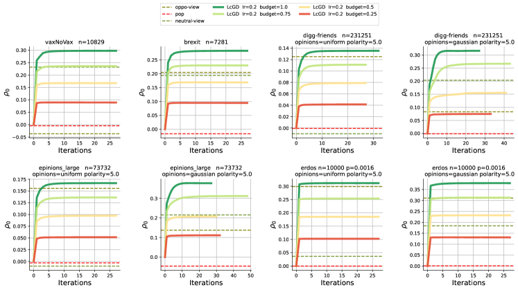
Figure 1. Reduction in polarization and disagreement (in the counterfactual scenario) vs number of iterations, using the stopping condition $\delta=10^{-6}|E|$. For vaxNoVax and Brexit networks, we have real-world estimated opinions. For the other semi-synthetic datasets we report both uniform and gaussian distributions of opinions.

Semidefinite programming. In SDP, we aim to minimize a linear function subject to constraints of the form $\mathbf{A}\mathbf{x}=\mathbf{b}$ and $\mathbf{X}\succeq 0$, where $\mathbf{X}$ is a symmetric matrix, and the notation $\mathbf{X}\succeq 0$ indicates that $\mathbf{X}$ is positive semidefinite. In the case of undirected graphs, the matrix variable $\mathbf{A}$ is positive semidefinite. To demonstrate that the problem can be formulated as an SDP, we refer to the classic textbook of Boyd and Vandenberghe (2004, Example 3.4, page 76). The general problem we want to solve can be written as

(16) $$\min_{t\in\mathrm{epi}\,f(\mathbf{A})}t,$$

where $t\in\mathbb{R}$, and the epigraph of the objective function $f(\mathbf{A})=\mathbf{s}^{\top}(2\mathbf{I}-\mathbf{A})^{-1}\mathbf{s}$ is defined as

$$\mathrm{epi}\,f =\{(\mathbf{s},2\mathbf{I}-\mathbf{A},t)\mid\mathbf{I}+\mathbf{L}\succ 0,\>\mathbf{s}^{\top}(2\mathbf{I}-\mathbf{A})^{-1}\mathbf{s}\leq t\}$$

$$=\{(\mathbf{s},2\mathbf{I}-\mathbf{A},t)\mid\begin{bmatrix}2\mathbf{I}-\mathbf{A}&\mathbf{s}\\ \mathbf{s}^{\top}&t\end{bmatrix}\succeq 0,\>2\mathbf{I}-\mathbf{A}\succ 0\},$$

where we utilize the Schur’s complement. The last condition represents a linear matrix inequality in $(\mathbf{s},2\mathbf{I}-\mathbf{A},t)$, and the set is convex. This convex-optimization problem can be efficiently solved, approximately within any constant factor, using various first-order methods such as SCS (O’donoghue et al., 2016) and ADMM (Wen et al., 2010).

To facilitate the solution process, several standard SDP libraries, including CVX (Grant and Boyd, 2014), implement these exact solvers. It is worth noting, however, that these libraries may encounter scalability issues, as highlighted in recent research (Majumdar et al., 2019).

5. Experimental evaluation

We structure our experimental evaluation to answer the following research questions:

• What is the reduction in polarization and disagreement for different input networks? How does this reduction compare to the equilibrium state with no interventions?

• What is the effect of network modularity and initial polarization on the behavior of the algorithm? What is the effect of the budget parameter?

• How does the algorithm perform for undirected graphs?

Table 1. Network statistics.

Network name	Type	# nodes	# edges	Description
brexit	R	7 281	530 608	retweets (UK Brexit referendum)
vaxNoVax	R	10 829	1 430 776	retweets (Italian vaccination debate)
Albert-Barabási	S	7 047	10 763	synthetic scale-free graph
SBM	S	9 999	81 867	synthetic stochastic block model
Erdős-Rényi	S	10 000	160 107	synthetic binomial graph
ego-twitter	SS	11 548	17 100	Twitter following network
facebook-wosn-wall	SS	37 082	260 307	Facebook posts to other user’s wall
soc-epinions1	SS	49 604	471 855	trust and distrust network
epinions	SS	73 732	767 982	trust network from Epinions
munmun	SS	464 882	834 548	Twitter mentions
digg-friends	SS	231 251	1 666 463	directed friendship graph of Digg
flickr-growth	SS	2 070 819	31 335 568	Flickr social network

5.1. Experimental setup

In this section, we describe our experimental pipeline. We begin by describing the types of data we consider. We then present our baselines and evaluation measures, and finally, we present the overall experimental scheme. Our code is made publicly available.

Table 2. Results on the reduction of polarization and disagreement for directed graphs with Gaussian opinion distribution, using a learning rate $\eta=0.2$ and stopping rule $\delta=10^{-6}|E|$.

Input configuration		$\rho_{\mathrm{eq}}$ ($\uparrow$ better)				$\rho_{0}$ ($\uparrow$ better)				Time (sec)
Network	Polarity	LcGD	neutral-view	oppo-view	pop	LcGD	neutral-view	oppo-view	pop	LcGD	neutral-view	oppo-view	pop
Albert-Barabási	1.0	0.2375	0.1688	0.0677	-0.0710	0.8195	0.8037	0.7784	0.7493	3.15	0.00	0.00	0.00
	5.0	0.4001	0.2215	0.2845	-0.1007	0.8008	0.7415	0.7624	0.6346	7.04	0.00	0.00	0.00
brexit	1.0	0.2824	0.1937	0.2045	-0.0162	0.8216	0.7996	0.8023	0.7474	43.08	0.02	0.04	0.02
	5.0	0.2824	0.1937	0.2045	-0.0162	0.8216	0.7996	0.8023	0.7474	38.09	0.02	0.06	0.03
digg-friends	1.0	0.1810	0.1164	0.0251	-0.0097	0.8287	0.8151	0.7960	0.7887	639.54	0.08	0.04	0.04
	5.0	0.3104	0.1931	0.0916	0.0039	0.7830	0.7461	0.7141	0.6865	354.45	0.07	0.07	0.06
ego-twitter	1.0	0.0747	0.0193	0.0159	-0.0114	0.8174	0.8065	0.8058	0.8004	60.03	0.00	0.00	0.00
	5.0	0.1478	0.0401	0.0540	-0.0137	0.6671	0.6250	0.6304	0.6040	79.31	0.00	0.00	0.00
epinions	1.0	0.2293	0.1657	0.0315	0.0152	0.8294	0.8154	0.7857	0.7821	740.10	0.03	0.02	0.02
	5.0	0.3816	0.2204	0.1446	-0.0494	0.8041	0.7530	0.7290	0.6676	281.98	0.02	0.02	0.02
Erdős-Rényi	1.0	0.2034	0.1435	0.0340	0.0009	0.8202	0.8063	0.7790	0.7710	7.71	0.00	0.00	0.00
	5.0	0.2623	0.1163	0.1919	0.0034	0.7527	0.7056	0.7294	0.6697	5.38	0.00	0.00	0.00
facebook-wosn-wall	1.0	0.2568	0.1719	0.0481	0.0009	0.8212	0.8007	0.7710	0.7596	334.43	0.01	0.01	0.01
	5.0	0.3898	0.2438	0.1697	0.0087	0.7213	0.6546	0.6208	0.5473	393.35	0.01	0.01	0.01
flickr-growth	1.0	0.1896	0.0999	0.0311	0.0162	0.8278	0.8087	0.7941	0.7910	3 373.66	2.27	0.70	0.96
	5.0	0.3385	0.2106	0.1413	0.0217	0.7578	0.7110	0.6856	0.6417	4 710.21	2.36	1.03	1.01
munmun	1.0	0.0982	0.0375	0.0152	-0.0008	0.8224	0.8105	0.8061	0.8029	383.99	0.04	0.02	0.02
	5.0	0.1944	0.0326	0.1058	0.0038	0.7048	0.6455	0.6724	0.6350	368.46	0.04	0.03	0.02
sbm	1.0	0.3174	0.2385	0.0421	-0.0018	0.8225	0.8020	0.7509	0.7395	56.68	0.00	0.00	0.00
	5.0	0.4641	0.3313	0.1851	-0.0070	0.7513	0.6898	0.6215	0.5326	107.88	0.00	0.00	0.00
soc-epinions1	1.0	0.2070	0.1402	0.0265	-0.0032	0.8285	0.8140	0.7894	0.7830	620.93	0.02	0.01	0.01
	5.0	0.3504	0.1929	0.1667	-0.0791	0.8033	0.7556	0.7477	0.6732	279.17	0.02	0.01	0.01
vaxNoVax	1.0	0.2976	0.2319	-0.0366	-0.0042	0.8318	0.8161	0.7519	0.7596	94.97	0.06	0.15	0.10
	5.0	0.2976	0.2319	-0.0366	-0.0042	0.8318	0.8161	0.7519	0.7596	100.95	0.06	0.12	0.12

Real-world data (R, in Table 2). We use two real-world networks from Twitter, along with corresponding opinions on social issues (Brexit and Vaccination) which were estimated with a supervised text-based classifier (Minici et al., 2022; Cossard et al., 2020). The opinion of a user is taken as the average opinion over all their tweets.

Synthetic data (S, in Table 2). We use three different types of network models: Erdős-Rényi, Albert-Barabási, and the stochastic block model. We also consider two types of opinion distributions: uniform in the interval $[-0.5,0.5]$ and Gaussian. To control the initial level of polarization, we incorporate one parameter that characterizes the bimodality of the distributions. First, for the uniform distribution, this parameter, denoted as $p$, is used to rescale each opinion value $z_{u}$ using the function $f(z_{u})=\mathrm{sign}(z_{u})|z_{u}|^{1/p}$. Second, to account for structural polarization within the network, we employ the Kernighan–Lin algorithm (Kernighan and Lin, 1970) to partition the network into two communities and assign to the nodes of each community opinions from two distinct Gaussian distributions. In this setting, the polarization parameter $p$ is proportional to the distance between the means of the two communities.

Semi-synthetic data (SS, in Table 2). We use public real-world networks that are semantically aligned with our study. To generate opinions, we follow the same approach as for synthetic data.

Methods. We refer to our method as LcGD, for Laplacian-constrained gradient descent. To enhance the efficiency of LcGD, we implement an acceleration technique using the ADAM optimizer (Kingma and Ba, 2014).

To evaluate LcGD against other methods, we implement three realistic baselines, which prioritize links involving specific types of nodes, namely, neutral nodes ($w_{u,v}\propto 1/|s_{u}|$), nodes with opposite views ($w_{u,v}\propto|s_{u}-s_{v}|$), and popular nodes ($w_{u,v}\propto d_{u}$).

Measures. We quantify the reduction in polarization and disagreement using two measures. First, we compare the objective function in Eq. (6) computed at equilibrium, with the objective function obtained at the equilibrium with the optimized weights. This measure, denoted as ${\rho_{\mathrm{eq}}}$, is defined as

(17) $${\rho_{\mathrm{eq}}}=1-\frac{P(\mathbf{z}^{*})+D(\mathbf{z}^{*},\mathbf{A}^{*})}{P(\mathbf{z})+D(\mathbf{z},\mathbf{A})}\,,$$

where $\mathbf{z}^{*}=(2\mathbf{I}-\mathbf{A}^{*})^{-1}\mathbf{s}$ is the equilibrium produced by the optimized adjacency matrix, and $\mathbf{z}=(2\mathbf{I}-\mathbf{A})^{-1}\mathbf{s}$ is the equilibrium produced by the original input matrix. This measure quantifies the reduction in polarization while accounting for the natural reduction in disagreement achieved by the FJ model. Additionally, we consider the reduction in polarization and disagreement with respect to the values produced by the innate opinions and the original input matrix. This measure, denoted as ${\rho_{0}}$, is defined as

(18) $${\rho_{0}}=1-\frac{P(\mathbf{z}^{*})+D(\mathbf{z}^{*},\mathbf{A}^{*})}{P(\mathbf{s})+D(\mathbf{s},\mathbf{A})}\,.$$

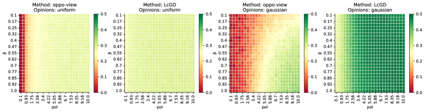
Figure 2. Modularity ($\beta:=$probability to connect two nodes in different communities) vs. polarization level in SBM network.

Evaluation scheme. Our evaluation scheme is as follows.

1. We sample equilibrium opinions $\mathbf{z}$ from a uniform/Gaussian distribution or, in the case of real datasets, we use the given opinions.

2. We normalize the adjacency matrix to make it row-stochastic.

3. We use the FJ model to estimate innate opinions as in Eq. (5).

4. We compute the optimal adjacency matrix $\mathbf{A}^{*}$ for each method and the reduction in polarization and disagreement using the two measures $\rho_{\mathrm{eq}}$ and $\rho_{0}$.

5.2. Results

RQ1: Performance. Our algorithm, LcGD, consistently outperforms the baselines in all input configurations. It achieves a significant reduction in polarization and disagreement ranging from 10% to 50% compared to the equilibrium with no intervention (measure $\rho_{\mathrm{eq}}$). Compared to the initial value (measure $\rho_{0}$), LcGD achieves an impressive reduction reaching up to 80%. As expected, the most consistent baseline is the one that promotes neutral connections, as it increases the visibility of non-polarized content. The baseline that strengthens connections between users with opposite views performs the best in polarized configurations with no echo chambers. On the other hand, promoting popular content can actually exacerbate polarization and disagreement, resulting in poor performance across all input instances.

As shown in Fig. 1 LcGD converges in a small number of iterations, typically fewer than 10, even for networks with over 2 million nodes, which corresponds to a runtime of approximately 10 minutes. Additionally, through a grid search for the learning rate, with values 0.2, 0.02, and 0.002, we find that a relatively large learning rate works well in terms of both time and performance.

RQ2: Effect of parameters. In practice, limited interventions in users’ feeds can be desirable. To address this, we conduct experiments (Fig.1) where we modify the input weights in the network by a fixed percentage. This approach results in an adjacency matrix that is a convex combination of the projected row-stochastic gradient and the input matrix at each iteration (line 11 in Alg. 1). Remarkably, LcGD outperforms the baselines in configurations with polarized and segregated communities, even when changing only 75% of the weights.

The LcGD algorithm demonstrates superior performance in highly-polarized configurations, both in terms of network structure (high modularity) and opinion distribution (high polarization). Such configurations mirror real-world social networks, making our approach an ideal solution for such instances. Conversely, less clustered structures, such as Erdős-Rényi graphs and uniform opinion distributions, do not exhibit a sufficiently-high level of polarization to support substantial reductions in the objective. Despite of this, as shown in Fig. 2, LcGD consistently surpasses alternative approaches even in situations with relatively low polarization levels. Additionally, the performance of LcGD remains unaffected by the modularity of the network, reflecting its robustness to real-world scenarios.

Table 3. Results on $\rho_{0}$ ($\uparrow$ better) for undirected graphs with two distributions of opinions (uniform and gaussian).

		gaussian		uniform
Network	nodes	LcGD	SCS	LcGD	SCS
Albert-Barabási graph	100	0.8154	0.7990	0.8568	0.8560
Erdős-Rényi graph	100	0.7677	0.7206	0.8584	0.8558
Aarhus CS department	61	0.7650	0.7481	0.8249	0.8272
dimacs10-football	115	0.7588	0.7293	0.8322	0.8358
political books	105	0.7046	0.6101	0.8439	0.8369
students cooperation	141	0.5324	0.5269	0.8462	0.8335

Table 4. Gradient descent scheme comparison on $\rho_{0}$ ($\uparrow$ better) for directed graphs with gaussian opinions.

	$\rho_{0}$		Time (sec)
Network	LcGD	simple GD	LcGD	simple GD
brexit	0.8216	0.8215	38.09	79.23
digg-friends	0.7830	0.7873	354.45	505.09
ego-twitter	0.6671	0.6655	79.31	94.21
epinions	0.8041	0.8071	281.98	969.03
vaxNoVax	0.8318	0.8299	100.95	193.51

RQ3: Undirected graphs. We also compare LcGD with the SDP approach (defined in Eq. (16)), using both synthetic and real-world undirected networks. We solve the SDP problem using the CVX library (Grant and Boyd, 2014) with the SCS solver (O’donoghue et al., 2016). Due to the computational limitations associated with the SDP approach (Majumdar et al., 2019), we limit the experiments to small networks. As discussed in Section 2, the SDP formulation can be viewed as a version of the method proposed by Musco et al. (Musco et al., 2018), adapted to accommodate a given graph topology. It is worth stressing that in this experiment, both the methods take in input an undirected graph, but while the SDP is forced to output a weighted undirected graph, our more general approach is allowed to assign different weights to $(i,j)$ and $(j,i)$.

As shown in Table 4, LcGD outperforms the SDP approach, especially in the case of Gaussian opinion distributions. For uniform opinion distributions, where there is a lack of structural polarization patterns, the two methods are on par, and in two configurations the SDP approach exhibits slightly better performance.

In summary, our method for directed graphs is also applicable to undirected graphs, where, by treating an undirected edge as the two corresponding directed links, it is possible to assign different importance weights to the content produced by user $i$ for the feed of user $j$ with respect to the content produced by $j$ for the feed of $i$. This flexibility, makes it to overperform the SDP method, which is optimal, but only for symmetric solutions.

Ablation study. We assess the impact of the ADAM optimizer through an ablation study where we use only the standard gradient-descent procedure. The results are presented in Table 4. We observe that both algorithms achieve comparable values of the objective, but LcGD, which uses the ADAM optimizer, converges faster than standard gradient descent.

6. Conclusions

Leveraging the Friedkin–Johnsen opinion-dynamics model, we presented a novel approach to minimize polarization and disagreement in a social network. This is done by re-weighting the relative importance of the accounts that a user follows, so as to calibrate the frequency with which the content produced by various accounts is shown to the user. By re-balancing the weight of existing links only, our approach preserves the total engagement of each user in the social network. We showed that our objective function is not matrix-convex, but the feasible set is convex, and we devised a scalable algorithm based on projected gradient descent. With an extensive experimental evaluation, we demonstrated the effectiveness of the proposed approach in its ability to minimize polarization and disagreement in large social networks.

While the paper contributes valuable insights, it is important to acknowledge some limitations. The absence of backfire-effect modeling (Wood and Porter, 2019) is inherent in the FJ model and restricts the approach’s ability to fully capture the complexities of polarization dynamics. Further research could explore incorporating this effect. Furthermore, it would be interesting to extend our approach to handle multiple topics and leverage additional features.

References

- (1)
- Abebe et al. (2021) Rediet Abebe, T-H HUBERT Chan, Jon Kleinberg, Zhibin Liang, David Parkes, Mauro Sozio, and Charalampos E Tsourakakis. 2021. Opinion dynamics optimization by varying susceptibility to persuasion via non-convex local search. ACM Transactions on Knowledge Discovery from Data (TKDD) 16, 2 (2021), 1–34.
- Acemoglu and Ozdaglar (2011) Daron Acemoglu and Asuman Ozdaglar. 2011. Opinion dynamics and learning in social networks. Dynamic Games and Applications 1 (2011), 3–49.
- Aslay et al. (2018) Çigdem Aslay, Antonis Matakos, Esther Galbrun, and Aristides Gionis. 2018. Maximizing the Diversity of Exposure in a Social Network. In IEEE International Conference on Data Mining, ICDM 2018, Singapore, November 17-20, 2018. 863–868.
- Bail et al. (2018) Christopher A Bail, Lisa P Argyle, Taylor W Brown, John P Bumpus, Haohan Chen, MB Fallin Hunzaker, Jaemin Lee, Marcus Mann, Friedolin Merhout, and Alexander Volfovsky. 2018. Exposure to opposing views on social media can increase political polarization. Proceedings of the National Academy of Sciences 115, 37 (2018), 9216–9221.
- Baumann et al. (2023) Fabian Baumann, Daniel Halpern, Ariel D Procaccia, Iyad Rahwan, Itai Shapira, and Manuel Wuthrich. 2023. Optimal Engagement-Diversity Tradeoffs in Social Media. arXiv preprint arXiv:2303.03549 (2023).
- Bessi et al. (2016) Alessandro Bessi, Fabiana Zollo, Michela Del Vicario, Michelangelo Puliga, Antonio Scala, Guido Caldarelli, Brian Uzzi, and Walter Quattrociocchi. 2016. Users polarization on Facebook and Youtube. PloS one 11, 8 (2016), e0159641.
- Bindel et al. (2015) David Bindel, Jon Kleinberg, and Sigal Oren. 2015. How bad is forming your own opinion? Games and Economic Behavior 92 (2015), 248–265.
- Boyd and Vandenberghe (2004) Stephen Boyd and Lieven Vandenberghe. 2004. Convex optimization. Cambridge university press.
- Brookes (2005) Mike Brookes. 2005. The matrix reference manual. Imperial College London 3 (2005), 16.
- Burden et al. (2015) Richard L Burden, J Douglas Faires, and Annette M Burden. 2015. Numerical analysis. Cengage learning.
- Chen et al. (2018) Xi Chen, Jefrey Lijffijt, and Tijl De Bie. 2018. Quantifying and minimizing risk of conflict in social networks. In Proceedings of the 24th ACM SIGKDD International Conference on Knowledge Discovery & Data Mining. 1197–1205.
- Cinus et al. (2022) Federico Cinus, Marco Minici, Corrado Monti, and Francesco Bonchi. 2022. The effect of people recommenders on echo chambers and polarization. In Proceedings of the International AAAI Conference on Web and Social Media, Vol. 16. 90–101.
- Cossard et al. (2020) Alessandro Cossard, Gianmarco De Francisci Morales, Kyriaki Kalimeri, Yelena Mejova, Daniela Paolotti, and Michele Starnini. 2020. Falling into the echo chamber: the Italian vaccination debate on Twitter. In Proceedings of the International AAAI conference on web and social media, Vol. 14. 130–140.
- Fletcher and Watson (1976) R Fletcher and GA Watson. 1976. Numerical analysis dundee 1975. Lecture notes in Mathematics 506 (1976), 73–89.
- Friedkin and Johnsen (1990) Noah E Friedkin and Eugene C Johnsen. 1990. Social influence and opinions. Journal of Mathematical Sociology 15, 3-4 (1990), 193–206.
- Garimella et al. (2017) Kiran Garimella, Aristides Gionis, Nikos Parotsidis, and Nikolaj Tatti. 2017. Balancing information exposure in social networks. Advances in neural information processing systems 30 (2017).
- Garimella et al. (2018) Kiran Garimella, Gianmarco De Francisci Morales, Aristides Gionis, and Michael Mathioudakis. 2018. Reducing Controversy by Connecting Opposing Views. In Proceedings of the Twenty-Seventh International Joint Conference on Artificial Intelligence, IJCAI 2018, July 13-19, 2018, Stockholm, Sweden. 5249–5253.
- Grant and Boyd (2014) Michael Grant and Stephen Boyd. 2014. CVX: Matlab software for disciplined convex programming, version 2.1.
- Hartman et al. (2022) Rachel Hartman, Will Blakey, Jake Womick, Chris Bail, Eli J Finkel, Hahrie Han, John Sarrouf, Juliana Schroeder, Paschal Sheeran, Jay J Van Bavel, et al. 2022. Interventions to reduce partisan animosity. Nature human behaviour 6, 9 (2022), 1194–1205.
- Haynsworth (1970) Emilie V Haynsworth. 1970. Applications of an inequality for the Schur complement. Proc. Amer. Math. Soc. 24, 3 (1970), 512–516.
- Interian et al. (2021) Ruben Interian, Jorge R Moreno, and Celso C Ribeiro. 2021. Polarization reduction by minimum-cardinality edge additions: Complexity and integer programming approaches. International Transactions in Operational Research 28, 3 (2021), 1242–1264.
- Kernighan and Lin (1970) Brian W Kernighan and Shen Lin. 1970. An efficient heuristic procedure for partitioning graphs. The Bell system technical journal 49, 2 (1970), 291–307.
- Kingma and Ba (2014) Diederik P Kingma and Jimmy Ba. 2014. Adam: A method for stochastic optimization. arXiv preprint arXiv:1412.6980 (2014).
- Kubin and von Sikorski (2021) Emily Kubin and Christian von Sikorski. 2021. The role of (social) media in political polarization: a systematic review. Annals of the International Communication Association 45, 3 (2021), 188–206.
- Majumdar et al. (2019) Anirudha Majumdar, Georgina Hall, and Amir Ali Ahmadi. 2019. A survey of recent scalability improvements for semidefinite programming with applications in machine learning, control, and robotics. arXiv preprint arXiv:1908.05209 (2019).
- Marumo et al. (2021) Naoki Marumo, Atsushi Miyauchi, Akiko Takeda, and Akira Tanaka. 2021. A Projected Gradient Method for Opinion Optimization with Limited Changes of Susceptibility to Persuasion. In Proceedings of the 30th ACM International Conference on Information & Knowledge Management. 1274–1283.
- Matakos et al. (2020) Antonis Matakos, Sijing Tu, and Aristides Gionis. 2020. Tell me something my friends do not know: Diversity maximization in social networks. Knowledge and Information Systems 62 (2020), 3697–3726.
- Minici et al. (2022) Marco Minici, Federico Cinus, Corrado Monti, Francesco Bonchi, and Giuseppe Manco. 2022. Cascade-based echo chamber detection. In Proceedings of the 31st ACM International Conference on Information & Knowledge Management. 1511–1520.
- Musco et al. (2018) Cameron Musco, Christopher Musco, and Charalampos E Tsourakakis. 2018. Minimizing polarization and disagreement in social networks. In Proceedings of the 2018 World Wide Web Conference. 369–378.
- Nikolov et al. (2015) Dimitar Nikolov, Diego FM Oliveira, Alessandro Flammini, and Filippo Menczer. 2015. Measuring online social bubbles. PeerJ computer science 1 (2015), e38.
- Nordström (2011) Kenneth Nordström. 2011. Convexity of the inverse and Moore–Penrose inverse. Linear algebra and its applications 434, 6 (2011), 1489–1512.
- O’donoghue et al. (2016) Brendan O’donoghue, Eric Chu, Neal Parikh, and Stephen Boyd. 2016. Conic optimization via operator splitting and homogeneous self-dual embedding. Journal of Optimization Theory and Applications 169 (2016), 1042–1068.
- Pariser (2011) Eli Pariser. 2011. The filter bubble: What the Internet is hiding from you. penguin UK.
- Petersen et al. (2008) Kaare Brandt Petersen, Michael Syskind Pedersen, et al. 2008. The matrix cookbook. Technical University of Denmark 7, 15 (2008), 510.
- Quattrociocchi et al. (2016) Walter Quattrociocchi, Antonio Scala, and Cass R Sunstein. 2016. Echo chambers on Facebook. Available at SSRN 2795110 (2016).
- Tu et al. (2020) Sijing Tu, Çigdem Aslay, and Aristides Gionis. 2020. Co-exposure Maximization in Online Social Networks. In Advances in Neural Information Processing Systems 33: Annual Conference on Neural Information Processing Systems 2020, NeurIPS 2020, December 6-12, 2020, virtual.
- Tucker et al. (2018) Joshua A Tucker, Andrew Guess, Pablo Barberá, Cristian Vaccari, Alexandra Siegel, Sergey Sanovich, Denis Stukal, and Brendan Nyhan. 2018. Social media, political polarization, and political disinformation: A review of the scientific literature. Political polarization, and political disinformation: a review of the scientific literature (March 19, 2018) (2018).
- Vicario et al. (2019) Michela Del Vicario, Walter Quattrociocchi, Antonio Scala, and Fabiana Zollo. 2019. Polarization and fake news: Early warning of potential misinformation targets. ACM Transactions on the Web (TWEB) 13, 2 (2019), 1–22.
- Wen et al. (2010) Zaiwen Wen, Donald Goldfarb, and Wotao Yin. 2010. Alternating direction augmented Lagrangian methods for semidefinite programming. Mathematical Programming Computation 2, 3-4 (2010), 203–230.
- Wood and Porter (2019) Thomas Wood and Ethan Porter. 2019. The elusive backfire effect: Mass attitudes’ steadfast factual adherence. Political Behavior 41 (2019), 135–163.
- Xia et al. (2011) Haoxiang Xia, Huili Wang, and Zhaoguo Xuan. 2011. Opinion dynamics: A multidisciplinary review and perspective on future research. International Journal of Knowledge and Systems Science (IJKSS) 2, 4 (2011), 72–91.
- Xu et al. (2022) Wanyue Xu, Liwang Zhu, Jiale Guan, Zuobai Zhang, and Zhongzhi Zhang. 2022. Effects of Stubbornness on Opinion Dynamics. In Proceedings of the 31st ACM International Conference on Information & Knowledge Management. 2321–2330.
- Zha et al. (2020) Quanbo Zha, Gang Kou, Hengjie Zhang, Haiming Liang, Xia Chen, Cong-Cong Li, and Yucheng Dong. 2020. Opinion dynamics in finance and business: a literature review and research opportunities. Financial Innovation 6 (2020), 1–22.
- Zhu et al. (2021) Liwang Zhu, Qi Bao, and Zhongzhi Zhang. 2021. Minimizing Polarization and Disagreement in Social Networks via Link Recommendation. Advances in Neural Information Processing Systems 34 (2021), 2072–2084.