Probing chiral and flavored $Z^{\prime}$ from cosmic bursts through neutrino interactions

Abstract

The origin of tiny neutrino mass is an unsolved puzzle leading to a variety of phenomenological aspects beyond the Standard Model (BSM). Among several interesting attempts, $U(1)$ gauge extension of Standard Model (SM) is a simple and interesting set-up where the so-called seesaw mechanism is incarnated by the addition of three generations of right-handed neutrinos followed by the breaking of $U(1)$ and electroweak symmetries. Such scenarios are anomaly free in nature appearing with a neutral BSM gauge boson ($Z^{\prime}$). In addition to that, there comes another open question regarding the existence of a non-luminous, hitherto unidentified object called Dark Matter (DM) originating from the measurement of its relic density. To explore properties of $Z^{\prime}$, we focus on chiral and flavored scenarios where $Z^{\prime}-$neutrinos interaction could be probed in the context of cosmic explosions like gamma-ray burst (GRB221009A, so far the highest energy), blazar (TXS 0506+056) and Active galaxy (NGC1068) respectively. The neutrino antineutrino annihilation produces electron-positron pair which could energize GRB through energy deposition. Taking the highest energy GRB under consideration and estimating the energy deposition rates we constrain $Z^{\prime}$ mass $(M_{Z^{\prime}})$ and the additional $U(1)$ coupling $(g_{X})$ for chiral and flavored scenarios in the Schwarzchild, Hartle-Thorne and modified gravity frameworks. On the other hand, adding viable and alternative DM candidates in these models we study neutrino-DM scattering mediated by $Z^{\prime}$ in the $t-$ channel and estimate constraints on $g_{X}-M_{Z^{\prime}}$ plane using observed data of high energy neutrinos from cosmic blazar and active galaxy at the IceCube experiment. We compare our results with bounds obtained from different scattering, beam-dump and $g-2$ experiments.

I Introduction

Experimental observations of tiny neutrino mass and flavor mixing [1] allow the Standard Model (SM) of particle physics to step beyond. Additionally, from the studies of bullet cluster, large-scale cosmological data and galaxy rotation curve we come to know that roughly one-fourth of the energy budget of the Universe has been apportioned to some non-luminous objects called dark matter (DM), which strongly suggest going beyond the SM (BSM) [2, 3, 4, 5]. A simple but interesting way to explain the origin of tiny neutrino mass is the seesaw mechanism [6, 7, 8, 9, 10] where SM is extended by adding singlet heavy Right Handed Neutrinos (RHN). The latter is an appropriate realization of the idea of a dimension five operator within the SM framework [11], where a heavy mass scale can be integrated out, followed by the violation of the lepton number by two units.

Apart from the particle extension of the SM, a simple $U(1)$ gauge extension of the SM, SM$\otimes U(1)$, can also be a suitable choice to explain the origin of tiny neutrino mass at the tree level and flavor mixing. Such scenarios can accommodate potential DM candidates. Interestingly such scenarios give rise to a massive neutral BSM gauge boson, commonly known as $Z^{\prime}$, after the breaking of the $U(1)$ symmetry. For example, we consider a pioneering scenario called B$-$L (baryon minus lepton) [12, 13, 14, 15], where three generations of SM-singlet RHNs are introduced to achieve a theory free from the gauge and mixed gauge-gravity anomalies, resulting in the $Z^{\prime}$ interactions with the left and right-handed fermions of the model in the same way by leading to a vector-like scenario. In this model set-up, there is an SM-singlet scalar field that acquires vacuum expectation value (VEV) through the breaking of B$-$L symmetry. Hence the Majorana mass term for the RHNs is generated helping the light neutrinos to achieve tiny masses through the seesaw mechanism followed by flavor mixing.

Another interesting aspect in this matter could be a general $U(1)_{X}$ extension of the SM where we introduce three RHNs to cancel the gauge and mixed gauge-gravity anomalies which leads to a basic and interesting behavior where left and right-handed fermions interact differently with the neutral gauge boson $Z^{\prime}$ involved in this model, manifesting the chiral nature of this model from a variety of aspects including heavy neutrino production at the high energy colliders [16], neutrino-electron and neutrino-nucleon scattering [17, 18] and different beam dump experiments including proposed FASER, ILC-beam dump and DUNE [19]. In this scenario, a SM-singlet scalar field is considered, which obtains a (VEV) following the general breaking of the $U(1)$ symmetry. This symmetry breaking leads to the generation of Majorana masses for the heavy neutrinos, giving rise to the see-saw mechanism responsible for generating small neutrino masses and flavor mixing. In addition to that, we consider two more varieties of general $U(1)$ extension of the SM commonly known as $U(1)_{xq-\tau_{R}^{3}}$ and $U(1)_{q+xu}$ scenarios [20]. In the first case, we fixed general $U(1)$ charges for the RHNs as well as the SM-singlet BSM scalar field and [21, 22] whereas in the second one we fix general $U(1)$ charge for the left-handed fermion doublets of the SM, respectively. Apart from the general $U(1)$ extensions we also consider some well-known flavored scenarios. In this case, we first consider $L_{i}-L_{j}$ scenarios where particular two flavors are charged under the additional $U(1)$ gauge group, however, the third generation is not. If the $i$th generation is positively charged, then the $j$th generation will be negatively charged under the $U(1)$ extension [23, 24, 25, 26, 27]. The remaining fields are uncharged under this new gauge group. There is another alternative flavored scenario, namely B$-3L_{i}$ [28, 29, 30]. Here quark charges are their respective baryon numbers where the $i$th generation leptonic charge is 3 and the remaining leptonic generations are uncharged under the flavored $U(1)$ gauge groups. The fermions charged under the flavored gauge group only interact with $Z^{\prime}$ boson. These scenarios also contain SM-singlet scalar which acquires VEV and gives rise to the Majorana mass term for the RHNs which further generates the tiny neutrino mass through the seesaw mechanism.

In these models, $Z^{\prime}$ interacts with the charged leptons and neutrinos. Depending on the choice of model structure, $Z^{\prime}$ can interact with quarks and these interactions could be flavor dependent. It has interesting motivation in the neutrino-antineutrino annihilation process where the contribution from $Z^{\prime}$ plays an important role in electron-positron pair production along with the SM gauge boson mediated processes. It has been pointed out in [31] that electron neutrinos evolve from the accreting primary member and the anti-neutrinos appear from the disrupted secondary member of a Neutron Star (NS) binary system accelerating its collapse and emitting huge energy in the form of Gamma-Ray Burst (GRB). These neutrinos and antineutrinos could annihilate into electrons and positrons out of the orbital plane. Hence neutrino antineutrino annihilation causing electron-positron pair production is thought to energize GRB of the $\mathcal{O}(\geq 10^{51}\rm{erg})$ above the neutrino-sphere of a type-II supernova and it has been studied over decades in [32, 33, 34, 35, 36, 37, 38] by analyzing energy deposition rate. The strong gravitational field effects were investigated in [39, 40] and results showed that the efficiency of the neutrino-antineutrino annihilation process, compared to the Newtonian calculations, may enhance up to a factor of $30$ in case of collapsing NS. The energy deposition rate for an isothermal accretion disk in a Schwarzchild or Kerr metric was considered in [41, 42]. Time-dependent models in which black hole accretion disks evolving as a remnant of NS-mergers have been studied in [43, 44, 45, 46, 47] while other models include pair-annihilation during the evolution [48, 49, 50, 51]. These works suggest that neutrino-antineutrino annihilation in general relativity models may not be efficient enough to power GRBs. In this respect, the Blandford-Znajek process [52] could be a promising mechanism for launching jets from spinning supermassive black hole (BH) powering accreting supermassive BH. However, recently, a different perspective has been proposed for energizing GRBs. The neutrino-antineutrino annihilation into electron-positron pair emitted from the surface of a neutron star or accretion disk is studied in modified theories of gravity [53, 54]. Here a mechanism of neutrino heating involves neutrino-antineutrino annihilation, neutrino-lepton scattering and neutrino capture [55, 56, 57, 58]. In such a case, the energy deposition rate can increase by several orders of magnitude, opening a possibility to probe or to constrain extended theories of gravity in GRBs. In this context, we mention that recently an energetic GRB, named as ‘GRB 221009A’, has been observed [59, 60, 61, 62, 63, 64, 65] having isotropic energy of $E_{iso}\simeq 1.2\times 10^{55}$ erg [59] which can be applied in order to constrain the effect of neutrino energy deposition involving $Z^{\prime}$ mediated process in the framework of general relativity involving Newtonian, Schwarzchild and Hartle-Thorne metrics and modified gravity models like Born-Infield Reissner-Nordstorm [66] and charged Galileon [67].

A remarkable concurrence of neutrino emission with gamma rays was observed from the blazar TXS 0506+056 by the IceCube [68], where a neutrino was observed with an energy around 290 TeV (IC 0922A event), with jets pointing towards the Earth. High energy neutrinos from distant astrophysical sources pass through a dense spike of DM [69, 70] neighbouring the central black hole. As a result, there is a high chance of neutrino-DM scattering in this scenario which is a comparatively challenging scenario because observing neutrino is tough. Therefore we consider high-energy neutrinos from astrophysical sources. These high-energy neutrinos could boost DM particles if they are light, so that they can be detected in the ground-based experiments [71, 72, 73, 74, 75, 76, 77] involving a variety of DM scattering processes. The general $U(1)$ extensions of the SM can contain potential DM candidates under proper gauge structure. Such DM candidates can be charged under the $U(1)_{X}$ gauge group and as a result they potentially interact with $Z^{\prime}$. In these models, the lepton doublets are charged under $Z^{\prime}$, therefore neutrino-DM interactions in the $t-$channel process can be constrained using observed data from IceCube. Neutrino-DM scattering is under scanner for a long period of time through setting limits on the interactions considering the high energy neutrinos pass through DM staring from blazar before reaching to the earth [78, 79, 80, 81]. In this article, we perform model-dependent analyses of neutrino-DM scattering in the context of general $U(1)$ extension of the SM where neutrino-$Z^{\prime}$ and DM-$Z^{\prime}$ interactions depend on the general $U(1)$ charges manifesting the chiral nature of the model. Hence the $Z^{\prime}$ interactions could be constrained using neutrino flux from confirmed and reported IceCube data [68].

IceCube collaboration recently observed a point-like steady-state source of high energy neutrinos from a nearby active galaxy called NGC 1068 [82], a radio galaxy in nature and jets pointing about $90^{\degree}$ away from line of sight [83, 84], posting a landmark direct evidence of tera-electron volt neutrino emission. As a result, the Earth is exposed to equatorial emissions perpendicular to the jet. In this analysis, IceCube observed $79^{+22}_{-20}$ neutrinos from NGC 1068 at a significance of 4.2$\sigma$ having energies between 1 TeV to 15 TeV. At the galactic center there is a supermassive black hole which could be surrounded by a dense DM spike obstructing the emitted neutrinos, and resulting in neutrino-DM interaction which further empowers the emission of neutrinos. This mechanism depends on the region closer or away from the supermassive black hole allowing DM spike to play a very crucial role. Neutrinos and DM candidates are weakly coupled particles which might lead to weakened interactions in cosmology, astrophysics [85, 86, 87, 88, 89, 90, 91, 92, 93, 94, 95, 96] and direct detection of boosted DM candidate [97, 98, 99, 100, 101, 102] irrespective of ways considering a model dependant framework and model-independent framework respectively. In this context, neutrino-DM interaction can be probed utilizing the observed high-energy neutrinos emitted from Active Galactic Nuclei (AGN). An interesting approach of constraining neutrino-DM interaction has been studied in [103] using a vector interaction under B$-$L framework. In this paper, to explore neutrino-DM interaction, we employ a general $U(1)$ extension of the SM where $Z^{\prime}$ can interact with neutrinos and potential DM candidates. We consider three types of potential DM candidates, for example, complex scalar [104, 105, 106, 107], Majorana [108, 109, 110] and Dirac fermions [111, 112]. After anomaly cancellation, we find that general $U(1)_{X}$ affects these vertices glaring chiral property of the interactions exchanging $Z^{\prime}$ in the $t-$channel.

In our paper, we estimate bounds on the general $U(1)$ coupling $g_{X}$ with respect to $Z^{\prime}$ studying GRBs, and comparing the enhancement due to the involvement of $Z^{\prime}$ under general relativity and modified gravity models. To study neutrino-DM scattering using blazar and AGN data from IceCube, we solve, following Refs. [113, 114, 115, 72, 116], the cascade equation in order to obtain bounds on $g_{X}$ and $Z^{\prime}$ mass plane. These bounds will manifest the chiral nature of $Z^{\prime}$ due to different $U(1)$ charge assignments of the fermions depending on the model structure. Finally, we compare our results with existing bounds from neutrino-electron scattering from TEXONO [117], BOREXINO [118, 119], muon neutrino and muon anti-neutrino-electron scattering from CHARM-II [120, 121], coherent elastic neutrino-nucleus scattering from COHERENT experiment [122, 123, 124], neutrino magnetic moment experiment from GEMMA [125, 126], proton beam dump experiments like CHARM [127], Nomad [128], $\nu-$cal [129, 130] and electron/ positron beam dump experiments like Orsay [131], KEK [132], E141 [133], E137 [134], NA64 [135], E774 [136] and neutrino decay experiment like PS191 [137, 138, 139], respectively. In addition to these experiments, we consider long-lived particle search [140, 141, 142, 143] and dark photon search [144, 145] from LHCb, visible [146] and invisible [147] decay of dark photon in BaBar experiment and prompt production of GeV scale dark resonance search in CMS [148] to estimate bounds on the general $U(1)$ coupling with respect to $Z^{\prime}$ mass for different general $U(1)$ charges providing complementarity. In this region, bounds can be estimated from KLOE experiment to study light vector boson decay [149, 150, 151] into muon pair and a pair of charged pion, light gauge boson search from MAMI detector by A1 collaboration [152, 153] using its decay into electron-positron pair and finally studying the decay of dark photons into electron-positron and muon anti-muon pairs in association with a photon from Initial State Radiation (ISR), respectively. In this context, we also mention that experimental constraints from NA48/2 [154] are obtained studying dark photon decay into neutral pions, dark photon search from electron-nucleus fixed target experiment from APEX experiment [155], where the electron-positron pair is produced from a radiated dark gauge boson, dark photon search at the HEADS experiment [156] from its decay into electron-positron pair, dark photon search from neutral meson decay from PHENIX experiment [157], dark photon search from the WASA-at-COSY experiment from electron-positron final state [158]. BESII also performed searches of dark photons within a range of 1.4 GeV to 3.5 GeV which can be useful to estimate constraints on general $U(1)$ coupling with respect to $Z^{\prime}$ mass [159]. We recast bounds on general $U(1)$ coupling from LEP searches of di-muon [160, 161, 162], dijet [163] and dilepton searches from heavy resonance from CMS [164] and ATALS [165, 166] which constrain the parameter space for heavy neural gauge boson.

We arrange our paper in the following way. We describe the BSM scenarios involving the flavored and chiral models in Sec. II. The aspects of neutrino heating have been described in Sec. III followed by the analysis involving general relativity and modified gravity. Neutrino-DM scattering has been discussed using blazar and AGN data from IceCube in Sec. IV. We discuss the results in Sec. V and finally conclude the paper in Sec. VI.

II Beyond the standard model scenarios

A general $U(1)$ extension of the SM involves three generations of RHNs which are singlet under the SM gauge group. These RHNs help in solving gauge and mixed gauge-gravity anomalies followed by the generation of neutrino mass through the seesaw mechanism as considered in this paper. After anomaly cancellation, we find that general $U(1)$ charges are different for the left and right-handed fermions. These charges are generation independent. In addition to this setup, we consider flavored scenarios where all three generations of leptons do not have equal charges under the $U(1)$ gauge group, however, like the general $U(1)$ scenarios, they also have three RHNs which participate in neutrino mass generation mechanism through the seesaw mechanism.

II.1 General U$(1)$ extensions

The extension of the SM using a general $U(1)_{X}$ gauge group can involve three generations of the SM singlet RHNs and a BSM scalar which is singlet under the SM gauge group. To cancel the gauge and mixed gauge gravity anomalies [167, 168], we introduce three generations of the RHNs. The $U(1)$ symmetry is broken by the VEV of the SM singlet BSM scalar. After the $U(1)$ symmetry is broken, the Majorana mass term of the RHNs will be generated. These RHNs help to generate the mass of the light neutrinos satisfying the neutrino oscillation data and flavor mixing. The particle contents of general $U(1)$ extensions of the SM are given in Tab. 1.

Fields	$SU(3)_{c}\otimes SU(2)_{L}\otimes U(1)_{Y}$	$U(1)_{X}$	$U(1)_{xq-\tau_{R}^{3}}$	$U(1)_{q+xu}$
$q_{L}^{i}$	$(3,2,\frac{1}{6})$	$x_{q}=\frac{1}{6}x_{H}+\frac{1}{3}x_{\Phi}$	$x$	$\frac{1}{3}$
$u_{R}^{i}$	$(3,1,\frac{2}{3})$	$x_{u}=\frac{2}{3}x_{H}+\frac{1}{3}x_{\Phi}$	$-1+4x$	$\frac{x}{3}$
$d_{R}^{i}$	$(3,1,-\frac{1}{3})$	$x_{d}=-\frac{1}{3}x_{H}+\frac{1}{3}x_{\Phi}$	$1-2x$	$\frac{2-x}{3}$
$\ell_{L}^{i}$	$(1,2,-\frac{1}{2})$	$x_{\ell}=-\frac{1}{2}x_{H}-x_{\Phi}$	$-3x$	$-1$
$e_{R}^{i}$	$(1,1,-1)$	$x_{e}=-x_{H}-x_{\Phi}$	$1-6x$	$-(\frac{2+x}{3})$
$H$	$(1,2,-\frac{1}{2})$	$-\frac{1}{2}x_{H}$	$1-3x$	$\frac{1-x}{3}$
$N^{j}$	$(1,1,0)$	$x_{N}=-x_{\Phi}$	$-1$	$\frac{-4+x}{3}$
$\Phi$	$(1,1,0)$	$2\;x_{\Phi}$	$2$	$-2(\frac{-4+x}{3})$

Table 1: Particle content and charge assignments for minimal $U(1)$ extensions of the SM. Two new SM singlet fields $N$ (fermion) and $\Phi$ (scalar) are added to the SM particle content where ${i,j}$ are the flavour indices for three generations. $x_{H}$, $x_{\Phi}$ and $x$ are free parameters of the models.

The general charges are related to each other from the following gauge and mixed gauge-gravity anomaly cancellation conditions:

$$\left[{\rm SU}(3)_{C}\right]^{2}\otimes{\rm U}(1)_{X} \ : 2x_{q}-x_{u}-x_{d} \ =\ 0~{},$$

$$\left[{\rm SU}(2)_{L}\right]^{2}\otimes{\rm U}(1)_{X} \ : 3x_{q}+x_{\ell} \ =\ 0~{},$$

$$\left[{\rm U}(1)_{Y}\right]^{2}\otimes{\rm U}(1)_{X} \ : x_{q}-8x_{u}-2x_{d}+3x_{\ell}-6x_{e} \ =\ 0~{},$$

$$\left[{\rm U}(1)_{X}\right]^{2}\otimes{\rm U}(1)_{Y} \ : {x_{q}}^{2}-{2x_{u}}^{2}+{x_{d}}^{2}-{x_{\ell}}^{2}+{x_{e}}^{2} \ =\ 0~{},$$

$$\left[{\rm U}(1)_{X}\right]^{3} \ : {6x_{q}}^{3}-{3x_{u}}^{3}-{3x_{d}}^{3}+{2x_{\ell}}^{3}-{x_{N}}^{3}-{x_{e}}^{3} \ =\ 0~{},$$

$$\left[{\rm grav.}\right]^{2}\otimes{\rm U}(1)_{X} \ : 6x_{q}-3x_{u}-3x_{d}+2x_{\ell}-x_{N}-x_{e} \ =\ 0~{},$$ (1)

respectively. We write the Yukawa interactions following the SM$\otimes$ $U(1)_{X}$ gauge interactions in the following way as

$${\cal L}^{\rm Yukawa}=-Y_{u}^{\alpha\beta}\overline{q_{L}^{\alpha}}Hu_{R}^{\beta}-Y_{d}^{\alpha\beta}\overline{q_{L}^{\alpha}}\tilde{H}d_{R}^{\beta}-Y_{e}^{\alpha\beta}\overline{\ell_{L}^{\alpha}}\tilde{H}e_{R}^{\beta}-Y_{\nu}^{\alpha\beta}\overline{\ell_{L}^{\alpha}}HN_{R}^{\beta}-Y_{N}^{\alpha}\Phi\overline{(N_{R}^{\alpha})^{c}}N_{R}^{\alpha}+{\rm h.c.}~{}$$ (2)

where $H$ is the SM Higgs doublet, and $\tilde{H}=i\tau^{2}H^{*}$ with $\tau^{2}$ being the second Pauli matrix. We estimate the following conditions using $U(1)_{X}$ neutrality using the Yukawa interactions from Eq. 2 as

$$\frac{1}{2}x_{H}=-x_{q}+x_{u}\ =\ x_{q}-x_{d}\ =\ x_{\ell}-x_{e}=\ -x_{\ell}+x_{\nu}~{};~{}~{}~{}~{}-2x_{\Phi} = 2x_{N}~{}.$$ (3)

Finally, solving Eqs. 1 and 3, we express the $U(1)_{X}$ charges of the particles in terms of $x_{H}$ and $x_{\Phi}$. Hence, we find $U(1)_{X}$ charges of the SM charged fermions can be expressed as a linear combination of the $U(1)_{Y}$ and B$-$L charges implying left and right-handed fermions differently charged under the general $U(1)_{X}$ gauge group manifesting a chiral nature. We find that fixing $x_{\Phi}=1$ with $x_{H}=-2$, the $U(1)_{X}$ charges of the left-handed fermions reduce to zero converting the model into a $U(1)_{\rm R}$ scenario, and with the same $x_{\Phi}$ but vanishing $x_{H}$, the $U(1)_{X}$ charge assignment reduces into that of the B$-$L model. We find for fixed $x_{\Phi}=1$ with $x_{H}=-1$ the $U(1)_{X}$ charge of $e_{R}^{i}$ will be zero, for $x_{H}=-0.5$ and $1$, the $U(1)_{X}$ charge of $u_{R}^{i}$ and $d_{R}^{i}$ will be zero, respectively.

There is an alternative set-up of the general $U(1)_{X}$ scenario in which we fix the charge of the left-handed quark doublet $x_{q}$ as $x$, the charge of the RHN $x_{\nu}$ as $-1$ and the $U(1)$ charge of the BSM scalar $\Phi$ as $2$. Considering these choices and using Eq. 1, and following the Yukawa interactions given in Eq. 2, we solve the charges of the other SM particles. It actually rescales the $U(1)$ charges and we call it $U(1)_{xq-\tau^{3}_{R}}$ whose charges correspond to $6xY-\tau_{R}^{3}$. Taking $x=0$ and $x=\frac{1}{3}$, we find the $U(1)_{R}$ and $U(1)_{\rm B-L}$ scenarios, respectively. If we use $x=\frac{1}{4}$ and $\frac{1}{2}$, we find that the $U(1)_{xq-\tau^{3}_{R}}$ charges of $u_{R}^{i}$ and $d_{R}^{i}$ will be zero. If we use $x=\frac{1}{6}$ the U(1)${}_{xq-\tau^{3}_{R}}$ charge of $e_{R}^{i}$ will be zero. The charges of the $U(1)_{xq-\tau^{3}_{R}}$ gauge group is a minimal scenario as it has been stated in Tab. 1. Solving the anomaly cancellation conditions, we can have different charge assignments for $u_{R}$ and $d_{R}$, too. The corresponding alternative charge assignments will be $x_{u}=1-2x$ and $x_{d}=4x-1$ respectively, however, this solution is not mentioned in our paper because this demands an extension of the scalar sector of using doublets bypassing the minimal nature of models [20].

In Tab. 1 we write another scenario $U(1)_{q+xu}$ from [21, 22], where we fix the U$(1)$ charge of the left-handed quark doublet $x_{q}$ as $\frac{1}{3}$ assignments left-handed lepton doublet charge $x_{\ell}$ as $-1$ and we find these charges are considered to be identical with the B$-$L scenario. Now using the anomaly cancellation conditions stated in Eq. 1 and following the Yukawa interactions from Eq. 2, we derive the U(1)_q+xu charge assignments for the rest of the fermion and scalar sectors of the model. In this case, considering $x=1$, we could reduce the B$-$L charge assignments of the particles. However, we can not obtain the $U(1)_{\rm R}$ scenario playing with $x$. If we put $x=0$, then the charge of $u_{R}^{i}$ under $U(1)_{q+xu}$ gauge group will be zero. For $x=2$ we find the same for $d_{R}^{i}$. Similarly, if we impose a choice of $x=-2$ the $U(1)_{q+xu}$ charge of $e_{R}^{i}$ will be zero. In addition we comment that for $x=-1$, the $U(1)_{\chi}$ scenario follows from $SO(10)$ grand unification.

The renormalizable scalar potential in a singlet scalar extended scenario under a general $U(1)$ extension of SM can be written as

$$V\ =\ m_{h}^{2}(H^{\dagger}H)+\lambda_{H}(H^{\dagger}H)^{2}+m_{\Phi}^{2}(\Phi^{\dagger}\Phi)+\lambda_{\Phi}(\Phi^{\dagger}\Phi)^{2}+\lambda^{\prime}(H^{\dagger}H)(\Phi^{\dagger}\Phi)~{},$$ (4)

where $H$ is the SM Higgs doublet and $\Phi$ is the SM-singlet scalar fields where. Moreover, we can approximate $\lambda^{\prime}$ to be very small according to [169]. After breaking of the $U(1)_{X}$ gauge and electroweak symmetries, the scalar fields $H$ and $\Phi$ develop their vacuum expectation values (VEVs) as

$$\braket{H}\ =\ \frac{1}{\sqrt{2}}\begin{pmatrix}v+h\\ 0\end{pmatrix}~{},\quad{\rm and}\quad\braket{\Phi}\ =\ \frac{v_{\Phi}+\phi}{\sqrt{2}}~{}$$ (5)

where at the potential minimum the electroweak scale is demarcated as $v=246$ GeV and $v_{\Phi}$ is taken to be a free parameter. The breaking of the general $U(1)$ generates the mass of the $Z^{\prime}$ which is given by

$$M_{Z^{\prime}}=g_{X}\sqrt{4x_{\Phi}^{2}v_{\Phi}^{2}+x_{H}^{2}v^{2}}~{}.$$ (6)

The mass $M_{Z^{\prime}}$ in (6) reduces to $M_{Z^{\prime}}\simeq 2g_{X}x_{\Phi}v_{\Phi}$ for $v_{\Phi}\gg v$. Here we consider $x_{\Phi}=1$ without the loss of generality. The quantity $M_{Z^{\prime}}$ is a free parameter and $g_{X}$ is the general $U(1)$ coupling considered for the cases shown in Tab. 1. From the Yukawa interactions given in Eq. 2, we find that the RHNs interact with the SM-singlet scalar field $\Phi$. This Yukawa interaction generates Majorana mass term for heavy neutrinos after the general $U(1)$ symmetry is broken. After the electroweak symmetry breaking, the Dirac mass term is generated from the interaction term among the SM like Higgs doublet, SM lepton doublet and the SM-singlet RHN. These two mass terms finally switch on the seesaw mechanism to originate the tiny neutrino masses and flavor mixing. Using the symmetry breaking and Eq. 2 we write down the Majorana and Dirac mass terms in the following as

$$m_{N_{R}^{\alpha}}\ =\ \frac{Y^{\alpha}_{N}}{\sqrt{2}}v_{\Phi},\,\,\,\,\,\,\,\,m_{D}^{\alpha\beta}\ =\ \frac{Y_{\nu}^{\alpha\beta}}{\sqrt{2}}v~{}$$ (7)

respectively. Hence we obtain the neutrino mass mixing as

$$m_{\nu}=\begin{pmatrix}0&m_{D}\\ m_{D}^{T}&m_{N}\end{pmatrix}~{}$$ (8)

and diagonalizing Eq. 8 we obtain the light neutrino mass eigenvalues as $-m_{D}m_{N}^{-1}m_{D}^{T}$. The neutrino mass generation mechanism is not the point of interest of this papers. Therefore, we are not investigating the properties of the light and heavy neutrinos in this article.

We concentrate on the $Z^{\prime}$ interaction with the SM leptons under general $U(1)$ scenarios. From the above scenarios shown in Tab. 1, we find that the left and right handed SM fermions interact with $Z^{\prime}$ differently due to the presence of general $U(1)$ charges. Hence the interaction Lagrangian between the $Z^{\prime}$ boson and the SM fermions $(f)$ can be written as

$$\mathcal{L}^{f}=-g_{X}(\overline{f_{L}}\gamma^{\mu}q_{f_{L}}f_{L}+\overline{f_{R}}\gamma^{\mu}q_{f_{R}}f_{R})Z_{\mu}^{\prime}~{}$$ (9)

where $f$ includes SM quarks and leptons. The quantities $q_{f_{L}}$ and $q_{f_{R}}$ are the general $U(1)$ charges of the SM left and right handed fermions written in Tab. 1. Hence, the interactions between $Z^{\prime}$ and the SM fermions depend on the general U$(1)$ charges expressing the chiral nature of the model. Finally, we calculate the partial decay widths of $Z^{\prime}$ into different SM fermionic modes for a single generation as

$$\Gamma(Z^{\prime}\to\bar{f}f) =N_{C}\frac{M_{Z^{\prime}}g_{X}^{2}}{24\pi}\left[\left(q_{f_{L}}^{2}+q_{f_{R}}^{2}\right)\left(1-\frac{m_{f}^{2}}{M_{Z^{\prime}}^{2}}\right)+6q_{f_{L}}q_{f_{R}}\frac{m_{f}^{2}}{M_{Z^{\prime}}^{2}}\right]~{},$$ (10)

where $m_{f}$ is the SM fermion mass and $N_{C}=1$ for the SM leptons and $3$ for the SM quarks representing the color factor. The partial decay width of the $Z^{\prime}$ into a pair of light neutrinos of single generation is given by

$$\Gamma(Z^{\prime}\to\nu\nu)=\frac{M_{Z^{\prime}}g_{X}^{2}}{24\pi}q_{f_{L}}^{2}~{}$$ (11)

where we neglect the effect of tiny neutrino mass and $q_{f_{L}}$ stands for the $U(1)_{X}$ charge of the SM lepton doublet. In general $U(1)$ extended SM scenarios, the $Z^{\prime}$ gauge boson decays into a pair of heavy Majorana neutrinos following the interaction term

$$\mathcal{L}_{N}=-g_{X}q_{N_{R}}\overline{N}\gamma_{\mu}\gamma_{5}P_{R}NZ_{\mu}^{\prime}.$$ (12)

Hence we calculate the corresponding partial decay width for a single generation of the heavy neutrino pair as

$$\Gamma(Z^{\prime}\to N_{R}^{\alpha}N_{R}^{\alpha})=\frac{M_{Z^{\prime}}g_{X}^{2}}{24\pi}q_{N_{R}}^{2}\left(1-\frac{4M_{N}^{2}}{M_{Z^{\prime}}^{2}}\right)^{\frac{3}{2}}~{}$$ (13)

with $q_{N_{R}}$ being the general $U(1)$ charge of the RHNs and $M_{N}$ stands for the RHN mass. The corresponding general $U(1)$ charges for different fermions can be found in Tab. 1 depending on the model. In this case, the $Z^{\prime}$ couples equally with each of the three generations of the fermions. As a result for three generation case we can simply multiply Eqs. 10, 11 and 13 by a factor 3.

The fermionic interactions in the general $U(1)$ scenario can be tested at the $e^{-}e^{+}$ colliders. In this case, such interactions will be mediated by $Z^{\prime}$ which is much greater than the center of mass energy $(\sqrt{s})$. As a result we can parametrize the $e^{+}e^{-}\to f\bar{f}$ process through contact interaction described by the effective Lagrangian [170, 171, 172]

$${\cal L}_{\rm eff}\ =\ \frac{g_{X}^{2}}{(1+\delta_{ef})(\Lambda_{AB}^{f\pm})^{2}}\sum_{A,B=L,R}\eta_{AB}(\overline{e}\gamma^{\mu}P_{A}e)(\overline{f}\gamma_{\mu}P_{B}f)\,$$ (14)

where $g^{2}_{X}/4\pi$ is taken to be $1$ by convention, $\delta_{ef}=1\ (0)$ for $f=e$ ($f\neq e$), $\eta_{AB}=\pm 1$ or 0, and $\Lambda_{AB}^{f\pm}$ is the scale of the contact interaction, having either constructive ($+$) or destructive ($-$) interference with the SM processes of fermion pair production [173, 22]. We give the analytical expression of $Z^{\prime}$ exchange matrix element involved in $e^{-}e^{+}\to f\overline{f}$ process as

$$\frac{g_{X}^{2}}{{M_{Z^{\prime}}}^{2}-s}[\overline{e}\gamma^{\mu}(x_{\ell}P_{L}+x_{e}P_{R})e][\overline{f}\gamma_{\mu}(x_{f_{L}}P_{L}+x_{f_{R}}P_{R})f]\,$$ (15)

where $x_{\ell(e)}$ is the general U$(1)$ charges of $e_{L(R)}$ and $x_{f_{L(R)}}$ is the general U$(1)$ charge of $f_{L(R)}$ respectively which could be found in Tab. 1. Comparing Eqs. 14 and 15 using the limit $M_{Z^{\prime}}\gg\sqrt{s}$ we find the bound on $M_{Z^{\prime}}$ as

$$M_{Z^{\prime}}^{2}\ \gtrsim\ \frac{{g_{X}}^{2}}{4\pi}|{x_{e_{A}}}x_{f_{B}}|(\Lambda_{AB}^{f\pm})^{2}\,$$ (16)

where LEP-II center of mass energy was 209 GeV.

The bounds on the effective scales for different fermions [172], such as leptonic and hadronic with all possible chirality at LEP-II, allow us to estimate the limits on the quantity $M_{Z^{\prime}}/g_{X}$ from Eq. 16. This quantity can define the VEV of the general $U(1)$ theory for different general $U(1)$ charges depending on the model structure. In addition to that, we estimate the corresponding prospective bounds at the ILC using $\sqrt{s}=$250 GeV, 500 GeV and 1 TeV from [174] and the limits are shown in Fig. 1 at 95$\%$ CL. Limits on $M_{Z^{\prime}}/g_{X}$ from the general $U(1)$ scenarios are shown in Tab. 2. Depending on the choice of the general $U(1)$ charges of the fermions, we find that $U(1)_{X}$ and $U(1)_{xq-\tau_{R}^{3}}$ models have similarities for the choices of the charges. However, the $U(1)_{q+xu}$ scenario is different from the other two for the different choices of the $U(1)$ charges.

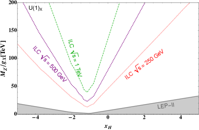
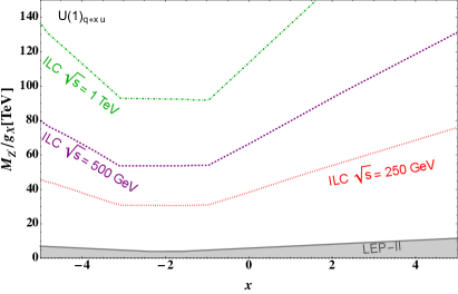
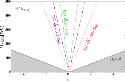
Figure 1: Current LEP-II bounds(grey-shaded, ruled out) on $M_{Z^{\prime}}/g_{X}$ of the $U(1)$ theories for different general $U(1)$ charges and the future ILC projections for $\sqrt{s}=250$ GeV (red), $500$ GeV (purple) and $1$ TeV (green) respectively at 95$\%$ C.L.

Machine	$\sqrt{s}$	95% CL lower limit on the $M_{Z^{\prime}}/g_{X}$ of U$(1)_{X}$ scenario (in TeV)
		$x_{H}=-2$	$x_{H}=-1$	$x_{H}=-0.5$	$x_{H}=0$	$x_{H}=0.5$	$x_{H}=1$	$x_{H}=2$
LEP-II	209 GeV	5.0	2.2	4.4	7.0	10.3	11.1	18.0
ILC	250 GeV	31.6	16.3	29.5	48.2	64.3	79.0	113.7
	500 GeV	54.4	26.3	50.1	81.6	110.2	139.1	199.7
	1 TeV	88.6	47.7	84.8	137.2	185.8	238.2	339.2
		95% CL lower limit on the $M_{Z^{\prime}}/g_{X}$ of U$(1)_{xq-\tau_{R}^{3}}$ scenario (in TeV)
		$x=-2$	$x=0$	$x=\frac{1}{3}$	$x=0.25$	$x=0.5$	$x=\frac{1}{6}$	$x=2$
LEP-II	209 GeV	60.3	5.0	7.0	4.4	11.1	2.2	56.6
ILC	250 GeV	415.9	31.6	48.2	29.5	ds79.0	16.3	378.0
	500 GeV	728.7	54.4	81.6	50.1	139.1	26.3	673.1
	1 TeV	1272.6	88.6	137.2	84.8	238.2	47.7	1163.4
		95% CL lower limit on the VEV of U$(1)_{q+xu}$ scenario (in TeV)
		$x=-2$	$x=-1$	$x=-0.5$	$x=0$	$x=0.5$	$x=1$	$x=2$
LEP-II	209 GeV	3.2	4.2	4.65	5.4	5.9	7.0	7.4
ILC	250 GeV	30.3	30.2	33.8	37.5	41.5	48.2	53.5
	500 GeV	53.1	53.4	59.8	66.5	72.1	81.6	93.2
	1 TeV	92.6	91.1	101.9	114.0	124.3	137.2	158.0

Table 2: The $95\%$ CL lower limits on VEV in the general $U(1)$ extensions of SM model from $e^{+}e^{-}\to f\bar{f}$ processes for different charges recasting the limits on the effective scale of contact interactions from [172, 174]. We show the strongest limit out of all the different channels considered in the $e^{-}e^{+}\to f\overline{f}$ process for $M_{Z^{\prime}}\gg\sqrt{s}$.

II.2 Flavored scenarios

We consider the generation dependent coupling with $Z^{\prime}$ in this section unlike the previous section. There are two scenarios under consideration: (i) leptophilic scenarios, commonly known as $L_{i}-L_{j}$ scenarios and (ii) $B-3L_{i}$ where quarks are charged under the additional $U(1)$ gauge group, however, $i$th generation lepton will be charged under $U(1)_{B-3L_{i}}$ gauge group:

• Apart from the flavor independent anomaly free scenarios, there also appear a variety of flavor dependent scenarios which are anomaly free, too. We find gauged $L_{e}-L_{\mu}$, $L_{e}-L_{\tau}$ and $L_{\mu}-L_{\tau}$ such scenarios. In these cases a $Z^{\prime}$ boson is originated after the spontaneously broken $U(1)_{L_{i}-L_{j}}$ symmetry [23, 24, 25]. In this case under U(1)${}_{L_{i}-L_{j}}$ gauge group charged leptons $L_{i}$ is positive and $L_{j}$ is negative respectively. The RHNs also follow the same path of charged leptons. The remaining generation of the charged leptons and RHNs are uncharged under $U(1)_{L_{i}-L_{j}}$ gauge group. The quarks are uncharged under the $U(1)_{L_{i}-L_{j}}$ symmetry.

  Fields	$SU(3)_{c}\otimes SU(2)_{L}\otimes U(1)_{Y}$	$U(1)_{L_{e}-L_{\mu}}$	$U(1)_{L_{\tau}-L_{e}}$	$U(1)_{L_{\mu}-L_{\tau}}$
  $q_{L}^{i}$	$(3,2,\frac{1}{6})$	0	0	0
  $u_{R}^{i}$	$(3,1,\frac{2}{3})$	0	0	0
  $d_{R}^{i}$	$(3,1,-\frac{1}{3})$	0	0	0
  $\ell_{L}^{i}$	$(1,2,-\frac{1}{2})$	$\{1,-1,0\}$	$\{-1,0,1\}$	$\{0,1,-1\}$
  $e_{R}^{i}$	$(1,1,-1)$	$\{1,-1,0\}$	$\{-1,0,1\}$	$\{0,1,-1\}$
  $H$	$(1,2,-\frac{1}{2})$	0	0	0
  $N^{j}$	$(1,1,0)$	$\{1,-1,0\}$	$\{-1,0,1\}$	$\{0,1,-1\}$
  $\Phi$	$(1,1,0)$	$-2$	$-2$	$-2$

  Table 3: Particle content and charge assignments for the $U(1)_{L_{i}-L_{j}}$ models. Two new SM singlet fields $N$ (fermion) and $\Phi$ (scalar) are added to the SM particle content where ${i,j}$ are the flavour indices for three generations.

  Inclusion of the RHNs allows to reproduce lepton mixing without charged lepton flavor changing couplings under $U(1)_{L_{i}-L_{j}}$ being phenomenologically viable. The particle content of the scenarios are given in Tab. 3.

  The Yukawa interaction in $L_{i}-L_{j}$ scenario following the particle content given in Tab. 3 can be written as

  $${\cal L}^{\rm Yukawa} = -Y_{u}^{\alpha\beta}\overline{q_{L}^{\alpha}}Hu_{R}^{\beta}-Y_{d}^{\alpha\beta}\overline{q_{L}^{\alpha}}\tilde{H}d_{R}^{\beta}-Y_{e}^{\alpha\beta}\overline{\ell_{L}^{\alpha}}\tilde{H}e_{R}^{\beta}-Y_{\nu}^{i}\overline{\ell_{L}^{i}}HN_{R}^{i}-Y_{\nu}^{j}\overline{\ell_{L}^{j}}HN_{R}^{j}$$ (17)

  $$-Y_{N}^{i}\Phi\overline{(N_{R}^{i})^{c}}N_{R}^{i}-Y_{N}^{j}\Phi^{*}\overline{(N_{R}^{j})^{c}}N_{R}^{j}-Y_{\nu}^{k}\overline{\ell_{L}^{k}}HN_{R}^{k}+{\rm h.c.}-M_{N}^{k}\overline{{N_{R}^{k}}^{c}}N_{R}^{k}-M_{N}^{ij}\overline{{N_{R}^{i}}^{c}}N_{R}^{j}$$

  where $\alpha,\beta$ denote three generations, $i,~{}j$ denote the corresponding $i$th and $j$th generations of leptons with $k\neq i\neq j$. The renormalizable scalar potential can be written as

  $$V\ =\ m_{h}^{2}(H^{\dagger}H)+\lambda_{H}(H^{\dagger}H)^{2}+m_{\Phi}^{2}(\Phi^{\dagger}\Phi)+\lambda_{\Phi}(\Phi^{\dagger}\Phi)^{2}+\lambda^{\prime}(H^{\dagger}H)(\Phi^{\dagger}\Phi)~{},$$ (18)

  where $H$ is the SM Higgs doublet and $\Phi$ is the SM-singlet scalar fields where we can approximate $\lambda^{\prime}$ to be very small. After breaking the $U(1)_{L_{i}-L_{j}}$ gauge and electroweak symmetries, the scalar fields $H$ and $\Phi$ develop their vacuum expectation values (VEVs) in the similar fashion given in Eq. 5 and at the potential minimum the electroweak scale is demarcated as $v=246$ GeV and $v_{\Phi}$ is taken to be a free parameter. After the breaking of the general $U(1)_{L_{i}-L_{j}}$ symmetry under a limit $v_{\Phi}\gg v$, the mass of the $Z^{\prime}$ can be written as

  $$M_{Z^{\prime}}=2g_{X}v_{\Phi}~{}.$$ (19)

  which is a free parameter. Here $g_{X}$ is the $U(1)_{L_{i}-L_{j}}$ coupling considered for the cases shown in Tab. 3. From the Yukawa interactions given in Eq. 2, we find that the RHNs interact with the SM-singlet scalar field $\Phi$. This Yukawa interaction generates Majorana mass term for heavy neutrinos after the $U(1)_{L_{i}-L_{j}}$ symmetry is broken. After the electroweak symmetry breaking, the Dirac mass term is generated from the interaction term among the SM like Higgs doublet, SM lepton doublet and the SM-singlet RHN. There is also a Majorana mass term for the RHNs with $k\neq i,~{}j$. The Dirac and Majorana mass terms can be written as

  $$\tilde{m}_{D}^{i(j)\neq k}=\frac{Y_{\nu}^{i(j)\neq k}}{\sqrt{2}}v,\quad\tilde{m}_{N}^{i(j)}=\frac{Y_{N}^{i(j)}}{\sqrt{2}}v_{\Phi}\,.$$ (20)

  Tiny neutrino mass and flavor mixing can be generated using

  $$m_{D}\equiv\tilde{m}_{D}^{i}\bigoplus\tilde{m}_{D}^{j}\bigoplus\tilde{m}_{D}^{k}\quad\text{and}\quad m_{N}\equiv\tilde{m}_{N}^{i}\bigoplus\tilde{m}_{N}^{j}\bigoplus M_{N}^{k}$$

  through the seesaw mechanism. Neutrino mass generation mechanism is not the main motivation of this paper therefore we skip detailed discussions on flavor structure of this scenario. The interaction Lagrangian between $Z^{\prime}$ and SM leptons can be written as

  $$\mathcal{L}^{f}=-g_{X}(\overline{f_{L}^{i}}\gamma^{\mu}f_{L}^{i}+\overline{f_{R}^{i}}\gamma^{\mu}f_{R}^{i}-\overline{f_{L}^{j}}\gamma^{\mu}f_{L}^{j}-\overline{f_{R}^{j}}\gamma^{\mu}f_{R}^{j})Z_{\mu}^{\prime}~{},$$ (21)

  where $f^{i(j)}$ includes $i(j)$th generation SM leptons with $i\neq j$. Hence, we calculate the partial decay widths of $Z^{\prime}$ into the corresponding SM leptons following Eq. 10 and using $q_{L,R}^{i}=1$, $q_{L,R}^{j}=-1$ according to Tab. 3 as

  $$\Gamma(Z^{\prime}\to\bar{\ell^{i(j)}}\ell^{i(j)}) =\frac{M_{Z^{\prime}}g_{X}^{2}}{12\pi}\left[\left(1-\frac{m_{f}^{2}}{M_{Z^{\prime}}^{2}}\right)+3\frac{m_{f}^{2}}{M_{Z^{\prime}}^{2}}\right]~{},$$ (22)

  where $m_{f}$ is the mass of SM leptons. The partial decay width of the $Z^{\prime}$ into a pair of light neutrinos of single generation can be written as following Eq. 11 and setting $q_{L}^{i}=1$ and $q_{L}^{j}=-1$ from Tab. 3

  $$\Gamma(Z^{\prime}\to\nu^{i(j)}\nu^{i(j)})=\frac{M_{Z^{\prime}}g_{X}^{2}}{24\pi}~{},$$ (23)

  where we neglect the effect of tiny neutrino mass. Like a general $U(1)$ extended SM scenario, the $Z^{\prime}$ gauge boson decays into a pair of heavy Majorana neutrinos can be inferred from Eq. 12 by putting $q_{N_{R}}^{i}=1$ and $q_{N_{R}}^{j}=-1$. Hence the corresponding partial decay width for a single generation of the heavy neutrino pair is

  $$\Gamma(Z^{\prime}\to N_{R}^{i(j)}N_{R}^{i(j)})=\frac{M_{Z^{\prime}}g_{X}^{2}}{24\pi}\left(1-\frac{4M_{N}^{2}}{M_{Z^{\prime}}^{2}}\right)^{\frac{3}{2}}$$ (24)

  with $M_{N}$ being the corresponding heavy neutrino mass. In this scenario, $Z^{\prime}$ has no direct coupling with the SM quarks allowing its dominant decay into lepton pairs. Hence we can calculate the total decay width of $Z^{\prime}$ in $L_{i}-L_{j}$ scenario. In this paper we consider flavor conserving $Z^{\prime}$ couplings. Following Eqs. 14-16, we estimate the LEP-II constraint on $L_{e}-L_{\mu}$ and $L_{\tau}-L_{e}$ as $M_{Z^{\prime}}/g_{X}>7$ TeV comparing the limits on the effective scales from [172] using $e^{-}e^{+}\to f\bar{f}$ process for $M_{Z^{\prime}}\gg\sqrt{s}$ satisfying large VEV approximation. The prospective limits at 250 GeV, 500 GeV and 1 TeV ILC in the context of these scenarios will be $M_{Z^{\prime}}/g_{X}>48.2$ TeV, $81.6$ TeV and $137.2$ TeV respectively. Due to model structure under our consideration, $e^{-}e^{+}\to f\bar{f}$ process can not constrain $L_{\mu}-L_{\tau}$ scenario because electron positron has no direct coupling with $Z^{\prime}$.

• There is another type of flavored scenario namely $B-3L_{i}$ where one of the three generations of the $\ell_{L}^{i}$ and $e_{R}^{i}$ will be charged under the additional abelian gauge group while the rest of the two generations are not. The particle content is given in Tab. 4. The RHNs being SM-singlet in this scenario follow the same footprints of the charged leptons. If the first generation of $\ell_{L}^{i}$ and $e_{R}^{i}$ are charged under $U(1)_{B-3L_{i}}$ then the first generation of $N^{j}$ will be charged under this gauge group and second and third generations of these fermions will not be charged. The inclusion of the three generations of the RHNs makes the model free from gauge and mixed gauge-gravity anomalies. Under this gauge group SM Higgs is uncharged. The quarks in the model have charge $\frac{1}{3}$ under $U(1)_{B-3L_{i}}$ gauge group.

  Fields	$SU(3)_{c}\otimes SU(2)_{L}\otimes U(1)_{Y}$	$U(1)_{B-3L_{e}}$	$U(1)_{B-3L_{\mu}}$	$U(1)_{B-3L_{\tau}}$
  $q_{L}^{i}$	$(3,2,\frac{1}{6})$	$\frac{1}{3}$	$\frac{1}{3}$	$\frac{1}{3}$
  $u_{R}^{i}$	$(3,1,\frac{2}{3})$	$\frac{1}{3}$	$\frac{1}{3}$	$\frac{1}{3}$
  $d_{R}^{i}$	$(3,1,-\frac{1}{3})$	$\frac{1}{3}$	$\frac{1}{3}$	$\frac{1}{3}$
  $\ell_{L}^{i}$	$(1,2,-\frac{1}{2})$	{-3,0,0}	{0,-3,0}	{0,0,-3}
  $e_{R}^{i}$	$(1,1,-1)$	{-3,0,0}	{0,-3,0}	{0,0,-3}
  $H$	$(1,2,-\frac{1}{2})$	0	0	0
  $N^{i}$	$(1,1,0)$	{-3,0,0}	{0,-3,0}	{0,0,-3}
  $\Phi$	$(1,1,0)$	6	6	6

  Table 4: Particle content and charge assignments for the $U(1)_{B-3L_{i}}$ models. Two new SM singlet fields $N$ (fermion) and $\Phi$ (scalar) are added to the SM particle content where ${i,j}$ are the flavour indices for three generations.

  An SM singlet scalar $\Phi$ can be introduced in this scenario which is charged under the $U(1)_{B-3L_{i}}$ gauge group, and can generate the Majorana mass term for the RHNs. The Yukawa interaction for the particle content given in Tab. 4 can be written as

  $${\cal L}^{\rm Yukawa} = -Y_{u}^{\alpha\beta}\overline{q_{L}^{\alpha}}Hu_{R}^{\beta}-Y_{d}^{\alpha\beta}\overline{q_{L}^{\alpha}}\tilde{H}d_{R}^{\beta}-Y_{e}^{\alpha\beta}\overline{\ell_{L}^{\alpha}}\tilde{H}e_{R}^{\beta}-\sum_{\alpha\neq i}\sum_{\beta\neq i}Y_{\nu}^{\alpha\beta}\overline{\ell_{L}^{\alpha}}HN_{R}^{\beta}-Y_{\nu}^{ii}\overline{\ell_{L}^{i}}HN_{R}^{i}$$ (25)

  $$-Y_{N}^{ii}\Phi\overline{(N_{R}^{i})^{c}}N_{R}^{i}+{\rm h.c.}-\sum_{j\neq i}\tilde{M}_{N}^{jj}\overline{(N_{R}^{j})^{c}}N_{R}^{j}~{}~{}~{}~{}~{}~{}~{}$$

  Now, following $U(1)_{B-3L_{i}}$ and the electroweak symmetry breaking, we find the Dirac and Majorana masses of the neutrinos

  $$\tilde{m}_{D}^{\alpha\beta}=\frac{Y_{\nu}^{\alpha\beta}v}{\sqrt{2}},\;\;\tilde{m}_{D}^{ii}=\frac{Y_{\nu}^{ii}v}{\sqrt{2}}\;\;\text{and}\;\;\tilde{m}_{N}^{ii}=\frac{Y_{N}^{ii}v_{\Phi}}{\sqrt{2}}.$$ (26)

  Using $m_{D}\equiv\tilde{m}_{D}^{\alpha\beta}\bigoplus\tilde{m}_{D}^{ii}$ and $m_{N}=\tilde{m}_{N}^{ii}\bigoplus\tilde{M}_{N}^{jj}$ and following the line of Eq. 8, we find that the light neutrino mass can be generated by the seesaw mechanism resulting flavor mixing. The neutrino mass generation mechanism is not the main motivation of this paper, therefore, we skip detailed discussions on flavor structure of this scenario. The scalar potential of this scenario is given exactly by Eq. 18. Following Eq. 5 and the scalar kinetic term we obtain the $Z^{\prime}$ mass assuming $v_{\Phi}\gg v$

  $$M_{Z^{\prime}}=6g_{X}v_{\Phi}.$$ (27)

  The interaction Lagrangian between $Z^{\prime}$ and SM leptons can be written as

  $$\mathcal{L}^{f}=-g_{X}(\overline{q_{L}^{i}}\gamma^{\mu}Q_{L}^{q}q_{L}^{i}+\overline{q_{R}^{i}}\gamma^{\mu}Q_{R}^{q}q_{R}^{i}+\overline{f_{L}^{i}}\gamma^{\mu}Q_{L}^{\ell^{i}}f_{L}^{i}+\overline{f_{R}^{i}}\gamma^{\mu}Q_{R}^{\ell^{i}}f_{R}^{i})Z_{\mu}^{\prime}~{}$$ (28)

  where $Q_{L(R)}^{q}$ is left (right) handed charged of the quarks under $U(1)_{B-3L_{i}}$ scenario whereas $Q_{L(R)}^{\ell^{i}}$ is the $U(1)_{B-3L_{i}}$ charge of $i$th generation left (right) handed SM lepton according to Tab. 4. The partial decay width of the $Z^{\prime}$ can be written following Eq. 10 where we write the corresponding charges for the quarks and leptons from Tab. 4. To calculate $\Gamma(Z^{\prime}\to q\bar{q})$, we consider all the left and right-handed flavors, so that it can be written as

  $$\Gamma(Z^{\prime}\to q\bar{q})=\frac{M_{Z^{\prime}}g_{X}^{2}}{36\pi}\left[\left(1-\frac{m_{q}^{2}}{M_{Z^{\prime}}^{2}}\right)+3\frac{m_{q}^{2}}{M_{Z^{\prime}}^{2}}\right]~{},$$ (29)

  where $m_{q}$ is the corresponding quark mass. In this scenario only one generation of the leptons is charged under the $U(1)_{B-3L_{i}}$ gauge group. Hence we derive the partial decay width of $Z^{\prime}$ charged leptons $({\ell^{i}}^{\pm})$, light neutrinos $(\nu^{i})$ and heavy neutrinos $(N^{i})$ as

  $$\Gamma(Z^{\prime}\to\bar{\ell^{i}}\ell^{i}) = \frac{3M_{Z^{\prime}}g_{X}^{2}}{4\pi}\left[\left(1-\frac{m_{f}^{2}}{M_{Z^{\prime}}^{2}}\right)+3\frac{m_{f}^{2}}{M_{Z^{\prime}}^{2}}\right]$$

  $$\Gamma(Z^{\prime}\to\nu^{i}\nu^{i}) = \frac{3M_{Z^{\prime}}g_{X}^{2}}{8\pi}$$

  $$\Gamma(Z^{\prime}\to N_{R}^{i}N_{R}^{i}) = \frac{3M_{Z^{\prime}}g_{X}^{2}}{8\pi}\left(1-\frac{4{M_{N}^{i}}^{2}}{M_{Z^{\prime}}^{2}}\right)^{\frac{3}{2}}$$ (30)

  respectively. Hence we find that $Z^{\prime}$ dominantly decays into leptons in the case of $B-3L_{i}$ scenario. The constraint on $B-3L_{e}$ scenario from LEP-II can be obtained as $M_{Z^{\prime}}/g_{X}>2.33$ TeV comparing the limits on the effective scales from [172] using $e^{-}e^{+}\to f\bar{f}$ process for $M_{Z^{\prime}}>>\sqrt{s}$ following Eqs. 14-16. Following the same manner prospective bounds at the $250$ GeV, $500$ GeV and $1$ TeV ILC can be estimated $M_{Z^{\prime}}/g_{X}>$ 16.07 TeV, 27.20 TeV and 45.73 TeV respectively. $B-3L_{\mu}$ and $B-3L_{\tau}$ scenarios can not be constrained using LEP-II results from $e^{-}e^{+}\to f\bar{f}$ process because $e^{\pm}$ has no direct coupling with $Z^{\prime}$ in these cases.

III Theory of neutrino heating

In the general $U(1)$ extended and flavored scenarios we found that neutrinos can interact with the electrons. As a result of the influence of the additional $U(1)$ extension of the SM, the neutrinos interact with the electron through SM propagators including $W$, $Z$ bosons and neutral BSM gauge bosons $Z^{\prime}$ as shown in Fig. 2. For $\nu_{e}$ we have $W$, $Z$ and $Z^{\prime}$ mediated $s,~{}t-$channel processes whereas for $\nu_{\mu,\tau}$ only $Z$ and $Z^{\prime}$ mediated $s-$channnel processes will participate. We also include corresponding interference between the channels. Due to the presence of $Z^{\prime}$, the couplings of neutrino and electron with $Z^{\prime}$ will carry the general $U(1)$ charges which will be manifested in the analysis. Similarly the flavored scenarios can also show such interactions depending on the flavor structure. As a result we study such scenarios in the light of GRB to probe the effect of the $Z^{\prime}$ gauge boson by constraining the plane of the additional $U(1)$ coupling and $Z^{\prime}$ mass and compare them with existing bounds.

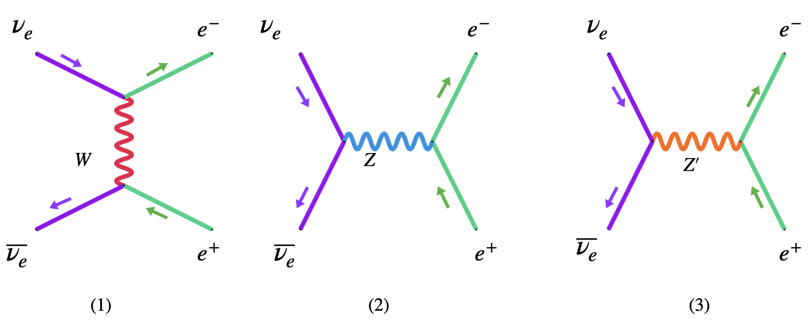
Figure 2: Neutrino anti-neutrino scattering processes in SM and BSM scenario induced by $Z^{\prime}$ gauge boson. The $\nu_{e}\bar{\nu}_{e}\to e^{-}e^{+}$ process involves all three contributions from SM $(W,~{}Z)$ and BSM $(Z^{\prime})$ processes whereas $\nu_{\mu,\tau}\bar{\nu}_{\mu,\tau}\to e^{-}e^{+}$ process involves contributions from $Z$ and $Z^{\prime}$ bosons respectively. The $Z^{\prime}$ interaction depends on the model structure and corresponding $U(1)$ charges.

In the context of a general $U(1)_{X}$ scenario from Fig. 2 we study the $\nu_{e}\bar{\nu}_{e}\rightarrow e^{+}e^{-}$ process and calculate

$$\{\sigma(\nu_{e}\bar{\nu}_{e} \rightarrow e^{+}e^{-})\}=\left\{\frac{G_{F}^{2}}{3\pi}(1+4\sin^{2}\theta_{w}+8\sin^{4}\theta_{w})+\frac{g_{X}^{4}}{6\pi M_{Z^{\prime}}^{4}}\left(\frac{x_{H}}{2}+x_{\Phi}\right)^{2}\left[\left(\frac{x_{H}}{2}+x_{\Phi}\right)^{2}+(x_{H}+x_{\Phi})^{2}\right]+\right.$$

$$\left.\frac{4G_{F}g_{X}^{2}}{3\sqrt{2}\pi M_{Z^{\prime}}^{2}}\left(\frac{x_{H}}{2}+x_{\Phi}\right)\left[\sin^{2}\theta_{w}\left(\frac{3x_{H}}{2}+2x_{\Phi}\right)-\frac{1}{2}\left(\frac{x_{H}}{2}+x_{\Phi}\right)\right]+\frac{4G_{F}g_{X}^{2}}{3\sqrt{2}\pi M_{Z^{\prime}}^{2}}\left(\frac{x_{H}}{2}+x_{\Phi}\right)^{2}\right\}(E_{\nu}E_{\bar{\nu}}-\vec{p}_{\nu}.\vec{p}_{\bar{\nu}})^{2}$$ (31)

where the first term corresponds to the SM process mediated by the $W$ and $Z$ bosons and the second term corresponds to the $Z^{\prime}$ mediated process, respectively. The interference between the $Z$ and $Z^{\prime}$ mediated processes is represented by the third term, and the fourth term represents the interference between $W$ and $Z^{\prime}$ mediated processes. Similarly from $\nu_{\mu/\tau}\bar{\nu}_{\mu/\tau}\rightarrow e^{+}e^{-}$ process through the $Z$ and $Z^{\prime}$ channels we calculate

$$\{\sigma(\nu_{\mu/\tau}\bar{\nu}_{\mu/\tau} \rightarrow e^{+}e^{-})\}=\left\{\frac{G_{F}^{2}}{3\pi}(1-4\sin^{2}\theta_{w}+8\sin^{4}\theta_{w})+\frac{g_{X}^{4}}{6\pi M_{Z^{\prime}}^{4}}\left(\frac{x_{H}}{2}+x_{\Phi}\right)^{2}\left[\left(\frac{x_{H}}{2}+x_{\Phi}\right)^{2}+(x_{H}+x_{\Phi})^{2}\right]+\right.$$

$$\left.\frac{4G_{F}g_{X}^{2}}{3\sqrt{2}\pi M_{Z^{\prime}}^{2}}\left(\frac{x_{H}}{2}+x_{\Phi}\right)\left[\sin^{2}\theta_{w}\left(\frac{3x_{H}}{2}+2x_{\Phi}\right)-\frac{1}{2}\left(\frac{x_{H}}{2}+x_{\Phi}\right)\right]\right\}(E_{\nu}E_{\bar{\nu}}-\vec{p}_{\nu}.\vec{p}_{\bar{\nu}})^{2}\,,$$ (32)

where the first term involves the SM process mediated by the $Z$ boson, the second term stands for the $Z^{\prime}$ mediated process, and the third term stands for the interference between the $Z$ and $Z^{\prime}$. In these expressions, $\theta_{w}$ stands for the Weinberg angle. In this analysis we consider $\sin^{2}\theta_{w}=0.23121$ which estimates $(1+4\sin^{2}\theta_{w}+8\sin^{4}\theta_{w})=2.3525$ and $(1-4\sin^{2}\theta_{w}+8\sin^{4}\theta_{w})=0.592825$ respectively. The Fermi constant is $G_{F}=1.663787\times 10^{-5}$ GeV^-2 [1].

The $\nu\bar{\nu}\to e^{+}e^{-}$ process can be studied in the context of the other two $U(1)$ extensions. First we consider $U(1)_{xq-\tau_{R}^{3}}$ model where we calculate the contribution from $\nu_{e}\bar{\nu}_{e}\to e^{+}e^{-}$ process

$$\{\sigma(\nu_{e}\bar{\nu}_{e}\rightarrow e^{+}e^{-})\} = \Big{[}\frac{G_{F}^{2}}{3\pi}(1+4\sin^{2}\theta_{w}+8\sin^{4}\theta_{w})+\frac{g_{X}^{4}9x^{2}}{6\pi M_{Z^{\prime}}^{4}}\{9x^{2}+(1-6x)^{2}\}+$$

$$\frac{4g_{X}^{2}G_{F}}{3\sqrt{2}\pi M_{Z^{\prime}}^{2}}(-3x)\left\{(-3x)\left(-\frac{1}{2}+\sin^{2}\theta_{w}\right)+(1-6x)\sin^{2}\theta_{w}\right\}+\frac{4g_{X}^{2}G_{F}}{3\sqrt{2}\pi M_{Z^{\prime}}^{2}}9x^{2}\Big{]}(E_{\nu}E_{\bar{\nu}}-\vec{p}_{\nu}.\vec{p}_{\bar{\nu}})^{2}$$

and the contribution from $\nu_{\mu,\tau}\bar{\nu}_{\mu,\tau}\to e^{+}e^{-}$ process can be calculated as

$$\{\sigma(\nu_{\mu/\tau}\bar{\nu}_{\mu/\tau}\rightarrow e^{+}e^{-})\} = \Big{[}\frac{G_{F}^{2}}{3\pi}(1-4\sin^{2}\theta_{w}+8\sin^{4}\theta_{w})+\frac{g_{X}^{4}9x^{2}}{6\pi M_{Z^{\prime}}^{4}}\{9x^{2}+(1-6x)^{2}\}+$$ (34)

$$\frac{4g_{X}^{2}G_{F}}{3\sqrt{2}\pi M_{Z^{\prime}}^{2}}(-3x)\left\{(-3x)\left(-\frac{1}{2}+\sin^{2}\theta_{w}\right)+(1-6x)\sin^{2}\theta_{w}\right\}\Big{]}(E_{\nu}E_{\bar{\nu}}-\vec{p}_{\nu}.\vec{p}_{\bar{\nu}})^{2}$$

Now we consider $U(1)_{q+xu}$ model where we calculate the contribution from $\nu_{e}\bar{\nu}_{e}\to e^{+}e^{-}$ process

$$\{\sigma(\nu_{e}\bar{\nu}_{e}\rightarrow e^{+}e^{-})\} = \Big{[}\frac{G_{F}^{2}}{3\pi}(1+4\sin^{2}\theta_{w}+8\sin^{4}\theta_{w})+\frac{g_{X}^{4}}{6\pi M_{Z^{\prime}}^{4}}\left(1+\frac{(2+x)^{2}}{9}\right)+\frac{4g_{X}^{2}G_{F}}{3\sqrt{2}\pi M_{Z^{\prime}}^{2}}\left\{\left(-\frac{1}{2}+\sin^{2}\theta_{w}\right)+\right.$$ (35)

$$\left.\frac{(2+x)}{3}\sin^{2}\theta_{w}\right\}+\frac{4g_{X}^{2}G_{F}}{3\sqrt{2}\pi M_{Z^{\prime}}^{2}}\Big{]}(E_{\nu}E_{\bar{\nu}}-\vec{p}_{\nu}.\vec{p}_{\bar{\nu}})^{2}$$

and the contribution from $\nu_{\mu,\tau}\bar{\nu}_{\mu,\tau}\to e^{+}e^{-}$ process can be calculated as

$$\{\sigma(\nu_{\mu/\tau}\bar{\nu}_{\mu/\tau}\rightarrow e^{+}e^{-})\} = \Big{[}\frac{G_{F}^{2}}{3\pi}(1-4\sin^{2}\theta_{w}+8\sin^{4}\theta_{w})+\frac{g_{X}^{4}}{6\pi M_{Z^{\prime}}^{4}}\left\{1+\frac{(2+x)^{2}}{9}\right\}+\frac{4g_{X}^{2}G_{F}}{3\sqrt{2}\pi M_{Z^{\prime}}^{2}}\left\{\left(-\frac{1}{2}+\sin^{2}\theta_{w}\right)+\right.$$ (36)

$$\left.\frac{(2+x)}{3}\sin^{2}\theta_{w}\right\}\Big{]}(E_{\nu}E_{\bar{\nu}}-\vec{p}_{\nu}.\vec{p}_{\bar{\nu}})^{2}$$

We study the $L_{i}-L_{j}$ scenarios where $L_{e}-L_{\mu}$ and $L_{e}-L_{\tau}$ models manifest the interaction between the $Z^{\prime}$ and the first generation of lepton. In the context of $L_{e}-L_{\mu}$ model the contribution from the $\nu_{e}\bar{\nu}_{e}\to e^{+}e^{-}$ process is given by

$$\{\sigma(\nu_{e}\bar{\nu}_{e}\to e^{-}e^{+})\} = \Big{[}\frac{G_{F}^{2}}{3\pi}(1+4\sin^{2}\theta_{w}+8\sin^{4}\theta_{w})+\frac{g_{X}^{4}}{3\pi M_{Z^{\prime}}^{4}}+\frac{4G_{F}g_{X}^{4}}{3\sqrt{2}\pi M_{Z^{\prime}}^{2}}\left(-\frac{1}{2}+2\sin^{2}\theta_{w}\right)+$$ (37)

$$\frac{4G_{F}}{3\sqrt{2}\pi}\frac{g_{X}^{2}}{M_{Z^{\prime}}^{2}}\Big{]}(E_{\nu}E_{\bar{\nu}}-\vec{p}_{\nu}.\vec{p}_{\bar{v}})^{2}$$

where the first term stands for the $t$-channel and $s$-channel $W$, $Z$ mediated process of the SM, the second term stands for the $s$ channel $Z^{\prime}$ mediated process, the third term stands for the interference between the $Z$ and $Z^{\prime}$ mediated processes and finally, the fourth term represents the interference between the $W$ and $Z^{\prime}$ mediated processes, respectively. The contribution from the $\nu_{\mu}\bar{\nu}_{\mu}\to e^{+}e^{-}$ process can be written as

$$\{\sigma(\nu_{\mu}\bar{\nu}_{\mu}\to e^{-}e^{+})\}=\Big{[}\frac{G_{F}^{2}}{3\pi}(1-4\sin^{2}\theta_{w}+8\sin^{4}\theta_{w})+\frac{g_{X}^{4}}{3\pi M_{Z^{\prime}}^{4}}-\frac{4G_{F}g_{X}^{2}}{3\sqrt{s}\pi M_{Z^{\prime}}^{2}}\left(-\frac{1}{2}+2\sin^{2}\theta_{w}\right)\Big{]}(E_{\nu}E_{\bar{\nu}}-\vec{p}_{\nu}.\vec{p}_{\bar{v}})^{2}$$ (38)

where the first term corresponds to the $s$-channel $Z$ mediated process, the second term corresponds to the $Z^{\prime}$ mediated $s$ channel process and the third term represents the interference between $Z$ and $Z^{\prime}$ mediated processes, respectively. We find that in the context of $L_{e}-L_{\tau}$ scenario the $\nu_{e}\bar{\nu}_{e}\to e^{+}e^{-}$ process will contribute in the same way as it has been given in Eq. 37. Similarly $\nu_{\tau}\bar{\nu}_{\tau}\to e^{+}e^{-}$ process will contribute in the same way as given in Eq. 38. In the $L_{\mu}-L_{\tau}$ scenario there is no direct interaction between electron and $Z^{\prime}$, however, the introduction of the kinetic mixing between $Z$ and $Z^{\prime}$ could make $\nu_{\mu,\tau}\bar{\nu}_{\mu,\tau}\to e^{-}e^{+}$ a process possible. The kinetic mixing and higher order processes at quantum level are not the motivations of this paper, which restricts us to discuss the $L_{\mu}-L_{\tau}$ model.

Studying the $B-3L_{i}$ scenarios we find that only the $B-3L_{e}$ counterpart of this class of models contributes to the $\nu\nu\to e^{+}e^{-}$ process where only $\nu_{e}$ flavor will contribute to the BSM process due to the $U(1)_{B-3L{e}}$ gauge charge. The cross-section for the $\nu{\bar{\nu}}\to e^{+}e^{-}$ process in $B-3L_{\mu}$ and $B-3L_{\tau}$ cases will be exactly the same as the SM due to the fact that we do not consider gauge kinetic mixing. Finally, in the case of $B-3L_{e}$, we obtain

$$\{\sigma(\nu_{e}\bar{\nu}_{e}\to e^{-}e^{+})\}=\Big{[}\frac{G_{F}^{2}}{3\pi}(1+4\sin^{2}\theta_{W}+8\sin^{4}\theta_{W})+\frac{27g_{X}^{4}}{\pi M_{Z^{\prime}}^{4}}+\frac{12G_{F}g_{X}^{2}}{\sqrt{2}\pi M_{Z^{\prime}}^{2}}(-\frac{1}{2}+2\sin^{2}\theta_{w})+\frac{12G_{F}g_{X}^{2}}{\sqrt{2}\pi M_{Z^{\prime}}^{2}}\Big{]}(E_{\nu}E_{\bar{\nu}}-\vec{p}_{\nu}.\vec{p}_{\bar{v}})^{2}$$ (39)

where the first term shows the SM contribution, the second term stands for the $s$ channel $Z^{\prime}$ mediated process, the thirst term represents the interference between $Z$ and $Z^{\prime}$, whereas the fourth term represents the interference between $Z^{\prime}$ and $W$ bosons, respectively.

III.1 Neutrino Trajectory in a general metric

The line element in a general space-time metric with an off-diagonal $t\phi$ element is given by

$$ds^{2}=g_{tt}\;dt^{2}+g_{rr}\;dr^{2}+g_{\theta\theta}\;d\theta^{2}+g_{\phi\phi}\;d\phi^{2}+2g_{t\phi}\;dt\;d\phi$$ (40)

Since neutrinos are extremely light, for simplicity, we consider them as massless particles. We also restrict the dynamics to a plane with $\theta=\pi/2$ . The null geodesic equation for a massless particle is then given by

$$g_{tt}\;\dot{t}^{2}+g_{rr}\;\dot{r}^{2}+g_{\phi\phi}\;\dot{\phi}^{2}+2g_{t\phi}\;\dot{\phi}\dot{t}=0$$ (41)

The Lagrangian of a massless particle is given by $\mathcal{L}=\frac{1}{2}g_{\mu\nu}\dot{x}^{\mu}\dot{x}^{\nu}$ and the generalized momenta can be derived as follows,

$$p_{t}=\frac{\partial\mathcal{L}}{\partial\dot{t}}=g_{tt}\;\dot{t}+g_{t\phi}\;\dot{\phi}=-E,\;\;p_{r}=\frac{\partial\mathcal{L}}{\partial\dot{r}}=g_{rr}\;\dot{r},\;\;p_{\phi}=\frac{\partial\mathcal{L}}{\partial\dot{\phi}}=g_{\phi\phi}\;\dot{\phi}+g_{t\phi}\;\dot{t}=L$$ (42)

where $E$ and $L$ are the energy and angular momentum of the neutrino. Eq. 42 can be simultaneously solved to obtain $\dot{\phi}$ and $\dot{t}$ as

$$\dot{t}=\frac{L\;g_{t\phi}+E\;g_{\phi\phi}}{g_{t\phi}^{2}-g_{tt}\;g_{\phi\phi}},\;\;\;\dot{\phi}=\frac{L\;g_{tt}+E\;g_{t\phi}}{g_{tt}\;g_{\phi\phi}-g_{t\phi}^{2}}.$$ (43)

The Hamiltonian of the neutrino is given by $2\mathcal{H}=-E\;\dot{t}+L\;\dot{\phi}+g_{rr}\dot{r}^{2}=\delta$ where $\delta=0$ for null geodesics under consideration. Solving the Hamilonian equation for $\dot{r}^{2}$ we get

$$\dot{r}^{2}=\frac{L^{2}g_{tt}+E\left(2L\;g_{t\phi}+Eg_{\phi\phi}\right)}{g_{rr}\left(g_{t\phi}^{2}-g_{tt}\;g_{\phi\phi}\right)}$$ (44)

Dividing $\dot{r}^{2}$ by $\dot{\phi}^{2}$ obtained from Eqs. 44 and 43, respectively, we obtain

$$\left(\frac{dr}{d\phi}\right)^{2}=\frac{\left(g_{t\phi}^{2}-g_{tt}\;g_{\phi\phi}\right)\left(L^{2}\;g_{tt}+E\left(2L\;g_{t\phi}+E\;g_{\phi\phi}\right)\right)}{g_{rr}\left(L\;g_{tt}+E\;g_{t\phi}\right)^{2}}$$ (45)

The local tetrad is defined by the equation $e^{\mu}_{a}\;g_{\mu\nu}\;e^{\nu}_{b}=\eta_{ab}$ where $\eta_{ab}$ is the Minkowski metric. The local tetrad can be expressed in terms of the metric components as

$$e^{\mu}_{i}=\left(\begin{array}[]{cccc}\sqrt{\frac{g_{t\phi}^{2}}{g_{\theta\theta}}-g_{tt}}&0&0&0\\ 0&\sqrt{g_{rr}}&0&0\\ 0&0&\sqrt{g_{\theta\theta}}&0\\ \frac{g_{t\phi}}{\sqrt{g_{\theta\theta}}}&0&0&\sqrt{g_{\theta\theta}}\\ \end{array}\right)$$ (50)

Hence the angle $\theta$ between trajectory and tangent vector to the trajectory in terms of radial $(V^{r})$ and longitudinal $(V^{\phi})$ components of velocity can be written as

$$\tan\theta =\frac{e^{1}_{r}V^{r}}{e^{3}_{\phi}V^{\phi}+e^{3}_{t}}=\frac{e^{1}_{r}}{e^{3}_{\phi}+\frac{e^{3}_{t}}{V^{\phi}}}\left(\frac{dr}{d\phi}\right)$$ (51)

where $V^{\phi}=\dot{\phi}/\dot{t}$. Finally using Eqs. 45 and 51, we eliminate $dr/d\phi$ to obtain

$$\tan\theta=\sqrt{\frac{g_{\theta\theta}\left(g_{\text{t$\phi$}}^{2}-g_{\text{tt}}g_{\phi\phi}\right)\left(b^{2}\;g_{\text{tt}}+2b\;g_{\text{t$\phi$}}+g_{\phi\phi}\right)}{\left(-b\;g_{\theta\theta}\;g_{\text{tt}}+bg_{\text{t$\phi$}}^{2}+g_{\text{t$\phi$}}\left(g_{\phi\phi}-g_{\theta\theta}\right)\right){}^{2}}}$$ (52)

where we have defined the impact parameter $b=\frac{L}{E}$. In further analysis Eq. 52 will be used to calculate the trajectory of neutrino in different space-time. Now consider the four velocity of a particle near the source as $u^{\mu}=(u^{t},0,0,u^{\phi})$. We also define the relation, $\Omega=\frac{d\phi}{dt}=\frac{u^{\phi}}{u^{t}}$ where $\Omega$ is the rotation velocity of the source in consideration. Therefore the four velocity becomes $u_{\mu}=(u_{t},0,0,\Omega\;u_{t})$. Using the normalization condition of four velocity ($u_{\mu}u^{\mu}=1$) we obtain

$$u^{t}=(g_{tt}+\Omega^{2}\;g_{\phi\phi}+2\Omega\;g_{t\phi})^{-1/2}$$ (53)

Defining the frequency of a massless particle observed by a distant observer as $\omega=u^{\mu}\frac{dx_{\mu}}{d\lambda}=u^{\mu}g_{\mu\nu}\frac{dx^{\nu}}{d\lambda}$ where $\lambda$ is some affine parameter along the trajectory of the massless particle. For a neutrino emitted from $r=\theta$ = constant we have

$$\omega =\frac{-E+\Omega L}{\left(g_{tt}+\Omega^{2}\;g_{\phi\phi}+2\Omega\;g_{t\phi}\right)^{1/2}}$$ (54)

using Eq. 42. Therefore the red-shift factor including the red-shift from rotation is written as

$$\tilde{z}(r)=\left(g_{tt}+\Omega^{2}\;g_{\phi\phi}+2\Omega g_{t\phi}\right)^{1/2}$$ (55)

where $\Omega$ is responsible for the rotational red-shift.

III.2 Energy deposition rate from $\nu\bar{\nu}\rightarrow e^{+}e^{-}$ processes

Following [35] due to Lorentz invariance, we define the quantity

$$\{\sigma(\nu\bar{\nu}\rightarrow e^{+}e^{-})\}=(\sigma|v_{\nu}-v_{\bar{\nu}}|)E_{\nu}E_{\bar{\nu}}=\sigma(\nu\bar{\nu}\rightarrow e^{+}e^{-})(E_{\nu}E_{\bar{\nu}}-\vec{p}_{\nu}.\vec{p}_{\bar{\nu}})^{2}.$$ (56)

where $\sigma(\nu\bar{\nu}\rightarrow e^{+}e^{-})$ is the symbolic neutrino annihilation cross section into electron-positron pair in the center of mass frame, $E_{\nu(\bar{\nu})}$ and $\vec{p}_{\nu(\bar{\nu})}$ are the energy and three momenta of neutrino (anti-neutrino), respectively. We evaluate the rate of energy deposition in two different ways where the input parameter changes. The two different input parameters in consideration are: (i) luminosity of the neutrino observed at $r=\infty$ ($L_{\nu}^{\infty}$), i.e., luminosity at the observer frame and (ii) local temperature of the neutrinosphere $(T_{\nu})$:

• Input parameter $L_{\nu}^{\infty}$: The rate of energy deposition per unit volume from these processes can be calculated as [35]

  $$\dot{q}(r)=\int d^{3}\vec{p}_{\nu}\;d^{3}\vec{p}_{\bar{\nu}}\;f_{\nu}(\vec{p}_{\nu},\vec{r})\;f_{\bar{\nu}}(\vec{p}_{\bar{\nu}},\vec{r})\;\{\sigma(\nu\bar{\nu}\rightarrow e^{+}e^{-})\}\;\frac{E_{\nu}+E_{\bar{\nu}}}{E_{\nu}E_{\bar{\nu}}}$$ (57)

  where $f_{\nu}(\vec{p}_{\nu},\vec{r})$ is the Fermi-Dirac distribution function given by $f_{\nu}=\frac{2}{(2\pi)^{3}}\frac{1}{(e^{E_{\nu}/k_{B}T}+1)}$. Taking into account the energy factor from Eq. 56 and writing $\vec{p}_{\nu(\bar{\nu})}=E_{\nu(\bar{\nu})}\hat{\Omega}_{\nu(\bar{\nu})}$, we get $d^{3}\vec{p}_{\nu(\bar{\nu})}=E_{\nu(\bar{\nu})}^{2}dE_{\nu(\bar{\nu})}d\hat{\Omega}_{\nu(\bar{\nu})}$ in the direction of the solid angle. Evaluating the energy integral [39], one gets

  $$\int dE_{\nu}\;dE_{\bar{\nu}}\;f_{\nu}(E_{\nu})\;f_{\bar{\nu}}(E_{\bar{\nu}})E_{\nu}^{3}E_{\bar{\nu}}^{3}(E_{\nu}+E_{\bar{\nu}})=\frac{21(k_{B}T)^{9}\zeta(5)}{128\pi^{2}}$$ (58)

  where $k_{B}$ is the Boltzmann constant, $T$ stands for the neutrino and antineutrino temperatures. The angular integration can be written as $\Theta=\int d\Omega_{\nu}d\Omega_{\bar{\nu}}(1-\Omega_{\nu}\Omega_{\bar{\nu}})^{2}$ where $\Omega$ is a unit vector. Taking $\Omega=(\mu,\sqrt{1-\mu^{2}}\cos\phi,\sqrt{1-\mu^{2}}\sin\phi)$ and defining $d\Omega=d\mu\;d\phi$ and $\mu=\sin\theta$, the angular integral evaluates to $\Theta=\frac{2\pi^{2}}{3}(1-x)^{4}(x^{2}+4x+5)$, where $x=\sin\theta$ could be obtained from Eq. 52.

  Taking the red-shift into account, we relate the temperature and luminosity of neutrinos at the neutrinosphere ($R_{\nu}$) to those for an observer away from the source in the following way

  $$T_{\nu}(r)=\frac{\tilde{z}(R_{\nu})}{\tilde{z}(r)}T_{\nu}(R_{\nu})\;\;\;\text{and}\;\;\;L^{\infty}_{\nu}=\tilde{z}(R_{\nu})^{2}L_{\nu}(R_{\nu}).$$ (59)

  Assuming black-body emission we can write the luminosity of neutrinos at neutrinosphere $L_{\nu}(R_{\nu})$ in terms of $T_{\nu}(R_{\nu})$ as

  $$L_{\nu}(R_{\nu})=4\pi R_{\nu}^{2}\frac{7}{16}aT^{4}_{\nu}(R_{\nu})$$ (60)

  where $a$ is the radiation constant. Using Eqs. 59 and 60 we obtain

  $$T_{\nu}^{9}(r)=\frac{\tilde{z}(R_{\nu})^{9/2}}{\tilde{z}(r)^{9}}(L_{\nu}^{\infty})^{9/4}\left(\frac{7}{4}\pi a\right)^{-9/4}R_{\nu}^{-9/2}$$ (61)

  The above relations allow us to estimate the energy deposition rate in SM where there are only $W$ and $Z$ mediated processes. Therefore we get the cross sections for different flavors as

  $$\sigma(\nu_{e}\bar{\nu}_{e}\rightarrow e^{+}e^{-}) =\left[\frac{G_{F}^{2}}{3\pi}(1+4\sin^{2}\theta_{w}+8\sin^{4}\theta_{w})\right]$$

  $$\sigma(\nu_{\mu/\tau}\bar{\nu}_{\mu/\tau}\rightarrow e^{+}e^{-}) =\left[\frac{G_{F}^{2}}{3\pi}(1-4\sin^{2}\theta_{w}+8\sin^{4}\theta_{w})\right].$$ (62)

  Then the energy deposition rate in the case of SM in a Newtonian background for the $\nu_{i}\bar{\nu_{i}}\rightarrow e^{+}e^{-}$ process is given by

  $$\dot{Q}^{N}_{L_{\nu_{i}}^{\infty}} =\int_{1}^{\infty}y^{2}dy\frac{28\pi}{64}(k_{B})^{9}\zeta(5)\left[\frac{G_{F}^{2}}{3\pi}(1\pm 4\sin^{2}\theta_{w}+8\sin^{4}\theta_{w})\right]$$

  $$\times(L_{\nu}^{\infty})^{9/4}\left(\frac{7}{4}\pi a\right)^{-9/4}R_{\nu}^{-3/2}\times(1-x_{N})^{4}(x_{N}^{2}+4x_{N}+5)$$ (63)

  where we have defined $r=yR_{\nu}$ and $x_{N}=\sin\theta_{N}=\sqrt{1-\frac{1}{y^{2}}}$ is the trajectory equation for a neutrino emitted tangentially ($\theta=0$) from the neutrinosphere in a Newtonian background. Here $i$ denotes the generations of neutrinos. In Eq. 63 the contribution from ‘plus (minus)’ sign comes due to $\nu_{e(\mu,\tau)}$. Adding up the contributions from three generations of neutrinos and performing integration over $y$ we find the energy deposition rate as

  $$\dot{Q}^{N}_{L_{\nu}^{\infty}}=\frac{28\pi}{192}(k_{B})^{9}\zeta(5)\left[\frac{G_{F}^{2}}{3\pi}(3-4\sin^{2}\theta_{w}+24\sin^{4}\theta_{w})\right]\times(L_{\nu}^{\infty})^{9/4}\left(\frac{7}{4}\pi a\right)^{-9/4}R_{\nu}^{-3/2}.$$ (64)

  Here we consider $\Delta t$ as the timescale of neutrino energy deposition to be approximately $1s$ for a typical neutrino burst mechanism [35]. In further analyses, we consider $L_{\nu}^{\infty}=10^{53}$ erg/s and $R_{\nu}=20$ km. Now we define the quantity $\mathcal{I}_{L^{\infty}_{\nu}}$ which defines the enhancement for metric with respect to the Newtonian case as follows

  $$\mathcal{I}_{L^{\infty}_{\nu}}=\frac{\dot{Q}^{GR}_{L^{\infty}_{\nu_{i}}}}{\dot{Q}^{N}_{L^{\infty}_{\nu_{i}}}}=\frac{\int_{1}^{\infty}y^{2}dy\sqrt{g_{rr}(r)}\tilde{z}(R_{\nu})^{9/2}\tilde{z}(r)^{-9}(x_{GR}-1)^{4}(x_{GR}^{2}+4x_{GR}+5)}{\int_{1}^{\infty}y^{2}dy(x_{N}-1)^{4}(x_{N}^{2}+4x_{N}+5)}$$ (65)

  In the expression given in Eq.65 for the energy deposition rate from a neutrino $\nu_{i}$ under a given metric background, the cross-section and constants cancel out from the numerator and denominator. This results in an expression that provides the enhancement of the energy deposition rate coming purely from the metric under consideration, relative to the Newtonian metric.

• Input parameter $T_{\nu}$: The reaction rate of neutrinos per unit volume [176] is given by

  $$\frac{d^{2}N}{dtdV}=\int n_{\nu}(E_{\nu})n_{\bar{\nu}}(E_{\bar{\nu}})E_{\nu}^{3}E_{\bar{\nu}}^{3}dE_{\nu}dE_{\bar{\nu}}\int d\Omega_{\nu}d\Omega_{\bar{\nu}}\sigma(\nu\nu\rightarrow e^{+}e^{-})(1-\vec{\Omega}_{\nu}\cdot\vec{\Omega}_{\bar{\nu}})^{2}$$ (66)

  where we define the number density as $n(E_{\nu(\bar{\nu})})=\frac{2}{(2\pi)^{3}}\frac{1}{1+\exp(E_{\nu(\bar{\nu})}/k_{B}T)}$ following the Fermi-Dirac statistics and it is conserved along the neutrino trajectory. In this case, the total energy deposition rate of the neutrinos can be obtained by multiplying Eq. 66 by $(E_{0\nu}+E_{0\bar{\nu}})$, where the $E_{0\nu(\bar{\nu})}$ is the energy of the (anti)neutrino in an observer frame at infinity. Now evaluating the angular integral and energy integral over $E_{0\nu(\bar{\nu})}$ for an observer at infinity, we find the density of the energy deposition rate as

  $$\frac{d\dot{Q}_{\nu_{i}}}{dV}=\frac{\sigma(\nu_{i}\bar{\nu}_{i}\rightarrow e^{+}e^{-})}{g_{00}(r)^{4}}\frac{2\pi^{2}}{3}(x_{GR}-1)^{2}(x_{GR}^{2}+4x_{GR}+5)\frac{21(k_{B}T_{eff})^{9}}{128\pi^{2}}\zeta(5)\tilde{z}(R_{\nu})^{9}$$ (67)

  where $x_{GR}$ is the trajectory function corresponding to some background metric. Here we used the Riemann zeta function $\zeta(5)=1.03693$. In Eq. 67, $T_{eff}$ is the effective temperature of (anti)neutrino and this can be defined as $T_{eff}=\frac{T_{0}}{\tilde{z}(R_{\nu})}$ with $T_{0}$ being the (anti)neutrino temperature observed at infinity. Integrating over the volume element $\sqrt{-g}\;d^{3}x$ we obtain the energy deposition rate as

  $$\dot{Q}_{\nu_{i}}=\sigma(\nu_{i}\bar{\nu}_{i}\rightarrow e^{+}e^{-})\zeta(5)\tilde{z}(R_{\nu})^{9}\frac{21(k_{B}T_{eff})^{9}}{128\pi^{2}}\int drd\theta d\phi\sqrt{-g}\frac{1}{\tilde{z}(r)^{8}}\frac{2\pi^{2}}{3}(x_{GR}-1)^{2}(x_{GR}^{2}+4x_{GR}+5).$$ (68)

  where $g$ is the determinant of the metric. Hence calculating the energy deposition rate from neutrinos for SM in a Newtonian background we obtain

  $$\dot{Q}_{\nu_{i}}=\sigma(\nu_{i}\bar{\nu}_{i}\rightarrow e^{+}e^{-})\zeta(5)\frac{21(k_{B}T_{eff})^{9}}{128\pi^{2}}R_{\nu}^{3}\frac{8\pi^{3}}{9}.$$ (69)

  We show a single-generation case in Eqs. 67-69 from which the three-generation case can simply be obtained by summing up the contribution from each generation of the neutrinos. Similar to Eq. 65, we define a quantity in which $T_{\nu}$ is an input parameter

  $$\mathcal{I}_{T_{\nu}}=\frac{\dot{Q}^{GR}_{T_{\nu_{i}}}}{\dot{Q}^{N}_{T_{\nu_{i}}}}=\frac{\int_{1}^{\infty}y^{2}dy\;\sqrt{-\text{det}g}\;\tilde{z}^{9}(R_{\nu})\tilde{z}^{-8}(r)(x_{GR}-1)^{4}(x_{GR}^{2}+4x_{GR}+5)}{\int_{1}^{\infty}y^{2}dy(x_{N}-1)^{4}(x_{N}^{2}+4x_{N}+5)}$$ (70)

  where $x_{GR}$ is the trajectory function for any metric, $\dot{Q}^{N}_{T_{\nu_{i}}}$ and $\dot{Q}^{GR}_{T_{\nu_{i}}}$ are the energy deposition rate from neutrino $\nu_{i}$ in Newtonian and some metric backgrounds respectively. In further analysis, we will take $L^{\infty}_{\nu}$ as the input parameter.

III.3 Estimation of energy deposition rates in SM and BSM

To estimate the energy deposition rates in terms of the SM and BSM we first consider the effect of a definite metric background. Therefore to perform the analysis we consider the effects from SM and BSM. In our case, BSM contributions come from the $Z^{\prime}$ mediated scenarios. As a result, comparing with the enhancement factor, we would be able to constrain the $Z^{\prime}$ mass and general $U(1)$ coupling involved in the analyses. To do that we consider three scenarios: (i) Schwarzschild (Sc), (ii) Hartle-Thorne (HT) and (iii) modified gravity models in the following:

• Schwarzschild metric: The Schwarzschild metric is given by

  $$g_{tt}=-\left(1-2\frac{M}{r}\right);\;g_{rr}=\left(1-2\frac{M}{r}\right)^{-1};\;g_{\theta\theta} =r^{2};\;g_{\phi\phi}=r^{2}\;\sin^{2}\theta$$ (71)

  and using this metric components we can find the energy deposition rate for the neutrinos to be

  $$\dot{Q}_{\nu_{i}}=\int_{1}^{\infty}y^{2}dy\sqrt{g_{rr}(r)}\frac{7\pi}{16}(k_{B})^{9}\zeta(5)\sigma_{\nu_{i}\bar{\nu}_{i}}\frac{\tilde{z}^{9/2}(R_{\nu})}{\tilde{z}^{9}(r)}(L_{\nu}^{\infty})^{9/4}\left(\frac{7}{4}\pi a\right)^{-9/4}R_{\nu}^{-3/2}(x_{Sch}-1)^{4}(x_{Sch}^{2}+4x_{Sch}+5)$$ (72)

  where $\tilde{z}$ comes from Eq. 55 with $\Omega=0$ in this case. We have used Eq. 51 in the above expression where the trajectory function $x_{Sch}$ of the neutrinos in the Schwarzchild background can be defined as

  $$x_{Sch}=\left(\sin\theta\right)^{Sch}=\sqrt{\frac{(p-2)\;y^{3}-p\;y+2}{(p-2)\;y^{3}}}$$ (73)

  where $p$ and $y$ are dimensionless quantities defined as $p=R_{\nu}/M$ and $y=r/R_{\nu}$. Here $R_{\nu}$ is the radius of the neutrinosphere, $M$ is the mass of the object, the source of the GRB. If $\sigma_{\nu_{i}\bar{\nu_{i}}}$ involves the SM contribution, then Eq. 72 is denoted as $\dot{Q}_{\nu}^{SM}$ summing over the contributions of three generations of neutrinos. When $\sigma_{\nu_{i}\bar{\nu_{i}}}$ involves the effects from both SM and BSM, combining three generations of the neutrinos we write Eq. 72 as $Q_{\nu}^{\rm BSM}$ where ‘BSM’ stands for the $U(1)$ extensions of the SM considered in this work.

• Hartle-Thorne (HT) metric (Dipole approximation): Considering the dipole approximation and ignoring the higher order terms, the HT metric is given by

  $$g_{tt}=-\left(1-2\frac{M}{r}-\frac{J^{2}}{r^{4}}\right),\;g_{rr}=\left(1-2\frac{M}{r}-\frac{J^{2}}{r^{4}}\right)^{-1}\left(1-5\frac{J^{2}}{r^{4}}\right),\;g_{\theta\theta}=r^{2},\;g_{\phi\phi}=r^{2}\sin^{2}\theta,\;g_{t\phi}=-2\frac{J}{r}\sin^{2}\theta.$$ (74)

  Using these metric components and Eq. 55, we find the energy deposition rate for the neutrinos to be

  $$\dot{Q}_{\nu_{i}}=\int_{1}^{\infty}y^{2}dy\sqrt{g_{rr}(r)}\frac{7\pi}{16}(k_{B})^{9}\zeta(5)\sigma_{\nu_{i}\bar{\nu}_{i}}\frac{\tilde{z}^{9/2}(R_{\nu})}{\tilde{z}^{9}(r)}(L_{\nu}^{\infty})^{9/4}\left(\frac{7}{4}\pi a\right)^{-9/4}R_{\nu}^{-3/2}(x_{HTD}-1)^{4}(x_{HTD}^{2}+4x_{HTD}+5)$$ (75)

  where $x_{HTD}$ is, using Eq. 51, the trajectory function of the neutrinos for HT metric defined as

  $$x_{HTD}=\sqrt{1-\frac{\left(p^{2}-2\;j\right)^{2}\left(j^{2}\;(p\;y-3)+p^{3}y^{3}\;(2-p\;y)\right)}{\left(j^{2}(p-3)-(p-2)\;p^{3}\right)\left(p^{2}\;y^{3}-2j\right)^{2}}}$$ (76)

  with $p$ and $j$ dimensionless quantities defined as $p=R_{\nu}/M$ and $j=J/M^{2}$. Here $R_{\nu}$ is the radius of the neutrinosphere, $M$ is the gravitational mass of the source and $J$ is the angular momentum of the source, respectively. If $\sigma_{\nu_{i}\bar{\nu_{i}}}$ involves only the contribution from the SM then Eq. 75 denotes $\dot{Q}_{\nu}^{SM}$ summing over three generations of neutrinos and when $\sigma_{\nu_{i}\bar{\nu_{i}}}$ involves the effects from both SM and BSM, combining three generations of the neutrinos we write Eq. 75 as $\dot{Q}_{\nu}^{\rm BSM}$ where ‘BSM’ stands for the $U(1)$ extensions of the SM considered in this work.

  

  

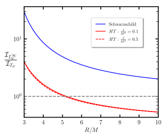
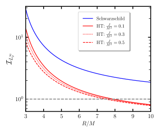
  Figure 3: In the left pane we show the comparison between two approaches of enhancement calculations using luminosity at infinite distance $(L^{\infty}_{\nu})$ and local temperature of neutrinosphere $(T_{\nu})$ as a function of $\frac{R}{M}$. In the right pane we show the comparison between Schwarzchild and HT metrics using the $\mathcal{I}_{\nu}^{\infty}$ as a function of $\frac{R}{M}$. In both cases, HT case has been presented for different $\frac{J}{M^{2}}$ values to study its dependency.

  Using the energy deposition rates for Schwarzchild and HT metrics, we define a quantity $\frac{\mathcal{I}_{L_{\nu}^{\infty}}}{\mathcal{I}_{T_{\nu}}}$ by taking the ratio of Eqs. 65 and 70. Doing that we find the comparison between the two approaches based on the luminosity at the observer $(L_{\nu}^{\infty})$ at an infinite distance and the local temperature of the neutrinosphere $(T_{\nu})$. According to the case involving Schwarzschild metric $\frac{\mathcal{I}_{L_{\nu}}^{\infty}}{\mathcal{I}_{T_{\nu}}}>1$, however, the case with HT metric gives $\frac{\mathcal{I}_{L_{\nu}}^{\infty}}{\mathcal{I}_{T_{\nu}}}<1$ for $\frac{R}{M}>5.21$ and the dependence on the dimensionless quantity $\frac{J}{M^{2}}$ is weak for case of HT metric. In addition to being different by a scaling factor, the method based on $L_{\nu}^{\infty}$ does not depend on the local physics of the GRB and therefore, we use this method in our analyses. Now in the right panel of Fig. 3 we further investigate the effect of Schwarzchild and HT metric using Eq. 65. We find that the quantity $\mathcal{I}_{L^{\infty}_{\nu}}$ decreases with $\frac{R}{M}$ irrespective of the metric. For HT metric, the dependence on $\frac{J}{M^{2}}$ becomes stronger for $\frac{R}{M}<8$ and for $\frac{R}{M}>8$, the quantity $\mathcal{I}_{L^{\infty}_{\nu}}<1$. The probability for neutrinos to interact reduces due to the effect of angular momentum, in addition there is also a rotational red-shift present as a result of non zero off diagonal element in the metric. The combined effect makes the quantity $\mathcal{I}_{L^{\infty}_{\nu}}$ in HT case lower than that of the Schwarzschild case irrespective of $R/M$.

• Modified gravity models: We consider two modified gravity models to compare the enhancements with the Schwarzchild and HT cases. For example, the modified gravity scenarios are (a) Born Infeld generalization of Reissner-Nordst$\ddot{o}$rm (BIRN) and (b) Charged Galileon (CG). We describe these moldes below:

  • Born Infeld generalization of Reissner-Nordst$\ddot{o}$rm: The BIRN solution describes the non-linear generalization of the Reiner-Nordst$\ddot{o}$rm solution characterized by mass $(M)$, charge $(Q)$ and Born-Infeld parameter $(b)$ of the object under consideration which are related to the magnitude of the magnetic field coupled to the gravty at $r=0$. As a result the BIRN solution reduces to the usual Reissner-Nordst$\ddot{o}$rm asymptotically. The corresponding action is given by

    $$S=\int d^{4}x\;\sqrt{-g}\left(\frac{1}{16\pi}\mathcal{R}+\mathcal{L}\right)$$ (77)

    where $\mathcal{R}$ is the Ricci scalar and $\mathcal{L}$ symbolizes the electromagnetic part of the action satisfying the invariants of the EM field [66]. The line element in this case is then given by

    $$ds^{2}=-f(r,Q,b)dt^{2}+f(r,Q,b)^{-1}dr^{2}+r^{2}d\Omega^{2}$$ (78)

    where

    $$f(r,Q,b)=1-\frac{2M}{r}+\frac{2}{3}b^{2}r^{2}\left(1-\sqrt{1+\frac{Q^{2}}{b^{2}r^{4}}}\right)+\frac{2Q^{2}}{3r}\sqrt{\frac{b}{Q}}F\left(\arccos{\frac{br^{2}/Q-1}{br^{2}/Q+1}},\frac{1}{\sqrt{2}}\right),$$

    $$F(\beta,k)=\int_{\beta}^{\infty}(1-k^{2}\sin^{2}s)^{-1/2}ds$$ (79)

    and $F(\beta,k)$ is the Legendre elliptic function. Since the trajectory function is quite lengthy for this metric, we do not provide it here. Hence the energy deposition rate can be calculated using the same methods as it is done in case of Schwarzschild metric as shown in previous section using Eq. 52.

  • Charged Galileon: The CG solutions correspond to a subclass of Horndeski theories [67]. There exists a non minimal coupling between the scalar and gravity. In this case the action takes the form

    $$S=\frac{1}{16\pi}\int d^{4}x\;\sqrt{-g}\left(R-\frac{1}{4}F_{\mu\mu}F^{\mu\nu}+\beta G^{\mu\nu}\nabla_{\mu}\phi\nabla_{\nu}\phi-\eta\partial_{\mu}\phi\partial^{\mu}\phi\right.-\left.\frac{\gamma}{2}\nabla^{\mu}\phi\nabla^{\nu}\phi\left(F_{\mu\sigma}F_{\nu}^{\sigma}-\frac{g_{\mu\nu}}{4}F^{\alpha\beta}F_{\alpha\beta}\right)\right)$$ (80)

    where $\phi$ is the gauge field and $G_{\mu\nu}\nabla_{\mu}\phi\nabla_{\nu}\phi$ represents the non minimal coupling between gravity and scalar field. The term proportional to $\gamma$ represents the coupling between stress tensor of gauge field with scalar field. Solving the field equation and imposing spherical symmetry, we can get the line element following [177] as

    $$ds^{2}=-fdt^{2}+f^{-1}dr^{2}+r^{2}d\Omega^{2},\;\;f=1-\frac{2M}{r}+\frac{\eta r^{2}}{3\beta}+\gamma\frac{(Q^{2}+P^{2})}{4\beta r^{2}}$$ (81)

    Since $\eta/3\beta=-\Lambda$, taking $\eta<0,\gamma,\beta>0$ and redefining $\gamma(Q^{2}+P^{2})/4\beta=M^{2}q$, the function $f(r)$ becomes

    $$f(r,M,\Lambda,q)=1-\frac{2M}{r}-\Lambda r^{2}+M^{2}\frac{q}{r^{2}}.$$ (82)

    Here $M$ is the mass of the object under consideration, $(Q,q)$ are related to the electric charge of the object under consideration and $\Lambda$ is the cosmological constant. In the following analysis, we consider $\Lambda=0$ since the metric is not flat asymptotically with a non-zero $\Lambda$ and thus we restrict ourselves to variation of the parameter $q$. The CG metric reduces to the Schwarzschild metric in the case of $\Lambda=0,q=0$. Hence the energy deposition rate can be calculated using the same methods as it is done in the case of Schwarzschild metric as shown in the previous section using Eq. 52.

To infer bounds on $M_{Z^{\prime}}/g_{X}$, we use the energy deposition rate calculated from various metrics and the following expression

$$\dot{Q}_{\rm{BSM}}^{GR}\leq\dot{Q}_{\rm{obs}}-\dot{Q}_{\rm{SM}}^{GR}$$ (83)

where the left-hand side denotes the BSM contribution from $Z^{\prime}$ and its interference with $W$ and $Z$ bosons while on the right-hand side, we have the observed energy deposition rate minus the SM contribution. GR stands for the metric under consideration. To estimate $\dot{Q}_{\rm obs}$, we use the brightest GRB event named GRB 221009A [59] whose isotropic energy was $E_{\gamma,iso}\simeq 1.2\times 10^{55}$ erg [178, 179, 180, 181, 179, 182, 183]. The true energy can be calculated using the relation given by $E_{true}=(1-\cos\theta_{j})E_{\gamma,iso}$ [184], where $\theta_{j}$ for GRB221009A is $1.5^{\degree}$ [59]. Using $\dot{Q}_{obs}=E_{true}/t$, we get the observed energy deposition rate to be $4\times 10^{51}erg/s$ where $t=1s$ is the time frame within which neutrinos deposit the energy [35]. In cases where $\dot{Q}_{SM}^{GR}$ is within 10% of $\dot{Q}_{obs}$, we estimate bounds by requiring $\dot{Q}_{BSM}^{GR}\leq\sigma$, where $\sigma$ is the observational uncertainty. We take $\sigma\simeq 0.1(0.01)\;\dot{Q}_{obs}$ for 10%(1%) uncertainty, respectively.

Using Eq. 83 we can calculate $\dot{Q}_{BSM/SM}^{GR}$ following the framework given in Eq. 72 for different cases of Schwarzchild, HT, BIRN and CG. We show the estimated bounds on the ratio of the energy deposition rates $(\dot{Q}_{BSM}^{GR}/\dot{Q}_{SM}^{GR})$ from Eq. 83 with respect to $M_{Z^{\prime}}/g_{X}$ represented by different horizontal colored straight lines in Fig. 4 for different metric and different $U(1)$ charges. We compute the same directly estimating the energy deposition rates for BSM and SM scenarios under a particular metric background being represented by different curved lines in Fig. 4 for different $U(1)$ charges. If the horizontal lines move downwards, the effect is dominated by the corresponding metric and moving upward shows enhancement by the BSM scenarios.

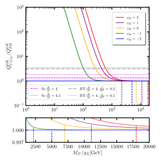
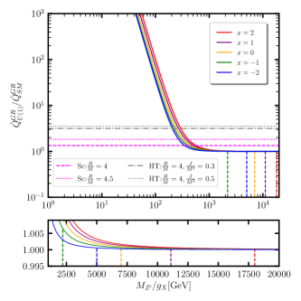
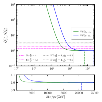
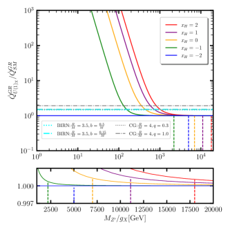
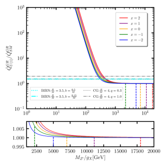
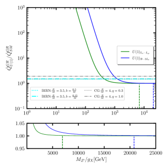
Figure 4: Enhancement in energy deposition rates for different $U(1)$ scenarios compared to SM for Schwarzchild, HT (upper panel) and BIRN and CG (lower panel) with respect to $M_{Z^{\prime}}/g_{X}$. The perpendicular lines show LEP-II bounds on $M_{Z^{\prime}}/g_{X}$.

	$\dot{Q}_{\rm{obs}}=4\times 10^{51}$ erg	$\dot{Q}_{\rm{obs}}=4\times 10^{51}$ erg	$\dot{Q}_{\rm{obs}}=4\times 10^{51}$ erg	$\dot{Q}_{\rm{obs}}=4\times 10^{51}$ erg
			(Modified Gravity)	(Modified Gravity)
	$M_{Z^{\prime}}/g_{X}$(GeV)	$M_{Z^{\prime}}/g_{X}$(GeV)	$M_{Z^{\prime}}/g_{X}$(GeV)	$M_{Z^{\prime}}/g_{X}$(GeV)
$U(1)_{X}$	$\frac{R}{M}^{\rm Sc}=3.67$	$\frac{R}{M}^{\rm Sc}=5$	$\frac{R}{M}^{\rm CG}=3.5$,$q=0.3$,$I=0.0$	$\frac{R}{M}^{\rm CG}=5$,$q=0.3$, $I=0.$
$x_{H}=2$	1999.16(6013.49)	726.455	2003.79(6028.71)	701.488
$x_{H}=1$	1430.2(4294.8)	522.041	1433.5(4305.66)	504.179
$x_{H}=0$	855.208(2552.6)	316.951	857.161(2559.05)	306.264
$x_{H}=-1$	257.075(633.401)	118.529	257.523(634.841)	115.18
	$\frac{R}{M}^{\rm HT}=3$,$\frac{J}{M^{2}}=0.37$	$\frac{R}{M}^{\rm HT}=5$,$\frac{J}{M^{2}}=0.37$	$\frac{R}{M}^{\rm BIRN}=3$, $\frac{b}{M}=0.5$	$\frac{R}{M}^{\rm BIRN}=5$, $\frac{b}{M}=0.5$
$x_{H}=2$	2006.79(6038.55)	489.047	2001.54(6021.3)	651.935
$x_{H}=1$	1435.64(4312.68)	351.975	1431.89(4300.37)	468.711
$x_{H}=0$	858.423(2563.21)	214.773	856.21(2555.91)	285.015
$x_{H}=-1$	257.813(635.772)	84.6959	257.305(634.14)	108.397
$U(1)_{q+xu}$	$\frac{R}{M}^{\rm Sc}=3.67$	$\frac{R}{M}^{\rm Sc}=5$	$\frac{R}{M}^{\rm CG}=3.5$, $q=0.3$, $I=0.0$	$\frac{R}{M}^{\rm CG}=5$,$q=0.3$, $I=0.0$
$x=2$	953.466(2863.2)	348.028	955.667(2870.44)	336.119
$x=1$	855.208(2552.6)	316.951	857.161(2559.05)	306.264
$x=0$	747.818(2200.3)	285.967	749.482(2205.83)	276.599
$x=-1$	631.473(1785.0)	257.742	632.789(1789.42)	249.753
$x=-2$	514.149(1266.8)	237.058	515.046(1269.68)	230.36
	$\frac{R}{M}^{\rm HT}=3$,$\frac{J}{M^{2}}=0.37$	$\frac{R}{M}^{\rm HT}=5$,$\frac{J}{M^{2}}=0.37$	$\frac{R}{M}^{\rm BIRN}=3$,$\frac{b}{M}=0.5$	$\frac{R}{M}^{\rm BIRN}=5$,$\frac{b}{M}=0.5$
$x=2$	957.09(2875.12)	234.65	954.596(2866.92)	312.474
$x=1$	858.423(2563.21)	214.773	856.21(2555.91)	285.015
$x=0$	750.559(2209.4)	195.638	748.672(2203.14)	257.921
$x=-1$	633.64(1792.27)	179.399	632.148(1787.27)	233.735
$x=-2$	515.625(1271.54)	169.392	514.61(1268.28)	216.795
$U(1)_{B-3L_{e}}$	$\frac{R}{M}^{\rm Sc}=3.67$	$\frac{R}{M}^{\rm Sc}=5$	$\frac{R}{M}^{\rm CG}=3.5$, $q=0.3$, $I=0.0$	$\frac{R}{M}^{\rm CG}=5$,$q=0.3$, $I=0.0$
	2556.20(7931.37)	828.27	2562.48 (7951.61)	795.86
	$\frac{R}{M}^{\rm HT}=3$,$\frac{J}{M^{2}}=0.37$	$\frac{R}{M}^{\rm HT}=5$, $\frac{J}{M^{2}}=0.37$	$\frac{R}{M}^{\rm BIRN}=3$, $\frac{b}{M}=0.5$	$\frac{R}{M}^{\rm BIRN}=5$,$\frac{b}{M}=0.5$
	2566.55(7964.7)	529.94	2559.42(7941.46)	732.16
$U(1)_{L_{e}-L_{\mu}}$	$\frac{R}{M}^{\rm Sc}=3.67$	$\frac{R}{M}^{\rm Sc}=5$	$\frac{R}{M}^{\rm CG}=3.5$, $q=0.3$, $I=0.0$	$\frac{R}{M}^{CG}=5$, $q=0.3$, $I=0.0$
	882.75(2700.2)	304.5	8884.86(2706.88)	293.41
	$\frac{R}{M}^{\rm HT}=3$, $\frac{J}{M^{2}}=0.37$	$\frac{R}{M}^{\rm HT}=5$,$\frac{J}{M^{2}}=0.37$	$\frac{R}{M}^{\rm BIRN}=3$, $\frac{b}{M}=0.5$	$\frac{R}{M}^{\rm BIRN}=5$, $\frac{b}{M}$=0.5
	886.23(2711.32)	200.92	883.83(2703.54)	271.58

Table 5: Bounds on $M_{Z^{\prime}}/g_{X}$ of different $U(1)$ scenarios depending on general $U(1)$ charges for Schwarzchild, HT, BIRN and CG cases respectively. Due to the leptonic charge assignments $L_{e}-L_{\tau}$ limits will be same as $L_{e}-L_{\mu}$.

The cross-over between the horizontal and curved lines shows bounds on $M_{Z^{\prime}}/g_{X}$ for different $U(1)$ models and metric parameters. Since the metric-dependant part cancels out in $\dot{Q}_{BSM}^{GR}/\dot{Q}_{SM}^{GR}$, these curved lines represent the ratio of total BSM cross-section and SM cross section and thus always reach 1 asymptotically in $M_{Z^{\prime}}/g_{X}$. The estimated bounds with $10\%$ uncertainty are shown in Tab. 5. Bounds on $M_{Z^{\prime}}/g_{X}$ become stronger with a lower $R/M$ ratio compared to a higher $R/M$ ratio. In addition to that, we give results with $1\%$ uncertainty for the lower $R/M$ ratio in Tab. 5 as prospective cases.

Note that in the case of $U(1)_{X}$ scenario we find that for $x_{H}=-2$ there is no coupling between left-handed lepton doublet and $Z^{\prime}$. Therefore we do not find any bound for $x_{H}=-2$ in $U(1)_{X}$. Therefore in this case we consider $x_{H}=-1$, $0$, $1$ and $2$ respectively where $x_{H}=0$ is the B$-$L case. However, in case of $U(1)_{q+xu}$ scenario we consider $x_{H}=-2$, $-1$, $0$, $1$ and $2$ respectively where $x_{H}=1$ is the B$-$L case. In $U(1)_{q+xu}$ scenario left-handed lepton doublet always couples with $Z^{\prime}$. In the case of the flavored scenarios we consider $B-3L_{e}$ case where electron neutrino is involved, similarly, we consider $L_{e}-L_{\mu}$ case because first and second-generation leptons are charged under the $U(1)$ gauge group. The same thing happens in the case of $L_{e}-L_{\tau}$ scenario where first and third-generation leptons are charged under the $U(1)$ gauge group. Therefore in the case of flavored scenarios, GRB contributes in those cases where $Z^{\prime}$ couples with electron. Corresponding bounds are shown in Tab. 5.

In Fig. 4 we show perpendicular lines which are the LEP-II bounds on $M_{Z^{\prime}}/g_{X}$ for different $U(1)$ charges depending on the models and these are obtained from Tab. 2 considering $M_{Z^{\prime}}>>\sqrt{s}$. As a result, LEP-II does not affect the bounds obtained from GRB directly. However, limits can be estimated on $M_{Z^{\prime}}/g_{X}$ from LEP-II which will constrain the $U(1)$ couplings for $M_{Z^{\prime}}>\sqrt{s}$. Therefore the perpendicular lines resemble indirect bounds on varying $\dot{Q}_{BSM}^{GR}/\dot{Q}_{SM}^{GR}$ for a fixed $M_{Z^{\prime}}/g_{X}$. In this analysis, we consider the large VEV scenario for different $U(1)$ scenarios, as a result, the quantity $M_{Z^{\prime}}/2g_{X}$ reduces to the VEV of the general $U(1)$ theory. Therefore we will further utilize only such $M_{Z^{\prime}}/g_{X}$ values from Tab. 5 which will satisfy this condition to estimate constraints on $g_{X}-M_{Z^{\prime}}$ plane for different $U(1)$ charges depending on the model.

IV Neutrino-DM scattering from cosmic blazars and AGN

To investigate neutrino-DM interaction in general $U(1)$ extension of SM, we extend models with potential DM candidates. In this paper, we separately consider three alternative types of DM candidates: (i) scalar, (ii) Dirac and (iii) Majorana. We explain these aspects for $U(1)_{X}$, $U(1)_{q+xu}$, $L_{i}-L_{j}$ and $B-3L_{i}$ scenarios in the following:

• Scalar DM: We introduce a potential complex scalar DM candidate in general $U(1)_{X}$ model where a complex scalar field $\Phi_{1}=\{1,1,0,Q_{\chi}\}$ can be introduced in the model with an odd $Z_{2}$ parity where remaining particles are even under $Z_{2}$ transformation . Due to this fact, $\Phi_{1}$ interacts with the other fields of the model through $Z^{\prime}$. This complex scalar field can interact with the scalar sector through the potential in the following way

  $$V\supset\lambda_{\rm minx_{1}}(H^{\dagger}H)(\Phi_{1}^{\ast}\Phi_{1})+\lambda_{\rm minx_{2}}(\Phi^{\dagger}\Phi)(\Phi_{1}^{\ast}\Phi_{1}).$$ (84)

  We assume $\lambda_{\rm mix_{1,2}}$ to be very small in the line of scalar mixing considered in Eq. 4 taken to be small. Like the $U(1)_{X}$ scenario, the complex scalar DM will act exactly in the same way in $U(1)_{qx+u}$, $U(1)_{B-3L_{i}}$ and $L_{i}-L_{j}$ scenarios. The interaction between complex scalar DM, $Z^{\prime}$ and neutrinos is described in the following way

  $$\mathcal{L}_{\rm DM}^{\rm scalar}=Q_{\chi}g_{X}Z^{\prime}_{\mu}\Big{\{}\Phi_{1}^{\ast}(\partial_{\mu}\Phi_{1})-(\partial_{\mu}\Phi_{1}^{\ast})\Phi_{1}\Big{\}}+m_{\rm{DM}}^{2}\Phi_{1}^{\ast}\Phi_{1}+g_{X}Q_{\ell}\overline{\nu_{L}}\gamma^{\mu}\nu_{L}Z^{\prime}_{\mu}.$$ (85)

  where $Q_{\chi}$ in the first term is the general $U(1)$ charge of the potential complex scalar DM candidate, the second term represents the mass of the complex scalar DM where $m_{\rm DM}$ is the DM mass and $Q_{\ell}$ is the general $U(1)$ charge of the neutrinos representing the third term following Eq. 9, respectively.

  

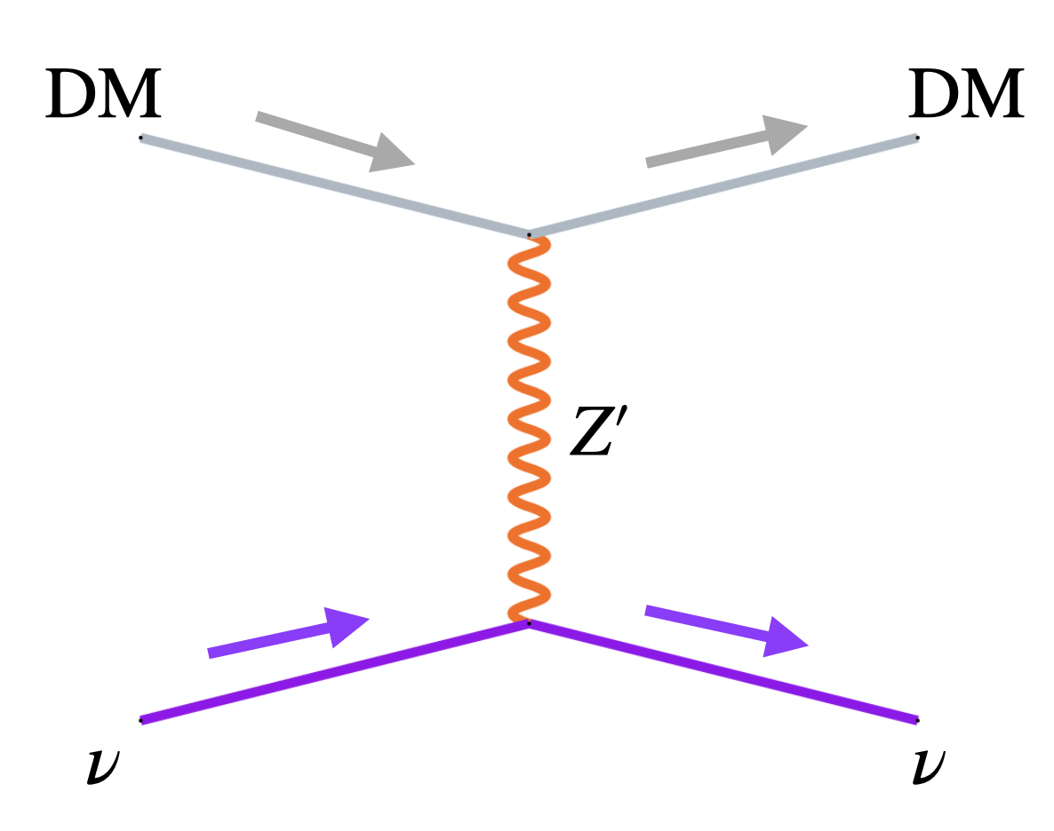
  Figure 5: Neutrino-DM scattering in $t-$channel mediated by $Z^{\prime}$ boson in laboratory frame and DM represents either of complex scalar, Majorana and Dirac type particle.

  Using these facts we estimate the differential scattering cross section for the $\nu-$DM scattering in $t-$channel mediated by $Z^{\prime}$ gauge boson in the laboratory frame as, see Fig. 5,

  $$\frac{d\sigma}{dE_{\nu}^{\prime}}=\frac{g_{X}^{4}Q_{\ell}^{2}Q_{\chi}^{2}}{8\pi}\frac{m_{\rm DM}}{E_{\nu}^{2}}\frac{(2E_{\nu}E_{\nu}^{\prime}-m_{\rm DM}(E_{\nu}-E_{\nu}^{\prime})}{\{M_{Z^{\prime}}^{2}+2\;m_{\rm DM}(E_{\nu}-E_{\nu}^{\prime})\}^{2}}$$ (86)

  where $Q_{\ell}$ depends on the general $U(1)$ scenario for a neutrino with incoming and outgoing energies $E_{\nu}$ and $E^{\prime}_{\nu}$ respectively.

  In case of $U(1)_{X}$ scenario, considering $x_{\Phi}=1$ we find that $Q_{\ell}=(-\frac{x_{H}}{2}-1)$. For $x_{H}=-2$, there is no interaction between $\nu_{L}$ and $Z^{\prime}$ which is $U(1)_{R}$ case. In this case we consider gauge kinetic mixing to be extremely small due to simplicity. Now, considering $x_{H}=-1$ we find $Q_{\ell}=-\frac{1}{2}$. In addition to that for $x_{H}=0$, $Q_{\ell}=-1$ which represents the B$-$L case. In $U(1)_{q+xu}$ scenario we find the DM charge as $-1$ and the charge of the neutrino is $-1$, too. These charges can be obtained from Tab. 1. The charges are the same for three generations of neutrinos.

  On the other hand, we consider flavored $Z^{\prime}$ cases where we have $L_{i}-L_{j}$ scenario, one of the neutrino charges is $+1$ and the other one is $-1$, where the third flavor is not charged under $U(1)_{L_{i}-L_{j}}$ gauge group. The detained particle content without DM candidate is given in Tab. 3. However, from Eq. 86 we find $\frac{d\sigma}{dE_{\nu}^{\prime}}$ is dependent on $Q_{\ell}^{2}$ therefore sign of $Q_{\ell}$ does not affect the analysis. There is another flavored $Z^{\prime}$ scenario which is known as $B-3L_{i}$ case. In this scenario $i$th generation neutrino has a charge of $-3$ under $U(1)_{B-3L_{i}}$ gauge group while the remaining two generations of the neutrinos are uncharged. We mention that complex scalar DM candidate in flavored scenario will follow Eqs. 85 and 86 respectively. The gauge coupling could be allowed validating the perturbative limit as $g_{X}|Q_{\chi}|<\sqrt{4\pi}$.

• Majorana DM: An interesting alternative of a potential DM candidate is Majorana fermion which can be introduced in the context of general $U(1)$ extension of the SM where we have three generations of RHNs. In this case, we simply use $Z_{2}$ parity for the content of the fields, where one generation of the RHNs is odd under $Z_{2}$ but the remaining fields in the model are $Z_{2}$ even ensuring the stability of the potential DM candidate. Following this framework we consider $N^{3}_{R}$ as a potential DM candidate while neutrino mass and flavor mixing are governed by the remaining two generations of the RHNs, $N^{1,2}_{R}$. Depending on the gauge structure DM interacts with the SM sector through $Z^{\prime}$ considering the contribution from scalar to be small due to the smallness of $\lambda^{\prime}$. Following the gauge structure, we write the interaction Lagrangian of the DM candidate and neutrinos from Eqs. 2 and 9 in the following way

  $$-\mathcal{L}_{\rm DM_{1}}^{\rm Majorana}=\{Y_{N}^{3}\Phi\overline{({N_{R}^{3}})^{c}}N^{3}_{R}+h.c.\}+g_{X}Q_{\chi}N^{3}\gamma^{\mu}\gamma_{5}P_{R}N^{3}Z_{\mu}^{\prime}+g_{X}Q_{\ell}\overline{\nu_{L}}\gamma^{\mu}\nu_{L}Z^{\prime}_{\mu}$$ (87)

  where the first term generates the DM mass after general $U(1)$ breaking, the second term represents the $Z^{\prime}-$DM interaction applying $x_{\Phi}=1$ and the third term represents the general $U(1)$ interaction between neutrino and $Z^{\prime}$. $Q_{\ell}$ is the general $U(1)$ charge of $\nu_{L}$. We estimate the $\nu-$DM differential scattering in $t-$ channel mediated by $Z^{\prime}$ gauge boson in laboratory frame, see Fig. 5,

  $$\frac{d\sigma}{dE_{\nu}^{\prime}}=\frac{g_{X}^{4}Q_{\ell}^{2}Q_{\chi}^{2}\;}{8\pi}\frac{m_{\rm DM}}{E_{\nu}^{2}}\frac{(E_{\nu}^{2}+{E^{\prime}_{\nu}}^{2}+m_{\rm DM}(E_{\nu}-E_{\nu}^{\prime}))}{\{M_{Z^{\prime}}^{2}+2\;m_{\rm DM}(E_{\nu}-E^{\prime}_{\nu})\}^{2}}$$ (88)

  where incoming and outgoing neutrino energies are $E_{\nu}$ and $E_{\nu}^{\prime}$, respectively. In the $U(1)_{X}$ scenario, $Q_{\chi}=x_{\Phi}=-1$ and $Q_{\ell}$ is the general $U(1)$ charge of neutrinos which can be obtained from Tab. 1. We find that $Q_{\ell}=(-\frac{x_{H}}{2}-1)$ which further reduces to $U(1)_{R}$ case for $x_{H}=-2$ having no interaction between $\nu_{L}$ and $Z^{\prime}$. For simplicity we consider gauge kinetic mixing to be extremely small. Taking $x_{H}=-1$ we find $Q_{\ell}=-\frac{1}{2}$, whereas for $x_{H}=0$ we obtain $Q_{\ell}=-1$ which is the B$-$L case. The neutrino charge in $U(1)_{q+xu}$ scenario is $-1$, and if we consider $x=1$, then DM charge in this context will be $Q_{\chi}=\frac{-4+x}{3}=-1$. These charges can be obtained from Tab. 1. The charges are the same for three generations of neutrinos.

  In this context we point out another interesting aspect which follows the same framework of the general $U(1)_{X}$ scenario as shown in Tab. 1, there are two Higgs doublets which are differently charged under $U(1)_{X}$ gauge group which protects the second Higgs doublet $(H_{2}=\{1,2,-\frac{1}{2},-\frac{x_{H}}{2}+3\})$ from any direct interaction with the SM fermions. After solving the gauge and mixed gauge-gravity anomalies we find that the $U(1)_{X}$ charge assignments of the three generations of RHNs follow a different pattern where first two generations have $(-4,-4)$ charge $(N_{R}^{1,2}=\{1,1,0,-4\})$ and the third generation has $5$ charge ${N_{R}^{3}=\{1,1,0,Q_{\chi}=5\}}$. The third generation RHN can be considered as a potential DM candidate and we do not need an additional $Z_{2}$ symmetry in this case. The $U(1)_{X}$ charge assignment of the SM fermions are exactly same as the $U(1)_{X}$ case mentioned in Tab. 1 with $x_{\Phi}=1$. In this model we introduce three SM singlet scalar fields $\Phi_{(A,B,C)}=\{1,1,0,(8,-10,-3)\}$. The corresponding interactions relevant to the DM sector is given below

  $$-\mathcal{L}_{\rm DM_{2}}^{\rm Majorana}=\{Y_{N}^{3}\Phi_{B}\overline{({N_{R}^{3}})^{c}}N^{3}_{R}+h.c.\}+5g_{X}N^{3}\gamma^{\mu}\gamma_{5}P_{R}N^{3}Z_{\mu}^{\prime}+g_{X}Q_{\ell}\overline{\nu_{L}}\gamma^{\mu}\nu_{L}Z^{\prime}_{\mu}$$ (89)

  where the first term generates the DM mass after general $U(1)$ breaking, the second term represents the $Z^{\prime}-$DM interaction, and the third term represents the general $U(1)$ interaction between $\nu$ and $Z^{\prime}$. Here $Q_{\ell}$ is the general $U(1)$ charge of $\nu_{L}$. In this scenario $N^{1,2}_{R}$ will participate in neutrino mass generation mechanism after the $U(1)_{X}$ symmetry breaking . We estimate the $\nu-$DM differential scattering in $t-$ channel mediated by $Z^{\prime}$ gauge boson in laboratory frame

  $$\frac{d\sigma}{dE_{\nu}^{\prime}}=25\frac{g_{X}^{4}Q_{\ell}^{2}\;}{8\pi}\frac{m_{\rm DM}}{E_{\nu}^{2}}\frac{(E_{\nu}^{2}+{E^{\prime}_{\nu}}^{2}+m_{\rm DM}(E_{\nu}-E_{\nu}^{\prime}))}{\{M_{Z^{\prime}}^{2}+2\;m_{\rm DM}(E_{\nu}-E^{\prime}_{\nu})\}^{2}}$$ (90)

  where incoming and outgoing neutrino energies are $E_{\nu}$ and $E_{\nu}^{\prime}$, respectively.

  In addition to the above aspects, we take flavored $Z^{\prime}$ scenarios in our account. One of them is $L_{i}-L_{j}$ case where $i$th generation neutrino has $U(1)$ charge $+1$ and $j$th generation neutrino has $U(1)$ charge $-1$. In this case, the third flavor is not charged under $U(1)_{L_{i}-L_{j}}$ gauge group. The field content of this scenario is given in Tab. 3 without a DM candidate. We consider $N^{1}_{R}$ as a potential Majorana DM candidate with odd $Z_{2}$ parity whereas other fields in the particle content have even $Z_{2}$ parity. In this case, while $N^{2,3}_{R}$ participate in the neutrino mass generation mechanism. Hence in this case $U(1)$ charge of the DM candidate will be $Q_{\chi}=1$. From Eq. 88 we find $\frac{d\sigma}{dE_{\nu}^{\prime}}$ is dependent on $Q_{\chi}^{2}Q_{\ell}^{2}$ therefore sign of $Q_{\chi,\ell}$ do not affect the analysis. We consider another flavored $Z^{\prime}$ scenario called $B-3L_{i}$. In this scenario, $i$th generation neutrino has a charge of $-3$ under the corresponding general $U(1)$ gauge group while the remaining two generations are not charged. Detailed particle contents without DM candidate are given in Tab. 4. We introduce an odd $Z_{2}$ parity for the $i$th generation RHN which has $-3$ charge under $U(1)_{B-3L_{i}}$ and the remaining two generations participate in neutrino mass generation and flavor mixing mechanisms. The negative or positive charge of the neutrino and DM candidate does not affect the analysis. Needless to mention that DM candidates in flavored case will also follow Eqs. 87 and 88 respectively.

• Dirac DM: We extend the general $U(1)$ field contents with $\chi_{L,R}=\{1,1,0,Q_{\chi}\}$ which will potentially be Dirac type DM candidate which could be applied to study $\nu-$DM scattering. We assign the general $U(1)$ charge for the DM candidate in such way that ensures the stability of the DM candidate. Under the $U(1)_{X}$ scenario we introduce SM-singlet and weakly interacting fermion $(\chi_{L,R})$ with $U(1)_{X}$ charge $n_{\chi}$ through which they interact with $Z^{\prime}$ as

  $$\mathcal{L}_{\rm DM}^{\rm Dirac}=i\overline{\chi_{L}}\gamma^{\mu}(\partial_{\mu}+ig_{X}Q_{\chi}Z^{\prime}_{\mu})\chi_{L}+i\overline{\chi_{R}}\gamma^{\mu}(\partial_{\mu}+ig_{X}Q_{\chi}Z^{\prime}_{\mu})\chi_{R}+(m_{\rm DM}\overline{\chi_{L}}\chi_{R}+h.c.)+g_{X}Q_{\ell}\overline{\nu_{L}}\gamma^{\mu}\nu_{L}Z^{\prime}_{\mu}$$ (91)

  with $\chi=\chi_{L}+\chi_{R}$ we obtain

  $$\mathcal{L}_{\rm DM}^{\rm Dirac}=i\overline{\chi}\gamma^{\mu}(\partial_{\mu}+ig_{X}Q_{\chi}Z^{\prime}_{\mu})\chi+m_{\rm DM}\overline{\chi}\chi$$ (92)

  and considering $x_{\Phi}=1$. To ensure the stability of the DM candidate, we prevent some charges for the DM candidate prohibiting some couplings. The restricted interactions and the corresponding forbidden charges are given in Tab. 6 to ensure stability of the DM candidate. Except these charges all the other possibilities could be allowed validating the perturbative limit as $g_{X}|Q_{\chi}|<\sqrt{4\pi}$.

  Models	Forbidden interaction	Forbidden charge assignments
  	terms	to stabilize scalar DM
  $U(1)_{X}$	$\overline{\chi_{R}^{c}}N_{R}+\overline{\chi_{L}}N_{R}+\overline{\ell_{L}}H\chi_{R}+\Phi\overline{\chi_{R}^{c}}N_{R}+\Phi^{\ast}\overline{\chi_{R}^{c}}N_{R}$	$Q_{\chi}\neq\{\pm 3x_{\Phi},\pm x_{\Phi}\}$ $=\{\pm 3,\pm 1\}$, taking $x_{\Phi}=1$
  	$+\Phi\overline{\chi_{L}}N_{R}++\Phi^{\ast}\overline{\chi_{L}}N_{R}$
  $U(1)_{q+xu}$	$\overline{\chi_{R}^{c}}N_{R}+\overline{\chi_{L}}N_{R}+\overline{\ell_{L}}H\chi_{R}+\Phi\overline{\chi_{R}^{c}}N_{R}+\Phi^{\ast}\overline{\chi_{R}^{c}}N_{R}$	$Q_{\chi}\neq\pm 3\Big{(}\frac{-4+x}{3}\Big{)},~{}\pm\Big{(}\frac{-4+x}{3}\Big{)},~{}\pm\Big{(}\frac{2+x}{3}\Big{)}$
  	$+\Phi\overline{\chi_{L}}N_{R}++\Phi^{\ast}\overline{\chi_{L}}N_{R}$
  $U(1)_{L_{i}-L_{j}}$	$\overline{\chi_{R}^{c}}N_{R}^{i}+\overline{\chi_{R}^{c}}N_{R}^{j}+\overline{{\chi_{R}}^{c}}N_{R}^{k}+\overline{\chi_{L}}N_{R}^{i}+\overline{{\chi_{L}}^{c}}N_{R}^{j}+\overline{{\chi_{L}}^{c}}N_{R}^{k}$
  	$\overline{\ell_{L}^{i}}H\chi_{R}+\overline{\ell_{L}^{j}}H\chi_{R}+\overline{\ell_{L}^{k}}H\chi_{R}+\Phi^{\ast}\overline{\chi_{R}^{c}}N_{R}^{i}+\Phi^{\ast}\overline{\chi_{R}^{c}}N_{R}^{j}+\Phi^{\ast}\overline{\chi_{R}^{c}}N_{R}^{k}$	$Q_{\chi}\neq\pm 3,~{}\pm 2,~{}\pm 1,~{}0$
  	$\Phi\overline{\chi_{R}^{c}}N_{R}^{i}+\Phi\overline{\chi_{R}^{c}}N_{R}^{j}+\Phi\overline{\chi_{R}^{c}}N_{R}^{k}+\Phi\overline{\chi_{L}}N_{R}^{i}+\Phi\overline{\chi_{L}}N_{R}^{j}+\Phi\overline{\chi_{L}}N_{R}^{k}+$
  	$\Phi^{\ast}\overline{\chi_{L}}N_{R}^{i}+\Phi^{\ast}\overline{\chi_{L}}N_{R}^{j}+\Phi^{\ast}\overline{\chi_{L}}N_{R}^{k}$
  	(with $i\neq j\neq k$)
  $U(1)_{B-3L_{i}}$	$\overline{\chi_{R}^{c}}N_{R}^{i}+\overline{\chi_{R}^{c}}N_{R}^{j,k}+\overline{\chi_{L}}N_{R}^{i}+\overline{{\chi_{L}}^{c}}N_{R}^{j,k}+\overline{\ell_{L}^{i}}H\chi_{R}+\overline{\ell_{L}^{j,k}}H\chi_{R}$
  	$+\Phi\overline{\chi_{R}^{c}}N_{R}^{i}+\Phi\overline{\chi_{R}^{c}}N_{R}^{j,k}+\Phi^{\ast}\overline{\chi_{R}^{c}}N_{R}^{i}+\Phi^{\ast}\overline{\chi_{R}}N_{R}^{j,k}$	$Q_{\chi}\neq\pm 9,~{}\pm 6,~{}\pm 3,~{}0$
  	$+\Phi\overline{\chi_{L}^{c}}N_{R}^{i}+\Phi\overline{\chi_{L}^{c}}N_{R}^{j,k}+\Phi^{\ast}\overline{\chi_{L}^{c}}N_{R}^{i}+\Phi^{\ast}\overline{\chi_{L}}N_{R}^{j,k}$
  	(with $i\neq j\neq k$)

  Table 6: Prohibited interactions and charges for the Dirac DM in the context of general $U(1)$ extensions.

  In this scenario we consider a UV complete theory which might allow the neutrino to mix with the DM candidate through non-renormalizable, higher dimensional operators for odd $n_{\chi}$ therefore we can safely choose $Q_{\chi}$ as either even numbers or fractional numbers. The $\nu-$DM scattering process depends on $x_{H}$ coming from $Q_{\ell}$, the $U(1)_{X}$ charge of the neutrino. For simplicity we consider the gauge kinetic mixing to be very small. We estimate the $\nu-$DM differential scattering in $t-$channel mediated by $Z^{\prime}$ gauge boson in laboratory frame as, see Fig. 5,

  $$\frac{d\sigma}{dE_{\nu}^{\prime}}=\frac{g_{X}^{4}Q_{\ell}^{2}Q_{\chi}^{2}\;}{8\pi}\frac{m_{\rm DM}}{E_{\nu}^{2}}\frac{(E_{\nu}^{2}+{E^{\prime}_{\nu}}^{2}-m_{\rm DM}(E_{\nu}-E_{\nu}^{\prime}))}{\{M_{Z^{\prime}}^{2}+2\;m_{\rm DM}(E_{\nu}-E^{\prime}_{\nu})\}^{2}}$$ (93)

  where $E_{\nu}$ and $E_{\nu}^{\prime}$ are the energies of the incoming and outgoing neutrinos. Here $m_{\rm DM}$ is the mass of Dirac type DM candidate. In case of $U(1)_{X}$ scenario considering $x_{\Phi}=1$, $Q_{\ell}=-\frac{x_{H}}{2}-1$ which manifests chiral scenario while in case of $U(1)_{q+xu}$ scenario $Q_{\ell}=-1$, respectively. Similarly, for the flavoured scenarios, the $U(1)$ charge of $\nu_{L}$ will depend on the gauge structure and corresponding generation given in Tabs. 3 and 4, respectively. Finally, the differential scattering cross section from Eq. 93 is proportional to $Q_{\ell}^{2}Q_{\chi}^{2}$, therefore the sign of the charge of either $\nu_{L}$ and DM candidate do not affect the analysis.

Neutrino-DM scattering can be also constrained from different cosmic observations from blazars and Active Galactic Nuclei (AGN) at the IceCube observatory in the south pole. AGN are supermassive black holes at the center of galaxies that are actively accreting matter. Blazars are a type of AGN that emit intense radiation across the electromagnetic spectrum, from radio waves to gamma rays. Due to their high luminosity and variability, blazars have been studied extensively in astrophysics, particularly in the context of understanding the properties of the relativistic jets that are thought to be responsible for their emission. Recently, there has been growing interest in using blazars as astrophysical probes of BSM physics from the aspects of astroparticle physics. In our paper, we specifically focus on using two AGN-associated events to study the interactions between neutrinos and dark matter, and to constrain the properties of the $Z^{\prime}$ boson, which arises in general $U(1)$ extensions of the SM. The two AGN that is of interest in this paper are:

• TXS 0506+056 [185]: The blazar TXS 0506+056, located at a distance of approximately 4 billion light years from Earth, was the first blazar observed to emit a high-energy neutrino. A 290 TeV neutrino event, known as IC- 170922A, was observed by the IceCube experiment in 2017 and was verified to be coming from the blazar TXS 0506+056. This has since spurred significant interest in using blazars as a tool for studying neutrino-dark matter interactions.

• NGC 1068 [82]: IceCube reported an excess of $79^{+22}_{-20}$ neutrinos identified with the active galaxy NGC 1068 at a significance of $4.2\sigma$. The NGC1068 galaxy is located at a distance of approximately 14 million light years from earth. According to the AGN classification based on their optical emission lines, NGC1068 is a Seyfert 2 galaxy characterized by their broad emission lines resulting from interaction the radiation and surrounding gas. NGC1068 is identified to be the first steady source of neutrino emission.

To study the effects of the $\nu$-DM scattering on the initial neutrino flux, we will solve the cascade equation defined as

$$\frac{d\Phi}{d\tau}=-\sigma\;\Phi+\int_{E^{\prime}}^{\infty}dE\;\frac{d\sigma}{dE^{\prime}}\Phi(E)$$ (94)

where $E$ is the initial energy of the neutrino, $E^{\prime}$ is the final energy of the neutrino, $\tau=\Sigma(r)/m_{\rm DM}$ is the accumulated column density of the DM along the line of sight. Defining a dimensionless quantity, $x=\tau\frac{m_{DM}}{\Sigma(r)}$, the equation can be rewritten as

$$\frac{d\Phi}{dx}=-\sigma\frac{\Sigma(r)}{m_{\rm DM}}\;\Phi+\frac{\Sigma(r)}{m_{\rm DM}}\int_{E^{\prime}}^{\infty}dE\;\frac{d\sigma}{dE^{\prime}}\Phi(E)$$ (95)

where $x\in[0,1]$. Here $\sigma$ and $\Phi$ are the total cross section and flux, respectively. Then the cascade equation given in the form of Eq. 95 can be solved using the vectorization method as described in [116]. In our analysis we fix the DM mass for simplicity as a free parameter. This further helps us to estimate the constraints on the parameters of different general $U(1)$ scenarios. In the following subsection, we will describe the analysis for both the blazar TXS 0506+056 and NGC 1068 in detail.

IV.1 TXS 0506 + 056

Our study of TXS 0506+056 highlights the potential of blazars to constrain the properties of $Z^{\prime}$ boson arising from $U(1)$ extensions of the standard model. The neutrino flux emitted by the blazar can be evaluated using the lepto-hadronic model. In the lepto-hadronic model, the jets of blazars are thought to be composed of a plasma of relativistic electrons and protons in which the electrons are accelerated to very high energies which then emit synchrotron radiation. The expected neutrino flux is then given by [186, 80]

$$\log_{10}\frac{\Phi_{\nu}}{\text{cm}^{2}}=-\mathcal{F}_{0}x-\frac{\mathcal{F}_{1}x}{1+\mathcal{F}_{2}|x|^{\mathcal{F}_{3}}}$$ (96)

where $\mathcal{F}_{0}=13.22$, $\mathcal{F}_{1}=1.498$, $\mathcal{F}_{2}=-0.00167$, $\mathcal{F}_{3}=4.119$, and $x=\log_{10}(E_{\nu}/\text{TeV})$ with $E_{\nu}\in[10^{-1.2},10^{4.2}]$ TeV being the energy of the neutrinos.

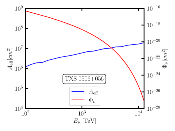
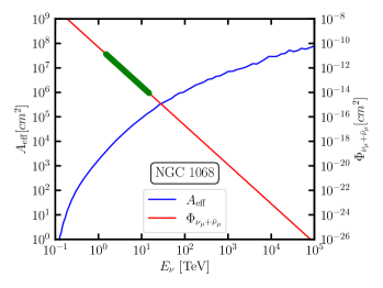
Figure 6: The flux predicted by the lepto-hadronic model and the effective area of detection obtained from IceCube data. The left panel shows an effective area for the blazar event TX0506 + 056 while the right panel shows the same quantities for NGC 1068. The region marked in green for NGC 1068 where IceCube reliably measures the flux. The energy range corresponding to the green region is $E_{\nu}~{}\in[1.5,15]$ TeV which has been considered in this paper.

Then, the number of events observed at IceCube can be calculated using

$$N_{\rm events}=t_{\rm obs}\int dE\;A_{\rm eff}(E)\;\Phi_{\nu}(E_{\nu})$$ (97)

where $A_{\text{eff}}$ is the effective area of detection of high energy neutrinos and it describes the probability for a neutrino to convert into a muon inside the detector which is obtained from the IceCube data [187]. In this analysis, we take $t_{\rm obs}=898$ days for the IC86a campaign which lasted from Julian day 57161 - 58057. The total flux and effective area of detection of high energy neutrinos from the blazars are plotted in the left panel of Fig. 6 using Eq. 96 and the IceCube data repository.

In this analysis, we consider a model in which potential DM candidates surround a central black hole (BH), so that the neutrinos from the blazar will interact with DM candidates. Therefore we need to assign a quantity called column density which resembles the measure of the DM concentration being an intervening substance between neutrinos and observer. This makes it possible to constrain $\nu$-DM scattering by studying the blazar. We define the dark matter column density following [69]. The accumulated DM column density is given by

$$\tau=\frac{\Sigma(r)}{m_{\rm DM}}=\int dr\frac{\rho_{\rm DM}}{m_{\rm DM}}$$ (98)

where $\rho_{\rm DM}$ is the spike density profile of DM and is given by $\rho_{\rm DM}(r)=\frac{\rho^{\rm core}\tilde{\rho}(r)}{\rho^{\rm core}+\tilde{\rho}(r)}$. Here $\rho^{\rm core}$ is the maximum core density set by the DM annihilation in the inner spike region and is given by the relation $\rho^{\rm core}\simeq\frac{m_{\rm DM}}{\langle\sigma v\rangle_{\rm eff}\;t_{\rm BH}}$ where $t_{\rm BH}\simeq 10^{9}$ years is the age of the BH following ‘Bachal-Wolf’ solution from [188], $\langle\sigma v\rangle_{\rm eff}$ is the effective thermal averaged DM annihilation cross section.

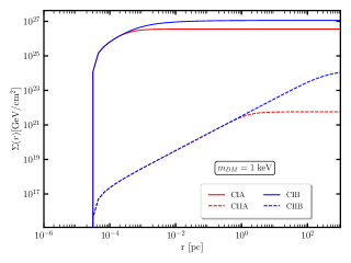
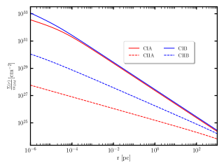
Figure 7: Accumulated column density with respect to distance $r$ from the BH, for a fixed DM mass $m_{\rm DM}=10^{-3}$ MeV and for different benchmark scenarios, is shown in the left panel, while accumulated column density per unit DM mass with respect to DM mass is shown in the right panel.

The density profile $\tilde{\rho}(r)$ is defined as $\tilde{\rho}(r)=\mathcal{N}\Big{(}1-4\frac{R_{\rm Sc}}{r}\Big{)}^{3}r^{-\alpha_{\rm sp}}$ where $R_{\rm Sc}=2GM_{\rm BH}$ is the Schwarzschild radius of the BH and $\alpha_{\rm sp}$ is the slope of the DM spike profile. Here $\mathcal{N}$ is a renormalization constant. It can be determined by requiring that the mass of the spike be of the same order as $M_{\rm BH}$ [189]. Hence we write

$$\mathcal{N}=\frac{M_{\rm BH}}{4\pi\int_{4R_{\rm Sc}}^{10^{5}R_{\rm Sc}}r^{2-\alpha_{\rm sp}}\Big{(}1-4\frac{R_{\rm Sc}}{r}\Big{)}^{3}dr}.$$ (99)

DM particles within $4R_{\rm Sc}$ are captured by the BH[190]. It has been estimated in [191] that the BH mass of the blazar TXS 0506+056 as $3.09\times 10^{8}M_{\odot}$. Additionally, we consider that the canonical thermally averaged generic WIMP type DM annihilation cross section has an upper limit of $\langle\sigma v\rangle\simeq 3\times 10^{-26}$ cm³ s^-1 [4]. Following this aspect, we take in our analysis the benchmark of the effective thermally averaged DM annihilation cross sections as $\langle\sigma v\rangle_{\rm eff}=10^{-34}$ cm³ s^-1 and $3\times 10^{-26}$ cm³ s^-1. Following [192, 193, 194, 195, 196] we summarize that, applying the assumptions of collisionless and phase space density conserving particle dark matter scenario, dissipationless galaxy simulations predict a power law cusp in DM density $\rho_{\rm DM}\propto r^{-\gamma}$ with $1<\gamma<1.5$ or even for $\gamma<1$ [197] where $\gamma$ is the slope of the initial profile. However, in the vicinity of a galactic center the mass in the inner core is dominated by the supermassive black hole which may undergo an adiabatic growth in the central region of the BH due to an effect of a small speed accereting luminous and nonluminous objects [198, 199, 200, 201, 202], the DM cusp may enhance spiking up the form $\rho_{\rm{DM}}\propto r^{-\alpha_{\rm sp}}$ where $2.3<\alpha_{\rm sp}=(9-2\gamma)/(4-\gamma)<2.5$ [69]. It has been shown in [189] that enhancement becomes weaker due to the instantaneous appearance of the BH being induced by mergers of progenitor halos resulting a slope in spike and identified as $\alpha_{\rm sp}=1.33$. On the other hand simulation studies showed that mergers of BHs in the progenitor halos may reduce the density of the DM to a reduced power law $\rho_{\rm DM}\propto r^{-1/2}$ due to kinetic heating of the particles during merger [203, 204, 205] and it further grows away from the central region of the DM distribution [206]. According to the previous studies [207, 208, 209, 210, 211] we identify $\gamma$ as the power spectrum index parametrizing the inner cusp of initial DM halo density. Another aspect pointed out in [196] is that the galactic center may have a compact cluster of stars in addition to the supermassive BH. These stars may scatter DM particles causing an evolution to the DM distribution function leading to a quasi-equilibrium profile through two-body relaxation for the stars and DM. Demanding a steady state scenario, the DM distribution function can be obtained as a power-law of energy and the DM density can be obtained as a power-law of radius providing unique solutions being independent of the initial conditions [188, 212, 213]. Considering the DM mass to be negligibly smaller than the stellar mass, the quasi-equilibrium solution further reduces to $\alpha_{\rm sp}=3/2$ for two-component system of DM and starts described by a collisional Fokker-Planck equation [214] with no energy flux. In our further analysis, we consider two benchmark cases $\alpha_{\rm sp}=3/2$ and $7/3$, and the complete benchmark cases are written in Tab. 7.

Benchmark scenarios	Effective DM annihilation	Spike slope $(\alpha_{\rm sp})$
	cross sections $(\langle\sigma v\rangle_{\rm eff}~{}\rm{in}~{}\rm{cm}^{3}\rm{s}^{-1})$
CIA	$10^{-34}$
		$\alpha=7/3$
CIIA	$3\times 10^{-26}$
CIB	$10^{-34}$
		$\alpha=3/2$
CIIB	$3\times 10^{-26}$

Table 7: Different benchmark scenarios for TXS 0506 + 056 and NGC 1068 considered in this article.

Using these benchmark scenarios, following Eq. 98 and applying $\rho_{\rm DM}$ for blazars we show the accumulated DM column density with respect to $r$ in the left panel of Fig. 7. In this case, the behaviour of the accumulated DM column density changes with $\alpha_{\rm sp}$ depending on $r$. For fixed $\langle\sigma v\rangle_{\rm eff}$, $\Sigma(r)$ changes for $\alpha_{\rm sp}$. The lower slope gives a denser profile after $r>1$ pc. For fixed $\alpha_{\rm sp}$ we find that lower $\langle\sigma v\rangle_{\rm eff}$ gives a denser profile due to its presence in the denominator of $\rho^{\rm core}$. The density profile per unit DM mass is shown in the right panel of Fig. 7 depending on DM mass for the several cases given in Tab. 7. For fixed $\alpha_{\rm sp}$, the quantity $\Sigma(r)/m_{\rm DM}$ becomes different for $m_{\rm DM}<10^{-3}$ GeV will be useful to solve the cascade equation for the blazars.

IV.2 NGC 1068

The functional form of the neutrino flux can be written as

$$\Phi_{\nu_{\mu}+\bar{\nu}_{\mu}}(E_{\nu})=\Phi_{\rm ref}\Big{(}\frac{E_{\nu}}{E_{\rm ref}}\Big{)}^{-a}.$$ (100)

From [215] we find that Eq. 100 reduces to $4.9032\times 10^{-11}E_{\nu}^{-3.196}$, where $E_{\nu}\in[0.1,10^{4}]$ TeV considering $E_{\rm ref}=1$ TeV and the central value of the observed events 79 at IceCube. Using $\Phi_{\nu_{\mu}+\bar{\nu}_{\mu}}(E_{\nu})$ and corresponding $A_{\rm eff}$ in Eq. 97 with $t_{\rm obs}=3186$ days [82], we calculate the number of expected events in the form of muon neutrinos. The number of events reduces to 31 within the IceCube considered range $E_{\nu}\in[1.5,15]$ TeV. The flux $\Phi_{\nu_{\mu}+\bar{\nu}_{\mu}}$ and $A_{\rm eff}$ for the event NGC1068 can be directly obtained from the IceCube data [215] and the correspondence has been shown in the right panel of Fig. 6. Here the green region corresponds to reliable measurement of the flux taking muon neutrinos detected by the IceCube detectors. Due to the effect of neutrino oscillation over an astrophysical distance, the flux for all three flavors will be enhanced by a factor of three [216, 217]. The $\nu-$DM scattering has a possibility to dissipate the energy of the neutrino from the source towards an observer on Earth. It has been pointed out in [80] that $\nu-$DM scattering could shift the flux peak of a spectrum to lower energies resulting in a larger amount of the expected number of neutrinos at the detectable energy range of IceCube. As a result, bounds on $\nu-$DM scattering cross-section may have stronger bounds considering a flux having a peak at higher energy compared to the observed ones. Therefore we can use the flux given in Eq. 100 as the initial flux to estimate conservative bounds on $\nu-$DM scattering cross-section.

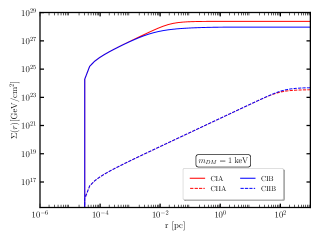
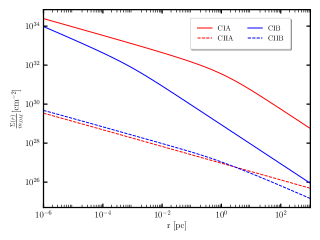
Figure 8: Accumulated column density with respect to distance $r$ from the BH, for a fixed DM mass $m_{\rm DM}=10^{-3}$ MeV and for different benchmark scenarios, is shown in the left panel, while accumulated column density per unit DM mass with respect to DM mass is shown in the right panel.

To study the $\nu-$DM scattering, there exists an important parameter called the DM density profile. From [69], we come to know if the accretion of the BH is adiabatic and we neglect the relativistic effects so that DM density profile can be expressed in the form $\rho_{\rm DM}\simeq\rho_{\rm sc}(\frac{r}{r_{\rm sc}})^{-\gamma}$, that is as a cusp in the region close to the BH with $\rho_{\rm sc}$ and $r_{\rm sc}$ being the scale density and scale radius, respectively. Then the DM density profile evolves into $\tilde{\rho}_{\rm DM}(r)\simeq\rho_{R}\Big{(}1-4\frac{R_{\rm Sc}}{r}\Big{)}^{3}\Big{(}\frac{R_{s}}{r}\Big{)}^{\alpha_{\rm sp}}$, where $R_{s}$ is a typical size of the spike profile according to [69, 218]. Due to the presence of a dense medium in the inner region of a galaxy, DM may experience scattering which may vary the $\alpha_{\rm sp}$. As a result, we consider two slops, $3/2$ and $7/3$, in this analysis. This modification is possible within a radius of influence $(r_{I})$ inside a supermassive BH [219, 196, 220, 70]. The radius of influence defines a region where the gravitational effect of the supermassive BH affects the movement of the neighbouring stars; the radius of influence is generally less than the typical size of the spike profile. Now we define the DM spike density profile for $\alpha_{\rm sp}=3/2$ as

$$\rho_{3/2}=\begin{cases}\rho_{N}\left(1-4\frac{R_{\rm Sc}}{r}\right)^{3}\left(\frac{r_{I}}{r}\right)^{3/2},&r_{i}\leq r\leq r_{I}\\ \rho^{\prime}_{N}\left(\frac{R_{s}}{r}\right)^{7/3},&r\geq r_{I}~{}(\rm outer~{}profile)\end{cases}$$ (101)

and that with $\alpha_{\rm sp}=7/3$ as

$$\rho_{7/3}=\;\rho_{N}\left(1-4\frac{R_{\rm Sc}}{r}\right)^{3}\left(\frac{R_{s}}{r}\right)^{7/3},\;r\geq r_{i}$$ (102)

respectively. Here the inner radius of the spike is given by $r_{i}=4R_{\rm Sc}$ and $r_{I}=\frac{GM_{\rm BH}}{\sigma_{v}^{2}}\simeq 0.65$ kpc for a supermassive BH taking $\sigma_{v}$ as stellar velocity dispersion. The mass of the supermassive BH has been considered as $M_{\rm BH}=10^{7}M_{\odot}$ being consistent with the estimation of the DM halo mass $\mathcal{O}(10^{11}M_{\odot})$ NGC 1068 [221, 222]. For $\alpha_{\rm sp}=3/2$ we define the normalization density parameter as $\rho_{N}=\mathcal{N}r_{I}^{-3/2}$ and that for $\alpha_{\rm sp}=7/3$ we define $\rho_{N}=\mathcal{N}R_{s}^{-7/3}$ respectively. The function $\mathcal{N}$ can be defined as

$$\mathcal{N}=\frac{M_{\rm BH}}{4\pi(f(\alpha_{\rm sp},r_{I})-f(\alpha_{\rm sp},r_{i}))},$$ (103)

considering

$$f(\alpha_{\rm sp},r)=r^{-\alpha_{\rm sp}}\left(\frac{r^{3}}{3-\alpha_{\rm sp}}+\frac{12R_{\rm Sc}r^{2}}{\alpha_{\rm sp}-2}-\frac{48R_{\rm Sc}^{2}r}{\alpha_{\rm sp}-1}+\frac{64R_{\rm Sc}^{3}}{\alpha_{\rm sp}}\right)$$ (104)

while $M_{\rm BH}\simeq 4\pi\int_{r_{i}}^{r_{I}}\rho_{\rm DM}(r)~{}r^{2}~{}dr$ [189, 190]. Here $\rho_{\rm DM}$ is given by

$$\rho_{\rm DM}=\begin{cases}0,&r\leq r_{i}\\ \frac{\rho_{\alpha_{\rm sp}}(r)\rho^{\rm core}}{\rho_{\alpha_{\rm sp}}(r)+\rho^{\rm core}},&r_{i}\leq r\leq R_{s}\\ \frac{\rho_{\rm NFW}(r)\rho^{\rm core}}{\rho_{\rm NFW}(r)+\rho^{core}},&r\geq R_{s}\end{cases}$$ (105)

where $\rho^{\rm core}\simeq\frac{m_{\rm DM}}{\langle\sigma v\rangle_{\rm eff}t_{\rm BH}}$. For the NFW halo profile, we define $\rho_{\rm NFW}(r)=\rho_{s}\left(\frac{r_{\rm sc}}{r}\right)\left(1+\frac{r}{r_{\rm sc}}\right)^{-2}$, where $\rho_{\rm sc}=0.35$ $\rm GeV/{cm}^{3}$, the scale parameter for the density profile is taken as $r_{\rm sc}=13$ kpc [103, 223], having consistency with the data of the supermassive BH in galaxy Milky Way [224] and having mass alike one in NGC 1068. In this context we mention that normalization density parameter $\rho_{N}^{\prime}\simeq\rho_{N}(r_{I}/R_{s})^{7/3}=\mathcal{N}r_{I}^{5/6}R_{s}^{-7/3}$ requiring that at $r=r_{I}$ then $\rho_{N}^{\prime}\to\rho_{3/2}^{\prime}$. Matching the conditions of spike and outer part of the halo as $\rho_{N}^{\prime},\rho_{N}\simeq\rho_{\rm sc}(R_{s}/r_{\rm sc})^{-\gamma}$ for $\alpha=3/2$ and $7/3$ where $R_{\rm Sc}<<r_{I}<R_{s}<<r_{\rm sc}$, we obtain

$$R_{s}=\begin{cases}\left(\frac{\mathcal{N}}{\rho_{\rm sc}r_{\rm sc}}\right)^{3/4}r_{I}^{5/8},&\alpha=3/2\\ \left(\frac{\mathcal{N}}{\rho_{\rm sc}r_{\rm sc}}\right)^{3/4},&\alpha=7/3\end{cases}$$ (106)

For NGC 1068 we consider $R_{\rm s}\simeq 0.7$ kpc which is greater than $r_{I}$ under the parameters used throughout this paper. Finally we define the accumulated column density of DM as

$$\Sigma(r)=\int_{R_{\rm EM}}^{r}dx\;\rho_{\rm DM}(x)$$ (107)

where $R_{\rm EM}$ ($\approx 30R_{\rm Sc}=2.8\times 10^{-5}$ pc) is the position at which neutrinos are expected to be produced with respect to the BH. The DM density $\rho_{\rm DM}$ is given by the expression in Eq. 105 and integrating over the radius for different benchmark cases from Tab. 7 we show the column density in the left panel of Fig. 8 starting from $r>R_{\rm EM}$. The accumulated column density for different DM models saturate to a constant value around $r\simeq 10$ pc and $100$ pc depending on $\alpha_{\rm sp}$ and $\langle\sigma v\rangle_{\rm eff}$. Hence we come to a conclusion that at the Earth, where $r\simeq 14.4$ Mpc, the accumulated column density is considered to be a constant. On the other hand we show the accumulated column density per unit DM mass for different cases given in Tab. 7 which will have implications to solve the cascade equation for AGN.

V Results and discussions

We study different scattering and beam-dump experiments for different $U(1)$ extensions of the SM to estimate bounds on $g_{X}-M_{Z^{\prime}}$ plane. Taking into account different cosmic bursts like GRB involving $\nu\bar{\nu}\to e^{+}e^{-}$ scattering, blazars and AGN involving $\nu-$DM scattering we estimate bounds on the $g_{X}-M_{Z^{\prime}}$ plane for different $U(1)$ extensions of the SM. Finally we compare our results.

V.1 Limit from LEP experiment

We estimate bounds on $\{M_{Z^{\prime}},g_{X}\}$ from the results of LEP-II measuring $e^{+}e^{-}\to\bar{f}f$ scattering cross section at the $Z$ peak with $f$ being the SM fermions [225]. The scattering cross sections are calculated including $Z^{\prime}$ exchanging diagram and it is compared with the observed value. We find that the strongest constraint can be obtained from the cross-section of $e^{+}e^{-}\to q\bar{q}$ process giving a hadronic final state whose value is $\sigma=45.44\pm 0.037$ nb. Then we obtain the upper limit of $g_{X}$ as a function of $M_{Z^{\prime}}$ requiring the estimated cross section is within the 90% C.L. of the observed one. Limits are given in Fig: 9-12 for the $U(1)_{X}$ and $U(1)_{q+xu}$ in the upper and lower panels. In case of $U(1)_{q+xu}$ scenario, these limits are shown by gray shaded area. We find similar limits for the $L_{e}-L_{\mu,\tau}$ scenarios in the upper and lower limits of Fig. 13 and those for $B-3L_{e}$ scenario are given in Fig. 15.

V.2 Limit from dark photon search at LHC experiments

Also we estimate bounds on $\{M_{Z^{\prime}},g_{X}\}$ from the results of CMS [148] and LHCb [145] experiments that search for dark photon $A^{\prime}$ decaying into $\mu^{+}\mu^{-}$ pair. These experiments provide us with the constraints on dark photon mass $m_{A^{\prime}}$ and kinetic mixing parameter $\epsilon$. We estimate the upper limit of our gauge coupling $g_{X}$ as a function of $M_{Z^{\prime}}$ in use of the following rescaling

$$g_{X}^{\rm max}(M_{Z^{\prime}}=m_{A^{\prime}})=\epsilon^{\rm max}(m_{A^{\prime}})e\sqrt{\frac{\sigma(pp\to A^{\prime})BR(A^{\prime}\to\mu^{+}\mu^{-})}{\sigma(pp\to Z^{\prime})BR(Z^{\prime}\to\mu^{+}\mu^{-})}},$$ (108)

where $\sigma(pp\to A^{\prime}(Z^{\prime}))$ is dark photon$(Z^{\prime})$ production cross section and $\epsilon^{\rm max}(m_{A^{\prime}})$ is the experimental upper limit of kinetic mixing parameter as a function of dark photon mass. We estimated the $A^{\prime}(Z^{\prime})$ production cross sections using CalcHEP3.5 implementing relevant interactions. Limits are given in Fig: 9-12 for the $U(1)_{X}$ and $U(1)_{q+xu}$ in the upper and lower panels. We find similar limits for the $B-3L_{\mu}$ scenario which are given in the upper panel of Fig. 16.

V.3 Limit from BaBar experiment

At the BaBar experiment, $e^{+}e^{-}$ collision produces dark photon via the process $e^{+}e^{-}\to A^{\prime}\gamma$. They search for visible $A^{\prime}$ decaying into $\{e^{+}e^{-},\mu^{+}\mu^{-},\text{light mesons}\}$ final states and invisible $A^{\prime}$ decaying into invisible final sate such as neutrinos. We rescale the upper limit of gauge coupling in the $U(1)_{B-L}$ case given in [146, 147] as a function of $Z^{\prime}$ mass to obtain that of $g_{X}$ in our model. For $Z^{\prime}$ decaying into visible modes, the rescaling formula is

$$g_{X}^{\rm max}(M_{Z^{\prime}})=g_{B-L}^{\rm max}(M_{Z^{\prime}})\sqrt{\frac{\sigma(e^{+}e^{-}\to\gamma Z^{\prime}_{B-L})BR(Z^{\prime}_{B-L}\to\text{visible states})}{\sigma(e^{+}e^{-}\to\gamma Z^{\prime})BR(Z^{\prime}\to\text{visible states})}},$$ (109)

where $Z^{\prime}_{B-L}$ indicate $Z^{\prime}$ boson in $U(1)_{B-L}$ case. For $Z^{\prime}$ decaying into invisible modes, the rescaling formula is

$$g_{X}^{\rm max}(M_{Z^{\prime}})=g_{B-L}^{\rm max}(M_{Z^{\prime}})\sqrt{\frac{\sigma(e^{+}e^{-}\to\gamma Z^{\prime}_{B-L})BR(Z^{\prime}_{B-L}\to\bar{\nu}\nu)}{\sigma(e^{+}e^{-}\to\gamma Z^{\prime})BR(Z^{\prime}\to\bar{\nu}\nu)}},$$ (110)

where all neutrino modes are summed up. Corresponding bounds are shown in Figs. 9-12 for $U(1)_{X}$ and $U(1)_{q+xu}$ scenarios and in Fig. 15 for $B-3L_{e}$ scenario, respectively. In case of $U(1)_{q+xu}$ scenario these bounds belong to the gray shaded region. Bounds for $L_{e}-L_{\mu,\tau}$ scenarios are shown in the upper and lower panels of Fig. 13.

V.4 Limits from dilepton searches from CMS and ATLAS

Studying dilepton production at $\sqrt{s}=13$ TeV proton-proton collider, we compare the production cross section $(\sigma^{\rm{model}})$ of dilepton mode (electron and muon) in our model having a trial value of $U(1)$ coupling $g^{\rm{model}}$ with the dilepton production cross section $(\sigma^{\rm{CMS/ATLAS}})$ given by the CMS[226] and ATLAS[165] collaborations at the LHC using sequential standard model(SSM) [227]. We used the CMS and ATLAS data with $\frac{\Gamma}{M_{Z^{\prime}}}=3\%$ where $\Gamma$ stands for the total decay width of $Z^{\prime}$. The CMS(ATLAS) collaboration produced the result with $140(139)$ fb^-1 luminosity. Hence we estimate bounds on $U(1)_{X}$ and $U(1)_{q+xu}$ scenarios following

$$g_{X}=g^{\rm{model}}\sqrt{\frac{\sigma^{\rm{CMS/ATLAS}}}{\sigma^{\rm{model}}}}$$ (111)

The model cross sections were estimated using the narrow width approximation as

$$\sigma^{\rm model}=\frac{8\pi^{2}}{3}~{}\sum_{q,\bar{q}}\int dx\int dy~{}q(x,Q),\bar{q}(x,Q)\times\frac{\Gamma(Z^{\prime}\to q\bar{q})}{M_{Z^{\prime}}}\delta(\hat{s}-M_{Z^{\prime}})\times\rm{BR}(Z^{\prime}\to 2\ell)$$ (112)

where $q(x,Q)$ and $\bar{q}(x,Q)$ are the parton distribution functions of the quark and antiquark respectively and $\hat{s}=xys$ is the invariant mass squared of the colliding quark at $\sqrt{s}$, the center of mass energy. We set the factorization scale at $Q=M_{Z^{\prime}}$ in the parton distribution function CTEQ6L[228]. These bounds are shown by CMS2$\ell$ and ATLAS2$\ell$ in Figs. 9-12. We find that around $150$ GeV $\leq M_{Z^{\prime}}\leq 6$ TeV CMS and ATLAS limits are almost comparable. In this mass range so-far LHC produces strongest upper limits depending on $M_{Z^{\prime}}$. We scale the corresponding results from CMS(ATLAS) to a projected 3 ab^-1 luminosity using

$$g_{X}^{\rm projected}\simeq g_{X}^{\rm{current}}\sqrt{\frac{139(140)~{}\rm fb^{-1}}{\mathcal{L}_{\rm projected}}}$$ (113)

shown by CMS$2\ell$-3 and ATLAS$2\ell$-3 respectively in the same figures. Using the same strategy we estimate bounds at current and projected luminosities of the LHC using only the two electron [226, 165], two muon [226, 165] and two tau [229, 230] final state from the CMS and ATLAS. Then we show bounds for the $B-3L_{e}$ scenario in Fig. 15 and for $B-3L_{\mu}$ and $B-3L_{\tau}$ scenarios in upper and lower panels of Fig. 16, respectively. In case of $B-3L_{\tau}$ we used the CMS(ATLAS) result at $2.2(36)$ fb^-1 luminosity.

V.5 Limits from LEP-II and prospective bounds from ILC

We have estimated limits on $M_{Z^{\prime}}/g_{X}$ for different chiral (for different charges) and flavored scenarios from LEP-II and prospective ILC at $\sqrt{s}=250$ GeV, 500 GeV and 1 TeV, respectively in Sec. II. Solving them for a range of $M_{Z^{\prime}}$ considering $M_{Z^{\prime}}>>\sqrt{s}$, we find different diagonal lines which are shown in Figs. 9-12 for different charges of the $U(1)_{X}$ (upper panel) and $U(1)_{q+xu}$ (lower panel) scenarios. Similar results have been derived for $L_{e}-L_{\mu}$ and $L_{e}-L_{\tau}$ scenarios and shown in Fig. 13. Due to electronic charge assignment, these bounds are same. Under the $B-3L_{e}$ scenario the first generation of lepton doublets is charged under the $U(1)$ gauge group, the corresponding constrains are shown in Fig. 15. In case of $U(1)_{X}$, $U(1)_{q+xu}$ and $B-3L_{e}$ scenarios we find that bounds obtained from LEP-II bounds are comparatively week compared to the LHC bounds, however, prospective bounds obtained from ILC at $\sqrt{s}=$ 250 GeV, 500 GeV and 1 TeV (ILC250, ILC500 and ILC1000) could provide stronger bounds than LHC. However, In case of $L_{e}-L_{\mu}$ and $L_{e}-L_{\tau}$ scenarios LEP-II provides strong bound for heavy $Z^{\prime}$ and prospective bounds from ILC could be stronger than LEP-II bounds. In future, such constrains could be improved involving initial and final state radiations, vector boson fusion process considering neutral and charged current interactions at electron-positron and muon colliders.

V.6 Constraints from proton/electron beam dump experiments

Here we summarize our estimation of constraints from beam dump experiments. For proton beam dump experiments LSND, PS191, NOMAD and CHARM, we estimate bound curves in our models by rescaling those of U(1)_B-L case [231]. Approximately, the curves for the upper bound on $\{m_{Z^{\prime}},g_{X}\}$ plane are derived applying the scaling [232, 17]

$$\tau_{Z^{\prime}}(g_{B-L}^{\rm max})\sim\tau_{Z^{\prime}}(g_{X}^{\rm max},x_{H},x_{\Phi})~{},$$ (114)

where $g_{B-L}$ indicates the gauge coupling in the U(1)_B-L model, and $\tau_{Z^{\prime}}$ is the lifetime of the $Z^{\prime}$. The curves for the lower bound are also scaled by using a formula

$$g_{X}^{\rm low}\sim g_{B-L}^{\rm low}\sqrt{\frac{{\rm BR}(M\to Z^{\prime}_{B-L}\gamma)~{}{\rm BR}(Z^{\prime}_{B-L}\to e^{+}e^{-})\tilde{\tau}_{Z^{\prime}}}{{\rm BR}(M\to Z^{\prime}\gamma)~{}{\rm BR}(Z^{\prime}\to e^{+}e^{-})\tilde{\tau}_{Z^{\prime}_{B-L}}}}~{},$$ (115)

where $\tilde{\tau}$ is lifetime with gauge coupling taken to be unity, and $Z^{\prime}$ is produced through meson decay processes with $M=\pi^{0}$ for LSND, PS191 and NOMAD, and $M=\eta$ for CHARM. In our estimation, meson decay branching ratio is obtained using the method given in Ref. [232].

For proton beam dump experiment $\nu$-cal, the $Z^{\prime}$ is dominantly produced via bremsstrahlung process. Here we adopt the results in ref. [19] for the constraint on $\{M_{Z^{\prime}},g_{X}\}$ where chiral structure of the $Z^{\prime}$ interactions is taken into account in estimating the $Z^{\prime}$ production cross section.

For electron beam dump experiments NA64, E774, Orsay and KEK, the bound curves are derived by rescaling the bounds of U(1)_B-L case as we did for the proton beam dump case. We approximately estimate the constraint for the upper region on $\{M_{Z^{\prime}},g_{X}\}$ plane by rescaling in use of Eq. 114, which is the same as the proton beam dump case. The constraint for the lower region is calculated by [17]

$$g_{X}^{\rm low}\sim g_{B-L}^{\rm low}\sqrt{\frac{2{\rm BR}(Z^{\prime}_{B-L}\to e^{+}e^{-})\tilde{\tau}_{Z^{\prime}}}{(x_{\ell}^{2}+x_{e}^{2}){\rm BR}(Z^{\prime}\to e^{+}e^{-})\tilde{\tau}_{Z^{\prime}_{B-L}}}}~{},$$ (116)

where $Z^{\prime}$ is considered to be produced through the bremsstrahlung process.

For electron beam dump experiments E137 and E141, we adopt the results in ref. [19] for the constraint on $\{M_{Z^{\prime}},g_{X}\}$ where chiral structure of the $Z^{\prime}$ interactions is taken into account in estimating the $Z^{\prime}$ production cross section. Following this line we estimate prospective bounds for DUNE-beam dump (DUNE-BD), FASER and FASER2 for $U(1)_{q+xu}$ case utilizing the B$-$L scenario given in [19]. The same methodology was followed to estimate constraints for the electron beam-dump scenario in ILC-beam dump (ILC-BD). These limits are give in Fig: 9-12 for the $U(1)_{X}$ and $U(1)_{q+xu}$ in the upper and lower panels. For $U(1)_{q+xu}$ scenario we show only the prospective DUNE-BD, FASER, FASER2 and ILC-BD bounds. Remaining bounds belong to the gray shaded region. We find similar limits for the $B-3L_{e}$ scenario which are given in Fig. 15 whereas for $B-3L_{\mu}$ and $B-3L_{\tau}$ the limits belong to the gray shaded area. The electron/positron beam-dump scanerions except for the above cases will appear in the $L_{i}-L_{j}$ scenarios where $L_{e}-L_{\mu,\tau}$ scenarios are shown in the upper and lower panels of Fig. 13.

V.7 Constraints from electron-(anti)neutrino scattering in neutrino experiments

We can also obtain constraints on $\{M_{Z^{\prime}},g_{X}\}$ from electron-(anti)neutrino scattering processes that are tested by neutrino experiments such as BOREXINO and TEXONO. The electron-(anti)neutrino scattering cross sections under the existence of $Z^{\prime}$ interactions are estimated to obtain the constraints on $Z^{\prime}$ mass and coupling. The differential cross section can be written as

$$\frac{d\sigma(\nu e)}{dT}=\left.\frac{d\sigma(\nu e)}{dT}\right|_{\rm SM}+\left.\frac{d\sigma(\nu e)}{dT}\right|_{Z^{\prime}}+\left.\frac{d\sigma(\nu e)}{dT}\right|_{\rm Int}$$ (117)

where $T$ is the electron recoil energy and the first, second and third terms in the RHS denote the contributions from the pure SM interactions, the pure $Z^{\prime}$ interactions and interference between the SM and $Z^{\prime}$ interactions. The terms in RHS are written by [17]. The purely SM contribution is

$$\left.\frac{d\sigma(\nu e)}{dT}\right|_{\rm SM} =\frac{2G_{F}^{2}m_{e}}{\pi E_{\nu}^{2}}\left(a^{2}_{1}E^{2}_{\nu}+a_{2}^{2}(E_{\nu}-T)^{2}-a_{1}a_{2}m_{e}T\right),$$ (118)

where $E_{\nu}$ is the initial neutrino energy. Here the coefficients $a_{1}$ and $a_{2}$ are written as

$$a_{1} = \left\{\sin^{2}\theta_{W}+\frac{1}{2},\ \sin^{2}\theta_{W},\ \sin^{2}\theta_{W}-\frac{1}{2},\ \sin^{2}\theta_{W}\right\}\ {\rm for}\ \{\nu_{e}e,\bar{\nu}_{e}e,\nu_{\beta}e,\bar{\nu}_{\beta}e\},$$

$$a_{2} = \left\{\sin^{2}\theta_{W},\ \sin^{2}\theta_{W}+\frac{1}{2},\ \sin^{2}\theta_{W},\ \sin^{2}\theta_{W}-\frac{1}{2}\right\}\ {\rm for}\ \{\nu_{e}e,\bar{\nu}_{e}e,\nu_{\beta}e,\bar{\nu}_{\beta}e\},$$ (119)

where $\beta=\{\mu,\tau\}$. The contribution from $Z^{\prime}$ exchanging diagram can be derived as

$$\left.\frac{d\sigma(\overset{(-)}{\nu}_{\alpha}e)}{dT}\right|_{Z^{\prime}} =\frac{g_{X}^{4}(x_{\ell})^{2}m_{e}}{4\pi E_{\nu}^{2}(2m_{e}T+M^{2}_{Z^{\prime}})}[(2E^{2}_{\nu}-2E_{\nu}T+T^{2})(b^{2}_{1}+b^{2}_{2})\pm 2b_{1}b_{2}(2E_{\nu}-T)T-m_{e}T(b^{2}_{1}-b_{2}^{2})],$$ (120)

where $b_{1}=\frac{x_{\ell}+x_{e}}{2}$ and $b_{2}=\frac{x_{\ell}-x_{e}}{2}$ with $x_{\ell,e}$, and the negative sign of $\pm$ is for anti neutrino processes. The contribution from interference between the SM and $Z^{\prime}$ are also obtained, depending on the processes, such that

$$\left.\frac{d\sigma(\nu_{e}e)}{dT}\right|_{\rm int} = \frac{G_{F}g_{X}^{2}x_{\ell}m_{e}}{\sqrt{2}\pi E^{2}_{\nu}(2m_{e}T+M^{2}_{Z^{\prime}})}[2E_{\nu}^{2}(b_{1}+b_{2})+(2E^{2}_{\nu}-2E_{\nu}T+T^{2})(b_{1}c_{1}+b_{2}c_{2})]$$

$$+T(2E_{\nu}-T)(b_{1}c_{2}+b_{2}c_{1})-m_{e}T(b_{1}-b_{2}+b_{1}c_{1}-b_{2}c_{2})],$$

$$\left.\frac{d\sigma(\bar{\nu}_{e}e)}{dT}\right|_{\rm int} = \frac{G_{F}g_{X}^{2}x_{\ell}m_{e}}{\sqrt{2}\pi E^{2}_{\nu}(2m_{e}T+M^{2}_{Z^{\prime}})}[2(E_{\nu}-T)^{2}(b_{1}+b_{2})+(2E^{2}_{\nu}-2E_{\nu}T+T^{2})(b_{1}c_{1}+b_{2}c_{2})]$$

$$-T(2E_{\nu}-T)(b_{1}c_{2}+b_{2}c_{1})-m_{e}T(b_{1}-b_{2}+b_{1}c_{1}-b_{2}c_{2})],$$

$$\left.\frac{d\sigma(\overset{(-)}{\nu}_{\beta}e)}{dT}\right|_{\rm int} = \frac{G_{F}g_{X}^{2}x_{\ell}m_{e}}{\sqrt{2}\pi E^{2}_{\nu}(2m_{e}T+M^{2}_{Z^{\prime}})}[(2E_{\nu}^{2}-2E_{\nu}T-T^{2})2(b_{1}c_{1}+b_{2}c_{1})\pm T(2E_{\nu}-T)(b_{1}c_{2}+b_{2}c_{1})]$$ (121)

$$-m_{e}T(b_{1}c_{1}-b_{2}c_{2})],$$

where $c_{1}=-1/2+2\sin^{2}\theta_{W}$ and $c_{2}=-1/2$. Then we calculate the differential cross sections and estimate the upper limit on $\{M_{Z^{\prime}},g_{X}\}$ for each experiment in the following way:

BOREXINO: The $\nu_{e}$-$e$ scattering is measured by the experiment with $\langle E_{\nu}\rangle=862$ keV and $T\simeq[270,665]$ keV for ${}^{7}B_{e}$ solar neutrino. To obtain the constraint on $\{m_{Z^{\prime}},g_{X}\}$, we require the total cross section should not be more than $8\%$ above that of the SM prediction [233].

TEXONO: The experiment measures $\bar{\nu}_{e}$-$e$ scatterings using 187 kg of CsI(Tl) scintillating crystal array with 29882/7369 kg-day of reactor ON/OFF data with electron recoil energy of $T\simeq[3,8]$ MeV. We estimate the $\chi^{2}$ value as

$$\chi^{2}=\sum_{\rm bin}\frac{(R_{\rm data}-R_{\rm th})^{2}}{\Delta R^{2}},$$ (122)

where $R_{\rm data}$ and $R_{\rm th}$ are the event ratios observed by the experiment and predicted by the cross-section from Eq. 117, $\Delta R$ is the experimental uncertainty, for each recoil energy bin taken from data in ref. [117], and anti-neutrino flux in the same reference is applied. The upper limit curve on $\{M_{Z^{\prime}},g_{X}\}$ plane is then obtained for $90\%$ C.L from the $\chi^{2}$ fit.

GEMMA: The experiment measures $\bar{\nu}_{e}$-$e$ scattering with 1.5 kg HPGe detector where energy of neutrino is $\langle E_{\nu}\rangle\sim 1$-$2$ MeV and flux is $2.7\times 10^{13}$ cm^-2s^-1. We estimated the $\chi^{2}$ value using the formula Eq. 122 for the data from ref. [234] with 13000 ON-hours and 3000 OFF-hours. Then we obtain the upper curve on $\{M_{Z^{\prime}},g_{X}\}$ with $90\%$ C.L.

CHARM-II: The experiment measures $\nu_{\mu}(\bar{\nu}_{\mu})$-electron scattering where $2677\pm 82$ and $2752\pm 88$ events are obtained for $\nu_{\mu}$ and $\bar{\nu}_{\mu}$ cases. The mean neutrino energy is $\langle E_{\nu_{\mu}}\rangle=23.7$ GeV and $\langle E_{\bar{\nu}_{\mu}}\rangle=19.1$ GeV, and the range of measured recoil energy is 3-24 GeV. We estimated the $\chi^{2}$ value using the formula Eq. 122 for the data from ref. [120, 121], and obtain the upper curve on $\{M_{Z^{\prime}},g_{X}\}$ with $90\%$ C.L.

These limits are given in Fig: 9-12 for the $U(1)_{X}$ and $U(1)_{q+xu}$ in the upper and lower panels. In case of $U(1)_{q+xu}$ scenario these bounds belong to the gray shaded region. Bounds for $L_{e}-L_{\mu,\tau}$ scenarios are shown in the upper and lower panels of Fig. 13 whereas for $L_{\mu}-L_{\tau}$ scenario these limits belong to the gray shaded region. We find similar limits for the $B-3L_{e}$ scenario which are given in Fig. 15 whereas for $B-3L_{\mu}$ and $B-3L_{\tau}$ the limits belong to the gray shaded area.

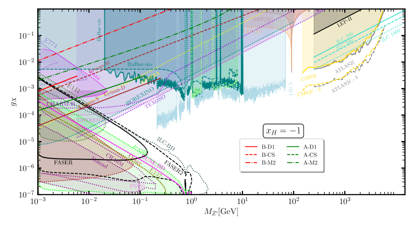
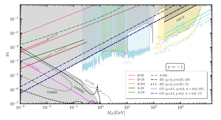
Figure 9: Limits on $g_{X}-M_{Z^{\prime}}$ plane for the $U(1)_{X}$ (upper panel) and $U(1)_{q+xu}$ (lower) scenarios considering $x_{H}=-1$ and $x=-1$, respectively.

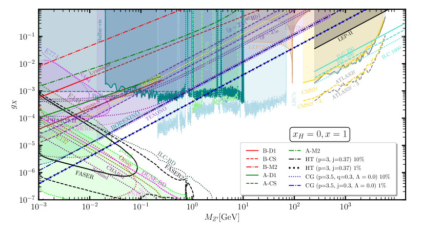
Figure 10: Limits on $g_{X}-M_{Z^{\prime}}$ plane for B$-$L scenario for $U(1)_{X}$ with $x_{H}=0$ and $U(1)_{q+xu}$ with $x=1$ respectively.

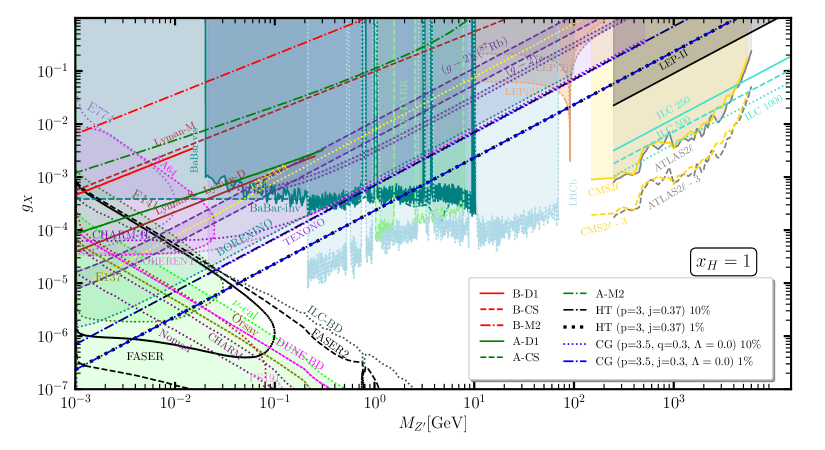
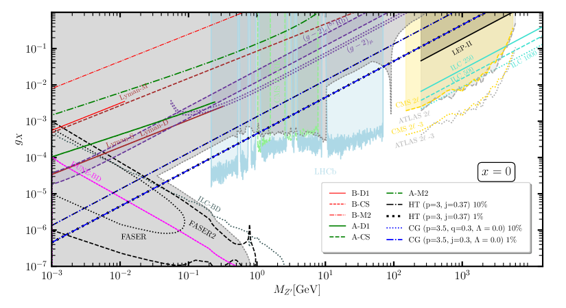
Figure 11: Limits on $g_{X}-M_{Z^{\prime}}$ plane for the $U(1)_{X}$ (upper panel) and $U(1)_{q+xu}$ (lower) scenarios considering $x_{H}=1$ and $x=0$, respectively.

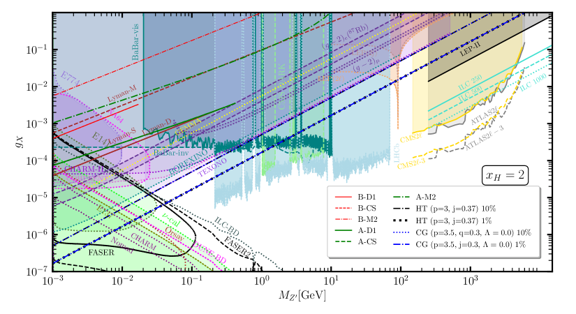
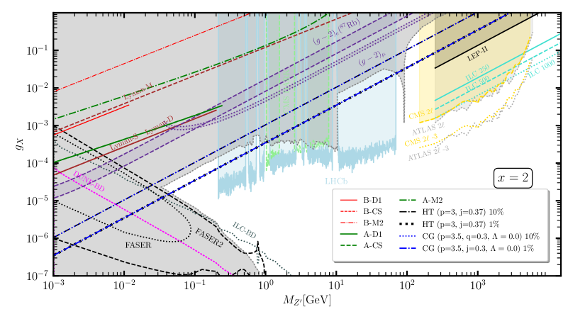
Figure 12: Limits on $g_{X}-M_{Z^{\prime}}$ plane for the $U(1)_{X}$ (upper panel) and $U(1)_{q+xu}$ (lower) scenarios considering $x_{H}=2$ and $x=2$, respectively.

V.8 Constraints from coherent neutrino-nucleus scattering

We also consider constraint on $\{M_{Z^{\prime}},g_{X}\}$ from coherent elastic neutrino-nucleus scattering (CE$\nu$NS) measured by COHERENT experiment with CsI and Ar targets [235]. In this work, we rescale the constraint on $U(1)_{B-L}$ case in Ref. [236, 237] by comparing number of events in $U(1)_{B-L}$ and other cases. The number of events at COHERENT experiment is estimated, adopting formulas in the reference, as follows. The differential cross section for CE$\nu$NS process is given by [238, 239]

$$\frac{d\sigma_{\nu-N}}{dT}(E,T)=\frac{G_{F}^{2}M}{\pi}\left(1-\frac{MT}{2E^{2}}\right)Q_{{\rm SM}+Z^{\prime}}^{2},$$ (123)

where $T$ is the recoil energy, $E$ is the neutrino energy, $M$ is the mass of target nucleus and $Q_{{\rm SM}+Z^{\prime}}$ is the factor coming from SM+$Z^{\prime}$ interactions. In the models $Q_{{\rm SM}+Z^{\prime}}$ is written such that

$$Q_{{\rm SM}+Z^{\prime}}=\left(g^{p}_{V}(\nu_{\ell})+2\epsilon^{uV}_{\ell\ell}+\epsilon^{dV}_{\ell\ell}\right)ZF_{Z}(|{\bf q}^{2}|)+\left(g^{n}_{V}(\nu_{\ell})+\epsilon^{uV}_{\ell\ell}+2\epsilon^{dV}_{\ell\ell}\right)NF_{N}(|{\bf q}^{2}|),$$ (124)

where $Z(N)$ is the number of proton(neutron) in the target nucleus, $g^{p(n)}_{V}$ is the neutrino-proton(neutron) coupling in the SM and $F_{Z(N)}(|{\bf q}^{2}|)$ is the from factors of the proton(neutron) for the target nucleus. The effective coupling $\epsilon^{qV}_{\ell\ell}$ is explicitly given by

$$\epsilon^{qV}_{\ell\ell}=\frac{g_{X}^{2}x_{\ell}x_{q}}{\sqrt{2}G_{F}({\bf q}^{2}+m^{2}_{Z^{\prime}})}.$$ (125)

For the neutrino-proton(neutron) coupling, we adopt the values of $g_{V}^{p}(\nu_{e})=0.0401$, $g_{V}^{p}=0.0318$ and $g_{V}^{n}=-0.5094$ for the SM [240, 241]. For the form factors $F_{Z(N)}(|{\bf q}^{2}|)$, we apply Helm parametrization [242] using proton rms radii $\{R_{p}({\rm Cs}),R_{p}({\rm I}),R_{p}({\rm Ar})\}=\{4.804,4.749,3.448\}$ [fm] and neutron rms radii $\{R_{n}({\rm Cs}),R_{n}({\rm I}),R_{n}({\rm Ar})\}=\{5.01,4.94,3.55\}$ [fm] [243, 244, 245].

For the CE$\nu$NS event rate in the COHERENT experiment, we use the neutrino fluxes that depend on the neutrino fluxes produced from the Spallation Neutron Source (SNS) at the Oak Ridge National Laboratories. They are written as

$$\frac{dN_{\nu_{\mu}}}{dE} = \eta\delta\left(E-\frac{m_{\pi}^{2}-m_{\mu}^{2}}{2m_{\pi}}\right),$$

$$\frac{dN_{\nu_{\bar{\mu}}}}{dE} = \eta\frac{64E^{2}}{m_{\mu}^{3}}\left(\frac{3}{4}-\frac{E}{m_{\mu}}\right),$$

$$\frac{dN_{\nu_{e}}}{dE} = \eta\frac{192E^{2}}{m^{3}_{\mu}}\left(\frac{1}{2}-\frac{E}{m_{\mu}}\right),$$ (126)

where $\eta=rN_{\rm POT}/(4\pi L^{2})$ with $r$, $N_{\rm POT}$ and $L$ being respectively the number of neutrinos per flavor that are produced for each proton-on-target (POT), the number of POT, and the distance between the source and the detector. For these values, we adopt $r=9\times 10^{-2}$, $N_{\rm POT}=13.7\times 10^{22}$ and $L=27.5$ m for Ar detector, and $r=0.08$, $N_{\rm POT}=17.6\times 10^{22}$ and $L=19.5$ m for CsI detector. The theoretical number of events for each energy bin in the COHERENT experiment is estimated by

$$N_{i}=N(\mathcal{N})\int^{T_{i+1}}_{T_{i}}dTA(T)\int_{E_{\rm min}}^{E_{\rm max}}dE\sum_{\nu=\nu_{e},\nu_{\mu},\nu_{\bar{\mu}}}\frac{dN_{\nu}}{dE}\frac{d\sigma_{\nu-N}}{dT}(E,T),$$ (127)

where $i$ distinguishes recoil energy bin, $E_{\rm min(max)}=\sqrt{MT/2}(m_{\mu}/2)$ and $A(T)$ is the energy-dependent reconstruction efficiency. We estimate the upper bound of coupling $g_{X}$ for each mass in our models by rescaling that of $U(1)_{B-L}$ case in ref. [237] where we compare the number of events for the upper bound on $U(1)_{B-L}$ and compare it with the number of events in each model to find the upper bound on $g_{X}$. Limits obtained from the coherent scenarios are shown in the upper panels of Fig. 9-12 for $U(1)_{X}$ case. These limits for the $U(1)_{q+xu}$ are not separately shown as they belong to the gray shaded region. Similar bounds for $B-3L_{e}$ are shown in Fig. 15.

V.9 $g-2$ of muon and electron

In the context of the general $U(1)_{X}$ extension of the SM, the left and right-handed fermions have different charges under the general $U(1)_{X}$ gauge group. These charges are family universal. However, in the case of flavoured scenarios the general $U(1)$ charge could depend on the generation of the fermions. Hence we write the general interaction Lagrangian as

$$\mathcal{L}_{\rm int}=g_{X}\overline{f}(q_{L}^{f}P_{L}+q_{R}^{f}P_{R})\gamma_{\mu}fZ^{\mu}$$ (128)

which can be reduced to leptonic interactions with $Z^{\prime}$. The vector and axial-vector couplings in general $U(1)_{X}$ extension can contribute to the magnetic moment of the muon and electron involving $Z^{\prime}$ in the loop satisfying $(g-2)_{\mu}$ results from [246]. Hence we can estimate bounds on the $g_{X}-M_{Z^{\prime}}$ plane for different charges in general $U(1)_{X}$ scenarios and flavored $U(1)$ scenarios. From [247, 248, 249] we write down the magnetic moment of muon (electron) using one loop $Z^{\prime}$ mediated processes as

$$\Delta{a_{\ell}}=\frac{g_{X}^{2}}{32\pi^{2}}\int_{0}^{1}dy\frac{\Big{\{}2y(1-y)(y-4)-4y^{3}\frac{m_{\ell}^{2}}{M_{Z^{\prime}}^{2}}\Big{\}}x_{a}^{2}+2(1-y)y^{2}x_{b}^{2}}{(1-y)(1-y\frac{m_{\ell}^{2}}{M_{{Z^{\prime}}^{2}}})+y\frac{m_{\ell}^{2}}{M_{Z^{\prime}}^{2}}}$$ (129)

where $m_{\ell}=m_{\mu(e)}$, $x_{a}=-\frac{3}{2}x_{H}-2x_{\Phi}$ and $x_{b}=-\frac{1}{2}x_{H}$ for the general $U(1)_{X}$ scenario. In the case of the $U(1)_{q+xu}$ scenario, we have $x_{a}=-\frac{5+x}{3}$ and $x_{b}=-\frac{x-1}{3}$ respectively. Similarly, we can calculate these coefficients for the flavored cases using the corresponding charges of the left and right-handed charged leptons. The current experimental ranges of muon $(g-2)$ is given by [250]

$$\Delta a_{\mu}=(24.9\pm 4.98)\times 10^{-10},$$ (130)

where the deviation from the world average of SM prediction is 5.0 $\sigma$ level. In addition to that, the current experimental ranges of electron $(g-2)$ are

$$\Delta a_{e}(^{133}\text{Cs})=-(8.8\pm 3.6)\times 10^{-13}~{}~{}\text{\cite[cite]{[\@@bibref{Number}{Parker:2018vye}{}{}]}},\,\,\,\,\,\Delta a_{e}(^{87}\text{Rb})=(4.8\pm 3.0)\times 10^{-13}~{}~{}\text{\cite[cite]{[\@@bibref{Number}{Morel:2020dww}{}{}]}}\,,$$ (131)

where the deviations from the SM prediction are, respectively, $2.4\sigma$ and $1.6\sigma$. Since positive $\Delta a_{e}$ is obtained from $Z^{\prime}$ interaction we only show the parameter region that satisfies the second range of $\Delta a_{e}$. Limits obtained from $(g-2)_{e,\mu}$ are given in Figs. 10-12 for different charges of $U(1)_{X}$ and $U(1)_{q+xu}$ respectively. We find $(g-2)_{e}$ limits for $L_{e}-L_{\mu,\tau}$ scenarios in the upper and lower panels of Fig. 13. We show $(g-2)_{\mu}$ limits for $L_{\mu}-L_{\tau}$ scenario in Fig. 14. We show the limits for $B-3L_{e}$ and $B-3L_{\mu}$ in Figs.15 and upper panel of 16 for $(g-2)_{e}$ and $(g-2)_{\mu}$ respectively.

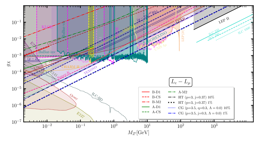
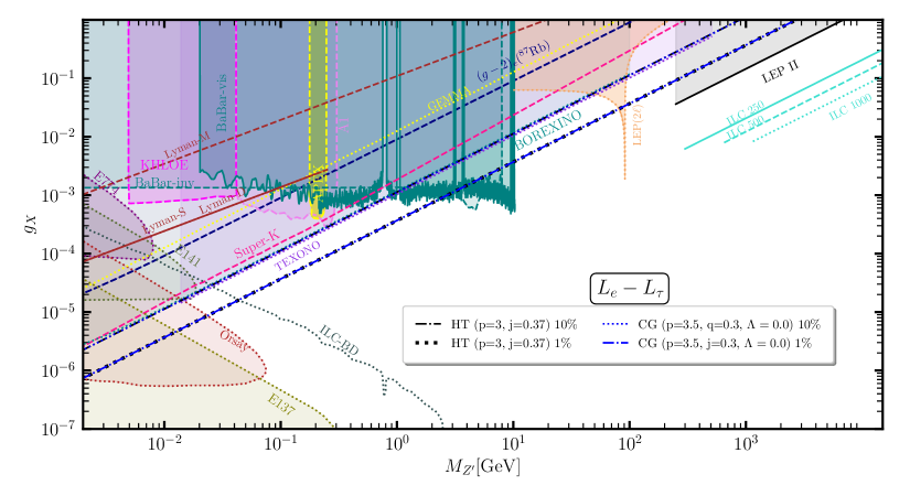
Figure 13: Limits on $g_{X}-M_{Z^{\prime}}$ plane for the $L_{e}-L_{\mu}$ (upper panel) and $L_{e}-L_{\tau}$ (lower) scenarios.

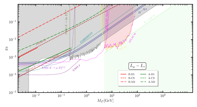
Figure 14: Limits on $g_{X}-M_{Z^{\prime}}$ plane for the $L_{\mu}-L_{\tau}$ scenario.

V.10 Limits from GRB

From GRB we have estimated the enhancement in energy deposition due to the influence of $Z^{\prime}$ using Schwarzchild, HT and modified gravity scenarios. The corresponding limits are given in Tab. 5 for different charges for the chiral scenarios like $U(1)_{X}$, $U(1)_{q+xu}$ and flavored scenarios like $B-3L_{i}$ and $L_{i}-L_{j}$ respectively. Hence we estimate constraints with $10\%$ and a prospective $1\%$ precision respectively. Following the constraints on the $U(1)$ from large VEV scenarios ($v_{\Phi}>v$), we estimate the bounds on $g_{X}-M_{Z^{\prime}}$ plane for different $U(1)$ scenarios. The bounds $M_{Z^{\prime}}/g_{X}$ will also satisfy the condition $v_{\Phi}>v$, therefore, bounds lower than that will not put any constraints on $g_{X}-M_{Z^{\prime}}$ plane. Applying this fact in Tab. 5 we find that in the case of general $U(1)_{X}$ scenario, GRB can not grant any limit from the Schwarzchild metric for $x_{H}=-1$ for $R^{\rm Sc}/M=3.67$, $x_{H}=0$ and $-1$ for $R^{\rm Sc}/M=5$ respectively. A similar scenario happens in the case of HT metric for $x_{H}=-1$ using $R^{\rm HT}/M=3$ and $J/M^{2}=0.37$ where as bounds obtained on $M_{Z^{\prime}}/g_{X}$ for different $x_{H}$ with $R^{\rm HT}/M=5$ and $J/M^{2}=0.37$ will not survive because all these values reside below the electroweak scale VEV. In the case of $U(1)_{q+xu}$ and $L_{e}-L_{\mu}$ scenarios using the same fact we notice that bounds for the Schwarzchild case with $R^{\rm Sc}/M=5$ and HT case with $R^{\rm HT}/M=5$, $J/M^{2}=0.37$ will not survive. Both the cases of $R/M$ values will bestow constraints in the $B-3L_{e}$ scenario, however, the bounds on $M_{Z^{\prime}}/g_{X}$ is stronger in HT case compared to the Schwarzchild case. Finally, we observe that for fixed charges bounds obtained from HT is slightly stronger than the Schwarzchild case, however, the limits will be close depending on $R/M$ and $J/M^{2}$ respectively. Therefore for simplicity, we show only bounds obtained using the HT case solving $`M_{Z^{\prime}}/g_{X}=\rm bounds$’ for $10^{-3}\rm{GeV}\leq M_{Z^{\prime}}\leq 25$ TeV where ‘bounds’ stands for the surviving values of this quantity given in Tab. 5 for $U(1)_{X}$ case, however, for the remaining cases we consider $10^{-3}\rm{GeV}\leq M_{Z^{\prime}}\leq 10$ TeV.

In the case of modified gravity, we consider CG and BIRN cases. As we explained, in the Schwarzchild and HT cases, in the same line we find that GRB can not constrain $x_{H}=-1$ in CG and BIRN cases for $R^{\rm CG}/M=3.5$, $q=0.3$, $I=0.0$ and $R^{\rm BIRN}/M=3$, $b/M=0.5$ in $U(1)_{X}$ scenario. Whereas in CG and BIRN cases GRB affects only $x_{H}=2$ in $U(1)_{X}$ scenario for $R^{\rm CG}/M=5$, $q=0.3$, $I=0.0$ and $R^{\rm CG}/M=5$, $q=0.5$, whereas rest of the cases show bounds on $M_{Z^{\prime}}/g_{X}$ which estimate VEV of the general $U(1)_{X}$ scenario lower than $v$. Due to this fact bounds obtained on $M_{Z^{\prime}}/g_{X}$ from CG and BIRN cases with $R^{\rm CG}/M=5$, $q=0.3$, $I=0.0$ and $R^{\rm CG}/M=5$, $q=0.5$ do not survive. Following the same approach for the $U(1)_{q+xu}$ scenario we find that estimated bounds on $M_{Z^{\prime}}/g_{X}$ using $R^{\rm CG}/M=3.5$, $q=0.3$, $I=0.0$ and $R^{\rm BIRN}/M=3$, $b/M=0.5$ for CG and BIRN cases respectively survive for all $x$, however, those estimated from the remaining choices do not survive due to the fact that they can not satisfy the condition $v_{\Phi}>v$. Among the flavor scenarios $B-3L_{e}$ scenario can be constrained from CG and BIRN cases for the required choices of parameters like $R/M$, $q$, $I$ and $b/M$ whereas in $L_{i}-L_{j}$ scenario constraints on $M_{Z^{\prime}}/g_{X}$ can be obtained from CG and BIRN cases using $R^{\rm CG}/M=3.5$, $q=0.3$, $I=0.0$ and $R^{\rm BIRN}/M=3$, $b/M=0.5$ respectively. The other choice will not be able to constrain $g_{X}-M_{Z^{\prime}}$ parameters because it does not satisfy $v_{\Phi}>v$. We find that constraints on $M_{Z^{\prime}}/g_{X}$ obtained from the CG scenario is slightly greater than those obtained using BIRN scenario. Therefore constraints on $g_{X}-M_{Z^{\prime}}$ obtained from CG scenario is slightly stronger than the BIRN case. As a result we show only the constraints in the final limit plots obtained from the CG case due to simplicity solving $`M_{Z^{\prime}}/g_{X}=\rm bounds$’ for $10^{-3}$ GeV $\leq M_{Z^{\prime}}\leq 10$ TeV where ‘bounds’ stands for the surviving values of this quantity given in Tab. 5 for different $U(1)$ extended scenarios.

Final limits are given in Figs. 9-12 for $U(1)_{X}$ and $U(1)_{q+Xu}$ cases. We show different existing bounds in $U(1)_{X}$ cases with colored lines and only relevant ones in case of $U(1)_{q+xu}$ with colored lines and remaining ones with gray shaded regions. We find that the strongest GRB contours obtained from the modified gravity model CG (blue dot and dot-dashed lines) are almost matching with the HT (black dot and dot-dashed lines) case. There is no limits for $x_{H}=-1$ in $U(1)_{X}$ case. The bounds are shown in the upper panel of Fig. 9. In case of $x=-1$ in $U(1)_{q+xu}$ scenario, given in the lower panel of the same figure, we find the bounds from the GRB scenarios belong to the gray shaded region. In Fig. 10 we show $x_{H}=0$ and $x=1$ from both $U(1)_{X}$ and $U(1)_{q+xu}$ scenarios representing the bounds on $g_{X}-M_{Z^{\prime}}$ plane for B$-$L scenario. We find that GRB contours with $10\%$ precision are comparable with the bounds obtained by BOREXINO, TEXONO and CHARM-II depending on $M_{Z^{\prime}}$. However, the bounds with prospective $1\%$ precision could provide a strong limit on the gauge coupling $6\times 10^{-6}\leq g_{X}\leq 7\times 10^{-5}$ for $0.025$ GeV $\leq M_{Z^{\prime}}\leq 0.25$ GeV. The prospective bounds with $1\%$ precision crosses the bounds obtained from the beam-dump scenarios at FASER, FASER2 and ILC-BD which could be tested in future. Limits on the $U(1)$ gauge coupling for $x_{H}=1$ and $x=0$ are shown in the upper and lower panels of Fig. 11 for $U(1)_{X}$ and $U(1)_{q+xu}$ respectively. We find that in $U(1)_{X}$ case prospective searches from FASER, FASER2 and ILC-BD could provide complementary search reaches to probe $Z^{\prime}$ around $0.06$ GeV. On the other hand limits from existing bounds, specially from $\nu-$cal covers the area where prospective searches could cross over in case of $U(1)_{q+xu}$ scenario. Bounds on the $U(1)$ gauge coupling for different $M_{Z^{\prime}}$ for $x_{H}(x)=2$ are shown in Fig. 12 in the lower and upper panels for $U(1)_{X}$ and $U(1)_{q+xu}$ respectively providing same experience like the previous charge assignment. We find that limits from dark photon searches at LHCb ($2.2$ GeV $\leq M_{Z^{\prime}}\leq 70$ GeV) and CMS ($1$ GeV $\leq M_{Z^{\prime}}\leq 9$ GeV) provide stronger limit than the other existing searches which occupy the parameter regions predicted by GRB. Finally we find that GRB contours could provide strong limits on the $g_{X}$ for a narrow range $100$ GeV $\leq M_{Z^{\prime}}\leq 150$ GeV for any charge of $U(1)_{X}$ and $U(1)_{q+xu}$ scenarios which could be probed by future collider experiments. We find that among the existing beam-dump scenarios $\nu-$cal provides the strongest bounds in case of $U(1)_{X}$ and $U(1)_{q+xu}$ scenarios. Other existing bounds from different beam-dump scenarios are shown by different colored lines for $U(1)_{X}$ case whereas by a collective gray shaded regions in case $U(1)_{q+xu}$ involving E774, NA64, E141, E137, Orsay, NoMad, PS191 and CHARM etc. BaBar(vis and invis) provides stronger bounds on $g_{X}-M_{Z^{\prime}}$ plane within $0.5$ GeV $\leq M_{Z^{\prime}}\leq 10$ GeV. We find that limits estimated from $(g-2)_{e}$ (Rb and CS) and $(g-2)_{\mu}$ are weak compared to the GRB bounds for different charges (expect $x_{H}(x)=-1$ where $g-2$ limits are negative electron and muon respectively) of the $U(1)_{X}$ and $U(1)_{q+xu}$ scenarios respectively. We also find that limits estimated from GEMMA and COHERENT experiments are weak compared to the GRB limits in case of $U(1)_{X}$ scenario, however, they belong to the gray shaded area in case of $U(1)_{q+xu}$ scenario, respectively. Limits from BaBaR(vis and invis) are weaker than scattering experiments like TEXONO, BOREXINO (belong to the gray shaded region in $U(1)_{q+xu}$) and dark photon searches from LHCb and CMS limits, respectively apart from a narrow window of $Z^{\prime}$ mass between $9$ GeV $\leq M_{Z^{\prime}}\leq 10$ GeV. Limits obtained from GRB with $10\%$ and $1\%$ precisions are weaker than the current LEP-II bounds for $M_{Z^{\prime}}>209$ GeV in general $U(1)$ scenarios for different charges. Prospective ILC bounds are stronger than the GRB bounds for $M_{Z^{\prime}}>\sqrt{s}_{\rm ILC}$.

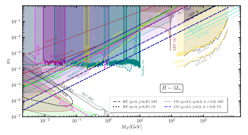
Figure 15: Limits on $g_{X}-M_{Z^{\prime}}$ plane for $B-3L_{e}$ scenario.

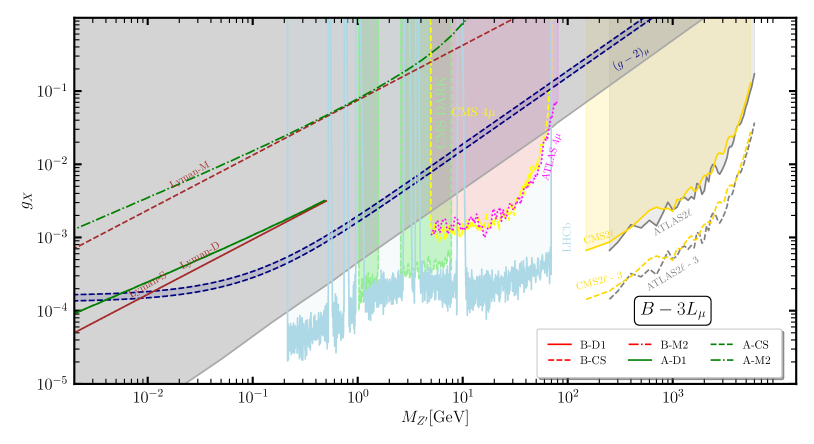
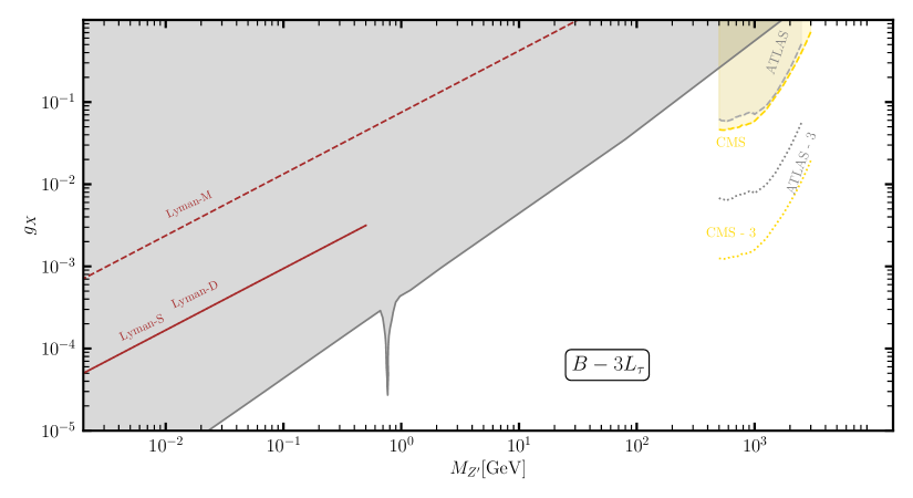
Figure 16: Limits on $g_{X}-M_{Z^{\prime}}$ plane for $B-3L_{\mu}$ (upper panel) and $B-3L_{\tau}$ (lower panel) scenarios.

Estimating bounds from GRB we find limits on the flavored scenarios like $L_{e}-L_{\mu}$ and $L_{e}-L_{\tau}$ scenarios in the upper and lower panels of Fig. 13. We find that limits from $10\%$ precision is comparable with TEXONO bounds for $L_{e}-L_{\mu}$ and $L_{e}-L_{\tau}$ scenarios. Whereas prospective bounds with $1\%$ precision could be stronger. The GRB contours with $10\%$ and $1\%$ precision cross the prospective ILC-BD line at $\{M_{Z^{\prime}},g_{X}\}=\{0.02\rm{GeV},2.5\times 10^{-5}\}$ and $\{0.05\rm{GeV},1.5\times 10^{-5}\}$, respectively. Like $U(1)_{X}$ and $U(1)_{q+xu}$ cases GRB contours could provide strong limits on the $g_{X}$ for a narrow range $100$ GeV $\leq M_{Z^{\prime}}\leq 150$ GeV. The $Z^{\prime}-$electron coupling is same in $L_{e}-L_{\mu}$ and $L_{e}-L_{\tau}$ cases causing same bounds where $Z^{\prime}-$electron interaction is involved. We find that in cases of $L_{i}-L_{j}$, Orsay and E137 provide stronger bound up to $\{M_{Z^{\prime}},g_{X}\}=\{0.08~{}\rm{GeV},10^{-6}\}$ and $\{0.25~{}\rm{GeV},10^{-7}\}$ respectively whereas E774 and E141 provide comparatively weaker bounds for $M_{Z^{\prime}}\leq 0.02$ GeV. Limits estimated from CHARM-II, GEMMA and BaBar(vis and invis for $M_{Z^{\prime}}\leq 0.02$ GeV) are weaker than the GRB bounds. Bounds obtained on $g_{X}$ for $Z\to 4\mu$ search in case of $L_{e}-L_{\mu}$ scenario provide stronger bound for $10$ GeV $\leq M_{Z^{\prime}}\leq 50$ GeV where $U(1)$ coupling varies between $0.003\leq g_{X}\leq 0.04$. There is no bound in this range for $L_{e}-L_{\tau}$ scenario because muon has no direct coupling with $Z^{\prime}$ in this case. Following the same line we provide bounds from CHARM-II in case of $L_{e}-L_{\mu}$ scenario. In addition to that we find constrains from [232] where $e^{-}e^{+}$ collision at KLOE experiment [253, 254] provide a stronger bound on $g_{X}$ for a narrow range $0.6$ GeV $\leq M_{Z^{\prime}}\leq 1$ GeV which can reach up to $4\times 10^{-4}\leq g_{X}\leq 3\times 10^{-4}$ touching the prospective bounds from GRB with $1\%$ precision at $\{M_{Z^{\prime}},g_{X}\}=\{1~{}\rm{GeV},2\times 10^{-4}\}$. The bounds obtained from KLOE are weaker compared to the other bounds in case of $L_{e}-L_{\tau}$ scenario. We show the limits [232] obtained from the APEX [155] and A1 [153, 152] experiments in case $L_{e}-L_{(\mu,\tau)}$ scenarios to be weak compared to the limits estimated for GRB. The $(g-2)_{\mu(e)}$ bounds for $L_{e}-L_{\mu(\tau)}$ scenario is weak compared to the GRB constraints. We find that GRB bounds with $10\%$ and prospective $1\%$ precision are stronger than the Super-K bounds obtained from [231]. Limits obtained from GRB with $10\%$ and $1\%$ precisions are weaker than the current LEP-II bounds for $M_{Z^{\prime}}>209$ GeV in case of $L_{e}-L_{\mu}$ and $L_{e}-L_{\tau}$ scenarios. Prospective ILC bounds are stronger than the GRB bounds for $M_{Z^{\prime}}>\sqrt{s}_{\rm ILC}$.

Bounds estimated from the GRB scenario in $B-3L_{e}$ case can be found in Fig. 15. The limit obtained with $10\%$ precision is comparable with the results obtained from TEXONO experiment. We find that for the $B-3L_{e}$ case, GEMMA provides limits around $6\times 10^{-6}\leq g_{X}\leq 10^{-4}$ for $0.03$ GeV $\leq M_{Z^{\prime}}\leq 0.3$ GeV which is comparable with the limits obtained from TEXONO and GRB with $10\%$ precision respectively, however, bounds obtained from the GRB analysis with a prospective $1\%$ precision could be a factor of five stronger than these bounds. Considering the limits from KOLE [253, 254], APEX [155], A1 [153, 152] and NA48/2 [154] experiments from [232, 231] which are weaker than the estimated GRB bounds. Limits obtained from GRB with $10\%$ precision are comparable with the current LEP-II bounds for $M_{Z^{\prime}}>209$ GeV whereas bounds with $1\%$ precision are stronger than the current LEP-II limits. Prospective ILC bounds are stronger than the GRB bounds for $M_{Z^{\prime}}>\sqrt{s}_{\rm ILC}$.

In flavored scenarios, we find that strongest bounds from GRB could also appear within $100$ GeV $\leq M_{Z^{\prime}}\leq 150$ GeV where corresponding $U(1)$ coupling varies between $0.02\leq g_{X}\leq 0.03$. When $Z^{\prime}$ is light such that $M_{Z^{\prime}}\simeq\mathcal{O}(0.01)$ GeV, the contours from GRB could intersect with the prospective limits from FASER, FASER2 (in $B-3L_{e}$ case only) and ILC-BD respectively which could be probed in future. We find that BaBar (vis and invis) provide stronger bounds for $M_{Z^{\prime}}\geq 0.3(0.11)$ GeV in case of $L_{e}-L_{\mu}$ scenario and $M_{Z^{\prime}}\geq 0.9(0.2)$ GeV in case of $L_{e}-L_{\tau}$ scenario, respectively compared to the bounds estimated from GRB using $10\%(1\%)$ precision, respectively. We find that in case of $B-3L_{e}$ scenario $\nu-$cal provides strongest bound among the existing beam-dump scenarios up to $M_{Z^{\prime}}\leq 0.3$ GeV. Prospective bounds from the beam-dump scenario from DUNE (DUNE-BD) are weaker than $\nu-$cal scenario for $M_{Z^{\prime}}\leq 0.27$ GeV.

V.11 Limits from blazars and AGN

The total cross section for $\nu$-DM scattering process depends on the mediator mass, here $M_{Z^{\prime}}$ and general $U(1)$ coupling, $g_{X}$ in addition to the neutrinos energies. In this analysis we will estimate constraints on these parameters. Therefore we write $\sigma=\sigma(g_{X},M_{Z^{\prime}})$ and the cascade equation given in Eq. 95 gets modified as

$$\frac{d\Phi}{dx}=-\sigma(g_{X},M_{Z^{\prime}})\frac{\Sigma(r)}{m_{\rm DM}}\;\Phi+\frac{\Sigma(r)}{m_{\rm DM}}\int_{E^{\prime}}^{\infty}dE\;\frac{d\sigma(g_{X},M_{Z^{\prime}})}{dE^{\prime}}\Phi(E)$$ (132)

using the fact $E_{\nu}^{2}+{E_{\nu}^{\prime}}^{2}>>m_{\rm DM}(E_{\nu}^{\prime}-E_{\nu})$ we use the following parametrization to solve the cascade equation

$$\alpha_{1}=\frac{g_{X}^{4}\;\Sigma}{8\pi M_{Z^{\prime}}^{4}}(1\;\text{TeV}),\;\;\alpha_{2}=\frac{m_{DM}}{M_{Z^{\prime}}^{2}}(1\;\text{TeV})$$ (133)

where $\alpha_{1,2}$ are dimensionless quantities. This parametrization will be used for the differential scattering cross-sections involving three types of DM candidates. The second term in Eq. 132 is proportional to the differential scattering cross section and it can be parameterized in terms of $\alpha_{1,2}$; hence, it can be written in terms of $\alpha_{1,2}$ and $m_{\rm DM}$. In our analysis, we fix $m_{\rm DM}$. Therefore this term depends on $\alpha_{1,2}$ only. To constrain the parameter space of $g_{X}$ and $M_{Z^{\prime}}$ using blazar and AGN event, we apply the following steps:

1. Using the initial flux of blazar and AGN given in Eqs. 96 and 100 respectively, we compute the final attenuated flux $\Phi_{\tilde{a}}$ by solving the cascade equation for different values of $\alpha_{1,2}$ which is equivalent to different values of $g_{X}$ and $M_{Z^{\prime}}$ related by Eq. 133.

2. Using Eq. 97 and $\Phi_{\tilde{a}}$ we calculate the expected number of events at IceCube for the attenuated flux corresponding to blazar and AGN.

3. Finally we require that the number of events be at least $10\%$ of the total observed events with no $\nu$-DM scattering (i.e 0.1 events in case of TXS 0506+056 and 3 events in case of AGN) for deriving a limit at $90\%$ C.L. on $g_{X}-M_{Z^{\prime}}$ plane.

Now we estimate constrains on $g_{X}-M_{Z^{\prime}}$ plane for chiral and flavored scenarios from the blazar and AGN cases considering $m_{\rm DM}=3M_{Z^{\prime}}$.

Constraints from blazar and AGN cases considering $x_{H}(x)=-1$, $0$, $1$ and $2$ for $U(1)_{X}$ (upper panel) and $U(1)_{q+xu}$ (lower panel) scenarios in Figs. 9- 12, respectively. We mention that $x_{H}=0$ and $x=1$ cases shown in Fig. 10 under $U(1)_{X}$ and $U(1)_{q+xu}$ scenarios resemble the B$-$L scenario. We denote the Dirac(D1) and complex scalar(CS) type DM candidates with $U(1)$ charge $Q_{\chi}=1000$ (under the perturbative limit $g|Q_{\chi}|\leq\sqrt{4\pi}$) and Majorana RHN DM (M2) with $U(1)$ charge $-5$. The blazar (B) scenarios for the corresponding D1, CS and M2 cases are represented by red solid (B-D1), dashed (B-CS) and dot-dashed (B-M2) lines whereas the AGN (A) scenarios are represented by corresponding green lines. The B-D1 (A-D1) and B-CS (A-CS) derive stronger limits which almost overlap with each other due to the fact that $E_{\nu}^{2}+{E_{\nu}^{\prime}}^{2}>>m_{\rm DM}(E_{\nu}^{\prime}-E_{\nu})$ and same $U(1)$ charges whereas the limits obtained from the Majorana DM are weaker compared to the Dirac and complex scalar cases due its different $U(1)$ charge. Among the blazar and AGN cases we obtain that AGN cases are stronger than the respective blazar cases. Comparing with existing bounds we find that limits obtained from the blazar and AGN scenarios are weak compared to the limits obtained from the scattering experiments like COHERENT, CHARM-II, GEMMA, BOREXINO, TEXONO and dark photon searches at BaBar(vis and invis), LHCb and CMS, respectively. The existing bounds from different beam-dump scenarios like NA64, E774 and E141 covers the region for $M_{Z^{\prime}}\leq 0.02$ GeV for the Dirac and CS cases with $Q_{\chi}=1000$, however, bounds from KEK, Orsay, NoMad, CHARM and E137 provide strong bound for $M_{Z^{\prime}}$ range under consideration. Among the beam-dump scenarios strongest existing bound comes from $\nu-$cal which is stronger than the prospective search reach for the beam-dump scenario at DUNE (DUNE-BD) for $M_{Z^{\prime}}\leq 0.4$ GeV. $\nu-$cal provides stronger bound than AGN (D1 and CS) cases for $M_{Z^{\prime}}\leq 0.002$ GeV. The crossovers of the AGN (D1 and CS) bounds with the prospective FASER, FASER2 and ILC-BD scenarios also appear in the sahded regions for both $U(1)_{X}$ and $U(1)_{q+xu}$ scenarios. We find that bounds obtained from GRB are roughly $\mathcal{O}(2)-\mathcal{O}(3)$ of magnitude stronger than the blazar and AGN bounds depending on $M_{Z^{\prime}}$.

We estimate bounds on the $g_{X}-M_{Z^{\prime}}$ plane for $L_{e}-L_{\mu}$ and $L_{\mu}-L_{\tau}$ scenarios constraining the $\nu-$DM scattering from blazar and AGN data observed by IceCube. The limits are shown in the upper panel of Fig. 13 for $L_{e}-L_{\mu}$ and in Fig. 14 for $L_{\mu}-L_{\tau}$ scenarios, respectively. We find that in $L_{e}-L_{\mu}$ scenario, limits from blazar and AGN are weaker than the estimated limits obtained from BaBar(vis and invis), CHARM-II, TEXONO, BOREXINO and GRB scenarios. On the other hand we find that limits obtained after studying Majorana DM from blazar (B-M2) and AGN (A-M2) are the weakest in these two scenarios. Limits estimated from B-D1, B-CS are also weak in the flavored scenarios. However, in case of $L_{\mu}-L_{\tau}$ scenario, A-D1 and A-CS are stronger than the $(g-2)_{\mu}$ limits for $M_{Z^{\prime}}\leq 0.02$ GeV. AGN scenario also provide a strong bound for the narrow range $0.0175$ GeV$\leq M_{Z^{\prime}}\leq 0.03$ GeV, however, limits for $M_{Z^{\prime}}\geq 0.03$ GeV belong to gray shaded region whose boundary consists of the strongest limits from BOREXINO, CCFR [255], BaBar 4$\mu$ [231] and $4\mu$ search from CMS [256] and ATLAS [257], respectively. It is interesting to notice that in case of $L_{\mu}-L_{\tau}$, limits obtained from white dwarf starts [258, 231] are stronger than BOREXINO. Remaining part of the boundary of the gray shaded region consists of CCFR and 4$\mu$ search from BaBar respectively. We find that $4\mu$ search from the CMS can constrain the parameter regions from $L_{e}-L_{\mu}$ and $L_{\mu}-L_{\tau}$ scenarios [256] providing bounds for $4$ GeV $\leq M_{Z^{\prime}}\leq 70$ GeV where limits on $g_{X}$ could reach up to $1.5\times 10^{-3}$ [256]. In case of $L_{\mu}-L_{\tau}$ we find that limits from new $(g-2)_{\mu}$ data provide strong bound on the gauge coupling within $4\times 10^{-4}\leq g_{X}\leq 10^{-3}$ for $0.01$ GeV $\leq M_{Z^{\prime}}\leq 0.2$ GeV where AGN could provide comparable limits from Dirac (D2) and complex scalar (CS) DM candidates, respectively. In addition to that bounds can be obtained on the gauge coupling from NA62 experiment using $K\to\mu+E_{T}^{\rm miss}$ mode following [259, 260, 261] which is stronger than the bounds obtained from $(g-2)_{\mu}$ experiment. Whereas bounds from NA62 using $K\to 3\mu+E_{T}^{\rm miss}$ is comparable to the bounds obtained from the $4\mu$ search from the BaBar experiment belonging to the gray shaded area. We find that a prospective limit from the Belle-II experiment at 50 $\rm{ab}^{-1}$ luminosity can vary within $3.2\times 10^{-4}\leq g_{X}\leq 1.6\times 10^{-3}$ for $0.007$ GeV $\leq M_{Z^{\prime}}\leq 5$ GeV [262]. Within this range, we find that limits obtained analysing AGN (D1 and CS) data comparing $\nu-$DM scattering could provide comparable bound for $M_{Z^{\prime}}=0.01$ GeV with prospective reach from Belle-II at 50 ab^-1 luminosity. Prospective sensitivities from NA64$\mu$ [263] and COHERENT [231] experiment could be stronger than the limits obtained analysing the AGN data for Dirac (D1) and complex scalar (CS) DM candidates.

We estimate limits on the $g_{X}-M_{Z^{\prime}}$ plane constraining $\nu-$DM scattering from blazar and AGN data observed by IceCube experiment in the context of $B-3L_{\mu}$ scenario. The limit plots are shown in the upper panel of Fig. 16. The gray-shaded region represents the strongest limits obtained by the neutrino Non-Standard Interaction (NSI) and it is taken from [30]. We show the estimated limits from the dark photon searches from LHCb, CMS experiments respectively. In addition to that we add limits obtained from the $4\mu$ search from CMS[256]. We find that limits obtained by constraining $\nu-$DM scattering using blazar and AGN results from IceCube are weaker than existing limits. We also estimate limits on the gauge coupling with respect to the $Z^{\prime}$ mass using latest $(g-2)_{\mu}$ data which belong to the grey-shaded region.

V.12 Theoretical limits from neutrino-DM scattering

We consider the theoretical limits on $\nu$-DM interaction. The interaction affects the Cosmic Microwave Background (CMB) spectrum. The effect parametrizes a dimensionless parameter

$$u_{\nu\rm DM}\equiv\frac{\sigma_{\nu\rm DM}}{\sigma_{\rm Th}}\left(\frac{m_{\rm DM}}{100{\rm GeV}}\right)^{-1}$$ (134)

where $\sigma_{\rm Th}$ is the Thomson scattering cross section and $\sigma_{\nu\rm DM}$ is the $\nu-$DM scattering cross section. We can obtain the upper bounds of the total cross-section for neutrino DM scattering from the Lyman-$\alpha$ data [90] as follows

$$\sigma_{\nu\rm DM}\left(\frac{m_{\rm DM}}{100{\rm GeV}}\right)^{-1} = \sigma_{\rm Th}u_{\nu\rm DM}<3.66\times 10^{-30}~{}{\rm cm^{2}}$$ (135)

Comparing the theoretically estimated cross sections with respect to the observed upper limit on the $\nu-$DM scattering cross section from the Lyman-$\alpha$ line, we estimate limits on the $U(1)$ gauge coupling with respect to $M_{Z^{\prime}}$ for the chiral and flavored scenarios. We find that in the chiral cases for different $x_{H}$ or $x$, Lyman-$\alpha$ line with Dirac and complex scalar DM candidates (Lyman-D and Lyman-S, respectively) match with each other due to large value of $Q_{\chi}$ and $E_{\nu}^{2}+{E_{\nu}^{\prime}}^{2}>>m_{\rm{DM}}(E_{\nu}^{\prime}-E_{\nu})$ under the perturbative limit $g|Q_{\chi}|<\sqrt{4\pi}$. The Majorana DM (Lyman-M) case is weak compared to the Dirac (D) and complex scalar (S) cases. Through out the chiral cases Lyman-$\alpha$ (Lyman-M, Lyman-D and Lyman-S) lines are weak compared to the limits obtained from the scattering experiment, beam-dump experiment and limits obtained from GRB scenarios (current precesion with $10\%$ and prospective precision with $1\%$) shown in Figs. 9-12.

We find the above behavior of the Lyman lines in the case of $L_{e}-L_{\mu}$ and $L_{e}-L_{\tau}$ scenarios shown in the upper and lower panels of Fig. 13. Significant difference occurs in the $L_{\mu}-L_{\tau}$ scenario as shown in Fig. 14. Under the perturbative constraints we find that limits obtained from the Lyman-D and Lyman-S scenarios could provide the strongest bound on the $U(1)$ gauge coupling for $0.004$ GeV $\leq M_{Z^{\prime}}\leq 0.06$ GeV. Bounds estimated from considering Majorana DM candidate represented by Lyman-M are lying in the grsay shaded region. Limits from Lyman-D and Lyman-S could be comparable with the bounds obtained from NA62 experiment considering $K\to\mu+E_{T}^{\rm miss}$, $(g-2)_{\mu}$ and prospective bounds from COHERENT, NA64$\mu$ and Belle-II. These bounds could be probed by different experiments in near future. In the context of $L_{\mu}-L_{\tau}$ scenario, the shaded region in green is disfavored if we want to explain $b\to s\mu^{+}\mu^{-}$ anomalies [264].

We show that estimated bounds obtained from the case of $B-3L_{i}$ scenario are shown in Figs. 15 and Fig. 16 respectively. Like the chiral cases, in this flavored scenario, limits obtained from Lyman-M are weaker than Lyman-D and Lyman-S, however, all the lines belong to the gray-shaded region.

VI Conclusions

In this paper, we consider chiral and flavored scenarios where interactions of $Z^{\prime}$ depend on the corresponding $U(1)$ charges of the fermions. We incorporate cosmic bursts involving GRB 221009A which is the brightest GRB of all time, cosmic blazar (TXS 0506+056) and AGN (NGC 1068) to probe neutrino interactions with $Z^{\prime}$ from different models. In the context of GRB, we study electron-positron pair production from neutrino anti-neutrino interaction involving SM and $Z^{\prime}$ gauge boson. Estimating energy deposition of SM and BSM process involving Sc, HT and modified gravity scenarios (BRIN and CG) we constrain $U(1)$ gauge coupling with respect to $Z^{\prime}$ mass on $g_{X}-M_{Z^{\prime}}$ plane. As a part of chiral aspects, we used $U(1)_{X}$ and $U(1)_{q+xu}$ scenarios where we changed the corresponding charges to estimate bounds. We found that for $x_{H}=-1$, no bounds from GRB could be obtained from the fact that the estimated VEV of $U(1)_{X}$ scenario will be lower than electroweak VEV which is not possible in our model set-up. In addition to that we find estimated bounds with $10\%$ precision are comparable with TEXONO results. Prospective bounds with $1\%$ precision are stronger than the previous cases in the case of $U(1)_{X}$ and $U(1)_{q+xu}$ scenarios which cross over prospective bounds from FASER, FASER2 and ILC-BD which could be verified in future. A similar inference could be drawn for the $L_{e}-L_{\mu,\tau}$, $B-3L_{e}$ scenarios where FASER, FASER2, beam-dump search at ILC could be interesting to probe a parameter space favoured by GRB depending on the interaction between $Z^{\prime}$ and the SM fermions. To study neutrino interactions from blazars and AGN we use IceCube data in the context of $\nu-$DM scattering which could probe light $Z^{\prime}$ providing bounds on $g_{X}-M_{Z^{\prime}}$ plane for different models. We introduced complex scalar, Dirac and Majorana DM candidates with respective $U(1)$ charges under the perturbative limit. We find that in case of $L_{\mu}-L_{\tau}$ scenario $\nu-DM$ scattering compared with IceCube data could provide strong bounds for $0.006$ GeV $\leq M_{Z^{\prime}}\leq 0.02$ GeV where bounds on $U(1)$ coupling could vary between $3\times 10^{-4}\leq g_{X}\leq 7\times 10^{-4}$. These bounds are comparable with recent $(g-2)_{\mu}$ observation and bounds obtained by COHERENT $\mu-$nucleon scattering. Belle-II, NA62 and NA64_μ experiments could probe this parameter region in the future. We also find the theoretical limits on $\nu-$DM scattering comparing with Lyman-$\alpha$ line for Dirac and complex scalar DM candidates in the context of $L_{\mu}-L_{\tau}$ scenario which could provide strong limits for $0.004$ GeV $\leq M_{Z^{\prime}}\leq 0.08$ GeV where the corresponding gauge coupling will vary between $1.75\times 10^{-4}\leq g_{X}\leq 8\times 10^{-4}$ under perturbative limit which could be probed by NA62, Belle-II and NA64$\mu$ experiments in future.

Appendix A Cross sections of $\nu\bar{\nu}\to e^{-}e^{+}$ process in center of mass frame in general $U(1)$ scenarios:

A.1 Kinematics

We define the quantities $p_{1}$ as initial neutrino momentum, $p_{2}$ as initial anti-neutrino momentum, $k_{1}$ as final charged lepton momentum, $k_{2}$ as final charged lepton momentum. The $4-$vector representation of these momenta are $p_{1}=(E,0,0,E)$, $p_{2}=(E,0,0,-E)$, $k_{1}=(E,0,E\sin\theta,E\cos\theta)$ and $k_{2}=(E,0,-E\sin\theta,-E\cos\theta)$. The scalar products and neutrino energy in laboratory frame are given by $k_{1}\cdot p_{1}=k_{2}\cdot p_{2}=E^{2}(1-cos\theta)$ and $k_{1}\cdot p_{2}=k_{2}\cdot p_{1}=E^{2}(1+cos\theta)$.

A.2 Amplitudes and Cross sections of $\nu_{e}\bar{\nu}_{e}\to e^{-}e^{+}$

We use the following gauge interactions,

$${\cal L}_{gauge}=Z^{\mu}\left(\bar{\nu}_{L}c_{L}^{\nu}\gamma_{\mu}\nu_{L}+\sum_{i=L,R}\bar{e}_{i}c_{i}^{e}\gamma_{\mu}e_{i}\right)+\left(W^{+\mu}\bar{\nu}_{L}c_{+}\gamma_{\mu}e_{L}+h.c.\right)+Z^{\prime\mu}\left(\bar{\nu}_{L}{\tilde{c}}_{L}^{\nu}\gamma_{\mu}\nu_{L}+\sum_{i=L,R}\bar{e}_{i}{\tilde{c}}_{i}^{e}\gamma_{\mu}e_{i}\right)$$ (136)

where $\{L,R\}$ are the projections and $\{c_{i}^{e},\tilde{c}_{i}^{e}\}$ are the corresponding couplings. The amplitudes for $\nu\bar{\nu}\rightarrow e^{+}e^{-}$ are given by

$$i{\cal M}_{1} = \frac{-ic_{\pm}^{2}}{M_{W}^{2}}\bar{v}(k_{1})\gamma_{\mu}P_{L}u(p_{1})\bar{u}(p_{2})\gamma^{\mu}P_{L}v(k_{2}),$$

$$i{\cal M}_{2} = \frac{ic_{L}^{\nu}}{M_{Z}^{2}}\bar{v}(p_{2})\gamma_{\mu}P_{L}u(p_{1})\bar{u}(k_{1})\gamma^{\mu}\left(c_{L}^{e}P_{L}+c_{R}^{e}P_{R}\right)v(k_{2}),$$

$$i{\cal M}_{3} = \frac{ic_{L}^{\nu}}{M_{Z^{\prime}}^{2}}\bar{v}(p_{2})\gamma_{\mu}P_{L}u(p_{1})\bar{u}(k_{1})\gamma^{\mu}\left(\tilde{c}_{L}^{e}P_{L}+\tilde{c}_{R}^{e}P_{R}\right)v(k_{2}),$$ (137)

where ${\cal M}_{1}$, ${\cal M}_{2}$ and ${\cal M}_{3}$ are amplitudes for the $W$, $Z$ and $Z^{\prime}$ mediated processes in Fig.2. The square of the amplitudes are given by

$$\frac{1}{4}\sum_{spin}\left|{\cal M}_{1}\right|^{2} = \frac{4c_{\pm}^{4}}{M_{W}^{4}}(k_{1}\cdot p_{2})(p_{1}\cdot k_{2}),$$

$$\frac{1}{4}\sum_{spin}\left|{\cal M}_{2}\right|^{2} = \frac{4c_{L}^{\nu 2}(c_{L}^{e2}+c_{R}^{e2})}{M_{Z}^{4}}(k_{1}\cdot p_{2})(p_{1}\cdot k_{2}),$$

$$\frac{1}{4}\sum_{spin}\left|{\cal M}_{3}\right|^{2} = \frac{4\tilde{c}_{L}^{\nu 2}(\tilde{c}_{L}^{e2}+\tilde{c}_{R}^{e2})}{M_{Z^{\prime}}^{4}}(k_{1}\cdot p_{2})(p_{1}\cdot k_{2}),$$ (138)

and the cross terms are given by

$$\frac{1}{4}\sum_{spin}\left({\cal M}_{1}{\cal M}_{2}^{\ast}+{\cal M}_{1}^{\ast}{\cal M}_{2}\right) = \frac{4c_{\pm}^{2}c_{L}^{\nu}c_{L}^{e}}{M_{W}^{2}M_{Z}^{2}}(k_{1}\cdot p_{2})(p_{1}\cdot k_{2}),$$

$$\frac{1}{4}\sum_{spin}\left({\cal M}_{1}{\cal M}_{3}^{\ast}+{\cal M}_{1}^{\ast}{\cal M}_{3}\right) = \frac{4c_{\pm}^{2}\tilde{c}_{L}^{\nu}\tilde{c}_{L}^{e}}{M_{W}^{2}M_{Z^{\prime}}^{2}}(k_{1}\cdot p_{2})(p_{1}\cdot k_{2}),$$

$$\frac{1}{4}\sum_{spin}\left({\cal M}_{2}{\cal M}_{3}^{\ast}+{\cal M}_{2}^{\ast}{\cal M}_{3}\right) = \frac{4c_{L}^{\nu}\tilde{c}_{L}^{\nu}(c_{L}^{e}\tilde{c}_{L}^{2}+c_{R}^{e}\tilde{c}_{R}^{2})}{M_{Z}^{2}M_{Z^{\prime}}^{2}}(k_{1}\cdot p_{2})(p_{1}\cdot k_{2}).$$ (139)

The total cross section is given by $\sigma v_{rel}=\frac{1}{64\pi E^{2}}\int d\cos\theta\overline{\sum(|{\cal M}_{i}|^{2}+|{\cal M}_{j}|^{2}+{\cal M}_{i}{\cal M}_{j}^{\ast}+{\cal M}_{i}^{\ast}{\cal M}_{j})}$ which reduces to

$$\sigma v_{rel}=\frac{E^{2}}{6\pi}\left(\frac{c_{\pm}^{4}}{M_{W}^{4}}+\frac{c_{L}^{\nu 2}(c_{L}^{e2}+c_{R}^{e2})}{M_{Z}^{4}}+\frac{\tilde{c}_{L}^{\nu 2}(\tilde{c}_{L}^{e2}+\tilde{c}_{R}^{e2})}{M_{Z^{\prime}}^{4}}+\frac{c_{\pm}^{2}c_{L}^{\nu}c_{L}^{e}}{M_{W}^{2}M_{Z}^{2}}+\frac{c_{\pm}^{2}\tilde{c}_{L}^{\nu}\tilde{c}_{L}^{e}}{M_{W}^{2}M_{Z^{\prime}}^{2}}+\frac{c_{L}^{\nu}\tilde{c}_{L}^{\nu}(c_{L}^{e}\tilde{c}_{L}^{\nu}+c_{R}^{e}\tilde{c}_{R}^{\nu})}{M_{Z}^{2}M_{Z^{\prime}}^{2}}\right).$$ (140)

A.3 Cross sections of $\nu_{\mu,\tau}\bar{\nu}_{\mu,\tau}\to e^{-}e^{+}$

If neutrino is not $\nu_{e}$, ${\cal M}_{1}=0$. Therefore, the total cross section is given by

$$\sigma v_{rel}=\frac{E^{2}}{6\pi}\left(\frac{c_{L}^{\nu 2}(c_{L}^{e2}+c_{R}^{e2})}{M_{Z}^{4}}+\frac{\tilde{c}_{L}^{\nu 2}(\tilde{c}_{L}^{e2}+\tilde{c}_{R}^{e2})}{M_{Z^{\prime}}^{4}}+\frac{c_{L}^{\nu}\tilde{c}_{L}^{\nu}(c_{L}^{e}\tilde{c}_{L}^{\nu}+c_{R}^{e}\tilde{c}_{R}^{\nu})}{M_{Z}^{2}M_{Z^{\prime}}^{2}}\right).$$ (141)

Appendix B $\nu-$DM scattering cross sections in laboratory frame in general $U(1)$ scenarios:

B.1 Kinematics

We define the quantities $p_{1}$ as initial neutrino momentum, $p_{2}$ as initial DM momentum, $k_{1}$ as final neutrino momentum, $k_{2}$ as final DM momentum. The $4-$vector representation of these momenta are $p_{1}=(E_{\nu}^{\prime},0,0,E_{\nu}^{\prime})$, $p_{2}=(m_{\chi},0,0,0)$, $k_{1}=(E_{\nu},0,E_{\nu}\sin\theta,E_{\nu}\cos\theta)$ and $k_{2}=(E_{\chi},0,-E_{\nu}\sin\theta,E_{\nu}^{\prime}-E_{\nu}\cos\theta)$ where $E_{\chi}=E_{\nu}^{\prime}+m_{\chi}-E_{\nu}$. The scalar products and neutrino energy in laboratory frame are given by $k_{1}\cdot p_{1}=E_{\nu}^{\prime}E_{\nu}(1-\cos\theta)$, $k_{1}\cdot p_{2}=m_{\chi}E_{\nu}$, $k_{2}\cdot p_{1}=m_{\chi}E_{\nu}^{\prime}-E_{\nu}^{\prime}E_{\nu}(1-\cos\theta)$, $E_{\nu}=\frac{m\chi E_{\nu}^{\prime}}{m_{\chi}+E_{\nu}^{\prime}(1-\cos\theta)}$.

B.2 Dirac fermion DM

We use the following gauge interactions,

$${\cal L}_{z^{\prime}}=Z^{\prime}_{\mu}\left(\bar{\nu}_{L}g_{\nu}\gamma_{\mu}\nu_{L}+\tilde{g}_{\chi}\bar{\chi}\gamma_{\mu}\chi\right)$$ (142)

where $g_{\nu}=g_{X}Q_{\ell}$ and $\tilde{g}_{\chi}=g_{X}Q_{\chi}$. The amplitude for $\nu DM\rightarrow\nu DM$ are given by

$$i{\cal M}=\frac{i\tilde{g}_{\chi}g_{\nu}}{(p_{1}-k_{1})^{2}-M_{Z^{\prime}}^{2}+i\Gamma_{Z^{\prime}}M_{Z^{\prime}}}\bar{u}(k_{1})\gamma_{\mu}u(p_{1})\bar{u}(k_{2})\gamma^{\mu}u(p_{2}).$$ (143)

The square of the amplitude is given by

$$\frac{1}{4}\sum_{spins}\left|{\cal M}\right|^{2}=\frac{4g_{\nu}^{2}\tilde{g}_{\chi}^{2}}{((p_{1}-k_{1})^{2}-M_{Z^{\prime}}^{2})^{2}+\Gamma_{Z^{\prime}}^{2}M_{Z^{\prime}}^{2}}\left((k_{1}\cdot k_{2})(p_{1}\cdot p_{2})+(k_{1}\cdot p_{2})(p_{1}\cdot k_{2})-m_{\chi}^{2}(k_{1}\cdot p_{1})\right).$$ (144)

The differential cross section is given by

$$\frac{d\sigma}{dE_{\nu}}=\frac{g_{\nu}^{2}\tilde{g}_{\chi}^{2}m_{\chi}}{8\pi E_{\nu}^{\prime 2}\{\left(2m_{\chi}(E_{\nu}^{\prime}-E_{\nu})+M_{Z^{\prime}}^{2}\right)^{2}+\Gamma_{Z^{\prime}}^{2}M_{Z^{\prime}}^{2}\}}\left(E_{\nu}^{\prime 2}+E_{\nu}^{2}-m_{\chi}(E_{\nu}^{\prime}-E_{\nu})\right).$$ (145)

The total cross section is given by

$$\sigma=\frac{g_{\nu}^{2}\tilde{g}_{\chi}^{2}m_{\chi}}{8\pi E_{\nu}^{\prime 2}}\int_{-1}^{1}d\cos\theta\frac{\left(E_{\nu}^{\prime 2}+E_{\nu}^{2}-m_{\chi}(E_{\nu}^{\prime}-E_{\nu})\right)}{\left(2m_{\chi}(E_{\nu}^{\prime}-E_{\nu})+M_{Z^{\prime}}^{2}\right)^{2}+\Gamma_{Z^{\prime}}^{2}M_{Z^{\prime}}^{2}}.$$ (146)

B.3 Majorana fermion DM

We use the following gauge interactions,

$${\cal L}_{Z^{\prime}}=Z^{\prime}_{\mu}\left(\bar{\nu}_{L}g_{\nu}\gamma_{\mu}\nu_{L}+\tilde{g}_{\chi}\bar{\chi}\gamma_{\mu}\gamma_{5}\chi\right),$$ (147)

The amplitude for $\nu DM\rightarrow\nu DM$ are given by

$$i{\cal M}=\frac{ig_{\nu}\tilde{g}_{\chi}}{(p_{1}-k_{1})^{2}-M_{Z^{\prime}}^{2}+i\Gamma_{Z^{\prime}}M_{Z^{\prime}}}\bar{u}(k_{1})\gamma_{\mu}u(p_{1})\bar{u}(k_{2})\gamma^{\mu}\gamma_{5}u(p_{2}).$$ (148)

The square of the amplitude is given by

$$\frac{1}{4}\sum_{spin}\left|{\cal M}\right|^{2}=\frac{4g_{\nu}^{2}\tilde{g}_{\chi}^{2}}{((p_{1}-k_{1})^{2}-M_{Z^{\prime}}^{2})^{2}+\Gamma_{Z^{\prime}}^{2}M_{Z^{\prime}}^{2}}\left((k_{1}\cdot k_{2})(p_{1}\cdot p_{2})+(k_{1}\cdot p_{2})(p_{1}\cdot k_{2})-m_{\chi}^{2}(k_{1}\cdot p_{1})\right).$$ (149)

The differential cross section is given by

$$\frac{d\sigma}{dE_{\nu}}=\frac{g_{\nu}^{2}\tilde{g}_{\chi}^{2}m_{\chi}}{8\pi E_{\nu}^{\prime 2}\{\left(2m_{\chi}(E_{\nu}^{\prime}-E_{\nu})+M_{Z^{\prime}}^{2}\right)^{2}+\Gamma_{Z^{\prime}}^{2}M_{Z^{\prime}}^{2}\}}\left(E_{\nu}^{\prime 2}+E_{\nu}^{2}-m_{\chi}(E_{\nu}^{\prime}-E_{\nu})\right).$$ (150)

The total cross section is given by

$$\sigma=\frac{g_{\nu}^{2}\tilde{g}_{\chi}^{2}m_{\chi}}{8\pi E_{\nu}^{\prime 2}}\int_{-1}^{1}d\cos\theta\frac{\left(E_{\nu}^{\prime 2}+E_{\nu}^{2}-m_{\chi}(E_{\nu}^{\prime}-E_{\nu})\right)}{\left(2m_{\chi}(E_{\nu}^{\prime}-E_{\nu})+M_{Z^{\prime}}^{2}\right)^{2}+\Gamma_{Z^{\prime}}^{2}M_{Z^{\prime}}^{2}}.$$ (151)

B.4 Complex scalar DM

We use the following gauge interactions,

$${\cal L}_{Z^{\prime}}=Z^{\prime}_{\mu}\left(\bar{\nu}_{L}g_{\nu}\gamma_{\mu}\nu_{L}+\tilde{g}_{\chi}(\chi^{*}\partial_{\mu}\chi-\partial_{\mu}\chi^{*}\chi\right),$$ (152)

The amplitude for $\nu DM\rightarrow\nu DM$ are given by

$$i{\cal M}=\frac{ig_{\nu}\tilde{g}_{\chi}}{(p_{1}-k_{1})^{2}-M_{Z^{\prime}}^{2}+i\Gamma_{Z^{\prime}}M_{Z^{\prime}}}\bar{u}(k_{1})\gamma_{\mu}P_{L}u(p_{1})(k_{2}+p_{2})^{\mu}.$$ (153)

The square of the amplitude is given by

$$\frac{1}{2}\sum_{spin}\left|{\cal M}\right|^{2}=\frac{1}{2}\frac{g_{\nu}^{2}\tilde{g}_{\chi}^{2}}{((p_{1}-k_{1})^{2}-M_{Z^{\prime}}^{2})^{2}+\Gamma_{Z^{\prime}}^{2}M_{Z^{\prime}}^{2}}\left(2(k_{1}\cdot k_{2}+k_{1}\cdot p_{2})(p_{1}\cdot k_{2}+p_{1}\cdot p_{2})-(k_{2}+p_{2})^{2}(k_{1}\cdot p_{1})\right).$$ (154)

The differential cross section is given by

$$\frac{d\sigma}{dE_{\nu}}=\frac{g_{\nu}^{2}\tilde{g}_{\chi}^{2}m_{\chi}}{8\pi E_{\nu}^{\prime 2}\{\left(2m_{\chi}(E_{\nu}^{\prime}-E_{\nu})+M_{Z^{\prime}}^{2}\right)^{2}+\Gamma_{Z^{\prime}}^{2}M_{Z^{\prime}}^{2}\}}\left(2E_{\nu}^{\prime}E_{\nu}-m_{\chi}(E_{\nu}^{\prime}-E_{\nu})\right).$$ (155)

The total cross section is given by

$$\sigma=\frac{g_{\nu}^{2}\tilde{g}_{\chi}^{2}}{8\pi E_{\nu}^{\prime 2}}\int_{-1}^{1}d\cos\theta\frac{E_{\nu}^{2}\left(2E_{\nu}^{\prime}E_{\nu}-m_{\chi}(E_{\nu}^{\prime}-E_{\nu})\right)}{\left(2m_{\chi}(E_{\nu}^{\prime}-E_{\nu})+M_{Z^{\prime}}^{2}\right)^{2}+\Gamma_{Z^{\prime}}^{2}M_{Z^{\prime}}^{2}}.$$ (156)

For light $Z^{\prime}$, $\Gamma_{Z}^{\prime}M_{Z^{\prime}}$ term in the denominators could be suppressed.

References

- [1] Particle Data Group Collaboration, P. A. Zyla et al., “Review of Particle Physics,” PTEP 2020 no. 8, (2020) 083C01.
- [2] G. Bertone, D. Hooper, and J. Silk, “Particle dark matter: Evidence, candidates and constraints,” Phys. Rept. 405 (2005) 279–390, arXiv:hep-ph/0404175.
- [3] Planck Collaboration, N. Aghanim et al., “Planck 2018 results. VI. Cosmological parameters,” Astron. Astrophys. 641 (2020) A6, arXiv:1807.06209 [astro-ph.CO]. [Erratum: Astron.Astrophys. 652, C4 (2021)].
- [4] Fermi-LAT Collaboration, M. Ackermann et al., “Constraining Dark Matter Models from a Combined Analysis of Milky Way Satellites with the Fermi Large Area Telescope,” Phys. Rev. Lett. 107 (2011) 241302, arXiv:1108.3546 [astro-ph.HE].
- [5] Fermi-LAT Collaboration, A. A. Abdo et al., “Constraints on Cosmological Dark Matter Annihilation from the Fermi-LAT Isotropic Diffuse Gamma-Ray Measurement,” JCAP 04 (2010) 014, arXiv:1002.4415 [astro-ph.CO].
- [6] P. Minkowski, “ at a Rate of One Out of Muon Decays?,” Phys. Lett. B 67 (1977) 421–428.
- [7] T. Yanagida, “Horizontal gauge symmetry and masses of neutrinos,” Conf. Proc. C 7902131 (1979) 95–99.
- [8] M. Gell-Mann, P. Ramond, and R. Slansky, “Complex Spinors and Unified Theories,” Conf. Proc. C 790927 (1979) 315–321, arXiv:1306.4669 [hep-th].
- [9] R. N. Mohapatra and G. Senjanovic, “Neutrino Mass and Spontaneous Parity Nonconservation,” Phys. Rev. Lett. 44 (1980) 912.
- [10] J. Schechter and J. W. F. Valle, “Neutrino Masses in SU(2) x U(1) Theories,” Phys. Rev. D22 (1980) 2227.
- [11] S. Weinberg, “Baryon and Lepton Nonconserving Processes,” Phys. Rev. Lett. 43 (1979) 1566–1570.
- [12] A. Davidson, “ as the fourth color within an model,” Phys. Rev. D 20 (1979) 776.
- [13] A. Davidson, M. Koca, and K. C. Wali, “U(1) as the Minimal Horizontal Gauge Symmetry,” Phys. Rev. Lett. 43 (1979) 92.
- [14] R. E. Marshak and R. N. Mohapatra, “Quark - Lepton Symmetry and B-L as the U(1) Generator of the Electroweak Symmetry Group,” Phys. Lett. 91B (1980) 222–224.
- [15] R. N. Mohapatra and R. E. Marshak, “Local B-L Symmetry of Electroweak Interactions, Majorana Neutrinos and Neutron Oscillations,” Phys. Rev. Lett. 44 (1980) 1316–1319. [Erratum: Phys. Rev. Lett.44,1643(1980)].
- [16] A. Das, N. Okada, and D. Raut, “Enhanced pair production of heavy Majorana neutrinos at the LHC,” Phys. Rev. D97 no. 11, (2018) 115023, arXiv:1710.03377 [hep-ph].
- [17] K. Chakraborty, A. Das, S. Goswami, and S. Roy, “Constraining general U(1) interactions from neutrino-electron scattering measurements at DUNE near detector,” JHEP 04 (2022) 008, arXiv:2111.08767 [hep-ph].
- [18] K. Asai, A. Das, J. Li, T. Nomura, and O. Seto, “Probing for chiral gauge boson through scattering measurement experiments,” arXiv:2307.09737 [hep-ph].
- [19] K. Asai, A. Das, J. Li, T. Nomura, and O. Seto, “Chiral Z’ in FASER, FASER2, DUNE, and ILC beam dump experiments,” Phys. Rev. D 106 no. 9, (2022) 095033, arXiv:2206.12676 [hep-ph].
- [20] M. Hashimoto, S. Iso, and Y. Orikasa, “Radiative symmetry breaking from flat potential in various U(1)’ models,” Phys. Rev. D 89 no. 5, (2014) 056010, arXiv:1401.5944 [hep-ph].
- [21] T. Appelquist, B. A. Dobrescu, and A. R. Hopper, “Nonexotic Neutral Gauge Bosons,” Phys. Rev. D 68 (2003) 035012, arXiv:hep-ph/0212073.
- [22] M. Carena, A. Daleo, B. A. Dobrescu, and T. M. P. Tait, “ gauge bosons at the Tevatron,” Phys. Rev. D70 (2004) 093009, arXiv:hep-ph/0408098 [hep-ph].
- [23] R. Foot, “New Physics From Electric Charge Quantization?,” Mod. Phys. Lett. A 6 (1991) 527–530.
- [24] X. G. He, G. C. Joshi, H. Lew, and R. R. Volkas, “NEW Z-prime PHENOMENOLOGY,” Phys. Rev. D 43 (1991) 22–24.
- [25] X.-G. He, G. C. Joshi, H. Lew, and R. R. Volkas, “Simplest Z-prime model,” Phys. Rev. D 44 (1991) 2118–2132.
- [26] W. Altmannshofer, S. Gori, M. Pospelov, and I. Yavin, “Neutrino Trident Production: A Powerful Probe of New Physics with Neutrino Beams,” Phys. Rev. Lett. 113 (2014) 091801, arXiv:1406.2332 [hep-ph].
- [27] A. Dasgupta, P. S. B. Dev, T. Han, R. Padhan, S. Wang, and K. Xie, “Searching for Heavy Leptophilic : from Lepton Colliders to Gravitational Waves,” arXiv:2308.12804 [hep-ph].
- [28] H.-S. Lee and E. Ma, “Gauged origin of Parity and its implications,” Phys. Lett. B 688 (2010) 319–322, arXiv:1001.0768 [hep-ph].
- [29] L. N. Chang, O. Lebedev, W. Loinaz, and T. Takeuchi, “Constraints on gauged B - 3 L(tau) and related theories,” Phys. Rev. D 63 (2001) 074013, arXiv:hep-ph/0010118.
- [30] M. Bauer, P. Foldenauer, and M. Mosny, “Flavor structure of anomaly-free hidden photon models,” Phys. Rev. D 103 no. 7, (2021) 075024, arXiv:2011.12973 [hep-ph].
- [31] D. Eichler, M. Livio, T. Piran, and D. N. Schramm, “Nucleosynthesis, Neutrino Bursts and Gamma-Rays from Coalescing Neutron Stars,” Nature 340 (1989) 126–128.
- [32] H. A. Bethe and J. R. Wilson, “Revival of a stalled supernova shock by neutrino heating,” Astrophys. J. 295 (1985) 14–23.
- [33] J. Cooperstein, L. van den Horn, and E. A. Baron, “Neutrino flows in collapsing stars: a two-fluid model,” ApJ 309 (1986) 653.
- [34] J. Cooperstein, L. J. van den Horn, and E. A. Baron, “Neutrino Pair Energy Deposition in Supernovae,” ApJ 321 (1987) L129.
- [35] J. Goodman, A. Dar, and S. Nussinov, “Neutrino Annihilation in type II Supernovae,” Astrophys. J. Lett. 314 (1987) L7–L10.
- [36] D. Eichler, M. Livio, T. Piran, and D. N. Schramm, “Nucleosynthesis, neutrino bursts and -rays from coalescing neutron stars,” Nature (London) 340 no. 6229, (July, 1989) 126–128.
- [37] M. Jaroszynski, “Neutrino Emission and Annihilation Near Tori around Black Holes,” Acta Astron. 43 (July, 1993) 183–191.
- [38] A. R. Prasanna and S. Goswami, “Energy deposition due to neutrino pair annihilation near rotating neutron stars,” Phys. Lett. B 526 (2002) 27–33, arXiv:astro-ph/0109058.
- [39] J. D. Salmonson and J. R. Wilson, “General relativistic augmentation of neutrino pair annihilation energy deposition near neutron stars,” Astrophys. J. 517 (1999) 859–865, arXiv:astro-ph/9908017.
- [40] J. D. Salmonson and J. R. Wilson, “Neutrino annihilation between binary neutron stars,” Astrophys. J. 561 (2001) 950–956, arXiv:astro-ph/0108196.
- [41] K. Asano and T. Fukuyama, “Neutrino pair annihilation in the gravitation of gamma-ray burst sources,” Astrophys. J. 531 (2000) 949–955, arXiv:astro-ph/0002196.
- [42] K. Asano and T. Fukuyama, “Relativistic effects on neutrino pair annihilation above a Kerr black hole with the accretion disk,” Astrophys. J. 546 (2001) 1019–1026, arXiv:astro-ph/0009453.
- [43] G. J. Mathews and J. R. Wilson, “Binary induced neutron star compression, heating, and collapse,” Astrophys. J. 482 (1997) 929–941, arXiv:astro-ph/9701142.
- [44] M. Ruffert and H. T. Janka, “Gamma-ray bursts from accreting black holes in neutron star mergers,” Astron. Astrophys. 344 (Apr., 1999) 573–606, arXiv:astro-ph/9809280 [astro-ph].
- [45] R. Popham, S. E. Woosley, and C. Fryer, “Hyperaccreting black holes and gamma-ray bursts,” The Astrophysical Journal 518 no. 1, (Jun, 1999) 356–374. https://doi.org/10.1086/307259.
- [46] S. Harikae, K. Kotake, T. Takiwaki, and Y. ichiro Sekiguchi, “A GENERAL RELATIVISTIC RAY-TRACING METHOD FOR ESTIMATING THE ENERGY AND MOMENTUM DEPOSITION BY NEUTRINO PAIR ANNIHILATION IN COLLAPSARS,” The Astrophysical Journal 720 no. 1, (Aug, 2010) 614–625. https://doi.org/10.1088/0004-637x/720/1/614.
- [47] T. D. Matteo, R. Perna, and R. Narayan, “Neutrino trapping and accretion models for gamma-ray bursts,” The Astrophysical Journal 579 no. 2, (Nov, 2002) 706–715. https://doi.org/10.1086/342832.
- [48] S. Fujibayashi, Y. Sekiguchi, K. Kiuchi, and M. Shibata, “Properties of neutrino-driven ejecta from the remnant of a binary neutron star merger: Pure radiation hydrodynamics case,” The Astrophysical Journal 846 no. 2, (Sep, 2017) 114. https://doi.org/10.3847/1538-4357/aa8039.
- [49] O. Just, M. Obergaulinger, H. T. Janka, A. Bauswein, and N. Schwarz, “Neutron-star merger ejecta as obstacles to neutrino-powered jets of gamma-ray bursts,” Astrophys. J. Lett. 816 no. 2, (2016) L30, arXiv:1510.04288 [astro-ph.HE].
- [50] F. Foucart, M. D. Duez, L. E. Kidder, R. Nguyen, H. P. Pfeiffer, and M. A. Scheel, “Evaluating radiation transport errors in merger simulations using a monte carlo algorithm,” Phys. Rev. D 98 (Sep, 2018) 063007. https://link.aps.org/doi/10.1103/PhysRevD.98.063007.
- [51] F. Foucart, M. D. Duez, F. Hebert, L. E. Kidder, H. P. Pfeiffer, and M. A. Scheel, “Monte-Carlo Neutrino Transport in Neutron Star Merger Simulations,” ApJ 902 no. 1, (Oct., 2020) L27, arXiv:2008.08089 [astro-ph.HE].
- [52] R. D. Blandford and R. L. Znajek, “Electromagnetic extraction of energy from Kerr black holes,” Monthly Notices of the Royal Astronomical Society 179 no. 3, (07, 1977) 433–456.
- [53] G. Lambiase and L. Mastrototaro, “Effects of modified theories of gravity on neutrino pair annihilation energy deposition near neutron stars,” ApJ. 904 (2020) 1–8.
- [54] G. Lambiase and L. Mastrototaro, “Neutrino pair annihilation () in the presence of quintessence surrounding a black hole,” Eur. Phys. J. C 81 no. 10, (2021) 932, arXiv:2012.09100 [astro-ph.HE].
- [55] G. G. Raffelt, Stars as laboratories for fundamental physics: The astrophysics of neutrinos, axions, and other weakly interacting particles. 5, 1996.
- [56] G. G. Raffelt, “Muon-neutrino and tau-neutrino spectra formation in supernovae,” Astrophys. J. 561 (2001) 890–914, arXiv:astro-ph/0105250.
- [57] H. T. Janka, “Neutrino Emission from Supernovae,” arXiv:1702.08713 [astro-ph.HE].
- [58] M. Hellgren and J. Suhonen, “Neutral-current supernova neutrino-nucleus scattering off 127I and 133Cs,” Phys. Rev. C 106 no. 2, (2022) 025808.
- [59] E. Burns et al., “GRB 221009A: The BOAT,” Astrophys. J. Lett. 946 no. 1, (2023) L31, arXiv:2302.14037 [astro-ph.HE].
- [60] e. a. R. Battiston, “Observation of anomalous electron fluxes induced by grb221009a on cses-01 low-energy charged particle detector,” The Astrophysical Journal Letters 946 no. 1, (Mar, 2023) L29. https://dx.doi.org/10.3847/2041-8213/acc247.
- [61] R. Alves Batista, “GRB 221009A: a potential source of ultra-high-energy cosmic rays,” arXiv:2210.12855 [astro-ph.HE].
- [62] B. P. Abbott et al. Astrophys. J. Lett. 848 no. 2, (2017) L12, arXiv:1710.05833 [astro-ph.HE].
- [63] K. Murase, M. Mukhopadhyay, A. Kheirandish, S. S. Kimura, and K. Fang, “Neutrinos from the Brightest Gamma-Ray Burst?,” Astrophys. J. Lett. 941 no. 1, (2022) L10, arXiv:2210.15625 [astro-ph.HE].
- [64] M. D. Fulton et al., “The optical light curve of grb 221009a: The afterglow and the emerging supernova,” The Astrophysical Journal Letters 946 no. 1, (Mar, 2023) L22. https://dx.doi.org/10.3847/2041-8213/acc101.
- [65] E. Guarini, I. Tamborra, D. Bégué, and A. Rudolph, “Probing gamma-ray bursts observed at very high energies through their afterglow,” Mon. Not. Roy. Astron. Soc. 253 (2023) 149–162, arXiv:2301.10256 [astro-ph.HE].
- [66] N. Breton, “Geodesic structure of the Born-Infeld black hole,” Class. Quant. Grav. 19 (2002) 601–612.
- [67] E. Babichev, C. Charmousis, and M. Hassaine, “Charged Galileon black holes,” JCAP 05 (2015) 031, arXiv:1503.02545 [gr-qc].
- [68] IceCube, Fermi-LAT, MAGIC, AGILE, ASAS-SN, HAWC, H.E.S.S., INTEGRAL, Kanata, Kiso, Kapteyn, Liverpool Telescope, Subaru, Swift NuSTAR, VERITAS, VLA/17B-403 Collaboration, M. G. Aartsen et al., “Multimessenger observations of a flaring blazar coincident with high-energy neutrino IceCube-170922A,” Science 361 no. 6398, (2018) eaat1378, arXiv:1807.08816 [astro-ph.HE].
- [69] P. Gondolo and J. Silk, “Dark matter annihilation at the galactic center,” Phys. Rev. Lett. 83 (1999) 1719–1722, arXiv:astro-ph/9906391.
- [70] S. L. Shapiro and D. C. Heggie, “Effect of stars on the dark matter spike around a black hole: A tale of two treatments,” Phys. Rev. D 106 no. 4, (2022) 043018, arXiv:2209.08105 [astro-ph.GA].
- [71] C. Boehm and P. Fayet, “Scalar dark matter candidates,” Nucl. Phys. B 683 (2004) 219–263, arXiv:hep-ph/0305261.
- [72] C. A. Argüelles, A. Kheirandish, and A. C. Vincent, “Imaging Galactic Dark Matter with High-Energy Cosmic Neutrinos,” Phys. Rev. Lett. 119 no. 20, (2017) 201801, arXiv:1703.00451 [hep-ph].
- [73] A. Olivares-Del Campo, C. Bœhm, S. Palomares-Ruiz, and S. Pascoli, “Dark matter-neutrino interactions through the lens of their cosmological implications,” Phys. Rev. D 97 no. 7, (2018) 075039, arXiv:1711.05283 [hep-ph].
- [74] J.-W. Wang, A. Granelli, and P. Ullio, “Direct Detection Constraints on Blazar-Boosted Dark Matter,” Phys. Rev. Lett. 128 no. 22, (2022) 221104, arXiv:2111.13644 [astro-ph.HE].
- [75] A. Granelli, P. Ullio, and J.-W. Wang, “Blazar-boosted dark matter at Super-Kamiokande,” JCAP 07 no. 07, (2022) 013, arXiv:2202.07598 [astro-ph.HE].
- [76] A. Ambrosone, M. Chianese, D. F. G. Fiorillo, A. Marinelli, and G. Miele, “Starburst Nuclei as Light Dark Matter Laboratories,” arXiv:2210.05685 [astro-ph.HE].
- [77] J. B. Dent, B. Dutta, J. L. Newstead, and I. M. Shoemaker, “Bounds on Cosmic Ray-Boosted Dark Matter in Simplified Models and its Corresponding Neutrino-Floor,” Phys. Rev. D 101 no. 11, (2020) 116007, arXiv:1907.03782 [hep-ph].
- [78] K.-Y. Choi, J. Kim, and C. Rott, “Constraining dark matter-neutrino interactions with IceCube-170922A,” Phys. Rev. D 99 no. 8, (2019) 083018, arXiv:1903.03302 [astro-ph.CO].
- [79] M. Blennow, E. Fernandez-Martinez, A. Olivares-Del Campo, S. Pascoli, S. Rosauro-Alcaraz, and A. V. Titov, “Neutrino Portals to Dark Matter,” Eur. Phys. J. C 79 no. 7, (2019) 555, arXiv:1903.00006 [hep-ph].
- [80] J. M. Cline, S. Gao, F. Guo, Z. Lin, S. Liu, M. Puel, P. Todd, and T. Xiao, “Blazar Constraints on Neutrino-Dark Matter Scattering,” Phys. Rev. Lett. 130 no. 9, (2023) 091402, arXiv:2209.02713 [hep-ph].
- [81] F. Ferrer, G. Herrera, and A. Ibarra, “New constraints on the dark matter-neutrino and dark matter-photon scattering cross sections from TXS 0506+056,” arXiv:2209.06339 [hep-ph].
- [82] IceCube Collaboration, R. Abbasi et al., “Evidence for neutrino emission from the nearby active galaxy NGC 1068,” Science 378 no. 6619, (2022) 538–543, arXiv:2211.09972 [astro-ph.HE].
- [83] D. M. Crenshaw and S. B. Kraemer, “Resolved spectroscopy of the narrow-line region in ngc 1068: kinematics of the ionized gas,” Astrophys. J. Lett. 532 (2000) L101, arXiv:astro-ph/0002438.
- [84] W. Jaffe et. al., “The central dusty torus in the active nucleus of NGC 1068,” Nature 429 (2004) 47–49.
- [85] G. Mangano, A. Melchiorri, P. Serra, A. Cooray, and M. Kamionkowski, “Cosmological bounds on dark matter-neutrino interactions,” Phys. Rev. D 74 (2006) 043517, arXiv:astro-ph/0606190.
- [86] C. Boehm, M. J. Dolan, and C. McCabe, “A Lower Bound on the Mass of Cold Thermal Dark Matter from Planck,” JCAP 08 (2013) 041, arXiv:1303.6270 [hep-ph].
- [87] B. Bertoni, S. Ipek, D. McKeen, and A. E. Nelson, “Constraints and consequences of reducing small scale structure via large dark matter-neutrino interactions,” JHEP 04 (2015) 170, arXiv:1412.3113 [hep-ph].
- [88] R. J. Wilkinson, C. Boehm, and J. Lesgourgues, “Constraining Dark Matter-Neutrino Interactions using the CMB and Large-Scale Structure,” JCAP 05 (2014) 011, arXiv:1401.7597 [astro-ph.CO].
- [89] M. R. Mosbech, C. Boehm, S. Hannestad, O. Mena, J. Stadler, and Y. Y. Y. Wong, “The full Boltzmann hierarchy for dark matter-massive neutrino interactions,” JCAP 03 (2021) 066, arXiv:2011.04206 [astro-ph.CO].
- [90] D. C. Hooper and M. Lucca, “Hints of dark matter-neutrino interactions in Lyman- data,” Phys. Rev. D 105 no. 10, (2022) 103504, arXiv:2110.04024 [astro-ph.CO].
- [91] P. Fayet, D. Hooper, and G. Sigl, “Constraints on light dark matter from core-collapse supernovae,” Phys. Rev. Lett. 96 (2006) 211302, arXiv:hep-ph/0602169.
- [92] IceCube Collaboration, A. McMullen, A. Vincent, C. Arguelles, and A. Schneider, “Dark matter neutrino scattering in the galactic centre with IceCube,” JINST 16 no. 08, (2021) C08001, arXiv:2107.11491 [astro-ph.HE].
- [93] K. Murase and I. M. Shoemaker, “Neutrino Echoes from Multimessenger Transient Sources,” Phys. Rev. Lett. 123 no. 24, (2019) 241102, arXiv:1903.08607 [hep-ph].
- [94] J. A. Carpio, A. Kheirandish, and K. Murase, “Time-delayed neutrino emission from supernovae as a probe of dark matter-neutrino interactions,” JCAP 04 (2023) 019, arXiv:2204.09650 [hep-ph].
- [95] J. H. Davis and J. Silk, “Spectral and Spatial Distortions of PeV Neutrinos from Scattering with Dark Matter,” arXiv:1505.01843 [hep-ph].
- [96] W. Yin, “Highly-boosted dark matter and cutoff for cosmic-ray neutrinos through neutrino portal,” EPJ Web Conf. 208 (2019) 04003, arXiv:1809.08610 [hep-ph].
- [97] Y. Zhang, “Speeding up dark matter with solar neutrinos,” PTEP 2022 no. 1, (2022) 013B05, arXiv:2001.00948 [hep-ph].
- [98] Y. Jho, J.-C. Park, S. C. Park, and P.-Y. Tseng, “Cosmic-Neutrino-Boosted Dark Matter (BDM),” arXiv:2101.11262 [hep-ph].
- [99] Y. Farzan and S. Palomares-Ruiz, “Dips in the Diffuse Supernova Neutrino Background,” JCAP 06 (2014) 014, arXiv:1401.7019 [hep-ph].
- [100] A. Das and M. Sen, “Boosted dark matter from diffuse supernova neutrinos,” Phys. Rev. D 104 no. 7, (2021) 075029, arXiv:2104.00027 [hep-ph].
- [101] D. Bardhan, S. Bhowmick, D. Ghosh, A. Guha, and D. Sachdeva, “Bounds on boosted dark matter from direct detection: The role of energy-dependent cross sections,” Phys. Rev. D 107 no. 1, (2023) 015010, arXiv:2208.09405 [hep-ph].
- [102] Y.-H. Lin, W.-H. Wu, M.-R. Wu, and H. T.-K. Wong, “Searching for Afterglow: Light Dark Matter Boosted by Supernova Neutrinos,” Phys. Rev. Lett. 130 no. 11, (2023) 111002, arXiv:2206.06864 [hep-ph].
- [103] J. M. Cline and M. Puel, “NGC 1068 constraints on neutrino-dark matter scattering,” arXiv:2301.08756 [hep-ph].
- [104] J. McDonald, “Gauge singlet scalars as cold dark matter,” Phys. Rev. D 50 (1994) 3637–3649, arXiv:hep-ph/0702143.
- [105] V. Barger, P. Langacker, M. McCaskey, M. Ramsey-Musolf, and G. Shaughnessy, “Complex Singlet Extension of the Standard Model,” Phys. Rev. D 79 (2009) 015018, arXiv:0811.0393 [hep-ph].
- [106] M. Ibe, S. Matsumoto, and T. T. Yanagida, “The GeV-scale dark matter with B–L asymmetry,” Phys. Lett. B 708 (2012) 112–118, arXiv:1110.5452 [hep-ph].
- [107] C.-W. Chiang, T. Nomura, and J. Tandean, “Dark Matter and Higgs Boson in a Model with Discrete Gauge Symmetry,” Phys. Rev. D 87 no. 7, (2013) 073004, arXiv:1205.6416 [hep-ph].
- [108] N. Okada and S. Okada, “-portal right-handed neutrino dark matter in the minimal U(1)X extended Standard Model,” Phys. Rev. D 95 no. 3, (2017) 035025, arXiv:1611.02672 [hep-ph].
- [109] N. Okada, S. Okada, and D. Raut, “Natural -portal Majorana dark matter in alternative U(1) extended standard model,” Phys. Rev. D 100 no. 3, (2019) 035022, arXiv:1811.11927 [hep-ph].
- [110] N. Okada, S. Okada, and Q. Shafi, “Light and dark matter from U(1)X gauge symmetry,” Phys. Lett. B 810 (2020) 135845, arXiv:2003.02667 [hep-ph].
- [111] P. Fileviez Pérez and C. Murgui, “Dark Matter and The Seesaw Scale,” Phys. Rev. D 98 no. 5, (2018) 055008, arXiv:1803.07462 [hep-ph].
- [112] T. G. Rizzo, “The Bactrian Effect: Multiple Resonances and Light Dirac Dark Matter,” JHEP 04 (2021) 248, arXiv:2102.03647 [hep-ph].
- [113] P. Lipari, “Lepton spectra in the earth’s atmosphere,” Astropart. Phys. 1 (1993) 195–227.
- [114] A. Fedynitch, R. Engel, T. K. Gaisser, F. Riehn, and T. Stanev, “Calculation of conventional and prompt lepton fluxes at very high energy,” EPJ Web Conf. 99 (2015) 08001, arXiv:1503.00544 [hep-ph].
- [115] C. Argüelles, A. Kheirandish, and A. C. Vincent, “Constraining Dark Matter Neutrino Interaction with High Energy Neutrinos,” PoS ICHEP2016 (2016) 512, arXiv:1612.08472 [hep-ph].
- [116] A. C. Vincent, C. A. Argüelles, and A. Kheirandish, “High-energy neutrino attenuation in the Earth and its associated uncertainties,” JCAP 11 (2017) 012, arXiv:1706.09895 [hep-ph].
- [117] TEXONO Collaboration, M. Deniz et al., “Measurement of Nu(e)-bar -Electron Scattering Cross-Section with a CsI(Tl) Scintillating Crystal Array at the Kuo-Sheng Nuclear Power Reactor,” Phys. Rev. D 81 (2010) 072001, arXiv:0911.1597 [hep-ex].
- [118] Borexino Collaboration, C. Arpesella et al., “First real time detection of Be-7 solar neutrinos by Borexino,” Phys. Lett. B 658 (2008) 101–108, arXiv:0708.2251 [astro-ph].
- [119] Borexino Collaboration, G. Alimonti et al., “The Borexino detector at the Laboratori Nazionali del Gran Sasso,” Nucl. Instrum. Meth. A 600 (2009) 568–593, arXiv:0806.2400 [physics.ins-det].
- [120] CHARM-II Collaboration, P. Vilain et al., “Measurement of differential cross-sections for muon-neutrino electron scattering,” Phys. Lett. B 302 (1993) 351–355.
- [121] CHARM-II Collaboration, P. Vilain et al., “Precision measurement of electroweak parameters from the scattering of muon-neutrinos on electrons,” Phys. Lett. B 335 (1994) 246–252.
- [122] COHERENT Collaboration, D. Akimov et al., “COHERENT Collaboration data release from the first observation of coherent elastic neutrino-nucleus scattering,” arXiv:1804.09459 [nucl-ex].
- [123] COHERENT Collaboration, D. Akimov et al., “First Measurement of Coherent Elastic Neutrino-Nucleus Scattering on Argon,” Phys. Rev. Lett. 126 no. 1, (2021) 012002, arXiv:2003.10630 [nucl-ex].
- [124] COHERENT Collaboration, D. Akimov et al., “COHERENT Collaboration data release from the first detection of coherent elastic neutrino-nucleus scattering on argon,” arXiv:2006.12659 [nucl-ex].
- [125] A. G. Beda, E. V. Demidova, A. S. Starostin, V. B. Brudanin, V. G. Egorov, D. V. Medvedev, M. V. Shirchenko, and T. Vylov, “GEMMA experiment: Three years of the search for the neutrino magnetic moment,” Phys. Part. Nucl. Lett. 7 (2010) 406–409, arXiv:0906.1926 [hep-ex].
- [126] M. Lindner, F. S. Queiroz, W. Rodejohann, and X.-J. Xu, “Neutrino-electron scattering: general constraints on Z′ and dark photon models,” JHEP 05 (2018) 098, arXiv:1803.00060 [hep-ph].
- [127] CHARM Collaboration, F. Bergsma et al., “Search for Axion Like Particle Production in 400-GeV Proton - Copper Interactions,” Phys. Lett. B 157 (1985) 458–462.
- [128] NOMAD Collaboration, P. Astier et al., “Final NOMAD results on muon-neutrino — tau-neutrino and electron-neutrino — tau-neutrino oscillations including a new search for tau-neutrino appearance using hadronic tau decays,” Nucl. Phys. B 611 (2001) 3–39, arXiv:hep-ex/0106102.
- [129] J. Blumlein and J. Brunner, “New Exclusion Limits for Dark Gauge Forces from Beam-Dump Data,” Phys. Lett. B 701 (2011) 155–159, arXiv:1104.2747 [hep-ex].
- [130] J. Blümlein and J. Brunner, “New Exclusion Limits on Dark Gauge Forces from Proton Bremsstrahlung in Beam-Dump Data,” Phys. Lett. B 731 (2014) 320–326, arXiv:1311.3870 [hep-ph].
- [131] M. Davier and H. Nguyen Ngoc, “An Unambiguous Search for a Light Higgs Boson,” Phys. Lett. B 229 (1989) 150–155.
- [132] G. A. Beer et al., “Emission of Muonium Into Vacuum From a Silica Powder Layer,” Phys. Rev. Lett. 57 (1986) 671–674.
- [133] E. M. Riordan et al., “A Search for Short Lived Axions in an Electron Beam Dump Experiment,” Phys. Rev. Lett. 59 (1987) 755.
- [134] J. D. Bjorken, S. Ecklund, W. R. Nelson, A. Abashian, C. Church, B. Lu, L. W. Mo, T. A. Nunamaker, and P. Rassmann, “Search for Neutral Metastable Penetrating Particles Produced in the SLAC Beam Dump,” Phys. Rev. D 38 (1988) 3375.
- [135] NA64 Collaboration, D. Banerjee et al., “Improved limits on a hypothetical X(16.7) boson and a dark photon decaying into pairs,” Phys. Rev. D 101 no. 7, (2020) 071101, arXiv:1912.11389 [hep-ex].
- [136] A. Bross, M. Crisler, S. H. Pordes, J. Volk, S. Errede, and J. Wrbanek, “A Search for Shortlived Particles Produced in an Electron Beam Dump,” Phys. Rev. Lett. 67 (1991) 2942–2945.
- [137] G. Bernardi et al., “FURTHER LIMITS ON HEAVY NEUTRINO COUPLINGS,” Phys. Lett. B 203 (1988) 332–334.
- [138] G. Bernardi et al., “Anomalous Electron Production Observed in the CERN Ps Neutrino Beam,” Phys. Lett. B 181 (1986) 173–177.
- [139] G. Bernardi et al., “Search for Neutrino Decay,” Phys. Lett. B 166 (1986) 479–483.
- [140] LHCb Collaboration, R. Aaij et al., “Search for hidden-sector bosons in decays,” Phys. Rev. Lett. 115 no. 16, (2015) 161802, arXiv:1508.04094 [hep-ex].
- [141] LHCb Collaboration, R. Aaij et al., “Search for long-lived scalar particles in decays,” Phys. Rev. D 95 no. 7, (2017) 071101, arXiv:1612.07818 [hep-ex].
- [142] LHCb Collaboration, R. Aaij et al., “Measurement of the production cross-section in pp collisions at 7 and 13 TeV,” JHEP 12 (2017) 026, arXiv:1710.04921 [hep-ex].
- [143] LHCb Collaboration, R. Aaij et al., “Physics case for an LHCb Upgrade II - Opportunities in flavour physics, and beyond, in the HL-LHC era,” arXiv:1808.08865 [hep-ex].
- [144] LHCb Collaboration, R. Aaij et al., “Search for Dark Photons Produced in 13 TeV Collisions,” Phys. Rev. Lett. 120 no. 6, (2018) 061801, arXiv:1710.02867 [hep-ex].
- [145] LHCb Collaboration, R. Aaij et al., “Search for Decays,” Phys. Rev. Lett. 124 no. 4, (2020) 041801, arXiv:1910.06926 [hep-ex].
- [146] BaBar Collaboration, J. P. Lees et al., “Search for a Dark Photon in Collisions at BaBar,” Phys. Rev. Lett. 113 no. 20, (2014) 201801, arXiv:1406.2980 [hep-ex].
- [147] BaBar Collaboration, J. P. Lees et al., “Search for Invisible Decays of a Dark Photon Produced in Collisions at BaBar,” Phys. Rev. Lett. 119 no. 13, (2017) 131804, arXiv:1702.03327 [hep-ex].
- [148] CMS Collaboration, “Search for prompt production of a GeV scale resonance decaying to a pair of muons in proton-proton collisions at $\sqrts=13~\mathrmTeV,”.
- [149] A. Anastasi et al., “Limit on the production of a low-mass vector boson in , with the KLOE experiment,” Phys. Lett. B 750 (2015) 633–637, arXiv:1509.00740 [hep-ex].
- [150] KLOE-2 Collaboration, A. Anastasi et al., “Combined limit on the production of a light gauge boson decaying into and ,” Phys. Lett. B 784 (2018) 336–341, arXiv:1807.02691 [hep-ex].
- [151] KLOE-2 Collaboration, D. Babusci et al., “Limit on the production of a light vector gauge boson in phi meson decays with the KLOE detector,” Phys. Lett. B 720 (2013) 111–115, arXiv:1210.3927 [hep-ex].
- [152] A1 Collaboration, H. Merkel et al., “Search for Light Gauge Bosons of the Dark Sector at the Mainz Microtron,” Phys. Rev. Lett. 106 (2011) 251802, arXiv:1101.4091 [nucl-ex].
- [153] H. Merkel et al., “Search at the Mainz Microtron for Light Massive Gauge Bosons Relevant for the Muon g-2 Anomaly,” Phys. Rev. Lett. 112 no. 22, (2014) 221802, arXiv:1404.5502 [hep-ex].
- [154] NA48/2 Collaboration, J. R. Batley et al., “Search for the dark photon in decays,” Phys. Lett. B 746 (2015) 178–185, arXiv:1504.00607 [hep-ex].
- [155] APEX Collaboration, S. Abrahamyan et al., “Search for a New Gauge Boson in Electron-Nucleus Fixed-Target Scattering by the APEX Experiment,” Phys. Rev. Lett. 107 (2011) 191804, arXiv:1108.2750 [hep-ex].
- [156] HADES Collaboration, G. Agakishiev et al., “Searching a Dark Photon with HADES,” Phys. Lett. B 731 (2014) 265–271, arXiv:1311.0216 [hep-ex].
- [157] PHENIX Collaboration, A. Adare et al., “Search for dark photons from neutral meson decays in and + Au collisions at 200 GeV,” Phys. Rev. C 91 no. 3, (2015) 031901, arXiv:1409.0851 [nucl-ex].
- [158] WASA-at-COSY Collaboration, P. Adlarson et al., “Search for a dark photon in the decay,” Phys. Lett. B 726 (2013) 187–193, arXiv:1304.0671 [hep-ex].
- [159] BESIII Collaboration, M. Ablikim et al., “Dark Photon Search in the Mass Range Between 1.5 and 3.4 GeV/,” Phys. Lett. B 774 (2017) 252–257, arXiv:1705.04265 [hep-ex].
- [160] ALEPH, DELPHI, L3, OPAL, LEP Electroweak Working Group Collaboration, J. Alcaraz et al., “A Combination of preliminary electroweak measurements and constraints on the standard model,” arXiv:hep-ex/0612034.
- [161] ALEPH Collaboration, R. Barate et al., “Study of the muon pair production at center-of-mass energies from 20-GeV to 136-GeV with the ALEPH detector,” Phys. Lett. B 399 (1997) 329–341.
- [162] LEP Working Group for Higgs boson searches, ALEPH, DELPHI, L3, OPAL Collaboration, R. Barate et al., “Search for the standard model Higgs boson at LEP,” Phys. Lett. B 565 (2003) 61–75, arXiv:hep-ex/0306033.
- [163] ALEPH, DELPHI, L3, OPAL, SLD, LEP Electroweak Working Group, SLD Electroweak Group, SLD Heavy Flavour Group Collaboration, S. Schael et al., “Precision electroweak measurements on the resonance,” Phys. Rept. 427 (2006) 257–454, arXiv:hep-ex/0509008.
- [164] CMS Collaboration, “Search for a narrow resonance in high-mass dilepton final states in proton-proton collisions using 140 of data at ,”.
- [165] ATLAS Collaboration, G. Aad et al., “Search for high-mass dilepton resonances using 139 fb-1 of collision data collected at 13 TeV with the ATLAS detector,” Phys. Lett. B 796 (2019) 68–87, arXiv:1903.06248 [hep-ex].
- [166] ATLAS Collaboration Collaboration, “Technical Design Report for the Phase-II Upgrade of the ATLAS LAr Calorimeter,” Tech. Rep. CERN-LHCC-2017-018. ATLAS-TDR-027, CERN, Geneva, Sep, 2017. https://cds.cern.ch/record/2285582.
- [167] R. Delbourgo and A. Salam, “The gravitational correction to pcac,” Phys. Lett. B 40 (1972) 381–382.
- [168] T. Eguchi and P. G. O. Freund, “Quantum Gravity and World Topology,” Phys. Rev. Lett. 37 (1976) 1251.
- [169] S. Oda, N. Okada, and D.-s. Takahashi, “Classically conformal extended standard model and Higgs vacuum stability,” Phys. Rev. D92 no. 1, (2015) 015026, arXiv:1504.06291 [hep-ph].
- [170] E. Eichten, K. D. Lane, and M. E. Peskin, “New Tests for Quark and Lepton Substructure,” Phys. Rev. Lett. 50 (1983) 811–814.
- [171] LEP, ALEPH, DELPHI, L3, OPAL, LEP Electroweak Working Group, SLD Electroweak Group, SLD Heavy Flavor Group Collaboration, t. S. Electroweak, “A Combination of preliminary electroweak measurements and constraints on the standard model,” arXiv:hep-ex/0312023 [hep-ex].
- [172] ALEPH, DELPHI, L3, OPAL, LEP Electroweak Collaboration, S. Schael et al., “Electroweak Measurements in Electron-Positron Collisions at W-Boson-Pair Energies at LEP,” Phys. Rept. 532 (2013) 119–244, arXiv:1302.3415 [hep-ex].
- [173] H. Kroha, “Compositeness limits from E+ E- annihilation revisited,” Phys. Rev. D 46 (1992) 58–69.
- [174] LCC Physics Working Group Collaboration, K. Fujii et al., “Tests of the Standard Model at the International Linear Collider,” arXiv:1908.11299 [hep-ex].
- [175] T. K. Poddar, S. Goswami, and A. K. Mishra, “Energizing gamma ray bursts via mediated neutrino heating,” Eur. Phys. J. C 83 no. 3, (2023) 223, arXiv:2206.03485 [hep-ph].
- [176] K. Asano and T. Fukuyama, “Neutrino pair annihilation in the gravitation of gamma-ray burst sources,” The Astrophysical Journal 531 no. 2, (Mar, 2000) 949. https://dx.doi.org/10.1086/308513.
- [177] S. Mukherjee and S. Chakraborty, “Horndeski theories confront the Gravity Probe B experiment,” Phys. Rev. D 97 no. 12, (2018) 124007, arXiv:1712.00562 [gr-qc].
- [178] D. Frederiks, A. Lysenko, A. Ridnaia, D. Svinkin, A. Tsvetkova, M. Ulanov, T. Cline, and Konus-Wind Team, “Konus-Wind detection of GRB 221009A,” GRB Coordinates Network 32668 (Oct., 2022) 1.
- [179] P. Veres, E. Burns, E. Bissaldi, S. Lesage, O. Roberts, and Fermi GBM Team, “GRB 221009A: Fermi GBM detection of an extraordinarily bright GRB,” GRB Coordinates Network 32636 (Oct., 2022) 1.
- [180] Insight-HXMT, GECAM Collaboration, Z.-H. An et al., “Insight-HXMT and GECAM-C observations of the brightest-of-all-time GRB 221009A,” arXiv:2303.01203 [astro-ph.HE].
- [181] D. Frederiks et al., “Properties of the extremely energetic GRB~221009A from Konus-WIND and SRG/ART-XC observations,” arXiv:2302.13383 [astro-ph.HE].
- [182] M. A. Williams et al., “GRB 221009A: Discovery of an Exceptionally Rare Nearby and Energetic Gamma-Ray Burst,” Astrophys. J. Lett. 946 no. 1, (2023) L24, arXiv:2302.03642 [astro-ph.HE].
- [183] S. Lesage et al., “Fermi-GBM Discovery of GRB 221009A: An Extraordinarily Bright GRB from Onset to Afterglow,” arXiv:2303.14172 [astro-ph.HE].
- [184] W.-f. Fong, E. Berger, R. Margutti, and B. A. Zauderer, “A Decade of Short-duration Gamma-ray Burst Broadband Afterglows: Energetics, Circumburst Densities, and jet Opening Angles,” Astrophys. J. 815 no. 2, (2015) 102, arXiv:1509.02922 [astro-ph.HE].
- [185] IceCube Collaboration, M. G. Aartsen et al., “Neutrino emission from the direction of the blazar TXS 0506+056 prior to the IceCube-170922A alert,” Science 361 no. 6398, (2018) 147–151, arXiv:1807.08794 [astro-ph.HE].
- [186] S. Gasparyan, D. Bégué, and N. Sahakyan, “Time-dependent lepto-hadronic modelling of the emission from blazar jets with SOPRANO: the case of TXS 0506 + 056, 3HSP J095507.9 + 355101, and 3C 279,” Mon. Not. Roy. Astron. Soc. 509 no. 2, (2021) 2102–2121, arXiv:2110.01549 [astro-ph.HE].
- [187] IceCube, “Icecube data from 2008 to 2017 related to analysis of txs 0506+056,” 2018. https://icecube.wisc.edu/data-releases/2018/07/icecube-data-from-2008-to-2017-related-to-analysis-of-txs-0506056/,.
- [188] J. N. Bahcall and R. A. Wolf, “Star distribution around a massive black hole in a globular cluster.,” Astrophys. J. 209 (Oct., 1976) 214–232.
- [189] P. Ullio, H. Zhao, and M. Kamionkowski, “A Dark matter spike at the galactic center?,” Phys. Rev. D 64 (2001) 043504, arXiv:astro-ph/0101481.
- [190] M. Gorchtein, S. Profumo, and L. Ubaldi, “Probing Dark Matter with AGN Jets,” Phys. Rev. D 82 (2010) 083514, arXiv:1008.2230 [astro-ph.HE]. [Erratum: Phys.Rev.D 84, 069903 (2011)].
- [191] P. Padovani, F. Oikonomou, M. Petropoulou, P. Giommi, and E. Resconi, “TXS 0506+056, the first cosmic neutrino source, is not a BL Lac,” Mon. Not. Roy. Astron. Soc. 484 no. 1, (2019) L104–L108, arXiv:1901.06998 [astro-ph.HE].
- [192] J. F. Navarro, C. S. Frenk, and S. D. M. White, “A Universal Density Profile from Hierarchical Clustering,” Astrophys. J. 490 no. 2, (Dec., 1997) 493–508, arXiv:astro-ph/9611107 [astro-ph].
- [193] B. Moore, S. Ghigna, F. Governato, G. Lake, T. R. Quinn, J. Stadel, and P. Tozzi, “Dark matter substructure within galactic halos,” Astrophys. J. Lett. 524 (1999) L19–L22, arXiv:astro-ph/9907411.
- [194] A. Klypin, A. V. Kravtsov, J. Bullock, and J. Primack, “Resolving the structure of cold dark matter halos,” Astrophys. J. 554 (2001) 903–915, arXiv:astro-ph/0006343.
- [195] C. Power, J. F. Navarro, A. Jenkins, C. S. Frenk, S. D. M. White, V. Springel, J. Stadel, and T. R. Quinn, “The Inner structure of Lambda CDM halos. 1. A Numerical convergence study,” Mon. Not. Roy. Astron. Soc. 338 (2003) 14–34, arXiv:astro-ph/0201544.
- [196] O. Y. Gnedin and J. R. Primack, “Dark Matter Profile in the Galactic Center,” Phys. Rev. Lett. 93 (2004) 061302, arXiv:astro-ph/0308385.
- [197] F. Stoehr, S. D. M. White, V. Springel, G. Tormen, and N. Yoshida, “Dark matter annihilation in the halo of the Milky Way,” Mon. Not. Roy. Astron. Soc. 345 (2003) 1313, arXiv:astro-ph/0307026.
- [198] R. Schodel et al., “A Star in a 15.2 year orbit around the supermassive black hole at the center of the Milky Way,” Nature 419 (2002) 694–696, arXiv:astro-ph/0210426.
- [199] R. Genzel, C. Pichon, A. Eckart, O. E. Gerhard, and T. Ott, “Stellar dynamics in the Galactic centre: Proper motions and anisotropy,” Mon. Not. Roy. Astron. Soc. 317 (2000) 348, arXiv:astro-ph/0001428.
- [200] A. M. Ghez, B. L. Klein, M. Morris, and E. E. Becklin, “High proper motion stars in the vicinity of Sgr A*: Evidence for a supermassive black hole at the center of our galaxy,” Astrophys. J. 509 (1998) 678–686, arXiv:astro-ph/9807210.
- [201] D. Lynden-Bell and M. J. Rees, “On quasars, dust and the galactic centre,” Monthly Notices of the Royal Astronomical Society 152 no. 4, (Jul, 1971) 461–475. https://doi.org/10.1093/mnras/152.4.461.
- [202] H. Zhao, M. G. Haehnelt, and M. J. Rees, “Feeding black holes at galactic centres by capture from isothermal cusps,” New Astron. 7 (2002) 385, arXiv:astro-ph/0112096.
- [203] M. Milosavljevic and D. Merritt, “Formation of galactic nuclei,” Astrophys. J. 563 (2001) 34–62, arXiv:astro-ph/0103350.
- [204] M. Volonteri, F. Haardt, and P. Madau, “The Assembly and merging history of supermassive black holes in hierarchical models of galaxy formation,” Astrophys. J. 582 (2003) 559–573, arXiv:astro-ph/0207276.
- [205] D. Merritt, M. Milosavljevic, L. Verde, and R. Jimenez, “Dark matter spikes and annihilation radiation from the galactic center,” Phys. Rev. Lett. 88 (2002) 191301, arXiv:astro-ph/0201376.
- [206] Y. B. Zeldovich and I. D. Novikov, Relativistic astrophysics. Vol.1: Stars and relativity. 1971.
- [207] J. F. Navarro, C. S. Frenk, and S. D. M. White, “The Structure of cold dark matter halos,” Astrophys. J. 462 (1996) 563–575, arXiv:astro-ph/9508025.
- [208] J. F. Navarro, E. Hayashi, C. Power, A. Jenkins, C. S. Frenk, S. D. M. White, V. Springel, J. Stadel, and T. R. Quinn, “The Inner structure of Lambda-CDM halos 3: Universality and asymptotic slopes,” Mon. Not. Roy. Astron. Soc. 349 (2004) 1039, arXiv:astro-ph/0311231.
- [209] D. Reed, F. Governato, L. Verde, J. Gardner, T. R. Quinn, J. Stadel, D. Merritt, and G. Lake, “Evolution of the density profiles of dark matter halos,” Mon. Not. Roy. Astron. Soc. 357 (2005) 82–96, arXiv:astro-ph/0312544.
- [210] T. Fukushige, A. Kawai, and J. Makino, “Structure of dark matter halos from hierarchical clustering. 3. Shallowing of the Inner cusp,” Astrophys. J. 606 (2004) 625–634, arXiv:astro-ph/0306203.
- [211] J. Diemand, B. Moore, and J. Stadel, “Convergence and scatter of cluster density profiles,” Mon. Not. Roy. Astron. Soc. 353 (2004) 624, arXiv:astro-ph/0402267.
- [212] J. N. Bahcall and R. A. Wolf, “The star distribution around a massive black hole in a globular cluster. II. Unequal star masses.,” Astrophys. J. 216 (Sept., 1977) 883–907.
- [213] J. L. Spudich and D. E. Koshland, “Non-genetic individuality: chance in the single cell,” Nature 262 no. 5568, (Aug, 1976) 467–471. https://doi.org/10.1038/262467a0.
- [214] D. Merritt, “Relaxation and tidal stripping in rich clusters of galaxies. I. Evolution of the mass distribution.,” Astrophys. J. 264 (Jan., 1983) 24–48.
- [215] IceCube, “Evidence for neutrino emission from the nearby active galaxy ngc 1068,” 2022. https://icecube.wisc.edu/data-releases/2022/11/evidence-for-neutrino-emission-from-the-nearby-active-galaxy-ngc-1068/,.
- [216] M. Bustamante, J. F. Beacom, and W. Winter, “Theoretically palatable flavor combinations of astrophysical neutrinos,” Phys. Rev. Lett. 115 no. 16, (2015) 161302, arXiv:1506.02645 [astro-ph.HE].
- [217] C. A. Argüelles, T. Katori, and J. Salvado, “New Physics in Astrophysical Neutrino Flavor,” Phys. Rev. Lett. 115 (2015) 161303, arXiv:1506.02043 [hep-ph].
- [218] G. D. Quinlan, L. Hernquist, and S. Sigurdsson, “Models of Galaxies with Central Black Holes: Adiabatic Growth in Spherical Galaxies,” Astrophys. J. 440 (1995) 554–564, arXiv:astro-ph/9407005.
- [219] D. Merritt, “Evolution of the dark matter distribution at the galactic center,” Phys. Rev. Lett. 92 (2004) 201304, arXiv:astro-ph/0311594.
- [220] D. Merritt, S. Harfst, and G. Bertone, “Collisionally Regenerated Dark Matter Structures in Galactic Nuclei,” Phys. Rev. D 75 (2007) 043517, arXiv:astro-ph/0610425.
- [221] M. Baes, P. Buyle, G. K. T. Hau, and H. Dejonghe, “Observational evidence for a connection between supermassive black holes and dark matter haloes,” Mon. Not. Roy. Astron. Soc. 341 (2003) L44, arXiv:astro-ph/0303628.
- [222] L. Ferrarese, “Beyond the bulge: a fundamental relation between supermassive black holes and dark matter halos,” Astrophys. J. 578 (2002) 90–97, arXiv:astro-ph/0203469.
- [223] G. Gentile, C. Tonini, and P. Salucci, “Lambda CDM Halo Density Profiles: Where do actual halos converge to NFW ones?,” Astron. Astrophys. 467 (2007) 925–931, arXiv:astro-ph/0701550.
- [224] Event Horizon Telescope Collaboration, K. Akiyama et al., “First Sagittarius A* Event Horizon Telescope Results. I. The Shadow of the Supermassive Black Hole in the Center of the Milky Way,” Astrophys. J. Lett. 930 no. 2, (2022) L12.
- [225] ALEPH, DELPHI, L3, OPAL, LEP Electroweak Collaboration, S. Schael et al., “Electroweak Measurements in Electron-Positron Collisions at W-Boson-Pair Energies at LEP,” Phys. Rept. 532 (2013) 119–244, arXiv:1302.3415 [hep-ex].
- [226] CMS Collaboration, A. M. Sirunyan et al., “Search for resonant and nonresonant new phenomena in high-mass dilepton final states at = 13 TeV,” JHEP 07 (2021) 208, arXiv:2103.02708 [hep-ex].
- [227] P. Langacker, “The Physics of Heavy Gauge Bosons,” Rev. Mod. Phys. 81 (2009) 1199–1228, arXiv:0801.1345 [hep-ph].
- [228] J. Pumplin, D. R. Stump, J. Huston, H. L. Lai, P. M. Nadolsky, and W. K. Tung, “New generation of parton distributions with uncertainties from global QCD analysis,” JHEP 07 (2002) 012, arXiv:hep-ph/0201195.
- [229] CMS Collaboration, V. Khachatryan et al., “Search for heavy resonances decaying to tau lepton pairs in proton-proton collisions at TeV,” JHEP 02 (2017) 048, arXiv:1611.06594 [hep-ex].
- [230] ATLAS Collaboration, M. Aaboud et al., “Search for additional heavy neutral Higgs and gauge bosons in the ditau final state produced in 36/fb of pp collisions at TeV with the ATLAS detector,” JHEP 01 (2018) 055, arXiv:1709.07242 [hep-ex].
- [231] M. Bauer, P. Foldenauer, and J. Jaeckel, “Hunting All the Hidden Photons,” JHEP 07 (2018) 094, arXiv:1803.05466 [hep-ph].
- [232] P. Ilten, Y. Soreq, M. Williams, and W. Xue, “Serendipity in dark photon searches,” JHEP 06 (2018) 004, arXiv:1801.04847 [hep-ph].
- [233] G. Bellini et al., “Precision measurement of the 7Be solar neutrino interaction rate in Borexino,” Phys. Rev. Lett. 107 (2011) 141302, arXiv:1104.1816 [hep-ex].
- [234] A. G. Beda, V. B. Brudanin, V. G. Egorov, D. V. Medvedev, V. S. Pogosov, M. V. Shirchenko, and A. S. Starostin, “Upper limit on the neutrino magnetic moment from three years of data from the GEMMA spectrometer,” arXiv:1005.2736 [hep-ex].
- [235] COHERENT Collaboration, D. Akimov et al., “Observation of Coherent Elastic Neutrino-Nucleus Scattering,” Science 357 no. 6356, (2017) 1123–1126, arXiv:1708.01294 [nucl-ex].
- [236] P. Melas, D. K. Papoulias, and N. Saoulidou, “Probing generalized neutrino interactions with the DUNE Near Detector,” JHEP 07 (2023) 190, arXiv:2303.07094 [hep-ph].
- [237] M. Cadeddu, N. Cargioli, F. Dordei, C. Giunti, Y. F. Li, E. Picciau, and Y. Y. Zhang, “Constraints on light vector mediators through coherent elastic neutrino nucleus scattering data from COHERENT,” JHEP 01 (2021) 116, arXiv:2008.05022 [hep-ph].
- [238] J. Barranco, O. G. Miranda, and T. I. Rashba, “Probing new physics with coherent neutrino scattering off nuclei,” JHEP 12 (2005) 021, arXiv:hep-ph/0508299.
- [239] K. Patton, J. Engel, G. C. McLaughlin, and N. Schunck, “Neutrino-nucleus coherent scattering as a probe of neutron density distributions,” Phys. Rev. C 86 (2012) 024612, arXiv:1207.0693 [nucl-th].
- [240] M. Cadeddu, F. Dordei, C. Giunti, Y. F. Li, E. Picciau, and Y. Y. Zhang, “Physics results from the first COHERENT observation of coherent elastic neutrino-nucleus scattering in argon and their combination with cesium-iodide data,” Phys. Rev. D 102 no. 1, (2020) 015030, arXiv:2005.01645 [hep-ph].
- [241] J. Erler and S. Su, “The Weak Neutral Current,” Prog. Part. Nucl. Phys. 71 (2013) 119–149, arXiv:1303.5522 [hep-ph].
- [242] R. H. Helm, “Inelastic and Elastic Scattering of 187-Mev Electrons from Selected Even-Even Nuclei,” Phys. Rev. 104 (1956) 1466–1475.
- [243] G. Fricke, C. Bernhardt, K. Heilig, L. A. Schaller, L. Schellenberg, E. B. Shera, and C. W. de Jager, “Nuclear Ground State Charge Radii from Electromagnetic Interactions,” Atom. Data Nucl. Data Tabl. 60 (1995) 177–285.
- [244] I. Angeli and K. P. Marinova, “Table of experimental nuclear ground state charge radii: An update,” Atom. Data Nucl. Data Tabl. 99 no. 1, (2013) 69–95.
- [245] M. Bender, K. Rutz, P. G. Reinhard, J. A. Maruhn, and W. Greiner, “Shell structure of superheavy nuclei in selfconsistent mean field models,” Phys. Rev. C 60 (1999) 034304, arXiv:nucl-th/9906030.
- [246] Muon g-2 Collaboration, B. Abi et al., “Measurement of the Positive Muon Anomalous Magnetic Moment to 0.46 ppm,” Phys. Rev. Lett. 126 no. 14, (2021) 141801, arXiv:2104.03281 [hep-ex].
- [247] J. P. Leveille, “The Second Order Weak Correction to (G-2) of the Muon in Arbitrary Gauge Models,” Nucl. Phys. B 137 (1978) 63–76.
- [248] S. Baek, N. G. Deshpande, X. G. He, and P. Ko, “Muon anomalous g-2 and gauged L(muon) - L(tau) models,” Phys. Rev. D 64 (2001) 055006, arXiv:hep-ph/0104141.
- [249] T. Aoyama et al., “The anomalous magnetic moment of the muon in the Standard Model,” Phys. Rept. 887 (2020) 1–166, arXiv:2006.04822 [hep-ph].
- [250] Muon g-2 Collaboration, D. P. Aguillard et al., “Measurement of the Positive Muon Anomalous Magnetic Moment to 0.20 ppm,” arXiv:2308.06230 [hep-ex].
- [251] R. H. Parker, C. Yu, W. Zhong, B. Estey, and H. Müller, “Measurement of the fine-structure constant as a test of the Standard Model,” Science 360 (2018) 191, arXiv:1812.04130 [physics.atom-ph].
- [252] L. Morel, Z. Yao, P. Cladé, and S. Guellati-Khélifa, “Determination of the fine-structure constant with an accuracy of 81 parts per trillion,” Nature 588 no. 7836, (2020) 61–65.
- [253] KLOE-2 Collaboration, F. Archilli et al., “Search for a vector gauge boson in meson decays with the KLOE detector,” Phys. Lett. B 706 (2012) 251–255, arXiv:1110.0411 [hep-ex].
- [254] KLOE-2 Collaboration, A. Anastasi et al., “Limit on the production of a new vector boson in , U with the KLOE experiment,” Phys. Lett. B 757 (2016) 356–361, arXiv:1603.06086 [hep-ex].
- [255] CCFR Collaboration, S. R. Mishra et al., “Neutrino Tridents and W Z Interference,” Phys. Rev. Lett. 66 (1991) 3117–3120.
- [256] CMS Collaboration, A. M. Sirunyan et al., “Search for an gauge boson using Z events in proton-proton collisions at 13 TeV,” Phys. Lett. B 792 (2019) 345–368, arXiv:1808.03684 [hep-ex].
- [257] ATLAS Collaboration, G. Aad et al., “Search for a new Z’ gauge boson in events with the ATLAS experiment,” JHEP 07 (2023) 090, arXiv:2301.09342 [hep-ex].
- [258] H. K. Dreiner, J.-F. Fortin, J. Isern, and L. Ubaldi, “White Dwarfs constrain Dark Forces,” Phys. Rev. D 88 (2013) 043517, arXiv:1303.7232 [hep-ph].
- [259] M. Ibe, W. Nakano, and M. Suzuki, “Constraints on gauge interactions from rare kaon decay,” Phys. Rev. D 95 no. 5, (2017) 055022, arXiv:1611.08460 [hep-ph].
- [260] S. Martellotti, “The NA62 Experiment at CERN,” in 12th Conference on the Intersections of Particle and Nuclear Physics. 10, 2015. arXiv:1510.00172 [physics.ins-det].
- [261] G. Krnjaic, G. Marques-Tavares, D. Redigolo, and K. Tobioka, “Probing Muonphilic Force Carriers and Dark Matter at Kaon Factories,” Phys. Rev. Lett. 124 no. 4, (2020) 041802, arXiv:1902.07715 [hep-ph].
- [262] Belle-II Collaboration, L. Aggarwal et al., “Snowmass White Paper: Belle II physics reach and plans for the next decade and beyond,” arXiv:2207.06307 [hep-ex].
- [263] NA64 Collaboration, Y. M. Andreev et al., “Search for a light Z’ in the L-L scenario with the NA64-e experiment at CERN,” Phys. Rev. D 106 no. 3, (2022) 032015, arXiv:2206.03101 [hep-ex].
- [264] D. Tuckler, “ Anomalies and Dark Matter in an Model with General Kinetic Mixing,” arXiv:2209.03397 [hep-ph].