A convergent interacting particle method for computing KPP front speeds in random flows

Abstract

We aim to efficiently compute spreading speeds of reaction-diffusion-advection (RDA) fronts in divergence free random flows under the Kolmogorov-Petrovsky-Piskunov (KPP) nonlinearity. We study a stochastic interacting particle method (IPM) for the reduced principal eigenvalue (Lyapunov exponent) problem of an associated linear advection-diffusion operator with spatially random coefficients. The Fourier representation of the random advection field and the Feynman-Kac (FK) formula of the principal eigenvalue (Lyapunov exponent) form the foundation of our method implemented as a genetic evolution algorithm. The particles undergo advection-diffusion, and mutation/selection through a fitness function originated in the FK semigroup. We analyze convergence of the algorithm based on operator splitting, present numerical results on representative flows such as 2D cellular flow and 3D Arnold-Beltrami-Childress (ABC) flow under random perturbations. The 2D examples serve as a consistency check with semi-Lagrangian computation. The 3D results demonstrate that IPM, being mesh free and self-adaptive, is simple to implement and efficient for computing front spreading speeds in the advection-dominated regime for high-dimensional random flows on unbounded domains where no truncation is needed.

35K57, 47D08, 65C35, 65L20, 65N25.

1 Introduction

Front propagation in complex fluid flows is a nonlinear phenomenon commonly found in many scientific and technological areas such as chemical reaction fronts in liquid, transport in porous media, and turbulence combustion [36]. If the fluid velocity field is simulated by stochastic processes with known statistics, a fundamental problem is to analyze and compute front speeds in such complex fluid flows. An extensively studied model is the reaction-diffusion-advection (RDA) equation with Kolmogorov-Petrovsky-Piskunov (KPP) nonlinearity [12]:

(1) $$u_{t}=\kappa\Delta_{\bm{x}}u+(\bm{v}\cdot\nabla_{\bm{x}})u+f(u),\quad t\in\mathbb{R}^{+},\quad\bm{x}=(x_{1},...,x_{d})^{T}\in\mathbb{R}^{d}.$$

Here in equation (1), $u$ is the concentration of reactant or population, $\kappa$ is the diffusion constant, and $\bm{v}$ is a prescribed incompressible velocity field. We focus on the case with KPP reaction term $f(u)=u(1-u)$ satisfying $f(u)\leq uf^{\prime}(0)$. In the following analysis and numerical examples, we will fix $\kappa=1$ , while changing the magnitude of the velocity field $\bm{v}$, or equivalently varying Péclet number $Pe$ which measures the relative strength of advection and diffusion.

The propagation of reaction-diffusion fronts in fluid flows has been an actively researched field for decades [6, 34, 17, 35, 1, 23, 24, 36, 22]. The linear corrector equation and the variational formula aided the computation of KPP front speeds. For spatially periodic velocity field $\bm{v}=\bm{v}(\bm{x})$, the minimal front speed formula was known [5, 6] around 1980s: $c^{*}(\bm{z})=\inf_{(\bm{z},\lambda\bm{e})>0}\mu(\lambda\bm{e})/(\bm{z},\lambda\bm{e})$. Here $\bm{z}\in\mathbb{R}^{d}$ is the front propagation direction, $\mu(\lambda\bm{e})$ is the principal eigenvalue of the linear advection-reaction-diffusion operator $\mathcal{A}^{\lambda}$ parameterized by dual unit vector $\bm{e}\in\mathbb{R}^{d}$ and $\lambda\in\mathbb{R}$:

(2) $$\mathcal{A}^{\lambda}\equiv\kappa\,\Delta_{\bm{x}}\cdot+(-2\kappa\,\lambda\,\bm{e}+\bm{v})\cdot\nabla_{\bm{x}}\cdot+(\kappa\,\lambda^{2}-\lambda\,\bm{v}\cdot\bm{e}+f^{\prime}(0)).$$

on a $d$-dimensional torus $\mathbb{T}^{d}$. When $\bm{v}$ is space-time ergodic, the $c^{*}$ variational formula generalizes [24] with $\mu$ being the principal Lyapunov exponent and $\mathbb{R}^{d}$ in place of $\mathbb{T}^{d}$. Existing works include adaptive finite element method (FEM) for steady flows [30, 29]; edge-averaged FEM with algebraic multigrid acceleration [38] for two dimensional (2D) time periodic flows; semi-Lagrangian (SL) method for 2D random flows [23]. When flow is random with large amplitude and spatially 3D, the FEM and SL calculations of $\mu$ become incredibly expensive. An alternative is the (fully Lagrangian, mesh-free and self-adaptive) interacting particle method (IPM, [15]) successfully studied for cellular and chaotic flows. This motivates us to develop IPM for computing KPP front speeds in random flows in this paper.

We first combine operator splitting and random Fourier methods to approximate the underlying linear advection-diffusion operator (Eq.(3)), then leverage the Feynman-Kac (FK) representation of the parabolic evolution and develop an IPM to compute $c^{*}$. Since directly approximating the FK formula is unstable, we study a normalized version for $\mu$ based on the corresponding FK semigroups. Using perturbation theory, we guarantee the existence of $\mu$ (Proposition 1) in randomly perturbed flows on $\mathbb{T}^{d}$. The random flows with specific energy spectrum are realizable by the random Fourier method along with convergence of their expectations in $L^{2}$ ( Eq.(74)) and $\mu$ approximations (Theorem 6). Next, we estimate the approximation generated by the random Fourier method associated with the solution operator of non-autonomous evolution equations (Theorem 7). We provide an error estimate of IPM on $c^{*}$ in randomly perturbed flows on $\mathbb{T}^{d}$ (Theorem 78). Numerically, we observe convergence of $c^{*}$ in the large volume limit of $\mathbb{T}^{d}$ to the values from a direct IPM computation on $\mathbb{R}^{d}$, encouraging a future study along the line of periodization of stochastic homogenization (see [11, 7, 13] for elliptic problems). Flexible to both $\mathbb{T}^{d}$ and $\mathbb{R}^{d}$, IPM is advantageous for high-dimensional and stochastic flows where the issue of unbounded domain arises in (2) and is expensive for traditional Eulerian methods. IPM is self-adaptive and free from domain truncation. For particle methods on related effective diffusivity problem in periodic and stochastic flows, see [26, 27, 28, 31, 32, 14, 33].

The rest of the paper is organized as follows. In Section 2, we review the background of random Fourier method and present an IPM for computing $c^{*}$ in random flows. In Section 3, we provide the error estimate of the approximation to the solution operator and convergence rate. In Section 4, we validate IPM with a semi-Lagrangian method on 2D examples and carry out numerical experiments to show its accuracy in spatially periodic flows (cellular and ABC flows) in agreement with known theoretical results. Then we investigate the influence of random perturbations on $c^{*}$ and show the distribution of particles with different magnitudes of perturbation. Most notably the randomly perturbed ABC flows whose vortical structures are increasingly smeared as the random perturbations are strengthened, and $c^{*}$ reduced accordingly. We discuss a shift normalization of IPM on $\mathbb{R}^{d}$ to realize its convergence to an invariant measure. The concluding remarks are in section 5, with most of the proofs left in the Appendix.

2 Efficient IPM for KPP front speeds

We develop the interacting particle (Lagrangian) methods (IPM) for computing $c^{*}$ in random flows.

2.1 Computing $\mu$ by FK semigroup

Let us consider $\bm{v}=\bm{v}(\bm{x},\omega)$, a mean zero and divergence free flow field, to be constructed by a sum of deterministic space periodic term and a stochastic perturbation term. The stochastic perturbation term is mean zero, stationary, ergodic, and has a specific energy spectral density. Here $\omega$ is an element of the probability space describing all possible environments and we assume that the realizations of $\bm{v}(\bm{x},\omega)$ are almost surely divergence free. To compute the KPP front speed $c^{*}(\bm{z})$ along direction $\bm{z}$, we denote $q$ as the solution to the linearized corrector equation with $(\bm{z},\bm{e})>0$:

(3) $$q_{t}=\mathcal{A}\,q:=\kappa\Delta_{\bm{x}}q+(-2\kappa\lambda\bm{e}+\bm{v})\cdot\nabla_{\bm{x}}q+(\kappa\lambda^{2}-\lambda\bm{v}\cdot\bm{e}+f^{\prime}(0))q,$$

with compactly supported non-negative initial condition $q(\bm{x},0)\not\equiv 0$. Recall that the minimal front speed in $\bm{z}$ is: $c^{*}(\bm{z})=\inf_{(\bm{z},\lambda\bm{e})>0}\mu(\lambda\bm{e})/(\bm{z},\lambda\bm{e})$, where

(4) $$\mu(\lambda\bm{e})=\lim_{t\to+\infty}\frac{1}{t}\ln\int_{\mathbb{R}^{d}}q(\bm{x},t)d\bm{x},$$

also known as the principal Lyapunov exponent of (3). To design the interacting particle (Lagrangian) methods, we split the operator $\mathcal{A}$ into $\mathcal{A}=\mathcal{L}+\mathcal{C}$, where $\mathcal{L}$ and $\mathcal{C}$ are defined by:

(5) $$\mathcal{L}:=\kappa\Delta_{\bm{x}}+(-2\kappa\lambda\bm{e}+\bm{v})\cdot\nabla_{\bm{x}},$$

(6) $$\mathcal{C}:=c(\bm{x},\omega)=(\kappa\lambda^{2}-\lambda\bm{v}\cdot\bm{e}+f^{\prime}(0)).$$

Then for each random realization, to approximate the operator $\mathcal{L}$, we define the following SDE system:

(7) $$dX_{s}^{t_{2},t_{1},\bm{x}}=\bm{b}(X_{s}^{t_{2},t_{1},\bm{x}})\,ds+\sqrt{2\kappa}\,d\,\textbf{w}(s),\quad X_{t_{1}}^{t_{2},t_{1},\bm{x}}=\bm{x},\quad t_{2}\geq s\geq t_{1},$$

where $\bm{b}=-2\kappa\lambda\bm{e}+\bm{v}$ is the drift term, $\textbf{w}(t)$ is a $d$-dimensional Brownian motion independent of $\omega$. The FK formula is:

(8) $$\mu(\lambda\bm{e})=\lim_{t\to+\infty}\frac{1}{t}\ln\mathbb{E}\Big{(}\exp\big{(}\int_{0}^{t}c(X_{s}^{t,0,\bm{x}})ds\big{)}\Big{)}.$$

Here the expectation is over the probability space induced by the $d$-dimensional Brownian motion $\textbf{w}(t)$. For a given $\bm{e}$ and its corresponding operator $\mathcal{A}$ in the following analysis, we denote $\mu(\lambda)=\mu(\lambda\bm{e})$ for simplicity. Only during the computation of front speed $c^{*}$, we search $\bm{e}$ to minimize $\mu(\lambda\bm{e})/(\bm{z},\lambda\bm{e})$, subject to $(\bm{z},\bm{e})>0$.

Comparing the computation in formulas (4) and (8), we see that the FK formula provides an alternative strategy to design (Lagrangian) particle methods to compute $\mu(\lambda)$ and overcome the drawbacks in the traditional Eulerian methods, especially in the cases when the magnitude of $\bm{v}$ is large or the dimensional $d$ is high (e.g. $d=3$). Directly applying the FK formula (8) to is unstable as the sample paths visiting the maximal points of the potential $c$ make the main contribution to the expectation $\mathbb{E}$ in (8). This may lead to inaccurate or even divergent results. A more accurate strategy for the computation of $\mu(\lambda)$ is to study the convergence of the FK group associated with the above SDEs (7) and the potential $c$. Specifically, let $\mathcal{D}$ denote the space where the system lies in, $\mathcal{P}(\mathcal{D})$ denote the set of probability measures over $\mathcal{D}$ and $S=\mathcal{C}^{\infty}(\mathcal{D})$. Then let $Q_{\cdot,\cdot}$ denote the evolution operator which is associated with the process $X_{s}^{t_{2},t_{1},\bm{x}}$ in the SDE system i.e. for any measure $m\in P(\mathcal{D})$, function $\phi\in S$, we have

(9) $$m(Q_{t_{2},t_{1}}\phi)=\mathbb{E}_{\bm{x}\sim m}\big{(}\phi(X_{t_{2}}^{t_{2},t_{1},\bm{x}})\big{)}.$$

Similarly, we define the associated weighted counterpart as

(10) $$m(Q_{t_{2},t_{1}}^{c}\phi)=\mathbb{E}_{\bm{x}\sim m}\big{(}\phi(X_{t_{2}}^{t_{2},t_{1},\bm{x}})\exp(\int_{t_{1}}^{t_{2}}c(X_{s}^{t_{2},t_{1},\bm{x}})ds)\big{)}.$$

The $\mathcal{L}(t_{1})$ and $\mathcal{A}(t_{1})$ are the infinitesimal generators of two evolution operator $Q_{t_{2},t_{1}}$ and $Q_{t_{2},t_{1}}^{c}$. By the definition of $Q_{t_{2},t_{1}}^{c}$ and as in [4, 2], we define the FK operator $\Phi_{t_{2},t_{1}}^{c}$ by:

(11) $$\Phi_{t_{2},t_{1}}^{c}(m)(\phi)=\frac{m(Q_{t_{2},t_{1}}^{c}\phi)}{m(Q_{t_{2},t_{1}}^{c}1)}=\frac{\mathbb{E}_{\bm{x}\sim m}\big{(}\phi(X_{t_{2}}^{t_{2},t_{1},\bm{x}})\exp(\int_{t_{1}}^{t_{2}}c(X_{s}^{t_{2},t_{1},\bm{x}})ds)\big{)}}{\mathbb{E}_{\bm{x}\sim m}\big{(}\exp(\int_{t_{1}}^{t_{2}}c(X_{s}^{t_{2},t_{1},\bm{x}})ds)\big{)}}.$$

Due to steady velocity fields here, we denote $Q_{t,0}^{c}=Q_{t}^{c}$ and $\Phi_{t,0}^{c}=\Phi_{t}^{c}$. One can easily verify the following property of the FK semigroup $\Phi_{t}^{c}$ [15].

Proposition 2.1.

For any $m\in\mathcal{P}(\mathcal{D})$ and $\phi\in S$, there exists $C_{a}>0$ such that

(12) $$\Big{|}\Phi^{c}_{t}(m)(\phi)-\int_{\Omega}\phi dm_{c}\Big{|}\leq C_{a}||\phi||\exp(-\delta_{c}t),$$

where $\delta_{c}=\inf\{\mu(\lambda)-\Re(z):z\in\sigma(\mathcal{A})\setminus\{\mu(\lambda)\}\}>0$ is the spectral gap of the operator $\mathcal{A}$, $m_{c}$ is the invariant measure of $\Phi^{c}_{t}$.

The exponential decay property of the FK operator $\Phi_{t}^{c}$ in the above proposition allows us to establish the existence of invariant measure $m_{c}$ of $\Phi_{t}^{c}$ from a simple initial measure $m$ (uniform or Gaussian) after long enough evolution.

2.2 Random fields realization

We use random Fourier methods [16] for producing a random velocity field $v_{F}(x)$ to approximate random velocity field $v_{r}(x,\omega)$ in some stochastic sense. And we also require $v_{F}(x)$ can be described by combinations between a finite number of random variables to allow it to be easily realized during the calculation. This approximation method can be verified by computing the average of mean-square displacement among $N_{r}$ independent realizations $\{v_{F}^{j}\}_{j=1}^{N_{r}}$ of the approximate velocity fields which are generated by successive calls to the random number generator (different random seeds). For a random velocity field with spectral density $E(k)$, its stochastic Fourier integral representation is

(13) $$v_{r}(x)=\int_{-\infty}^{\infty}e^{-2\pi ikx}E^{1/2}(|k|)d\tilde{W}(k),$$

where $d\tilde{W}(k)$ is a complex Gaussian white noise. By Riemann sum approximation over a finite partition of $2N_{F}+1$ equal width intervals of width $\Delta k$, we define $k_{max}=(N_{F}+\frac{1}{2})\Delta k$. This partition extends over a finite interval $[-k_{max},k_{max}]$. Using the midpoint of each sub-interval to evaluate the integrand, we get the following Riemann-Stieltjes sum for the approximating velocity field:

(14) $$v_{F}(x)=\sum_{j=-N_{F}}^{N_{F}}e^{-2\pi ij\Delta kx}E^{1/2}(|j|\Delta k)\Delta\tilde{W}_{j}.$$

Here the complex random variables $\Delta\tilde{W}_{j}(k)$ are defined in terms of the complex white noise process:

(15) $$\Delta\tilde{W}_{j}(k)=\int_{j-\Delta k/2}^{j+\Delta k/2}d\tilde{W}(k),$$

where $\{\Delta\tilde{W}_{j}\}_{j=1}^{N_{F}}$ are statistically independent complex Gaussian variables and $\Delta\tilde{W}_{0}$ is a real Gaussian variable with mean zero and variance $\Delta k$ independent from all other variables. Therefore we can transform the equation (14) into:

(16) $$v_{F}(x)=E^{1/2}(0)\Delta\tilde{W}_{0}+2\textbf{Re}\sum_{j=1}^{N_{F}}e^{-2\pi ij\Delta kx}E^{1/2}(|j|\Delta k)\Delta\tilde{W}_{j},$$

which shares the same distribution. Here Re denotes the real part of the following expression. By expanding the complex random variable $\Delta\tilde{W}_{j}$ into real and imaginary parts, we obtain a concise expression of the approximate velocity field as a discrete sum of real Fourier modes. The approximate velocity field is:

(17) $$v_{F}(x)=\sum_{j=0}^{N_{F}}\sqrt{2E(k_{j})\Delta k_{j}}[\zeta_{j}\cos(2\pi k_{j}x)+\eta_{j}\sin(2\pi k_{j}x)].$$

Here $k_{j}=j\Delta k$ denote the locations of equally spaced grid points and $\Delta k_{j}=\Delta k$ for $j=1,2,...,N_{F}$ and $\Delta k_{0}=\frac{1}{2}\Delta k$. The $\{\zeta_{j}\}_{j=0}^{N_{F}}$ and $\{\eta_{j}\}_{j=0}^{N_{F}}$ are independent Gaussian variables with mean zero and variance one.

The exact correlation function of random velocity field $v(x)$ with given $E(k)$ is:

(18) $$R(x)=\langle v(x_{0})v(x_{0}+x)\rangle=2\int_{0}^{\infty}\cos(2\pi kx)E(k)dk.$$

The correlation function of the Fourier generated random field $v_{F}(x)$ is

$$R_{F}(x)= \sum_{j=0}^{N_{F}}(\sqrt{2E(k_{j})\Delta k_{j}})^{2}[\cos(2\pi k_{j}x_{0})\cos(2\pi k_{j}(x+x_{0}))\ +$$

(19) $$\sin(2\pi k_{j}x_{0})\sin(2\pi k_{j}(x+x_{0}))]=\sum_{j=0}^{N_{F}}2E(k_{j})\Delta k_{j}\cos(2\pi k_{j}x).$$

By comparing these two correlation functions (18) and (19), we find that $R_{F}(x)$ is just the finite discrete expression of $R(x)$ by discretization the Riemann integral. As the number of Fourier modes $N_{F}$ gets larger and the step $\Delta k$ gets smaller, this approximation will become more accurate. In our numerical experiments, we select these two parameters according to the correlation length of energy spectral density.

2.3 Numerical discretization and resampling techniques

For the time interval $[0,T]$, let $H$ denote the number of time discretization intervals and let $\Delta t=T/H$. At the time $t_{i}=i\Delta t$, we can define the transform of random variables by the following formula:

(20) $${\bf Y}_{i}={\bf X}_{i}+\textbf{b}({\bf X}_{i})\Delta t+\sqrt{2\kappa\Delta t}\bm{\omega}_{i},$$

Here $\{\omega_{i}\}$ are i.i.d d-dimensional standard Gaussian random variables which are independent of $X_{i}$. This transform just represents one step Euler-Maruyama discretization scheme for process ${\bf X}_{s}^{T,0,\bm{x}}$ at time $s=T-i\Delta t$ which follows the SDE system (7). Then the one-step evolution operator $Q^{\Delta t}_{i}$ will be defined as follows:

(21) $$Q^{\Delta t}_{i}\phi(\bm{x})=\mathbb{E}(\phi({\bf Y_{i}})|{{\bf X}_{i}=\bm{x}}),\quad\phi\in S.$$

The evolution operator $Q^{\Delta t}_{i}$ describes how the values of a given function evolve in $L_{2}$ sense over one time step $\Delta t$. One can easily verify that

(22) $$\big{|}\big{|}Q^{\Delta t}_{i}-e^{\Delta t\mathcal{L}}\big{|}\big{|}_{L^{2}}\leq C_{Q}(\Delta t)^{2},$$

where the operator $\mathcal{L}$ refers to (5) and $C_{Q}$ is a positive constant [20]. Specially, when $\bm{b}=0$, $Q^{\Delta t}_{t_{i}}=e^{\Delta t\mathcal{L}}$ for all $i$. In addition, we can define the approximation operator for $Q^{c}_{t}$ in (10). For instance, if we choose the right-point rectangular rule, we obtain that for any $m\in\mathcal{P}(\mathcal{D})$ and $\phi\in S$

(23) $$m(Q_{i}^{\Delta t}e^{\Delta t\mathcal{C}}\phi)=\mathbb{E}\Big{(}\phi({\bf Y}_{i})\exp\big{(}c({\bf Y}_{i})\Delta t\big{)}\big{|}{\bf X}_{i}\sim m\Big{)},\quad i=1,2,...,H.$$

The time discretization for the FK semigroup (11) reads:

(24) $$\Phi_{i}^{\mathcal{C},\Delta t}(m)(\phi)=\frac{m(Q_{i}^{\Delta t}e^{\Delta t\mathcal{C}}\phi)}{m(Q_{i}^{\Delta t}e^{\Delta t\mathcal{C}}1)},\quad i=1,2,...,H.$$

It is not practical to compute the closed-form solution of the evolution of the probability measure in (24). So we try to approximate the evolution of the probability measure in another way by an $N$-interacting particle system ($N$-IPS) [21]. Now we denote $\mathcal{K}^{\Delta t,i}=Q_{i}^{\Delta t}e^{\Delta t\mathcal{C}(t_{i})}$ and define $\mathcal{K}^{\Delta t}=\mathcal{K}^{\Delta t,H}\mathcal{K}^{\Delta t,H-1}\cdots\mathcal{K}^{\Delta t,1}$.

(25) $$\Phi^{\mathcal{K}^{\Delta t,i}}(m)(\phi)=\frac{m(\mathcal{K}^{\Delta t,i}\phi)}{m(\mathcal{K}^{\Delta t,i}1)},\quad i=1,2,...,H,$$

is the FK semigroup associated with the operator $\mathcal{K}^{\Delta t,i}$. According to Lemma in [15], for any operators $\mathcal{A}$, $\mathcal{B}$ in $\mathcal{L}(L^{2}(\mathcal{D}))$, $\Phi^{\mathcal{A}\mathcal{B}}=\Phi^{\mathcal{B}}\Phi^{\mathcal{A}}$. Therefore, we have that

(26) $$\Phi^{\mathcal{K}^{\Delta t}}=\prod_{i=0}^{H-1}\Phi^{\mathcal{K}^{\Delta t,H-i}}=\Phi^{\mathcal{K}^{\Delta t,1}}\Phi^{\mathcal{K}^{\Delta t,2}}\cdots\Phi^{\mathcal{K}^{\Delta t,H}}.$$

Suppose a Markov process $({\Theta},(\mathcal{F}_{n})_{n\geq 0},(\bm{\xi}^{n})_{n\geq 0},\mathbb{P})$ is defined in the product space $(\mathcal{D})^{N}$. By an $N$-IPS, we can approximate any initial probability measure $m_{0}=m$ as:

(27) $$P(\bm{\xi}^{0}\in d\bm{z})=\prod_{l=1}^{N}m_{0}(dz^{l}).$$

Then according to [21] and denote $\bm{\xi}^{n-1}=\bm{x}$, we evolve the $N$-IPS according to

(28) $$P(\bm{\xi}^{n}\in d\bm{z}|\bm{\xi}^{n-1})=\prod_{l=1}^{N}\Phi^{\mathcal{K}^{\Delta t}}(\frac{\sum_{i=1}^{N}\delta_{x^{i}}}{N})(dz^{l})=\prod_{l=1}^{N}(\prod_{j=0}^{H-1}\Phi^{\mathcal{K}^{\Delta t,H-j}})(\frac{\sum_{i=1}^{N}\delta_{x^{i}}}{N})(dz^{l}).$$

where $N$ denotes the number of particles, vector $\bm{x}=(x^{1},...,x^{N})^{T}$, and $n$ denotes the iteration number of the probability measure’s evolution by the FK semigroup defined in (24). Following equation (28), we compute each iteration of the evolution of $N$-IPS step by step from $\bm{\xi}^{0}$. And each iteration step will be divided into $H$ small steps and we denote $\bm{\xi}_{i}^{n}=(\xi_{i}^{1,n},...,\xi_{i}^{N,n})$ as $\bm{\xi}^{n}$ after $i$th small steps ($i=0,1,...,H$). During each iteration stage, we evolve the particles from $s=0$ to $s=T$ in the SDE (7) by the evolution operator $\{Q^{\Delta t}_{i}\}_{i=0}^{H-1}$ and then re-sample these particles according to their weights which are determined by the potential function. Specifically, each particle in the system is updated by:

(29) $$\widetilde{\xi}_{i}^{l,n-1}=\xi_{i}^{l,n-1}+\bm{b}(\xi_{i}^{l,n-1})\Delta t+\sqrt{2\kappa\Delta t}\bm{\omega}_{i}^{l,n-1},\quad l=1,2,...,N,$$

where $\{\bm{\omega}_{i}^{l,n-1}\}$ are i.i.d standard $n$-dimensional Gaussian random variables. Then by following the FK semigroup, we compute each particle’s weight $w_{i}^{l,n-1}$ by (30) and re-sample them according to the multinomial distribution of their weights and then obtain $\bm{\xi}_{i+1}^{n-1}$.

(30) $${w}_{i}^{l,n-1}=\frac{\exp{\big{(}c(\widetilde{\xi}_{i}^{l,n-1})\Delta t\big{)}}}{\sum_{l=1}^{N}\exp{\big{(}c(\widetilde{\xi}_{i}^{l,n-1})\Delta t\big{)}}},\quad l=1,2,...,N,$$

The whole evolution process of $N$-IPS from $(n-1)T$ to $nT$ can be seen from Algorithm 1. The restriction step in this algorithm is the positional restriction back for the particles that are about to escape from the range of the domain during the evolution process. For example, under the periodic velocity field condition in $\mathbb{T}^{d}=[0,L]^{d}$, we update the particle position in each dimension by $x\leftarrow mod(x,L)$.

After obtaining the particles’, $\bm{\xi}_{0}^{n}$, empirical distribution, we compute $\mu^{n}_{\Delta t}(\lambda)$. At the iteration step $n$, we first define the change of the mass as follows

(31) $$e_{i,n}^{N}=N^{-1}\sum_{l=1}^{N}\exp(c(\widetilde{\xi}_{i}^{l,n})\Delta t).$$

Then, we compute the $\mu$ approximation:

(32) $$\mu^{n}_{\Delta t}(\lambda)=(H\Delta t)^{-1}\sum_{i=0}^{H-1}\log\Big{(}N^{-1}\sum_{l=1}^{N}\exp(c(\widetilde{\xi}_{i}^{l,n})\Delta t)\Big{)}.$$

The following algorithm 1 shows the entire evolution process. We know that the particles’, $\bm{\xi}_{0}^{n}$, empirical distribution will weakly converge to the distribution $\Phi_{n}^{\mathcal{K}^{\Delta t}}(m_{0})$ as $N$ goes to infinity. Therefore, we can use $\mu^{n}_{\Delta t}(\lambda)$ as an approximation to $\mu(\lambda)$.

Algorithm 1 Genetic algorithm for computing $\mu_{\Delta t}^{n}(\lambda)$

0:  Input: velocity field $\bm{v}(\bm{x},\omega)$, potential $c(\bm{x},\omega)$, initial probability measure $m_{0}$, Monte Carlo number $N$, generation number $n$, time step $\Delta t$, generation life span $T=H\Delta t$ and $t_{i}=i\Delta t,\ 0\leq i\leq H$ (mutation number).

1:  Generate $N$ i.i.d. $m_{0}$-distributed random variables $\bm{\xi}_{0}^{0}=(\xi_{0}^{1,0},\cdots,\xi_{0}^{N,0})$ on $\mathcal{D}$

2:  for $j=1:n$ do

3:     for $i=0:H-1$ do

4:        Generate $N$ i.i.d. standard Gaussian random variables. Compute $\tilde{\bm{\xi}}_{i}^{j-1}=(\tilde{\xi}_{i}^{1,j-1},\cdots,\tilde{\xi}_{i}^{N,j-1})$ from $\bm{\xi}_{i}^{j-1}$ by (29). Restrict $\bm{\xi}_{i}^{j-1}$ on $\mathcal{D}$ by imposing boundary condition (not needed on $\mathbb{R}^{d}$).

5:        Compute point-wise fitness array $\bm{S}:=(\exp(c^{1}\Delta t)$ $,\cdots,\exp(c^{N}\Delta t))$, where $c^{k}=c(\tilde{\xi}_{i}^{k,j-1},\omega),\ 1\leq k\leq N$.

6:        Define weight array $\bm{w}=(w^{1,j-1}_{i},\cdots,w^{N,j-1}_{i}):=\bm{S}/sum(\bm{S})$ via fitness, and compute mutation-wise mean particle fitness growth rate (PFGR): $\bm{E}_{j,i}:=\log({\text{m}ean}(\bm{S}))/\Delta t$

7:        Resample $\tilde{\bm{\xi}}_{i}^{j-1}$ by ${\bm{w}}$-parameterized multinomial distribution to get $\bm{\xi}_{i+1}^{j-1}$.

8:     end for

9:     Generation-wise mean PFGR: $\mu_{\Delta t}^{j}(\lambda):=H^{-1}\sum_{i=0}^{H-1}(\bm{E}_{j,i})$ and set $\bm{\xi}_{0}^{j}=\bm{\xi}_{H}^{j-1}$.

10:  end for

10:  Output $\mu_{\Delta t}^{n}(\lambda)$ and approximately time-invariantly distributed $\bm{\xi}_{0}^{n}$.

3 Convergence analysis

We show the convergence of the interactive particle (Lagrangian) method in computing the KPP front speed of the random perturbation velocity field. In [15], the authors have given the convergence analysis of the cases with deterministic velocity field and bounded domain. Here we want to focus on the cases with a randomly perturbed velocity field and a bounded domain $\mathcal{D}$. Due to each random realization, the realized velocity field will perform as a deterministic case, so we divide the analysis into four parts. The first part studies the approximation of the random field with specific energy spectral density by the random Fourier method. The second part studies the error estimate of an operator splitting method to approximate the evolution of parabolic operators. The third part studies the error estimate of the interacting particle (Lagrangian) method in $\mu$ computation The fourth part studies the error estimate in computing $\mu$ via the random Fourier method.

3.1 Approximating random field with a prescribed energy spectra by random Fourier method

Here we first represent the linearized corrector KPP equation (3) into a non-autonomous parabolic equation:

(33) $$q_{t}=\kappa\Delta_{\bm{x}}q+\bm{b}(\bm{x},\omega)\cdot\nabla_{\bm{x}}q+c(\bm{x},\omega)q,\quad\bm{x}=(x_{1},...,x_{d})^{T}\in\mathcal{D},\quad t\in[0,T],$$

with the initial condition $q(\bm{x},0)=q_{0}$, $\bm{b}(\bm{x},\omega)=-2\kappa\lambda\bm{e}+\bm{v}$, $c(\bm{x},\omega)=\kappa\lambda^{2}-\lambda\bm{v}\cdot\bm{e}+f^{\prime}(0)$ and $T$ is the computational time. For each realization of the random field, our strategy is to generate an approximation $\bm{v}^{\prime}(\bm{x})$ to the random velocity field, $\bm{v}(\bm{x},\omega)$, with long-range correlation using methods that can be used with confidence to predict some important scaling laws and can simulate the spreading of particles accurately and efficiently. And $\bm{v}^{\prime}(x)$ is composed of two parts, the same deterministic part in $\bm{v}(\bm{x},\omega)$ and the approximated velocity field $\bm{v}_{F}$. Here we use the simplest tracer statistic of the sort to measure the spreading of the particles. In the SDE system (7)

(34) $$d\bm{X}_{s}=\bm{b}(\bm{X}_{s},\omega)ds+\sqrt{2\kappa}d\textbf{w}(s),\quad\bm{X}_{0}=\bm{x}^{\prime},$$

here $\textbf{w}(s)$ is $d$-dimensional standard Brownian motion and its variance at time $s$ in each dimensional is $2\kappa s$. The randomly perturbed term $\bm{b}(\bm{X}_{s},\omega)$ is independent of $\textbf{w}(s)$, so their variances are additional. Also we know that $\bm{b}(\bm{X}_{s},\omega)=\bm{b}_{0}(\bm{X}_{s})+\bm{v}_{r}(\bm{X}_{s},\omega)$ and here $\bm{b}_{0}(\bm{X}_{s})$ is the deterministic part. Due to $\bm{v}_{r}$ is mean zero, so $\langle\bm{b}(\bm{X}_{s},\omega)\rangle=\bm{b}_{0}(\bm{X}_{s})$. Here $\langle\cdot\rangle$ denotes the average over probability space induced by $\omega$. And the covariance function between two points $\bm{X}_{s},\bm{X}_{s}+\bm{x}$ can be computed by:

$$\langle(\bm{b}(\bm{X}_{s},\omega)-\bm{b}_{0}(\bm{X}_{s}))\cdot(\bm{b}(\bm{X}_{s}+\bm{x},\omega)-\bm{b}_{0}(\bm{X}_{s}+\bm{x}))\rangle =\langle\bm{v}_{r}(\bm{X}_{s},\omega)\cdot\bm{v}_{r}(\bm{X}_{s}+\bm{x},\omega)\rangle$$

(35) $$=R(\bm{x}).$$

In our following analysis and experiments, the random perturbation is only a one-dimensional perturbation. For example, in 2D cases, $\bm{v}_{r}(\bm{x},\omega)=(0,v_{r}(x,\omega))$. For a zero mean, Gaussian random velocity field $v_{r}(x,\omega)$, it is completely characterized by its two-point correlation function, $R(x)=\left\langle v_{r}(x_{0},\omega)v_{r}(x_{0}+x,\omega)\right\rangle$. And the correlation function admits the Fourier-type representation

(36) $$R(x)=\left\langle v_{r}(x_{0},\omega)v_{r}(x_{0}+x,\omega)\right\rangle=\int_{-\infty}^{+\infty}\cos(kx)E(k)dk.$$

where $E(k)$ is the energy spectral density of the random velocity field $v_{r}(x)$. Then we know that the mean square displacement is also completely determined by the correlation function $R(x)$. So the important thing is that the generated velocity field’s correlation function $R_{F}(x)$ should be an approximation to the true random velocity field’s correlation function $R(x)$. Now we move our focus on the random Fourier method to generate an approximation to the random velocity field.

Following the generation method mentioned in Section 2.2, to make the random Fourier method accurate at low frequency, we would require the energy spectral density $E(k)$ to satisfy the following properties.

1. $E(k)$ is integrable. Since $E(k)$ is non-negative, this also implies $E(k)\in L^{1}(\mathbb{R})$.

2. $E(k)$ is finite at zero point, i.e. $E(0)<+\infty$.

3. $E(k),E^{\prime}(k),E^{\prime\prime}(k)$ are all bounded a.e.

4. Let $g(y)=2\int_{y}^{+\infty}E(k)dk$. For $\forall C_{g}>0$, $\exists y_{0}>0$, $\forall y>y_{0},g(y)<C_{g}/y^{2}$, i.e. $g(y)$ is $o(y^{-2})$ as $y$ goes to infinity.

From properties $P1$ to $P4$, we can also imply that the correlation function $R(x)$ is always finite. Then by comparing these two correlation functions (18) and (19), the error between the two velocity fields’ correlation function consists of two parts: truncation error and discretization error. In other words, the error is related to frequency step $\Delta k$ and the number of Fourier mode $N_{F}$. Then it is also related to the length of truncated frequency interval $k_{max}=(N_{F}+\frac{1}{2})\Delta k$. For a specific $k_{max}$ and $N_{F}$, the truncation error $e_{tru}$ can be represented by:

$$e_{tru} =\big{|}2\int_{0}^{\infty}\cos(2\pi kx)E(k)dk-2\int_{0}^{k_{max}}\cos(2\pi kx)E(k)dk\big{|}$$

(37) $$=2\big{|}\int_{k_{max}}^{\infty}\cos(2\pi kx)E(k)dk\big{|}<g(k_{max}).$$

And the discretization error $e_{dis}$ can be represented by:

(38) $$e_{dis}=\big{|}2\int_{0}^{k_{max}}\cos(2\pi kx)E(k)dk-\sum_{j=0}^{N_{F}}2E(k_{j})\Delta k_{j}\cos(2\pi k_{j}x)\big{|}.$$

So that we can see that the error $e_{R}$ can be bounded by

(39) $$e_{R}=|R(x)-R_{F}(x)|\leq e_{tru}+e_{dis}<e_{dis}+g(k_{max}).$$

Lemma 3.1.

For random velocity field $\bm{v}_{r}$ with the energy spectral density $E(k)$ which satisfies the properties $P1$ to $P4$, we can use the random Fourier method to get its approximation $\bm{v}_{F}$. Then we can get

(40) $$e_{R}\leq e_{dis}+e_{tru}\leq O((\Delta k)^{2})+o(k_{max}^{-2}).$$

Moreover, if the rates of decreasing $\Delta k$ and increasing $k_{max}$ are same, i.e. $O(\Delta k)$ $=O(k_{max}^{-1})$ the dominant term of the error between their correlation functions $e_{R}$ is the discretization error term $e_{dis}$, i.e.

(41) $$e_{R}\leq O((\Delta k)^{2})+o((\Delta k)^{2})=O((\Delta k)^{2}).$$

Proof 3.2.

For the discretization error $e_{dis}$, here we can see it uses a central point method to compute the numerical integrals. For a fixed interval length $k_{max}$, the discretization error $e_{dis}$ is $O((\Delta k)^{2})$. And for the truncation error, $e_{tru}$ will be related to the performance of energy spectral density $E(k)$ at large frequency. From the properties $P1$ to $P4$ we mentioned above, we can see that $e_{tru}$ is bounded by $g(k_{max})$ and $g(k_{max})$ is $o(k_{max}^{-2})$ when $k_{max}$ is large enough. if we synchronise the rates of decreasing $\Delta k$ and increasing $k_{max}$ then we can get $o(k_{max}^{-2})=o((\Delta k)^{2})$ and

(42) $$e_{R}\leq e_{dis}+e_{tru}\leq e_{dis}+g(k_{max})=O((\Delta k)^{2})+o((\Delta k)^{2})=O((\Delta k)^{2}).$$

From the random Fourier method mentioned in Section 2.2, the approximated random velocity field $\bm{v}_{F}$ generated by (17) will follow a correlation function $R_{F}$ defined in (19). And the true random velocity field $\bm{v}_{r}$ will follow the correlation function $R$ defined in (18). In the convergence analysis in [15], the author assumed that the deterministic part $\bm{b}_{0}(\bm{x})$ and $c_{0}(\bm{x})$ satisfies $||\bm{b}_{0}(\bm{x})||\leq M_{1}$, $|c_{0}(\bm{x})|\leq M_{2}$, $||\nabla_{\bm{x}}c_{0}(\bm{x})||\leq M_{3}$ and $||\Delta_{\bm{x}}c_{0}(\bm{x})||\leq M_{4}$. Now we analyze these assumptions with the addition of random perturbation $\bm{v}_{r}$ and we use $\bm{v}_{F}$ to be an approximation to $\bm{v}_{r}$ in the practical experiments.

Lemma 3.3.

For a probability $p$ close to 1, the term $||\bm{b}(\bm{x},\omega)||$ in the SDEs of the randomly perturbed velocity field mentioned above has the corresponding upper bound $M_{1,r}$, so that

(43) $$P(||\bm{b}(\bm{x},\omega)||_{L^{2}}<M_{1,r})>p$$

Similar upper bounds $M_{2,r},M_{3,r},M_{4,r}$ can also be found for other terms used in the analysis in [15].

Proof 3.4.

By the triangle inequality, we can get that

(44) $$||\bm{b}(\bm{x},\omega)||_{L^{2}}\leq||\bm{b}_{0}(\bm{x})||_{L^{2}}+||\bm{v}_{r}(\bm{x},\omega)||_{L^{2}}\leq M_{1}+||\bm{v}_{r}(\bm{x},\omega)||_{L^{2}}.$$

Here we give the analysis for 2D cases as an example, a similar analysis can be done for higher dimensions. Here $\bm{x}=(x,y)$ and due to $\bm{v}_{r}$ being a 1D random perturbation, we have $\bm{v}_{r}(\bm{x},\omega)=(0,v_{r}(x,\omega))$. We assume that $v_{r}(x,\omega)\in L^{1}(\mathbb{R})\cap L^{2}(\mathbb{R})$ almost surely. We also denote the period for the deterministic part as $L$ and choose $\mathcal{D}=[0,L]^{2}$. Then for the term $||\bm{v}_{r}(\bm{x},\omega)||_{L^{2}}$, we can analyze it on $\mathbb{R}^{1}\times[0,L]$ and obtain

(45) $$\mathbb{E}_{\omega}[||\bm{v}_{r}(\bm{x},\omega)||_{L^{2}}^{2}]=\mathbb{E}_{\omega}[\int_{\mathcal{D}}|\bm{v}_{r}(\bm{x},\omega)|^{2}d\bm{x}]\leq L\cdot\mathbb{E}_{\omega}[\int_{-\infty}^{+\infty}|v_{r}(x,\omega)|^{2}dx].$$

We denote $\widehat{v_{r}}(k,\omega):=\mathcal{F}[v_{r}](k)$, the Fourier transform of $v_{r}(x,\omega)$. From the definition of energy spectral density, we know that $E(k)=\mathbb{E}_{\omega}[|\widehat{v_{r}}(k,\omega)|^{2}]$. Then by Plancherel theorem, we can get the following relationship.

(46) $$L\cdot\mathbb{E}_{\omega}[\int_{-\infty}^{+\infty}|v_{r}(x,\omega)|^{2}dx]=L\int_{-\infty}^{+\infty}\mathbb{E}_{\omega}[|\widehat{v_{r}}(k,\omega)|^{2}]dk=L\int_{-\infty}^{+\infty}E(k)dk=R(0)L.$$

Then we can get $\mathbb{E}_{\omega}[||\bm{b}(\bm{x},\omega)||_{L^{2}}]\leq M_{1}+\sqrt{R(0)L}$ and the variance satisfies $Var(||\bm{b}(\bm{x},\omega)||_{L^{2}})\leq\mathbb{E}_{\omega}[||\bm{v}_{r}||_{L^{2}}^{2}]\leq R(0)L$. Then for a probability $p$ close to 1, we can find the corresponding upper bound $M_{1,r}$, so that $P(||\bm{b}(\bm{x},\omega)||_{L^{2}}<M_{1,r})>p$. For other assumptions, we can follow a similar idea to get their upper bounds $M_{2,r},M_{3,r}$ and $M_{4,r}$. The detailed explanation can be found in Appendix B.

3.2 Approximating parabolic evolution by operator splitting

We write the linearized corrector KPP equation (3) as a non-autonomous parabolic equation:

(47) $$q_{t}=\kappa\Delta_{\bm{x}}q+\bm{b}(\bm{x},\omega)\cdot\nabla_{\bm{x}}q+c(\bm{x},\omega)q,\quad\bm{x}=(x_{1},...,x_{d})^{T}\in\mathcal{D},\quad t\in[0,T],$$

with the same notation as (33) and we use $\bm{v}^{\prime}$ to be an approximation to $\bm{v}$. From the notation defined in (5) and (6), we can define

(48) $$\mathcal{A}(\bm{x},\omega)=\mathcal{L}(\bm{x},\omega)+\mathcal{C}(\bm{x},\omega),$$

where $\mathcal{L}(\bm{x},\omega)=\kappa\Delta_{\bm{x}}+\bm{b}(\bm{x},\omega)\cdot\nabla_{\bm{x}}$ and $\mathcal{C}(\bm{x},\omega)=c(\bm{x},\omega)$. Similarly, we can define $\mathcal{A}^{\prime},\mathcal{L}^{\prime}$ and $\mathcal{C}^{\prime}$ to be the corresponding operators for $\bm{v}^{\prime}$. We know that in each realization, the velocity field $\bm{v}^{\prime}$ is realized as a time-independent and space-periodic field. Then the operator $\mathcal{A}^{\prime}(\bm{x},\omega_{i})=\mathcal{A}^{\prime}(\bm{x})$ has a real isolated principle eigenvalue [8]. Here we treat $\mathcal{A}(\bm{x},\omega)$ as the deterministic part $\mathcal{A}^{\prime}$ with a small random perturbation (caused by the remainder of the velocity field $\bm{v}-\bm{v}^{\prime}$) and following the perturbation theory in [10], we can obtain

Proposition 1.

For the spectrum $\Sigma(\mathcal{A}^{\prime})$ of a deterministic infinite system $\mathcal{A}^{\prime}$ mentioned above, using the spectral gap condition, we can first separate it into $\Sigma^{\prime}(\mathcal{A}^{\prime})$ and $\Sigma^{\prime\prime}(\mathcal{A}^{\prime})$ where $\Sigma^{\prime}(\mathcal{A}^{\prime})$ is a finite system. The change in a finite system $\Sigma^{\prime}(\mathcal{A}^{\prime})$ of the eigenvalues of a closed operator $\mathcal{A}^{\prime}$ is small (in the sense of 1) when $\mathcal{A}^{\prime}$ is subjected to a small perturbation in the sense of generalized convergence.

Proposition 1 guarantees the existence of $\mu(\lambda)$ of $\mathcal{A}$ when it is treated as the original deterministic operator $\mathcal{A}^{\prime}$ subject to a relatively small random perturbation in each realization. Then we define a solution operator $\mathcal{U}(t,q):\mathcal{U}(t,s)q(\cdot,s)=q(\cdot,t)$ corresponding to the non-autonomous parabolic equation (33). This solution operator $\mathcal{U}(t,s)$ maps the solution of equation (33) at time point $s$ to the solution at time point $t$. It is easy to verify:

1. $\mathcal{U}(s,s)=Id$, $\forall\ s\geq 0$

2. $\mathcal{U}(t,r)\circ\mathcal{U}(r,s)=\mathcal{U}(t,s)$, $\forall\ t\geq r\geq s\geq 0$

3. $\frac{d}{dt}\mathcal{U}(t,s)q_{0}=\mathcal{A}(\bm{x},\omega)\ \mathcal{U}(t,s)q_{0}$, $\forall\ t\geq s\geq 0,q_{0}\in L^{2}(\mathcal{D})$

The solution operator provides us an approach to study the parabolic equation (33). The principal eigenvalue of the parabolic operator $\mathcal{A}$ can be given by the principal eigenvalue of the solution operator $\mathcal{U}(T,0)$. Although the principal eigenvalue of $\mathcal{U}(T,0)$ exists and is real [8], it is difficult to have it in closed form for this operator. Therefore, we adopt an operator splitting method to approximate $\mathcal{U}(T,0)$.

We divide the time interval into $H$ equal sub-intervals and set $\Delta t=\frac{T}{H}$, $t_{i}=i\Delta t$, and consider the following parabolic equation during a time sub-interval

(49) $$q_{t}=\kappa\Delta_{\bm{x}}q+\bm{b}(\bm{x},\omega)\cdot\nabla_{\bm{x}}q+c(\bm{x},\omega)q,\quad t_{i}<t\leq t_{i+1},\quad i\geq 0.$$

Then we can represent the corresponding solution operator as:

(50) $$q(t)=e^{(t-t_{i})(\mathcal{L}+\mathcal{C})}\prod_{h=0}^{i-1}e^{\Delta t_{h}(\mathcal{L}+\mathcal{C})}q_{0},\quad t_{i}\leq t<t_{i+1}.$$

Here $\Delta t_{h}=\Delta t=\frac{T}{H}$, just to emphasize that it corresponds to the $h$-th time sub-interval. Furthermore, after applying the first-order Lie-Trotter operator splitting method to get an approximation to the solution operator defined in (50), we obtain

(51) $$q(t)=e^{(t-t_{i})\mathcal{L}}e^{(t-t_{i})\mathcal{C}}\prod_{h=0}^{i-1}e^{\Delta t_{h}\mathcal{L}}e^{\Delta t_{h}\mathcal{C}}q_{0},\quad t_{i}\leq t<t_{i+1}.$$

It has been proved that the solution operator $\prod_{h=0}^{H-1}e^{\Delta t_{h}\mathcal{L}}e^{\Delta t_{h}\mathcal{C}}$ obtained by the first-order Lie-Trotter splitting method converges to the corresponding solution operator $\mathcal{U}(T,0)$ as $\Delta t\to 0$ in certain operator norm [15]. If $\bm{b}(\bm{x},\omega)$ and $c(\bm{x},\omega)$ are uniformly Lipschitz in $\bm{x}$, then the authors have also provided the error estimate, which shows that the error of the principal eigenvalue obtained by the Lie-Trotter operator splitting method is at least $O((\Delta t)^{\frac{1}{2}})$.

3.3 Error estimate of particle method

For operator $\mathcal{A}$ defined in (48), we consider its corresponding FK operator $\Phi^{\mathcal{A}}$ with a probability measure $m$ is defined by:

(52) $$\Phi^{\mathcal{A}}(m)(\phi)=\frac{m(\mathcal{A}\phi)}{m(\mathcal{A}1)},\quad\forall\phi\in L^{2}(\mathcal{D}).$$

Moreover, we denote $\Phi^{\mathcal{A}}_{n}=(\Phi^{\mathcal{A}})^{n}$. It is easy to verify that the FK semigroup $\Phi^{\cdot}$ satisfies the property: $\Phi^{\mathcal{A}\mathcal{B}}=\Phi^{\mathcal{B}}\Phi^{\mathcal{A}},\ \forall\ \mathcal{A},\mathcal{B}\in\mathcal{L}(L^{2}(\mathcal{D}))$.

Recall that the operator $\Phi^{\mathcal{K}^{\Delta t}}$ defined in (26) is constructed from the FK semigroup $\Phi^{\mathcal{K}^{\Delta t,i}}$ defined in (25) which corresponding to the operator $\mathcal{K}^{\Delta t,i}$. We show several important results to ensure the existence of an invariant measure for the discretized FK dynamics and give an error estimate for computing the principal eigenvalue of the parabolic operator $\mathcal{A}^{\prime}(\bm{x})$ defined as (48).

Proposition 2.

There exists a probability measure $m^{\mathcal{K}}$ so that the operator $\mathcal{K}^{\Delta t}$ satisfies a uniform minorization and boundedness condition as follows

(53) $$\theta m^{\mathcal{K}}(\phi)\leq\mathcal{K}^{\Delta t}(\phi)(\bm{x})\leq\vartheta m^{\mathcal{K}}(\phi),\quad\forall\ \bm{x}\in\mathcal{D},\quad\forall\ \phi\in L^{2}(\mathcal{D}),$$

where $0<\theta<\vartheta$ are independent of $\Delta t$. Moreover, when $\Delta t\to 0$, the limit operator is the exact solution operator $\mathcal{U}(T,0)$, which also satisfies this uniform minorization and boundedness condition.

Proposition 3.

Suppose the minorization and boundedness conditions (53) hold. Then, $\Phi_{n}^{\mathcal{K}^{\Delta t}}$ admits an invariant measure $m_{\Delta t}$, whose density function is the eigenfunction of the operator $(\mathcal{K}^{\Delta t})^{\star}$, the adjoint operator of the solution operator $\mathcal{K}^{\Delta t}$. Moreover, for any initial distribution $m_{0}\in\mathcal{P}(\mathcal{D})$, we have

(54) $$\big{|}\big{|}\Phi_{n}^{\mathcal{K}^{\Delta t}}(m_{0})-m_{\Delta t}\big{|}\big{|}_{TV}\leq 2(1-\frac{\theta}{\vartheta})^{n},$$

where $||\cdot||_{TV}$ is the total variation norm and $0<\theta<\vartheta$ are the parameters defined in the minorization and boundedness conditions in (53). The estimate (54) is also true when changing $\mathcal{K}^{\Delta t}$ to the exact solution operator $\mathcal{U}(T,0)$.

Proposition 2 and Proposition 3 the operator $\mathcal{K}^{\Delta t}$ satisfies a uniform minorization and boundedness condition and then can guarantee that $\Phi^{\mathcal{K}^{\Delta t}}_{n}$ admits an invariant measure. The details of the proof can be found in [15] and [19]. Then the principal eigenvalue of operator $\mathcal{K}^{\Delta t}$ satisfies the following relation:

(55) $$e^{\mu_{\Delta t}(\lambda)T}=m_{\Delta t}\mathcal{K}^{\Delta t}1=\Phi_{n}^{\mathcal{K}^{\Delta t}}(m_{0})\mathcal{K}^{\Delta t}1+\rho_{n},$$

where $m_{\Delta t}$ and $m_{0}$ are just the probability measure mentioned in Proposition 3, $T$ is the period in time and $\rho_{n}$ is $O(1-\frac{\theta}{\vartheta})^{n}$. Denote $m_{\Delta t}^{h}=\prod_{i=0}^{h-1}\Phi^{\mathcal{K}^{\Delta t,H-i}}m_{\Delta t}$, $1\leq h\leq H$. Let $e_{h}=(m_{\Delta t}^{h})(\mathcal{K}^{\Delta t,H-h}1)$ denotes the changing of mass. Then, we have

(56) $$e^{\mu_{\Delta t}(\lambda)T}=\prod_{h=1}^{H}e_{h},\quad\text{and}\quad\mu_{\Delta t}(\lambda)=\frac{1}{H\Delta t}\sum_{h=0}^{H-1}\log(e_{h}).$$

Then we represent an important result that gives the error analysis of computing the principal eigenvalue of $\mathcal{A}(t)$ using the particle method. The details of the proof can be found in [15].

Proposition 4.

Suppose $\bm{b}^{\prime}(\bm{x})$ and $c^{\prime}(\bm{x})$ in $\mathcal{A}^{\prime}(\bm{x})$ are bounded, smooth and periodic in each component of $\bm{x}$, and uniformly Hölder continuous in $t$. Let

(57) $$\mu^{n}_{\Delta t}(\lambda)=(H\Delta t)^{-1}\sum_{h=0}^{H-1}\log\big{(}N^{-1}\sum_{l=1}^{N}\exp(c(\widetilde{\xi}_{h}^{l,n-1})\Delta t)\big{)},$$

denote the approximate principal eigenvalue obtained by the $N$-IPS method, where $\widetilde{\xi}_{h}^{l,n-1}$, $h=0,\cdots,H-1$, $l=1,\cdots,N$, $n$ is the iteration number and $\Delta t=T/H$ is the time step. Let $\mu(\lambda)$ denote the principal eigenvalue of (3) defined in Eq.(8). Then, we have the following convergence result

(58) $$\lim_{N\to\infty}(H\Delta t)^{-1}\sum_{h=0}^{H-1}\log\Big{(}N^{-1}\sum_{l=1}^{N}\exp(c(\widetilde{\xi}_{h}^{l,n-1})\Delta t)\Big{)}=\mu(\lambda)+O\big{(}(1-\frac{\theta}{\vartheta})^{n}\big{)}+O\big{(}(\Delta t)^{\frac{1}{2}}\big{)},$$

where $0<\theta<\vartheta$ are the parameters defined in the minorization and boundedness conditions in (53).

3.4 Error estimate in computing $\mu$ via random Fourier method

Here we will give some statistical error analysis on the solution operator. By the approximation to random velocity field and the operator splitting method, it has the following error in approximating the solution operator $\mathcal{U}(T,0)$ in $L^{2}$ operator norm

(59) $$e_{op}:=\big{|}\big{|}\mathcal{U}(T,0)q-\prod_{h=1}^{H}e^{\Delta t_{h}\mathcal{L}^{\prime}(\bm{x},\omega)}e^{\Delta t_{h}\mathcal{C}^{\prime}(\bm{x},\omega)}q\big{|}\big{|}_{L^{2}}.$$

Here $\mathcal{L}^{\prime}$ and $\mathcal{C}^{\prime}$ denote the corresponding operators in (48) of $\bm{v}^{\prime}$. We can separate this error into three parts and define them by

(60) $$e_{1}:=\big{|}\big{|}\mathcal{U}(T,0)q-\prod_{h=1}^{H}e^{\Delta t_{h}\mathcal{A}(\bm{x},\omega)}q\big{|}\big{|}_{L^{2}},$$

(61) $$e_{2}:=\big{|}\big{|}\prod_{h=1}^{H}e^{\Delta t_{h}\mathcal{A}(\bm{x},\omega)}q-\prod_{h=1}^{H}e^{\Delta t_{h}\mathcal{L}(\bm{x},\omega)}e^{\Delta t_{h}\mathcal{C}(\bm{x},\omega)}q\big{|}\big{|}_{L^{2}},$$

(62) $$e_{3}:=\big{|}\big{|}\prod_{h=1}^{H}e^{\Delta t_{h}\mathcal{L}(\bm{x},\omega)}e^{\Delta t_{h}\mathcal{C}(\bm{x},\omega)}q-\prod_{h=1}^{H}e^{\Delta t_{h}\mathcal{L}^{\prime}(\bm{x},\omega)}e^{\Delta t_{h}\mathcal{C}^{\prime}(\bm{x},\omega)}q\big{|}\big{|}_{L^{2}}.$$

Here $e_{1},e_{2}$ and $e_{3}$ are corresponding to the error caused by solution operator (50), the Lie-Trotter operator splitting method, and using the random Fourier method. Then by triangle inequality, we can get that

(63) $$e_{op}\leq e_{1}+e_{2}+e_{3}.$$

Lemma 3.5.

For any probability $p$ close to 1, we can find the upper bounds for $||\bm{b}(\bm{x},\omega)||_{L^{2}}$, $|c(\bm{x},\omega)|$, $||\nabla_{\bm{x}}c(\bm{x},\omega)||_{L^{2}}$, $||\Delta_{\bm{x}}c(\bm{x},\omega)||_{L^{2}}$ and the corresponding terms for $\bm{b}^{\prime}(\bm{x},\omega)$, $c^{\prime}(\bm{x},\omega)$. These terms will be bounded by their corresponding upper bounds $M_{1}^{*}$, $M_{2}^{*}$, $M_{3}^{*}$, and $M_{4}^{*}$ with probability greater than $p$. To be specific, for $||\bm{b}(\bm{x},\omega)||_{L^{2}}$ and $||\bm{b}^{\prime}(\bm{x},\omega)||_{L^{2}}$, they will satisfy

(64) $$P(||\bm{b}(\bm{x},\omega)||_{L^{2}}<M_{1}^{*})>p\quad and\quad P(||\bm{b}^{\prime}(\bm{x},\omega)||_{L^{2}}<M_{1}^{*})>p.$$

Similar inequalities will hold for other terms. Moreover, we can construct $\gamma$ by these upper bounds, and the operator $\mathcal{A}-\gamma,\mathcal{A}^{\prime}-\gamma$ will both satisfy the assumptions in [15] with probability greater than $p$.

Proof 3.6.

From the analysis in Appendix B, we have obtained the upper bounds corresponding to the terms comprising $\bm{b}(\bm{x},\omega)$ and $c(\bm{x},\omega)$ with a random perturbation. So for any probability $p$ close to 1, we can find the number $M_{1,r}$, $M_{1}^{\prime}$, s.t.

(65) $$P(||\bm{b}(\bm{x},\omega)||_{L^{2}}<M_{1,r})>p\quad and\quad P(||\bm{b}^{\prime}(\bm{x},\omega)||_{L^{2}}<M_{1}^{\prime})>p.$$

Then we take $M_{1}^{*}=\max(M_{1,r},M_{1}^{\prime})$. Following the same idea, we can get the upper bounds $M_{2}^{*},M_{3}^{*}$ and $M_{4}^{*}$ which are corresponding to $|c(\bm{x},\omega)|,||\nabla_{\bm{x}}c(\bm{x},\omega)||_{L^{2}}$ and $||\Delta_{\bm{x}}c(\bm{x},\omega)||_{L^{2}}$. Following the idea in [15] Lemma 3.2 and Lemma 3.3, for $\big{(}\bm{b}(\bm{x},\omega)$, $c(\bm{x},\omega)\big{)}$ and $\big{(}\bm{b}^{\prime}(\bm{x},\omega)$, $c^{\prime}(\bm{x},\omega)\big{)}$ , we can respectively find $(\gamma_{1},\gamma_{2})$ and $(\gamma_{1}^{\prime},\gamma_{2}^{\prime})$. We take $\tilde{\gamma}=\max(\gamma_{1},\gamma_{2},\gamma_{1}^{\prime},\gamma_{2}^{\prime})$ and take $\gamma=\tilde{\gamma}+M_{2}^{*}$ where $|c(\bm{x},\omega)|<M_{2}^{*}$ and $|c^{\prime}(\bm{x},\omega)|<M_{2}^{*}$ are satisfied with probability greater than $p$. Let $\mathcal{U}_{\gamma}(t,s)=e^{-\gamma(t-s)}\mathcal{U}(t,s)$ be the solution operator which corresponds to the parabolic equation (49) with $\mathcal{A}_{\gamma}=\mathcal{A}_{\gamma}(\bm{x},\omega)=\mathcal{A}(\bm{x},\omega)-\gamma$, $\mathcal{L}_{\gamma}=\mathcal{L}_{\gamma}(\bm{x},\omega)=\mathcal{L}(\bm{x},\omega)-\tilde{\gamma}$ and $\mathcal{C}_{\gamma}=\mathcal{C}_{\gamma}(\bm{x},\omega)=\mathcal{C}(\bm{x},\omega)-M_{2}^{*}$. Similar for $\mathcal{A}^{\prime}(\bm{x},\omega),\mathcal{L}^{\prime}(\bm{x},\omega)$ and $\mathcal{C}^{\prime}(\bm{x},\omega)$, we can obtain $\mathcal{A}_{\gamma}^{\prime}.\mathcal{L}_{\gamma}^{\prime}$ and $\mathcal{C}_{\gamma}^{\prime}$.

The error estimate of $e_{1}$ and $e_{2}$ has been proved in [15]. Now we would like to give the error estimate of $e_{3}$.

Theorem 5.

For the probability $p$ defined in Lemma 3.5 and error $e_{3}$ from the random Fourier method and defined in (62), i.e.

$$e_{3}=\big{|}\big{|}\prod_{h=1}^{H}e^{\Delta t_{h}\mathcal{L}(\bm{x},\omega)}e^{\Delta t_{h}\mathcal{C}(\bm{x},\omega)}q-\prod_{h=1}^{H}e^{\Delta t_{h}\mathcal{L}^{\prime}(\bm{x},\omega)}e^{\Delta t_{h}\mathcal{C}^{\prime}(\bm{x},\omega)}q\big{|}\big{|}_{L^{2}},$$

Define event $B_{1}=$

(66) $$\Big{\{}e_{3}\leq Te^{\gamma T}\Big{(}||\bm{v}-\bm{v}^{\prime}||_{L^{2}}\cdot\big{(}||\nabla_{\bm{x}}q||_{L^{2}}+\lambda||q||_{L^{2}}\big{)}+(\Delta t)\big{(}||\bm{v}-\bm{v}^{\prime}||_{L^{2}}\cdot||\nabla_{\bm{x}}q||_{L^{2}}+||q||_{L^{2}}\big{)}\Big{)}\Big{\}},$$

then $B_{1}$ holds with probability greater than $p$, i.e. $prob(B_{1})>p$.

Detailed proof of Theorem 66 can be seen from Appendix C. Now we look back at the total error estimate in a stochastic sense. From (94) to (105), we can get these terms’ upper bounds distribution estimation. For any $p$ close to 1, we can always find their corresponding upper bounds’ so that they are bounded by them with a probability greater than $p$. Following the selection method for $\gamma_{1}$ in [15], we take $\gamma_{1}=\frac{2M_{1,r}^{2}}{\kappa}+M_{2,r}$ and also require $\gamma_{1}$ should be large enough so that $4(\frac{\gamma_{1}-M_{2,r}}{3})^{\frac{3}{4}}\kappa^{\frac{1}{4}}>2\kappa M_{3,r}C$. Here $C$ is defined by the fact that

(67) $$||\nabla_{\bm{x}}q||_{L^{2}}\leq C||\Delta_{\bm{x}}q||_{L^{2}}^{\frac{1}{2}}||q||_{L^{2}}^{\frac{1}{2}}.$$

For $\gamma_{2}$, it should be selected large enough so that

(68) $$\big{|}\big{|}(\mathcal{L}(\bm{x},\omega)-\gamma_{2})q\big{|}\big{|}_{L^{2}}\geq\tilde{C}(\kappa,\bm{b})(||\Delta_{\bm{x}}q||_{L^{2}}+||q||_{L^{2}}),$$

here $\tilde{C}(\kappa,\bm{b})$ should satisfy $\tilde{C}(\kappa,\bm{b})\geq\max(\frac{16\kappa^{2}C^{2}M_{3,r}^{2}}{C_{H}^{2}},\frac{4(\kappa M_{4,r}+M_{1,r}M_{3,r})^{2}}{C_{H}^{2}})$ and $C_{H}$ is the uniformly Hölder continuous coefficient. Similarly, we can select $\gamma_{1}^{\prime}$ and $\gamma_{2}^{\prime}$ according to $\bm{b}^{\prime}(\bm{x},\omega)$ and $c^{\prime}(\bm{x},\omega)$. Then we take $\tilde{\gamma}=\max(\gamma_{1},\gamma_{2},\gamma_{1}^{\prime},\gamma_{2}^{\prime})$ and $\gamma=\tilde{\gamma}+M_{2}^{*}$. Then following the proof of $e_{1}$ in [15], it can be proved that

(69) $$e_{1}\leq Te^{\gamma T}\cdot\frac{C_{s}}{\beta+\frac{1}{2}}(\Delta t)^{\beta-\frac{1}{2}}||q||_{L^{2}},$$

here $C_{s}$ is the constant defined by the infinitesimal generator $\mathcal{A}$ and its corresponding analytical semigroup $e^{t\mathcal{A}}$ which satisfies

(70) $$||\mathcal{A}e^{t\mathcal{A}}||_{L^{2}}\leq\frac{C_{s}}{t},\quad t>0.$$

Then following the proof of $e_{2}$ in [15], it can be proved that

(71) $$e_{2}\leq Te^{\gamma T}\cdot(\frac{4C_{s}}{3}(\Delta t)^{\frac{1}{2}}+(M_{2}^{*})^{2}(\Delta t))||q||_{L^{2}}.$$

Finally following the proof of $e_{3}$ mentioned above, we can obtain that

(72) $$e_{3}\leq Te^{\gamma T}\cdot\Big{(}||\bm{v}-\bm{v}^{\prime}||_{L^{2}}\cdot\big{(}||\nabla_{\bm{x}}q||_{L^{2}}+\lambda||q||_{L^{2}}\big{)}+(\Delta t)\big{(}||\bm{v}-\bm{v}^{\prime}||_{L^{2}}\cdot||\nabla_{\bm{x}}q||_{L^{2}}+||q||_{L^{2}}\big{)}\Big{)}.$$

Here we consider one realization of $\bm{v}^{\prime}(\bm{x},\omega_{i})=\bm{v}_{0}(\bm{x})$ with an initial Fourier mode number $N_{F,0}$ and frequency step $\Delta k_{F,0}$. Then we can construct a sequence $\{\bm{v}_{j}(\bm{x})\}_{j=0}^{\infty}$ that each time we four times the Fourier mode number and half the frequency step, i.e. for $\bm{v}_{j}$, it will have a Fourier mode number $N_{F,j}=4^{j}N_{F,0}$ and frequency step $\Delta k_{F,j}=(\frac{1}{2})^{j}\Delta k_{F,0}$. During the construction process of each term in one realization, we keep the values of the random variables at the previously existing truncation points unchanged and add a subdivision based on them. Due to the exponential decay performance of $E(k)$, the amplitude of the high-frequency term will exponentially decay to zero. Then we treat $\bm{v}(\bm{x})=\lim_{j\to\infty}\bm{v}_{j}(\bm{x})$ as the corresponding realization of real random velocity field $\bm{v}(\bm{x})$. Now we look back to the error estimate of the correlation function of these series. Due to the analysis for (37) and (38) , we know that the discretization error $e_{dis}$ is $O((\Delta k)^{2})$ and is the dominant term. Due to the construction strategy mentioned, $\Delta k_{F,j}=(\frac{1}{2})^{j}\Delta k_{F,0}$, then the convergence rate of $e_{dis}$ will become $O(2^{-2j})$. Then the total error of correlation function $e_{R}$ will be dominated by the discretization error $e_{dis}$ as $j$ increases and will have a convergence rate $O(2^{-2j})=O((\Delta k)^{2})$. From this, among several different realizations, we can further give the following estimate for $\mathbb{E}_{\omega}[||\bm{v}(\bm{x},\omega)-\bm{v}_{j}(\bm{x},\omega)||_{L^{2}}]$.

$$\mathbb{E}_{\omega}[||\bm{v}(\bm{x},\omega) -\bm{v}_{j}(\bm{x},\omega)||^{2}_{L^{2}}]=\mathbb{E}_{\omega}[\int_{0}^{L}\int_{0}^{L}|v_{r}(x,\omega)-v_{F,j}(x,\omega)|^{2}dxdy]$$

$$\leq L\cdot\mathbb{E}_{\omega}[\int_{-\infty}^{+\infty}|v_{r}(x,\omega)-v_{F,j}(x,\omega)|^{2}dx]$$

$$=L\cdot\big{(}\int_{-\infty}^{+\infty}\mathbb{E}_{\omega}[v_{r}(x,\omega)^{2}]dx-\int_{-\infty}^{+\infty}\mathbb{E}_{\omega}[v_{F,j}(x,\omega)^{2}]dx$$

$$\quad-2\int_{-\infty}^{+\infty}\mathbb{E}_{\omega}[(v_{r}(x,\omega)-v_{F,j}(x,\omega))\cdot v_{F,j}(x,\omega)]dx\big{)}$$

(73) $$\leq L\cdot|R(0)-R_{F,j}(0)-2\int_{-\infty}^{+\infty}\mathbb{E}_{\omega}[(v_{r}(x,\omega)-v_{F,j}(x,\omega))\cdot v_{F,j}(x,\omega)]dx|,$$

here $v_{F,j}$ is the perturbation part generated by random Fourier method and we define $v_{res,j}=v_{r}-v_{F,j}$ and interpret $v_{res,j}$ as $v_{r}$ subtracting its component at the selected Fourier modes and the component at other Fourier modes will still be a mean zero random field and is independent of $v_{F,j}$. Then we can obtain that

(74) $$\mathbb{E}_{\omega}[||\bm{v}(\bm{x},\omega)-\bm{v}_{j}(\bm{x},\omega)||^{2}_{L^{2}}]\leq L\cdot|R(0)-R_{F,j}(0)|=L\cdot e_{R,j},$$

here $R_{F,j}$ and $e_{R,j}$ are the corresponding correlation function and its error for $v_{F,j}$. Then we can further know that $\mathbb{E}_{\omega}[||\bm{v}(\bm{x},\omega)-\bm{v}_{j}(\bm{x},\omega)||^{2}_{L^{2}}]$ will have a convergence rate $O(2^{-2j})$. It also means that $\mathbb{E}_{\omega}[||\bm{v}(\bm{x},\omega)-\bm{v}_{j}(\bm{x},\omega)||_{L^{2}}]$ will at least have a convergence rate $O(2^{-j})=O(\Delta k)$ and its variance $Var(||\bm{v}(\bm{x},\omega)-\bm{v}_{j}(\bm{x},\omega)||_{L^{2}})$ will also converge to zero with a convergence rate at least $O(2^{-2j})=O((\Delta k)^{2})$. In the above analysis, we did not make further requirements on realization, thus this convergence rate is available for arbitrary realizations. By following the perturbation theory in [10], we can obtain that

Theorem 6.

In each realization, the corresponding velocity field $\{\bm{v}_{j}\}_{j=0}^{\infty}$ and $\bm{v}$ will define their corresponding operator $\{e^{\Delta t\mathcal{L}_{\gamma}^{j}(\bm{x})}e^{\Delta t\mathcal{C}_{\gamma}^{j}(\bm{x})}\}_{j=0}^{\infty}$ and $e^{\Delta t\mathcal{L}_{\gamma}(\bm{x})}e^{\Delta t\mathcal{C}_{\gamma}(\bm{x})}$, then for sufficiently large $j$,

$$e^{\Delta t\mathcal{L}_{\gamma}^{j}(\bm{x})}e^{\Delta t\mathcal{C}_{\gamma}^{j}(\bm{x})}\to e^{\Delta t\mathcal{L}_{\gamma}(\bm{x})}e^{\Delta t\mathcal{C}_{\gamma}(\bm{x})}\ in\ the\ generalized\ sense.$$

Also for sufficiently large $j$, the principal eigenvalues of $e^{\Delta t\mathcal{L}_{\gamma}^{j}(\bm{x})}e^{\Delta t\mathcal{C}_{\gamma}^{j}(\bm{x})}$ and $e^{\Delta t\mathcal{L}_{\gamma}(\bm{x})}e^{\Delta t\mathcal{C}_{\gamma}(\bm{x})}$ is close, their difference is small in the sense of 1.

Proof 3.7.

Here we define $\mathcal{I}(j)=e^{\Delta t\mathcal{L}_{\gamma}^{j}(\bm{x})}e^{\Delta t\mathcal{C}_{\gamma}^{j}(\bm{x})}-e^{\Delta t\mathcal{L}_{\gamma}(\bm{x})}e^{\Delta t\mathcal{C}_{\gamma}(\bm{x})}$. Then following (112) we can obtain

(75) $$||\mathcal{I}(j)q||_{L^{2}}\leq\big{(}\lambda\Delta t||\bm{v}-\bm{v}_{j}||_{L^{2}}+O((\Delta t)^{2})\big{)}||q||_{L^{2}}+(\Delta t+(\Delta t)^{2})\cdot||\bm{v}-\bm{v}_{j}||_{L^{2}}||\nabla_{\bm{x}}q||_{L^{2}},$$

here the term $O((\Delta t)^{2})$ actually should be infinitely termed’ sum which all consist of the coefficient $||\bm{v}-\bm{v}_{j}||_{L^{2}}$. Due to we do not care so much about the term with high $\Delta t$ order, here we still write $O((\Delta t)^{2})$, but we know this term converges to zero as $j$ goes to infinity. then $||\nabla_{\bm{x}}q||_{L^{2}}$ is bounded by $||(\mathcal{A}-\gamma)q||_{L^{2}}$, then we can get it is also bounded by $C_{J}||e^{\Delta t\mathcal{L}_{\gamma}(\bm{x})}e^{\Delta t\mathcal{C}_{\gamma}(\bm{x})}q||_{L^{2}}$. Then we can obtain that $\mathcal{I}(j),j=0,1,2,...$ is $e^{\Delta t\mathcal{L}_{\gamma}(\bm{x})}e^{\Delta t\mathcal{C}_{\gamma}(\bm{x})}$-bounded and both the coefficient of $||q||_{L^{2}}$ term and $||\nabla_{\bm{x}}q||_{L^{2}}$ term converge to zero as $j$ goes to infinity. Following 4, we can get that $e^{\Delta t\mathcal{L}_{\gamma}^{j}(\bm{x})}e^{\Delta t\mathcal{C}_{\gamma}^{j}(\bm{x})}\to e^{\Delta t\mathcal{L}_{\gamma}(\bm{x})}e^{\Delta t\mathcal{C}_{\gamma}(\bm{x})}$ in the generalized sense.

Then following the spectral gap assumption, 1 and 5, we can obtain that when adding a small perturbation $\mathcal{I}(j)$ on the original operator $e^{\Delta t\mathcal{L}_{\gamma}(\bm{x})}e^{\Delta t\mathcal{C}_{\gamma}(\bm{x})}$, the change of the principal eigenvalue is also small in the sense that the principal eigenvalue is continuous at the coefficient of the perturbation equal to zero. Then we finish the proof and can extend this conclusion to the entire time evolution from $0$ to $T$.

Theorem 7.

For sufficiently small $\Delta t$ and large $j$, we denote the following error estimate of the random Fourier method to approximate the operator obtained by the Lie-Trotter operator splitting method (51) as event $B_{2}$,

(76) $$B_{2}=\Big{\{}\big{|}\big{|}\prod_{h=1}^{H}e^{\Delta t\mathcal{L}}e^{\Delta t\mathcal{C}}-\prod_{h=1}^{H}e^{\Delta t\mathcal{L}_{j}}e^{\Delta t\mathcal{C}_{j}}\big{|}\big{|}_{L^{2}(\mathcal{D})}\leq C_{3}(\lambda,p)\sqrt{||\bm{v}-\bm{v}_{j}||^{2}_{L^{2}}+(\Delta t)^{2}}\Big{\}},$$

and $B_{2}$ holds with a probability greater than $p$, i.e. $prob(B_{2})>p$. Here $p$ is a probability which approaches to 1 (see Lemma 3.5) and to be simplify, we use $\mathcal{L},\mathcal{C},\mathcal{L}_{j},\mathcal{C}_{j}$ to denote $\mathcal{L}(\bm{x},\omega)$, $\mathcal{C}(\bm{x},\omega)$,$\mathcal{L}_{j}(\bm{x},\omega)$, $\mathcal{C}_{j}(\bm{x},\omega)$.

Detailed proof of Theorem 7 can be seen from Appendix D. Together with the lemma and theorem mentioned above, we can give an error estimate for the principal eigenvalue.

Theorem 8.

Let $e^{\mu(\lambda)T}$ and $e^{\mu_{\Delta t}(\lambda)T}$ denote the principal eigenvalue of the solution operator $\mathcal{U}(T,0)$ and the approximated solution operator $\prod_{h=1}^{H}e^{\Delta t_{h}\mathcal{L}^{\prime}(\bm{x},\omega)}$ $e^{\Delta t_{h}\mathcal{C}^{\prime}(\bm{x},\omega)}$ respectively. And the energy spectral density of the random perturbation velocity field is set as $E(k)=|k|^{\frac{1}{2}}e^{-|k|}$. Denote the following error estimate as event $B_{3}$,

(77) $$B_{3}=\Big{\{}|e^{\mu(\lambda)T}-e^{\mu_{\Delta t}(\lambda)T}|\leq C_{4}(p)\cdot(\Delta t)^{\frac{1}{2}}+C_{5}(\lambda,p)\cdot||\bm{v}-\bm{v}^{\prime}||_{L^{2}}\Big{\}},$$

then $B_{3}$ holds with a probability greater than $p$ for sufficiently small $\Delta t$, small $\Delta k$, and large $k_{max}$. Here $p$ is a probability which approaches to 1 (see Lemma 3.5). $\mathbb{E}_{\omega}[||\bm{v}-\bm{v}^{\prime}||_{L^{2}}]$ has a convergence rate $O(\Delta k)$ and $Var(||\bm{v}-\bm{v}^{\prime}||_{L^{2}})$ has a convergence rate $O((\Delta k)^{2})$. Moreover, we can obtain that in this case, $|\mu(\lambda)-\mu_{\Delta t}(\lambda)|=O(C_{4}(p)(\Delta t)^{\frac{1}{2}}+C_{5}(\lambda,p)||\bm{v}-\bm{v}^{\prime}||_{L^{2}})$. To simplify, we denote $C_{4}=C_{4}(p),\ C_{5}=C_{5}(\lambda,p)$ and

$$\mu_{FK}(\lambda)=\lim_{N\to\infty}\frac{\sum_{h=0}^{H-1}\log\Big{(}N^{-1}\sum_{l=1}^{N}\exp(c^{\prime}(\widetilde{\xi}_{h}^{l,n-1})\Delta t)\Big{)}}{H\Delta t}.$$

Combining with the error estimate of the Lagrangian (particle) method in Section 3.3, we have the following convergence result: Define event $B_{4}=$

(78) $$\Big{\{}\mu_{FK}(\lambda)=\mu(\lambda)+O\big{(}(1-\frac{\theta}{\vartheta})^{n}\big{)}+O\big{(}C_{4}(\Delta t)^{\frac{1}{2}}\big{)}+O(C_{5}||\bm{v}-\bm{v}^{\prime}||_{L^{2}})\Big{\}},$$

then $B_{4}$ holds with probability greater than $p$.

Proof 3.8.

According to the standard spectral theorem in [10], the principal eigenvalue of these two operators $\mathcal{U}(T,0)$ and $\prod_{h=1}^{H}e^{\Delta t_{h}\mathcal{L}^{\prime}(\bm{x},\omega)}e^{\Delta t_{h}\mathcal{C}^{\prime}(\bm{x},\omega)}$ will satisfy

(79) $$|\mu(\lambda)-\mu_{\Delta t}(\lambda)|\leq C_{sp}\big{|}\big{|}\mathcal{U}(T,0)-\prod_{h=1}^{H}e^{\Delta t_{h}\mathcal{L}^{\prime}(\bm{x},\omega)}e^{\Delta t_{h}\mathcal{C}^{\prime}(\bm{x},\omega)}\big{|}\big{|}_{L^{2}(\mathcal{D})}.$$

Here we first define $C_{4}(p)=\frac{8}{3}C_{s}Te^{\gamma T}$ and $C_{5}(\lambda,p)=4(C_{D}(p)+\lambda)Te^{\gamma(T+1)}$. Follow the error estimate we analysed for $e_{1},e_{2},e_{3},||\bm{v}-\bm{v}^{\prime}||_{L^{2}}$ and Theorem 7. By the triangle inequality, we can get (77). And then we can accordingly obtain the error estimate for $|\mu(\lambda)-\mu_{\Delta t}(\lambda)|$. Then due to the analysis in Section 3.3 and by triangle inequality, we get the convergence result (78). For other types of energy spectral density $E(k)$ and 3D cases, we apply a similar idea to analyze them and give corresponding results.

4 Numerical experiments

We present several numerical examples computed by the interacting particle method (IPM). We first show examples to verify the convergence and accuracy of the IPM method in computing $\mu$. Then we compute front speeds $c^{*}$ in 2D and 3D random fields. Meanwhile, we investigate and analyze the relationship between $c^{*}$ and the magnitude of the velocity fields on torus $\mathbb{T}^{d}=[0,2\pi]^{d}$, $d=2,3$. We take domain size to infinity and study the finite domain effect to $c^{*}$ on $\mathbb{R}^{d}$ by a normalized/centered IPM. Such an unbounded domain problem is impossible to compute by mesh-based methods without a proper domain truncation.

4.1 Convergence test in computing $\mu$

The convergence test of the operator splitting method and using the IPM method in computing principal eigenvalues of determined flows can be seen in [15]. Different from the test in the deterministic velocity field, here we also need to verify the convergence between generated random fields (using the random Fourier method [16]) and real random potential fields. Here we choose a specific energy spectral density $E(k)$ which satisfies the properties $P1$ to $P4$ we mentioned in Section 3.1.

(80) $$E(k)=|k|^{\frac{1}{2}}e^{-|k|}.$$

We plot the performance of the coefficient of the generated random velocity field with this energy spectral density $E(k)$ with the frequency step $\Delta k=\frac{1}{20\pi}$.

(a) Coefficient value of Fourier mode

(b) Cumsum of coefficient value

Figure 1: Performance of the coefficient of the generated random velocity field

From Figure 1 we see that as frequency $k$ goes to infinity, the coefficient of the corresponding Fourier mode term in the generated random velocity field goes to $0$. We also test convergence using the random Fourier method generated velocity in computing the principal eigenvalues for a 2D random shear flow $v(x,y)=\delta\cdot(0,\xi(x))$. Here $\delta=\frac{1}{40}$ and $\xi(x)$ is set as follows:

(81) $$\xi(x)=\sum_{j=0}^{N_{F}}\sqrt{2E(k_{j})\Delta k_{j}}\cdot[\zeta_{j}\cos(2\pi k_{j}x)+\eta_{j}\sin(2\pi k_{j}x)].$$

Figure 2: Front speed $c^{*}-t$ of random shear flow with different Fourier modes $N_{F}$

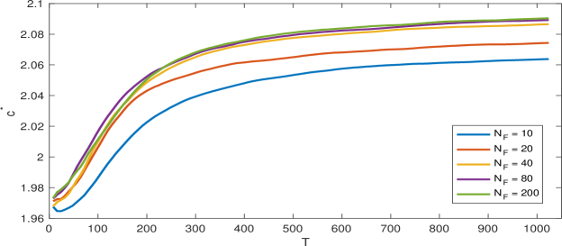
We can see from Figure 2 that in one random realization, as we increase the Fourier modes number, the principal eigenvalues we get are very close when the Fourier modes number $N_{F}$ is near or larger than 200 in this case.

4.2 IPM vs. Semi-Lagrangian computation of KPP front speed

4.2.1 2D cellular flow

We compare interacting particle method, spectral and semi-Lagrangian methods in computing KPP front speeds in 2D cellular flow:

(82) $$v(x,y)=\delta\cdot\big{(}-\sin(x)\cos(y),\ \cos(x)\sin(y)\big{)}.$$

We take the spectral method as a benchmark and select $\delta$ from $2^{0}$ to $2^{4}$. Figure 3(a) shows that these three methods give similar results. The log-log fitted curve has a slope of 0.257 so that $c^{*}=O(\delta^{0.257})\approx O(\delta^{0.25})$, consistent with theory [25]. In Figure 3(a) semi-Lagrangian and spectral methods are in agreement. Figure 3(b) is an example for searching $\lambda\bm{e}$ to reach minimal front speed. Here $\bm{z}=(1,0)$. We do a grid search for the optimal vector $\lambda\bm{e}$ and determine $c^{*}(\bm{z})$ by its variational formula. We found that the optimal dual direction vector $\bm{e}$ is either equal to $\bm{z}$ or near $\bm{z}$. The former occurs for randomly perturbed flows and reduces the search to only the scalar variable $\lambda$ thereby saving computation time. The latter occurs for flows with ordered streamlines (e.g. cellular flows) for which a local search around $\bm{z}$ suffices instead of a time-consuming global research.

(a) Comparison of $c^{*}$ in 2D Cellular flow

(b) Search for $\lambda\bm{e}$, $\delta=2^{2}$

Figure 3: Computation of $c^{*}$ in 2D Cellular flow

4.2.2 2D random shear flow

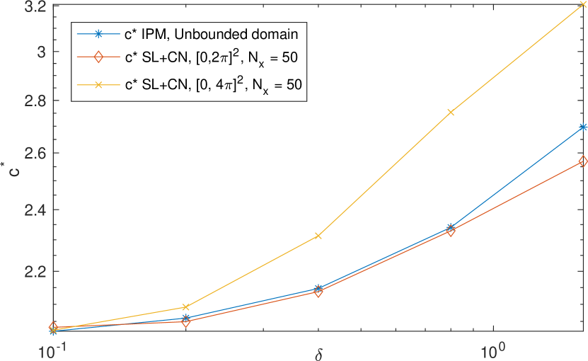
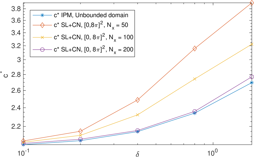
Now we adjust the velocity field with only generated random shear field, i.e. $v(x,y)=\delta\cdot(0,\xi(x))$. Here we would like to simulate the case with an unbounded domain setting. And we can see that given sufficient monte carlo number $N$ and evolution time $n$ in the IPM method, the Semi-Lagrangian method needs increasingly fine grids to get similar results. And during the process that we enlarge the domain to ’infinity’, for the IPM method, we just need to change the initial distribution and similarly compute the particle traces. This does not have any effect on the computation time. For the Semi-Lagrangian method, as we enlarge the domain, we will need to increase the same number of times of the grids if we want to maintain the same partition accuracy. We compute the KPP front speed $c^{*}$ in different domain settings by these two methods with the same random realization. As in [23], for the advection-reaction step, we use a semi-Lagrangian scheme; and for the diffusion step, we use an implicit Crank-Nicholson scheme in time and spectral method in space. We denote this method as SL+CN. In the SL+CN method, if we would like to simulate the situation with an unbounded domain, we can only enlarge the domain step by step. For example, we start with the domain $\mathbb{T}^{2}=[0,2\pi]^{2}$ and enlarge it to $[0,4\pi]^{2},\ [0,8\pi]^{2},\ ...\$. In the Eulerian framework of the SL+CN method, we need to divide the whole domain into $N_{x}\times N_{y}$ grids. Here for simplicity, we just assume $N_{x}=N_{y}$ and if we want to maintain the mesh size during the process of enlarging the domain, the time cost will get more and more expensive. If we would like to maintain the time cost, then the accuracy of the SL+CN method will get worse and worse. The time complexity of the Semi-Lagrangian method is proportional to the number of grid points, i.e. if we set domain length as $L$ and maintain the mesh size, then the advection-reaction step’s time complexity is $O(N_{x}^{2})=O(L^{2})$ in 2D cases. Benefiting from the FFT algorithm, the time complexity of the diffusion step is $O(L\log L)$. Time cost will become more expensive when we consider 3D cases by SL+CN.

(a) Same $N_{x}$, different domain length

(b) Same domain length, different $N_{x}$

Figure 4: Comparison of $c^{*}$ by IPM and SL+CN method

It is seen from Figure 4(a) and 4(b) that as the domain size $L$ gets larger, more grid points are needed to maintain the accuracy of SL+CN method.

4.3 IPM computation of KPP front speeds in random flows

4.3.1 Randomly perturbed 2D cellular flow

Here we change the velocity field into 2D cellular flow with random perturbation. The approximation to the random perturbation is generated by the random Fourier method, i.e. the velocity field is now changed into:

(83) $$v(x,y)=\delta\cdot(-\sin(x)\cos(y),\ \cos(x)\sin(y)+\epsilon\cdot\xi(x)).$$

Here $\xi(x)$ is defined the same as (81) and follows the same energy spectral density $E(k)$ defined in (80). This is a 2D cellular flow with a random perturbation. In this numerical experiment, we set the domain $\mathcal{D}=\mathbb{T}^{2}$ and the iteration number $n=256,\ \Delta t=2^{-9}$, monte carlo number $N=100,000$ (sufficient large). For the random velocity field, we set $N_{F}=400$, $\Delta k=\frac{1}{20\pi}$, $k_{j}=j\Delta k$, $\Delta k_{0}=\frac{1}{2}\Delta k$ and $\Delta k_{j}=\Delta k\ (j>0)$. Then we compute the KPP front speeds with different coefficients of the random perturbation.

Figure 5: Log-log plot of $c^{*}$-$\delta$ in 2D random cellular flow with different $\epsilon$, $z=(1,0)$

Figure 6: Log-log plot of $c^{*}$-$\delta$ in 2D random cellular flow with different $\epsilon$ and $z$

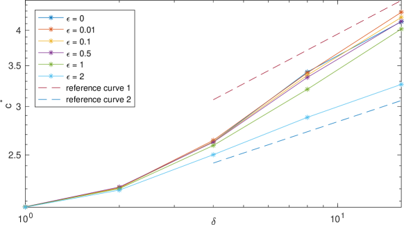
In Figure 5, the two reference curves are with slopes of 0.26 and 0.17. Here we compute 30 realizations and take their averages. During the computation process, we found that the variance of these different realization samples is very small. Then from Figure 5, we can see that: (1) As the coefficient of the random term $\epsilon$ is not equal to zero and increases, the front speed with direction $\bm{z}=(1,0)$, This term demonstrate the power-law scaling of $c^{*}$ concerning $\delta$, the fitted curves’ slope is getting smaller and smaller. (2) As the coefficient of the random term $\epsilon$ decreasing and converging to zero, the front speed $c^{*}$ converges to the case with no random term (i.e. $\epsilon=0$).

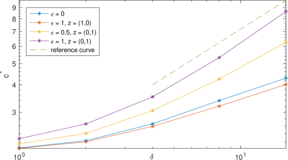
Then we changed the direction $\bm{z}=(0,1)$ and remain other parameters the same and get Figure 6. In Figure 6, the reference curve’s slope is 0.64. We can see that if we change the direction $\bm{z}$ into $(0,1)$, then as the random coefficient $\epsilon$ increases, the front speed $c^{*}$ will also increase.

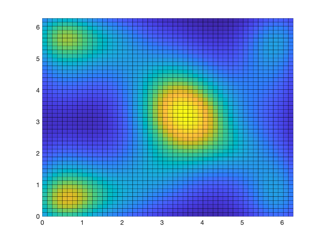
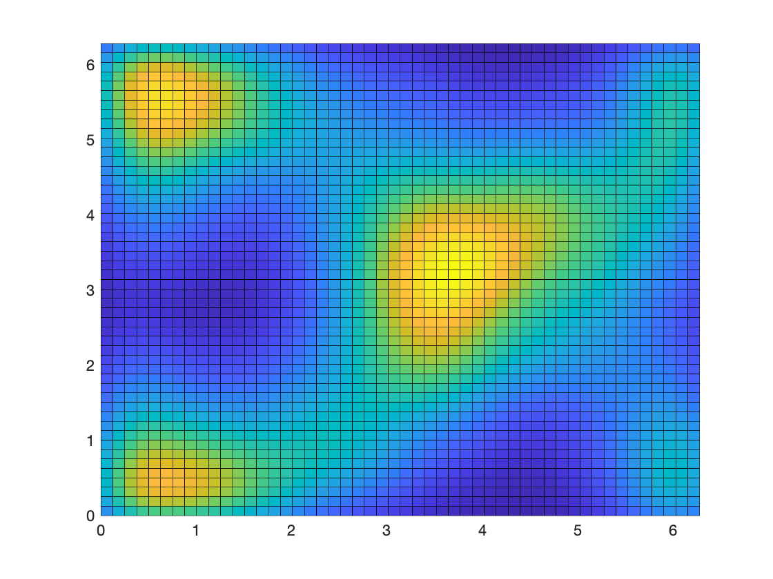
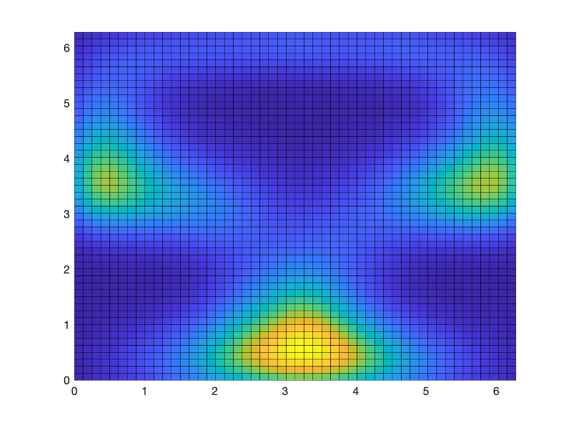
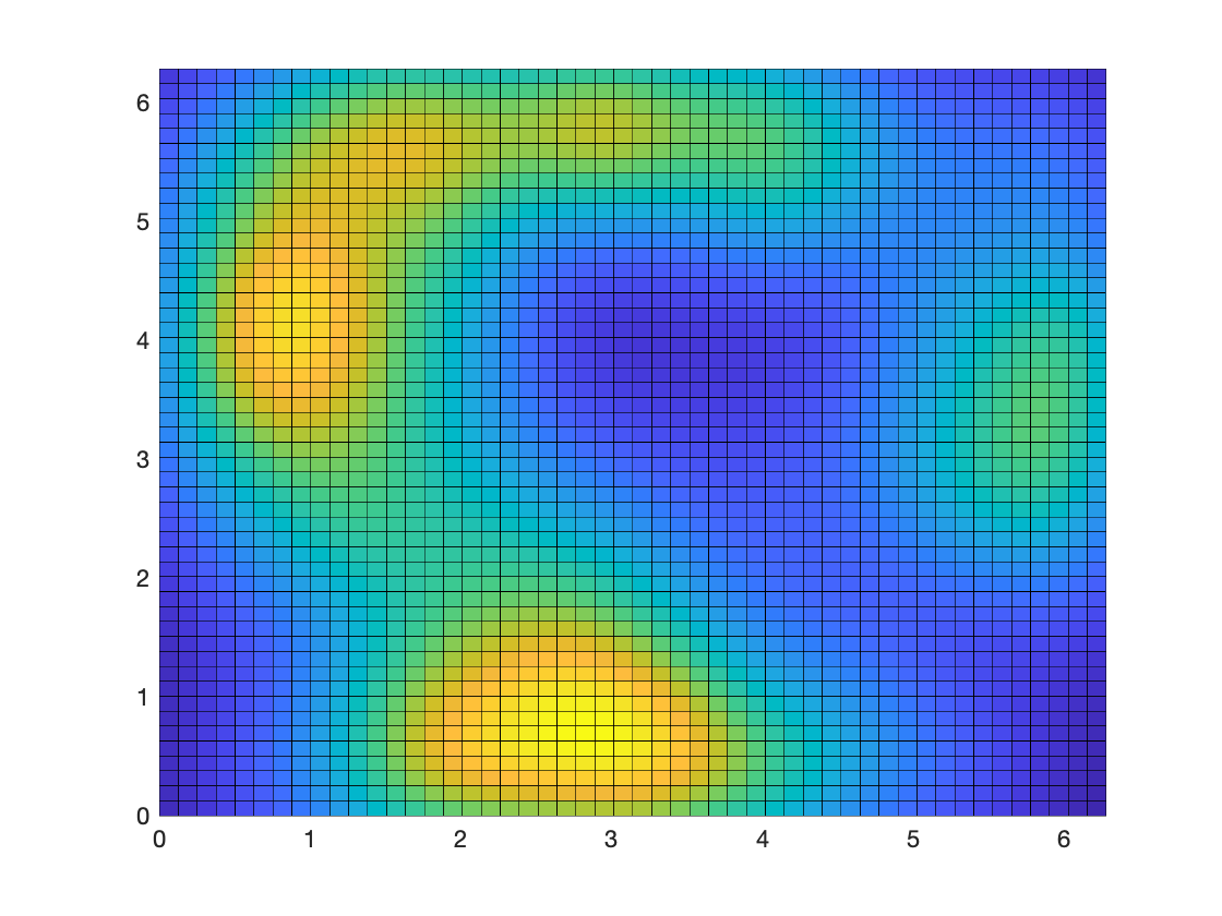
Then we compare the invariant measure of 2D Cellular flow with and without the addition of random perturbation term on domain $\mathbb{T}^{2}$. From Figure 7, by comparing with the sub-figures without random term (Left: 7(a) and 7(c)) and the invariant measure of the sub-figures with the random term (Right: 7(b) and 7(d)), we can see that the addition of the random term creates a degree of disruption to original invariant measure.

(a) $\epsilon=0,\ z=(1,0)$

(b) $\epsilon=1,\ z=(1,0)$

(c) $\epsilon=0,\ z=(0,1)$

(d) $\epsilon=0.5,\ z=(0,1)$

Figure 7: Comparison of invariant measure in 2D (random) Cellular flow

4.3.2 2D random shear flow

In this part, we changed the velocity field into the generated random shear flow, i.e.

(84) $$\bm{v}=v(x,y)=\delta\cdot(0,\ \xi(x)).$$

With this random shear velocity field flow setting, we consider about the front speed $c^{*}$ with direction $\bm{z}=(0,1)$. After searching for the direction $\bm{e}$, we found that $\bm{e}=(1,0)$ can reach the front speeds. For $\bm{e}=(1,0)$, we can analyze this case from the system

(85) $$q_{t}=\mathcal{A}q:=\kappa\Delta_{\bm{x}}q+(-2\kappa\lambda\bm{e}+\bm{v})\cdot\nabla_{\bm{x}}q+(\kappa\lambda^{2}-\lambda\bm{v}\cdot\bm{e}+f^{\prime}(0))q.$$

Decompose the operator $\mathcal{A}$ into $\mathcal{A=L+C}$ where,

(86) $$\mathcal{L}:=\kappa\Delta_{\bm{x}}+(-2\kappa\lambda\bm{e}+\bm{v})\cdot\nabla_{\bm{x}}\ \text{and}\ \mathcal{C}:=(\kappa\lambda^{2}-\lambda\bm{v}\cdot\bm{e}+f^{\prime}(0)).$$

When $\bm{e}=(1,0)$, we can see that $\bm{v}\cdot\bm{e}=0$, the potential is always a constant. Only has a shift effect on particles and reflects on the front speed $c^{*}$. So no matter how we change the amplitude of the velocity field $\delta$, the front speed $c^{*}$ will always remain at a constant.

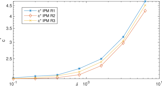
So here we only consider the front speed $c^{*}$ with $\bm{z}=(0,1)$ in this random shear flow setting. Additionally, at this time we do not limit the domain $\mathcal{D}=\mathbb{T}^{2}$, but enlarging it into infinity (with an unbounded domain setting). In the following experiments with unbounded domain setting, we initialize the particles with uniform distribution on $\mathbb{T}^{2}$. Then the particles can spread among unbounded domains and we give them sufficient time to move and spread out. By realizing the random shear velocity field with different random seeds, we compute the KPP front speeds $c^{*}$, and the results are shown in Figure 8.

Figure 8: Log-log plot of $c^{*}$ - $\delta$ , $z=(0,1)$, 2D random shear flow, IPM

4.3.3 Randomly perturbed ABC flow

Here we change the velocity field into 3D ABC flow with random perturbation, i.e. the velocity field is changed into

(87) $$v(x,y,z)=\delta\cdot\big{(}\sin(z)+\cos(y),\ \sin(x)+\cos(z)+\epsilon\cdot\xi(x),\ \sin(y)+\cos(x)\big{)}.$$

And here we set $n=512,\ \Delta t=2^{-11}$, $N=100,000$ and $\epsilon=0$ firstly. Then we compute the front speed $c^{*}$ with three realizations and take their average.

Figure 9: Log-log plot of $c^{*}$ - $\delta$ , $\epsilon=0,z=(0,1,0)$, 3D ABC flow

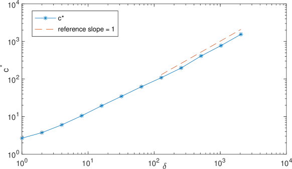
From Figure 9 we can see the result that the fitted curve’s slope in log scale at relative large $\delta$ is 0.9842, i.e. $c^{*}=O(\delta^{0.9842})\approx O(\delta^{1})$. This means the fitted curve’s slope is close to the reference curve with slope $=1$ in log scale at relatively large $\delta$. This result is consistent with the result in [29].

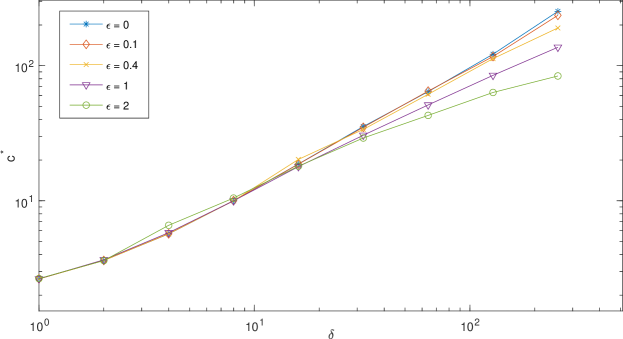
Now if we change the random coefficient $\epsilon$ to make it not equal to 0 and compute the front speed $c^{*}$ corresponding to these cases. Then we will find in Figure 10 that, with the addition of random term and increasing its amplitude, $c^{*}$ in 3D ABC flow will get smaller and smaller. This is because the random term gradually destroys the principal vortex structure [3] (ballistic orbits, [37, 9, 18]) in the ABC flow.

Figure 10: Log-log plot of $c^{*}$ - $\delta$ with different $\epsilon$, 3D randomly perturbed ABC flow

4.3.4 Randomly perturbed 3D cellular flow

Here we consider the 3D cellular flow with random perturbation, the velocity field is changed into $v(x,y,z)=$

(88) $$\delta\cdot\big{(}-\sin(x)\cos(y)\cos(z),\ -\sin(y)\cos(x)\cos(z)+\epsilon\cdot\xi(x),\ 2\sin(z)\cos(x)\cos(y)\big{)}.$$

Here we set $n=512,\ \Delta t=2^{-11}$, $N=100,000,\ \epsilon=0,0.1,0.4,1,2$ and compute their corresponding $c^{*}$.

Figure 11: Log-log plot of $c^{*}$ - $\delta$ with different $\epsilon$, 3D randomly perturbed cellular flow

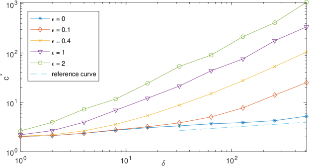
In Figure 11, the reference curve has a slope of 0.13. We can see that when $\epsilon=0$, the fitted curve has the slope 0.1351 and this result is consistent with the result in [29]. As the random perturbation strengthens by tuning up $\epsilon$, the corresponding slopes of the fitted curves and $c^{*}$ values are getting larger. The addition of the random perturbation term destroys the closed streamline structures in 3D cellular flow (reduces trapping) and enhances particle transport thereby $c^{*}$ increases.

4.4 IPM with dynamic shift for particles on unbounded domain

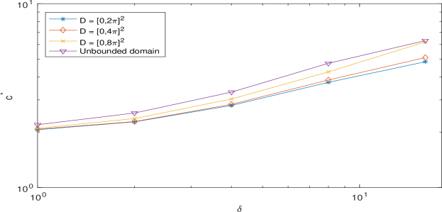
By removing the boundary restriction step in Algorithm 1, IPM can be readily implemented for computing $c^{*}$ on unbounded domains. In order to investigate whether the $c^{*}$ computed by IPM with gradually increasing domain sizes will converge to unbounded domain results, we conduct experiments on the randomly perturbed 2D cellular flow(83). Fig. 12 shows that as the domain size becomes larger, the $c^{*}$ computed with the same random realization converges to the direct result on unbounded domain.

Figure 12: Log-log $c^{*}$-$\delta$ with increasing domain sizes, $\epsilon=0.5$, 2D random cellular flow.

In the convergence analysis of section 3, we require a bounded domain (e.g. $\mathbb{T}^{d}$) to guarantee the existence of the principal eigenvalue and carry out the subsequent $c^{*}$ error analysis. In a future theoretical analysis on unbounded domains, we will work with the Lyapunov exponent as a limit of principal eigenvalue in the infinite volume limit of $\mathbb{T}^{d}$ (as $\text{vol}\,(\mathbb{T})\uparrow\infty$) similar to the periodization approach to stochastic homogenization [11, 7] . Our IPM can be adapted (dropping domain restriction in step 4) to compute particle distribution on unbounded domains ($\mathbb{R}^{d}$) directly. Different from the $\mathbb{T}^{d}$ case, the convergence to an invariant measure requires a dynamic shift to remove a mean flow induced drift.

The SDE system (7), due to $\bm{b}=-2\kappa\lambda\bm{e}+\bm{v}$ and $\bm{v}$ being mean zero, has a nonzero mean drift $-2\kappa\lambda\bm{e}$. If we do not have particle motion limited on a bounded domain, the particles spread due to nonzero mean drift and do not converge to an invariant measure at large times. To make sense of convergence, we introduce a dynamic shift to center the particle ensemble over $j$ generations (each of duration $T$). At each $j$, we shift all particles in the ensemble by $2j\kappa\lambda T$. Due to the stationarity of the random flows, the statistics of the particle evolution are invariant. After the principal eigenvalue approximations have converged, we post-process and map the particle ensemble back to a bounded domain $\mathcal{D}$ for visualization. For example $\mathcal{D}=\mathbb{T}^{d}$, then map with function $mod(\cdot)$, the multi-dimensional modulo operation. To summarize, the particle distribution at the output of the dynamically shifted IPM without domain restriction on $\mathbb{R}^{d}$ converges to an invariant measure subject to deterministic mapping.

4.4.1 2D random shear flow

(89) $$\bm{v}=v(x,y)=\delta\cdot(0,\ \xi(x)).$$

We analyze IPM performance in the two cases: $\bm{e}=(1,0)$ and $\bm{e}=(0,1)$. When $\bm{e}=(0,1)$, $\bm{v}\cdot\bm{e}=\delta\cdot\xi(x)$, the eigen-function only depends on $x$. In operator $\mathcal{L}$, $(-2\kappa\lambda\bm{e}+\bm{v})=(0,\ \delta\cdot\xi(x)-2\kappa\lambda)$ and $\nabla_{\bm{x}}=(\cdot,0)$. The inner product of the two terms is zero. This operator is then a 1D random Schrodinger operator in $x$ with well-known localization property. And when $\bm{e}=(1,0)$, $\bm{v}\cdot\bm{e}=0$, the potential is always a constant, adding a translation on particle. To see what is the effect of adding space random perturbation term on the 2D cellular flow, we investigate how the invariant measure (particle distribution) changes after we dynamically shift them. Here we set $\delta=2^{2}$, $N=200,000$, and other parameters remain the same.

Figure 13: Particles distribution under dynamic shift, $t=8$ to $t=64$, $e=(1,0)$

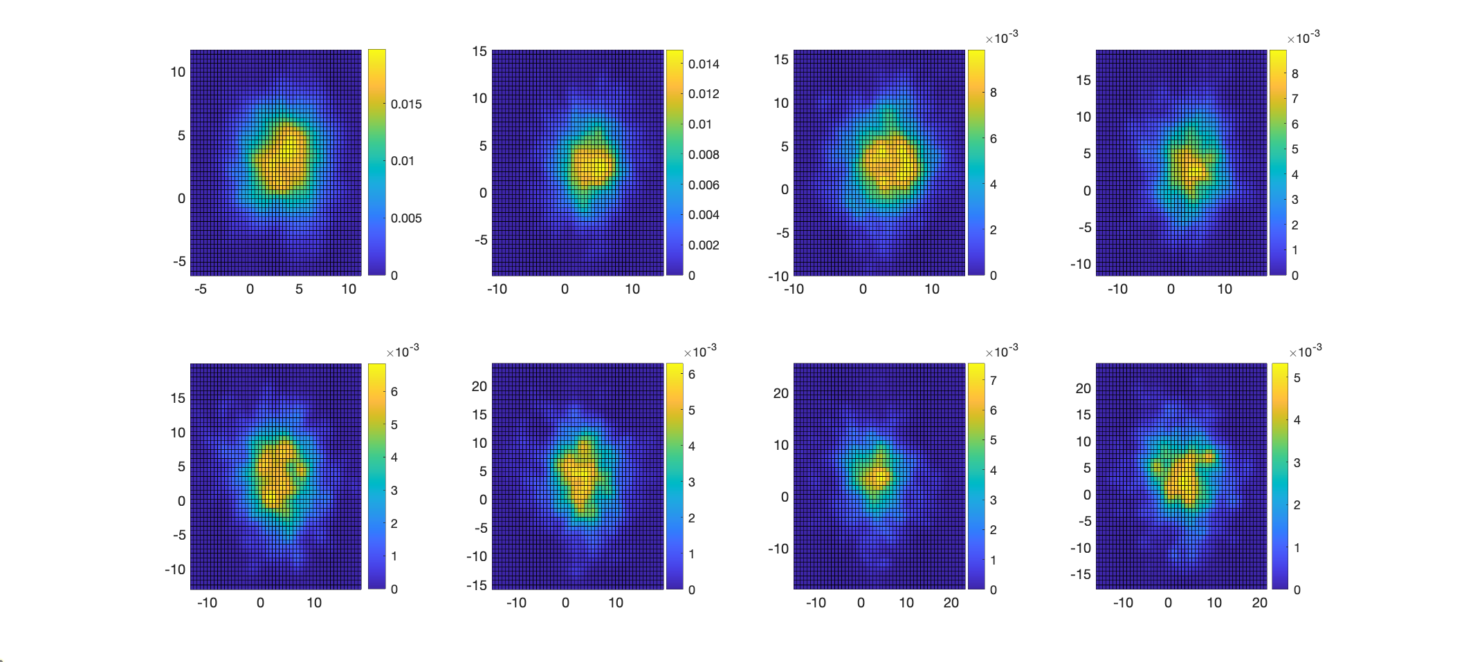
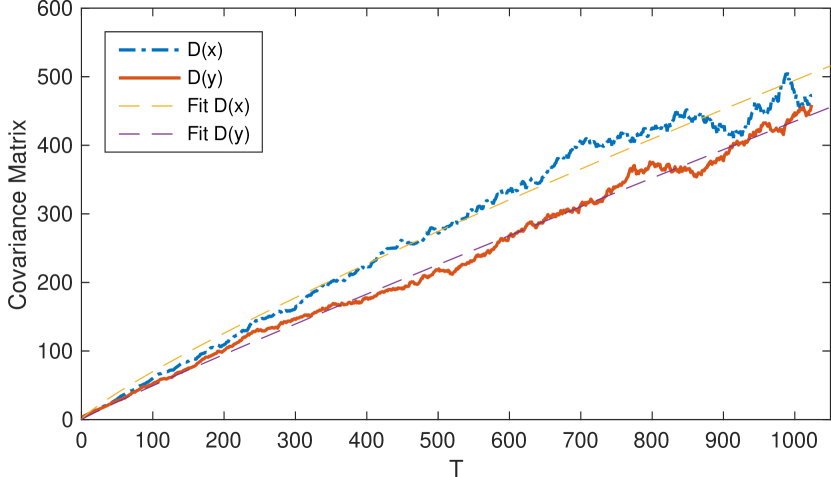
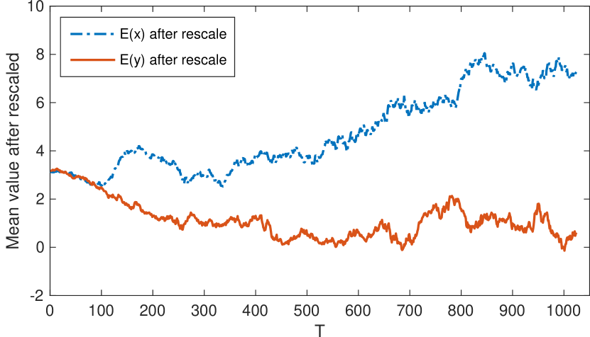
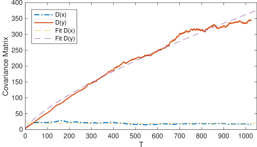
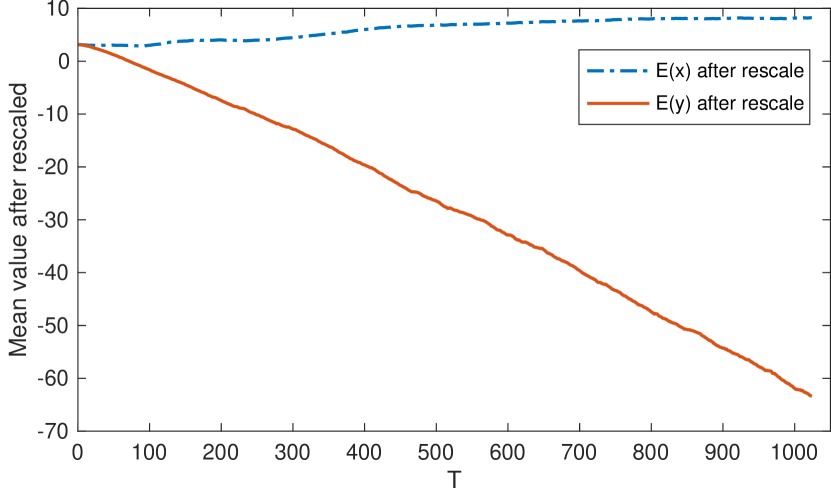
Here we can see from Figure 13 that, at the early stage of the experiment, the particles are continually spreading outwards from the initial area. A similar case occurs with $\bm{e}=(0,1)$. For the performance of the particle distribution at long times, we use the re-scaled center $E(\cdot)$ and the second-order momentum $D(\cdot)$ of the particles to express them. We take their average value over ten realizations. In Figure 14(a), the order of the diffusion in direction $x$ and in direction $y$ are respectively $D(x)=O(t^{0.850})$ and $D(y)=O(t^{0.945})$. In Figure 15(a), the order of the diffusion in direction $x$ and in direction $y$ are respectively $D(x)=O(t^{-0.013})\approx O(t^{0})$ and $D(y)=O(t^{0.742})$. We also perform common statistical tests of the particle distribution at $t=1024$ (e.g. QQplot and KS test), and the results all show that the particle distribution is non-Gaussian. In fact, according to the variation of the variance $D(x),D(y)$ with time $t$, it can be seen that the diffusion of the particles after the re-center process exhibits sub-diffusion phenomena.

(a) Covariance matrix

(b) Mean value

Figure 14: Covariance matrix and mean value evolution, $t=0$ to $t=1024$, $e=(1,0)$

(a) Covariance matrix

(b) Mean value

Figure 15: Covariance matrix and mean value evolution, $t=0$ to $t=1024$, $e=(0,1)$

(a) qqplot in $x$, $e=(1,0)$

(b) histogram in $x$, $e=(1,0)$

Figure 16: QQ plot and histogram plot for random shear flow, $\bm{e}=(1,0),t=1024$

4.4.2 3D randomly perturbed ABC flow

(90) $$v(x,y,z)=\delta\cdot\big{(}\sin(z)+\cos(y),\ \sin(x)+\cos(z)+\epsilon\cdot\xi(x),\ \sin(y)+\cos(x)\big{)}.$$

Here we plot the distribution of the particles with different random coefficients in $\mathbb{T}^{3}$. It can be shown from Figure 17, especially the $xz$-plane that as the coefficient of the random term gradually increases, the radius of the exhibited tube structure becomes larger and larger with the same total number of particles, which means that the distribution of particles becomes more and more dispersed and the tube structure is more and more severely damaged. A similar case also occurs if we change the system with an unbounded domain setting and at the final plot step we restrict the distribution of the particles on $\mathbb{T}^{3}$.

(a) $\epsilon=0$

(b) $\epsilon=0.4$

(c) $\epsilon=2$

Figure 17: Three planar views of particle distributions for randomly perturbed ABC flow at $\epsilon=0,0.2,0.4$, showing increased blurring/broadening effect of perturbations.

5 Conclusions

We developed an efficient interacting particle method (IPM) to compute KPP front speeds $c^{*}$ in 2D and 3D stochastic flows, with convergence analysis based on the random Fourier method. We first computed $c^{*}$ in periodic flows, including 2D cellular flow and 3D Arnold-Beltrami-Childress (ABC) flow, to reach agreement with semi-Lagrangian and spectral methods. Then we computed and analyzed the effect of random perturbations on $c^{*}$. As the perturbation strengths increase, we observed that the vortical structures (ballistic orbits) [3, 37, 18, 9] in 3D ABC flow are collapsing, resulting in smaller $c^{*}$. Compared with mesh based methods, IPM has several striking advantages: (1) it is scalable in spatial dimension and can handle stochastic 3D problems at ease; (2) it is scalable in domain size and can handle infinite domain as well as Lyapunov exponent approximation directly. In experiments on $\mathbb{R}^{3}$, the empirical particle distributions from IPM show convergence under dynamic normalization while the average particle fitness approximates the Lyapunov exponent.

Appendix A Convergence of perturbed $\mu$

We review perturbation theory of linear operators with the following notation:

(91) $$T(a)=T+a\cdot T^{\prime}.$$

Here $T$ is the original operator, $T^{\prime}$ is the perturbation operator and $a$ is the coefficient of the perturbation term. Then we have the following property

Proposition 1.

Let $T(a)$ be continuous at $a=0$, then the eigenvalues of $T(a)$ are continuous at $a=0$. If $\lambda$ is an eigenvalue of $T(0)=T$, then the $\lambda$-group is well-defined for sufficiently small $|a|$ and the total projection $P(a)$ for the $\lambda$-group is continuous at $a=0$.

Next, we would like to introduce some notations we use to describe the convergence between operators in the generalized sense.

Definition 2.

Consider closed linear manifolds $M$ and $N$ of a Banach space $Z$. We use $S_{M}$ to denote the unit sphere of $M$ (the set of all $v\in M$ which satisfy $||v||=1$). For any two closed linear manifolds $M,N$ of $Z$, we define

(92) $$\delta(M,N)=\sup_{u\in S_{M}}dist(u,M),$$

(93) $$\tilde{\delta}(M,N)=\max[\delta(M,N),\delta(N,M)]^{1}.$$

Definition 3.

We denote that $T_{n}$ converge to $T$ in the generalized sense if $\tilde{\delta}(T_{n},T)\to 0$.

There is a proposition that is a sufficient condition for the generalized convergence and its proof can be found in [10].

Proposition 4.

Let $T\in\mathcal{C}(X,Y)$. Let $A_{n},n=0,1,2,\cdots$, be $T$-bounded so that $||A_{n}v||\leq a_{n}||v||+b_{n}||Tv||$ for $v\in D(T)\subset D(A_{n})$. If $a_{n}\to 0$ and $b_{n}\to 0$, then $T_{n}=T+A_{n}\in\mathcal{C}(X,Y)$ for sufficiently large $n$ and $T_{n}\to T$ in the generalized sense.

Next, we would like to review some results which can make the above propositions applicable to an infinite system. Here we use $\Sigma(T)$ to denote the spectrum of the operator $T\in\mathcal{C}(X)$ and we suppose that the spectrum $\Sigma(T)$ has an isolated point $\lambda$. Then obviously we can divide $\Sigma(T)$ into two parts $\Sigma^{\prime}(T)$ and $\Sigma^{\prime\prime}(T)$. Here $\Sigma^{\prime}(T)$ consists of the single point $\lambda$ and any simple closed curve $\Gamma$ enclosing $\lambda$ but no other point in $\Sigma(T)$ may be chosen. Following this idea, we can divide the spectrum of an infinity system and focus on the finite system $\Sigma^{\prime}(T)$ which contains the principal eigenvalue and we have the following proposition to analyze the continuity of a finite system of eigenvalues.

Proposition 5.

The change of a finite system $\Sigma^{\prime}(T)$ of eigenvalues of a closed operator $T$ is small (in the sense of 1) when $T$ is subjected to a small perturbation in the sense of generalized convergence.

Appendix B Computing upper bounds in the assumptions

From the random Fourier method mentioned in Section 2.2, the approximated velocity field $\bm{v}_{F}$ generated by (17) will follow a correlation function $R_{F}$ defined in (19). And the true random velocity field $\bm{v}_{r}$ will follow the correlation function $R$ defined in (18). In the above convergence analysis in [15], the author assumed that the deterministic $\bm{b}_{0}(\bm{x})$ and $c_{0}(\bm{x})$ satisfy that $||\bm{b}_{0}(\bm{x})||\leq M_{1}$, $|c_{0}(\bm{x})|\leq M_{2}$, $||\nabla_{\bm{x}}c_{0}(\bm{x})||\leq M_{3}$ and $||\Delta_{\bm{x}}c_{0}(\bm{x})||\leq M_{4}$.Now we analyze these assumptions with the addition of random perturbation $\bm{v}_{r}$ and we use $\bm{v}_{F}$ to be an approximation to $\bm{v}_{r}$ in the practical experiments. By the triangle inequality, we can get that

(94) $$||\bm{b}(\bm{x},\omega)||_{L^{2}}\leq||\bm{b}_{0}(\bm{x})||_{L^{2}}+||\bm{v}_{r}(\bm{x},\omega)||_{L^{2}}\leq M_{1}+||\bm{v}_{r}(\bm{x},\omega)||_{L^{2}}.$$

Here we give the analysis for 2D cases as an example, a similar analysis can be done for higher dimensions. Here $\bm{x}=(x,y)$ and due to $\bm{v}_{r}$ is a 1D random perturbation, then we have $\bm{v}_{r}(\bm{x},\omega)=(0,v_{r}(x,\omega))$. We assume that $v_{r}(x,\omega)\in L^{1}(\mathbb{R})\cap L^{2}(\mathbb{R})$ almost surely. We also denote the period for the deterministic part is $L$ and choose $\mathcal{D}=[0,L]^{2}$. Then for the term $||\bm{v}_{r}(\bm{x},\omega)||_{L^{2}}$, we can analyze it on $\mathbb{R}^{1}\times[0,L]$ and obtain

(95) $$\mathbb{E}_{\omega}[||\bm{v}_{r}(\bm{x},\omega)||_{L^{2}}^{2}]\leq\mathbb{E}_{\omega}[\int_{0}^{L}\int_{-\infty}^{+\infty}|v_{r}(x,\omega)|^{2}dxdy]=L\cdot\mathbb{E}_{\omega}[\int_{-\infty}^{+\infty}|v_{r}(x,\omega)|^{2}dx].$$

We denote $\widehat{v_{r}}(k,\omega):=\mathcal{F}[v_{r}](k)$, the Fourier transform of $v_{r}(x,\omega)$. From the definition of energy spectral density, we know that $E(k)=\mathbb{E}_{\omega}[|\widehat{v_{r}}(k,\omega)|^{2}]$. Then by Plancherel theorem, we can get the following relationship.

(96) $$L\cdot\mathbb{E}_{\omega}[\int_{-\infty}^{+\infty}|v_{r}(x,\omega)|^{2}dx]=L\int_{-\infty}^{+\infty}\mathbb{E}_{\omega}[|\widehat{v_{r}}(k,\omega)|^{2}]dk=L\int_{-\infty}^{+\infty}E(k)dk=R(0)L.$$

Then we can get $\mathbb{E}_{\omega}[||\bm{b}(\bm{x},\omega)||_{L^{2}}]\leq M_{1}+\sqrt{R(0)L}$. And we know the variance $Var(||\bm{b}(\bm{x},\omega)||_{L^{2}})$ $\leq\mathbb{E}_{\omega}[||\bm{v}_{r}||_{L^{2}}^{2}]\leq R(0)L$. Then for a probability $p$ close to 1, we can find the corresponding upper bound $M_{1,r}$, so that $P(||\bm{b}(\bm{x},\omega)||_{L^{2}}<M_{1,r})>p$. For $\bm{v}_{F}$, it will have a period $1/\Delta k$ in dimension $x$, then we can give the analysis for $\bm{v}_{F}$ on $[0,\text{lcm}(L,1/\Delta k)]\times[0,L]$. Then similar analysis can be done for $||\bm{b}^{\prime}(\bm{x},\omega)||_{L^{2}}=||\bm{b}_{0}(\bm{x})+\bm{v}_{F}||_{L^{2}}$ and we can get an upper bound $M_{1}^{\prime}$. Then we take $M_{1}^{*}=\max(M_{1,r},$ $M_{1}^{\prime})$. Then for the second assumption, we have

(97) $$|c(\bm{x},\omega)|=|c_{0}(\bm{x})-\lambda\bm{v}_{r}(\bm{x},\omega)\cdot\bm{e}|\leq|c_{0}(\bm{x})|+\lambda\cdot||\bm{v}_{r}(\bm{x},\omega)||_{L^{2}}\leq M_{2}+\lambda\cdot||\bm{v}_{r}(\bm{x},\omega)||_{L^{2}}.$$

Then we can get $\mathbb{E}_{\omega}[|c(\bm{x},\omega)|]\leq M_{2}+\sqrt{\sqrt{\pi}L}$. And we know the variance $Var(|c(\bm{x},\omega)|)\leq\mathbb{E}_{\omega}[||\bm{v}_{r}||_{L^{2}}^{2}]\leq\sqrt{\pi}L$. Then for a probability $p$ close to 1, we can find the corresponding upper bound $M_{2,r}$, so that $P(|c(\bm{x},\omega)|<M_{2,r})>p$. Similar analysis can be done for $|c^{\prime}(\bm{x},\omega)|$ and we can get an upper bound $M_{2}^{\prime}$. Then we take $M_{2}^{*}=\max(M_{2,r},M_{2}^{\prime})$. Then for the third and fourth assumptions, we have

(98) $$||\nabla_{\bm{x}}c(\bm{x},\omega)||_{L^{2}}\leq||\nabla_{\bm{x}}c_{0}(\bm{x})||_{L^{2}}+\lambda\cdot||\nabla_{\bm{x}}\bm{v}_{r}(\bm{x},\omega)||_{L^{2}}\leq M_{3}+\lambda\cdot||\nabla_{\bm{x}}\bm{v}_{r}(\bm{x},\omega)||_{L^{2}},$$

(99) $$||\Delta_{\bm{x}}c(\bm{x},\omega)||_{L^{2}}\leq||\Delta_{\bm{x}}c_{0}(\bm{x})||_{L^{2}}+\lambda\cdot||\Delta_{\bm{x}}\bm{v}_{r}(\bm{x},\omega)||_{L^{2}}\leq M_{4}+\lambda\cdot||\Delta_{\bm{x}}\bm{v}_{r}(\bm{x},\omega)||_{L^{2}}.$$

Then for the term $||\nabla_{\bm{x}}\bm{v}_{r}(\bm{x},\omega)||_{L^{2}}$ and $||\Delta_{\bm{x}}\bm{v}_{r}(\bm{x},\omega)||_{L^{2}}$ , we have

(100) $$||\nabla_{\bm{x}}\bm{v}_{r}(\bm{x},\omega)||_{L^{2}}^{2}\leq\int_{0}^{L}\int_{-\infty}^{+\infty}|\frac{d}{dx}v_{r}(x,\omega)|^{2}dxdy=L\cdot\int_{-\infty}^{\infty}|\frac{d}{dx}v_{r}(x,\omega)|^{2}dx,$$

(101) $$||\Delta_{\bm{x}}\bm{v}_{r}(\bm{x},\omega)||_{L^{2}}^{2}\leq\int_{0}^{L}\int_{-\infty}^{\infty}|\frac{d^{2}}{dx^{2}}v_{r}(x,\omega)|^{2}dxdy=L\cdot\int_{-\infty}^{\infty}|\frac{d^{2}}{dx^{2}}v_{r}(x,\omega)|^{2}dx.$$

By the properties of the Fourier transform and the Plancherel theorem, we can obtain that

$$\mathbb{E}_{\omega}[||\nabla_{\bm{x}}\bm{v}_{r}(\bm{x},\omega)||_{L^{2}}^{2}]\leq L\mathbb{E}_{\omega}[\int_{-\infty}^{\infty}|\frac{d}{dx}v_{r}(x,\omega)|^{2}dx] =L\int_{-\infty}^{\infty}\mathbb{E}_{\omega}[|k\widehat{v_{r}}(k)|^{2}]dk$$

(102) $$=L\int_{-\infty}^{\infty}k^{2}E(k)dk<\infty,$$

$$\mathbb{E}_{\omega}[||\Delta_{\bm{x}}\bm{v}_{r}(\bm{x},\omega)||_{L^{2}}^{2}]\leq L\mathbb{E}_{\omega}[\int_{-\infty}^{\infty}|\frac{d^{2}}{dx^{2}}v_{r}(x,\omega)|^{2}dx] =L\int_{-\infty}^{\infty}\mathbb{E}_{\omega}[|k^{2}\widehat{v_{r}}(k)|^{2}]dk$$

(103) $$=L\int_{-\infty}^{\infty}k^{4}E(k)dk<\infty.$$

Then we can obtain that

(104) $$\mathbb{E}_{\omega}[||\nabla_{\bm{x}}c(\bm{x},\omega)||_{L^{2}}]\leq M_{3}+L\int_{-\infty}^{\infty}k^{2}E(k)dk$$

(105) $$\mathbb{E}_{\omega}[||\Delta_{\bm{x}}c(\bm{x},\omega)||_{L^{2}}]\leq M_{4}+L\int_{-\infty}^{\infty}k^{4}E(k)dk.$$

And we also know the upper bound of their variance. Following the same idea, we can get $M_{3,r}$ and $M_{4,r}$, the upper bound hold with probability greater than $p$. Following the same idea, we can get $M_{3}^{\prime}$ and $M_{4}^{\prime}$. Then we take $M_{3}^{*}=\max(M_{3,r},M_{3}^{\prime})$ and $M_{4}^{*}=\max(M_{4,r},M_{4}^{\prime})$. We have already computed the assumptions’ upper bound distributions after adding a random perturbation with specific energy spectral density.

Appendix C Proof for Theorem 66

Proof C.1.

By the operators defined in Lemma 3.5, we can get that

(106) $$\mathcal{U}(T,0)-\prod_{h=1}^{H}e^{\Delta t_{h}\mathcal{L}^{\prime}(\bm{x},\omega)}e^{\Delta t_{h}\mathcal{C}^{\prime}(\bm{x},\omega)}=e^{\gamma T}\big{(}\mathcal{U}_{\gamma}(T,0)-\prod_{h=1}^{H}e^{\Delta t_{h}\mathcal{L}_{\gamma}^{\prime}}e^{\Delta t_{h}\mathcal{C}_{\gamma}^{\prime}}\big{)}.$$

By the telescopic sum argument, we obtain that for any $q\in\mathcal{D}$,

$$e_{3}= ||\prod_{h=1}^{H}e^{\Delta t_{h}\mathcal{L}(\bm{x},\omega)}e^{\Delta t_{h}\mathcal{C}(\bm{x},\omega)}q-\prod_{h=1}^{H}e^{\Delta t_{h}\mathcal{L}^{\prime}(\bm{x},\omega)}e^{\Delta t_{h}\mathcal{C}^{\prime}(\bm{x},\omega)}q||_{L^{2}}$$

$$= e^{\gamma T}\big{|}\big{|}\sum_{j=1}^{H}\prod_{h=j+1}^{H}e^{\Delta t_{h}\mathcal{L}_{\gamma}}e^{\Delta t_{h}\mathcal{C}_{\gamma}}(e^{\Delta t_{j}\mathcal{L}_{\gamma}}e^{\Delta t_{j}\mathcal{C}_{\gamma}}-e^{\Delta t_{j}\mathcal{L}_{\gamma}^{\prime}}e^{\Delta t_{j}\mathcal{C}_{\gamma}^{\prime}})\prod_{i=1}^{j-1}e^{\Delta t_{i}\mathcal{L}_{\gamma}^{\prime}}e^{\Delta t_{i}\mathcal{C}_{\gamma}^{\prime}}q\big{|}\big{|}_{L^{2}}$$

(107) $$\leq e^{\gamma T}||\sum_{j=1}^{H}(e^{\Delta t_{j}\mathcal{L}_{\gamma}}e^{\Delta t_{j}\mathcal{C}_{\gamma}}-e^{\Delta t_{j}\mathcal{L}_{\gamma}^{\prime}}e^{\Delta t_{j}\mathcal{C}_{\gamma}^{\prime}})q||_{L^{2}}.$$

To simplify, we denote $\mathcal{L}_{\gamma}=\mathcal{L}_{\gamma}(\bm{x},\omega)=\mathcal{L}(\bm{x},\omega)-\tilde{\gamma}$ and $\mathcal{C}_{\gamma}=\mathcal{C}_{\gamma}(\bm{x},\omega)=\mathcal{C}(\bm{x},\omega)-M_{2}^{*}$. This step is to guarantee that $||e^{\Delta t\mathcal{L}_{\gamma}(\bm{x},\omega)}||_{L^{2}(\mathcal{D})}\leq 1$ and $||e^{\Delta t\mathcal{C}_{\gamma}(\bm{x},\omega)}||_{L^{2}(\mathcal{D})}\leq 1$ are both satisfied with probability greater than $p$. Same for $\mathcal{L}_{\gamma}^{\prime}$ and $\mathcal{C}_{\gamma}^{\prime}$. By expressing the term $e^{\Delta t\mathcal{C}_{\gamma}}$ and $e^{\Delta t\mathcal{C}_{\gamma}^{\prime}}$ into exponential series, we can obtain

(108) $$e^{\Delta t\mathcal{L}_{\gamma}}e^{\Delta t\mathcal{C}_{\gamma}}q=e^{\Delta t\mathcal{L}_{\gamma}}q+(\Delta t)e^{\Delta t\mathcal{L}_{\gamma}}\mathcal{C}_{\gamma}q+r_{1}(\bm{x},\omega)q,$$

(109) $$e^{\Delta t\mathcal{L}_{\gamma}^{\prime}}e^{\Delta t\mathcal{C}_{\gamma}^{\prime}}q=e^{\Delta t\mathcal{L}_{\gamma}^{\prime}}q+(\Delta t)e^{\Delta t\mathcal{L}_{\gamma}^{\prime}}\mathcal{C}_{\gamma}^{\prime}q+r_{1}^{\prime}(\bm{x},\omega)q.$$

Here the residual terms $||r_{1}(\bm{x},\omega)||_{L^{2}(\mathcal{D})}\leq\frac{1}{2}(\Delta t)^{2}||\mathcal{C}_{\gamma}(\bm{x},\omega)||^{2}_{L^{2}(\mathcal{D})},||r_{1}^{\prime}(\bm{x},\omega)||_{L^{2}(\mathcal{D})}$ $\leq\frac{1}{2}(\Delta t)^{2}$ $||\mathcal{C}_{\gamma}^{\prime}(\bm{x},\omega)||^{2}_{L^{2}(\mathcal{D})}$. Then we denote $r_{1}=r_{1}(\bm{x},\omega),\ r_{1}^{\prime}=r_{1}^{\prime}(\bm{x},\omega)$ and let the two equations above subtract

$$LHS =(e^{\Delta t\mathcal{L}_{\gamma}}-e^{\Delta t\mathcal{L}_{\gamma}^{\prime}})q+(\Delta t)e^{\Delta t\mathcal{L}_{\gamma}}\mathcal{C}_{\gamma}q-(\Delta t)e^{\Delta t\mathcal{L}_{\gamma}^{\prime}}\mathcal{C}_{\gamma}^{\prime}q+r_{1}q-r_{1}^{\prime}q$$

(110) $$=(e^{\Delta t\mathcal{L}_{\gamma}}-e^{\Delta t\mathcal{L}_{\gamma}^{\prime}})\big{(}1+\Delta t\mathcal{C}_{\gamma}\big{)}q+(\Delta t)e^{\Delta t\mathcal{L}_{\gamma}^{\prime}}(\mathcal{C}_{\gamma}-\mathcal{C}_{\gamma}^{\prime})q+(r_{1}-r_{1}^{\prime})q.$$

Then we define $\mathcal{G}(\bm{x},\omega)=\mathcal{L}_{\gamma}(\bm{x},\omega)-\mathcal{L}_{\gamma}^{\prime}(\bm{x},\omega)$ and $\mathcal{H}(\bm{x},\omega)=\mathcal{C}_{\gamma}(\bm{x},\omega)-\mathcal{C}_{\gamma}^{\prime}(\bm{x},\omega)$. By the freezing coefficient formula, we obtain

$$e^{\Delta t\mathcal{L}_{\gamma}(\bm{x},\omega)}-e^{\Delta t\mathcal{L}_{\gamma}^{\prime}(\bm{x},\omega)}= e^{\Delta t\mathcal{L}_{\gamma}^{\prime}(\bm{x},\omega)}+\int_{0}^{\Delta t}e^{s\mathcal{L}_{\gamma}^{\prime}(\bm{x},\omega)}\mathcal{G}(\bm{x},\omega)e^{(\Delta t-s)\mathcal{L}_{\gamma}(\bm{x},\omega)}ds$$

(111) $$-e^{\Delta t\mathcal{L}_{\gamma}^{\prime}(\bm{x},\omega)}=\int_{0}^{\Delta t}e^{s\mathcal{L}_{\gamma}^{\prime}(\bm{x},\omega)}\mathcal{G}(\bm{x},\omega)e^{(\Delta t-s)\mathcal{L}_{\gamma}(\bm{x},\omega)}ds$$

We denote $\mathcal{G}=\mathcal{G}(\bm{x},\omega),\ \mathcal{H}=\mathcal{H}(\bm{x},\omega)$. Then we substitute the above equation (111) into (110) and compute its $L^{2}$ norm.

$$||(e^{\Delta t\mathcal{L}_{\gamma}}-e^{\Delta t\mathcal{L}_{\gamma}^{\prime}})\big{(}1+\Delta t\mathcal{C}_{\gamma}\big{)}q+(\Delta t)e^{\Delta t\mathcal{L}_{\gamma}^{\prime}}(\mathcal{C}_{\gamma}-\mathcal{C}_{\gamma}^{\prime})q+(r_{1}-r_{1}^{\prime})q||_{L^{2}}$$

$$\leq\ ||(e^{\Delta t\mathcal{L}_{\gamma}}-e^{\Delta t\mathcal{L}_{\gamma}^{\prime}})\big{(}1+\Delta t\mathcal{C}_{\gamma}\big{)}q||_{L^{2}}+||(\Delta t)e^{\Delta t\mathcal{L}_{\gamma}^{\prime}}\mathcal{H}q||_{L^{2}}+||(r_{1}-r_{1}^{\prime})q||_{L^{2}}$$

$$\leq\ ||(e^{\Delta t\mathcal{L}_{\gamma}}-e^{\Delta t\mathcal{L}_{\gamma}^{\prime}})\big{(}1+\Delta t\mathcal{C}_{\gamma}\big{)}q||_{L^{2}}+(\Delta t)||\mathcal{H}q||_{L^{2}}$$

$$+\frac{1}{2}(\Delta t)^{2}(||\mathcal{C}_{\gamma}||^{2}_{L^{2}(\mathcal{D})}+||\mathcal{C}_{\gamma}^{\prime}||^{2}_{L^{2}(\mathcal{D})})||q||_{L^{2}}$$

$$\leq\ (\Delta t)||\mathcal{G}q||_{L^{2}}+(\Delta t)^{2}||\mathcal{G}\mathcal{C}_{\gamma}q||_{L^{2}}+(\Delta t)||\mathcal{H}q||_{L^{2}}$$

(112) $$+\frac{1}{2}(\Delta t)^{2}(||\mathcal{C}_{\gamma}||^{2}_{L^{2}(\mathcal{D})}+||\mathcal{C}_{\gamma}^{\prime}||^{2}_{L^{2}(\mathcal{D})})||q||_{L^{2}}.$$

Then substitute this result back to (107), and we can get the error estimate

$$e_{3} =||\prod_{h=1}^{H}e^{\Delta t_{h}\mathcal{L}(\bm{x},\omega)}e^{\Delta t_{h}\mathcal{C}(\bm{x},\omega)}q-\prod_{h=1}^{H}e^{\Delta t_{h}\mathcal{L}^{\prime}(\bm{x},\omega)}e^{\Delta t_{h}\mathcal{C}^{\prime}(\bm{x},\omega)}q||_{L^{2}}$$

(113) $$\leq C_{1}(q,\omega)\Delta t+C_{2}(||\mathcal{G}q||_{L^{2}}+||\mathcal{H}q||_{L^{2}}).$$

Here the coefficients $C_{1}(q,\omega)=Te^{\gamma T}\cdot\Big{(}||\mathcal{G}(\bm{x},\omega)\mathcal{C}_{\gamma}(\bm{x},\omega)q||_{L^{2}}+$$\frac{1}{2}(||\mathcal{C}_{\gamma}(\bm{x},\omega)||^{2}_{L^{2}(\mathcal{D})}+||\mathcal{C}_{\gamma}^{\prime}(\bm{x},\omega)||^{2}_{L^{2}(\mathcal{D})})$ $||q||_{L^{2}}\Big{)}$, $C_{2}=Te^{\gamma T}$. Then due to $||\mathcal{C}_{\gamma}^{\prime}(\bm{x},\omega)||^{2}_{L^{2}(\mathcal{D})}$, $||\mathcal{C}_{\gamma}(\bm{x},\omega)||^{2}_{L^{2}(\mathcal{D})}$ $<1$ are both satisfied with probability greater than $p$, we can obtain that $prob(B_{1})>p$, where $B_{1}=$

(114) $$\Big{\{}e_{3}\leq Te^{\gamma T}\cdot\big{(}||\bm{v}-\bm{v}^{\prime}||_{L^{2}}\cdot\big{(}||\nabla_{\bm{x}}q||_{L^{2}}+\lambda||q||_{L^{2}}\big{)}+(\Delta t)\big{(}||\bm{v}-\bm{v}^{\prime}||_{L^{2}}\cdot||\nabla_{\bm{x}}q||_{L^{2}}+||q||_{L^{2}}\big{)}\big{)}\Big{\}}.$$

Appendix D Proof of Theorem 7

Proof D.1.

$$e^{\Delta t\mathcal{L}_{\gamma}^{j}}e^{\Delta t\mathcal{C}_{\gamma}^{j}}- e^{\Delta t\mathcal{L}_{\gamma}}e^{\Delta t\mathcal{C}_{\gamma}}=e^{\Delta t\mathcal{L}_{\gamma}}e^{\Delta t\mathcal{C}_{\gamma}}[e^{-\Delta t\mathcal{C}_{\gamma}}e^{-\Delta t\mathcal{L}_{\gamma}}-e^{-\Delta t\mathcal{C}_{\gamma}^{j}}e^{-\Delta t\mathcal{L}_{\gamma}^{j}}]e^{\Delta t\mathcal{L}_{\gamma}^{j}}e^{\Delta t\mathcal{C}_{\gamma}^{j}}$$

$$= e^{\Delta t\mathcal{L}_{\gamma}}e^{\Delta t\mathcal{C}_{\gamma}}[e^{-\Delta t\mathcal{C}_{\gamma}}e^{-\Delta t\mathcal{L}_{\gamma}}-e^{-\Delta t\mathcal{C}_{\gamma}^{j}}e^{-\Delta t\mathcal{L}_{\gamma}^{j}}]e^{\Delta t\mathcal{L}_{\gamma}}e^{\Delta t\mathcal{C}_{\gamma}}\ +$$

(115) $$e^{\Delta t\mathcal{L}_{\gamma}}e^{\Delta t\mathcal{C}_{\gamma}}[e^{-\Delta t\mathcal{C}_{\gamma}}e^{-\Delta t\mathcal{L}_{\gamma}}-e^{-\Delta t\mathcal{C}_{\gamma}^{j}}e^{-\Delta t\mathcal{L}_{\gamma}^{j}}][e^{\Delta t\mathcal{L}_{\gamma}^{j}}e^{\Delta t\mathcal{C}_{\gamma}^{j}}-e^{\Delta t\mathcal{L}_{\gamma}}e^{\Delta t\mathcal{C}_{\gamma}}].$$

Now applying $e^{\Delta t\mathcal{L}_{\gamma}^{j}}e^{\Delta t\mathcal{C}_{\gamma}^{j}}-e^{\Delta t\mathcal{L}_{\gamma}}e^{\Delta t\mathcal{C}_{\gamma}}$ on $q$, we can get

$$||e^{\Delta t\mathcal{L}_{\gamma}^{j}} e^{\Delta t\mathcal{C}_{\gamma}^{j}}q-e^{\Delta t\mathcal{L}_{\gamma}}e^{\Delta t\mathcal{C}_{\gamma}}q||_{L^{2}}\leq||e^{-\Delta t\mathcal{C}_{\gamma}}e^{-\Delta t\mathcal{L}_{\gamma}}-e^{-\Delta t\mathcal{C}_{\gamma}^{j}}e^{-\Delta t\mathcal{L}_{\gamma}^{j}}||_{L^{2}(\mathcal{D})}\cdot$$

$$||e^{\Delta t\mathcal{L}_{\gamma}}e^{\Delta t\mathcal{C}_{\gamma}}||_{L^{2}(\mathcal{D})}^{2}\cdot||q||_{L^{2}}+||e^{\Delta t\mathcal{L}_{\gamma}}e^{\Delta t\mathcal{C}_{\gamma}}||_{L^{2}(\mathcal{D})}\cdot$$

(116) $$||e^{-\Delta t\mathcal{C}_{\gamma}}e^{-\Delta t\mathcal{L}_{\gamma}}-e^{-\Delta t\mathcal{C}_{\gamma}^{j}}e^{-\Delta t\mathcal{L}_{\gamma}^{j}}||_{L^{2}(\mathcal{D})}\cdot||e^{\Delta t\mathcal{L}_{\gamma}^{j}}e^{\Delta t\mathcal{C}_{\gamma}^{j}}q-e^{\Delta t\mathcal{L}_{\gamma}}e^{\Delta t\mathcal{C}_{\gamma}}q||_{L^{2}}.$$

Then for the term $||e^{-\Delta t\mathcal{C}_{\gamma}}e^{-\Delta t\mathcal{L}_{\gamma}}-e^{-\Delta t\mathcal{C}_{\gamma}^{j}}e^{-\Delta t\mathcal{L}_{\gamma}^{j}}||_{L^{2}(\mathcal{D})}$, we can define $C_{\gamma}=e^{2\gamma\Delta t},\mathcal{C}_{\bar{\gamma}}=\mathcal{C}+M_{2}^{*},\ \mathcal{L}_{\bar{\gamma}}=\mathcal{L}+\tilde{\gamma}$ and similarly get $\mathcal{C}_{\bar{\gamma}}^{j}$ and $\mathcal{L}_{\bar{\gamma}}^{j}$. Here $M_{2}^{*}$ and $\tilde{\gamma}$ are the upper bound defined in Lemma 3.5. Then following the idea above, we can get

(117) $$||e^{-\Delta t\mathcal{C}_{\gamma}}e^{-\Delta t\mathcal{L}_{\gamma}}-e^{-\Delta t\mathcal{C}_{\gamma}^{j}}e^{-\Delta t\mathcal{L}_{\gamma}^{j}}||_{L^{2}(\mathcal{D})}=C_{\gamma}||e^{-\Delta t\mathcal{C}_{\bar{\gamma}}}e^{-\Delta t\mathcal{L}_{\bar{\gamma}}}-e^{-\Delta t\mathcal{C}_{\bar{\gamma}}^{j}}e^{-\Delta t\mathcal{L}_{\bar{\gamma}}^{j}}||_{L^{2}(\mathcal{D})}.$$

Then we can estimate $||e^{-\Delta t\mathcal{C}_{\bar{\gamma}}}e^{-\Delta t\mathcal{L}_{\bar{\gamma}}}-e^{-\Delta t\mathcal{C}_{\bar{\gamma}}^{j}}e^{-\Delta t\mathcal{L}_{\bar{\gamma}}^{j}}||_{L^{2}(\mathcal{D})}$ following the idea mentioned from (108) to (112). Here we need to emphasize that for higher order terms of $\Delta t$ in the expansion, we still end up with the factor $||\bm{v}-\bm{v}_{j}||_{L^{2}}$. So we can get that $\lim_{j\to\infty}||e^{-\Delta t\mathcal{C}_{\bar{\gamma}}}e^{-\Delta t\mathcal{L}_{\bar{\gamma}}}-e^{-\Delta t\mathcal{C}_{\bar{\gamma}}^{j}}e^{-\Delta t\mathcal{L}_{\bar{\gamma}}^{j}}||_{L^{2}(\mathcal{D})}=0$. Then we can assume for $j\geq N_{0}$,

(118) $$||e^{\Delta t\mathcal{L}_{\gamma}}e^{\Delta t\mathcal{C}_{\gamma}}||_{L^{2}(\mathcal{D})}\cdot||e^{-\Delta t\mathcal{C}_{\gamma}}e^{-\Delta t\mathcal{L}_{\gamma}}-e^{-\Delta t\mathcal{C}_{\gamma}^{j}}e^{-\Delta t\mathcal{L}_{\gamma}^{j}}||_{L^{2}(\mathcal{D})}\leq\frac{1}{2}.$$

Then substitute back into (116), we can get for $\forall j\geq N_{0}$

$$||e^{\Delta t\mathcal{L}_{\gamma}^{j}}e^{\Delta t\mathcal{C}_{\gamma}^{j}}q-e^{\Delta t\mathcal{L}_{\gamma}}e^{\Delta t\mathcal{C}_{\gamma}}q||_{L^{2}}\leq\ 2\ ||e^{-\Delta t\mathcal{C}_{\gamma}}e^{-\Delta t\mathcal{L}_{\gamma}}-e^{-\Delta t\mathcal{C}_{\gamma}^{j}}e^{-\Delta t\mathcal{L}_{\gamma}^{j}}||_{L^{2}(\mathcal{D})}\cdot$$

(119) $$||e^{\Delta t\mathcal{L}_{\gamma}}e^{\Delta t\mathcal{C}_{\gamma}}||_{L^{2}(\mathcal{D})}^{2}\cdot||q||_{L^{2}}.$$

Then we can get for $\forall j\geq N_{0}$

(120) $$||e^{\Delta t\mathcal{L}_{\gamma}^{j}}e^{\Delta t\mathcal{C}_{\gamma}^{j}}q-e^{\Delta t\mathcal{L}_{\gamma}}e^{\Delta t\mathcal{C}_{\gamma}}q||_{L^{2}}\leq 2||e^{-\Delta t\mathcal{C}_{\gamma}}e^{-\Delta t\mathcal{L}_{\gamma}}-e^{-\Delta t\mathcal{C}_{\gamma}^{j}}e^{-\Delta t\mathcal{L}_{\gamma}^{j}}||_{L^{2}}\cdot||q||_{L^{2}(\mathcal{D})}.$$

So that for $||e^{\Delta t\mathcal{L}_{\gamma}^{j}}e^{\Delta t\mathcal{C}_{\gamma}^{j}}q-e^{\Delta t\mathcal{L}_{\gamma}}e^{\Delta t\mathcal{C}_{\gamma}}q||_{L^{2}}$, it will have a convergence rate $O\big{(}||\bm{v}-\bm{v}_{j}||\cdot(\Delta t+(\Delta t)^{2})\big{)}$. Then for $2||e^{-\Delta t\mathcal{C}_{\gamma}}e^{-\Delta t\mathcal{L}_{\gamma}}-e^{-\Delta t\mathcal{C}_{\gamma}^{j}}e^{-\Delta t\mathcal{L}_{\gamma}^{j}}||_{L^{2}}\cdot||q||_{L^{2}(\mathcal{D})}$, we have

$$LHS= \ 2e^{2\gamma\Delta t}||e^{-\Delta t\mathcal{C}_{\bar{\gamma}}}e^{-\Delta t\mathcal{L}_{\bar{\gamma}}}-e^{-\Delta t\mathcal{C}_{\bar{\gamma}}^{j}}e^{-\Delta t\mathcal{L}_{\bar{\gamma}}^{j}}||_{L^{2}(\mathcal{D})}\cdot||q||_{L^{2}}$$

$$\leq \ 2e^{2\gamma\Delta t}\big{[}\Delta t||\mathcal{G}||_{L^{2}(\mathcal{D})}+(\Delta t)^{2}||\mathcal{C}_{\bar{\gamma}}\mathcal{G}||_{L^{2}(\mathcal{D})}+\Delta t||\mathcal{H}||_{L^{2}(\mathcal{D})}+$$

(121) $$\frac{1}{2}(\Delta t)^{2}(||\mathcal{C}_{\bar{\gamma}}||_{L^{2}(\mathcal{D})}+||\mathcal{C}_{\bar{\gamma}}^{j}||_{L^{2}(\mathcal{D})})\big{]}\cdot||q||_{L^{2}}.$$

Here $\mathcal{G}$ and $\mathcal{H}$ are defined in 66. Then for the entire evolution process, we can obtain that

$$e_{3}\leq \ 2Te^{\gamma(T+2\Delta t)}\big{[}||\mathcal{G}||_{L^{2}(\mathcal{D})}+(\Delta t)||\mathcal{C}_{\bar{\gamma}}\mathcal{G}||_{L^{2}(\mathcal{D})}+||\mathcal{H}||_{L^{2}(\mathcal{D})}+$$

$$\frac{\Delta t}{2}(||\mathcal{C}_{\bar{\gamma}}||_{L^{2}(\mathcal{D})}+||\mathcal{C}_{\bar{\gamma}}^{j}||_{L^{2}(\mathcal{D})})\big{]}\cdot||q||_{L^{2}}$$

$$\leq \ 2Te^{\gamma(T+2\Delta t)}\big{[}2M_{2}^{*}\Delta t+||\bm{v}-\bm{v}_{j}||_{L^{2}}(C_{D}(p)+\lambda)+$$

(122) $$\ 2M_{2}^{*}C_{D}(p)\Delta t||\bm{v}-\bm{v}_{j}||_{L^{2}}\big{]}\cdot||q||_{L^{2}}.$$

Here $C_{D}(p)$ is a constant depend on the selection of $\gamma$ which means it will depend on $p$. Then we can get

$$e_{3}\leq 2Te^{\gamma(T+2\Delta t)}\big{[}(M_{2}^{*})^{2}(\Delta t)^{2}+2M_{2}^{*}\Delta t+ (C_{D}(p)+\lambda)||\bm{v}-\bm{v}_{j}||_{L^{2}}+$$

(123) $$C_{D}(p)^{2}||\bm{v}-\bm{v}_{j}||^{2}_{L^{2}}\big{]}\cdot||q||_{L^{2}}.$$

As $\Delta t$ getting smaller and $j$ increasing, the dominated term will be $\big{(}2M_{2}^{*}\Delta t+(C_{D}(p)+\lambda)||\bm{v}-\bm{v}_{j}||_{L^{2}}\big{)}\cdot||q||_{L^{2}}$ in (123). So for the entire evolution process, $e_{3}$ will have a convergence rate $O\big{(}2M_{2}^{*}\Delta t+(C_{D}(p)+\lambda)||\bm{v}-\bm{v}_{j}||_{L^{2}}\big{)}$. Then by Cauchy-Schwarz inequality, we can get

(124) $$2M_{2}^{*}\Delta t+(C_{D}(p)+\lambda)||\bm{v}-\bm{v}_{j}||_{L^{2}}\leq\sqrt{4(M_{2}^{*})^{2}+(C_{D}(p)+\lambda)^{2}}\sqrt{(\Delta t)^{2}+||\bm{v}-\bm{v}_{j}||_{L^{2}}^{2}}.$$

By denoting $C_{3}(\lambda,p)=4Te^{\gamma(T+1)}\cdot\sqrt{4(M_{2}^{*})^{2}+(C_{D}(p)+\lambda)^{2}}$, we can obtain (76). Then due to the error estimate of $e_{1}$, $e_{2}$ and $O(\frac{4C_{s}}{3}(\Delta t)^{\frac{1}{2}}+2M_{2}^{*}\Delta t)=O(\frac{4C_{s}}{3}(\Delta t)^{\frac{1}{2}})$, the total error estimate $e_{op}$ in approximating the solution operator $\mathcal{U}(T,0)$ will be

(125) $$e_{op}=O\big{(}\frac{4C_{s}}{3}(\Delta t)^{\frac{1}{2}}\big{)}+O\big{(}(C_{D}(p)+\lambda)||\bm{v}-\bm{v}_{j}||_{L^{2}}\big{)}.$$

References

- [1] H. Berestycki, F. Hamel, and N. Nadirashvili, The speed of propagation for KPP type problems. I: Periodic framework, Journal of The European Mathematical Society, 7 (2005), pp. 173–213.
- [2] F. Cérou, P. Del Moral, and A. Guyader, A nonasymptotic theorem for unnormalized Feynman-Kac particle models, in Annales de l’IHP Probabilités et statistiques, vol. 47, 2011, pp. 629–649.
- [3] T. Dombre, U. Frisch, J. Greene, M. Henon, A. Mehr, and A. Soward, Chaotic streamlines in the ABC flows, J. Fluid Mech, 167 (1986), pp. 353–391.
- [4] G. Ferré and G. Stoltz, Error estimates on ergodic properties of discretized Feynman–Kac semigroups, Numerische Mathematik, 143 (2019), pp. 261–313.
- [5] M. Freidlin, Functional Integration and Partial Differential Equations. (AM-109), Princeton University Press, 1985.
- [6] J. Gärtner and M. Freidlin, On the propagation of concentration waves in periodic and random media, in Doklady Akademii Nauk, vol. 249, Russian Academy of Sciences, 1979, pp. 521–525.
- [7] A. Gloria and F. Otto, Quantitative estimate on the periodic approximation of the corrector in stochastic homogenization, ESAIM: Proc Surv., 48 (2015), pp. 89 – 97.
- [8] P. Hess, Periodic-parabolic boundary value problems and positivity, Longman, 1991.
- [9] C. Kao, Y. Liu, and J. Xin, A Semi-Lagrangian Computation of Front Speeds of G-equation in ABC and Kolmogorov Flows with Estimation via Ballistic Orbits, SIAM J. Multiscale Modeling and Simulation, 20 (2022), pp. 107–117.
- [10] T. Kato, Perturbation theory for linear operators, vol. 132, Springer Science & Business Media, 2013.
- [11] V. Khoromskaia, B. Khoromskij, and F. Otto, Numerical study in stochastic homogenization for elliptic partial differential equations: Convergence rate in the size of representative volume elements, Numerical Linear Algebra with Applications, 27(3):e2296 (2020).
- [12] A. Kolmogorov, I. Petrovsky, and N. Piskunov, Investigation of the equation of diffusion combined with increasing of the substance and its application to a biology problem, Bull. Moscow State Univ. Ser. A: Math. Mech, 1 (1937), pp. 1–25.
- [13] J. Lu, F. Otto, and L. Wang, Optimal artificial boundary conditions based on second-order correctors for three dimensional random elliptic media, Arxiv preprint: https://arxiv.org/abs/2109.01616, (2021).
- [14] J. Lyu, Z. Wang, J. Xin, and Z. Zhang, Convergence analysis of stochastic structure-preserving schemes for computing effective diffusivity in random flows, SIAM J. Numer. Anal., 58 (2020), pp. 3040–3067.
- [15] J. Lyu, Z. Wang, J. Xin, and Z. Zhang, A convergent interacting particle method and computation of KPP front speeds in chaotic flows, SIAM J. Numer. Anal., 60 (2021), pp. 1136–1167.
- [16] A. Majda and P. Kramer, Simplified models for turbulent diffusion: theory, numerical modelling, and physical phenomena, Phys. Rep., 314 (1999), pp. 237–574.
- [17] A. Majda and P. Souganidis, Large scale front dynamics for turbulent reaction-diffusion equations with separated velocity scales, Nonlinearity, 7 (1994), p. 1.
- [18] T. McMillen, J. Xin, Y. Yu, and A. Zlatoš, Ballistic orbits and front speed enhancement for ABC flows, SIAM Journal on Applied Dynamical Systems, 15 (2016), pp. 1753–1782.
- [19] S. Meyn and R. L. Tweedie, Stochastic Stability of Markov Chains, Springer, New York, 1992.
- [20] G. Milstein, G. John, and S. Vladimir, Transition density estimation for stochastic differential equations via forward-reverse representations, Bernoulli, 10 (2004), pp. 281–312.
- [21] P. D. Moral and L. Miclo, Branching and interacting particle systems approximations of Feynman-Kac formulae with applications to non-linear filtering, in Seminaire de probabilites XXXIV, Springer, 2000, pp. 1–145.
- [22] J. Nolen, J. Roquejoffre, L. Ryzhik, and A. Zlatoš, Existence and non-existence of Fisher-KPP transition fronts, Archive for Rational Mechanics and Analysis, 203 (2012), pp. 217–246.
- [23] J. Nolen and J. Xin, Computing reactive front speeds in random flows by variational principle, Physica D: Nonlinear Phenomena, 237 (2008), pp. 3172–3177.
- [24] J. Nolen and J. Xin, Asymptotic spreading of KPP reactive fronts in incompressible space-time random flows, Ann Inst. H. Poincare, Analyse Non Lineaire, 26 (2009), pp. 815–839.
- [25] A. Novikov and L. Ryzhik, Boundary layers and KPP fronts in a cellular flow, Archive for Rational Mechanics and Analysis, 184 (2007), pp. 23–48.
- [26] G. Pavliotis and A. Stuart, Periodic homogenization for inertial particles, Physica D, 204 (2005), pp. 161–187.
- [27] G. Pavliotis and A. Stuart, Homogenization for inertial particles in a random flow, Commun Math Sci., 5 (2007), pp. 507–531.
- [28] G. Pavliotis, A. Stuart, and K. Zygalakis, Calculating effective diffusivities in the limit of vanishing molecular diffusion, J. Comput. Phys., 228 (2009), p. 1030–1055.
- [29] L. Shen, J. Xin, and A. Zhou, Finite element computation of KPP front speeds in 3D cellular and ABC flows, Mathematical Modelling of Natural Phenomena, 8 (2013), pp. 182–197.
- [30] L. Shen, J. Xin, and A. Zhou, Finite element computation of KPP front speeds in cellular and cat’s eye flows, Journal of Scientific Computing, 55 (2013), pp. 455–470.
- [31] Z. Wang, J. Xin, and Z. Zhang, Computing effective diffusivity of chaotic and stochastic flows using structure-preserving schemes, SIAM J. Numer. Anal, 56(4) (2018), pp. 2322–2344.
- [32] Z. Wang, J. Xin, and Z. Zhang, Sharp uniform in time error estimate on a stochastic structure-preserving Lagrangian method and computation of effective diffusivity in 3D chaotic flows, Multiscale Modeling and Simulation, 93(3) (2021), pp. 1167–1189.
- [33] Z. Wang, J. Xin, and Z. Zhang, Computing effective diffusivities of 3D time-dependent chaotic flows with a convergent Lagrangian numerical method, ESAIM: Mathematical Modeling and Numerical Analysis, 56 (2022), pp. 1521–1544.
- [34] J. Xin, Existence of planar flame fronts in convective-diffusive periodic media, Archive for rational mechanics and analysis, 121 (1992), pp. 205–233.
- [35] J. Xin, Front propagation in heterogeneous media, SIAM review, 42 (2000), pp. 161–230.
- [36] J. Xin, An introduction to fronts in random media, vol. 5, Springer Science & Business Media, 2009.
- [37] J. Xin, Y. Yu, and A. Zlatoš, Periodic orbits of the ABC flow with A=B=C=1, SIAM J. Math. Anal., 48 (2016), pp. 4087–4093.
- [38] P. Zu, L. Chen, and J. Xin, A computational study of residual KPP front speeds in time-periodic cellular flows in the small diffusion limit, Physica D: Nonlinear Phenomena, 311 (2015), pp. 37–44.