Identification of the simplest sugar-like molecule glycolaldehyde towards the hot molecular core G358.93–0.03 MM1

Abstract

Glycolaldehyde (CH2OHCHO) is the simplest monosaccharide sugar in the interstellar medium, and it is directly involved in the origin of life via the “RNA world” hypothesis. We present the first detection of glycolaldehyde (CH2OHCHO) towards the hot molecular core G358.93–0.03 MM1 using the Atacama Large Millimeter/Submillimeter Array (ALMA). The calculated column density of CH2OHCHO towards G358.93–0.03 MM1 is (1.52$\pm$0.9)$\times$10¹⁶ cm^-2 with an excitation temperature of 300$\pm$68.5 K. The derived fractional abundance of CH2OHCHO with respect to H2 is (4.90$\pm$2.92)$\times$10^-9, which is consistent with that estimated by existing two-phase warm-up chemical models. We discuss the possible formation pathways of CH2OHCHO within the context of hot molecular cores and hot corinos and find that CH2OHCHO is likely formed via the reactions of radical HCO and radical CH2OH on the grain surface of G358.93–0.03 MM1.

1 Introduction

In the interstellar medium (ISM), glycolaldehyde (CH2OHCHO) is known as one of the simplest aldehyde sugar, and it is the only sugar detected in space (Hollis et al., 2004). The monosaccharide sugar molecule CH2OHCHO is an isomer of both methyl formate (CH3OCHO) and acetic acid (CH3COOH) (Beltrán et al., 2009; Mininni et al., 2020). CH2OHCHO is one of the important interstellar organic molecule in the ISM because when CH2OHCHO reacts with propenal (CH2CHCHO), it forms ribose (C5H10O5) (Beltrán et al., 2009). Ribose (C5H10O5) is known as the central constituent of RNA, and it is directly involved in the hypothesis of the origin of life in the universe. The organic molecule CH2OHCHO also has a major role in the formation of three, four, and five-carbon sugars (Halfen et al., 2006). The molecular lines of CH2OHCHO were first detected towards Sgr B2 (N) (Hollis et al., 2000, 2001, 2004; Halfen et al., 2006; Belloche et al., 2013; Xue et al., 2019) and subsequently towards the hot molecular core G31.41+0.31 (Beltrán et al., 2009; Calcutt et al., 2014; Rivilla et al., 2017; Mininni et al., 2020), the solar-like protostar IRAS 16293–2422 B (Jørgensen et al., 2012; Rivilla et al., 2019), the class 0 protostar NGC 7129 FIRS 2 (Fuente et al., 2014), and the hot corino NGC 1333 IRAS2A (Coutens et al., 2015). Recently, emission lines of CH2OHCHO were also tentatively detected from the hot molecular core G10.47+0.03 (Mondal et al., 2021).

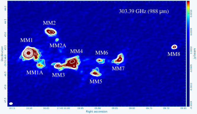
Figure 1: Continuum emission image of high-mass star-formation region G358.93–0.03 at a wavelength of 988 $\mu$m. The synthesized beam size (white circle) of the continuum image is 0.412^′′$\times$0.363^′′. The sub-millimeter continuum sources MM1–MM8 are located in the massive star-formation region G358.93–0.03. The contour (white colour) levels start at 3$\sigma$ where $\sigma$ is the RMS of the continuum emission image and the contour levels increase by a factor of $\surd$2.

The chemistry of hot cores is characterized by the sublimation of ice mantles, which accumulate during the star formation process (Shimonishi et al., 2021). In prestellar cores and cold molecular clouds, the atoms and gaseous molecules freeze onto the dust grains. During the process of star-formation, the thermal energy and pressure increase due to the gravitational collapse. Therefore, dust temperatures also increase, and chemical interactions between heavy species become active on the grain surfaces (Garrod & Herbst, 2006; Shimonishi et al., 2021). This leads to the formation of large complex organic molecules (Garrod & Herbst, 2006; Shimonishi et al., 2021). In addition, sublimated molecules such as ammonia (NH3) and methanol (CH3OH) are also subject to further gas-phase reactions (Nomura & Miller, 2004; Taquet et al., 2016; Shimonishi et al., 2021). Consequently, the warm and dense gas surrounding the protostars becomes chemically rich, resulting in the formation of one of the strongest and most powerful molecular line emitters known as hot molecular cores (Shimonishi et al., 2021). Hot molecular cores are ideal targets for astrochemical studies because a variety of simple and complex organic molecules are frequently found towards these objects (Herbst & van Dishoeck, 2009). They are one of the earliest stages of star formation and play an important role in increasing the chemical complexity of the ISM (Shimonishi et al., 2021). Hot molecular cores are small, compact objects ($\leq$0.1 pc) with a warm temperature ($\geq$100 K) and high gas density ($n_{\ce{H2}}$$\geq$10⁶ cm^-3) that promote molecular evolution by thermal hopping on dust grains (van Dishoeck & Blake, 1998; Williams & Viti, 2014). The lifetime of hot molecular cores is thought to be approximately 10⁵ years (medium warm-up phase) to 10⁶ years (slow warm-up phase) (van Dishoeck & Blake, 1998; Viti et al., 2004; Garrod & Herbst, 2006; Garrod et al., 2008; Garrod, 2013).

The hot molecular core candidate G358.93–0.03 MM1 is located in the high-mass star-formation region G358.93–0.03 at a distance of 6.75$\,\,{}^{\,+0.37}_{\,-0.68}$ kpc (Reid et al., 2014; Brogan et al., 2019). The total gas mass of G358.93–0.03 is 167$\pm$12M_⊙ and its luminosity is $\sim$7.7$\times$10³L_⊙ (Brogan et al., 2019). The high-mass star-formation region G358.93–0.03 contains eight sub-millimeter continuum sources, which are designated as G358.93–0.03 MM1 to G358.93–0.03 MM8 in order of decreasing right ascension (Brogan et al., 2019). G358.93–0.03 MM1 is the brightest sub-millimeter continuum source that hosts a line-rich hot molecular core (Brogan et al., 2019; Bayandina et al., 2022). Previously, maser lines of deuterated water (HDO), isocyanic acid (HNCO), and methanol (CH3OH) were detected towards G358.93–0.03 MM1 using the ALMA, TMRT, and VLA radio telescopes (Brogan et al., 2019; Chen et al., 2020). The rotational emission lines of methyl cyanide (CH3CN) with transition J = 11(4)–10(4) were also detected from both G358.93–0.03 MM1 and G358.93–0.03 MM3 using the ALMA (Brogan et al., 2019). The excitation temperature of CH3CN towards the G358.93–0.03 MM1 and G358.93–0.03 MM3 is 172$\pm$3 K (Brogan et al., 2019). The systematic velocities of G358.93–0.03 MM1 and G358.93–0.03 MM3 are –16.5$\pm$0.3 km s^-1 and –18.6$\pm$0.2 km s^-1, respectively (Brogan et al., 2019). Recently, rotational emission lines of the possible urea precursor molecule cyanamide (NH2CN) were also detected towards G358.93–0.03 MM1 using the ALMA (Manna & Pal, 2023).

In this article, we present the first detection of the simplest sugar-like molecule CH2OHCHO towards the hot molecular core G358.93–0.03 MM1 using the Atacama Large Millimeter/Submillimeter Array (ALMA). ALMA data and their reductions are presented in Section 2. The line identification and the determination of the physical properties of the gas are presented in Section 3. A discussion on the origin of CH2OHCHO in this hot molecular core and conclusions are shown in Section 4 and 5, respectively.

Table 1: Summary of the continuum properties towards G358.93–0.03 at wavelength 988 $\mu$m.

Source	R.A.	Decl.	Deconvolved source size	Integrated flux	Peak flux	RMS	Remark
			(′′$\times$′′)	(mJy)	(mJy beam-1)	($\mu$Jy)
G358.93–0.03 MM1	17:43:10.1015	–29:51:45.7057	0.116$\times$0.085	72.80$\pm$2.20	34.81$\pm$0.75	68.5	Resolved
G358.93–0.03 MM1A	17:43:10.0671	–29:51:46.4511	0.469$\times$0.411	67.71$\pm$2.60	3.53$\pm$0.13	21.1	Resolved
G358.93–0.03 MM2	17:43:10.0357	–29:51:44.9019	0.231$\times$0.088	14.20$\pm$1.40	4.47$\pm$0.35	35.5	Resolved
G358.93–0.03 MM2A	17:43:10.0209	–29:51:45.1577	–	2.30$\pm$0.58	1.52$\pm$0.18	20.3	Not resolved
G358.93–0.03 MM3	17:43:10.0145	–29:51:46.1933	0.072$\times$0.019	6.12$\pm$0.32	5.10$\pm$0.16	18.6	Resolved
G358.93–0.03 MM4	17:43:09.9738	–29:51:46.0707	0.160$\times$0.087	10.50$\pm$2.42	4.38$\pm$0.32	49.8	Resolved
G358.93–0.03 MM5	17:43:09.9063	–29.51.46.4814	0.245$\times$0.078	7.80$\pm$1.10	2.50$\pm$0.48	30.4	Resolved
G358.93–0.03 MM6	17:43:09.8962	–29:51:45.9802	0.107$\times$0.062	3.28$\pm$0.21	1.98$\pm$0.08	7.9	Resolved
G358.93–0.03 MM7	17:43:09.8365	–29:51:45.9498	0.216$\times$0.116	13.91$\pm$1.82	3.85$\pm$0.39	38.5	Resolved
G358.93–0.03 MM8	17:43:09.6761	–29:51:45.4688	–	6.50$\pm$0.11	4.582$\pm$0.06	6.4	Not resolved

2 Observations and data reduction

The high-mass star-forming region G358.93–0.03 was observed using the ALMA band 7 receivers (PI: Crystal Brogan). The observation of G358.93–0.03 was performed on October 11, 2019, with a phase center of ($\alpha,\delta$)_J2000 = (17:43:10.000, –29:51:46.000) and an on-source integration time of 756.0 sec. During the observations, a total of 47 antennas were used, with a minimum baseline of 14 m and a maximum baseline of 2517 m. J1550+0527 was used as the flux calibrator and bandpass calibrator, and J1744–3116 was used as the phase calibrator. The observed frequency ranges of G358.93–0.03 were 290.51–292.39 GHz, 292.49–294.37 GHz, 302.62–304.49 GHz, and 304.14–306.01 GHz, with a spectral resolution of 977 kHz (0.963 km s^-1).

We used the Common Astronomy Software Application (CASA 5.4.1) for data reduction and imaging using the ALMA data reduction pipeline (McMullin et al., 2007). We used the Perley-Butler 2017 flux calibrator model for flux calibration using the task SETJY (Perley & Butler, 2017). After the initial data reduction using the CASA pipeline, we utilized task MSTRANSFORM to separate the target data G358.93–0.03 with all the available rest frequencies. The continuum image is created by selecting line-free channels. Before creating the spectral images, the continuum emission is subtracted from the spectral data using the UVCONTSUB task. To create the spectral images of G358.93–0.03, we used Briggs weighting (Briggs, 1995) and a robust value of 0.5. We used the CASA task IMPBCOR to correct the synthesized beam pattern in continuum and spectral images.

3 Results

3.1 Continuum emission

3.1.1 Sub-millimeter wavelength continuum emission towards G358.93–0.03

The continuum emission of G358.93–0.03 is observed at 303.39 GHz (988 $\mu$m), as shown in Figure 1. The synthesized beam size is 0.412^′′$\times$0.363^′′. In the continuum emission image, we observe eight sub-millimeter continuum sources, G358.93–0.03 MM1 to G358.93–0.03 MM8. Among the eight sources, G358.93–0.03 MM1 and G358.93–0.03 MM3 are known as hot molecular cores (Brogan et al., 2019). Additionally, we also detected two other continuum sources associated with G358.93–0.03 MM1 and G358.93–0.03 MM2. We define these two continuum sources as G358.93–0.03 MM1A and G358.93–0.03 MM2A. We individually fit the 2D Gaussian for each source in G358.93–0.03 using the CASA task IMFIT and estimate the integrated flux density, peak flux density, deconvolved source size, and RMS, which are shown in Table 1. Except for G358.93–0.03 MM2A and G358.93–0.03 MM8, we see that the continuum emissions of other sources are resolved. Brogan et al. (2019) also detected the sub-millimeter wavelength continuum emission from the eight individual continuum sources (G358.93–0.03 MM1 to G358.93–0.03 MM8) of G358.93–0.03 at frequencies of 195.58 GHz, 233.75 GHz, and 337.26 GHz.

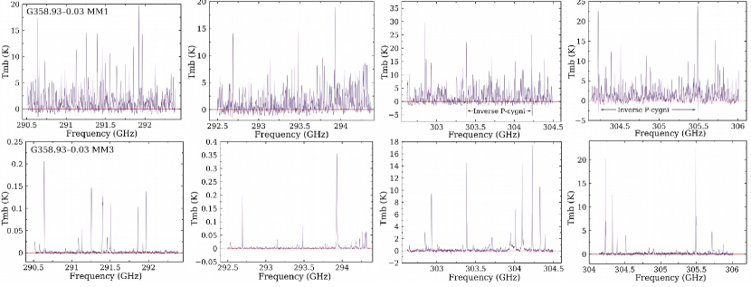
Figure 2: Sub-millimeter wavelength molecular emission spectra towards G358.93–0.03 MM1 (upper panel) and G358.93–0.03 MM3 (lower panel), from ALMA band 7. The spectral resolution of the molecular spectra is 976.56 kHz. The red horizontal lines indicate the baseline of the molecular spectra.

Table 2: Column densities of molecular H2 and optical depths towards the continuum sources in G358.93–0.03.

Source $N_{\ce{H2}}$ $T_{mb}$ $\tau$ (cm^-2) (K) G358.93–0.03 MM1 (3.10$\pm$0.2)$\times$10²⁴ 4.10 27.72$\times$10^-3 G358.93–0.03 MM1A (1.21$\pm$0.8)$\times$10²⁴ 0.41 13.71$\times$10^-3 G358.93–0.03 MM2 (1.53$\pm$0.7)$\times$10²⁴ 0.52 17.66$\times$10^-3 G358.93–0.03 MM2A (5.22$\pm$0.2)$\times$10²³ 0.17   5.93$\times$10^-3 G358.93–0.03 MM3 (3.51$\pm$0.7)$\times$10²³ 0.60   4.01$\times$10^-3 G358.93–0.03 MM4 (1.50$\pm$0.3)$\times$10²⁴ 0.51 17.29$\times$10^-3 G358.93–0.03 MM5 (8.59$\pm$0.5)$\times$10²³ 0.29   9.84$\times$10^-3 G358.93–0.03 MM6 (6.80$\pm$0.6)$\times$10²³ 0.23   7.70$\times$10^-3 G358.93–0.03 MM7 (1.32$\pm$0.5)$\times$10²⁴ 0.45 15.06$\times$10^-3 G358.93–0.03 MM8 (1.57$\pm$0.8)$\times$10²⁴ 0.54 18.13$\times$10^-3

3.1.2 Estimation of molecular hydrogen (H2) column density and optical depth ($\tau$) towards G358.93–0.03

Here we focus on estimating the molecular hydrogen column densities from all continuum sources in G358.93–0.03. The peak flux density ($S_{\nu}$) of the optically thin dust continuum emission can be expressed as

$$S_{\nu}=B_{\nu}(T_{d})\tau_{\nu}\Omega_{beam}$$ (1)

where the Planck function at dust temperature ($T_{d}$) is represented by $B_{\nu}(T_{d})$ (Whittet, 1992), $\tau_{\nu}$ is the optical depth, and $\Omega_{beam}=(\pi/4\ln 2)\times\theta_{major}\times\theta_{minor}$ is the solid angle of the synthesized beam. The expression for the optical depth in terms of the mass density of dust can be written as,

$$\tau_{\nu}=\rho_{d}\kappa_{\nu}L$$ (2)

where $\rho_{d}$ is the mass density of the dust, $\kappa_{\nu}$ is the mass absorption coefficient, and $L$ the path length. The mass density of the dust can be expressed in terms of the dust-to-gas mass ratio ($Z$),

$$\rho_{d}=Z\mu_{H}\rho_{H_{2}}=Z\mu_{H}N_{H_{2}}2m_{H}/L$$ (3)

where $\mu_{H}$ is the mean atomic mass per hydrogen, $\rho_{H_{2}}$ is the hydrogen mass density, $m_{H}$ indicates the mass of hydrogen, and $N_{H_{2}}$ is the column density of hydrogen. For the dust temperature, $T_{d}$, we adopt 150 K, as derived by Chen et al. (2020) for the two hot cores, G358.93–0.03 MM1 and G358.93–0.03 MM3. For the rest of the cores, we adopt a dust temperature of 30.1 K as estimated by Stecklum et al. (2021). We also take $\mu_{H}=1.41$ and $Z=0.01$ (Cox & Pilachowski, 2000). The peak flux density of all the continuum sources in G358.93–0.03 at frequency 303.39 GHz is listed in Table 1. From equations 1, 2, and 3, the column density of molecular hydrogen can be expressed as,

$$N_{H_{2}}=\frac{S_{\nu}/\Omega}{2\kappa_{\nu}B_{\nu}(T_{d})Z\mu_{H}m_{H}}$$ (4)

For the estimation of the mass absorption coefficient ($\kappa_{\nu}$), we use the formula $\kappa_{\nu}=0.90(\nu/230~{}\textrm{GHz})^{\beta}$  cm² g^-1 (Motogi et al., 2019), where $k_{230}=0.90$ cm² g^-1 indicates the emissivity of the dust grains at a gas density of $\rm{10^{6}\ cm^{-3}}$. We use the dust spectral index $\beta$ $\sim$ 1.7 (Brogan et al., 2019). From equation 4, we find the column densities of molecular hydrogen ($N_{\ce{H2}}$) towards all observed continuum sources in G358.93–0.03, which we report in Table 2.

We also determine the value of the dust optical depth ($\tau_{\nu}$) using the following equation,

$$T_{mb}=T_{d}(1-exp(-\tau_{\nu}))$$ (5)

where $T_{mb}$ represents the brightness temperature and $T_{d}$ is the dust temperature. For an estimation of the brightness temperature ($T_{mb}$), we use the Rayleigh-Jeans approximation, 1 Jy beam${}^{-1}\equiv$ 118 K. Using equation 5, we estimate the dust optical depth towards all observed continuum sources in G358.93–0.03 (listed in Table 2). We find that the optical depth of all observed continuum sources is less than 1, indicating that all observed continuum sources in G358.93–0.03 are optically thin at the frequency of 303.39 GHz.

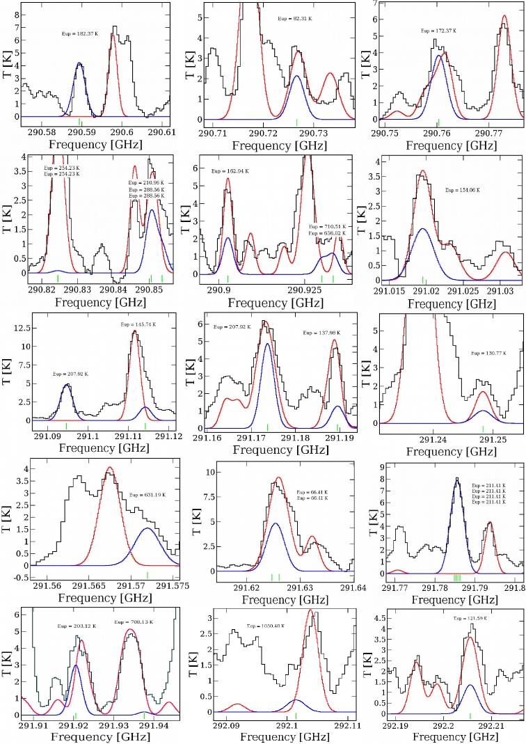
Figure 3: Rotational emission lines of CH2OHCHO towards the hot molecular core G358.93–0.03 MM1. The black spectra are the observations spectra of G358.93–0.03 MM1. The blue spectra represent the LTE model spectrum of just CH2OHCHO, while the red spectra are the LTE model spectra, including all species. The green vertical lines in the LTE spectra indicate the rest frequency positions of the detected transitions of CH2OHCHO.

Figure 3 Continued.

Figure 3 Continued.

Table 3: Summary of the line parameters of CH2OHCHO towards G358.93–0.03 MM1.

Observed frequency Transition $E_{u}$ $A_{ij}$ $G_{up}$ FWHM Optical depth $I_{p}$^† $\rm{\int T_{mb}dV}$ Remark (GHz) (${\rm J^{{}^{\prime}}_{K_{a}^{{}^{\prime}}K_{c}^{{}^{\prime}}}}$–${\rm J^{{}^{\prime\prime}}_{K_{a}^{{}^{\prime\prime}}K_{c}^{{}^{\prime\prime}}}}$) (K) (s^-1) (km s^-1) ($\tau$) (K) (K.km s^-1)   290.589^∗ 18(12,6)–18(11,7) 182.3 2.59$\times$10^-4 37 3.2$\pm$0.2 1.2$\times$10^-2 4.1 11.9$\pm$1.2 Non blended 290.726 15(5,10)–14(4,11)   82.3 2.23$\times$10^-4 31 – 1.3$\times$10^-2 3.6 – Blended with DCOOH   290.760^∗ 17(12,6)–17(11,7) 172.3 2.39$\times$10^-4 35 – 1.0$\times$10^-2 4.8 – Blended with CH3O¹³CHO 290.824 25(11,15)–24(11,14) 254.2 7.78$\times$10^-6 51 – 3.9$\times$10^-4 5.7 – Blended with CH3OCHO 290.824 25(11,14)–24(11,13) 254.2 7.78$\times$10^-6 51 – 3.9$\times$10^-4 5.7 – Blended with CH3OCHO 290.850 26(4,22)–25(5,21) 210.9 3.16$\times$10^-4 53 – 1.9$\times$10^-2 3.7 – Blended with CH3COOH 290.853 33(1,32)–33(0,33) 288.5 6.82$\times$10^-5 67 – 4.0$\times$10^-3 2.5 – Blended with H2CCNH 290.853 33(2,32)–33(1,33) 288.5 6.82$\times$10^-5 67 – 4.0$\times$10^-3 2.5 – Blended with H2CCNH   290.902^∗ 16(12,4)–16(11,5) 162.9 2.16$\times$10^-4 33 – 9.7$\times$10^-3 4.9 – Blended with CH3COOH 290.929 48(9,40)–48(8,41) 710.5 3.81$\times$10^-4 97 – 8.0$\times$10^-3 1.8 – Blended with CH3CH2CN 290.933 44(13,32)–44(12,33) 656.0 4.49$\times$10^-4 89 – 8.2$\times$10^-3 2.8 – Blended with CH3CH2CN   291.019^∗ 15(12,4)–15(11,5) 154.0 1.89$\times$10^-4 31 – 8.1$\times$10^-3 3.5 – Blended with CH3COOH 291.094 27(2,25)–26(3,24) 207.9 5.47$\times$10^-4 55 3.3$\pm$0.3 3.4$\times$10^-2 5.0 14.3$\pm$2.3 Non blended   291.114^∗ 14(12,2)–14(11,3) 145.7 1.55$\times$10^-4 29 – 6.5$\times$10^-3 12.0 – Blended with CH3¹⁸OH 291.173 27(3,25)–26(2,24) 207.9 5.47$\times$10^-4 55 – 3.5$\times$10^-2 5.7 – Blended with CH3CCH   291.189^∗ 13(12,2)–13(11,3) 137.9 1.15$\times$10^-4 27 – 4.5$\times$10^-3 4.5 – Blended with CH3COCH3   291.248^∗ 12(12,0)–12(11,1) 130.7 6.40$\times$10^-5 25 – 2.5$\times$10^-3 2.3 – Blended with HC¹⁸ONH2 291.571 43(13,30)–43(12,31) 631.1 4.47$\times$10^-4 87 – 1.1$\times$10^-2 2.4 – Blended with ¹³CH3CH2CN 291.624 11(7,5)–10(6,4)   66.4 4.49$\times$10^-4 23 – 2.0$\times$10^-2 8.9 – Blended with DCONH2 291.626 11(7,4)–10(6,5)   66.4 4.49$\times$10^-4 23 – 2.0$\times$10^-2 8.9 – Blended with DCONH2 291.784 28(1,27)–27(2,26) 211.4 6.46$\times$10^-4 57 3.4$\pm$0.1 4.2$\times$10^-2 8.1 27.9$\pm$4.8 Non blended 291.784 28(2,27)–27(2,26) 211.4 9.58$\times$10^-6 57 3.4$\pm$0.1 4.2$\times$10^-2 8.1 27.9$\pm$4.8 Non blended 291.784 28(1,27)–27(1,26) 211.4 9.58$\times$10^-6 57 3.4$\pm$0.1 4.2$\times$10^-2 8.1 27.9$\pm$4.8 Non blended 291.786 28(2,27)–27(1,26) 211.4 6.46$\times$10^-4 57 3.4$\pm$0.1 4.2$\times$10^-2 8.1 27.9$\pm$4.9 Non blended 291.920 26(4,23)–25(3,22) 203.1 4.41$\times$10^-4 53 – 2.8$\times$10^-2 4.7 – Blended with ¹³CH2CHCN 291.937 47(11,37)–46(12,34) 708.1 8.68$\times$10^-5 95 – 1.8$\times$10^-3 4.8 – Blended with CH3COOH 292.101 58(11,47)–58(10,48) 1050.4 4.50$\times$10^-4 117 – 3.7$\times$10^-3 1.5 – Blended with C2H5OH 292.205 19(5,15)–18(4,14) 121.5 2.13$\times$10^-4 39 – 1.2$\times$10^-2 4.2 – Blended with E-CH3CHO 292.314 41(5,36)–41(4,37) 498.2 2.79$\times$10^-4 83 – 1.1$\times$10^-2 7.5 – Blended with CH3OCHO 292.536 29(0,29)–28(1,28) 213.6 7.37$\times$10^-4 59 3.3$\pm$0.2 5.0$\times$10^-3 5.3 15.4$\pm$3.5 Non blended 292.536 29(1,29)–28(1,28) 213.6 9.77$\times$10^-6 59 3.3$\pm$0.2 5.0$\times$10^-3 5.3 15.4$\pm$3.5 Non blended 292.536 29(0,29)–28(0,28) 213.6 9.77$\times$10^-6 59 3.3$\pm$0.2 5.0$\times$10^-3 5.3 15.4$\pm$3.5 Non blended 292.536 29(1,29)–28(0,28) 213.6 7.37$\times$10^-4 59 3.3$\pm$0.2 5.0$\times$10^-3 5.3 15.4$\pm$3.5 Non blended 292.737 35(2,33)–35(1,34) 336.7 1.31$\times$10^-4 71 3.2$\pm$0.5 7.0$\times$10^-3 1.3 3.5$\pm$0.1 Non blended 292.737 35(3,33)–35(2,34) 336.7 1.31$\times$10^-4 71 3.2$\pm$0.6 7.0$\times$10^-3 1.3 3.5$\pm$0.1 Non blended 292.924 15(4,11)–14(3,12)   77.6 1.09$\times$10^-4 31 – 6.1$\times$10^-3 1.4 – Blended with CH3C3N 293.257 43(13,31)–43(12,32) 631.1 4.54$\times$10^-4 87 – 1.1$\times$10^-2 1.5 – Blended with HC3N 293.617 39(4,35)–39(3,36) 441.7 2.37$\times$10^-4 79 – 9.8$\times$10^-3 1.0 – Blended with ¹³CH3CH2CN 293.634 39(5,35)–39(4,36) 441.7 2.37$\times$10^-4 79 – 9.8$\times$10^-3 2.5 – Blended with CH3OCH3 293.698 37(3,34)–37(2,35) 387.8 1.88$\times$10^-4 75 – 8.9$\times$10^-3 5.0 – Blended with CH3COOH 293.701 37(4,34)–37(3,35) 387.8 1.88$\times$10^-4 75 – 8.9$\times$10^-3 5.0 – Blended with CH3COOH 293.932 20(5,16)–19(4,15) 132.8 2.21$\times$10^-4 41 – 1.3$\times$10^-2 5.6 – Blended with CH2CH¹³CN 293.951 9(8,2)–8(7,3)   63.8 6.30$\times$10^-4 19 – 2.2$\times$10^-2 5.7 – Blended with ¹³CH3CH2CN 293.951 9(8,1)–8(7,2)   63.8 6.30$\times$10^-4 19 – 2.2$\times$10^-2 5.7 – Blended with ¹³CH3CH2CN 302.698 52(14,39)–52(13,40) 890.6 5.30$\times$10^-4 105 – 6.1$\times$10^-3 6.5 – Blended with CH2DOH 302.761 48(12,36)–47(13,35) 748.6 1.07$\times$10^-4 97 – 1.8$\times$10^-3 6.3 – Blended with HC¹⁸ONH2 302.797 38(13,25)–38(12,36) 515.7 4.70$\times$10^-4 77 – 1.3$\times$10^-2 5.3 – Blended with CH3SH 302.895 66(13,53)–66(12,54) 1362.2 5.32$\times$10^-4 133 – 1.6$\times$10^-3 4.0 – Blended with CH3O¹³CHO 302.911 38(13,26)–38(12,27) 515.7 4.71$\times$10^-4 77 – 1.2$\times$10^-2 15.3 – Blended with CH3OH 302.933 38(3,35)–38(2,36) 407.5 2.09$\times$10^-4 77 – 8.5$\times$10^-3 3.5 – Blended with H¹³CCCN 302.934 38(4,35)–38(3,36) 407.5 2.09$\times$10^-4 77 – 8.5$\times$10^-3 3.5 – Blended with H¹³CCCN 302.962 40(4,36)–40(3,37) 462.7 2.54$\times$10^-4 81 – 9.5$\times$10^-3 2.2 – Blended with CH2CH¹³CN 302.971 40(5,36)–40(4,37) 462.7 2.54$\times$10^-4 81 – 9.5$\times$10^-3 1.5 – Blended with HCOOD 303.089 12(7,6)–11(6,5)   73.0 4.68$\times$10^-4 25 – 2.1$\times$10^-2 7.2 – Blended with NH2CO⁺ 303.094 12(7,5)–11(6,6)   73.0 4.68$\times$10^-4 25 – 2.0$\times$10^-2 6.8 – Blended with c-HCOOH 303.846 27(4,23)–26(5,22) 225.9 3.86$\times$10^-4 55 – 2.1$\times$10^-2 5.2 – Blended with D¹³CCCN 304.347 37(13,24)–37(12,25) 494.4 4.71$\times$10^-4 75 – 1.4$\times$10^-2 3.3 – Blended with CH3CDO 304.409 37(13,25)–37(12,26) 494.4 4.71$\times$10^-4 75 – 1.4$\times$10^-2 5.3 – Blended with NCHCCO 304.509 26(9,18)–25(9,16) 245.0 9.75$\times$10^-6 53 – 4.8$\times$10^-4 0.5 – Blended with ¹³CH3CN 304.574 26(9,17)–25(9,16) 245.0 9.76$\times$10^-6 53 – 4.8$\times$10^-4 0.3 – Blended with C2H5C¹⁵N 304.609 61(14,48)–61(13,49) 1182.5 5.58$\times$10^-4 123 – 2.8$\times$10^-3 0.8 – Blended with C2H5CN 304.612 61(17,45)–60(18,42) 1232.1 1.07$\times$10^-4 123 – 4.6$\times$10^-4 0.8 – Blended with C2H5CN 304.895 25(6,19)–24(6,18) 206.1 1.05$\times$10^-5 51 – 5.7$\times$10^-4 0.9 – Blended with H¹³CCN 304.930 33(7,26)–32(8,25) 350.1 1.50$\times$10^-4 67 – 6.6$\times$10^-3 4.9 – Blended with CH3OCHO 304.954 39(9,30)–38(10,29) 491.1 1.17$\times$10^-4 79 – 3.8$\times$10^-3 1.8 – Blended with HC(O)NH2 305.040 47(7,40)–47(6,41) 670.3 3.90$\times$10^-4 95 3.4$\pm$0.6 6.1$\times$10^-3 1.6 5.806$\pm$1.87 Non blended 305.106 52(10,43)–52(9,44) 836.5 4.59$\times$10^-4 105 – 3.1$\times$10^-3 0.7 – Blended with CH3COOH 305.113 26(6,21)–25(6,20) 218.9 1.05$\times$10^-5 53 – 2.6$\times$10^-4 3.0 – Blended with C2H5CN

Table 2 Continued.

Observed frequency Transition $E_{u}$ $A_{ij}$ $G_{up}$ FWHM Optical depth $I_{p}$^† $\rm{\int T_{mb}dV}$ Remark (GHz) (${\rm J^{{}^{\prime}}_{K_{a}^{{}^{\prime}}K_{c}^{{}^{\prime}}}}$–${\rm J^{{}^{\prime\prime}}_{K_{a}^{{}^{\prime\prime}}K_{c}^{{}^{\prime\prime}}}}$) (K) (s^-1) (km s^-1) ($\tau$) (K) (K km s^-1) 305.203 51(14,38)–51(13,39) 861.2 5.38$\times$10^-4 103 – 3.1$\times$10^-3 3.2 – Blended with CH2DCHO 305.483 16(5,11)–15(4,12)   91.4 2.29$\times$10^-4 33 – 5.4$\times$10^-3 3.9 – Blended with CH3COOH 305.488^∗ 10(8,3)–9(7,2)   69.4 6.41$\times$10^-4 21 3.4$\pm$0.5 1.1$\times$10^-2 6.2 24.2$\pm$2.6 Non blended 305.669 57(15,42)–57(14,43) 1062.5 5.56$\times$10^-4 115 – 1.9$\times$10^-3 1.4 – Blended with CH3COOH 305.700 47(8,40)–47(7,41) 670.3 3.93$\times$10^-4 95 – 4.1$\times$10^-3 15.6 – Blended with CH2DCHO 305.740 36(13,23)–36(12,24) 473.6 4.71$\times$10^-4 73 – 7.0$\times$10^-3 3.5 – Blended with CH3COOH 305.773 36(13,24)–36(12,25) 473.6 4.71$\times$10^-4 73 – 7.0$\times$10^-3 2.5 – Blended with CH3¹⁸OH

*– There are two transitions that have close frequencies ($\leq 100$ kHz), and only the frequency of the first transition is shown.
$\dagger$–$I_{p}$ is the peak intensity of the emission lines of CH2OHCHO.

3.2 Line emission from G358.93–0.03

From the spectral images of G358.93–0.03, we see that only the spectra of G358.93–0.03 MM1 and G358.93–0.03 MM3 show any line emission. The synthesized beam sizes of the spectral images of G358.93–0.03 at frequency ranges of 290.51–292.39 GHz, 292.49–294.37 GHz, 302.62–304.49 GHz, and 304.14–306.01 GHz are 0.425${}^{\prime\prime}\times$0.369^′′, 0.427${}^{\prime\prime}\times$0.376^′′, 0.413${}^{\prime\prime}\times$0.364^′′, and 0.410${}^{\prime\prime}\times$0.358^′′, respectively. We extract the molecular spectra from G358.93–0.03 MM1 and G358.93–0.03 MM3 by drawing a 0.912^′′ diameter circular region, which is larger than the line emitting regions of G358.93–0.03 MM1 and G358.93–0.03 MM3. The phase centre of G358.93–0.03 MM1 is RA (J2000) = 17^h43^m10^s.101, Dec (J2000) = –29^∘51^′45^′′.693. The phase centre of G358.93–0.03 MM3 is RA (J2000) = 17^h43^m10^s.0144, Dec (J2000) = –29^∘51^′46^′′.193. The resultant spectra of G358.93–0.03 MM1 and G358.93–0.03 MM3 are shown in Figure 2. From the spectra, it can be seen that G358.93–0.03 MM1 is more chemically rich than G358.93–0.03 MM3. Additionally, we also observe the signature of an inverse P-Cygni profile associated with the CH3OH emission lines towards G358.93–0.03 MM1. This may indicate that the hot molecular core G358.93–0.03 MM1 is undergoing infall. We do not observe any evidence of an inverse P-Cygni profile in the spectra of G358.93–0.03 MM3. The systematic velocities ($V_{LSR}$) of G358.93–0.03 MM1 and G358.93–0.03 MM3 are –16.5 km s^-1 and –18.2 km s^-1, respectively, (Brogan et al., 2019).

3.2.1 Identification of CH2OHCHO towards G358.93–0.03 MM1

To identify the rotational emission lines of CH2OHCHO, we assume local thermodynamic equilibrium (LTE) and use the Cologne Database for Molecular Spectroscopy (CDMS) (Müller et al., 2005). For LTE modelling, we use CASSIS (Vastel et al., 2015). The LTE assumption is valid in the inner region of G358.93–0.03 MM1 because the gas density of the warm inner region of the hot core is 2$\times$10⁷ cm^-3 (Stecklum et al., 2021). To fit the LTE model spectra of CH2OHCHO over the observed molecular spectra, we use the Markov Chain Monte Carlo (MCMC) algorithm in CASSIS. Previously, Gorai et al. (2020) discussed the fitting of the LTE model spectrum using MCMC in detail. We have identified a total of seventy-five transitions of CH2OHCHO towards G358.93–0.03 MM1 between the frequency ranges of 290.51–292.39 GHz, 292.49–294.37 GHz, 302.62–304.49 GHz, and 304.14–306.01 GHz. The upper-level energies of the identified seventy-five transitions of CH2OHCHO vary from 63.86 K to 1362.19 K. Among the detected seventy-five transitions, we find that only fourteen transitions of CH2OHCHO are not blended, and these lines are identified to be higher than 4$\sigma$ (confirmed from LTE modelling). The upper-level energies of the non-blended transitions of CH2OHCHO vary between 69.40 K and 670.33 K. There are no missing transitions in CH2OHCHO in the observed frequency ranges. The blended transitions of CH2OHCHO will not be considered in our modelling. From the LTE modelling, the best-fit column density of CH2OHCHO is found to be (1.52$\pm$0.9)$\times$10¹⁶ cm^-2 with an excitation temperature of 300$\pm$68.5 K and a source size of 0.45^′′. The FWHM of the LTE spectra of CH2OHCHO is 3.35 km s^-1. We observed that the FWHM of the spectra of CH2OHCHO is nearly similar to the FWHM of another molecule CH3CN towards G358.93–0.03 MM1, which was estimated by Brogan et al. (2019). The LTE-fitted rotational emission spectra of CH2OHCHO are shown in Figure 3. In addition to CH2OHCHO, the hot molecular core G358.93–0.03 MM1 also contains several other complex organic molecules, including CH3OCHO, CH3COOH, CH3NH2, CH3OH, CH3SH, C2H5CN, and C2H3CN, which we discuss in a separate paper.

We report the details of all the detected CH2OHCHO lines in Table 3. Additionally, we also fitted the Gaussian model over the non-blended emission lines of CH2OHCHO to estimate the proper full width-half maximum (FWHM) in km s^-1 and integrated intensity ($\rm{\int T_{mb}dV}$) in K km s^-1. We have observed three different non-blended emission lines of CH2OHCHO at frequencies of 291.784 GHz, 292.536 GHz, and 292.737 GHz that contain multiple transitions of CH2OHCHO. These transitions are reported in Table 3. We cannot separate these observed transitions as they are very close to each other, i.e., blended with each other. To obtain the line parameters of those transitions of CH2OHCHO, we have fitted a multiple-component Gaussian using the Levenberg-Marquardt algorithm in CASSIS to the observed spectra. For multiple Gaussian fittings, we have used fixed values of velocity separation and the expected line intensity ratio. During the fitting of a multi-component Gaussian, only the FWHM is kept as a free parameter. This method works well in the observed spectral profiles around 291.784 GHz, 292.536 GHz, and 292.737 GHz of CH2OHCHO. The summary of the detected transitions and spectral line properties of CH2OHCHO is presented in Table 3.

To determine the fractional abundance of CH2OHCHO, we use the column density of CH2OHCHO inside the 0.45^′′ beam, and divide it by the H2 column density found in Section 3.1.2. The fractional abundance of CH2OHCHO with respect to H2 towards the G358.93–0.03 MM1 is (4.90$\pm$2.92)$\times$10^-9, where the column density of H2 towards the G358.93–0.03 MM1 is (3.10$\pm$0.2)$\times$10²⁴ cm^-2. Recently, Mininni et al. (2020) found that the abundance of CH2OHCHO towards another hot molecular core, G31.41+0.31, was (5.0$\pm$1.4)$\times$10^-9, which is close to our derived abundance of CH2OHCHO towards G358.93–0.03 MM1. This indicates that the chemical formation route(s) of CH2OHCHO towards the G358.93–0.03 MM1 may be similar to those in G31.41+0.31.

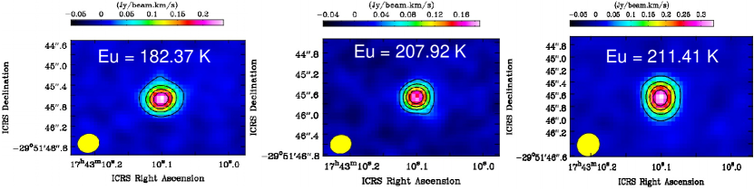
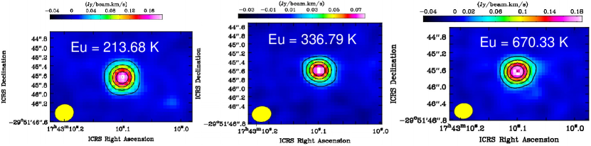
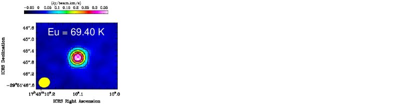
Figure 4: Integrated emission maps (moment zero) of CH2OHCHO towards G358.93–0.03 MM1. The contour levels are at 20%, 40%, 60%, and 80% of the peak flux. Yellow circles represent the synthesized beams of the integrated emission maps.

3.2.2 Searching for CH2OHCHO towards G358.93–0.03 MM3

After the successful detection of CH2OHCHO in G358.93–0.03 MM1, we also search for emission lines of CH2OHCHO towards G358.93–0.03 MM3, which yield no detection. The derived upper-limit column density of CH2OHCHO towards this core is $\leq$(3.52$\pm$1.2)$\times$10¹⁵ cm^-2. The upper limit of the fractional abundance is $\leq$(1.01$\pm$0.40)$\times$10^-8.

3.3 Spatial distribution of CH2OHCHO towards G358.93–0.03 MM1

We create the integrated emission maps (moment zero maps) of CH2OHCHO towards G358.93–0.03 MM1 using the CASA task IMMOMENTS. In task IMMOMENTS, we use channels corresponding to the velocity ranges, where the emission lines of CH2OHCHO were detected. The integrated emission maps are shown in Figure 4. After the extraction, we apply the CASA task IMFIT to fit the 2D Gaussian over the integrated emission maps of CH2OHCHO to estimate the size of the emitting regions. The following equation is used

$$~~~~\theta_{S}=\sqrt{\theta^{2}_{50}-\theta^{2}_{\text{beam}}}$$ (6)

where $\theta_{\text{beam}}$ is the half-power width of the synthesized beam and $\theta_{50}=2\sqrt{A/\pi}$ denotes the diameter of the circle whose area is surrounded by the $50\%$ line peak of CH2OHCHO (Rivilla et al., 2017). The derived sizes of the emitting regions of CH2OHCHO and velocity ranges at different frequencies are listed in Table 4. The synthesized beam sizes of the integrated emission maps are 0.425${}^{\prime\prime}\times$0.369^′′, 0.427${}^{\prime\prime}\times$0.376^′′, 0.413${}^{\prime\prime}\times$0.364^′′, and 0.410${}^{\prime\prime}\times$0.358^′′, respectively. We observe that the estimated emitting region of CH2OHCHO is comparable to or slightly greater than the synthesized beam sizes of the integrated emission maps. This indicates that the detected CH2OHCHO transition lines are not spatially resolved or are only marginally resolved towards G358.93–0.03 MM1. Hence, we cannot draw any conclusions regarding the morphology of the spatial distributions of CH2OHCHO. Higher spatial and angular resolution observations are required to understand the spatial distribution of CH2OHCHO towards G358.93–0.03 MM1.

4 Discussion

In this section, we compare the derived abundance of CH2OHCHO in G358.93–0.03 MM1 with that of other hot cores and corinos. We also discuss the possible pathways for the formation of CH2OHCHO in the context of hot molecular cores. Finally, we compare the observed abundance with those derived from chemical models.

4.1 Comparison with other sources

We list the abundances of CH2OHCHO towards IRAS 16293–2422 B, NGC 7129 FIRS 2, NGC 1333 IRAS2A, Sgr B2 (N), G31.41+0.31, and G10.47+0.0 taken from the literature in Table 5. We note that for NGC 1333 IRAS 2A, Coutens et al. (2015) did not actually derive an abundance with respect to H2 but instead with respect to (CH2OH)₂ and CH3OCHO. We, therefore, used their derived column density of CH2OHCHO as well as the column density of H2 as derived by Taquet et al. (2015) to infer an abundance with respect to H2. Using the rotational diagram, Coutens et al. (2015) derived the column density of CH2OHCHO towards NGC 1333 IRAS2A as 2.4$\times$10¹⁵ cm^-2 with a rotational temperature of 130 K. The column density of molecular hydrogen towards NGC 1333 IRAS2A is 5.0$\times$10²⁴ cm^-2 (Taquet et al., 2015). To determine the fractional abundance of CH2OHCHO with respect to H2 towards NGC 1333 IRAS2A, we use the column density of CH2OHCHO, which is divided by the column density of H2. We deduce a fractional abundance for CH2OHCHO towards NGC 1333 IRAS2A with respect to H2 of 4.8$\times$10^-10.

Our estimate for the abundance of CH2OHCHO towards G358.93–0.03 MM1 ((4.90$\pm$2.92)$\times$10^-9) is quite similar to that of the hot molecular core G31.41+0.31 and the hot corino object IRAS 16293–2422 B while approximately one order of magnitude higher than that of G10.47+0.03, Sgr B2 (N), NGC 1333 IRAS 2A, and NGC 7129 FIRS 2. The similarity among G358.93–0.03 MM1, G31.41+0.31, and IRAS 16293–2422 B may indicate that the formation route(s) of CH2OHCHO may be similar in all three sources.

4.2 Possible formation mechanisms of CH2OHCHO towards hot molecular cores and hot corinos

To date, only a few efficient formation pathways of CH2OHCHO have been proposed on grain surfaces in hot molecular cores and hot corinos (Garrod & Herbst, 2006; Garrod et al., 2008; Garrod, 2013; Coutens et al., 2018; Rivilla et al., 2019; Mininni et al., 2020). In the high temperature ($\geq 100$ K) regime, the radicals gain sufficient energy to diffuse across the surface and react to create complex organic molecules (Mininni et al., 2020). Initially, two main formation pathways were proposed for the formation of CH2OHCHO:

HCO + CH2OH$\rightarrow$CH2OHCHO            (1)

and

CH3OH + HCO$\rightarrow$CH2OHCHO+H      (2)

In reaction 1, radical HCO and radical CH2OH react with each other on the grain surfaces to form CH2OHCHO (Garrod et al., 2008; Garrod, 2013; Coutens et al., 2018; Rivilla et al., 2019). This reaction appears to be responsible for the production of CH2OHCHO towards IRAS 16293–2422 B and G31.41+0.31 (Jørgensen et al., 2012; Rivilla et al., 2019; Mininni et al., 2020). In reaction 2, the radicals HCO and CH3OH react with each other on the grain surfaces to produce CH2OHCHO, but this reaction has not yet been tested in a laboratory (Mininni et al., 2020). Initially, Fedoseev et al. (2015) and Chuang et al. (2015) experimentally studied the possible formation pathways of CH2OHCHO on dust grains at low temperatures ($\sim$10 K). The experimental results of Fedoseev et al. (2015) and Chuang et al. (2015) were later confirmed by Simons et al. (2020) by using microscopic kinetic Monte Carlo simulations based on ice chemistry.

Table 4: Estimated emitting regions of CH2OHCHO towards the G358.93–0.03 MM1.

Observed frequency $E_{u}$ emitting region Velocity ranges (GHz) (K) (^′′) (km s^-1)  290.589^∗ 182.37 0.410 –14.29 to –19.61 291.094 207.92 0.412 –13.39 to –18.68 291.784 211.41 0.413 –14.38 to –20.57 292.536 213.68 0.414 –13.35 to –19.31 292.737 336.79 0.415 –14.40 to –19.22 305.040 670.33 0.411 –13.34 to –18.44  305.488^∗  69.40 0.410 –14.14 to –18.79

*–There are two transitions that have close frequencies ($\leq 100$ kHz), and only the frequency of the first transition is shown.

4.3 Chemical modelling of CH2OHCHO in hot molecular cores

To understand the formation mechanisms and abundance of CH2OHCHO in hot molecular cores, Coutens et al. (2018) computed a two-phase warm-up chemical model using the gas grain chemistry code UCLCHEM (Holdship et al., 2017). They assumed a free-fall collapse of a cloud (Phase I), followed by a warm-up phase (Phase II). In the first phase (Phase I), the gas density increased from $n_{H}$ = 300 cm^-3 to 10⁷ cm^-3, and they assumed a constant dust temperature of 10 K. In the second phase (phase II), the gas density remained constant at 10⁷ cm^-3, whereas the dust temperature increased with time from 10 to 300 K. This phase was known as the warm-up phase. In the chemical network used by Coutens et al. (2018), the recombination of the radicals HCO and CH2OH (Reaction 1) dominates the production of CH2OHCHO on the grains. Reaction 1 is the most likely pathway because Butscher et al. (2015) tested this reaction in the laboratory and confirmed that the reaction produced CH2OHCHO. In the warm-up phase, Coutens et al. (2018) showed that the abundance of CH2OHCHO varied from $\sim$10^-9 to 10^-8 (see Figure 3 in Coutens et al. (2018)). Coutens et al. (2018) did not include reaction 2 (recombination of the radical HCO and CH3OH) as earlier work by Woods et al. (2012) showed that by including reaction 2, the estimated model abundance of CH2OHCHO was as high as $\sim$10^-5 (Woods et al., 2012). This modelled abundance of CH2OHCHO by reaction 2 does not match any of the observed abundances in the sample of objects considered here.

4.4 Comparison between observed and chemically modelled abundance of CH2OHCHO

In order to understand the formation pathways of CH2OHCHO towards G358.93–0.03 MM1, we compare our estimated abundance with the modelled ones from Coutens et al. (2018). This comparison is physically reasonable because the dust temperature of this source is 150 K, which is a typical hot core temperature, and the number density (n_H) of this source is $\sim$2$\times$10⁷ cm^-3 (Chen et al., 2020; Stecklum et al., 2021). Hence, the two-phase warm-up chemical model based on the timescales in Coutens et al. (2018) is appropriate for explaining the chemical evolution of CH2OHCHO towards G358.93–0.03 MM1. Coutens et al. (2018) showed that the abundances of CH2OHCHO varies between $\sim$10^-9 and 10^-8. We find that our estimated abundance towards G358.93–0.03 MM1 is (4.90$\pm$2.92)$\times$10^-9, which is in good agreement with the theoretical results in Coutens et al. (2018). This comparison indicates that the simplest sugar-like molecule, CH2OHCHO, may form on the grain surface via the reaction between radical HCO and radical CH2OH (Reaction 1) towards G358.93–0.03 MM1. Of course, the modelled abundance of CH2OHCHO is also similar to the observed abundance of CH2OHCHO towards the hot molecular core G31.41+0.31 and the hot corino object IRAS 16293–2422 B, indicating that reaction 1 may be the most likely pathway for the production of CH2OHCHO towards these two objects too. Radical HCO and radical CH2OH may be created in the ISM by the hydrogenation of CO (CO + H$\rightarrow$HCO^∙+H$\rightarrow$H2CO$\rightarrow$^∙CH2OH) (Hama & Watanabe, 2013). After hydrogenation, radical CH2OH is converted into CH3OH (^∙CH2OH + H$\rightarrow$CH3OH) (Hama & Watanabe, 2013). Our conclusion agrees with the recent work of Mininni et al. (2020), who also found that reaction 1 is the most efficient pathway for the formation of CH2OHCHO towards the hot core G31.41+0.31, as well as other hot molecular cores.

Table 5: Abundance of CH2OHCHO in different objects.

Source X(CH2OHCHO) Refreances Name G358.93–0.03 MM1 (4.90$\pm$2.92)$\times$10^-9 This paper IRAS 16293–2422 B 5.8$\times$10^-9 (Jørgensen et al., 2012) NGC 7129 FIRS 2 5.0$\times$10^-10 (Fuente et al., 2014) NGC 1333 IRAS2A 4.8$\times$10^-10 See section 4.1 Sgr B2 (N) 1.6$\times$10^-10 (Xue et al., 2019) G31.41+0.31 (5.0$\pm$1.4)$\times$10^-9 (Mininni et al., 2020) G10.47+0.03 9.6$\times$10^-10 (Mondal et al., 2021)

5 Conclusions

We present the first detection of CH2OHCHO using ALMA in the hot molecular core G358.93–0.03 MM1. We identify a total of seventy-five transitions of CH2OHCHO, where the upper-level energies vary between 63.86 K and 1362.19 K. The derived abundance of CH3OCHO is (4.90$\pm$2.92)$\times$10^-9. We compare our estimated abundance with that of other hot molecular cores and hot corinos and note that the abundance of CH2OHCHO towards G358.93–0.03 MM1 is quite similar to that found towards another hot molecular core, G31.41+0.31, and the hot corino, IRAS 16293–2422 B (Jørgensen et al., 2012; Mininni et al., 2020). We discuss the possible formation mechanisms of CH2OHCHO in hot molecular cores. We compare our estimated abundance of CH2OHCHO with the theoretical abundance from the chemical model presented in Coutens et al. (2018) and find that they are similar. We conclude that CH2OHCHO is most likely formed via the reaction of radical HCO and radical CH2OH on the grain surfaces in G358.93–0.03 MM1 and other hot molecular cores.

The identification of abundant CH2OHCHO in G358.93–0.03 MM1 suggests that grain surface chemistry is also efficient for the formation of other complex organic molecules in this hot molecular core, including isomers of CH2OHCHO, CH3OCHO and CH3COOH. Indeed, the highly chemically rich spectra and detection of CH2OHCHO towards G358.93–0.03 MM1 make this object another ideal hot core to search for and study other complex organic molecules in star-forming regions. A spectral line study combined with a radiative transfer as well as a two-phase warm-up chemical model is required to understand the prebiotic chemistry of G358.93–0.03 MM1, which will be carried out in our follow-up study.

DATA AVAILABILITY

The plots within this paper and other findings of this study are available from the corresponding author on reasonable request. The data used in this paper are available in the ALMA Science Archive (https://almascience.nrao.edu/asax/), under project code 2019.1.00768.S.

References

- Belloche et al. (2013) Belloche A., Müller H. S. P., Menten K. M., Schilke P., Comit C., 2013, A&A, 559, A47
- Beltrán et al. (2009) Beltrán M. T., Codella C., Viti S., Neri R., Cesaroni R., 2009, ApJL, 690, L93
- Brogan et al. (2019) Brogan C. L., Hunter T. R., Towner A. P. M. et al., 2019, ApJL, 881, L39
- Bayandina et al. (2022) Bayandina O.S., Brogan C.L., Burns, R.A., et al. 2022, AJ, 163(2), p.83
- Butscher et al. (2015) Butscher T., Duvernay F., Theule P., Danger G., Carissan Y., Hagebaum-Reignier D., Chiavassa T., 2015, MNRAS, 453, 1587
- Briggs (1995) Briggs, D. S. 1995, PhD Thesis, New Mex. Inst Min. Tech
- Calcutt et al. (2014) Calcutt H., Viti, S., Codella C., Beltrán M. T., Fontani F., Woods, P. M., 2014, MNRAS, 443, 3157
- Coutens et al. (2018) Coutens A., Viti S., Rawlings J. M. C., et al. 2018, MNRAS, 475, 2
- Coutens et al. (2015) Coutens A., Persson M. V., Jørgensen J. K., Wampfler S. F., Lykke J. M., 2015, A&A, 576, A5
- Chuang et al. (2015) Chuang K. J., Fedoseev G., Ioppolo S., van Dishoeck E. F., & Linnartz H., 2016, MNRAS, 455, 1702
- Cox & Pilachowski (2000) Cox A. N., & Pilachowski C. A., 2000, Physics Today, 53, 77
- Chen et al. (2020) Chen X., Sobolev A. M., Ren Z.-Y., et al. 2020, NatAs, 4, 1170
- Fedoseev et al. (2015) Fedoseev G., Cuppen H. M., Ioppolo S., Lamberts T., & Linnartz H., 2015, MNRAS, 448, 1288
- Fuente et al. (2014) Fuente A., Cernicharo J., Caselli P., et al. 2014, A&A, 568, A65
- Garrod (2013) Garrod R. T., 2013, ApJ, 765, 60
- Garrod & Herbst (2006) Garrod R. T., & Herbst E. 2006., A&A, 457, 927
- Garrod et al. (2008) Garrod R. T., Widicus Weaver S. L., & Herbst E., 2008, ApJ, 682, 283
- Gorai et al. (2020) Gorai P., Bhat B., Sil M., Mondal S. K. Ghosh R., Chakrabarti S. K., Das A., 2020, ApJ, 895, 86
- Hama & Watanabe (2013) Hama T., Watanabe N., 2013, Chem. Rev., 113, 8783
- Holdship et al. (2017) Holdship J., Viti S., Jiménez-Serra I., Makrymallis A., Priestley F., 2017, AJ, 154, 38
- Hollis et al. (2000) Hollis J. M., Lovas F. J., & Jewell P. R., 2000, ApJ, 540, L107
- Hollis et al. (2001) Hollis J. M., Vogel S. N., Snyder L. E., Jewell P. R., & Lovas F. J., 2001, ApJ, 554, L81
- Hollis et al. (2004) Hollis J. M., Jewell P. R., Lovas F. J., & Remijan A., 2004, ApJL, 613, L45
- Halfen et al. (2006) Halfen D. T., Apponi A. J., Woolf N., Polt R., Ziurys L. M., 2006, ApJ, 639, 237
- Herbst & van Dishoeck (2009) Herbst E., & van Dishoeck E. F., 2009, ARA&A, 47, 427
- Jørgensen et al. (2012) Jørgensen J. K., Favre C., Bisschop S. E., Bourke T. L., van Dishoeck E. F., Schmalzl M., 2012, ApJL, 757, L4
- Manna & Pal (2023) Manna, A. & Pal, S., 2023, Astrophys Space Sci, 368, 33, https://doi.org/10.1007/s10509-023-04192-4
- Mondal et al. (2021) Mondal S. K., Gorai P., Sil M., Ghosh R., Etim E. E., Chakrabarti S. K., Shimonishi T., Nakatani N., Furuya K., Tan J. C., Das, A., 2021, ApJ, 922, 194
- McMullin et al. (2007) McMullin J. P., Waters B., Schiebel D., Young W., & Golap K. 2007, in Astronomical Society of the Pacific Conference Series, Vol. 376, Astronomical Data Analysis Software and Systems XVI, ed. R. A. Shaw, F. Hill, & D. J. Bell, 127
- Müller et al. (2005) Müller H. S. P., SchlMder F., Stutzki J. Winnewisser G., 2005, Journal of Molecular Structure, 742, 215
- Mininni et al. (2020) Mininni C. et al., 2020, A&A, 644, A84
- Motogi et al. (2019) Motogi K., Hirota T., Machida M. N., et al. 2019, ApJL, 877, L25
- Nomura & Miller (2004) Nomura H., & Millar T. J., 2004, A&A, 414, 409
- Perley & Butler (2017) Perley R. A., Butler B. J., 2017, ApJ, 230, 1538
- Reid et al. (2014) Reid M. J., Menten K. M., Brunthaler, A., et al. 2014, ApJ, 783, 130
- Rivilla et al. (2017) Rivilla V. M., Beltrán M. T., Cesaroni R., et al. 2017, A&A, 598, A59
- Rivilla et al. (2019) Rivilla V. M., Beltrán M. T., Vasyunin A., et al. 2019, MNRAS, 483, 806
- Shimonishi et al. (2021) Shimonishi T., Izumi N., Furuya K., & Yasui C., 2021, ApJ, 2, 206
- Stecklum et al. (2021) Stecklum B., Wolf V., Linz H., et al., 2021. A&A, 646, p.A161
- Simons et al. (2020) Simons M. A. J., Lamberts T., & Cuppen H. M., 2020, A&A, 634, A52
- Taquet et al. (2015) Taquet, V., Lpez-Sepulcre, A., Ceccarelli, C., et al. 2015, ApJ, 804, 81
- Taquet et al. (2016) Taquet V., Wirstrm E. S., & Charnley S. B. 2016, ApJ, 821, 46
- Vastel et al. (2015) Vastel C., Bottinelli S., Caux E., Glorian J. -M., Boiziot M., 2015, CASSIS: a tool to visualize and analyse instrumental and synthetic spectra. Proceedings of the Annual meeting of the French Society of Astronomy and Astrophysics, 313-316
- Viti et al. (2004) Viti, S., Collings, M. P., Dever, J. W., McCoustra, M. R. S., & Williams, D. A. 2004, MNRAS, 354, 1141
- van Dishoeck & Blake (1998) van Dishoeck E. F. & Blake G. A., 1998, Annu Rev Astron Astrophys, 36, 317
- Woods et al. (2012) Woods P. M., Kelly, G., Viti, S., et al., 2012, APJ, 750, 19
- Whittet (1992) Whittet D. C. B., 1992, Journal of the British Astronomical Association, 102, 230
- Williams & Viti (2014) Williams D. A., Viti S., 2014, Observational Molecular Astronomy: Exploring the Universe Using Molecular Line Emissions. Cambridge Univ. Press, Cambridge
- Xue et al. (2019) Xue C., Remijan A. J., Burkhardt A. M., & Herbst E., 2019, ApJ, 871, 112