\InputIfFileExists

localflags

\excludeversion

conf \includeversionfull \lst@Keynumbersymbol \lst@Keynumbersnone\lstKV@SwitchCases#1none:
left:
right:

CryptoBap: A Binary Analysis Platform for Cryptographic Protocols

Faezeh Nasrabadi 0009-0005-3659-7755 CISPA Helmholtz Center for Information Security faezeh.nasrabadi@cispa.de Robert Künnemann 0000-0003-0822-9283 CISPA Helmholtz Center for Information Security robert.kuennemann@cispa.de  and  Hamed Nemati 0000-0001-9251-3679 CISPA Helmholtz Center for Information Security hamed.nemati@cispa.de
(2023)
Abstract.

We introduce CryptoBap, a platform to verify weak secrecy and authentication for the (ARMv8 and RISC-V) machine code of cryptographic protocols. We achieve this by first transpiling the binary of protocols into an intermediate representation and then performing a crypto-aware symbolic execution to automatically extract a model of the protocol that represents all its execution paths. Our symbolic execution resolves indirect jumps and supports bounded loops using the loop-summarization technique, which we fully automate. The extracted model is then translated into models amenable to automated verification via ProVerif and CryptoVerif using a third-party toolchain. We prove the soundness of the proposed approach and used CryptoBap to verify multiple case studies ranging from toy examples to real-world protocols, TinySSH, an implementation of SSH, and WireGuard, a modern VPN protocol.

This paper uses 𝐜𝐨𝐜𝐨\mathbf{{\color[rgb]{0,0,0}\definecolor[named]{pgfstrokecolor}{rgb}{0,0,0}\pgfsys@color@gray@stroke{0}\pgfsys@color@gray@fill{0}{co}}}𝗅𝗈𝗅𝗈\mathsf{{\color[rgb]{1,0.23,0.13}\definecolor[named]{pgfstrokecolor}{rgb}{1,0.23,0.13}\pgfsys@color@cmyk@stroke{0}{0.77}{0.87}{0}\pgfsys@color@cmyk@fill{0}{0.77}{0.87}{0}{lo}}}𝑟𝑠𝑟𝑠\mathit{{\color[rgb]{0,0.5,1}\definecolor[named]{pgfstrokecolor}{rgb}{0,0.5,1}\pgfsys@color@cmyk@stroke{1}{0.50}{0}{0}\pgfsys@color@cmyk@fill{1}{0.50}{0}{0}{rs}}} to distinguish between different abstraction layers in our modeling and verification (Patrignani, 2020).

Formal Verification, Crypto. Protocols, Security, Binary Analysis
journalyear: 2023copyright: acmlicensedconference: Proceedings of the 2023 ACM SIGSAC Conference on Computer and Communications Security; November 26–30, 2023; Copenhagen, Denmarkbooktitle: Proceedings of the 2023 ACM SIGSAC Conference on Computer and Communications Security (CCS ’23), November 26–30, 2023, Copenhagen, Denmarkprice: 15.00doi: 10.1145/3576915.3623090isbn: 979-8-4007-0050-7/23/11ccs: Security and privacy Logic and verification

1. Introduction

Cryptographic protocols are a vital part of end-user security on the Internet. Therefore, devising techniques to obtain high-assurance guarantees about their correctness and security is highly desirable. Nevertheless, despite the simplicity of such protocols, their design and implementation are notoriously error-prone, and there have been many attacks targeting either their design (e.g., man-in-the-middle attacks like the triple-handshake attack on TLS (Bhargavan et al., 2014)) or implementation (e.g., Heartbleed, CVE-2014-0160).

Formal methods suggest a rigorous foundation to find bugs and provide guarantees about the correctness and security of cryptographic protocols. Rigorous techniques that have been used so far to reason about such protocols belong to two main lines of research. One is based on the Dolev-Yao model, a symbolic model of cryptography (Dolev and Yao, 1981), while the other, the computational approach (Goldwasser and Micali, 1984), is closer to reality and gives stronger and more realistic security assurance.

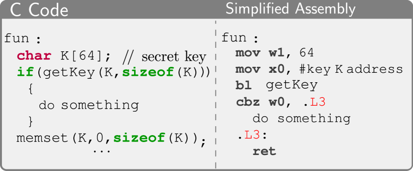
In recent years, significant progress has been made using these techniques to derive rigorous guarantees based on either abstract protocol specifications or the concrete implementations in high-level programming languages such as C or F# (Aizatulin et al., 2012, 2011; Chaki and Datta, 2009; Goubault-Larrecq and Parrennes, 2005; Backes et al., 2010; Bhargavan et al., 2008a). Despite this, there still exists a large gap between the correctness of cryptographic protocols’ models or high-level implementations and their object code (i.e., machine code generated by compilers) that ultimately will execute on hardware. This gap may result in a lack of security, even when correctness proofs are developed for a model or a high-level implementation of the protocol. A major cause for this gap is the fact that program behavior at the source level can diverge from its actual behavior when executed on hardware, e.g., due to compiler-introduced bugs (Xu et al., 2023). This is because enabling aggressive compiler optimizations can lead to missing source-level checks like code intended to detect integer overflows (Wang et al., 2013) or null pointers (Xu et al., 2023). Compilers can invalidate code for secret scrubbing (Sidhpurwala, 2019) or even turn constant-time code into a nonconstant-time binary (Simon et al., 2018). An example is depicted in Fig. 1 where the compiler (GCC ARM V11.2.1) removes the memset function used to erase the secret key from memory. If such a function is part of a protocol specification, its removal can potentially leak the secret key. Alas, even verifying compilers like CompCert (Leroy, 2009) are not a cure-all—verifying all optimization stages that developers want to enjoy in practice is tough.

Refer to caption
Figure 1. An example of how compilers can invalidate code for secret scrubbing

Protocol verification obtains privacy and authenticity guarantees for an abstract model of the protocol that emphasizes concurrency and communication, typically abstracting cryptographic primitives with a fixed set of computation rules for the attacker, known as the Dolev-Yao model (Dolev and Yao, 1981). On the other hand, program verification obtains functional guarantees but also confidentiality in a program model that is typically sequential and focused on a single machine. The attacker is not bound by computation rules or runtime restrictions. Several works have adopted features from one domain in the other—we discuss them in detail in Sec. 2—but this comes at the cost of complex, inflexible execution models and high development cost. We advocate for composing these techniques, thereby bridging the gap between tools and verification technologies that can thus continue to evolve independently.

Our goal in this paper is to extend the verification of security protocols to their machine code. This eliminates the need for trusting compilers and provides a higher assurance about the security and correctness of protocols. To achieve this, we extend HolBA (Lindner et al., 2019) for the verification of RISC-V and ARM binaries with a method for symbolic execution that handles interactions with an arbitrary attacker and trusted cryptographic code. Our symbolic execution resolves indirect jumps and supports (compile-time) bounded loops using the summarization technique (Strejcek and Trtík, 2012), which we fully automate. We also devise a sound translation from symbolic execution to an intermediate layer that is amenable to automated verification with the protocol verifiers ProVerif (Wen et al., 2016; Blanchet, 1 06) and CryptoVerif (Blanchet, 2008)Fig. 2 depicts the pipeline of the CryptoBap.

Implementation-level vulnerabilities like the stack-based buffer overflow in Sami FTP Server 2.0.1 are then covered by the symbolic execution, while protocol-level vulnerabilities like the triple-handshake attack on TLS (Bhargavan et al., 2014) are detected by those protocol verifiers. This is guaranteed by our soundness results and has been evidenced by the discovery of two flaws in CSur and NSL. If there is an error in the implementation of the protocol specification, it could either lead to a model that deviates from the intended behavior, or an error during the extraction process. For instance, if a cryptographic value is erroneously copied within the program, the symbolic execution precisely tracks the memory and detects any subsequent library call operating on the wrongly formatted data. As a result, abstraction would fail, indicating an implementation error; the failure is in the sense that the abstract operations do not apply to incorrectly encoded cryptographic data.

Refer to caption
Figure 2. CryptoBap vs. Csec-modex

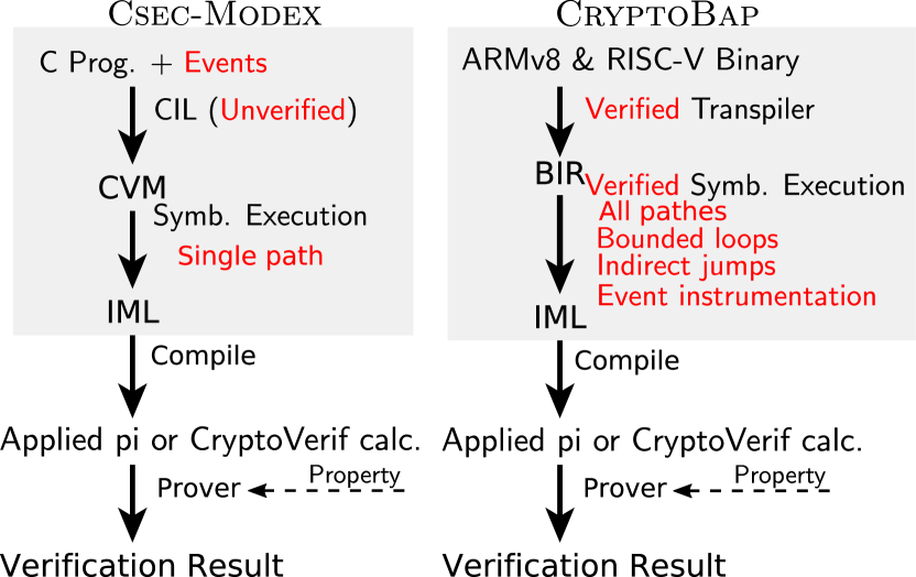
Our method is inspired by and builds on a line of work by Aizatulin et al. (Aizatulin et al., 2012, 2011)Fig. 2 highlights differences between the two approaches (see Sec. 2 for more details on differences of the two approaches.) We adopt their process calculus intermediate model language (𝐼𝑀𝐿𝐼𝑀𝐿\mathit{{\color[rgb]{0,0.5,1}\definecolor[named]{pgfstrokecolor}{rgb}{0,0.5,1}\pgfsys@color@cmyk@stroke{1}{0.50}{0}{0}\pgfsys@color@cmyk@fill{1}{0.50}{0}{0}{{IML}}}}111We depict 𝐁𝐈𝐑𝐁𝐈𝐑\mathbf{{\color[rgb]{0,0,0}\definecolor[named]{pgfstrokecolor}{rgb}{0,0,0}\pgfsys@color@gray@stroke{0}\pgfsys@color@gray@fill{0}{{BIR}}}} in 𝐛𝐥𝐚𝐜𝐤,𝐛𝐨𝐥𝐝𝐫𝐨𝐦𝐚𝐧𝐛𝐥𝐚𝐜𝐤𝐛𝐨𝐥𝐝𝐫𝐨𝐦𝐚𝐧\mathbf{{\color[rgb]{0,0,0}\definecolor[named]{pgfstrokecolor}{rgb}{0,0,0}\pgfsys@color@gray@stroke{0}\pgfsys@color@gray@fill{0}{black,\ bold\ roman}}}, 𝖲𝖡𝖨𝖱𝖲𝖡𝖨𝖱\mathsf{{\color[rgb]{1,0.23,0.13}\definecolor[named]{pgfstrokecolor}{rgb}{1,0.23,0.13}\pgfsys@color@cmyk@stroke{0}{0.77}{0.87}{0}\pgfsys@color@cmyk@fill{0}{0.77}{0.87}{0}{{SBIR}}}} in 𝖱𝖾𝖽𝖮𝗋𝖺𝗇𝗀𝖾,𝗌𝖺𝗇𝗌𝗌𝖾𝗋𝗂𝖿𝖱𝖾𝖽𝖮𝗋𝖺𝗇𝗀𝖾𝗌𝖺𝗇𝗌𝗌𝖾𝗋𝗂𝖿\mathsf{{\color[rgb]{1,0.23,0.13}\definecolor[named]{pgfstrokecolor}{rgb}{1,0.23,0.13}\pgfsys@color@cmyk@stroke{0}{0.77}{0.87}{0}\pgfsys@color@cmyk@fill{0}{0.77}{0.87}{0}{RedOrange,\ sans\ serif}}} and 𝐼𝑀𝐿𝐼𝑀𝐿\mathit{{\color[rgb]{0,0.5,1}\definecolor[named]{pgfstrokecolor}{rgb}{0,0.5,1}\pgfsys@color@cmyk@stroke{1}{0.50}{0}{0}\pgfsys@color@cmyk@fill{1}{0.50}{0}{0}{{IML}}}} in 𝑅𝑜𝑦𝑎𝑙𝐵𝑙𝑢𝑒,𝑡𝑒𝑥𝑡𝑖𝑡𝑎𝑙𝑖𝑐𝑅𝑜𝑦𝑎𝑙𝐵𝑙𝑢𝑒𝑡𝑒𝑥𝑡𝑖𝑡𝑎𝑙𝑖𝑐\mathit{{\color[rgb]{0,0.5,1}\definecolor[named]{pgfstrokecolor}{rgb}{0,0.5,1}\pgfsys@color@cmyk@stroke{1}{0.50}{0}{0}\pgfsys@color@cmyk@fill{1}{0.50}{0}{0}{RoyalBlue,\ text\ italic}}}. Elements common to all languages are typeset in black, italic.) and translation from 𝐼𝑀𝐿𝐼𝑀𝐿\mathit{{\color[rgb]{0,0.5,1}\definecolor[named]{pgfstrokecolor}{rgb}{0,0.5,1}\pgfsys@color@cmyk@stroke{1}{0.50}{0}{0}\pgfsys@color@cmyk@fill{1}{0.50}{0}{0}{{IML}}}} to ProVerif and CryptoVerif. However, we extract the 𝐼𝑀𝐿𝐼𝑀𝐿\mathit{{\color[rgb]{0,0.5,1}\definecolor[named]{pgfstrokecolor}{rgb}{0,0.5,1}\pgfsys@color@cmyk@stroke{1}{0.50}{0}{0}\pgfsys@color@cmyk@fill{1}{0.50}{0}{0}{{IML}}}} model from the machine code of protocols, providing more reliable security guarantees that are independent of the compiler used to generate the object code of protocols. We demonstrate the effectiveness of our approach by covering the case studies of Aizatulin et al. (Aizatulin et al., 2012), including the CSur case study (which they could not verify due to limitations of their framework in handling network messages as C structures), as well as an implementation of SSH called TinySSH (Mojzis, 2018). Moreover, we have verified WireGuard (Donenfeld, 2017), a modern VPN protocol integrated into Linux, by automatically extracting its ProVerif model.

Our threat model includes a set of functions whose input and output behavior are controlled by the attacker. This can represent a network attacker (when these functions are syscalls for network I/O) or a VM running in parallel (when these functions are hypercalls in a security hypervisor, e.g., (Dam et al., 2013; Klein et al., 2010)). The execution platform is trusted to implement the machine-code semantics correctly and includes a set of trusted cryptographic functions. These are likewise assumed to be correct. Also, when outputting to ProVerif, the attacker is assumed to be Dolev-Yao, i.e., cryptography is perfect.

new rules for network communication (Sec. 4, Fig. 8) ARMv8 and RISC-V 𝐁𝐈𝐑𝐁𝐈𝐑\mathbf{{\color[rgb]{0,0,0}\definecolor[named]{pgfstrokecolor}{rgb}{0,0,0}\pgfsys@color@gray@stroke{0}\pgfsys@color@gray@fill{0}{{BIR}}}} 𝖼𝗋𝗒𝗉𝗍𝗈𝖺𝗐𝖺𝗋𝖾𝖼𝗋𝗒𝗉𝗍𝗈𝖺𝗐𝖺𝗋𝖾\mathsf{{\color[rgb]{1,0.23,0.13}\definecolor[named]{pgfstrokecolor}{rgb}{1,0.23,0.13}\pgfsys@color@cmyk@stroke{0}{0.77}{0.87}{0}\pgfsys@color@cmyk@fill{0}{0.77}{0.87}{0}{crypto\!-\!aware}}} 𝖲𝗒𝗆𝖻.𝖤𝗑𝖾𝖼.formulae-sequence𝖲𝗒𝗆𝖻𝖤𝗑𝖾𝖼\mathsf{{\color[rgb]{1,0.23,0.13}\definecolor[named]{pgfstrokecolor}{rgb}{1,0.23,0.13}\pgfsys@color@cmyk@stroke{0}{0.77}{0.87}{0}\pgfsys@color@cmyk@fill{0}{0.77}{0.87}{0}{Symb.Exec.}}} 𝐼𝑀𝐿𝐼𝑀𝐿\mathit{{\color[rgb]{0,0.5,1}\definecolor[named]{pgfstrokecolor}{rgb}{0,0.5,1}\pgfsys@color@cmyk@stroke{1}{0.50}{0}{0}\pgfsys@color@cmyk@fill{1}{0.50}{0}{0}{{IML}}}} CryptoVerif and ProVerif crypto. assumptions on 𝐏𝐏\mathbf{{\color[rgb]{0,0,0}\definecolor[named]{pgfstrokecolor}{rgb}{0,0,0}\pgfsys@color@gray@stroke{0}\pgfsys@color@gray@fill{0}{{P}}}} (Sec. 4): Random number generation Crypto library calls Event function calls verified transpiles to((Lindner et al., 2019, Thm. 2))traces included in(from Thm. 7.6)traces included in(from Thm. 7.3) Csec-modex ((Aizatulin, 2015, Thm. 4.3,Thm. 5.2))attack probabilities are preserved (from Thm. 8.3 using Thm. 7.6Thm. 7.3LABEL:lem:thm4lems) in mixed execution with 𝐼𝑀𝐿𝐼𝑀𝐿\mathit{{\color[rgb]{0,0.5,1}\definecolor[named]{pgfstrokecolor}{rgb}{0,0.5,1}\pgfsys@color@cmyk@stroke{1}{0.50}{0}{0}\pgfsys@color@cmyk@fill{1}{0.50}{0}{0}{{IML}}}} (𝐼𝑀𝐿𝐼𝑀𝐿\mathit{{\color[rgb]{0,0.5,1}\definecolor[named]{pgfstrokecolor}{rgb}{0,0.5,1}\pgfsys@color@cmyk@stroke{1}{0.50}{0}{0}\pgfsys@color@cmyk@fill{1}{0.50}{0}{0}{{IML}}}}𝐁𝐁{}_{\text{$\mathbf{{\color[rgb]{0,0,0}\definecolor[named]{pgfstrokecolor}{rgb}{0,0,0}\pgfsys@color@gray@stroke{0}\pgfsys@color@gray@fill{0}{B}}}$}}, see LABEL:fig:mixedbiriml and 𝐼𝑀𝐿𝐼𝑀𝐿\mathit{{\color[rgb]{0,0.5,1}\definecolor[named]{pgfstrokecolor}{rgb}{0,0.5,1}\pgfsys@color@cmyk@stroke{1}{0.50}{0}{0}\pgfsys@color@cmyk@fill{1}{0.50}{0}{0}{{IML}}}}𝖲𝖡𝖲𝖡{}_{\text{$\mathsf{{\color[rgb]{1,0.23,0.13}\definecolor[named]{pgfstrokecolor}{rgb}{1,0.23,0.13}\pgfsys@color@cmyk@stroke{0}{0.77}{0.87}{0}\pgfsys@color@cmyk@fill{0}{0.77}{0.87}{0}{SB}}}$}}, see Fig. 12) using pure 𝐼𝑀𝐿𝐼𝑀𝐿\mathit{{\color[rgb]{0,0.5,1}\definecolor[named]{pgfstrokecolor}{rgb}{0,0.5,1}\pgfsys@color@cmyk@stroke{1}{0.50}{0}{0}\pgfsys@color@cmyk@fill{1}{0.50}{0}{0}{{IML}}}} semantics (Aizatulin, 2015, p. 23)
Figure 3. Organization of the CryptoBap approach.
Figure 4. Running example. Function addresses are chosen randomly. Line numbers and $pc_{i}$ are addresses of instructions and functions in the memory.

Outline of the CryptoBap’s approach.

As in Fig. 2CryptoBap (source code is available at https://github.com/FMSecure/CryptoBAP) takes as input:

  • the protocol participants’ binary;

  • the symbolic model of cryptographic functions;

  • and, the security property we verify for event traces of executions, formally defined in Sec. 8.

The properties we consider are safety properties over event traces; currently, CryptoBap supports verification of authentication and weak secrecy (Bloch and Barros, 2011). To verify these properties, we transpile the participants’ binary into the 𝐁𝐈𝐑𝐁𝐈𝐑\mathbf{{\color[rgb]{0,0,0}\definecolor[named]{pgfstrokecolor}{rgb}{0,0,0}\pgfsys@color@gray@stroke{0}\pgfsys@color@gray@fill{0}{{BIR}}}} representation, the internal language of the HolBA framework (see Sec. 3.1). Our transpiler is formally verified and guarantees to preserve the semantics of the machine code. However, 𝐁𝐈𝐑𝐁𝐈𝐑\mathbf{{\color[rgb]{0,0,0}\definecolor[named]{pgfstrokecolor}{rgb}{0,0,0}\pgfsys@color@gray@stroke{0}\pgfsys@color@gray@fill{0}{{BIR}}}} as defined in (Lindner et al., 2019) is not suitable for reasoning about the security of cryptographic protocols. We address this by extending 𝐁𝐈𝐑𝐁𝐈𝐑\mathbf{{\color[rgb]{0,0,0}\definecolor[named]{pgfstrokecolor}{rgb}{0,0,0}\pgfsys@color@gray@stroke{0}\pgfsys@color@gray@fill{0}{{BIR}}}} in Sec. 4, e.g., to support network communication, random number generation, etc.

To export the property checking to off-the-shelf verifiers, we extract a model of protocol participants that these verifiers can process. To automate this, we symbolically execute the 𝐁𝐈𝐑𝐁𝐈𝐑\mathbf{{\color[rgb]{0,0,0}\definecolor[named]{pgfstrokecolor}{rgb}{0,0,0}\pgfsys@color@gray@stroke{0}\pgfsys@color@gray@fill{0}{{BIR}}}} translation to instrument on-the-fly the 𝐁𝐈𝐑𝐁𝐈𝐑\mathbf{{\color[rgb]{0,0,0}\definecolor[named]{pgfstrokecolor}{rgb}{0,0,0}\pgfsys@color@gray@stroke{0}\pgfsys@color@gray@fill{0}{{BIR}}}} code with events that flag completion of certain operations and occurrence of errors, and build its execution tree that contains all program execution paths. We translate the resulting execution tree to obtain equivalent programs in 𝐼𝑀𝐿𝐼𝑀𝐿\mathit{{\color[rgb]{0,0.5,1}\definecolor[named]{pgfstrokecolor}{rgb}{0,0.5,1}\pgfsys@color@cmyk@stroke{1}{0.50}{0}{0}\pgfsys@color@cmyk@fill{1}{0.50}{0}{0}{{IML}}}} (see Sec. 3.2 and Sec. 6). The extracted 𝐼𝑀𝐿𝐼𝑀𝐿\mathit{{\color[rgb]{0,0.5,1}\definecolor[named]{pgfstrokecolor}{rgb}{0,0.5,1}\pgfsys@color@cmyk@stroke{1}{0.50}{0}{0}\pgfsys@color@cmyk@fill{1}{0.50}{0}{0}{{IML}}}} model is then passed to Csec-modex (Aizatulin, 2011; Aizatulin et al., 2011), which applies algebraic rewriting to convert the model into the input language of ProVerif and CryptoVerif.

Akin to prior work (Aizatulin et al., 2012, 2011; Chaki and Datta, 2009; Goubault-Larrecq and Parrennes, 2005; Jürjens, 2009; He et al., 2020; Backes et al., 2010; Bhargavan et al., 2008b, a), we trust the cryptographic primitives and abstract them with function symbols that are linked to a Dolev-Yao model when exporting to ProVerif, or to complexity-theoretic assumptions when exporting to CryptoVerif. Analyzing these primitives’ correctness is important, but it requires a different methodology, e.g., weakest precondition propagation. Projects like MSR’s Project Everest (Bhargavan et al., 2017) and the resulting HACL* library (Zinzindohoué et al., 2017), CompCert in conjunction with FCF (Beringer et al., 2015a; Ye et al., 2017) or VALE (Bond et al., 2017) or synthesis approaches like Fiat-Crypto (Erbsen et al., 2020) address this equally challenging problem.

To prove that the extracted 𝐼𝑀𝐿𝐼𝑀𝐿\mathit{{\color[rgb]{0,0.5,1}\definecolor[named]{pgfstrokecolor}{rgb}{0,0.5,1}\pgfsys@color@cmyk@stroke{1}{0.50}{0}{0}\pgfsys@color@cmyk@fill{1}{0.50}{0}{0}{{IML}}}} model preserves the behavior of the actual binary and to relate back the verified properties to the protocol binary, we define a mixed execution semantics. The mixed execution enables protocol participants from different abstraction layers to run in parallel and communicate (see Sec. 7.1 and Fig. 7.2). Such a mixed semantic also frees our symbolic execution from dealing with concurrency. Fig. 3 shows the interconnection between different layers in our approach. To summarize:

  • We present CryptoBap to automate the verification of cryptographic protocols’ binary. Our framework explores all execution paths of protocols, resolves indirect jumps, and handles (compile-time) bounded loops automatically.

  • We extend the vanilla symbolic execution engine in HolBA to automate the model extraction of cryptographic protocols. The way we extend the engine is significant. While HolBA’s vanilla symbolic execution considers the program a holistic entity and thus basically encodes the semantics of the language (𝐁𝐈𝐑𝐁𝐈𝐑\mathbf{{\color[rgb]{0,0,0}\definecolor[named]{pgfstrokecolor}{rgb}{0,0,0}\pgfsys@color@gray@stroke{0}\pgfsys@color@gray@fill{0}{{BIR}}}}), our semantics regards only a part of the whole program and abstracts cryptographic libraries, attacker calls, and random number generation.

  • We formally verify the soundness of our approach and show that verified properties can be transferred back to the binary of analyzed protocols.

  • To evaluate CryptoBap, we have successfully verified multiple case studies, ranging from toy examples, e.g., CSur, to TinySSH and WireGuard.

Running example.

Our running example, Fig. 4, consists of a client and a server that use a symmetric-key encryption scheme to communicate securely. This example shows a weak form of authentication, called aliveness (Lowe, 1997): the server will accept the connection to the (single) client only if it can successfully decrypt the received message using the pre-shared key. First, the client encrypts a message using the shared key, and sends it to the server. Second, the server receives the encrypted message at the other end and decrypts it using the same key. Depending on whether the decryption succeeds or fails, either event_accept, to show acceptance of the connection with the client, or event_bad will be released.

2. Related Work

In the last decade, cryptographers started to employ and even develop theorem provers to develop verifiable proofs (Halevi, 2005). This started with the CertiCrypt framework for Coq (Barthe et al., 1 21), which subsequently developed into EasyCrypt (Barthe et al., 2011). These tools support reasoning about probabilistic programs and classes of (e.g., poly-time restricted) adversaries via probabilistic and probabilistic relational Hoare logic. There are also embeddings of probabilistic reasoning like FCF (Petcher and Morrisett, 5 07), Verypto (Backes et al., 2008) and CryptHOL (Lochbihler, 2016), which are easier to combine with other techniques (this was demonstrated (Beringer et al., 2015b; Petcher and Morrisett, 5 07) for C code), but they require tedious manual analysis and a deep understanding of the underlying relational probabilistic logic.

These methods are typically used to verify cryptographic constructions. By contrast, complex protocols are analyzed using symbolic models, where cryptographic primitives like encryption, signatures, etc. are abstracted using a term algebra and a set of reduction rules. This makes the analysis of protocols that use such primitives amenable to automation, e.g., using first-order SAT solving (Fraikin et al., 2014), Horn clause resolution (Blanchet, 1 06) or constraint solving (Schmidt et al., 2 06). To great success: within a decade, protocol verification tools went from analyzing small academic protocols (Blanchet, 2011; Künnemann and Nemati, 2020) to fully-fledged TLS models (Cremers et al., 0 30; Bhargavan et al., 7 05).

This degree of automation comes at the cost of abstraction, both in terms of the computation environment and the cryptographic primitives. The former is owed to the focus on protocol specifications rather than implementations. This makes sense, because often, the task at hand is to evaluate designs or standards rather than specific implementations, which can be incomplete or nonexistent. There are efforts to translate implementations into the protocol specifications, but they are limited to high-level languages such as C (Aizatulin et al., 2011). The same holds for verification tools that operate at the source-code level (Dupressoir et al., 2014; Küsters et al., 2012).

Papers Language Abstract Model Model Type Property Soundness Aiazatulin et al.(Aizatulin et al., 2012, 2011) C Applied-pi Symb. + Comp. Secrecy, Auth. Chaki et al.(Chaki and Datta, 2009) C ASPIER Symb. Secrecy, Auth. Goubault-Larrecq et al.(Goubault-Larrecq and Parrennes, 2005) C Horn clauses Symb. Secrecy, Info. flow Backes et al.(Backes et al., 2010) F# RFC Symb. + Comp. Safety properties Bhargavan et al.(Bhargavan et al., 2008b, a) F# Pi/CryptoVerif Symb. + Comp. Secrecy, Auth. Jürjens(Jürjens, 2009) Java First-order Logic Symb. Secrecy, Auth. HE et al.(He et al., 2020) Python-JS Applied-pi Symb. Secrecy, Auth. This work Binary Applied-pi Symb. + Comp. Secrecy, Auth.

Table 1. Selected model extraction approaches; Symb = Symbolic, Comp = Computational, Auth = Authentication, JS = JavaScript.

2.1. Verified crypto protocols’ implementation

There have been efforts to verify (annotated) implementations of security protocols using: deductive verification(Dupressoir et al., 2014), type checking (Bhargavan et al., 2010), code generation (Cadé and Blanchet, 2012), and model extraction. Existing work in model extraction mainly targets implementations in high-level languages like C (Chaki and Datta, 2009; Goubault-Larrecq and Parrennes, 2005), F# (Backes et al., 2010; Bhargavan et al., 7 05, 2006) and Java (Jürjens, 2009; O’Shea, 2008). However, due to the complexity of such languages, the existing works have to limit their scope. For example, (Chaki and Datta, 2009) does not model floating pointers and (Goubault-Larrecq and Parrennes, 2005) omits explicit casts and negative array indexes. Table 1 compares selected works that verify the security of protocols via model extraction in some form.

There are also works that recover formats of protocol messages at the binary level (Caballero and Song, 2013; Lin et al., 2008; Wondracek et al., 2008; Xiao et al., 2016). However, their intent is different from ours. Existing approaches are mostly applied to malware binaries and use heuristics to gain insights into their operation. Thus, they are not concerned with soundness, and the inferred message formats can be wrong.

Comparison to Aizatulin et al. approach

Closely related to CryptoBap is Aizatulin’s work (Aizatulin et al., 2011, 2012). Analogous to our work, they also proved the soundness of their approach, i.e., showed that all attacks present in the C code are preserved in the extracted 𝐼𝑀𝐿𝐼𝑀𝐿\mathit{{\color[rgb]{0,0.5,1}\definecolor[named]{pgfstrokecolor}{rgb}{0,0.5,1}\pgfsys@color@cmyk@stroke{1}{0.50}{0}{0}\pgfsys@color@cmyk@fill{1}{0.50}{0}{0}{{IML}}}} models. The main difference between the two approaches is the fact that we target protocols’ binary. Moreover, compared to their approach, which can handle only a single execution path, CryptoBap handles all execution paths of protocols, including those that contain conditionals, bounded loops, and indirect jumps. More specifically, Aizatulin’s approach restricts the input programs to programs that have no “else” branches and no loops. Conceptually, one may see this as irrelevant because one might speculate that all paths outside the “main” part are not useful, i.e., they do not produce network output, or at least none that reveals cryptographic information (e.g., error codes). But this is still restrictive. First, many protocols are specified to produce network output in error cases, for example, decoy messages in anonymity protocols or error messages that are encrypted. Moreover, seemingly regular protocols have “else” branches as part of their “main” message flow, once we look at them with the level of detail necessary to analyze implementations. For example, cypher suite negotiation in TLS must be formulated with multiple branches depending on the input message.

Also, their translation from C to C virtual machine (CVM)—the intermediate language used for extracting the 𝐼𝑀𝐿𝐼𝑀𝐿\mathit{{\color[rgb]{0,0.5,1}\definecolor[named]{pgfstrokecolor}{rgb}{0,0.5,1}\pgfsys@color@cmyk@stroke{1}{0.50}{0}{0}\pgfsys@color@cmyk@fill{1}{0.50}{0}{0}{{IML}}}} model of protocols—is not verified. This renders relating the verified properties to the C implementation infeasible. Similarly, they abstracted cryptographic libraries, attacker calls, and random number generation in their verification. However, they do not formulate the requirements on the program under the analysis explicitly. CVM already assumed to include primitives for library calls, attacker calls, and random number generation—which are not primitives of the C language. In this regard, CVM is fairly close to 𝐼𝑀𝐿𝐼𝑀𝐿\mathit{{\color[rgb]{0,0.5,1}\definecolor[named]{pgfstrokecolor}{rgb}{0,0.5,1}\pgfsys@color@cmyk@stroke{1}{0.50}{0}{0}\pgfsys@color@cmyk@fill{1}{0.50}{0}{0}{{IML}}}}. Moreover, our translation into 𝐼𝑀𝐿𝐼𝑀𝐿\mathit{{\color[rgb]{0,0.5,1}\definecolor[named]{pgfstrokecolor}{rgb}{0,0.5,1}\pgfsys@color@cmyk@stroke{1}{0.50}{0}{0}\pgfsys@color@cmyk@fill{1}{0.50}{0}{0}{{IML}}}} is entirely different (a) because the input language has a more complex state and interaction with the other 𝐼𝑀𝐿𝐼𝑀𝐿\mathit{{\color[rgb]{0,0.5,1}\definecolor[named]{pgfstrokecolor}{rgb}{0,0.5,1}\pgfsys@color@cmyk@stroke{1}{0.50}{0}{0}\pgfsys@color@cmyk@fill{1}{0.50}{0}{0}{{IML}}}} entities and (b) because in contrast to Aizatulin’s approach, we handle conditionals, hence our symbolic execution is not only a sequence of actions. Finally, while they had to change the source code of protocols and add dummy functions to flag the occurrence of events, CryptoBap automates releasing events during symbolic execution and minimizes user involvement.

3. Background

We next explain the preliminaries before presenting the details of our approach.

3.1. HolBA framework & Vanilla symbolic exec.

CryptoBap relies on HolBA (Lindner et al., 2019) to transpile the binary of protocols to the 𝐁𝐈𝐑𝐁𝐈𝐑\mathbf{{\color[rgb]{0,0,0}\definecolor[named]{pgfstrokecolor}{rgb}{0,0,0}\pgfsys@color@gray@stroke{0}\pgfsys@color@gray@fill{0}{{BIR}}}} representation. 𝐁𝐈𝐑𝐁𝐈𝐑\mathbf{{\color[rgb]{0,0,0}\definecolor[named]{pgfstrokecolor}{rgb}{0,0,0}\pgfsys@color@gray@stroke{0}\pgfsys@color@gray@fill{0}{{BIR}}}} is a simple and architecture-agnostic language used as the internal language of HolBA and is designed to simplify the binary analysis of programs and facilitate building analysis tools. HolBA is proof-producing and ensures that the transpilation preserves the semantics of the binary.

𝐏𝐩𝐫𝐨𝐠:=𝐛𝐥𝐨𝐜𝐤𝐛𝐥𝐨𝐜𝐤:=(𝐯,𝐬𝐭𝐦𝐭)𝐯𝐁𝐯𝐚𝐥:=𝑠𝑡𝑟𝑖𝑛𝑔|𝑖𝑛𝑡𝐬𝐭𝐦𝐭:=𝐚𝐬𝐬𝐢𝐠𝐧(𝑠𝑡𝑟𝑖𝑛𝑔,𝐞)|𝐚𝐬𝐬𝐞𝐫𝐭(𝐞)|𝐡𝐚𝐥𝐭|𝐣𝐦𝐩(𝐞)|𝐜𝐣𝐦𝐩(𝐞,𝐞,𝐞)𝐞𝐁𝐞𝐱𝐩:=𝐯|𝐯𝐚𝐫𝑠𝑡𝑟𝑖𝑛𝑔|𝐮𝐞|𝐞𝐛𝐞|𝐢𝐟𝐭𝐡𝐞𝐧𝐞𝐥𝐬𝐞(𝐞,𝐞,𝐞)|𝐥𝐨𝐚𝐝(𝐞,𝐞,𝑖𝑛𝑡)|𝐬𝐭𝐨𝐫𝐞(𝐞,𝐞,𝐞,𝑖𝑛𝑡)\begin{split}\mathbf{{\color[rgb]{0,0,0}\definecolor[named]{pgfstrokecolor}{rgb}{0,0,0}\pgfsys@color@gray@stroke{0}\pgfsys@color@gray@fill{0}{{P}}}}\in\mathbf{{\color[rgb]{0,0,0}\definecolor[named]{pgfstrokecolor}{rgb}{0,0,0}\pgfsys@color@gray@stroke{0}\pgfsys@color@gray@fill{0}{{prog}}}}&\;\;:=\;\;\mathbf{{\color[rgb]{0,0,0}\definecolor[named]{pgfstrokecolor}{rgb}{0,0,0}\pgfsys@color@gray@stroke{0}\pgfsys@color@gray@fill{0}{{block}}}}^{*}\\ \mathbf{{\color[rgb]{0,0,0}\definecolor[named]{pgfstrokecolor}{rgb}{0,0,0}\pgfsys@color@gray@stroke{0}\pgfsys@color@gray@fill{0}{{block}}}}&\;\;:=\;\;({\mathbf{{\color[rgb]{0,0,0}\definecolor[named]{pgfstrokecolor}{rgb}{0,0,0}\pgfsys@color@gray@stroke{0}\pgfsys@color@gray@fill{0}{v}}},\mathbf{{\color[rgb]{0,0,0}\definecolor[named]{pgfstrokecolor}{rgb}{0,0,0}\pgfsys@color@gray@stroke{0}\pgfsys@color@gray@fill{0}{{stmt}}}}^{*}})\\ \mathbf{{\color[rgb]{0,0,0}\definecolor[named]{pgfstrokecolor}{rgb}{0,0,0}\pgfsys@color@gray@stroke{0}\pgfsys@color@gray@fill{0}{v}}}\in\mathbf{{\color[rgb]{0,0,0}\definecolor[named]{pgfstrokecolor}{rgb}{0,0,0}\pgfsys@color@gray@stroke{0}\pgfsys@color@gray@fill{0}{{Bval}}}}&\;\;:=\;\;\mathit{string}\;|\;\mathit{int}\\ \mathbf{{\color[rgb]{0,0,0}\definecolor[named]{pgfstrokecolor}{rgb}{0,0,0}\pgfsys@color@gray@stroke{0}\pgfsys@color@gray@fill{0}{{stmt}}}}&\;\;:=\;\;\mathbf{{\color[rgb]{0,0,0}\definecolor[named]{pgfstrokecolor}{rgb}{0,0,0}\pgfsys@color@gray@stroke{0}\pgfsys@color@gray@fill{0}{assign}}}(\mathit{string},\mathbf{{\color[rgb]{0,0,0}\definecolor[named]{pgfstrokecolor}{rgb}{0,0,0}\pgfsys@color@gray@stroke{0}\pgfsys@color@gray@fill{0}{e}}})\;|\;\mathbf{{\color[rgb]{0,0,0}\definecolor[named]{pgfstrokecolor}{rgb}{0,0,0}\pgfsys@color@gray@stroke{0}\pgfsys@color@gray@fill{0}{assert}}}(\mathbf{{\color[rgb]{0,0,0}\definecolor[named]{pgfstrokecolor}{rgb}{0,0,0}\pgfsys@color@gray@stroke{0}\pgfsys@color@gray@fill{0}{e}}})\;|\;\mathbf{{\color[rgb]{0,0,0}\definecolor[named]{pgfstrokecolor}{rgb}{0,0,0}\pgfsys@color@gray@stroke{0}\pgfsys@color@gray@fill{0}{halt}}}\;|\;\mathbf{{\color[rgb]{0,0,0}\definecolor[named]{pgfstrokecolor}{rgb}{0,0,0}\pgfsys@color@gray@stroke{0}\pgfsys@color@gray@fill{0}{jmp}}}(\mathbf{{\color[rgb]{0,0,0}\definecolor[named]{pgfstrokecolor}{rgb}{0,0,0}\pgfsys@color@gray@stroke{0}\pgfsys@color@gray@fill{0}{e}}})\;\\ &\begin{array}[]{l}\;|\;\;\mathbf{{\color[rgb]{0,0,0}\definecolor[named]{pgfstrokecolor}{rgb}{0,0,0}\pgfsys@color@gray@stroke{0}\pgfsys@color@gray@fill{0}{cjmp}}}(\mathbf{{\color[rgb]{0,0,0}\definecolor[named]{pgfstrokecolor}{rgb}{0,0,0}\pgfsys@color@gray@stroke{0}\pgfsys@color@gray@fill{0}{e}}},\mathbf{{\color[rgb]{0,0,0}\definecolor[named]{pgfstrokecolor}{rgb}{0,0,0}\pgfsys@color@gray@stroke{0}\pgfsys@color@gray@fill{0}{e}}},\mathbf{{\color[rgb]{0,0,0}\definecolor[named]{pgfstrokecolor}{rgb}{0,0,0}\pgfsys@color@gray@stroke{0}\pgfsys@color@gray@fill{0}{e}}})\end{array}\\ \mathbf{{\color[rgb]{0,0,0}\definecolor[named]{pgfstrokecolor}{rgb}{0,0,0}\pgfsys@color@gray@stroke{0}\pgfsys@color@gray@fill{0}{e}}}\in\mathbf{{\color[rgb]{0,0,0}\definecolor[named]{pgfstrokecolor}{rgb}{0,0,0}\pgfsys@color@gray@stroke{0}\pgfsys@color@gray@fill{0}{{Bexp}}}}&\;\;:=\;\;\mathbf{{\color[rgb]{0,0,0}\definecolor[named]{pgfstrokecolor}{rgb}{0,0,0}\pgfsys@color@gray@stroke{0}\pgfsys@color@gray@fill{0}{v}}}\;\;|\;\mathbf{{\color[rgb]{0,0,0}\definecolor[named]{pgfstrokecolor}{rgb}{0,0,0}\pgfsys@color@gray@stroke{0}\pgfsys@color@gray@fill{0}{var}}}\ \mathit{string}\;\;|\;\mathbf{{\color[rgb]{0,0,0}\definecolor[named]{pgfstrokecolor}{rgb}{0,0,0}\pgfsys@color@gray@stroke{0}\pgfsys@color@gray@fill{0}{\Diamond_{u}}}}\mathbf{{\color[rgb]{0,0,0}\definecolor[named]{pgfstrokecolor}{rgb}{0,0,0}\pgfsys@color@gray@stroke{0}\pgfsys@color@gray@fill{0}{e}}}\;\;|\;\mathbf{{\color[rgb]{0,0,0}\definecolor[named]{pgfstrokecolor}{rgb}{0,0,0}\pgfsys@color@gray@stroke{0}\pgfsys@color@gray@fill{0}{e}}}\mathbf{{\color[rgb]{0,0,0}\definecolor[named]{pgfstrokecolor}{rgb}{0,0,0}\pgfsys@color@gray@stroke{0}\pgfsys@color@gray@fill{0}{\Diamond_{b}}}}\mathbf{{\color[rgb]{0,0,0}\definecolor[named]{pgfstrokecolor}{rgb}{0,0,0}\pgfsys@color@gray@stroke{0}\pgfsys@color@gray@fill{0}{e}}}\;|\;\mathbf{{\color[rgb]{0,0,0}\definecolor[named]{pgfstrokecolor}{rgb}{0,0,0}\pgfsys@color@gray@stroke{0}\pgfsys@color@gray@fill{0}{ifthenelse}}}(\mathbf{{\color[rgb]{0,0,0}\definecolor[named]{pgfstrokecolor}{rgb}{0,0,0}\pgfsys@color@gray@stroke{0}\pgfsys@color@gray@fill{0}{e}}},\mathbf{{\color[rgb]{0,0,0}\definecolor[named]{pgfstrokecolor}{rgb}{0,0,0}\pgfsys@color@gray@stroke{0}\pgfsys@color@gray@fill{0}{e}}},\mathbf{{\color[rgb]{0,0,0}\definecolor[named]{pgfstrokecolor}{rgb}{0,0,0}\pgfsys@color@gray@stroke{0}\pgfsys@color@gray@fill{0}{e}}})\\ &\begin{array}[]{l}\;|\;\mathbf{{\color[rgb]{0,0,0}\definecolor[named]{pgfstrokecolor}{rgb}{0,0,0}\pgfsys@color@gray@stroke{0}\pgfsys@color@gray@fill{0}{load}}}(\mathbf{{\color[rgb]{0,0,0}\definecolor[named]{pgfstrokecolor}{rgb}{0,0,0}\pgfsys@color@gray@stroke{0}\pgfsys@color@gray@fill{0}{e}}},\mathbf{{\color[rgb]{0,0,0}\definecolor[named]{pgfstrokecolor}{rgb}{0,0,0}\pgfsys@color@gray@stroke{0}\pgfsys@color@gray@fill{0}{e}}},\!\mathit{int})\;|\;\mathbf{{\color[rgb]{0,0,0}\definecolor[named]{pgfstrokecolor}{rgb}{0,0,0}\pgfsys@color@gray@stroke{0}\pgfsys@color@gray@fill{0}{store}}}(\mathbf{{\color[rgb]{0,0,0}\definecolor[named]{pgfstrokecolor}{rgb}{0,0,0}\pgfsys@color@gray@stroke{0}\pgfsys@color@gray@fill{0}{e}}},\!\mathbf{{\color[rgb]{0,0,0}\definecolor[named]{pgfstrokecolor}{rgb}{0,0,0}\pgfsys@color@gray@stroke{0}\pgfsys@color@gray@fill{0}{e}}},\mathbf{{\color[rgb]{0,0,0}\definecolor[named]{pgfstrokecolor}{rgb}{0,0,0}\pgfsys@color@gray@stroke{0}\pgfsys@color@gray@fill{0}{e}}},\!\mathit{int})\end{array}\end{split}

Figure 5. The 𝐁𝐈𝐑𝐁𝐈𝐑\mathbf{{\color[rgb]{0,0,0}\definecolor[named]{pgfstrokecolor}{rgb}{0,0,0}\pgfsys@color@gray@stroke{0}\pgfsys@color@gray@fill{0}{{BIR}}}} syntax

A 𝐁𝐈𝐑𝐁𝐈𝐑\mathbf{{\color[rgb]{0,0,0}\definecolor[named]{pgfstrokecolor}{rgb}{0,0,0}\pgfsys@color@gray@stroke{0}\pgfsys@color@gray@fill{0}{{BIR}}}} program 𝐏𝐏\mathbf{{\color[rgb]{0,0,0}\definecolor[named]{pgfstrokecolor}{rgb}{0,0,0}\pgfsys@color@gray@stroke{0}\pgfsys@color@gray@fill{0}{{P}}}} includes a number of blocks, see Fig. 5, each consisting of a tuple of a unique label—a string or an integer—and a few statements. Each label refers to a particular location in the program and is often used as the target of jump instructions (i.e., 𝐣𝐦𝐩𝐣𝐦𝐩\mathbf{{\color[rgb]{0,0,0}\definecolor[named]{pgfstrokecolor}{rgb}{0,0,0}\pgfsys@color@gray@stroke{0}\pgfsys@color@gray@fill{0}{jmp}}} or 𝐜𝐣𝐦𝐩𝐜𝐣𝐦𝐩\mathbf{{\color[rgb]{0,0,0}\definecolor[named]{pgfstrokecolor}{rgb}{0,0,0}\pgfsys@color@gray@stroke{0}\pgfsys@color@gray@fill{0}{cjmp}}}). 𝐁𝐈𝐑𝐁𝐈𝐑\mathbf{{\color[rgb]{0,0,0}\definecolor[named]{pgfstrokecolor}{rgb}{0,0,0}\pgfsys@color@gray@stroke{0}\pgfsys@color@gray@fill{0}{{BIR}}}} expressions include constants, standard binary and unary operators (ranged over by 𝐛subscript𝐛\mathbf{{\color[rgb]{0,0,0}\definecolor[named]{pgfstrokecolor}{rgb}{0,0,0}\pgfsys@color@gray@stroke{0}\pgfsys@color@gray@fill{0}{\Diamond_{b}}}} and 𝐮subscript𝐮\mathbf{{\color[rgb]{0,0,0}\definecolor[named]{pgfstrokecolor}{rgb}{0,0,0}\pgfsys@color@gray@stroke{0}\pgfsys@color@gray@fill{0}{\Diamond_{u}}}}) for finite integer arithmetic, memory operations, and conditionals. Fig. 4 presents a 𝐁𝐈𝐑𝐁𝐈𝐑\mathbf{{\color[rgb]{0,0,0}\definecolor[named]{pgfstrokecolor}{rgb}{0,0,0}\pgfsys@color@gray@stroke{0}\pgfsys@color@gray@fill{0}{{BIR}}}} snippet for the running example.

A 𝐁𝐈𝐑𝐁𝐈𝐑\mathbf{{\color[rgb]{0,0,0}\definecolor[named]{pgfstrokecolor}{rgb}{0,0,0}\pgfsys@color@gray@stroke{0}\pgfsys@color@gray@fill{0}{{BIR}}}} state (η,𝐩𝐜)𝐒𝜂𝐩𝐜𝐒(\mathbf{{\color[rgb]{0,0,0}\definecolor[named]{pgfstrokecolor}{rgb}{0,0,0}\pgfsys@color@gray@stroke{0}\pgfsys@color@gray@fill{0}{\eta}}},\mathbf{{\color[rgb]{0,0,0}\definecolor[named]{pgfstrokecolor}{rgb}{0,0,0}\pgfsys@color@gray@stroke{0}\pgfsys@color@gray@fill{0}{{pc}}}})\in\mathbf{{\color[rgb]{0,0,0}\definecolor[named]{pgfstrokecolor}{rgb}{0,0,0}\pgfsys@color@gray@stroke{0}\pgfsys@color@gray@fill{0}{S}}}{} consists of an environment η:𝐁𝐯𝐚𝐫𝐁𝐯𝐚𝐥:𝜂maps-to𝐁𝐯𝐚𝐫𝐁𝐯𝐚𝐥\mathbf{{\color[rgb]{0,0,0}\definecolor[named]{pgfstrokecolor}{rgb}{0,0,0}\pgfsys@color@gray@stroke{0}\pgfsys@color@gray@fill{0}{\eta}}}:\mathbf{{\color[rgb]{0,0,0}\definecolor[named]{pgfstrokecolor}{rgb}{0,0,0}\pgfsys@color@gray@stroke{0}\pgfsys@color@gray@fill{0}{{Bvar}}}}\mapsto\mathbf{{\color[rgb]{0,0,0}\definecolor[named]{pgfstrokecolor}{rgb}{0,0,0}\pgfsys@color@gray@stroke{0}\pgfsys@color@gray@fill{0}{{Bval}}}} which maps variables, i.e., registers 𝐫𝐢subscript𝐫𝐢\mathbf{{\color[rgb]{0,0,0}\definecolor[named]{pgfstrokecolor}{rgb}{0,0,0}\pgfsys@color@gray@stroke{0}\pgfsys@color@gray@fill{0}{r_{i}}}} and memory locations Mem𝑀𝑒𝑚{Mem}, to values and a program counter 𝐩𝐜𝐩𝐜\mathbf{{\color[rgb]{0,0,0}\definecolor[named]{pgfstrokecolor}{rgb}{0,0,0}\pgfsys@color@gray@stroke{0}\pgfsys@color@gray@fill{0}{{pc}}}} that holds the label of the executing 𝐁𝐈𝐑𝐁𝐈𝐑\mathbf{{\color[rgb]{0,0,0}\definecolor[named]{pgfstrokecolor}{rgb}{0,0,0}\pgfsys@color@gray@stroke{0}\pgfsys@color@gray@fill{0}{{BIR}}}} block. The relation 𝐒×𝐒\mathbf{{\color[rgb]{0,0,0}\definecolor[named]{pgfstrokecolor}{rgb}{0,0,0}\pgfsys@color@gray@stroke{0}\pgfsys@color@gray@fill{0}{\xrightarrow[]{\texttt{${\color[rgb]{0,0,0}\definecolor[named]{pgfstrokecolor}{rgb}{0,0,0}\pgfsys@color@gray@stroke{0}\pgfsys@color@gray@fill{0}{}}$}}\mathrel{}_{\texttt{${\color[rgb]{0,0,0}\definecolor[named]{pgfstrokecolor}{rgb}{0,0,0}\pgfsys@color@gray@stroke{0}\pgfsys@color@gray@fill{0}{}}$}}}}}\subseteq\mathbf{{\color[rgb]{0,0,0}\definecolor[named]{pgfstrokecolor}{rgb}{0,0,0}\pgfsys@color@gray@stroke{0}\pgfsys@color@gray@fill{0}{S}}}\times\mathbf{{\color[rgb]{0,0,0}\definecolor[named]{pgfstrokecolor}{rgb}{0,0,0}\pgfsys@color@gray@stroke{0}\pgfsys@color@gray@fill{0}{S}}} models the execution of a 𝐁𝐈𝐑𝐁𝐈𝐑\mathbf{{\color[rgb]{0,0,0}\definecolor[named]{pgfstrokecolor}{rgb}{0,0,0}\pgfsys@color@gray@stroke{0}\pgfsys@color@gray@fill{0}{{BIR}}}} block. The execution of n𝑛{n} steps is denoted by subscriptsuperscript\mathbf{{\color[rgb]{0,0,0}\definecolor[named]{pgfstrokecolor}{rgb}{0,0,0}\pgfsys@color@gray@stroke{0}\pgfsys@color@gray@fill{0}{\xrightarrow[]{\texttt{${\color[rgb]{0,0,0}\definecolor[named]{pgfstrokecolor}{rgb}{0,0,0}\pgfsys@color@gray@stroke{0}\pgfsys@color@gray@fill{0}{}}$}}\mathrel{}^{\texttt{${\color[rgb]{0,0,0}\definecolor[named]{pgfstrokecolor}{rgb}{0,0,0}\pgfsys@color@gray@stroke{0}\pgfsys@color@gray@fill{0}{*}}$}}_{\texttt{${\color[rgb]{0,0,0}\definecolor[named]{pgfstrokecolor}{rgb}{0,0,0}\pgfsys@color@gray@stroke{0}\pgfsys@color@gray@fill{0}{}}$}}}}} if n0𝑛0n\geq 0 and +subscriptsuperscript\mathbf{{\color[rgb]{0,0,0}\definecolor[named]{pgfstrokecolor}{rgb}{0,0,0}\pgfsys@color@gray@stroke{0}\pgfsys@color@gray@fill{0}{\xrightarrow[]{\texttt{${\color[rgb]{0,0,0}\definecolor[named]{pgfstrokecolor}{rgb}{0,0,0}\pgfsys@color@gray@stroke{0}\pgfsys@color@gray@fill{0}{}}$}}\mathrel{}^{\texttt{${\color[rgb]{0,0,0}\definecolor[named]{pgfstrokecolor}{rgb}{0,0,0}\pgfsys@color@gray@stroke{0}\pgfsys@color@gray@fill{0}{+}}$}}_{\texttt{${\color[rgb]{0,0,0}\definecolor[named]{pgfstrokecolor}{rgb}{0,0,0}\pgfsys@color@gray@stroke{0}\pgfsys@color@gray@fill{0}{}}$}}}}} or nsubscriptsuperscript𝑛\mathbf{{\color[rgb]{0,0,0}\definecolor[named]{pgfstrokecolor}{rgb}{0,0,0}\pgfsys@color@gray@stroke{0}\pgfsys@color@gray@fill{0}{\xrightarrow[]{\texttt{${\color[rgb]{0,0,0}\definecolor[named]{pgfstrokecolor}{rgb}{0,0,0}\pgfsys@color@gray@stroke{0}\pgfsys@color@gray@fill{0}{}}$}}\mathrel{}^{\texttt{${\color[rgb]{0,0,0}\definecolor[named]{pgfstrokecolor}{rgb}{0,0,0}\pgfsys@color@gray@stroke{0}\pgfsys@color@gray@fill{0}{n}}$}}_{\texttt{${\color[rgb]{0,0,0}\definecolor[named]{pgfstrokecolor}{rgb}{0,0,0}\pgfsys@color@gray@stroke{0}\pgfsys@color@gray@fill{0}{}}$}}}}}, if n>0𝑛0n>0.

We build CryptoBap on a proof-producing symbolic execution for 𝐁𝐈𝐑𝐁𝐈𝐑\mathbf{{\color[rgb]{0,0,0}\definecolor[named]{pgfstrokecolor}{rgb}{0,0,0}\pgfsys@color@gray@stroke{0}\pgfsys@color@gray@fill{0}{{BIR}}}} (Lindner et al., 2023) that formalizes the symbolic generalization of 𝐁𝐈𝐑𝐁𝐈𝐑\mathbf{{\color[rgb]{0,0,0}\definecolor[named]{pgfstrokecolor}{rgb}{0,0,0}\pgfsys@color@gray@stroke{0}\pgfsys@color@gray@fill{0}{{BIR}}}} (hereafter 𝖲𝖡𝖨𝖱𝖲𝖡𝖨𝖱\mathsf{{\color[rgb]{1,0.23,0.13}\definecolor[named]{pgfstrokecolor}{rgb}{1,0.23,0.13}\pgfsys@color@cmyk@stroke{0}{0.77}{0.87}{0}\pgfsys@color@cmyk@fill{0}{0.77}{0.87}{0}{{SBIR}}}}). The symbolic semantics is bisimilar to the concrete one and allows guiding the execution while maintaining a sound set of reachable states from an initial symbolic state (we call this the symbolic execution structure). To generalize from 𝐁𝐈𝐑𝐁𝐈𝐑\mathbf{{\color[rgb]{0,0,0}\definecolor[named]{pgfstrokecolor}{rgb}{0,0,0}\pgfsys@color@gray@stroke{0}\pgfsys@color@gray@fill{0}{{BIR}}}} to 𝖲𝖡𝖨𝖱𝖲𝖡𝖨𝖱\mathsf{{\color[rgb]{1,0.23,0.13}\definecolor[named]{pgfstrokecolor}{rgb}{1,0.23,0.13}\pgfsys@color@cmyk@stroke{0}{0.77}{0.87}{0}\pgfsys@color@cmyk@fill{0}{0.77}{0.87}{0}{{SBIR}}}}, symbolic expressions 𝖲𝖤𝖲𝖤\mathsf{{\color[rgb]{1,0.23,0.13}\definecolor[named]{pgfstrokecolor}{rgb}{1,0.23,0.13}\pgfsys@color@cmyk@stroke{0}{0.77}{0.87}{0}\pgfsys@color@cmyk@fill{0}{0.77}{0.87}{0}{{SE}}}} are defined that can be interpreted to 𝐁𝐈𝐑𝐁𝐈𝐑\mathbf{{\color[rgb]{0,0,0}\definecolor[named]{pgfstrokecolor}{rgb}{0,0,0}\pgfsys@color@gray@stroke{0}\pgfsys@color@gray@fill{0}{{BIR}}}} values 𝐁𝐯𝐚𝐥𝐁𝐯𝐚𝐥\mathbf{{\color[rgb]{0,0,0}\definecolor[named]{pgfstrokecolor}{rgb}{0,0,0}\pgfsys@color@gray@stroke{0}\pgfsys@color@gray@fill{0}{{Bval}}}} via an interpretation H:𝖲𝖤𝐁𝐯𝐚𝐥:𝐻𝖲𝖤𝐁𝐯𝐚𝐥\mathit{H}:\mathsf{{\color[rgb]{1,0.23,0.13}\definecolor[named]{pgfstrokecolor}{rgb}{1,0.23,0.13}\pgfsys@color@cmyk@stroke{0}{0.77}{0.87}{0}\pgfsys@color@cmyk@fill{0}{0.77}{0.87}{0}{{SE}}}}\to\mathbf{{\color[rgb]{0,0,0}\definecolor[named]{pgfstrokecolor}{rgb}{0,0,0}\pgfsys@color@gray@stroke{0}\pgfsys@color@gray@fill{0}{{Bval}}}}. In addition to the symbolic environment η:𝐁𝐯𝐚𝐫𝖲𝖤:𝜂maps-to𝐁𝐯𝐚𝐫𝖲𝖤\mathsf{{\color[rgb]{1,0.23,0.13}\definecolor[named]{pgfstrokecolor}{rgb}{1,0.23,0.13}\pgfsys@color@cmyk@stroke{0}{0.77}{0.87}{0}\pgfsys@color@cmyk@fill{0}{0.77}{0.87}{0}{\eta}}}:\mathbf{{\color[rgb]{0,0,0}\definecolor[named]{pgfstrokecolor}{rgb}{0,0,0}\pgfsys@color@gray@stroke{0}\pgfsys@color@gray@fill{0}{{Bvar}}}}\mapsto\mathsf{{\color[rgb]{1,0.23,0.13}\definecolor[named]{pgfstrokecolor}{rgb}{1,0.23,0.13}\pgfsys@color@cmyk@stroke{0}{0.77}{0.87}{0}\pgfsys@color@cmyk@fill{0}{0.77}{0.87}{0}{{SE}}}}, the 𝖲𝖡𝖨𝖱𝖲𝖡𝖨𝖱\mathsf{{\color[rgb]{1,0.23,0.13}\definecolor[named]{pgfstrokecolor}{rgb}{1,0.23,0.13}\pgfsys@color@cmyk@stroke{0}{0.77}{0.87}{0}\pgfsys@color@cmyk@fill{0}{0.77}{0.87}{0}{{SBIR}}}} state (ϕ,η,𝐩𝐜)𝖲italic-ϕ𝜂𝐩𝐜𝖲(\mathsf{{\color[rgb]{1,0.23,0.13}\definecolor[named]{pgfstrokecolor}{rgb}{1,0.23,0.13}\pgfsys@color@cmyk@stroke{0}{0.77}{0.87}{0}\pgfsys@color@cmyk@fill{0}{0.77}{0.87}{0}{\phi}}},\mathsf{{\color[rgb]{1,0.23,0.13}\definecolor[named]{pgfstrokecolor}{rgb}{1,0.23,0.13}\pgfsys@color@cmyk@stroke{0}{0.77}{0.87}{0}\pgfsys@color@cmyk@fill{0}{0.77}{0.87}{0}{\eta}}},\mathbf{{\color[rgb]{0,0,0}\definecolor[named]{pgfstrokecolor}{rgb}{0,0,0}\pgfsys@color@gray@stroke{0}\pgfsys@color@gray@fill{0}{{pc}}}})\in\mathsf{{\color[rgb]{1,0.23,0.13}\definecolor[named]{pgfstrokecolor}{rgb}{1,0.23,0.13}\pgfsys@color@cmyk@stroke{0}{0.77}{0.87}{0}\pgfsys@color@cmyk@fill{0}{0.77}{0.87}{0}{{S}}}}{} also contains a path condition ϕ𝖲𝖤italic-ϕ𝖲𝖤\mathsf{{\color[rgb]{1,0.23,0.13}\definecolor[named]{pgfstrokecolor}{rgb}{1,0.23,0.13}\pgfsys@color@cmyk@stroke{0}{0.77}{0.87}{0}\pgfsys@color@cmyk@fill{0}{0.77}{0.87}{0}{\phi}}}\in\mathsf{{\color[rgb]{1,0.23,0.13}\definecolor[named]{pgfstrokecolor}{rgb}{1,0.23,0.13}\pgfsys@color@cmyk@stroke{0}{0.77}{0.87}{0}\pgfsys@color@cmyk@fill{0}{0.77}{0.87}{0}{{SE}}}} and a 𝐩𝐜𝐩𝐜\mathbf{{\color[rgb]{0,0,0}\definecolor[named]{pgfstrokecolor}{rgb}{0,0,0}\pgfsys@color@gray@stroke{0}\pgfsys@color@gray@fill{0}{{pc}}}} that is kept concrete to obtain a concrete control flow.

Let :𝖲×𝖲\mathsf{{\color[rgb]{1,0.23,0.13}\definecolor[named]{pgfstrokecolor}{rgb}{1,0.23,0.13}\pgfsys@color@cmyk@stroke{0}{0.77}{0.87}{0}\pgfsys@color@cmyk@fill{0}{0.77}{0.87}{0}{\xrightarrow[]{\texttt{${\color[rgb]{0,0,0}\definecolor[named]{pgfstrokecolor}{rgb}{0,0,0}\pgfsys@color@gray@stroke{0}\pgfsys@color@gray@fill{0}{}}$}}\mathrel{\mkern-14.0mu}\rightarrow_{\texttt{${\color[rgb]{0,0,0}\definecolor[named]{pgfstrokecolor}{rgb}{0,0,0}\pgfsys@color@gray@stroke{0}\pgfsys@color@gray@fill{0}{}}$}}}}}:\mathsf{{\color[rgb]{1,0.23,0.13}\definecolor[named]{pgfstrokecolor}{rgb}{1,0.23,0.13}\pgfsys@color@cmyk@stroke{0}{0.77}{0.87}{0}\pgfsys@color@cmyk@fill{0}{0.77}{0.87}{0}{{S}}}}\times\mathsf{{\color[rgb]{1,0.23,0.13}\definecolor[named]{pgfstrokecolor}{rgb}{1,0.23,0.13}\pgfsys@color@cmyk@stroke{0}{0.77}{0.87}{0}\pgfsys@color@cmyk@fill{0}{0.77}{0.87}{0}{{S}}}} be the single-step transition relation of 𝖲𝖡𝖨𝖱𝖲𝖡𝖨𝖱\mathsf{{\color[rgb]{1,0.23,0.13}\definecolor[named]{pgfstrokecolor}{rgb}{1,0.23,0.13}\pgfsys@color@cmyk@stroke{0}{0.77}{0.87}{0}\pgfsys@color@cmyk@fill{0}{0.77}{0.87}{0}{{SBIR}}}} and nabsentsubscriptsuperscript𝑛\mathsf{{\color[rgb]{1,0.23,0.13}\definecolor[named]{pgfstrokecolor}{rgb}{1,0.23,0.13}\pgfsys@color@cmyk@stroke{0}{0.77}{0.87}{0}\pgfsys@color@cmyk@fill{0}{0.77}{0.87}{0}{\xrightarrow[]{\texttt{${\color[rgb]{0,0,0}\definecolor[named]{pgfstrokecolor}{rgb}{0,0,0}\pgfsys@color@gray@stroke{0}\pgfsys@color@gray@fill{0}{}}$}}\mathrel{\mkern-14.0mu}\rightarrow^{\texttt{${\color[rgb]{0,0,0}\definecolor[named]{pgfstrokecolor}{rgb}{0,0,0}\pgfsys@color@gray@stroke{0}\pgfsys@color@gray@fill{0}{n}}$}}_{\texttt{${\color[rgb]{0,0,0}\definecolor[named]{pgfstrokecolor}{rgb}{0,0,0}\pgfsys@color@gray@stroke{0}\pgfsys@color@gray@fill{0}{}}$}}}}} (or +absentsubscriptsuperscript\mathsf{{\color[rgb]{1,0.23,0.13}\definecolor[named]{pgfstrokecolor}{rgb}{1,0.23,0.13}\pgfsys@color@cmyk@stroke{0}{0.77}{0.87}{0}\pgfsys@color@cmyk@fill{0}{0.77}{0.87}{0}{\xrightarrow[]{\texttt{${\color[rgb]{0,0,0}\definecolor[named]{pgfstrokecolor}{rgb}{0,0,0}\pgfsys@color@gray@stroke{0}\pgfsys@color@gray@fill{0}{}}$}}\mathrel{\mkern-14.0mu}\rightarrow^{\texttt{${\color[rgb]{0,0,0}\definecolor[named]{pgfstrokecolor}{rgb}{0,0,0}\pgfsys@color@gray@stroke{0}\pgfsys@color@gray@fill{0}{+}}$}}_{\texttt{${\color[rgb]{0,0,0}\definecolor[named]{pgfstrokecolor}{rgb}{0,0,0}\pgfsys@color@gray@stroke{0}\pgfsys@color@gray@fill{0}{}}$}}}}}) denote a multi-step symbolic transition. We write 𝐬𝐢𝐋n𝐬𝐣subscriptsuperscript𝑛𝐋subscript𝐬𝐢subscript𝐬𝐣{\mathbf{{\color[rgb]{0,0,0}\definecolor[named]{pgfstrokecolor}{rgb}{0,0,0}\pgfsys@color@gray@stroke{0}\pgfsys@color@gray@fill{0}{{{s}_{i}}}}}}\mathbf{{\color[rgb]{0,0,0}\definecolor[named]{pgfstrokecolor}{rgb}{0,0,0}\pgfsys@color@gray@stroke{0}\pgfsys@color@gray@fill{0}{\rightarrow}}}^{n}_{\mathbf{{\color[rgb]{0,0,0}\definecolor[named]{pgfstrokecolor}{rgb}{0,0,0}\pgfsys@color@gray@stroke{0}\pgfsys@color@gray@fill{0}{L}}}}{\mathbf{{\color[rgb]{0,0,0}\definecolor[named]{pgfstrokecolor}{rgb}{0,0,0}\pgfsys@color@gray@stroke{0}\pgfsys@color@gray@fill{0}{{{s}_{j}}}}}} to restrict the transition from 𝐬𝐢subscript𝐬𝐢\mathbf{{\color[rgb]{0,0,0}\definecolor[named]{pgfstrokecolor}{rgb}{0,0,0}\pgfsys@color@gray@stroke{0}\pgfsys@color@gray@fill{0}{{{s}_{i}}}}} to 𝐬𝐣subscript𝐬𝐣\mathbf{{\color[rgb]{0,0,0}\definecolor[named]{pgfstrokecolor}{rgb}{0,0,0}\pgfsys@color@gray@stroke{0}\pgfsys@color@gray@fill{0}{{{s}_{j}}}}} to the label set 𝐋𝐋\mathbf{{\color[rgb]{0,0,0}\definecolor[named]{pgfstrokecolor}{rgb}{0,0,0}\pgfsys@color@gray@stroke{0}\pgfsys@color@gray@fill{0}{L}}}. For the HolBA’s vanilla symbolic execution, Lindner et al. (Lindner et al., 2023) proved that a single 𝖲𝖡𝖨𝖱𝖲𝖡𝖨𝖱\mathsf{{\color[rgb]{1,0.23,0.13}\definecolor[named]{pgfstrokecolor}{rgb}{1,0.23,0.13}\pgfsys@color@cmyk@stroke{0}{0.77}{0.87}{0}\pgfsys@color@cmyk@fill{0}{0.77}{0.87}{0}{{SBIR}}}} execution step soundly matches a single 𝐁𝐈𝐑𝐁𝐈𝐑\mathbf{{\color[rgb]{0,0,0}\definecolor[named]{pgfstrokecolor}{rgb}{0,0,0}\pgfsys@color@gray@stroke{0}\pgfsys@color@gray@fill{0}{{BIR}}}} execution step, characterized by the following simulation theorem:

Property 1.

For all 𝐬𝐢,H,𝐬𝐣subscript𝐬𝐢𝐻subscript𝐬𝐣\mathbf{{\color[rgb]{0,0,0}\definecolor[named]{pgfstrokecolor}{rgb}{0,0,0}\pgfsys@color@gray@stroke{0}\pgfsys@color@gray@fill{0}{{{s}_{i}}}}},\mathit{H},\mathbf{{\color[rgb]{0,0,0}\definecolor[named]{pgfstrokecolor}{rgb}{0,0,0}\pgfsys@color@gray@stroke{0}\pgfsys@color@gray@fill{0}{{{s}_{j}}}}}, 𝗌𝗂subscript𝗌𝗂\mathsf{{\color[rgb]{1,0.23,0.13}\definecolor[named]{pgfstrokecolor}{rgb}{1,0.23,0.13}\pgfsys@color@cmyk@stroke{0}{0.77}{0.87}{0}\pgfsys@color@cmyk@fill{0}{0.77}{0.87}{0}{{{s}_{i}}}}} s.t. 𝐬𝐢H𝗌𝗂subscriptsimilar-to𝐻subscript𝐬𝐢subscript𝗌𝗂\mathbf{{\color[rgb]{0,0,0}\definecolor[named]{pgfstrokecolor}{rgb}{0,0,0}\pgfsys@color@gray@stroke{0}\pgfsys@color@gray@fill{0}{{{s}_{i}}}}}\sim_{{}_{\mathit{H}}}{}\mathsf{{\color[rgb]{1,0.23,0.13}\definecolor[named]{pgfstrokecolor}{rgb}{1,0.23,0.13}\pgfsys@color@cmyk@stroke{0}{0.77}{0.87}{0}\pgfsys@color@cmyk@fill{0}{0.77}{0.87}{0}{{{s}_{i}}}}}, if 𝐬𝐢𝐬𝐣subscript𝐬𝐢subscript𝐬𝐣{\mathbf{{\color[rgb]{0,0,0}\definecolor[named]{pgfstrokecolor}{rgb}{0,0,0}\pgfsys@color@gray@stroke{0}\pgfsys@color@gray@fill{0}{{{s}_{i}}}}}}\mathbf{{\color[rgb]{0,0,0}\definecolor[named]{pgfstrokecolor}{rgb}{0,0,0}\pgfsys@color@gray@stroke{0}\pgfsys@color@gray@fill{0}{\rightarrow}}}{\mathbf{{\color[rgb]{0,0,0}\definecolor[named]{pgfstrokecolor}{rgb}{0,0,0}\pgfsys@color@gray@stroke{0}\pgfsys@color@gray@fill{0}{{{s}_{j}}}}}} then there exist an Hsuperscript𝐻\mathit{H}^{\prime} and 𝗌𝗃subscript𝗌𝗃\mathsf{{\color[rgb]{1,0.23,0.13}\definecolor[named]{pgfstrokecolor}{rgb}{1,0.23,0.13}\pgfsys@color@cmyk@stroke{0}{0.77}{0.87}{0}\pgfsys@color@cmyk@fill{0}{0.77}{0.87}{0}{{{s}_{j}}}}} s.t. HH𝐻superscript𝐻\mathit{H}\!\subseteq\!\mathit{H}^{\prime} and 𝗌𝗂𝗌𝗃\mathsf{{\color[rgb]{1,0.23,0.13}\definecolor[named]{pgfstrokecolor}{rgb}{1,0.23,0.13}\pgfsys@color@cmyk@stroke{0}{0.77}{0.87}{0}\pgfsys@color@cmyk@fill{0}{0.77}{0.87}{0}{{{s}_{i}}}}}\mathsf{{\color[rgb]{1,0.23,0.13}\definecolor[named]{pgfstrokecolor}{rgb}{1,0.23,0.13}\pgfsys@color@cmyk@stroke{0}{0.77}{0.87}{0}\pgfsys@color@cmyk@fill{0}{0.77}{0.87}{0}{\xrightarrow[]{\texttt{${\color[rgb]{0,0,0}\definecolor[named]{pgfstrokecolor}{rgb}{0,0,0}\pgfsys@color@gray@stroke{0}\pgfsys@color@gray@fill{0}{}}$}}\mathrel{\mkern-14.0mu}\rightarrow_{\texttt{${\color[rgb]{0,0,0}\definecolor[named]{pgfstrokecolor}{rgb}{0,0,0}\pgfsys@color@gray@stroke{0}\pgfsys@color@gray@fill{0}{}}$}}}}}\mathsf{{\color[rgb]{1,0.23,0.13}\definecolor[named]{pgfstrokecolor}{rgb}{1,0.23,0.13}\pgfsys@color@cmyk@stroke{0}{0.77}{0.87}{0}\pgfsys@color@cmyk@fill{0}{0.77}{0.87}{0}{{{s}_{j}}}}} and 𝐬𝐣H𝗌𝗃subscriptsimilar-tosuperscript𝐻subscript𝐬𝐣subscript𝗌𝗃\mathbf{{\color[rgb]{0,0,0}\definecolor[named]{pgfstrokecolor}{rgb}{0,0,0}\pgfsys@color@gray@stroke{0}\pgfsys@color@gray@fill{0}{{{s}_{j}}}}}\sim_{{}_{\mathit{H}^{\prime}}}{}\mathsf{{\color[rgb]{1,0.23,0.13}\definecolor[named]{pgfstrokecolor}{rgb}{1,0.23,0.13}\pgfsys@color@cmyk@stroke{0}{0.77}{0.87}{0}\pgfsys@color@cmyk@fill{0}{0.77}{0.87}{0}{{{s}_{j}}}}}.

The simulation relation $\sim_{{}_{\mathit{H}}}{}$ asserts the consistency of corresponding 𝐁𝐈𝐑𝐁𝐈𝐑\mathbf{{\color[rgb]{0,0,0}\definecolor[named]{pgfstrokecolor}{rgb}{0,0,0}\pgfsys@color@gray@stroke{0}\pgfsys@color@gray@fill{0}{{BIR}}}} and 𝖲𝖡𝖨𝖱𝖲𝖡𝖨𝖱\mathsf{{\color[rgb]{1,0.23,0.13}\definecolor[named]{pgfstrokecolor}{rgb}{1,0.23,0.13}\pgfsys@color@cmyk@stroke{0}{0.77}{0.87}{0}\pgfsys@color@cmyk@fill{0}{0.77}{0.87}{0}{{SBIR}}}} states, i.e., their program counters are equal, their environments are equal through the interpretation $\mathit{H}$, and the evaluation of ϕitalic-ϕ\mathsf{{\color[rgb]{1,0.23,0.13}\definecolor[named]{pgfstrokecolor}{rgb}{1,0.23,0.13}\pgfsys@color@cmyk@stroke{0}{0.77}{0.87}{0}\pgfsys@color@cmyk@fill{0}{0.77}{0.87}{0}{\phi}}} under $\mathit{H}$ results in $\mathit{true}$. Then the soundness of the symbolic execution structure for multiple steps corresponds to the extension of Property 1 to a multi-step simulation theorem.

3.2. Csec-modex toolchain & 𝐼𝑀𝐿𝐼𝑀𝐿\mathit{{\color[rgb]{0,0.5,1}\definecolor[named]{pgfstrokecolor}{rgb}{0,0.5,1}\pgfsys@color@cmyk@stroke{1}{0.50}{0}{0}\pgfsys@color@cmyk@fill{1}{0.50}{0}{0}{{IML}}}}

Aizatulin et al. (Aizatulin et al., 2011) proposed an automated technique to verify the security of cryptographic protocols’ C implementation. At a high level, Csec-modex takes as input the C code of protocol participants together with a template file for the verifier (ProVerif or CryptoVerif). The toolchain extracts the 𝐼𝑀𝐿𝐼𝑀𝐿\mathit{{\color[rgb]{0,0.5,1}\definecolor[named]{pgfstrokecolor}{rgb}{0,0.5,1}\pgfsys@color@cmyk@stroke{1}{0.50}{0}{0}\pgfsys@color@cmyk@fill{1}{0.50}{0}{0}{{IML}}}} model of the protocol, which is then converted into the verifier’s input language. The template encodes assumptions about cryptographic primitives in the implementation, the environment process which spawns the participants and generates shared cryptographic material, and a query for the security property that is checked for the implementation.

The intermediate model language, 𝐼𝑀𝐿𝐼𝑀𝐿\mathit{{\color[rgb]{0,0.5,1}\definecolor[named]{pgfstrokecolor}{rgb}{0,0.5,1}\pgfsys@color@cmyk@stroke{1}{0.50}{0}{0}\pgfsys@color@cmyk@fill{1}{0.50}{0}{0}{{IML}}}}, is a version of the applied-pi calculus extended with bitstring manipulation primitives.

d,e𝐼𝑒𝑥𝑝:=expressionb𝐵𝑆,x𝐼𝑣𝑎𝑟bitstrings, variables𝑜𝑝(e1,,em)computation,𝑜𝑝𝑂𝑝𝑠P,Q𝐼𝑀𝐿:=process0,P|Qnil, parallel composition!imPreplicating Pm times𝑛𝑒𝑤x:t;Prandomness𝑖𝑛(c[e1,,em],x);Pinput𝑜𝑢𝑡(c[e1,,em],e);Poutput𝑒𝑣𝑒𝑛𝑡(d1,,dm);Pevent𝑖𝑓e𝑡ℎ𝑒𝑛P[𝑒𝑙𝑠𝑒Q]conditional𝑙𝑒𝑡x=e𝑖𝑛Passignment𝑎𝑠𝑠𝑢𝑚𝑒e;Passumption\begin{split}\mathit{{\color[rgb]{0,0.5,1}\definecolor[named]{pgfstrokecolor}{rgb}{0,0.5,1}\pgfsys@color@cmyk@stroke{1}{0.50}{0}{0}\pgfsys@color@cmyk@fill{1}{0.50}{0}{0}{d}}},\mathit{{\color[rgb]{0,0.5,1}\definecolor[named]{pgfstrokecolor}{rgb}{0,0.5,1}\pgfsys@color@cmyk@stroke{1}{0.50}{0}{0}\pgfsys@color@cmyk@fill{1}{0.50}{0}{0}{e}}}&\in\mathit{{\color[rgb]{0,0.5,1}\definecolor[named]{pgfstrokecolor}{rgb}{0,0.5,1}\pgfsys@color@cmyk@stroke{1}{0.50}{0}{0}\pgfsys@color@cmyk@fill{1}{0.50}{0}{0}{{Iexp}}}}\;\;:=\;\;\text{expression}\\ &\begin{array}[]{lll}\mathit{{\color[rgb]{0,0.5,1}\definecolor[named]{pgfstrokecolor}{rgb}{0,0.5,1}\pgfsys@color@cmyk@stroke{1}{0.50}{0}{0}\pgfsys@color@cmyk@fill{1}{0.50}{0}{0}{b}}}\in\mathit{{\color[rgb]{0,0.5,1}\definecolor[named]{pgfstrokecolor}{rgb}{0,0.5,1}\pgfsys@color@cmyk@stroke{1}{0.50}{0}{0}\pgfsys@color@cmyk@fill{1}{0.50}{0}{0}{{BS}}}},\ \mathit{{\color[rgb]{0,0.5,1}\definecolor[named]{pgfstrokecolor}{rgb}{0,0.5,1}\pgfsys@color@cmyk@stroke{1}{0.50}{0}{0}\pgfsys@color@cmyk@fill{1}{0.50}{0}{0}{x}}}\in\mathit{{\color[rgb]{0,0.5,1}\definecolor[named]{pgfstrokecolor}{rgb}{0,0.5,1}\pgfsys@color@cmyk@stroke{1}{0.50}{0}{0}\pgfsys@color@cmyk@fill{1}{0.50}{0}{0}{{Ivar}}}}&&\text{bitstrings,\ variables}\\ \mathit{{\color[rgb]{0,0.5,1}\definecolor[named]{pgfstrokecolor}{rgb}{0,0.5,1}\pgfsys@color@cmyk@stroke{1}{0.50}{0}{0}\pgfsys@color@cmyk@fill{1}{0.50}{0}{0}{{op}}}}(\mathit{{\color[rgb]{0,0.5,1}\definecolor[named]{pgfstrokecolor}{rgb}{0,0.5,1}\pgfsys@color@cmyk@stroke{1}{0.50}{0}{0}\pgfsys@color@cmyk@fill{1}{0.50}{0}{0}{e_{1}}}},\dots,\mathit{{\color[rgb]{0,0.5,1}\definecolor[named]{pgfstrokecolor}{rgb}{0,0.5,1}\pgfsys@color@cmyk@stroke{1}{0.50}{0}{0}\pgfsys@color@cmyk@fill{1}{0.50}{0}{0}{e_{m}}}})&&\text{computation},\mathit{{\color[rgb]{0,0.5,1}\definecolor[named]{pgfstrokecolor}{rgb}{0,0.5,1}\pgfsys@color@cmyk@stroke{1}{0.50}{0}{0}\pgfsys@color@cmyk@fill{1}{0.50}{0}{0}{{op}}}}\in\mathit{{\color[rgb]{0,0.5,1}\definecolor[named]{pgfstrokecolor}{rgb}{0,0.5,1}\pgfsys@color@cmyk@stroke{1}{0.50}{0}{0}\pgfsys@color@cmyk@fill{1}{0.50}{0}{0}{Ops}}}\\ \end{array}\\ \mathit{{\color[rgb]{0,0.5,1}\definecolor[named]{pgfstrokecolor}{rgb}{0,0.5,1}\pgfsys@color@cmyk@stroke{1}{0.50}{0}{0}\pgfsys@color@cmyk@fill{1}{0.50}{0}{0}{{P}}}},\mathit{{\color[rgb]{0,0.5,1}\definecolor[named]{pgfstrokecolor}{rgb}{0,0.5,1}\pgfsys@color@cmyk@stroke{1}{0.50}{0}{0}\pgfsys@color@cmyk@fill{1}{0.50}{0}{0}{{Q}}}}&\in\mathit{{\color[rgb]{0,0.5,1}\definecolor[named]{pgfstrokecolor}{rgb}{0,0.5,1}\pgfsys@color@cmyk@stroke{1}{0.50}{0}{0}\pgfsys@color@cmyk@fill{1}{0.50}{0}{0}{{IML}}}}\;\;:=\;\;\text{process}\\ &\begin{array}[]{lll}\mathit{{\color[rgb]{0,0.5,1}\definecolor[named]{pgfstrokecolor}{rgb}{0,0.5,1}\pgfsys@color@cmyk@stroke{1}{0.50}{0}{0}\pgfsys@color@cmyk@fill{1}{0.50}{0}{0}{0}}},\mathit{{\color[rgb]{0,0.5,1}\definecolor[named]{pgfstrokecolor}{rgb}{0,0.5,1}\pgfsys@color@cmyk@stroke{1}{0.50}{0}{0}\pgfsys@color@cmyk@fill{1}{0.50}{0}{0}{{P}}}}\mathit{{\color[rgb]{0,0.5,1}\definecolor[named]{pgfstrokecolor}{rgb}{0,0.5,1}\pgfsys@color@cmyk@stroke{1}{0.50}{0}{0}\pgfsys@color@cmyk@fill{1}{0.50}{0}{0}{|}}}\mathit{{\color[rgb]{0,0.5,1}\definecolor[named]{pgfstrokecolor}{rgb}{0,0.5,1}\pgfsys@color@cmyk@stroke{1}{0.50}{0}{0}\pgfsys@color@cmyk@fill{1}{0.50}{0}{0}{{Q}}}}&&\text{nil, parallel composition}\\ \mathit{{\color[rgb]{0,0.5,1}\definecolor[named]{pgfstrokecolor}{rgb}{0,0.5,1}\pgfsys@color@cmyk@stroke{1}{0.50}{0}{0}\pgfsys@color@cmyk@fill{1}{0.50}{0}{0}{!}}}^{\mathit{{\color[rgb]{0,0.5,1}\definecolor[named]{pgfstrokecolor}{rgb}{0,0.5,1}\pgfsys@color@cmyk@stroke{1}{0.50}{0}{0}\pgfsys@color@cmyk@fill{1}{0.50}{0}{0}{i}}}\leq\mathit{{\color[rgb]{0,0.5,1}\definecolor[named]{pgfstrokecolor}{rgb}{0,0.5,1}\pgfsys@color@cmyk@stroke{1}{0.50}{0}{0}\pgfsys@color@cmyk@fill{1}{0.50}{0}{0}{m}}}}\ \mathit{{\color[rgb]{0,0.5,1}\definecolor[named]{pgfstrokecolor}{rgb}{0,0.5,1}\pgfsys@color@cmyk@stroke{1}{0.50}{0}{0}\pgfsys@color@cmyk@fill{1}{0.50}{0}{0}{{P}}}}&&\text{replicating $\mathit{{\color[rgb]{0,0.5,1}\definecolor[named]{pgfstrokecolor}{rgb}{0,0.5,1}\pgfsys@color@cmyk@stroke{1}{0.50}{0}{0}\pgfsys@color@cmyk@fill{1}{0.50}{0}{0}{{P}}}}$, $\mathit{{\color[rgb]{0,0.5,1}\definecolor[named]{pgfstrokecolor}{rgb}{0,0.5,1}\pgfsys@color@cmyk@stroke{1}{0.50}{0}{0}\pgfsys@color@cmyk@fill{1}{0.50}{0}{0}{m}}}$ times}\\ \mathit{{\color[rgb]{0,0.5,1}\definecolor[named]{pgfstrokecolor}{rgb}{0,0.5,1}\pgfsys@color@cmyk@stroke{1}{0.50}{0}{0}\pgfsys@color@cmyk@fill{1}{0.50}{0}{0}{new}}}\ \mathit{{\color[rgb]{0,0.5,1}\definecolor[named]{pgfstrokecolor}{rgb}{0,0.5,1}\pgfsys@color@cmyk@stroke{1}{0.50}{0}{0}\pgfsys@color@cmyk@fill{1}{0.50}{0}{0}{x}}}\!:\!\mathit{{\color[rgb]{0,0.5,1}\definecolor[named]{pgfstrokecolor}{rgb}{0,0.5,1}\pgfsys@color@cmyk@stroke{1}{0.50}{0}{0}\pgfsys@color@cmyk@fill{1}{0.50}{0}{0}{t}}};\mathit{{\color[rgb]{0,0.5,1}\definecolor[named]{pgfstrokecolor}{rgb}{0,0.5,1}\pgfsys@color@cmyk@stroke{1}{0.50}{0}{0}\pgfsys@color@cmyk@fill{1}{0.50}{0}{0}{{P}}}}&&\text{randomness}\\ \mathit{{\color[rgb]{0,0.5,1}\definecolor[named]{pgfstrokecolor}{rgb}{0,0.5,1}\pgfsys@color@cmyk@stroke{1}{0.50}{0}{0}\pgfsys@color@cmyk@fill{1}{0.50}{0}{0}{in}}}(\mathit{{\color[rgb]{0,0.5,1}\definecolor[named]{pgfstrokecolor}{rgb}{0,0.5,1}\pgfsys@color@cmyk@stroke{1}{0.50}{0}{0}\pgfsys@color@cmyk@fill{1}{0.50}{0}{0}{{c}}}}[\mathit{{\color[rgb]{0,0.5,1}\definecolor[named]{pgfstrokecolor}{rgb}{0,0.5,1}\pgfsys@color@cmyk@stroke{1}{0.50}{0}{0}\pgfsys@color@cmyk@fill{1}{0.50}{0}{0}{e_{1}}}},\dots,\mathit{{\color[rgb]{0,0.5,1}\definecolor[named]{pgfstrokecolor}{rgb}{0,0.5,1}\pgfsys@color@cmyk@stroke{1}{0.50}{0}{0}\pgfsys@color@cmyk@fill{1}{0.50}{0}{0}{e_{m}}}}],\mathit{{\color[rgb]{0,0.5,1}\definecolor[named]{pgfstrokecolor}{rgb}{0,0.5,1}\pgfsys@color@cmyk@stroke{1}{0.50}{0}{0}\pgfsys@color@cmyk@fill{1}{0.50}{0}{0}{x}}});\mathit{{\color[rgb]{0,0.5,1}\definecolor[named]{pgfstrokecolor}{rgb}{0,0.5,1}\pgfsys@color@cmyk@stroke{1}{0.50}{0}{0}\pgfsys@color@cmyk@fill{1}{0.50}{0}{0}{{P}}}}&&\text{input}\\ \mathit{{\color[rgb]{0,0.5,1}\definecolor[named]{pgfstrokecolor}{rgb}{0,0.5,1}\pgfsys@color@cmyk@stroke{1}{0.50}{0}{0}\pgfsys@color@cmyk@fill{1}{0.50}{0}{0}{out}}}(\mathit{{\color[rgb]{0,0.5,1}\definecolor[named]{pgfstrokecolor}{rgb}{0,0.5,1}\pgfsys@color@cmyk@stroke{1}{0.50}{0}{0}\pgfsys@color@cmyk@fill{1}{0.50}{0}{0}{{c}}}}[\mathit{{\color[rgb]{0,0.5,1}\definecolor[named]{pgfstrokecolor}{rgb}{0,0.5,1}\pgfsys@color@cmyk@stroke{1}{0.50}{0}{0}\pgfsys@color@cmyk@fill{1}{0.50}{0}{0}{e_{1}}}},\dots,\mathit{{\color[rgb]{0,0.5,1}\definecolor[named]{pgfstrokecolor}{rgb}{0,0.5,1}\pgfsys@color@cmyk@stroke{1}{0.50}{0}{0}\pgfsys@color@cmyk@fill{1}{0.50}{0}{0}{e_{m}}}}],\mathit{{\color[rgb]{0,0.5,1}\definecolor[named]{pgfstrokecolor}{rgb}{0,0.5,1}\pgfsys@color@cmyk@stroke{1}{0.50}{0}{0}\pgfsys@color@cmyk@fill{1}{0.50}{0}{0}{e}}});\mathit{{\color[rgb]{0,0.5,1}\definecolor[named]{pgfstrokecolor}{rgb}{0,0.5,1}\pgfsys@color@cmyk@stroke{1}{0.50}{0}{0}\pgfsys@color@cmyk@fill{1}{0.50}{0}{0}{{P}}}}&&\text{output}\\ \mathit{{\color[rgb]{0,0.5,1}\definecolor[named]{pgfstrokecolor}{rgb}{0,0.5,1}\pgfsys@color@cmyk@stroke{1}{0.50}{0}{0}\pgfsys@color@cmyk@fill{1}{0.50}{0}{0}{event}}}(\mathit{{\color[rgb]{0,0.5,1}\definecolor[named]{pgfstrokecolor}{rgb}{0,0.5,1}\pgfsys@color@cmyk@stroke{1}{0.50}{0}{0}\pgfsys@color@cmyk@fill{1}{0.50}{0}{0}{d_{1}}}},\dots,\mathit{{\color[rgb]{0,0.5,1}\definecolor[named]{pgfstrokecolor}{rgb}{0,0.5,1}\pgfsys@color@cmyk@stroke{1}{0.50}{0}{0}\pgfsys@color@cmyk@fill{1}{0.50}{0}{0}{d_{m}}}});\mathit{{\color[rgb]{0,0.5,1}\definecolor[named]{pgfstrokecolor}{rgb}{0,0.5,1}\pgfsys@color@cmyk@stroke{1}{0.50}{0}{0}\pgfsys@color@cmyk@fill{1}{0.50}{0}{0}{{P}}}}&&\text{event}\\ \mathit{{\color[rgb]{0,0.5,1}\definecolor[named]{pgfstrokecolor}{rgb}{0,0.5,1}\pgfsys@color@cmyk@stroke{1}{0.50}{0}{0}\pgfsys@color@cmyk@fill{1}{0.50}{0}{0}{if}}}\ \mathit{{\color[rgb]{0,0.5,1}\definecolor[named]{pgfstrokecolor}{rgb}{0,0.5,1}\pgfsys@color@cmyk@stroke{1}{0.50}{0}{0}\pgfsys@color@cmyk@fill{1}{0.50}{0}{0}{e}}}\ \mathit{{\color[rgb]{0,0.5,1}\definecolor[named]{pgfstrokecolor}{rgb}{0,0.5,1}\pgfsys@color@cmyk@stroke{1}{0.50}{0}{0}\pgfsys@color@cmyk@fill{1}{0.50}{0}{0}{then}}}\ \mathit{{\color[rgb]{0,0.5,1}\definecolor[named]{pgfstrokecolor}{rgb}{0,0.5,1}\pgfsys@color@cmyk@stroke{1}{0.50}{0}{0}\pgfsys@color@cmyk@fill{1}{0.50}{0}{0}{{P}}}}\ [\mathit{{\color[rgb]{0,0.5,1}\definecolor[named]{pgfstrokecolor}{rgb}{0,0.5,1}\pgfsys@color@cmyk@stroke{1}{0.50}{0}{0}\pgfsys@color@cmyk@fill{1}{0.50}{0}{0}{else}}}\ \mathit{{\color[rgb]{0,0.5,1}\definecolor[named]{pgfstrokecolor}{rgb}{0,0.5,1}\pgfsys@color@cmyk@stroke{1}{0.50}{0}{0}\pgfsys@color@cmyk@fill{1}{0.50}{0}{0}{{Q}}}}]&&\text{conditional}\\ \mathit{{\color[rgb]{0,0.5,1}\definecolor[named]{pgfstrokecolor}{rgb}{0,0.5,1}\pgfsys@color@cmyk@stroke{1}{0.50}{0}{0}\pgfsys@color@cmyk@fill{1}{0.50}{0}{0}{let}}}\ \mathit{{\color[rgb]{0,0.5,1}\definecolor[named]{pgfstrokecolor}{rgb}{0,0.5,1}\pgfsys@color@cmyk@stroke{1}{0.50}{0}{0}\pgfsys@color@cmyk@fill{1}{0.50}{0}{0}{x=e}}}\ \mathit{{\color[rgb]{0,0.5,1}\definecolor[named]{pgfstrokecolor}{rgb}{0,0.5,1}\pgfsys@color@cmyk@stroke{1}{0.50}{0}{0}\pgfsys@color@cmyk@fill{1}{0.50}{0}{0}{in}}}\ \mathit{{\color[rgb]{0,0.5,1}\definecolor[named]{pgfstrokecolor}{rgb}{0,0.5,1}\pgfsys@color@cmyk@stroke{1}{0.50}{0}{0}\pgfsys@color@cmyk@fill{1}{0.50}{0}{0}{{P}}}}&&\text{assignment}\\ \mathit{{\color[rgb]{0,0.5,1}\definecolor[named]{pgfstrokecolor}{rgb}{0,0.5,1}\pgfsys@color@cmyk@stroke{1}{0.50}{0}{0}\pgfsys@color@cmyk@fill{1}{0.50}{0}{0}{assume}}}\ \mathit{{\color[rgb]{0,0.5,1}\definecolor[named]{pgfstrokecolor}{rgb}{0,0.5,1}\pgfsys@color@cmyk@stroke{1}{0.50}{0}{0}\pgfsys@color@cmyk@fill{1}{0.50}{0}{0}{e}}};\mathit{{\color[rgb]{0,0.5,1}\definecolor[named]{pgfstrokecolor}{rgb}{0,0.5,1}\pgfsys@color@cmyk@stroke{1}{0.50}{0}{0}\pgfsys@color@cmyk@fill{1}{0.50}{0}{0}{{P}}}}&&\text{assumption}\\ \end{array}\end{split}

Figure 6. A fragment of 𝐼𝑀𝐿𝐼𝑀𝐿\mathit{{\color[rgb]{0,0.5,1}\definecolor[named]{pgfstrokecolor}{rgb}{0,0.5,1}\pgfsys@color@cmyk@stroke{1}{0.50}{0}{0}\pgfsys@color@cmyk@fill{1}{0.50}{0}{0}{{IML}}}} syntax

In Fig. 6, 𝐵𝑆={0,1}𝐵𝑆superscript01\mathit{{\color[rgb]{0,0.5,1}\definecolor[named]{pgfstrokecolor}{rgb}{0,0.5,1}\pgfsys@color@cmyk@stroke{1}{0.50}{0}{0}\pgfsys@color@cmyk@fill{1}{0.50}{0}{0}{{BS}}}}=\{0,1\}^{*} is the set of finite bitstrings, 𝑂𝑝𝑠𝑂𝑝𝑠\mathit{{\color[rgb]{0,0.5,1}\definecolor[named]{pgfstrokecolor}{rgb}{0,0.5,1}\pgfsys@color@cmyk@stroke{1}{0.50}{0}{0}\pgfsys@color@cmyk@fill{1}{0.50}{0}{0}{Ops}}} is the set of operations, including cryptographic primitives, and 𝑜𝑝(e1,,em)𝑜𝑝subscript𝑒1subscript𝑒𝑚\mathit{{\color[rgb]{0,0.5,1}\definecolor[named]{pgfstrokecolor}{rgb}{0,0.5,1}\pgfsys@color@cmyk@stroke{1}{0.50}{0}{0}\pgfsys@color@cmyk@fill{1}{0.50}{0}{0}{{op}}}}(\mathit{{\color[rgb]{0,0.5,1}\definecolor[named]{pgfstrokecolor}{rgb}{0,0.5,1}\pgfsys@color@cmyk@stroke{1}{0.50}{0}{0}\pgfsys@color@cmyk@fill{1}{0.50}{0}{0}{e_{1}}}},\dots,\mathit{{\color[rgb]{0,0.5,1}\definecolor[named]{pgfstrokecolor}{rgb}{0,0.5,1}\pgfsys@color@cmyk@stroke{1}{0.50}{0}{0}\pgfsys@color@cmyk@fill{1}{0.50}{0}{0}{e_{m}}}}) denotes function application. 𝐼𝑀𝐿𝐼𝑀𝐿\mathit{{\color[rgb]{0,0.5,1}\definecolor[named]{pgfstrokecolor}{rgb}{0,0.5,1}\pgfsys@color@cmyk@stroke{1}{0.50}{0}{0}\pgfsys@color@cmyk@fill{1}{0.50}{0}{0}{{IML}}}} expressions are evaluated with respect to an environment η:𝐼𝑣𝑎𝑟𝐵𝑆{}:𝜂maps-to𝐼𝑣𝑎𝑟𝐵𝑆bottom\mathit{{\color[rgb]{0,0.5,1}\definecolor[named]{pgfstrokecolor}{rgb}{0,0.5,1}\pgfsys@color@cmyk@stroke{1}{0.50}{0}{0}\pgfsys@color@cmyk@fill{1}{0.50}{0}{0}{\eta}}}:\mathit{{\color[rgb]{0,0.5,1}\definecolor[named]{pgfstrokecolor}{rgb}{0,0.5,1}\pgfsys@color@cmyk@stroke{1}{0.50}{0}{0}\pgfsys@color@cmyk@fill{1}{0.50}{0}{0}{{Ivar}}}}\mapsto\mathit{{\color[rgb]{0,0.5,1}\definecolor[named]{pgfstrokecolor}{rgb}{0,0.5,1}\pgfsys@color@cmyk@stroke{1}{0.50}{0}{0}\pgfsys@color@cmyk@fill{1}{0.50}{0}{0}{{BS}}}}\cup\{\mathit{{\color[rgb]{0,0.5,1}\definecolor[named]{pgfstrokecolor}{rgb}{0,0.5,1}\pgfsys@color@cmyk@stroke{1}{0.50}{0}{0}\pgfsys@color@cmyk@fill{1}{0.50}{0}{0}{\bot}}}\} which maps variables to bitstrings or bottom\mathit{{\color[rgb]{0,0.5,1}\definecolor[named]{pgfstrokecolor}{rgb}{0,0.5,1}\pgfsys@color@cmyk@stroke{1}{0.50}{0}{0}\pgfsys@color@cmyk@fill{1}{0.50}{0}{0}{\bot}}}.

P𝑃\mathit{{\color[rgb]{0,0.5,1}\definecolor[named]{pgfstrokecolor}{rgb}{0,0.5,1}\pgfsys@color@cmyk@stroke{1}{0.50}{0}{0}\pgfsys@color@cmyk@fill{1}{0.50}{0}{0}{P}}} and Q𝑄\mathit{{\color[rgb]{0,0.5,1}\definecolor[named]{pgfstrokecolor}{rgb}{0,0.5,1}\pgfsys@color@cmyk@stroke{1}{0.50}{0}{0}\pgfsys@color@cmyk@fill{1}{0.50}{0}{0}{Q}}} represent input/output processes. An executing process is the basic unit of execution in 𝐼𝑀𝐿𝐼𝑀𝐿\mathit{{\color[rgb]{0,0.5,1}\definecolor[named]{pgfstrokecolor}{rgb}{0,0.5,1}\pgfsys@color@cmyk@stroke{1}{0.50}{0}{0}\pgfsys@color@cmyk@fill{1}{0.50}{0}{0}{{IML}}}} and has the form (η,P)𝜂𝑃(\mathit{{\color[rgb]{0,0.5,1}\definecolor[named]{pgfstrokecolor}{rgb}{0,0.5,1}\pgfsys@color@cmyk@stroke{1}{0.50}{0}{0}\pgfsys@color@cmyk@fill{1}{0.50}{0}{0}{\eta}}},\mathit{{\color[rgb]{0,0.5,1}\definecolor[named]{pgfstrokecolor}{rgb}{0,0.5,1}\pgfsys@color@cmyk@stroke{1}{0.50}{0}{0}\pgfsys@color@cmyk@fill{1}{0.50}{0}{0}{{P}}}}), where P𝑃\mathit{{\color[rgb]{0,0.5,1}\definecolor[named]{pgfstrokecolor}{rgb}{0,0.5,1}\pgfsys@color@cmyk@stroke{1}{0.50}{0}{0}\pgfsys@color@cmyk@fill{1}{0.50}{0}{0}{{P}}}} is either an input or output process. The input process 00\mathit{{\color[rgb]{0,0.5,1}\definecolor[named]{pgfstrokecolor}{rgb}{0,0.5,1}\pgfsys@color@cmyk@stroke{1}{0.50}{0}{0}\pgfsys@color@cmyk@fill{1}{0.50}{0}{0}{0}}} does nothing. In 𝐼𝑀𝐿𝐼𝑀𝐿\mathit{{\color[rgb]{0,0.5,1}\definecolor[named]{pgfstrokecolor}{rgb}{0,0.5,1}\pgfsys@color@cmyk@stroke{1}{0.50}{0}{0}\pgfsys@color@cmyk@fill{1}{0.50}{0}{0}{{IML}}}}, inputs and outputs are performed using 𝑖𝑛𝑖𝑛\mathit{{\color[rgb]{0,0.5,1}\definecolor[named]{pgfstrokecolor}{rgb}{0,0.5,1}\pgfsys@color@cmyk@stroke{1}{0.50}{0}{0}\pgfsys@color@cmyk@fill{1}{0.50}{0}{0}{in}}} and 𝑜𝑢𝑡𝑜𝑢𝑡\mathit{{\color[rgb]{0,0.5,1}\definecolor[named]{pgfstrokecolor}{rgb}{0,0.5,1}\pgfsys@color@cmyk@stroke{1}{0.50}{0}{0}\pgfsys@color@cmyk@fill{1}{0.50}{0}{0}{out}}} in which c𝑐\mathit{{\color[rgb]{0,0.5,1}\definecolor[named]{pgfstrokecolor}{rgb}{0,0.5,1}\pgfsys@color@cmyk@stroke{1}{0.50}{0}{0}\pgfsys@color@cmyk@fill{1}{0.50}{0}{0}{{c}}}} denotes the channel name and e1,,emsubscript𝑒1subscript𝑒𝑚\mathit{{\color[rgb]{0,0.5,1}\definecolor[named]{pgfstrokecolor}{rgb}{0,0.5,1}\pgfsys@color@cmyk@stroke{1}{0.50}{0}{0}\pgfsys@color@cmyk@fill{1}{0.50}{0}{0}{e_{1}}}},\dots,\mathit{{\color[rgb]{0,0.5,1}\definecolor[named]{pgfstrokecolor}{rgb}{0,0.5,1}\pgfsys@color@cmyk@stroke{1}{0.50}{0}{0}\pgfsys@color@cmyk@fill{1}{0.50}{0}{0}{e_{m}}}} indicate the protocol participants’ identifier. The construct 𝑛𝑒𝑤x:t:𝑛𝑒𝑤𝑥𝑡\mathit{{\color[rgb]{0,0.5,1}\definecolor[named]{pgfstrokecolor}{rgb}{0,0.5,1}\pgfsys@color@cmyk@stroke{1}{0.50}{0}{0}\pgfsys@color@cmyk@fill{1}{0.50}{0}{0}{new}}}\ \mathit{{\color[rgb]{0,0.5,1}\definecolor[named]{pgfstrokecolor}{rgb}{0,0.5,1}\pgfsys@color@cmyk@stroke{1}{0.50}{0}{0}\pgfsys@color@cmyk@fill{1}{0.50}{0}{0}{x}}}:\mathit{{\color[rgb]{0,0.5,1}\definecolor[named]{pgfstrokecolor}{rgb}{0,0.5,1}\pgfsys@color@cmyk@stroke{1}{0.50}{0}{0}\pgfsys@color@cmyk@fill{1}{0.50}{0}{0}{t}}} generates a uniform random number of type t𝑡\mathit{{\color[rgb]{0,0.5,1}\definecolor[named]{pgfstrokecolor}{rgb}{0,0.5,1}\pgfsys@color@cmyk@stroke{1}{0.50}{0}{0}\pgfsys@color@cmyk@fill{1}{0.50}{0}{0}{t}}} and 𝑒𝑣𝑒𝑛𝑡(d1,,dm)𝑒𝑣𝑒𝑛𝑡subscript𝑑1subscript𝑑𝑚\mathit{{\color[rgb]{0,0.5,1}\definecolor[named]{pgfstrokecolor}{rgb}{0,0.5,1}\pgfsys@color@cmyk@stroke{1}{0.50}{0}{0}\pgfsys@color@cmyk@fill{1}{0.50}{0}{0}{event}}}(\mathit{{\color[rgb]{0,0.5,1}\definecolor[named]{pgfstrokecolor}{rgb}{0,0.5,1}\pgfsys@color@cmyk@stroke{1}{0.50}{0}{0}\pgfsys@color@cmyk@fill{1}{0.50}{0}{0}{d_{1}}}},\dots,\mathit{{\color[rgb]{0,0.5,1}\definecolor[named]{pgfstrokecolor}{rgb}{0,0.5,1}\pgfsys@color@cmyk@stroke{1}{0.50}{0}{0}\pgfsys@color@cmyk@fill{1}{0.50}{0}{0}{d_{m}}}}) is used to raise an event during the execution.

An 𝐼𝑀𝐿𝐼𝑀𝐿\mathit{{\color[rgb]{0,0.5,1}\definecolor[named]{pgfstrokecolor}{rgb}{0,0.5,1}\pgfsys@color@cmyk@stroke{1}{0.50}{0}{0}\pgfsys@color@cmyk@fill{1}{0.50}{0}{0}{{IML}}}} state (η,P),𝒬S𝜂𝑃𝒬𝑆(\mathit{{\color[rgb]{0,0.5,1}\definecolor[named]{pgfstrokecolor}{rgb}{0,0.5,1}\pgfsys@color@cmyk@stroke{1}{0.50}{0}{0}\pgfsys@color@cmyk@fill{1}{0.50}{0}{0}{\eta}}},\mathit{{\color[rgb]{0,0.5,1}\definecolor[named]{pgfstrokecolor}{rgb}{0,0.5,1}\pgfsys@color@cmyk@stroke{1}{0.50}{0}{0}\pgfsys@color@cmyk@fill{1}{0.50}{0}{0}{{P}}}}),\mathit{{\color[rgb]{0,0.5,1}\definecolor[named]{pgfstrokecolor}{rgb}{0,0.5,1}\pgfsys@color@cmyk@stroke{1}{0.50}{0}{0}\pgfsys@color@cmyk@fill{1}{0.50}{0}{0}{\mathcal{Q}}}}\in\mathit{{\color[rgb]{0,0.5,1}\definecolor[named]{pgfstrokecolor}{rgb}{0,0.5,1}\pgfsys@color@cmyk@stroke{1}{0.50}{0}{0}\pgfsys@color@cmyk@fill{1}{0.50}{0}{0}{{S}}}} includes an output process P𝑃\mathit{{\color[rgb]{0,0.5,1}\definecolor[named]{pgfstrokecolor}{rgb}{0,0.5,1}\pgfsys@color@cmyk@stroke{1}{0.50}{0}{0}\pgfsys@color@cmyk@fill{1}{0.50}{0}{0}{{P}}}} and a multiset of executing input processes 𝒬𝒬\mathit{{\color[rgb]{0,0.5,1}\definecolor[named]{pgfstrokecolor}{rgb}{0,0.5,1}\pgfsys@color@cmyk@stroke{1}{0.50}{0}{0}\pgfsys@color@cmyk@fill{1}{0.50}{0}{0}{\mathcal{Q}}}}. The initial configuration of an input process Q𝑄\mathit{{\color[rgb]{0,0.5,1}\definecolor[named]{pgfstrokecolor}{rgb}{0,0.5,1}\pgfsys@color@cmyk@stroke{1}{0.50}{0}{0}\pgfsys@color@cmyk@fill{1}{0.50}{0}{0}{{Q}}}} is defined as (,𝑜𝑢𝑡(c,ε);0),𝑟𝑒𝑑𝑢𝑐𝑒(,Q)𝑜𝑢𝑡𝑐𝜀0𝑟𝑒𝑑𝑢𝑐𝑒𝑄(\emptyset,\mathit{{\color[rgb]{0,0.5,1}\definecolor[named]{pgfstrokecolor}{rgb}{0,0.5,1}\pgfsys@color@cmyk@stroke{1}{0.50}{0}{0}\pgfsys@color@cmyk@fill{1}{0.50}{0}{0}{out}}}(\mathit{{\color[rgb]{0,0.5,1}\definecolor[named]{pgfstrokecolor}{rgb}{0,0.5,1}\pgfsys@color@cmyk@stroke{1}{0.50}{0}{0}\pgfsys@color@cmyk@fill{1}{0.50}{0}{0}{{c}}}},\mathit{{\color[rgb]{0,0.5,1}\definecolor[named]{pgfstrokecolor}{rgb}{0,0.5,1}\pgfsys@color@cmyk@stroke{1}{0.50}{0}{0}\pgfsys@color@cmyk@fill{1}{0.50}{0}{0}{\varepsilon}}});\mathit{{\color[rgb]{0,0.5,1}\definecolor[named]{pgfstrokecolor}{rgb}{0,0.5,1}\pgfsys@color@cmyk@stroke{1}{0.50}{0}{0}\pgfsys@color@cmyk@fill{1}{0.50}{0}{0}{0}}}),\mathit{reduce}{(\emptyset,\mathit{{\color[rgb]{0,0.5,1}\definecolor[named]{pgfstrokecolor}{rgb}{0,0.5,1}\pgfsys@color@cmyk@stroke{1}{0.50}{0}{0}\pgfsys@color@cmyk@fill{1}{0.50}{0}{0}{{Q}}}})} where $\mathit{reduce}$ represents a function that executes a sequence of processes inside Q𝑄\mathit{{\color[rgb]{0,0.5,1}\definecolor[named]{pgfstrokecolor}{rgb}{0,0.5,1}\pgfsys@color@cmyk@stroke{1}{0.50}{0}{0}\pgfsys@color@cmyk@fill{1}{0.50}{0}{0}{{Q}}}} (e.g., Q=P1;P2;𝑄subscript𝑃1subscript𝑃2\mathit{{\color[rgb]{0,0.5,1}\definecolor[named]{pgfstrokecolor}{rgb}{0,0.5,1}\pgfsys@color@cmyk@stroke{1}{0.50}{0}{0}\pgfsys@color@cmyk@fill{1}{0.50}{0}{0}{{Q}}}}=\mathit{{\color[rgb]{0,0.5,1}\definecolor[named]{pgfstrokecolor}{rgb}{0,0.5,1}\pgfsys@color@cmyk@stroke{1}{0.50}{0}{0}\pgfsys@color@cmyk@fill{1}{0.50}{0}{0}{{P}}}}_{\mathit{{\color[rgb]{0,0.5,1}\definecolor[named]{pgfstrokecolor}{rgb}{0,0.5,1}\pgfsys@color@cmyk@stroke{1}{0.50}{0}{0}\pgfsys@color@cmyk@fill{1}{0.50}{0}{0}{1}}}};\mathit{{\color[rgb]{0,0.5,1}\definecolor[named]{pgfstrokecolor}{rgb}{0,0.5,1}\pgfsys@color@cmyk@stroke{1}{0.50}{0}{0}\pgfsys@color@cmyk@fill{1}{0.50}{0}{0}{{P}}}}_{\mathit{{\color[rgb]{0,0.5,1}\definecolor[named]{pgfstrokecolor}{rgb}{0,0.5,1}\pgfsys@color@cmyk@stroke{1}{0.50}{0}{0}\pgfsys@color@cmyk@fill{1}{0.50}{0}{0}{2}}}};...) until an input process waiting for a message from channel c𝑐\mathit{{\color[rgb]{0,0.5,1}\definecolor[named]{pgfstrokecolor}{rgb}{0,0.5,1}\pgfsys@color@cmyk@stroke{1}{0.50}{0}{0}\pgfsys@color@cmyk@fill{1}{0.50}{0}{0}{{c}}}} is reached (see 2nd rule in Fig. 7).

We use 𝑎pS×S\mathit{{\color[rgb]{0,0.5,1}\definecolor[named]{pgfstrokecolor}{rgb}{0,0.5,1}\pgfsys@color@cmyk@stroke{1}{0.50}{0}{0}\pgfsys@color@cmyk@fill{1}{0.50}{0}{0}{\xrightarrow[]{\texttt{${\color[rgb]{0,0,0}\definecolor[named]{pgfstrokecolor}{rgb}{0,0,0}\pgfsys@color@gray@stroke{0}\pgfsys@color@gray@fill{0}{\mathit{{\color[rgb]{0,0.5,1}\definecolor[named]{pgfstrokecolor}{rgb}{0,0.5,1}\pgfsys@color@cmyk@stroke{1}{0.50}{0}{0}\pgfsys@color@cmyk@fill{1}{0.50}{0}{0}{a}}}}}$}}\mathrel{\mkern-14.0mu}\rightarrow\mathrel{\mkern-14.0mu}\rightarrow_{\texttt{${\color[rgb]{0,0,0}\definecolor[named]{pgfstrokecolor}{rgb}{0,0,0}\pgfsys@color@gray@stroke{0}\pgfsys@color@gray@fill{0}{}}$}}}}}_{\mathit{{\color[rgb]{0,0.5,1}\definecolor[named]{pgfstrokecolor}{rgb}{0,0.5,1}\pgfsys@color@cmyk@stroke{1}{0.50}{0}{0}\pgfsys@color@cmyk@fill{1}{0.50}{0}{0}{p}}}}\subseteq\mathit{{\color[rgb]{0,0.5,1}\definecolor[named]{pgfstrokecolor}{rgb}{0,0.5,1}\pgfsys@color@cmyk@stroke{1}{0.50}{0}{0}\pgfsys@color@cmyk@fill{1}{0.50}{0}{0}{{S}}}}\times\mathit{{\color[rgb]{0,0.5,1}\definecolor[named]{pgfstrokecolor}{rgb}{0,0.5,1}\pgfsys@color@cmyk@stroke{1}{0.50}{0}{0}\pgfsys@color@cmyk@fill{1}{0.50}{0}{0}{{S}}}} to denote the 𝐼𝑀𝐿𝐼𝑀𝐿\mathit{{\color[rgb]{0,0.5,1}\definecolor[named]{pgfstrokecolor}{rgb}{0,0.5,1}\pgfsys@color@cmyk@stroke{1}{0.50}{0}{0}\pgfsys@color@cmyk@fill{1}{0.50}{0}{0}{{IML}}}} transition relation with the probability p𝑝\mathit{{\color[rgb]{0,0.5,1}\definecolor[named]{pgfstrokecolor}{rgb}{0,0.5,1}\pgfsys@color@cmyk@stroke{1}{0.50}{0}{0}\pgfsys@color@cmyk@fill{1}{0.50}{0}{0}{p}}} and the event a𝑎\mathit{{\color[rgb]{0,0.5,1}\definecolor[named]{pgfstrokecolor}{rgb}{0,0.5,1}\pgfsys@color@cmyk@stroke{1}{0.50}{0}{0}\pgfsys@color@cmyk@fill{1}{0.50}{0}{0}{a}}}. The event a𝑎\mathit{{\color[rgb]{0,0.5,1}\definecolor[named]{pgfstrokecolor}{rgb}{0,0.5,1}\pgfsys@color@cmyk@stroke{1}{0.50}{0}{0}\pgfsys@color@cmyk@fill{1}{0.50}{0}{0}{a}}} may be empty or include a single event of the form 𝑒𝑣(b1,,bm)𝑒𝑣subscript𝑏1subscript𝑏𝑚\mathit{{\color[rgb]{0,0.5,1}\definecolor[named]{pgfstrokecolor}{rgb}{0,0.5,1}\pgfsys@color@cmyk@stroke{1}{0.50}{0}{0}\pgfsys@color@cmyk@fill{1}{0.50}{0}{0}{ev}}}(\mathit{{\color[rgb]{0,0.5,1}\definecolor[named]{pgfstrokecolor}{rgb}{0,0.5,1}\pgfsys@color@cmyk@stroke{1}{0.50}{0}{0}\pgfsys@color@cmyk@fill{1}{0.50}{0}{0}{b_{1}}}},...,\mathit{{\color[rgb]{0,0.5,1}\definecolor[named]{pgfstrokecolor}{rgb}{0,0.5,1}\pgfsys@color@cmyk@stroke{1}{0.50}{0}{0}\pgfsys@color@cmyk@fill{1}{0.50}{0}{0}{b_{m}}}}), where 𝑒𝑣𝑒𝑣\mathit{{\color[rgb]{0,0.5,1}\definecolor[named]{pgfstrokecolor}{rgb}{0,0.5,1}\pgfsys@color@cmyk@stroke{1}{0.50}{0}{0}\pgfsys@color@cmyk@fill{1}{0.50}{0}{0}{ev}}} is an event symbol and b1,,bmsubscript𝑏1subscript𝑏𝑚\mathit{{\color[rgb]{0,0.5,1}\definecolor[named]{pgfstrokecolor}{rgb}{0,0.5,1}\pgfsys@color@cmyk@stroke{1}{0.50}{0}{0}\pgfsys@color@cmyk@fill{1}{0.50}{0}{0}{b_{1}}}},...,\mathit{{\color[rgb]{0,0.5,1}\definecolor[named]{pgfstrokecolor}{rgb}{0,0.5,1}\pgfsys@color@cmyk@stroke{1}{0.50}{0}{0}\pgfsys@color@cmyk@fill{1}{0.50}{0}{0}{b_{m}}}} are bitstrings. Moreover, an 𝐼𝑀𝐿𝐼𝑀𝐿\mathit{{\color[rgb]{0,0.5,1}\definecolor[named]{pgfstrokecolor}{rgb}{0,0.5,1}\pgfsys@color@cmyk@stroke{1}{0.50}{0}{0}\pgfsys@color@cmyk@fill{1}{0.50}{0}{0}{{IML}}}} trace is defined as R=s1a1p1an1pn1snι(𝒬)\mathit{{\color[rgb]{0,0.5,1}\definecolor[named]{pgfstrokecolor}{rgb}{0,0.5,1}\pgfsys@color@cmyk@stroke{1}{0.50}{0}{0}\pgfsys@color@cmyk@fill{1}{0.50}{0}{0}{{R}}}}=\mathit{{\color[rgb]{0,0.5,1}\definecolor[named]{pgfstrokecolor}{rgb}{0,0.5,1}\pgfsys@color@cmyk@stroke{1}{0.50}{0}{0}\pgfsys@color@cmyk@fill{1}{0.50}{0}{0}{{s}_{1}}}}\mathit{{\color[rgb]{0,0.5,1}\definecolor[named]{pgfstrokecolor}{rgb}{0,0.5,1}\pgfsys@color@cmyk@stroke{1}{0.50}{0}{0}\pgfsys@color@cmyk@fill{1}{0.50}{0}{0}{\xrightarrow[]{\texttt{${\color[rgb]{0,0,0}\definecolor[named]{pgfstrokecolor}{rgb}{0,0,0}\pgfsys@color@gray@stroke{0}\pgfsys@color@gray@fill{0}{\mathit{{\color[rgb]{0,0.5,1}\definecolor[named]{pgfstrokecolor}{rgb}{0,0.5,1}\pgfsys@color@cmyk@stroke{1}{0.50}{0}{0}\pgfsys@color@cmyk@fill{1}{0.50}{0}{0}{a}}}_{\mathit{{\color[rgb]{0,0.5,1}\definecolor[named]{pgfstrokecolor}{rgb}{0,0.5,1}\pgfsys@color@cmyk@stroke{1}{0.50}{0}{0}\pgfsys@color@cmyk@fill{1}{0.50}{0}{0}{1}}}}}}$}}\mathrel{\mkern-14.0mu}\rightarrow\mathrel{\mkern-14.0mu}\rightarrow_{\texttt{${\color[rgb]{0,0,0}\definecolor[named]{pgfstrokecolor}{rgb}{0,0,0}\pgfsys@color@gray@stroke{0}\pgfsys@color@gray@fill{0}{}}$}}}}}_{\mathit{{\color[rgb]{0,0.5,1}\definecolor[named]{pgfstrokecolor}{rgb}{0,0.5,1}\pgfsys@color@cmyk@stroke{1}{0.50}{0}{0}\pgfsys@color@cmyk@fill{1}{0.50}{0}{0}{p_{1}}}}}\dotsb\mathit{{\color[rgb]{0,0.5,1}\definecolor[named]{pgfstrokecolor}{rgb}{0,0.5,1}\pgfsys@color@cmyk@stroke{1}{0.50}{0}{0}\pgfsys@color@cmyk@fill{1}{0.50}{0}{0}{\xrightarrow[]{\texttt{${\color[rgb]{0,0,0}\definecolor[named]{pgfstrokecolor}{rgb}{0,0,0}\pgfsys@color@gray@stroke{0}\pgfsys@color@gray@fill{0}{\mathit{{\color[rgb]{0,0.5,1}\definecolor[named]{pgfstrokecolor}{rgb}{0,0.5,1}\pgfsys@color@cmyk@stroke{1}{0.50}{0}{0}\pgfsys@color@cmyk@fill{1}{0.50}{0}{0}{a}}}_{\mathit{{\color[rgb]{0,0.5,1}\definecolor[named]{pgfstrokecolor}{rgb}{0,0.5,1}\pgfsys@color@cmyk@stroke{1}{0.50}{0}{0}\pgfsys@color@cmyk@fill{1}{0.50}{0}{0}{n-1}}}}}}$}}\mathrel{\mkern-14.0mu}\rightarrow\mathrel{\mkern-14.0mu}\rightarrow_{\texttt{${\color[rgb]{0,0,0}\definecolor[named]{pgfstrokecolor}{rgb}{0,0,0}\pgfsys@color@gray@stroke{0}\pgfsys@color@gray@fill{0}{}}$}}}}}_{\mathit{{\color[rgb]{0,0.5,1}\definecolor[named]{pgfstrokecolor}{rgb}{0,0.5,1}\pgfsys@color@cmyk@stroke{1}{0.50}{0}{0}\pgfsys@color@cmyk@fill{1}{0.50}{0}{0}{p_{n-1}}}}}\mathit{{\color[rgb]{0,0.5,1}\definecolor[named]{pgfstrokecolor}{rgb}{0,0.5,1}\pgfsys@color@cmyk@stroke{1}{0.50}{0}{0}\pgfsys@color@cmyk@fill{1}{0.50}{0}{0}{{s}_{n}}}}\subseteq\mathit{{\color[rgb]{0,0.5,1}\definecolor[named]{pgfstrokecolor}{rgb}{0,0.5,1}\pgfsys@color@cmyk@stroke{1}{0.50}{0}{0}\pgfsys@color@cmyk@fill{1}{0.50}{0}{0}{\mathcal{R}^{\iota}}}}(\mathit{{\color[rgb]{0,0.5,1}\definecolor[named]{pgfstrokecolor}{rgb}{0,0.5,1}\pgfsys@color@cmyk@stroke{1}{0.50}{0}{0}\pgfsys@color@cmyk@fill{1}{0.50}{0}{0}{\mathcal{Q}}}}).

We have borrowed the semantics of the 𝐼𝑀𝐿𝐼𝑀𝐿\mathit{{\color[rgb]{0,0.5,1}\definecolor[named]{pgfstrokecolor}{rgb}{0,0.5,1}\pgfsys@color@cmyk@stroke{1}{0.50}{0}{0}\pgfsys@color@cmyk@fill{1}{0.50}{0}{0}{{IML}}}} transition relations from (Aizatulin, 2015, p. 23). A few representative transition rules of 𝐼𝑀𝐿𝐼𝑀𝐿\mathit{{\color[rgb]{0,0.5,1}\definecolor[named]{pgfstrokecolor}{rgb}{0,0.5,1}\pgfsys@color@cmyk@stroke{1}{0.50}{0}{0}\pgfsys@color@cmyk@fill{1}{0.50}{0}{0}{{IML}}}} for random number generation and sending a message on the channel c𝑐\mathit{{\color[rgb]{0,0.5,1}\definecolor[named]{pgfstrokecolor}{rgb}{0,0.5,1}\pgfsys@color@cmyk@stroke{1}{0.50}{0}{0}\pgfsys@color@cmyk@fill{1}{0.50}{0}{0}{{c}}}} are presented in Fig. 7 and the rest explained in Sec. A.1. In this figure $\mathit{truncate}$ cuts messages according to the provided length and $\mathit{maxlen}$ is the maximum size of the channel. We extend the random number generation rule with an event 𝑓𝑟𝑓𝑟\mathit{{\color[rgb]{0,0.5,1}\definecolor[named]{pgfstrokecolor}{rgb}{0,0.5,1}\pgfsys@color@cmyk@stroke{1}{0.50}{0}{0}\pgfsys@color@cmyk@fill{1}{0.50}{0}{0}{fr}}} which represents the creation of a fresh bitstring b𝑏\mathit{{\color[rgb]{0,0.5,1}\definecolor[named]{pgfstrokecolor}{rgb}{0,0.5,1}\pgfsys@color@cmyk@stroke{1}{0.50}{0}{0}\pgfsys@color@cmyk@fill{1}{0.50}{0}{0}{b}}}. This simplifies stating our invariants but is operationally the same.

{prooftree}\hypot=fixednfor somen𝒩\hypo|b|=n\infer2[](η,𝑛𝑒𝑤x:t;P),𝒬𝑓𝑟(b)12n(η[xb],P),𝒬{prooftree}\hypoeη=bb=𝑡𝑟𝑢𝑛𝑐𝑎𝑡𝑒(b,𝑚𝑎𝑥𝑙𝑒𝑛(c))jm:ejη=bj𝒬=𝑟𝑒𝑑𝑢𝑐𝑒({(η,Q)})!(η,Q)𝒬:Q=𝑖𝑛(c[e,1,e]m,x);Pjm:ejη=bj\infer1[](η,𝑜𝑢𝑡(c[e1,,em],e);Q),𝒬1(η[xb],P),𝒬𝒬{(η,Q)}\begin{array}[]{c}\prooftree\hypo{\mathit{{\color[rgb]{0,0.5,1}\definecolor[named]{pgfstrokecolor}{rgb}{0,0.5,1}\pgfsys@color@cmyk@stroke{1}{0.50}{0}{0}\pgfsys@color@cmyk@fill{1}{0.50}{0}{0}{t}}}=\texttt{fixed}_{n}\ \text{for some}\ n\in\mathscr{N}}\hypo{|\mathit{{\color[rgb]{0,0.5,1}\definecolor[named]{pgfstrokecolor}{rgb}{0,0.5,1}\pgfsys@color@cmyk@stroke{1}{0.50}{0}{0}\pgfsys@color@cmyk@fill{1}{0.50}{0}{0}{b}}}|=n}\infer 2[]{(\mathit{{\color[rgb]{0,0.5,1}\definecolor[named]{pgfstrokecolor}{rgb}{0,0.5,1}\pgfsys@color@cmyk@stroke{1}{0.50}{0}{0}\pgfsys@color@cmyk@fill{1}{0.50}{0}{0}{\eta}}},\!\mathit{{\color[rgb]{0,0.5,1}\definecolor[named]{pgfstrokecolor}{rgb}{0,0.5,1}\pgfsys@color@cmyk@stroke{1}{0.50}{0}{0}\pgfsys@color@cmyk@fill{1}{0.50}{0}{0}{new}}}\ \mathit{{\color[rgb]{0,0.5,1}\definecolor[named]{pgfstrokecolor}{rgb}{0,0.5,1}\pgfsys@color@cmyk@stroke{1}{0.50}{0}{0}\pgfsys@color@cmyk@fill{1}{0.50}{0}{0}{x}}}\!:\!\mathit{{\color[rgb]{0,0.5,1}\definecolor[named]{pgfstrokecolor}{rgb}{0,0.5,1}\pgfsys@color@cmyk@stroke{1}{0.50}{0}{0}\pgfsys@color@cmyk@fill{1}{0.50}{0}{0}{t}}};\!\mathit{{\color[rgb]{0,0.5,1}\definecolor[named]{pgfstrokecolor}{rgb}{0,0.5,1}\pgfsys@color@cmyk@stroke{1}{0.50}{0}{0}\pgfsys@color@cmyk@fill{1}{0.50}{0}{0}{{P}}}}),\mathit{{\color[rgb]{0,0.5,1}\definecolor[named]{pgfstrokecolor}{rgb}{0,0.5,1}\pgfsys@color@cmyk@stroke{1}{0.50}{0}{0}\pgfsys@color@cmyk@fill{1}{0.50}{0}{0}{\mathcal{Q}}}}\mathit{{\color[rgb]{0,0.5,1}\definecolor[named]{pgfstrokecolor}{rgb}{0,0.5,1}\pgfsys@color@cmyk@stroke{1}{0.50}{0}{0}\pgfsys@color@cmyk@fill{1}{0.50}{0}{0}{\xrightarrow[]{\texttt{${\color[rgb]{0,0,0}\definecolor[named]{pgfstrokecolor}{rgb}{0,0,0}\pgfsys@color@gray@stroke{0}\pgfsys@color@gray@fill{0}{\mathit{{\color[rgb]{0,0.5,1}\definecolor[named]{pgfstrokecolor}{rgb}{0,0.5,1}\pgfsys@color@cmyk@stroke{1}{0.50}{0}{0}\pgfsys@color@cmyk@fill{1}{0.50}{0}{0}{{fr}}}}(\mathit{{\color[rgb]{0,0.5,1}\definecolor[named]{pgfstrokecolor}{rgb}{0,0.5,1}\pgfsys@color@cmyk@stroke{1}{0.50}{0}{0}\pgfsys@color@cmyk@fill{1}{0.50}{0}{0}{b}}})}}$}}\mathrel{\mkern-14.0mu}\rightarrow\mathrel{\mkern-14.0mu}\rightarrow_{\texttt{${\color[rgb]{0,0,0}\definecolor[named]{pgfstrokecolor}{rgb}{0,0,0}\pgfsys@color@gray@stroke{0}\pgfsys@color@gray@fill{0}{}}$}}}}}_{\mathit{{\color[rgb]{0,0.5,1}\definecolor[named]{pgfstrokecolor}{rgb}{0,0.5,1}\pgfsys@color@cmyk@stroke{1}{0.50}{0}{0}\pgfsys@color@cmyk@fill{1}{0.50}{0}{0}{\frac{1}{2^{n}}}}}}\!\!(\mathit{{\color[rgb]{0,0.5,1}\definecolor[named]{pgfstrokecolor}{rgb}{0,0.5,1}\pgfsys@color@cmyk@stroke{1}{0.50}{0}{0}\pgfsys@color@cmyk@fill{1}{0.50}{0}{0}{\eta}}}[\mathit{{\color[rgb]{0,0.5,1}\definecolor[named]{pgfstrokecolor}{rgb}{0,0.5,1}\pgfsys@color@cmyk@stroke{1}{0.50}{0}{0}\pgfsys@color@cmyk@fill{1}{0.50}{0}{0}{x}}}\mapsto\mathit{{\color[rgb]{0,0.5,1}\definecolor[named]{pgfstrokecolor}{rgb}{0,0.5,1}\pgfsys@color@cmyk@stroke{1}{0.50}{0}{0}\pgfsys@color@cmyk@fill{1}{0.50}{0}{0}{b}}}],\!\mathit{{\color[rgb]{0,0.5,1}\definecolor[named]{pgfstrokecolor}{rgb}{0,0.5,1}\pgfsys@color@cmyk@stroke{1}{0.50}{0}{0}\pgfsys@color@cmyk@fill{1}{0.50}{0}{0}{{P}}}}),\mathit{{\color[rgb]{0,0.5,1}\definecolor[named]{pgfstrokecolor}{rgb}{0,0.5,1}\pgfsys@color@cmyk@stroke{1}{0.50}{0}{0}\pgfsys@color@cmyk@fill{1}{0.50}{0}{0}{\mathcal{Q}}}}}\\[20.0pt] \prooftree\hypo{\begin{matrix}\llbracket\mathit{{\color[rgb]{0,0.5,1}\definecolor[named]{pgfstrokecolor}{rgb}{0,0.5,1}\pgfsys@color@cmyk@stroke{1}{0.50}{0}{0}\pgfsys@color@cmyk@fill{1}{0.50}{0}{0}{e}}}\rrbracket_{\mathit{{\color[rgb]{0,0.5,1}\definecolor[named]{pgfstrokecolor}{rgb}{0,0.5,1}\pgfsys@color@cmyk@stroke{1}{0.50}{0}{0}\pgfsys@color@cmyk@fill{1}{0.50}{0}{0}{\eta}}}}=\mathit{{\color[rgb]{0,0.5,1}\definecolor[named]{pgfstrokecolor}{rgb}{0,0.5,1}\pgfsys@color@cmyk@stroke{1}{0.50}{0}{0}\pgfsys@color@cmyk@fill{1}{0.50}{0}{0}{b}}}\neq\mathit{{\color[rgb]{0,0.5,1}\definecolor[named]{pgfstrokecolor}{rgb}{0,0.5,1}\pgfsys@color@cmyk@stroke{1}{0.50}{0}{0}\pgfsys@color@cmyk@fill{1}{0.50}{0}{0}{\bot}}}\quad\mathit{{\color[rgb]{0,0.5,1}\definecolor[named]{pgfstrokecolor}{rgb}{0,0.5,1}\pgfsys@color@cmyk@stroke{1}{0.50}{0}{0}\pgfsys@color@cmyk@fill{1}{0.50}{0}{0}{b}}}^{\prime}=\mathit{truncate}(\mathit{{\color[rgb]{0,0.5,1}\definecolor[named]{pgfstrokecolor}{rgb}{0,0.5,1}\pgfsys@color@cmyk@stroke{1}{0.50}{0}{0}\pgfsys@color@cmyk@fill{1}{0.50}{0}{0}{b}}},\mathit{maxlen}(\mathit{{\color[rgb]{0,0.5,1}\definecolor[named]{pgfstrokecolor}{rgb}{0,0.5,1}\pgfsys@color@cmyk@stroke{1}{0.50}{0}{0}\pgfsys@color@cmyk@fill{1}{0.50}{0}{0}{{c}}}}))\\[5.0pt] \forall j\leq m:\llbracket\mathit{{\color[rgb]{0,0.5,1}\definecolor[named]{pgfstrokecolor}{rgb}{0,0.5,1}\pgfsys@color@cmyk@stroke{1}{0.50}{0}{0}\pgfsys@color@cmyk@fill{1}{0.50}{0}{0}{e_{j}}}}\rrbracket_{\mathit{{\color[rgb]{0,0.5,1}\definecolor[named]{pgfstrokecolor}{rgb}{0,0.5,1}\pgfsys@color@cmyk@stroke{1}{0.50}{0}{0}\pgfsys@color@cmyk@fill{1}{0.50}{0}{0}{\eta}}}}=\mathit{{\color[rgb]{0,0.5,1}\definecolor[named]{pgfstrokecolor}{rgb}{0,0.5,1}\pgfsys@color@cmyk@stroke{1}{0.50}{0}{0}\pgfsys@color@cmyk@fill{1}{0.50}{0}{0}{b_{j}}}}\neq\mathit{{\color[rgb]{0,0.5,1}\definecolor[named]{pgfstrokecolor}{rgb}{0,0.5,1}\pgfsys@color@cmyk@stroke{1}{0.50}{0}{0}\pgfsys@color@cmyk@fill{1}{0.50}{0}{0}{\bot}}}\quad\mathit{{\color[rgb]{0,0.5,1}\definecolor[named]{pgfstrokecolor}{rgb}{0,0.5,1}\pgfsys@color@cmyk@stroke{1}{0.50}{0}{0}\pgfsys@color@cmyk@fill{1}{0.50}{0}{0}{\mathcal{Q}}}}^{\prime}=\mathit{reduce}(\{(\mathit{{\color[rgb]{0,0.5,1}\definecolor[named]{pgfstrokecolor}{rgb}{0,0.5,1}\pgfsys@color@cmyk@stroke{1}{0.50}{0}{0}\pgfsys@color@cmyk@fill{1}{0.50}{0}{0}{\eta}}},\mathit{{\color[rgb]{0,0.5,1}\definecolor[named]{pgfstrokecolor}{rgb}{0,0.5,1}\pgfsys@color@cmyk@stroke{1}{0.50}{0}{0}\pgfsys@color@cmyk@fill{1}{0.50}{0}{0}{{Q}}}})\})\\[5.0pt] \exists!(\mathit{{\color[rgb]{0,0.5,1}\definecolor[named]{pgfstrokecolor}{rgb}{0,0.5,1}\pgfsys@color@cmyk@stroke{1}{0.50}{0}{0}\pgfsys@color@cmyk@fill{1}{0.50}{0}{0}{\eta}}}^{\prime},\mathit{{\color[rgb]{0,0.5,1}\definecolor[named]{pgfstrokecolor}{rgb}{0,0.5,1}\pgfsys@color@cmyk@stroke{1}{0.50}{0}{0}\pgfsys@color@cmyk@fill{1}{0.50}{0}{0}{{Q}}}}^{\prime})\!\in\!\mathit{{\color[rgb]{0,0.5,1}\definecolor[named]{pgfstrokecolor}{rgb}{0,0.5,1}\pgfsys@color@cmyk@stroke{1}{0.50}{0}{0}\pgfsys@color@cmyk@fill{1}{0.50}{0}{0}{\mathcal{Q}}}}:\mathit{{\color[rgb]{0,0.5,1}\definecolor[named]{pgfstrokecolor}{rgb}{0,0.5,1}\pgfsys@color@cmyk@stroke{1}{0.50}{0}{0}\pgfsys@color@cmyk@fill{1}{0.50}{0}{0}{{Q}}}}^{\prime}=\mathit{{\color[rgb]{0,0.5,1}\definecolor[named]{pgfstrokecolor}{rgb}{0,0.5,1}\pgfsys@color@cmyk@stroke{1}{0.50}{0}{0}\pgfsys@color@cmyk@fill{1}{0.50}{0}{0}{in}}}(\mathit{{\color[rgb]{0,0.5,1}\definecolor[named]{pgfstrokecolor}{rgb}{0,0.5,1}\pgfsys@color@cmyk@stroke{1}{0.50}{0}{0}\pgfsys@color@cmyk@fill{1}{0.50}{0}{0}{{c}}}}[\mathit{{\color[rgb]{0,0.5,1}\definecolor[named]{pgfstrokecolor}{rgb}{0,0.5,1}\pgfsys@color@cmyk@stroke{1}{0.50}{0}{0}\pgfsys@color@cmyk@fill{1}{0.50}{0}{0}{e{{{\color[rgb]{0,0,0}\definecolor[named]{pgfstrokecolor}{rgb}{0,0,0}\pgfsys@color@gray@stroke{0}\pgfsys@color@gray@fill{0}{{}^{\prime}}}}\!}_{1}}}},\dots,\mathit{{\color[rgb]{0,0.5,1}\definecolor[named]{pgfstrokecolor}{rgb}{0,0.5,1}\pgfsys@color@cmyk@stroke{1}{0.50}{0}{0}\pgfsys@color@cmyk@fill{1}{0.50}{0}{0}{e{{{\color[rgb]{0,0,0}\definecolor[named]{pgfstrokecolor}{rgb}{0,0,0}\pgfsys@color@gray@stroke{0}\pgfsys@color@gray@fill{0}{{}^{\prime}}}}\!}_{m}}}}],\mathit{{\color[rgb]{0,0.5,1}\definecolor[named]{pgfstrokecolor}{rgb}{0,0.5,1}\pgfsys@color@cmyk@stroke{1}{0.50}{0}{0}\pgfsys@color@cmyk@fill{1}{0.50}{0}{0}{x}}}^{\prime});\mathit{{\color[rgb]{0,0.5,1}\definecolor[named]{pgfstrokecolor}{rgb}{0,0.5,1}\pgfsys@color@cmyk@stroke{1}{0.50}{0}{0}\pgfsys@color@cmyk@fill{1}{0.50}{0}{0}{{P}}}}^{\prime}\!\land\!\forall j\leq m:\llbracket\mathit{{\color[rgb]{0,0.5,1}\definecolor[named]{pgfstrokecolor}{rgb}{0,0.5,1}\pgfsys@color@cmyk@stroke{1}{0.50}{0}{0}\pgfsys@color@cmyk@fill{1}{0.50}{0}{0}{e_{j}}}}^{\prime}\rrbracket_{\mathit{{\color[rgb]{0,0.5,1}\definecolor[named]{pgfstrokecolor}{rgb}{0,0.5,1}\pgfsys@color@cmyk@stroke{1}{0.50}{0}{0}\pgfsys@color@cmyk@fill{1}{0.50}{0}{0}{\eta}}}^{\prime}}=\mathit{{\color[rgb]{0,0.5,1}\definecolor[named]{pgfstrokecolor}{rgb}{0,0.5,1}\pgfsys@color@cmyk@stroke{1}{0.50}{0}{0}\pgfsys@color@cmyk@fill{1}{0.50}{0}{0}{b_{j}}}}\neq\mathit{{\color[rgb]{0,0.5,1}\definecolor[named]{pgfstrokecolor}{rgb}{0,0.5,1}\pgfsys@color@cmyk@stroke{1}{0.50}{0}{0}\pgfsys@color@cmyk@fill{1}{0.50}{0}{0}{\bot}}}\end{matrix}}\infer 1[]{(\mathit{{\color[rgb]{0,0.5,1}\definecolor[named]{pgfstrokecolor}{rgb}{0,0.5,1}\pgfsys@color@cmyk@stroke{1}{0.50}{0}{0}\pgfsys@color@cmyk@fill{1}{0.50}{0}{0}{\eta}}},\mathit{{\color[rgb]{0,0.5,1}\definecolor[named]{pgfstrokecolor}{rgb}{0,0.5,1}\pgfsys@color@cmyk@stroke{1}{0.50}{0}{0}\pgfsys@color@cmyk@fill{1}{0.50}{0}{0}{out}}}(\mathit{{\color[rgb]{0,0.5,1}\definecolor[named]{pgfstrokecolor}{rgb}{0,0.5,1}\pgfsys@color@cmyk@stroke{1}{0.50}{0}{0}\pgfsys@color@cmyk@fill{1}{0.50}{0}{0}{{c}}}}[\mathit{{\color[rgb]{0,0.5,1}\definecolor[named]{pgfstrokecolor}{rgb}{0,0.5,1}\pgfsys@color@cmyk@stroke{1}{0.50}{0}{0}\pgfsys@color@cmyk@fill{1}{0.50}{0}{0}{e_{1}}}},\dots,\mathit{{\color[rgb]{0,0.5,1}\definecolor[named]{pgfstrokecolor}{rgb}{0,0.5,1}\pgfsys@color@cmyk@stroke{1}{0.50}{0}{0}\pgfsys@color@cmyk@fill{1}{0.50}{0}{0}{e_{m}}}}],\mathit{{\color[rgb]{0,0.5,1}\definecolor[named]{pgfstrokecolor}{rgb}{0,0.5,1}\pgfsys@color@cmyk@stroke{1}{0.50}{0}{0}\pgfsys@color@cmyk@fill{1}{0.50}{0}{0}{e}}});\mathit{{\color[rgb]{0,0.5,1}\definecolor[named]{pgfstrokecolor}{rgb}{0,0.5,1}\pgfsys@color@cmyk@stroke{1}{0.50}{0}{0}\pgfsys@color@cmyk@fill{1}{0.50}{0}{0}{{Q}}}}),\mathit{{\color[rgb]{0,0.5,1}\definecolor[named]{pgfstrokecolor}{rgb}{0,0.5,1}\pgfsys@color@cmyk@stroke{1}{0.50}{0}{0}\pgfsys@color@cmyk@fill{1}{0.50}{0}{0}{\mathcal{Q}}}}\mathit{{\color[rgb]{0,0.5,1}\definecolor[named]{pgfstrokecolor}{rgb}{0,0.5,1}\pgfsys@color@cmyk@stroke{1}{0.50}{0}{0}\pgfsys@color@cmyk@fill{1}{0.50}{0}{0}{\xrightarrow[]{\texttt{${\color[rgb]{0,0,0}\definecolor[named]{pgfstrokecolor}{rgb}{0,0,0}\pgfsys@color@gray@stroke{0}\pgfsys@color@gray@fill{0}{}}$}}\mathrel{\mkern-14.0mu}\rightarrow\mathrel{\mkern-14.0mu}\rightarrow_{\texttt{${\color[rgb]{0,0,0}\definecolor[named]{pgfstrokecolor}{rgb}{0,0,0}\pgfsys@color@gray@stroke{0}\pgfsys@color@gray@fill{0}{}}$}}}}}_{\mathit{{\color[rgb]{0,0.5,1}\definecolor[named]{pgfstrokecolor}{rgb}{0,0.5,1}\pgfsys@color@cmyk@stroke{1}{0.50}{0}{0}\pgfsys@color@cmyk@fill{1}{0.50}{0}{0}{1}}}}(\mathit{{\color[rgb]{0,0.5,1}\definecolor[named]{pgfstrokecolor}{rgb}{0,0.5,1}\pgfsys@color@cmyk@stroke{1}{0.50}{0}{0}\pgfsys@color@cmyk@fill{1}{0.50}{0}{0}{\eta}}}^{\prime}[\mathit{{\color[rgb]{0,0.5,1}\definecolor[named]{pgfstrokecolor}{rgb}{0,0.5,1}\pgfsys@color@cmyk@stroke{1}{0.50}{0}{0}\pgfsys@color@cmyk@fill{1}{0.50}{0}{0}{x}}}^{\prime}\mapsto\mathit{{\color[rgb]{0,0.5,1}\definecolor[named]{pgfstrokecolor}{rgb}{0,0.5,1}\pgfsys@color@cmyk@stroke{1}{0.50}{0}{0}\pgfsys@color@cmyk@fill{1}{0.50}{0}{0}{b}}}^{\prime}],\mathit{{\color[rgb]{0,0.5,1}\definecolor[named]{pgfstrokecolor}{rgb}{0,0.5,1}\pgfsys@color@cmyk@stroke{1}{0.50}{0}{0}\pgfsys@color@cmyk@fill{1}{0.50}{0}{0}{{P}}}}^{\prime}),\mathit{{\color[rgb]{0,0.5,1}\definecolor[named]{pgfstrokecolor}{rgb}{0,0.5,1}\pgfsys@color@cmyk@stroke{1}{0.50}{0}{0}\pgfsys@color@cmyk@fill{1}{0.50}{0}{0}{\mathcal{Q}}}}\uplus\mathit{{\color[rgb]{0,0.5,1}\definecolor[named]{pgfstrokecolor}{rgb}{0,0.5,1}\pgfsys@color@cmyk@stroke{1}{0.50}{0}{0}\pgfsys@color@cmyk@fill{1}{0.50}{0}{0}{\mathcal{Q}}}}^{\prime}\setminus\{(\mathit{{\color[rgb]{0,0.5,1}\definecolor[named]{pgfstrokecolor}{rgb}{0,0.5,1}\pgfsys@color@cmyk@stroke{1}{0.50}{0}{0}\pgfsys@color@cmyk@fill{1}{0.50}{0}{0}{\eta}}}^{\prime},\mathit{{\color[rgb]{0,0.5,1}\definecolor[named]{pgfstrokecolor}{rgb}{0,0.5,1}\pgfsys@color@cmyk@stroke{1}{0.50}{0}{0}\pgfsys@color@cmyk@fill{1}{0.50}{0}{0}{{Q}}}}^{\prime})\}}\end{array}

Figure 7. The semantics of 𝐼𝑀𝐿𝐼𝑀𝐿\mathit{{\color[rgb]{0,0.5,1}\definecolor[named]{pgfstrokecolor}{rgb}{0,0.5,1}\pgfsys@color@cmyk@stroke{1}{0.50}{0}{0}\pgfsys@color@cmyk@fill{1}{0.50}{0}{0}{{IML}}}} (Aizatulin, 2015, p. 23) transition relation.

4. BIR with cryptography

{prooftree}\hypo𝐩𝐜𝐩𝐜\mathbf{{\color[rgb]{0,0,0}\definecolor[named]{pgfstrokecolor}{rgb}{0,0,0}\pgfsys@color@gray@stroke{0}\pgfsys@color@gray@fill{0}{{pc}}}}ξ𝒜𝐬subscript𝒜𝐬\mathbf{{\color[rgb]{0,0,0}\definecolor[named]{pgfstrokecolor}{rgb}{0,0,0}\pgfsys@color@gray@stroke{0}\pgfsys@color@gray@fill{0}{\mathcal{A}_{s}}}}\hypo𝐩𝐜𝐩𝐜\mathbf{{\color[rgb]{0,0,0}\definecolor[named]{pgfstrokecolor}{rgb}{0,0,0}\pgfsys@color@gray@stroke{0}\pgfsys@color@gray@fill{0}{{pc}}}}’ = ret(η𝜂\mathbf{{\color[rgb]{0,0,0}\definecolor[named]{pgfstrokecolor}{rgb}{0,0,0}\pgfsys@color@gray@stroke{0}\pgfsys@color@gray@fill{0}{\eta}}}, 𝐩𝐜𝐩𝐜\mathbf{{\color[rgb]{0,0,0}\definecolor[named]{pgfstrokecolor}{rgb}{0,0,0}\pgfsys@color@gray@stroke{0}\pgfsys@color@gray@fill{0}{{pc}}}}) \hypo𝐚𝐚\mathbf{{\color[rgb]{0,0,0}\definecolor[named]{pgfstrokecolor}{rgb}{0,0,0}\pgfsys@color@gray@stroke{0}\pgfsys@color@gray@fill{0}{a}}} = η𝜂\mathbf{{\color[rgb]{0,0,0}\definecolor[named]{pgfstrokecolor}{rgb}{0,0,0}\pgfsys@color@gray@stroke{0}\pgfsys@color@gray@fill{0}{\eta}}}[𝐫𝟎subscript𝐫0\mathbf{{\color[rgb]{0,0,0}\definecolor[named]{pgfstrokecolor}{rgb}{0,0,0}\pgfsys@color@gray@stroke{0}\pgfsys@color@gray@fill{0}{r_{0}}}}] \hypoe𝑒\mathit{{\color[rgb]{0,0.5,1}\definecolor[named]{pgfstrokecolor}{rgb}{0,0.5,1}\pgfsys@color@cmyk@stroke{1}{0.50}{0}{0}\pgfsys@color@cmyk@fill{1}{0.50}{0}{0}{e}}} = mload(η𝜂\mathbf{{\color[rgb]{0,0,0}\definecolor[named]{pgfstrokecolor}{rgb}{0,0,0}\pgfsys@color@gray@stroke{0}\pgfsys@color@gray@fill{0}{\eta}}},𝐚𝐚\mathbf{{\color[rgb]{0,0,0}\definecolor[named]{pgfstrokecolor}{rgb}{0,0,0}\pgfsys@color@gray@stroke{0}\pgfsys@color@gray@fill{0}{a}}}) \infer 4[𝒜𝐬subscript𝒜𝐬\mathbf{{\color[rgb]{0,0,0}\definecolor[named]{pgfstrokecolor}{rgb}{0,0,0}\pgfsys@color@gray@stroke{0}\pgfsys@color@gray@fill{0}{\mathcal{A}_{s}}}}]𝐏𝐏\mathbf{{\color[rgb]{0,0,0}\definecolor[named]{pgfstrokecolor}{rgb}{0,0,0}\pgfsys@color@gray@stroke{0}\pgfsys@color@gray@fill{0}{{P}}}}⊢( η𝜂\mathbf{{\color[rgb]{0,0,0}\definecolor[named]{pgfstrokecolor}{rgb}{0,0,0}\pgfsys@color@gray@stroke{0}\pgfsys@color@gray@fill{0}{\eta}}}, 𝐩𝐜𝐩𝐜\mathbf{{\color[rgb]{0,0,0}\definecolor[named]{pgfstrokecolor}{rgb}{0,0,0}\pgfsys@color@gray@stroke{0}\pgfsys@color@gray@fill{0}{{pc}}}} ),c𝑐\mathit{{\color[rgb]{0,0.5,1}\definecolor[named]{pgfstrokecolor}{rgb}{0,0.5,1}\pgfsys@color@cmyk@stroke{1}{0.50}{0}{0}\pgfsys@color@cmyk@fill{1}{0.50}{0}{0}{{c}}}}[𝐞𝐞\mathbf{{\color[rgb]{0,0,0}\definecolor[named]{pgfstrokecolor}{rgb}{0,0,0}\pgfsys@color@gray@stroke{0}\pgfsys@color@gray@fill{0}{e}}}_1,…,𝐞𝐞\mathbf{{\color[rgb]{0,0,0}\definecolor[named]{pgfstrokecolor}{rgb}{0,0,0}\pgfsys@color@gray@stroke{0}\pgfsys@color@gray@fill{0}{e}}}_m] 𝐎𝐮𝐭(e,(𝐞1,,𝐞m))subscript𝐎𝐮𝐭𝑒subscript𝐞1subscript𝐞𝑚\mathbf{{\color[rgb]{0,0,0}\definecolor[named]{pgfstrokecolor}{rgb}{0,0,0}\pgfsys@color@gray@stroke{0}\pgfsys@color@gray@fill{0}{\xrightarrow[]{\texttt{${\color[rgb]{0,0,0}\definecolor[named]{pgfstrokecolor}{rgb}{0,0,0}\pgfsys@color@gray@stroke{0}\pgfsys@color@gray@fill{0}{\mathbf{{\color[rgb]{0,0,0}\definecolor[named]{pgfstrokecolor}{rgb}{0,0,0}\pgfsys@color@gray@stroke{0}\pgfsys@color@gray@fill{0}{{Out}}}}(\mathit{{\color[rgb]{0,0.5,1}\definecolor[named]{pgfstrokecolor}{rgb}{0,0.5,1}\pgfsys@color@cmyk@stroke{1}{0.50}{0}{0}\pgfsys@color@cmyk@fill{1}{0.50}{0}{0}{e}}},(\mathbf{{\color[rgb]{0,0,0}\definecolor[named]{pgfstrokecolor}{rgb}{0,0,0}\pgfsys@color@gray@stroke{0}\pgfsys@color@gray@fill{0}{e}}}_{1},\dots,\mathbf{{\color[rgb]{0,0,0}\definecolor[named]{pgfstrokecolor}{rgb}{0,0,0}\pgfsys@color@gray@stroke{0}\pgfsys@color@gray@fill{0}{e}}}_{m}))}}$}}\mathrel{}_{\texttt{${\color[rgb]{0,0,0}\definecolor[named]{pgfstrokecolor}{rgb}{0,0,0}\pgfsys@color@gray@stroke{0}\pgfsys@color@gray@fill{0}{}}$}}}}}_ ( η𝜂\mathbf{{\color[rgb]{0,0,0}\definecolor[named]{pgfstrokecolor}{rgb}{0,0,0}\pgfsys@color@gray@stroke{0}\pgfsys@color@gray@fill{0}{\eta}}}, 𝐩𝐜𝐩𝐜\mathbf{{\color[rgb]{0,0,0}\definecolor[named]{pgfstrokecolor}{rgb}{0,0,0}\pgfsys@color@gray@stroke{0}\pgfsys@color@gray@fill{0}{{pc}}}}’ ),e𝑒\mathit{{\color[rgb]{0,0.5,1}\definecolor[named]{pgfstrokecolor}{rgb}{0,0.5,1}\pgfsys@color@cmyk@stroke{1}{0.50}{0}{0}\pgfsys@color@cmyk@fill{1}{0.50}{0}{0}{e}}}​::​c𝑐\mathit{{\color[rgb]{0,0.5,1}\definecolor[named]{pgfstrokecolor}{rgb}{0,0.5,1}\pgfsys@color@cmyk@stroke{1}{0.50}{0}{0}\pgfsys@color@cmyk@fill{1}{0.50}{0}{0}{{c}}}}[𝐞𝐞\mathbf{{\color[rgb]{0,0,0}\definecolor[named]{pgfstrokecolor}{rgb}{0,0,0}\pgfsys@color@gray@stroke{0}\pgfsys@color@gray@fill{0}{e}}}_1,…,𝐞𝐞\mathbf{{\color[rgb]{0,0,0}\definecolor[named]{pgfstrokecolor}{rgb}{0,0,0}\pgfsys@color@gray@stroke{0}\pgfsys@color@gray@fill{0}{e}}}_m]     {prooftree} \hypo 𝐩𝐜𝐩𝐜\mathbf{{\color[rgb]{0,0,0}\definecolor[named]{pgfstrokecolor}{rgb}{0,0,0}\pgfsys@color@gray@stroke{0}\pgfsys@color@gray@fill{0}{{pc}}}}ξ𝒜𝐫subscript𝒜𝐫\mathbf{{\color[rgb]{0,0,0}\definecolor[named]{pgfstrokecolor}{rgb}{0,0,0}\pgfsys@color@gray@stroke{0}\pgfsys@color@gray@fill{0}{\mathcal{A}_{r}}}} \hypo 𝐩𝐜𝐩𝐜\mathbf{{\color[rgb]{0,0,0}\definecolor[named]{pgfstrokecolor}{rgb}{0,0,0}\pgfsys@color@gray@stroke{0}\pgfsys@color@gray@fill{0}{{pc}}}}’ = ret(η𝜂\mathbf{{\color[rgb]{0,0,0}\definecolor[named]{pgfstrokecolor}{rgb}{0,0,0}\pgfsys@color@gray@stroke{0}\pgfsys@color@gray@fill{0}{\eta}}}, 𝐩𝐜𝐩𝐜\mathbf{{\color[rgb]{0,0,0}\definecolor[named]{pgfstrokecolor}{rgb}{0,0,0}\pgfsys@color@gray@stroke{0}\pgfsys@color@gray@fill{0}{{pc}}}}) \hypo(η𝜂\mathbf{{\color[rgb]{0,0,0}\definecolor[named]{pgfstrokecolor}{rgb}{0,0,0}\pgfsys@color@gray@stroke{0}\pgfsys@color@gray@fill{0}{\eta}}}’,𝐚𝐚\mathbf{{\color[rgb]{0,0,0}\definecolor[named]{pgfstrokecolor}{rgb}{0,0,0}\pgfsys@color@gray@stroke{0}\pgfsys@color@gray@fill{0}{a}}}) = mstore(η𝜂\mathbf{{\color[rgb]{0,0,0}\definecolor[named]{pgfstrokecolor}{rgb}{0,0,0}\pgfsys@color@gray@stroke{0}\pgfsys@color@gray@fill{0}{\eta}}}, heapA, Mem𝒜𝒜\mathbf{{\color[rgb]{0,0,0}\definecolor[named]{pgfstrokecolor}{rgb}{0,0,0}\pgfsys@color@gray@stroke{0}\pgfsys@color@gray@fill{0}{\mathcal{A}}}}, e𝑒\mathit{{\color[rgb]{0,0.5,1}\definecolor[named]{pgfstrokecolor}{rgb}{0,0.5,1}\pgfsys@color@cmyk@stroke{1}{0.50}{0}{0}\pgfsys@color@cmyk@fill{1}{0.50}{0}{0}{e}}}’, 128) \infer3[𝒜𝐫subscript𝒜𝐫\mathbf{{\color[rgb]{0,0,0}\definecolor[named]{pgfstrokecolor}{rgb}{0,0,0}\pgfsys@color@gray@stroke{0}\pgfsys@color@gray@fill{0}{\mathcal{A}_{r}}}}]𝐏𝐏\mathbf{{\color[rgb]{0,0,0}\definecolor[named]{pgfstrokecolor}{rgb}{0,0,0}\pgfsys@color@gray@stroke{0}\pgfsys@color@gray@fill{0}{{P}}}}⊢( η𝜂\mathbf{{\color[rgb]{0,0,0}\definecolor[named]{pgfstrokecolor}{rgb}{0,0,0}\pgfsys@color@gray@stroke{0}\pgfsys@color@gray@fill{0}{\eta}}}, 𝐩𝐜𝐩𝐜\mathbf{{\color[rgb]{0,0,0}\definecolor[named]{pgfstrokecolor}{rgb}{0,0,0}\pgfsys@color@gray@stroke{0}\pgfsys@color@gray@fill{0}{{pc}}}} ), e𝑒\mathit{{\color[rgb]{0,0.5,1}\definecolor[named]{pgfstrokecolor}{rgb}{0,0.5,1}\pgfsys@color@cmyk@stroke{1}{0.50}{0}{0}\pgfsys@color@cmyk@fill{1}{0.50}{0}{0}{e}}}’​::​c𝑐\mathit{{\color[rgb]{0,0.5,1}\definecolor[named]{pgfstrokecolor}{rgb}{0,0.5,1}\pgfsys@color@cmyk@stroke{1}{0.50}{0}{0}\pgfsys@color@cmyk@fill{1}{0.50}{0}{0}{{c}}}}[𝐞𝐞\mathbf{{\color[rgb]{0,0,0}\definecolor[named]{pgfstrokecolor}{rgb}{0,0,0}\pgfsys@color@gray@stroke{0}\pgfsys@color@gray@fill{0}{e}}}_1,…,𝐞𝐞\mathbf{{\color[rgb]{0,0,0}\definecolor[named]{pgfstrokecolor}{rgb}{0,0,0}\pgfsys@color@gray@stroke{0}\pgfsys@color@gray@fill{0}{e}}}_m] 𝐈𝐧(e,(𝐞1,,𝐞m))subscript𝐈𝐧superscript𝑒subscript𝐞1subscript𝐞𝑚\mathbf{{\color[rgb]{0,0,0}\definecolor[named]{pgfstrokecolor}{rgb}{0,0,0}\pgfsys@color@gray@stroke{0}\pgfsys@color@gray@fill{0}{\xrightarrow[]{\texttt{${\color[rgb]{0,0,0}\definecolor[named]{pgfstrokecolor}{rgb}{0,0,0}\pgfsys@color@gray@stroke{0}\pgfsys@color@gray@fill{0}{\mathbf{{\color[rgb]{0,0,0}\definecolor[named]{pgfstrokecolor}{rgb}{0,0,0}\pgfsys@color@gray@stroke{0}\pgfsys@color@gray@fill{0}{{In}}}}(\mathit{{\color[rgb]{0,0.5,1}\definecolor[named]{pgfstrokecolor}{rgb}{0,0.5,1}\pgfsys@color@cmyk@stroke{1}{0.50}{0}{0}\pgfsys@color@cmyk@fill{1}{0.50}{0}{0}{e}}}^{\prime},(\mathbf{{\color[rgb]{0,0,0}\definecolor[named]{pgfstrokecolor}{rgb}{0,0,0}\pgfsys@color@gray@stroke{0}\pgfsys@color@gray@fill{0}{e}}}_{1},\dots,\mathbf{{\color[rgb]{0,0,0}\definecolor[named]{pgfstrokecolor}{rgb}{0,0,0}\pgfsys@color@gray@stroke{0}\pgfsys@color@gray@fill{0}{e}}}_{m}))}}$}}\mathrel{}_{\texttt{${\color[rgb]{0,0,0}\definecolor[named]{pgfstrokecolor}{rgb}{0,0,0}\pgfsys@color@gray@stroke{0}\pgfsys@color@gray@fill{0}{}}$}}}}}_ ( η𝜂\mathbf{{\color[rgb]{0,0,0}\definecolor[named]{pgfstrokecolor}{rgb}{0,0,0}\pgfsys@color@gray@stroke{0}\pgfsys@color@gray@fill{0}{\eta}}}’[𝐫𝟎subscript𝐫0\mathbf{{\color[rgb]{0,0,0}\definecolor[named]{pgfstrokecolor}{rgb}{0,0,0}\pgfsys@color@gray@stroke{0}\pgfsys@color@gray@fill{0}{r_{0}}}}𝐚𝐚\mathbf{{\color[rgb]{0,0,0}\definecolor[named]{pgfstrokecolor}{rgb}{0,0,0}\pgfsys@color@gray@stroke{0}\pgfsys@color@gray@fill{0}{a}}}] , 𝐩𝐜𝐩𝐜\mathbf{{\color[rgb]{0,0,0}\definecolor[named]{pgfstrokecolor}{rgb}{0,0,0}\pgfsys@color@gray@stroke{0}\pgfsys@color@gray@fill{0}{{pc}}}}’ ),c𝑐\mathit{{\color[rgb]{0,0.5,1}\definecolor[named]{pgfstrokecolor}{rgb}{0,0.5,1}\pgfsys@color@cmyk@stroke{1}{0.50}{0}{0}\pgfsys@color@cmyk@fill{1}{0.50}{0}{0}{{c}}}}[𝐞𝐞\mathbf{{\color[rgb]{0,0,0}\definecolor[named]{pgfstrokecolor}{rgb}{0,0,0}\pgfsys@color@gray@stroke{0}\pgfsys@color@gray@fill{0}{e}}}_1,…,𝐞𝐞\mathbf{{\color[rgb]{0,0,0}\definecolor[named]{pgfstrokecolor}{rgb}{0,0,0}\pgfsys@color@gray@stroke{0}\pgfsys@color@gray@fill{0}{e}}}_m]

Figure 8. The semantics of 𝐁𝐈𝐑𝐁𝐈𝐑\mathbf{{\color[rgb]{0,0,0}\definecolor[named]{pgfstrokecolor}{rgb}{0,0,0}\pgfsys@color@gray@stroke{0}\pgfsys@color@gray@fill{0}{{BIR}}}} network communication. 𝐁𝐈𝐑𝐁𝐈𝐑\mathbf{{\color[rgb]{0,0,0}\definecolor[named]{pgfstrokecolor}{rgb}{0,0,0}\pgfsys@color@gray@stroke{0}\pgfsys@color@gray@fill{0}{{BIR}}}} uses 𝐼𝑀𝐿𝐼𝑀𝐿\mathit{{\color[rgb]{0,0.5,1}\definecolor[named]{pgfstrokecolor}{rgb}{0,0.5,1}\pgfsys@color@cmyk@stroke{1}{0.50}{0}{0}\pgfsys@color@cmyk@fill{1}{0.50}{0}{0}{{IML}}}} channels c𝑐\mathit{{\color[rgb]{0,0.5,1}\definecolor[named]{pgfstrokecolor}{rgb}{0,0.5,1}\pgfsys@color@cmyk@stroke{1}{0.50}{0}{0}\pgfsys@color@cmyk@fill{1}{0.50}{0}{0}{{c}}}} for communication.

𝐁𝐈𝐑𝐁𝐈𝐑\mathbf{{\color[rgb]{0,0,0}\definecolor[named]{pgfstrokecolor}{rgb}{0,0,0}\pgfsys@color@gray@stroke{0}\pgfsys@color@gray@fill{0}{{BIR}}}}, as described in (Lindner et al., 2019), does not support ingredients required to reason about the security of cryptographic protocols. To resolve these issues, we model random number generation and abstract network communications and formulate assumptions on state transformation in certain function calls on top of the existing 𝐁𝐈𝐑𝐁𝐈𝐑\mathbf{{\color[rgb]{0,0,0}\definecolor[named]{pgfstrokecolor}{rgb}{0,0,0}\pgfsys@color@gray@stroke{0}\pgfsys@color@gray@fill{0}{{BIR}}}} semantics. Such an extension preserves the verified properties of 𝐁𝐈𝐑𝐁𝐈𝐑\mathbf{{\color[rgb]{0,0,0}\definecolor[named]{pgfstrokecolor}{rgb}{0,0,0}\pgfsys@color@gray@stroke{0}\pgfsys@color@gray@fill{0}{{BIR}}}} and, thus, the soundness of binary transpilation.

Using the information in the (unstripped) binaries’ header and preprocessing of lifted programs, we split the address space of 𝐁𝐈𝐑𝐁𝐈𝐑\mathbf{{\color[rgb]{0,0,0}\definecolor[named]{pgfstrokecolor}{rgb}{0,0,0}\pgfsys@color@gray@stroke{0}\pgfsys@color@gray@fill{0}{{BIR}}}} into five label sets: 𝐋=𝐋𝒩𝐋𝐎𝐩𝐋𝒜𝐋𝐋𝐋subscript𝐋𝒩subscript𝐋𝐎𝐩subscript𝐋𝒜subscript𝐋subscript𝐋\mathbf{{\color[rgb]{0,0,0}\definecolor[named]{pgfstrokecolor}{rgb}{0,0,0}\pgfsys@color@gray@stroke{0}\pgfsys@color@gray@fill{0}{L}}}=\mathbf{{\color[rgb]{0,0,0}\definecolor[named]{pgfstrokecolor}{rgb}{0,0,0}\pgfsys@color@gray@stroke{0}\pgfsys@color@gray@fill{0}{L}}}_{\mathbf{{\color[rgb]{0,0,0}\definecolor[named]{pgfstrokecolor}{rgb}{0,0,0}\pgfsys@color@gray@stroke{0}\pgfsys@color@gray@fill{0}{\mathcal{N}}}}}\uplus\mathbf{{\color[rgb]{0,0,0}\definecolor[named]{pgfstrokecolor}{rgb}{0,0,0}\pgfsys@color@gray@stroke{0}\pgfsys@color@gray@fill{0}{L}}}_{\mathbf{{\color[rgb]{0,0,0}\definecolor[named]{pgfstrokecolor}{rgb}{0,0,0}\pgfsys@color@gray@stroke{0}\pgfsys@color@gray@fill{0}{Op}}}}\uplus\mathbf{{\color[rgb]{0,0,0}\definecolor[named]{pgfstrokecolor}{rgb}{0,0,0}\pgfsys@color@gray@stroke{0}\pgfsys@color@gray@fill{0}{L}}}_{\mathbf{{\color[rgb]{0,0,0}\definecolor[named]{pgfstrokecolor}{rgb}{0,0,0}\pgfsys@color@gray@stroke{0}\pgfsys@color@gray@fill{0}{\mathcal{A}}}}}\uplus\mathbf{{\color[rgb]{0,0,0}\definecolor[named]{pgfstrokecolor}{rgb}{0,0,0}\pgfsys@color@gray@stroke{0}\pgfsys@color@gray@fill{0}{L}}}_{\mathbf{{\color[rgb]{0,0,0}\definecolor[named]{pgfstrokecolor}{rgb}{0,0,0}\pgfsys@color@gray@stroke{0}\pgfsys@color@gray@fill{0}{\mathcal{R}}}}}\uplus\mathbf{{\color[rgb]{0,0,0}\definecolor[named]{pgfstrokecolor}{rgb}{0,0,0}\pgfsys@color@gray@stroke{0}\pgfsys@color@gray@fill{0}{L}}}_{\mathbf{{\color[rgb]{0,0,0}\definecolor[named]{pgfstrokecolor}{rgb}{0,0,0}\pgfsys@color@gray@stroke{0}\pgfsys@color@gray@fill{0}{\mathcal{E}}}}}. The sets 𝐋𝐎𝐩=𝐨𝐩𝐎𝐩subscript𝐋𝐎𝐩subscript𝐨𝐩𝐎𝐩\mathbf{{\color[rgb]{0,0,0}\definecolor[named]{pgfstrokecolor}{rgb}{0,0,0}\pgfsys@color@gray@stroke{0}\pgfsys@color@gray@fill{0}{L}}}_{\mathbf{{\color[rgb]{0,0,0}\definecolor[named]{pgfstrokecolor}{rgb}{0,0,0}\pgfsys@color@gray@stroke{0}\pgfsys@color@gray@fill{0}{Op}}}}=\bigcup_{\mathbf{{\color[rgb]{0,0,0}\definecolor[named]{pgfstrokecolor}{rgb}{0,0,0}\pgfsys@color@gray@stroke{0}\pgfsys@color@gray@fill{0}{op}}}\in\mathbf{{\color[rgb]{0,0,0}\definecolor[named]{pgfstrokecolor}{rgb}{0,0,0}\pgfsys@color@gray@stroke{0}\pgfsys@color@gray@fill{0}{Op}}}}, 𝐋𝒜subscript𝐋𝒜\mathbf{{\color[rgb]{0,0,0}\definecolor[named]{pgfstrokecolor}{rgb}{0,0,0}\pgfsys@color@gray@stroke{0}\pgfsys@color@gray@fill{0}{L}}}_{\mathbf{{\color[rgb]{0,0,0}\definecolor[named]{pgfstrokecolor}{rgb}{0,0,0}\pgfsys@color@gray@stroke{0}\pgfsys@color@gray@fill{0}{\mathcal{A}}}}}, 𝐋subscript𝐋\mathbf{{\color[rgb]{0,0,0}\definecolor[named]{pgfstrokecolor}{rgb}{0,0,0}\pgfsys@color@gray@stroke{0}\pgfsys@color@gray@fill{0}{L}}}_{\mathbf{{\color[rgb]{0,0,0}\definecolor[named]{pgfstrokecolor}{rgb}{0,0,0}\pgfsys@color@gray@stroke{0}\pgfsys@color@gray@fill{0}{\mathcal{R}}}}}, 𝐋subscript𝐋\mathbf{{\color[rgb]{0,0,0}\definecolor[named]{pgfstrokecolor}{rgb}{0,0,0}\pgfsys@color@gray@stroke{0}\pgfsys@color@gray@fill{0}{L}}}_{\mathbf{{\color[rgb]{0,0,0}\definecolor[named]{pgfstrokecolor}{rgb}{0,0,0}\pgfsys@color@gray@stroke{0}\pgfsys@color@gray@fill{0}{\mathcal{E}}}}} correspond to the cryptographic libraries, attacker calls, random number generation, and event functions. Addresses outside these label sets are classified as normal execution points in 𝐋𝒩subscript𝐋𝒩\mathbf{{\color[rgb]{0,0,0}\definecolor[named]{pgfstrokecolor}{rgb}{0,0,0}\pgfsys@color@gray@stroke{0}\pgfsys@color@gray@fill{0}{L}}}_{\mathbf{{\color[rgb]{0,0,0}\definecolor[named]{pgfstrokecolor}{rgb}{0,0,0}\pgfsys@color@gray@stroke{0}\pgfsys@color@gray@fill{0}{\mathcal{N}}}}}. Moreover, a specific label set 𝐋𝐋𝒩subscript𝐋subscript𝐋𝒩\mathbf{{\color[rgb]{0,0,0}\definecolor[named]{pgfstrokecolor}{rgb}{0,0,0}\pgfsys@color@gray@stroke{0}\pgfsys@color@gray@fill{0}{L}}}_{\mathbf{{\color[rgb]{0,0,0}\definecolor[named]{pgfstrokecolor}{rgb}{0,0,0}\pgfsys@color@gray@stroke{0}\pgfsys@color@gray@fill{0}{\mathcal{L}}}}}\subset\mathbf{{\color[rgb]{0,0,0}\definecolor[named]{pgfstrokecolor}{rgb}{0,0,0}\pgfsys@color@gray@stroke{0}\pgfsys@color@gray@fill{0}{L}}}_{\mathbf{{\color[rgb]{0,0,0}\definecolor[named]{pgfstrokecolor}{rgb}{0,0,0}\pgfsys@color@gray@stroke{0}\pgfsys@color@gray@fill{0}{\mathcal{N}}}}} defines loop entry points. For each label set, we axiomatize the expected behavior of the 𝐁𝐈𝐑𝐁𝐈𝐑\mathbf{{\color[rgb]{0,0,0}\definecolor[named]{pgfstrokecolor}{rgb}{0,0,0}\pgfsys@color@gray@stroke{0}\pgfsys@color@gray@fill{0}{{BIR}}}} program by defining a number of assumptions. We also define a specific entry point for each function—denoted by ξsubscript𝜉\xi_{\mathbf{{\color[rgb]{0,0,0}\definecolor[named]{pgfstrokecolor}{rgb}{0,0,0}\pgfsys@color@gray@stroke{0}\pgfsys@color@gray@fill{0}{\ell}}}} for {𝐋𝒩,𝐋𝐎𝐩,𝐋𝒜,𝐋,𝐋}subscript𝐋𝒩subscript𝐋𝐎𝐩subscript𝐋𝒜subscript𝐋subscript𝐋\mathbf{{\color[rgb]{0,0,0}\definecolor[named]{pgfstrokecolor}{rgb}{0,0,0}\pgfsys@color@gray@stroke{0}\pgfsys@color@gray@fill{0}{\ell}}}\in\{\mathbf{{\color[rgb]{0,0,0}\definecolor[named]{pgfstrokecolor}{rgb}{0,0,0}\pgfsys@color@gray@stroke{0}\pgfsys@color@gray@fill{0}{L}}}_{\mathbf{{\color[rgb]{0,0,0}\definecolor[named]{pgfstrokecolor}{rgb}{0,0,0}\pgfsys@color@gray@stroke{0}\pgfsys@color@gray@fill{0}{\mathcal{N}}}}},\mathbf{{\color[rgb]{0,0,0}\definecolor[named]{pgfstrokecolor}{rgb}{0,0,0}\pgfsys@color@gray@stroke{0}\pgfsys@color@gray@fill{0}{L}}}_{\mathbf{{\color[rgb]{0,0,0}\definecolor[named]{pgfstrokecolor}{rgb}{0,0,0}\pgfsys@color@gray@stroke{0}\pgfsys@color@gray@fill{0}{Op}}}},\mathbf{{\color[rgb]{0,0,0}\definecolor[named]{pgfstrokecolor}{rgb}{0,0,0}\pgfsys@color@gray@stroke{0}\pgfsys@color@gray@fill{0}{L}}}_{\mathbf{{\color[rgb]{0,0,0}\definecolor[named]{pgfstrokecolor}{rgb}{0,0,0}\pgfsys@color@gray@stroke{0}\pgfsys@color@gray@fill{0}{\mathcal{A}}}}},\mathbf{{\color[rgb]{0,0,0}\definecolor[named]{pgfstrokecolor}{rgb}{0,0,0}\pgfsys@color@gray@stroke{0}\pgfsys@color@gray@fill{0}{L}}}_{\mathbf{{\color[rgb]{0,0,0}\definecolor[named]{pgfstrokecolor}{rgb}{0,0,0}\pgfsys@color@gray@stroke{0}\pgfsys@color@gray@fill{0}{\mathcal{R}}}}},\mathbf{{\color[rgb]{0,0,0}\definecolor[named]{pgfstrokecolor}{rgb}{0,0,0}\pgfsys@color@gray@stroke{0}\pgfsys@color@gray@fill{0}{L}}}_{\mathbf{{\color[rgb]{0,0,0}\definecolor[named]{pgfstrokecolor}{rgb}{0,0,0}\pgfsys@color@gray@stroke{0}\pgfsys@color@gray@fill{0}{\mathcal{E}}}}}\}—and ensure that function calls are done only through the specified entry points.

In the crypto-aware symbolic execution, these function calls will be treated as atomic operations. We thus introduce some notation to indicate with an event whenever a sequence of steps passes via these special functions.

We extend the 𝐁𝐈𝐑𝐁𝐈𝐑\mathbf{{\color[rgb]{0,0,0}\definecolor[named]{pgfstrokecolor}{rgb}{0,0,0}\pgfsys@color@gray@stroke{0}\pgfsys@color@gray@fill{0}{{BIR}}}} transition relation with events, 𝐚𝐒×𝐄×𝐒\mathbf{{\color[rgb]{0,0,0}\definecolor[named]{pgfstrokecolor}{rgb}{0,0,0}\pgfsys@color@gray@stroke{0}\pgfsys@color@gray@fill{0}{\xrightarrow[]{\texttt{${\color[rgb]{0,0,0}\definecolor[named]{pgfstrokecolor}{rgb}{0,0,0}\pgfsys@color@gray@stroke{0}\pgfsys@color@gray@fill{0}{\mathbf{{\color[rgb]{0,0,0}\definecolor[named]{pgfstrokecolor}{rgb}{0,0,0}\pgfsys@color@gray@stroke{0}\pgfsys@color@gray@fill{0}{a}}}}}$}}\mathrel{}_{\texttt{${\color[rgb]{0,0,0}\definecolor[named]{pgfstrokecolor}{rgb}{0,0,0}\pgfsys@color@gray@stroke{0}\pgfsys@color@gray@fill{0}{}}$}}}}}\subseteq\mathbf{{\color[rgb]{0,0,0}\definecolor[named]{pgfstrokecolor}{rgb}{0,0,0}\pgfsys@color@gray@stroke{0}\pgfsys@color@gray@fill{0}{S}}}\times\mathbf{{\color[rgb]{0,0,0}\definecolor[named]{pgfstrokecolor}{rgb}{0,0,0}\pgfsys@color@gray@stroke{0}\pgfsys@color@gray@fill{0}{{E}}}}\times\mathbf{{\color[rgb]{0,0,0}\definecolor[named]{pgfstrokecolor}{rgb}{0,0,0}\pgfsys@color@gray@stroke{0}\pgfsys@color@gray@fill{0}{S}}}, where 𝐄𝐄\mathbf{{\color[rgb]{0,0,0}\definecolor[named]{pgfstrokecolor}{rgb}{0,0,0}\pgfsys@color@gray@stroke{0}\pgfsys@color@gray@fill{0}{{E}}}} is the set of observable events plus the silent transition τ𝜏\tau. Then, a multi-step 𝐁𝐈𝐑𝐁𝐈𝐑\mathbf{{\color[rgb]{0,0,0}\definecolor[named]{pgfstrokecolor}{rgb}{0,0,0}\pgfsys@color@gray@stroke{0}\pgfsys@color@gray@fill{0}{{BIR}}}} transition 𝐬𝟎(𝐚𝟏,,𝐚𝐦)+𝐬𝐧subscriptsuperscriptsubscript𝐚1subscript𝐚𝐦subscript𝐬0subscript𝐬𝐧\mathbf{{\color[rgb]{0,0,0}\definecolor[named]{pgfstrokecolor}{rgb}{0,0,0}\pgfsys@color@gray@stroke{0}\pgfsys@color@gray@fill{0}{{{s}_{0}}}}}\mathbf{{\color[rgb]{0,0,0}\definecolor[named]{pgfstrokecolor}{rgb}{0,0,0}\pgfsys@color@gray@stroke{0}\pgfsys@color@gray@fill{0}{\xrightarrow[]{\texttt{${\color[rgb]{0,0,0}\definecolor[named]{pgfstrokecolor}{rgb}{0,0,0}\pgfsys@color@gray@stroke{0}\pgfsys@color@gray@fill{0}{(\mathbf{{\color[rgb]{0,0,0}\definecolor[named]{pgfstrokecolor}{rgb}{0,0,0}\pgfsys@color@gray@stroke{0}\pgfsys@color@gray@fill{0}{a}}}_{\mathbf{{\color[rgb]{0,0,0}\definecolor[named]{pgfstrokecolor}{rgb}{0,0,0}\pgfsys@color@gray@stroke{0}\pgfsys@color@gray@fill{0}{1}}}},\dots,\mathbf{{\color[rgb]{0,0,0}\definecolor[named]{pgfstrokecolor}{rgb}{0,0,0}\pgfsys@color@gray@stroke{0}\pgfsys@color@gray@fill{0}{a}}}_{\mathbf{{\color[rgb]{0,0,0}\definecolor[named]{pgfstrokecolor}{rgb}{0,0,0}\pgfsys@color@gray@stroke{0}\pgfsys@color@gray@fill{0}{m}}}})}}$}}\mathrel{}^{\texttt{${\color[rgb]{0,0,0}\definecolor[named]{pgfstrokecolor}{rgb}{0,0,0}\pgfsys@color@gray@stroke{0}\pgfsys@color@gray@fill{0}{+}}$}}_{\texttt{${\color[rgb]{0,0,0}\definecolor[named]{pgfstrokecolor}{rgb}{0,0,0}\pgfsys@color@gray@stroke{0}\pgfsys@color@gray@fill{0}{}}$}}}}}\mathbf{{\color[rgb]{0,0,0}\definecolor[named]{pgfstrokecolor}{rgb}{0,0,0}\pgfsys@color@gray@stroke{0}\pgfsys@color@gray@fill{0}{{{s}_{n}}}}} exists if 𝐬𝟎𝐚𝟏𝐬𝟏𝐬𝐧𝟏𝐚𝐦𝐬𝐧subscriptsuperscriptsubscript𝐚1subscript𝐬0subscript𝐬1subscript𝐬𝐧1subscriptsuperscriptsubscript𝐚𝐦subscript𝐬𝐧\mathbf{{\color[rgb]{0,0,0}\definecolor[named]{pgfstrokecolor}{rgb}{0,0,0}\pgfsys@color@gray@stroke{0}\pgfsys@color@gray@fill{0}{{{s}_{0}}}}}\mathbf{{\color[rgb]{0,0,0}\definecolor[named]{pgfstrokecolor}{rgb}{0,0,0}\pgfsys@color@gray@stroke{0}\pgfsys@color@gray@fill{0}{\xrightarrow[]{\texttt{${\color[rgb]{0,0,0}\definecolor[named]{pgfstrokecolor}{rgb}{0,0,0}\pgfsys@color@gray@stroke{0}\pgfsys@color@gray@fill{0}{\mathbf{{\color[rgb]{0,0,0}\definecolor[named]{pgfstrokecolor}{rgb}{0,0,0}\pgfsys@color@gray@stroke{0}\pgfsys@color@gray@fill{0}{a}}}_{\mathbf{{\color[rgb]{0,0,0}\definecolor[named]{pgfstrokecolor}{rgb}{0,0,0}\pgfsys@color@gray@stroke{0}\pgfsys@color@gray@fill{0}{1}}}}}}$}}\mathrel{}^{\texttt{${\color[rgb]{0,0,0}\definecolor[named]{pgfstrokecolor}{rgb}{0,0,0}\pgfsys@color@gray@stroke{0}\pgfsys@color@gray@fill{0}{*}}$}}_{\texttt{${\color[rgb]{0,0,0}\definecolor[named]{pgfstrokecolor}{rgb}{0,0,0}\pgfsys@color@gray@stroke{0}\pgfsys@color@gray@fill{0}{}}$}}}}}\mathbf{{\color[rgb]{0,0,0}\definecolor[named]{pgfstrokecolor}{rgb}{0,0,0}\pgfsys@color@gray@stroke{0}\pgfsys@color@gray@fill{0}{{{s}_{1}}}}}\ldots\mathbf{{\color[rgb]{0,0,0}\definecolor[named]{pgfstrokecolor}{rgb}{0,0,0}\pgfsys@color@gray@stroke{0}\pgfsys@color@gray@fill{0}{{{s}_{n-1}}}}}\mathbf{{\color[rgb]{0,0,0}\definecolor[named]{pgfstrokecolor}{rgb}{0,0,0}\pgfsys@color@gray@stroke{0}\pgfsys@color@gray@fill{0}{\xrightarrow[]{\texttt{${\color[rgb]{0,0,0}\definecolor[named]{pgfstrokecolor}{rgb}{0,0,0}\pgfsys@color@gray@stroke{0}\pgfsys@color@gray@fill{0}{\mathbf{{\color[rgb]{0,0,0}\definecolor[named]{pgfstrokecolor}{rgb}{0,0,0}\pgfsys@color@gray@stroke{0}\pgfsys@color@gray@fill{0}{a}}}_{\mathbf{{\color[rgb]{0,0,0}\definecolor[named]{pgfstrokecolor}{rgb}{0,0,0}\pgfsys@color@gray@stroke{0}\pgfsys@color@gray@fill{0}{m}}}}}}$}}\mathrel{}^{\texttt{${\color[rgb]{0,0,0}\definecolor[named]{pgfstrokecolor}{rgb}{0,0,0}\pgfsys@color@gray@stroke{0}\pgfsys@color@gray@fill{0}{*}}$}}_{\texttt{${\color[rgb]{0,0,0}\definecolor[named]{pgfstrokecolor}{rgb}{0,0,0}\pgfsys@color@gray@stroke{0}\pgfsys@color@gray@fill{0}{}}$}}}}}\mathbf{{\color[rgb]{0,0,0}\definecolor[named]{pgfstrokecolor}{rgb}{0,0,0}\pgfsys@color@gray@stroke{0}\pgfsys@color@gray@fill{0}{{{s}_{n}}}}} where 𝐬𝐢𝐚𝐬𝐣subscriptsuperscript𝐚subscript𝐬𝐢subscript𝐬𝐣\mathbf{{\color[rgb]{0,0,0}\definecolor[named]{pgfstrokecolor}{rgb}{0,0,0}\pgfsys@color@gray@stroke{0}\pgfsys@color@gray@fill{0}{{{s}_{i}}}}}\mathbf{{\color[rgb]{0,0,0}\definecolor[named]{pgfstrokecolor}{rgb}{0,0,0}\pgfsys@color@gray@stroke{0}\pgfsys@color@gray@fill{0}{\xrightarrow[]{\texttt{${\color[rgb]{0,0,0}\definecolor[named]{pgfstrokecolor}{rgb}{0,0,0}\pgfsys@color@gray@stroke{0}\pgfsys@color@gray@fill{0}{\mathbf{{\color[rgb]{0,0,0}\definecolor[named]{pgfstrokecolor}{rgb}{0,0,0}\pgfsys@color@gray@stroke{0}\pgfsys@color@gray@fill{0}{a}}}}}$}}\mathrel{}^{\texttt{${\color[rgb]{0,0,0}\definecolor[named]{pgfstrokecolor}{rgb}{0,0,0}\pgfsys@color@gray@stroke{0}\pgfsys@color@gray@fill{0}{*}}$}}_{\texttt{${\color[rgb]{0,0,0}\definecolor[named]{pgfstrokecolor}{rgb}{0,0,0}\pgfsys@color@gray@stroke{0}\pgfsys@color@gray@fill{0}{}}$}}}}}\mathbf{{\color[rgb]{0,0,0}\definecolor[named]{pgfstrokecolor}{rgb}{0,0,0}\pgfsys@color@gray@stroke{0}\pgfsys@color@gray@fill{0}{{{s}_{j}}}}} if 𝐬𝐢𝜏𝐚𝜏𝐬𝐣\mathbf{{\color[rgb]{0,0,0}\definecolor[named]{pgfstrokecolor}{rgb}{0,0,0}\pgfsys@color@gray@stroke{0}\pgfsys@color@gray@fill{0}{{{s}_{i}}}}}\mathbf{{\color[rgb]{0,0,0}\definecolor[named]{pgfstrokecolor}{rgb}{0,0,0}\pgfsys@color@gray@stroke{0}\pgfsys@color@gray@fill{0}{\xrightarrow[]{\texttt{${\color[rgb]{0,0,0}\definecolor[named]{pgfstrokecolor}{rgb}{0,0,0}\pgfsys@color@gray@stroke{0}\pgfsys@color@gray@fill{0}{\tau}}$}}\mathrel{}^{\texttt{${\color[rgb]{0,0,0}\definecolor[named]{pgfstrokecolor}{rgb}{0,0,0}\pgfsys@color@gray@stroke{0}\pgfsys@color@gray@fill{0}{*}}$}}_{\texttt{${\color[rgb]{0,0,0}\definecolor[named]{pgfstrokecolor}{rgb}{0,0,0}\pgfsys@color@gray@stroke{0}\pgfsys@color@gray@fill{0}{}}$}}}}}\mathbf{{\color[rgb]{0,0,0}\definecolor[named]{pgfstrokecolor}{rgb}{0,0,0}\pgfsys@color@gray@stroke{0}\pgfsys@color@gray@fill{0}{\xrightarrow[]{\texttt{${\color[rgb]{0,0,0}\definecolor[named]{pgfstrokecolor}{rgb}{0,0,0}\pgfsys@color@gray@stroke{0}\pgfsys@color@gray@fill{0}{\mathbf{{\color[rgb]{0,0,0}\definecolor[named]{pgfstrokecolor}{rgb}{0,0,0}\pgfsys@color@gray@stroke{0}\pgfsys@color@gray@fill{0}{a}}}}}$}}\mathrel{}_{\texttt{${\color[rgb]{0,0,0}\definecolor[named]{pgfstrokecolor}{rgb}{0,0,0}\pgfsys@color@gray@stroke{0}\pgfsys@color@gray@fill{0}{}}$}}}}}\mathbf{{\color[rgb]{0,0,0}\definecolor[named]{pgfstrokecolor}{rgb}{0,0,0}\pgfsys@color@gray@stroke{0}\pgfsys@color@gray@fill{0}{\xrightarrow[]{\texttt{${\color[rgb]{0,0,0}\definecolor[named]{pgfstrokecolor}{rgb}{0,0,0}\pgfsys@color@gray@stroke{0}\pgfsys@color@gray@fill{0}{\tau}}$}}\mathrel{}^{\texttt{${\color[rgb]{0,0,0}\definecolor[named]{pgfstrokecolor}{rgb}{0,0,0}\pgfsys@color@gray@stroke{0}\pgfsys@color@gray@fill{0}{*}}$}}_{\texttt{${\color[rgb]{0,0,0}\definecolor[named]{pgfstrokecolor}{rgb}{0,0,0}\pgfsys@color@gray@stroke{0}\pgfsys@color@gray@fill{0}{}}$}}}}}\mathbf{{\color[rgb]{0,0,0}\definecolor[named]{pgfstrokecolor}{rgb}{0,0,0}\pgfsys@color@gray@stroke{0}\pgfsys@color@gray@fill{0}{{{s}_{j}}}}} is reminiscent to the big-step semantics. Also, we use 𝐛(𝐏,𝐬𝟎)superscript𝐛𝐏subscript𝐬0\mathbf{{\color[rgb]{0,0,0}\definecolor[named]{pgfstrokecolor}{rgb}{0,0,0}\pgfsys@color@gray@stroke{0}\pgfsys@color@gray@fill{0}{\mathcal{R}^{b}}}}(\mathbf{{\color[rgb]{0,0,0}\definecolor[named]{pgfstrokecolor}{rgb}{0,0,0}\pgfsys@color@gray@stroke{0}\pgfsys@color@gray@fill{0}{{P}}}},\mathbf{{\color[rgb]{0,0,0}\definecolor[named]{pgfstrokecolor}{rgb}{0,0,0}\pgfsys@color@gray@stroke{0}\pgfsys@color@gray@fill{0}{{{s}_{0}}}}}) to denote the set of execution traces of 𝐏𝐏\mathbf{{\color[rgb]{0,0,0}\definecolor[named]{pgfstrokecolor}{rgb}{0,0,0}\pgfsys@color@gray@stroke{0}\pgfsys@color@gray@fill{0}{{P}}}} starting from the initial state 𝐬𝟎subscript𝐬0\mathbf{{\color[rgb]{0,0,0}\definecolor[named]{pgfstrokecolor}{rgb}{0,0,0}\pgfsys@color@gray@stroke{0}\pgfsys@color@gray@fill{0}{{{s}_{0}}}}}.

We define 𝑟𝑒𝑡:𝐒𝐋:𝑟𝑒𝑡𝐒𝐋\mathit{ret}:\mathbf{{\color[rgb]{0,0,0}\definecolor[named]{pgfstrokecolor}{rgb}{0,0,0}\pgfsys@color@gray@stroke{0}\pgfsys@color@gray@fill{0}{S}}}\to\mathbf{{\color[rgb]{0,0,0}\definecolor[named]{pgfstrokecolor}{rgb}{0,0,0}\pgfsys@color@gray@stroke{0}\pgfsys@color@gray@fill{0}{L}}} to obtain the next execution point immediately reachable after returning from a call. mstore:(𝐁𝐯𝐚𝐫𝐁𝐯𝐚𝐥)×𝐁𝐯𝐚𝐫×2𝐁𝐯𝐚𝐫×𝐵𝑆×𝒩(𝐁𝐯𝐚𝐫𝐁𝐯𝐚𝐥)×𝐁𝐯𝐚𝐥:𝑚𝑠𝑡𝑜𝑟𝑒maps-to𝐁𝐯𝐚𝐫𝐁𝐯𝐚𝐥𝐁𝐯𝐚𝐫superscript2𝐁𝐯𝐚𝐫𝐵𝑆𝒩maps-to𝐁𝐯𝐚𝐫𝐁𝐯𝐚𝐥𝐁𝐯𝐚𝐥mstore:(\mathbf{{\color[rgb]{0,0,0}\definecolor[named]{pgfstrokecolor}{rgb}{0,0,0}\pgfsys@color@gray@stroke{0}\pgfsys@color@gray@fill{0}{{Bvar}}}}\mapsto\mathbf{{\color[rgb]{0,0,0}\definecolor[named]{pgfstrokecolor}{rgb}{0,0,0}\pgfsys@color@gray@stroke{0}\pgfsys@color@gray@fill{0}{{Bval}}}})\times\mathbf{{\color[rgb]{0,0,0}\definecolor[named]{pgfstrokecolor}{rgb}{0,0,0}\pgfsys@color@gray@stroke{0}\pgfsys@color@gray@fill{0}{{Bvar}}}}\times 2^{\mathbf{{\color[rgb]{0,0,0}\definecolor[named]{pgfstrokecolor}{rgb}{0,0,0}\pgfsys@color@gray@stroke{0}\pgfsys@color@gray@fill{0}{{Bvar}}}}}\times\mathit{{\color[rgb]{0,0.5,1}\definecolor[named]{pgfstrokecolor}{rgb}{0,0.5,1}\pgfsys@color@cmyk@stroke{1}{0.50}{0}{0}\pgfsys@color@cmyk@fill{1}{0.50}{0}{0}{{BS}}}}\times\mathscr{N}\to(\mathbf{{\color[rgb]{0,0,0}\definecolor[named]{pgfstrokecolor}{rgb}{0,0,0}\pgfsys@color@gray@stroke{0}\pgfsys@color@gray@fill{0}{{Bvar}}}}\mapsto\mathbf{{\color[rgb]{0,0,0}\definecolor[named]{pgfstrokecolor}{rgb}{0,0,0}\pgfsys@color@gray@stroke{0}\pgfsys@color@gray@fill{0}{{Bval}}}})\times\mathbf{{\color[rgb]{0,0,0}\definecolor[named]{pgfstrokecolor}{rgb}{0,0,0}\pgfsys@color@gray@stroke{0}\pgfsys@color@gray@fill{0}{{Bval}}}} stores bitstrings into the memory in the 𝐁𝐈𝐑𝐁𝐈𝐑\mathbf{{\color[rgb]{0,0,0}\definecolor[named]{pgfstrokecolor}{rgb}{0,0,0}\pgfsys@color@gray@stroke{0}\pgfsys@color@gray@fill{0}{{BIR}}}} environment. Given ${heap}\in{Mem}$ and $l\in\{1,8,16,32,64,128\}$ and |b|𝑏|\mathit{{\color[rgb]{0,0.5,1}\definecolor[named]{pgfstrokecolor}{rgb}{0,0.5,1}\pgfsys@color@cmyk@stroke{1}{0.50}{0}{0}\pgfsys@color@cmyk@fill{1}{0.50}{0}{0}{b}}}| a multiple of $l$ that can be encoded in 128 bits, mstore(η,heap,Mem,b,l)𝑚𝑠𝑡𝑜𝑟𝑒𝜂𝑒𝑎𝑝𝑀𝑒𝑚𝑏𝑙mstore(\mathbf{{\color[rgb]{0,0,0}\definecolor[named]{pgfstrokecolor}{rgb}{0,0,0}\pgfsys@color@gray@stroke{0}\pgfsys@color@gray@fill{0}{\eta}}},{heap},{Mem},\mathit{{\color[rgb]{0,0.5,1}\definecolor[named]{pgfstrokecolor}{rgb}{0,0.5,1}\pgfsys@color@cmyk@stroke{1}{0.50}{0}{0}\pgfsys@color@cmyk@fill{1}{0.50}{0}{0}{b}}},{l}) stores b𝑏\mathit{{\color[rgb]{0,0.5,1}\definecolor[named]{pgfstrokecolor}{rgb}{0,0.5,1}\pgfsys@color@cmyk@stroke{1}{0.50}{0}{0}\pgfsys@color@cmyk@fill{1}{0.50}{0}{0}{b}}} in ${l}$-bit chunks, preceded by ${l}$ (encoded as a word) in the memory Mem𝐁𝐯𝐚𝐫𝑀𝑒𝑚𝐁𝐯𝐚𝐫{Mem}\subseteq\mathbf{{\color[rgb]{0,0,0}\definecolor[named]{pgfstrokecolor}{rgb}{0,0,0}\pgfsys@color@gray@stroke{0}\pgfsys@color@gray@fill{0}{{Bvar}}}}, starting from the pointer stored in ${heap}$. $mstore$ returns a new environment and the address of the data within it, as indicated by ${heap}$ in the previous environment η𝜂\mathbf{{\color[rgb]{0,0,0}\definecolor[named]{pgfstrokecolor}{rgb}{0,0,0}\pgfsys@color@gray@stroke{0}\pgfsys@color@gray@fill{0}{\eta}}}. We also introduce notation for reading this bitstring. Let $\|$ be the byte concatenation operator. Then, mload(η,𝐚)=defη𝐢=1η(𝐚)(𝐚+i)mload(\mathbf{{\color[rgb]{0,0,0}\definecolor[named]{pgfstrokecolor}{rgb}{0,0,0}\pgfsys@color@gray@stroke{0}\pgfsys@color@gray@fill{0}{\eta}}},\mathbf{{\color[rgb]{0,0,0}\definecolor[named]{pgfstrokecolor}{rgb}{0,0,0}\pgfsys@color@gray@stroke{0}\pgfsys@color@gray@fill{0}{a}}})\mathrel{\stackrel{{\scriptstyle\makebox[0.0pt]{\mbox{\tiny def}}}}{{=}}}{}\left\|{}_{{}_{\mathbf{{\color[rgb]{0,0,0}\definecolor[named]{pgfstrokecolor}{rgb}{0,0,0}\pgfsys@color@gray@stroke{0}\pgfsys@color@gray@fill{0}{i}}}=1\dots\mathbf{{\color[rgb]{0,0,0}\definecolor[named]{pgfstrokecolor}{rgb}{0,0,0}\pgfsys@color@gray@stroke{0}\pgfsys@color@gray@fill{0}{\eta}}}(\mathbf{{\color[rgb]{0,0,0}\definecolor[named]{pgfstrokecolor}{rgb}{0,0,0}\pgfsys@color@gray@stroke{0}\pgfsys@color@gray@fill{0}{a}}})}}\mathbf{{\color[rgb]{0,0,0}\definecolor[named]{pgfstrokecolor}{rgb}{0,0,0}\pgfsys@color@gray@stroke{0}\pgfsys@color@gray@fill{0}{\eta}}}(\mathbf{{\color[rgb]{0,0,0}\definecolor[named]{pgfstrokecolor}{rgb}{0,0,0}\pgfsys@color@gray@stroke{0}\pgfsys@color@gray@fill{0}{a}}}+i)\right. for the given η𝜂\mathbf{{\color[rgb]{0,0,0}\definecolor[named]{pgfstrokecolor}{rgb}{0,0,0}\pgfsys@color@gray@stroke{0}\pgfsys@color@gray@fill{0}{\eta}}} and the address ‘𝐚𝐚\mathbf{{\color[rgb]{0,0,0}\definecolor[named]{pgfstrokecolor}{rgb}{0,0,0}\pgfsys@color@gray@stroke{0}\pgfsys@color@gray@fill{0}{a}}}’.

CryptoBap supports call-by-value, call-by-reference, and data passing via global variables (which TinySSH uses) call conventions. For brevity, we focus on the call-by-value convention; the others follow a similar pattern.

Random number generation (RNG)

𝐁𝐈𝐑𝐁𝐈𝐑\mathbf{{\color[rgb]{0,0,0}\definecolor[named]{pgfstrokecolor}{rgb}{0,0,0}\pgfsys@color@gray@stroke{0}\pgfsys@color@gray@fill{0}{{BIR}}}} is a deterministic language; as a result, we are unable to draw cryptographic keys without an external source of randomness that the attacker cannot predict. Thus, we allocate a memory region 𝐑𝐌𝐑𝐌\mathbf{{\color[rgb]{0,0,0}\definecolor[named]{pgfstrokecolor}{rgb}{0,0,0}\pgfsys@color@gray@stroke{0}\pgfsys@color@gray@fill{0}{RM}}} in the initial state for storing $k\in\mathscr{N}$ random values of size $l\in\mathscr{N}$, for the security parameter $n=lw$ that is a multiple of some supported word length $w$. We assume 𝐑𝐌𝐑𝐌\mathbf{{\color[rgb]{0,0,0}\definecolor[named]{pgfstrokecolor}{rgb}{0,0,0}\pgfsys@color@gray@stroke{0}\pgfsys@color@gray@fill{0}{RM}}} is an ordered list of $kl$ consecutive addresses. To track the number of words read from 𝐑𝐌𝐑𝐌\mathbf{{\color[rgb]{0,0,0}\definecolor[named]{pgfstrokecolor}{rgb}{0,0,0}\pgfsys@color@gray@stroke{0}\pgfsys@color@gray@fill{0}{RM}}}, we define a counter 𝐫𝐤subscript𝐫𝐤\mathbf{{\color[rgb]{0,0,0}\definecolor[named]{pgfstrokecolor}{rgb}{0,0,0}\pgfsys@color@gray@stroke{0}\pgfsys@color@gray@fill{0}{r}}}_{\mathbf{{\color[rgb]{0,0,0}\definecolor[named]{pgfstrokecolor}{rgb}{0,0,0}\pgfsys@color@gray@stroke{0}\pgfsys@color@gray@fill{0}{k}}}} and store it in the environment. Given an initial state 𝐬𝟎subscript𝐬0\mathbf{{\color[rgb]{0,0,0}\definecolor[named]{pgfstrokecolor}{rgb}{0,0,0}\pgfsys@color@gray@stroke{0}\pgfsys@color@gray@fill{0}{{{s}_{0}}}}} and a random tape 𝑟𝑚k{0,1}kl×wsubscript𝑟𝑚𝑘superscript01𝑘𝑙𝑤\mathit{{\color[rgb]{0,0.5,1}\definecolor[named]{pgfstrokecolor}{rgb}{0,0.5,1}\pgfsys@color@cmyk@stroke{1}{0.50}{0}{0}\pgfsys@color@cmyk@fill{1}{0.50}{0}{0}{rm}}}_{\mathit{{\color[rgb]{0,0.5,1}\definecolor[named]{pgfstrokecolor}{rgb}{0,0.5,1}\pgfsys@color@cmyk@stroke{1}{0.50}{0}{0}\pgfsys@color@cmyk@fill{1}{0.50}{0}{0}{k}}}}\in\{0,1\}^{kl\times w} the state 𝐬𝟎.η[𝐑𝐌𝑟𝑚k,𝐫𝐤0]formulae-sequencesubscript𝐬0𝜂delimited-[]formulae-sequencemaps-to𝐑𝐌subscript𝑟𝑚𝑘maps-tosubscript𝐫𝐤0\mathbf{{\color[rgb]{0,0,0}\definecolor[named]{pgfstrokecolor}{rgb}{0,0,0}\pgfsys@color@gray@stroke{0}\pgfsys@color@gray@fill{0}{{{s}_{0}}}}}.\mathbf{{\color[rgb]{0,0,0}\definecolor[named]{pgfstrokecolor}{rgb}{0,0,0}\pgfsys@color@gray@stroke{0}\pgfsys@color@gray@fill{0}{\eta}}}[\mathbf{{\color[rgb]{0,0,0}\definecolor[named]{pgfstrokecolor}{rgb}{0,0,0}\pgfsys@color@gray@stroke{0}\pgfsys@color@gray@fill{0}{RM}}}\mapsto\mathit{{\color[rgb]{0,0.5,1}\definecolor[named]{pgfstrokecolor}{rgb}{0,0.5,1}\pgfsys@color@cmyk@stroke{1}{0.50}{0}{0}\pgfsys@color@cmyk@fill{1}{0.50}{0}{0}{rm}}}_{\mathit{{\color[rgb]{0,0.5,1}\definecolor[named]{pgfstrokecolor}{rgb}{0,0.5,1}\pgfsys@color@cmyk@stroke{1}{0.50}{0}{0}\pgfsys@color@cmyk@fill{1}{0.50}{0}{0}{k}}}},\mathbf{{\color[rgb]{0,0,0}\definecolor[named]{pgfstrokecolor}{rgb}{0,0,0}\pgfsys@color@gray@stroke{0}\pgfsys@color@gray@fill{0}{r}}}_{\mathbf{{\color[rgb]{0,0,0}\definecolor[named]{pgfstrokecolor}{rgb}{0,0,0}\pgfsys@color@gray@stroke{0}\pgfsys@color@gray@fill{0}{k}}}}\mapsto 0] is an instance of this initial state. To extract a random number of size $l$ from 𝐑𝐌𝐑𝐌\mathbf{{\color[rgb]{0,0,0}\definecolor[named]{pgfstrokecolor}{rgb}{0,0,0}\pgfsys@color@gray@stroke{0}\pgfsys@color@gray@fill{0}{RM}}}, we define :(𝐁𝐯𝐚𝐫𝐁𝐯𝐚𝐥)×𝒩𝐵𝑆:𝐁𝐯𝐚𝐫𝐁𝐯𝐚𝐥𝒩𝐵𝑆\mathbf{{\color[rgb]{0,0,0}\definecolor[named]{pgfstrokecolor}{rgb}{0,0,0}\pgfsys@color@gray@stroke{0}\pgfsys@color@gray@fill{0}{\Re}}}:(\mathbf{{\color[rgb]{0,0,0}\definecolor[named]{pgfstrokecolor}{rgb}{0,0,0}\pgfsys@color@gray@stroke{0}\pgfsys@color@gray@fill{0}{{Bvar}}}}\to\mathbf{{\color[rgb]{0,0,0}\definecolor[named]{pgfstrokecolor}{rgb}{0,0,0}\pgfsys@color@gray@stroke{0}\pgfsys@color@gray@fill{0}{{Bval}}}})\times\mathscr{N}\to\mathit{{\color[rgb]{0,0.5,1}\definecolor[named]{pgfstrokecolor}{rgb}{0,0.5,1}\pgfsys@color@cmyk@stroke{1}{0.50}{0}{0}\pgfsys@color@cmyk@fill{1}{0.50}{0}{0}{{BS}}}} which returns a value from 𝐑𝐌𝐑𝐌\mathbf{{\color[rgb]{0,0,0}\definecolor[named]{pgfstrokecolor}{rgb}{0,0,0}\pgfsys@color@gray@stroke{0}\pgfsys@color@gray@fill{0}{RM}}} yet unread: (η,n)=deflet 𝐱=η[𝐫𝐤]inηi=0l1[𝐑𝐌+𝐱+i]superscriptdef𝜂𝑛let 𝐱conditional𝜂delimited-[]subscript𝐫𝐤insubscript𝜂𝑖0𝑙1delimited-[]𝐑𝐌𝐱𝑖\mathbf{{\color[rgb]{0,0,0}\definecolor[named]{pgfstrokecolor}{rgb}{0,0,0}\pgfsys@color@gray@stroke{0}\pgfsys@color@gray@fill{0}{\Re}}}(\mathbf{{\color[rgb]{0,0,0}\definecolor[named]{pgfstrokecolor}{rgb}{0,0,0}\pgfsys@color@gray@stroke{0}\pgfsys@color@gray@fill{0}{\eta}}}{},n)\mathrel{\stackrel{{\scriptstyle\makebox[0.0pt]{\mbox{\tiny def}}}}{{=}}}\;\text{let }\mathbf{{\color[rgb]{0,0,0}\definecolor[named]{pgfstrokecolor}{rgb}{0,0,0}\pgfsys@color@gray@stroke{0}\pgfsys@color@gray@fill{0}{x}}}=\mathbf{{\color[rgb]{0,0,0}\definecolor[named]{pgfstrokecolor}{rgb}{0,0,0}\pgfsys@color@gray@stroke{0}\pgfsys@color@gray@fill{0}{\eta}}}{}[\mathbf{{\color[rgb]{0,0,0}\definecolor[named]{pgfstrokecolor}{rgb}{0,0,0}\pgfsys@color@gray@stroke{0}\pgfsys@color@gray@fill{0}{r}}}_{\mathbf{{\color[rgb]{0,0,0}\definecolor[named]{pgfstrokecolor}{rgb}{0,0,0}\pgfsys@color@gray@stroke{0}\pgfsys@color@gray@fill{0}{k}}}}]\;\;\text{in}\;\;\left\|{}_{{}_{i=0\dots l-1}}\mathbf{{\color[rgb]{0,0,0}\definecolor[named]{pgfstrokecolor}{rgb}{0,0,0}\pgfsys@color@gray@stroke{0}\pgfsys@color@gray@fill{0}{\eta}}}{}[\mathbf{{\color[rgb]{0,0,0}\definecolor[named]{pgfstrokecolor}{rgb}{0,0,0}\pgfsys@color@gray@stroke{0}\pgfsys@color@gray@fill{0}{RM}}}+\mathbf{{\color[rgb]{0,0,0}\definecolor[named]{pgfstrokecolor}{rgb}{0,0,0}\pgfsys@color@gray@stroke{0}\pgfsys@color@gray@fill{0}{x}}}+i]\right.. This construction is reminiscent of probabilistic Turing machines, only that the random number generator is finite due to the finite-memory restriction of 𝐁𝐈𝐑𝐁𝐈𝐑\mathbf{{\color[rgb]{0,0,0}\definecolor[named]{pgfstrokecolor}{rgb}{0,0,0}\pgfsys@color@gray@stroke{0}\pgfsys@color@gray@fill{0}{{BIR}}}}’s memory.

We call a function from 𝐋subscript𝐋\mathbf{{\color[rgb]{0,0,0}\definecolor[named]{pgfstrokecolor}{rgb}{0,0,0}\pgfsys@color@gray@stroke{0}\pgfsys@color@gray@fill{0}{L}}}_{\mathbf{{\color[rgb]{0,0,0}\definecolor[named]{pgfstrokecolor}{rgb}{0,0,0}\pgfsys@color@gray@stroke{0}\pgfsys@color@gray@fill{0}{\mathcal{R}}}}} with 𝐥𝐋subscript𝐥subscript𝐋\mathbf{{\color[rgb]{0,0,0}\definecolor[named]{pgfstrokecolor}{rgb}{0,0,0}\pgfsys@color@gray@stroke{0}\pgfsys@color@gray@fill{0}{l}}}_{\mathbf{{\color[rgb]{0,0,0}\definecolor[named]{pgfstrokecolor}{rgb}{0,0,0}\pgfsys@color@gray@stroke{0}\pgfsys@color@gray@fill{0}{\mathcal{R}}}}}\in\mathbf{{\color[rgb]{0,0,0}\definecolor[named]{pgfstrokecolor}{rgb}{0,0,0}\pgfsys@color@gray@stroke{0}\pgfsys@color@gray@fill{0}{L}}}_{\mathbf{{\color[rgb]{0,0,0}\definecolor[named]{pgfstrokecolor}{rgb}{0,0,0}\pgfsys@color@gray@stroke{0}\pgfsys@color@gray@fill{0}{\mathcal{R}}}}} one of its entry points an RNG function, if for any entering state (η𝟎,𝐥)subscript𝜂0subscript𝐥(\mathbf{{\color[rgb]{0,0,0}\definecolor[named]{pgfstrokecolor}{rgb}{0,0,0}\pgfsys@color@gray@stroke{0}\pgfsys@color@gray@fill{0}{\eta}}}_{\mathbf{{\color[rgb]{0,0,0}\definecolor[named]{pgfstrokecolor}{rgb}{0,0,0}\pgfsys@color@gray@stroke{0}\pgfsys@color@gray@fill{0}{0}}}},\mathbf{{\color[rgb]{0,0,0}\definecolor[named]{pgfstrokecolor}{rgb}{0,0,0}\pgfsys@color@gray@stroke{0}\pgfsys@color@gray@fill{0}{l}}}_{\mathbf{{\color[rgb]{0,0,0}\definecolor[named]{pgfstrokecolor}{rgb}{0,0,0}\pgfsys@color@gray@stroke{0}\pgfsys@color@gray@fill{0}{\mathcal{R}}}}}) for which (η𝟎,𝐧)subscript𝜂0𝐧\mathbf{{\color[rgb]{0,0,0}\definecolor[named]{pgfstrokecolor}{rgb}{0,0,0}\pgfsys@color@gray@stroke{0}\pgfsys@color@gray@fill{0}{\Re}}}(\mathbf{{\color[rgb]{0,0,0}\definecolor[named]{pgfstrokecolor}{rgb}{0,0,0}\pgfsys@color@gray@stroke{0}\pgfsys@color@gray@fill{0}{\eta}}}_{\mathbf{{\color[rgb]{0,0,0}\definecolor[named]{pgfstrokecolor}{rgb}{0,0,0}\pgfsys@color@gray@stroke{0}\pgfsys@color@gray@fill{0}{0}}}},\mathbf{{\color[rgb]{0,0,0}\definecolor[named]{pgfstrokecolor}{rgb}{0,0,0}\pgfsys@color@gray@stroke{0}\pgfsys@color@gray@fill{0}{n}}}) is defined, and execution point (η,′′𝐥)(\mathbf{{\color[rgb]{0,0,0}\definecolor[named]{pgfstrokecolor}{rgb}{0,0,0}\pgfsys@color@gray@stroke{0}\pgfsys@color@gray@fill{0}{\eta}}}{{}^{\prime\prime}},\mathbf{{\color[rgb]{0,0,0}\definecolor[named]{pgfstrokecolor}{rgb}{0,0,0}\pgfsys@color@gray@stroke{0}\pgfsys@color@gray@fill{0}{l}}}) after returning from RNG, i.e., 𝐥=𝑟𝑒𝑡(η𝟎,𝐥)𝐥𝑟𝑒𝑡subscript𝜂0subscript𝐥\mathbf{{\color[rgb]{0,0,0}\definecolor[named]{pgfstrokecolor}{rgb}{0,0,0}\pgfsys@color@gray@stroke{0}\pgfsys@color@gray@fill{0}{l}}}=\mathit{ret}(\mathbf{{\color[rgb]{0,0,0}\definecolor[named]{pgfstrokecolor}{rgb}{0,0,0}\pgfsys@color@gray@stroke{0}\pgfsys@color@gray@fill{0}{\eta}}}_{\mathbf{{\color[rgb]{0,0,0}\definecolor[named]{pgfstrokecolor}{rgb}{0,0,0}\pgfsys@color@gray@stroke{0}\pgfsys@color@gray@fill{0}{0}}}},\mathbf{{\color[rgb]{0,0,0}\definecolor[named]{pgfstrokecolor}{rgb}{0,0,0}\pgfsys@color@gray@stroke{0}\pgfsys@color@gray@fill{0}{l}}}_{\mathbf{{\color[rgb]{0,0,0}\definecolor[named]{pgfstrokecolor}{rgb}{0,0,0}\pgfsys@color@gray@stroke{0}\pgfsys@color@gray@fill{0}{\mathcal{R}}}}}), the output register holds the address of a copy of the random value and 𝐫𝐤subscript𝐫𝐤\mathbf{{\color[rgb]{0,0,0}\definecolor[named]{pgfstrokecolor}{rgb}{0,0,0}\pgfsys@color@gray@stroke{0}\pgfsys@color@gray@fill{0}{r}}}_{\mathbf{{\color[rgb]{0,0,0}\definecolor[named]{pgfstrokecolor}{rgb}{0,0,0}\pgfsys@color@gray@stroke{0}\pgfsys@color@gray@fill{0}{k}}}} is updated, i.e., η=′′η[𝐫𝟎𝐚;𝐫𝐤η𝟎[𝐫𝐤]+l]\mathbf{{\color[rgb]{0,0,0}\definecolor[named]{pgfstrokecolor}{rgb}{0,0,0}\pgfsys@color@gray@stroke{0}\pgfsys@color@gray@fill{0}{\eta}}}{{}^{\prime\prime}}=\mathbf{{\color[rgb]{0,0,0}\definecolor[named]{pgfstrokecolor}{rgb}{0,0,0}\pgfsys@color@gray@stroke{0}\pgfsys@color@gray@fill{0}{\eta}}}{{}^{\prime}}[\mathbf{{\color[rgb]{0,0,0}\definecolor[named]{pgfstrokecolor}{rgb}{0,0,0}\pgfsys@color@gray@stroke{0}\pgfsys@color@gray@fill{0}{r_{0}}}}\mapsto\mathbf{{\color[rgb]{0,0,0}\definecolor[named]{pgfstrokecolor}{rgb}{0,0,0}\pgfsys@color@gray@stroke{0}\pgfsys@color@gray@fill{0}{a}}};\mathbf{{\color[rgb]{0,0,0}\definecolor[named]{pgfstrokecolor}{rgb}{0,0,0}\pgfsys@color@gray@stroke{0}\pgfsys@color@gray@fill{0}{r}}}_{\mathbf{{\color[rgb]{0,0,0}\definecolor[named]{pgfstrokecolor}{rgb}{0,0,0}\pgfsys@color@gray@stroke{0}\pgfsys@color@gray@fill{0}{k}}}}\mapsto\mathbf{{\color[rgb]{0,0,0}\definecolor[named]{pgfstrokecolor}{rgb}{0,0,0}\pgfsys@color@gray@stroke{0}\pgfsys@color@gray@fill{0}{\eta}}}_{\mathbf{{\color[rgb]{0,0,0}\definecolor[named]{pgfstrokecolor}{rgb}{0,0,0}\pgfsys@color@gray@stroke{0}\pgfsys@color@gray@fill{0}{0}}}}[\mathbf{{\color[rgb]{0,0,0}\definecolor[named]{pgfstrokecolor}{rgb}{0,0,0}\pgfsys@color@gray@stroke{0}\pgfsys@color@gray@fill{0}{r}}}_{\mathbf{{\color[rgb]{0,0,0}\definecolor[named]{pgfstrokecolor}{rgb}{0,0,0}\pgfsys@color@gray@stroke{0}\pgfsys@color@gray@fill{0}{k}}}}]+{l}] with (η,𝐚)=mstore(η𝟎,heap,Mem,xi,128)(\mathbf{{\color[rgb]{0,0,0}\definecolor[named]{pgfstrokecolor}{rgb}{0,0,0}\pgfsys@color@gray@stroke{0}\pgfsys@color@gray@fill{0}{\eta}}}{{}^{\prime}},\mathbf{{\color[rgb]{0,0,0}\definecolor[named]{pgfstrokecolor}{rgb}{0,0,0}\pgfsys@color@gray@stroke{0}\pgfsys@color@gray@fill{0}{a}}})=mstore(\mathbf{{\color[rgb]{0,0,0}\definecolor[named]{pgfstrokecolor}{rgb}{0,0,0}\pgfsys@color@gray@stroke{0}\pgfsys@color@gray@fill{0}{\eta}}}_{\mathbf{{\color[rgb]{0,0,0}\definecolor[named]{pgfstrokecolor}{rgb}{0,0,0}\pgfsys@color@gray@stroke{0}\pgfsys@color@gray@fill{0}{0}}}},{heap},{Mem},\mathit{{\color[rgb]{0,0.5,1}\definecolor[named]{pgfstrokecolor}{rgb}{0,0.5,1}\pgfsys@color@cmyk@stroke{1}{0.50}{0}{0}\pgfsys@color@cmyk@fill{1}{0.50}{0}{0}{x_{i}}}},128) s.t. xi=(η𝟎,n)subscript𝑥𝑖subscript𝜂0𝑛\mathit{{\color[rgb]{0,0.5,1}\definecolor[named]{pgfstrokecolor}{rgb}{0,0.5,1}\pgfsys@color@cmyk@stroke{1}{0.50}{0}{0}\pgfsys@color@cmyk@fill{1}{0.50}{0}{0}{x_{i}}}}=\mathbf{{\color[rgb]{0,0,0}\definecolor[named]{pgfstrokecolor}{rgb}{0,0,0}\pgfsys@color@gray@stroke{0}\pgfsys@color@gray@fill{0}{\Re}}}(\mathbf{{\color[rgb]{0,0,0}\definecolor[named]{pgfstrokecolor}{rgb}{0,0,0}\pgfsys@color@gray@stroke{0}\pgfsys@color@gray@fill{0}{\eta}}}_{\mathbf{{\color[rgb]{0,0,0}\definecolor[named]{pgfstrokecolor}{rgb}{0,0,0}\pgfsys@color@gray@stroke{0}\pgfsys@color@gray@fill{0}{0}}}},n). We denote RNG steps as (η𝟎,𝐥)𝐅𝐫(xi)𝐋(η,′′𝐥)(\mathbf{{\color[rgb]{0,0,0}\definecolor[named]{pgfstrokecolor}{rgb}{0,0,0}\pgfsys@color@gray@stroke{0}\pgfsys@color@gray@fill{0}{\eta}}}_{\mathbf{{\color[rgb]{0,0,0}\definecolor[named]{pgfstrokecolor}{rgb}{0,0,0}\pgfsys@color@gray@stroke{0}\pgfsys@color@gray@fill{0}{0}}}},\mathbf{{\color[rgb]{0,0,0}\definecolor[named]{pgfstrokecolor}{rgb}{0,0,0}\pgfsys@color@gray@stroke{0}\pgfsys@color@gray@fill{0}{l}}}_{\mathbf{{\color[rgb]{0,0,0}\definecolor[named]{pgfstrokecolor}{rgb}{0,0,0}\pgfsys@color@gray@stroke{0}\pgfsys@color@gray@fill{0}{\mathcal{R}}}}})\mathbf{{\color[rgb]{0,0,0}\definecolor[named]{pgfstrokecolor}{rgb}{0,0,0}\pgfsys@color@gray@stroke{0}\pgfsys@color@gray@fill{0}{\xrightarrow[]{\texttt{${\color[rgb]{0,0,0}\definecolor[named]{pgfstrokecolor}{rgb}{0,0,0}\pgfsys@color@gray@stroke{0}\pgfsys@color@gray@fill{0}{\mathbf{{\color[rgb]{0,0,0}\definecolor[named]{pgfstrokecolor}{rgb}{0,0,0}\pgfsys@color@gray@stroke{0}\pgfsys@color@gray@fill{0}{{Fr}}}}(\mathit{{\color[rgb]{0,0.5,1}\definecolor[named]{pgfstrokecolor}{rgb}{0,0.5,1}\pgfsys@color@cmyk@stroke{1}{0.50}{0}{0}\pgfsys@color@cmyk@fill{1}{0.50}{0}{0}{x_{i}}}})}}$}}\mathrel{}^{\texttt{${\color[rgb]{0,0,0}\definecolor[named]{pgfstrokecolor}{rgb}{0,0,0}\pgfsys@color@gray@stroke{0}\pgfsys@color@gray@fill{0}{*}}$}}_{\texttt{${\color[rgb]{0,0,0}\definecolor[named]{pgfstrokecolor}{rgb}{0,0,0}\pgfsys@color@gray@stroke{0}\pgfsys@color@gray@fill{0}{}}$}}}}}_{\mathbf{{\color[rgb]{0,0,0}\definecolor[named]{pgfstrokecolor}{rgb}{0,0,0}\pgfsys@color@gray@stroke{0}\pgfsys@color@gray@fill{0}{L}}}_{\mathbf{{\color[rgb]{0,0,0}\definecolor[named]{pgfstrokecolor}{rgb}{0,0,0}\pgfsys@color@gray@stroke{0}\pgfsys@color@gray@fill{0}{\mathcal{R}}}}}}(\mathbf{{\color[rgb]{0,0,0}\definecolor[named]{pgfstrokecolor}{rgb}{0,0,0}\pgfsys@color@gray@stroke{0}\pgfsys@color@gray@fill{0}{\eta}}}{{}^{\prime\prime}},\mathbf{{\color[rgb]{0,0,0}\definecolor[named]{pgfstrokecolor}{rgb}{0,0,0}\pgfsys@color@gray@stroke{0}\pgfsys@color@gray@fill{0}{l}}}), with i=η𝟎[𝐫𝐤]l+1𝑖subscript𝜂0delimited-[]subscript𝐫𝐤𝑙1i=\left\lfloor\frac{\mathbf{{\color[rgb]{0,0,0}\definecolor[named]{pgfstrokecolor}{rgb}{0,0,0}\pgfsys@color@gray@stroke{0}\pgfsys@color@gray@fill{0}{\eta}}}_{\mathbf{{\color[rgb]{0,0,0}\definecolor[named]{pgfstrokecolor}{rgb}{0,0,0}\pgfsys@color@gray@stroke{0}\pgfsys@color@gray@fill{0}{0}}}}[\mathbf{{\color[rgb]{0,0,0}\definecolor[named]{pgfstrokecolor}{rgb}{0,0,0}\pgfsys@color@gray@stroke{0}\pgfsys@color@gray@fill{0}{r}}}_{\mathbf{{\color[rgb]{0,0,0}\definecolor[named]{pgfstrokecolor}{rgb}{0,0,0}\pgfsys@color@gray@stroke{0}\pgfsys@color@gray@fill{0}{k}}}}]}{{l}}\right\rfloor+1 being a counter for the number of times the RNG function was called.

Network communication.

Protocols relate events on different participants. Therefore, a setting where multiple parties run in parallel is essential to analyze protocols’ correctness. Sec. 7 introduces a mixed execution, in which 𝐁𝐈𝐑𝐁𝐈𝐑\mathbf{{\color[rgb]{0,0,0}\definecolor[named]{pgfstrokecolor}{rgb}{0,0,0}\pgfsys@color@gray@stroke{0}\pgfsys@color@gray@fill{0}{{BIR}}}} programs run in parallel with 𝐼𝑀𝐿𝐼𝑀𝐿\mathit{{\color[rgb]{0,0.5,1}\definecolor[named]{pgfstrokecolor}{rgb}{0,0.5,1}\pgfsys@color@cmyk@stroke{1}{0.50}{0}{0}\pgfsys@color@cmyk@fill{1}{0.50}{0}{0}{{IML}}}} processes. The latter model protocol participants for which we do not have a 𝐁𝐈𝐑𝐁𝐈𝐑\mathbf{{\color[rgb]{0,0,0}\definecolor[named]{pgfstrokecolor}{rgb}{0,0,0}\pgfsys@color@gray@stroke{0}\pgfsys@color@gray@fill{0}{{BIR}}}} implementation, but also the adversary.

Our 𝐁𝐈𝐑𝐁𝐈𝐑\mathbf{{\color[rgb]{0,0,0}\definecolor[named]{pgfstrokecolor}{rgb}{0,0,0}\pgfsys@color@gray@stroke{0}\pgfsys@color@gray@fill{0}{{BIR}}}} programs rely on an 𝐼𝑀𝐿𝐼𝑀𝐿\mathit{{\color[rgb]{0,0.5,1}\definecolor[named]{pgfstrokecolor}{rgb}{0,0.5,1}\pgfsys@color@cmyk@stroke{1}{0.50}{0}{0}\pgfsys@color@cmyk@fill{1}{0.50}{0}{0}{{IML}}}} channel for communication that has the form c[𝐞𝟏,,𝐞𝐦]𝑐subscript𝐞1subscript𝐞𝐦\mathit{{\color[rgb]{0,0.5,1}\definecolor[named]{pgfstrokecolor}{rgb}{0,0.5,1}\pgfsys@color@cmyk@stroke{1}{0.50}{0}{0}\pgfsys@color@cmyk@fill{1}{0.50}{0}{0}{{c}}}}[\mathbf{{\color[rgb]{0,0,0}\definecolor[named]{pgfstrokecolor}{rgb}{0,0,0}\pgfsys@color@gray@stroke{0}\pgfsys@color@gray@fill{0}{e_{1}}}},\dots,\mathbf{{\color[rgb]{0,0,0}\definecolor[named]{pgfstrokecolor}{rgb}{0,0,0}\pgfsys@color@gray@stroke{0}\pgfsys@color@gray@fill{0}{e_{m}}}}], where 𝐞𝟏,,𝐞𝐦subscript𝐞1subscript𝐞𝐦\mathbf{{\color[rgb]{0,0,0}\definecolor[named]{pgfstrokecolor}{rgb}{0,0,0}\pgfsys@color@gray@stroke{0}\pgfsys@color@gray@fill{0}{e_{1}}}},\dots,\mathbf{{\color[rgb]{0,0,0}\definecolor[named]{pgfstrokecolor}{rgb}{0,0,0}\pgfsys@color@gray@stroke{0}\pgfsys@color@gray@fill{0}{e_{m}}}} are expressions which identify communicating parties and their channel c𝑐\mathit{{\color[rgb]{0,0.5,1}\definecolor[named]{pgfstrokecolor}{rgb}{0,0.5,1}\pgfsys@color@cmyk@stroke{1}{0.50}{0}{0}\pgfsys@color@cmyk@fill{1}{0.50}{0}{0}{{c}}}}{}. To send a message e𝑒\mathit{{\color[rgb]{0,0.5,1}\definecolor[named]{pgfstrokecolor}{rgb}{0,0.5,1}\pgfsys@color@cmyk@stroke{1}{0.50}{0}{0}\pgfsys@color@cmyk@fill{1}{0.50}{0}{0}{e}}} (ξ𝒜𝐬subscript𝜉subscript𝒜𝐬\xi_{\mathbf{{\color[rgb]{0,0,0}\definecolor[named]{pgfstrokecolor}{rgb}{0,0,0}\pgfsys@color@gray@stroke{0}\pgfsys@color@gray@fill{0}{\mathcal{A}_{s}}}}} in Fig. 8), we fetch the value of e𝑒\mathit{{\color[rgb]{0,0.5,1}\definecolor[named]{pgfstrokecolor}{rgb}{0,0.5,1}\pgfsys@color@cmyk@stroke{1}{0.50}{0}{0}\pgfsys@color@cmyk@fill{1}{0.50}{0}{0}{e}}} from the memory address η[𝐫𝟎]𝜂delimited-[]subscript𝐫0\mathbf{{\color[rgb]{0,0,0}\definecolor[named]{pgfstrokecolor}{rgb}{0,0,0}\pgfsys@color@gray@stroke{0}\pgfsys@color@gray@fill{0}{\eta}}}{}[\mathbf{{\color[rgb]{0,0,0}\definecolor[named]{pgfstrokecolor}{rgb}{0,0,0}\pgfsys@color@gray@stroke{0}\pgfsys@color@gray@fill{0}{r_{0}}}}], put it on the channel e::c[𝐞𝟏,,𝐞𝐦]\mathit{{\color[rgb]{0,0.5,1}\definecolor[named]{pgfstrokecolor}{rgb}{0,0.5,1}\pgfsys@color@cmyk@stroke{1}{0.50}{0}{0}\pgfsys@color@cmyk@fill{1}{0.50}{0}{0}{e}}}\!::\!\mathit{{\color[rgb]{0,0.5,1}\definecolor[named]{pgfstrokecolor}{rgb}{0,0.5,1}\pgfsys@color@cmyk@stroke{1}{0.50}{0}{0}\pgfsys@color@cmyk@fill{1}{0.50}{0}{0}{{c}}}}[\mathbf{{\color[rgb]{0,0,0}\definecolor[named]{pgfstrokecolor}{rgb}{0,0,0}\pgfsys@color@gray@stroke{0}\pgfsys@color@gray@fill{0}{e_{1}}}},\dots,\mathbf{{\color[rgb]{0,0,0}\definecolor[named]{pgfstrokecolor}{rgb}{0,0,0}\pgfsys@color@gray@stroke{0}\pgfsys@color@gray@fill{0}{e_{m}}}}], and release the 𝐎𝐮𝐭(e,(𝐞𝟏,,𝐞𝐦))𝐎𝐮𝐭𝑒subscript𝐞1subscript𝐞𝐦\mathbf{{\color[rgb]{0,0,0}\definecolor[named]{pgfstrokecolor}{rgb}{0,0,0}\pgfsys@color@gray@stroke{0}\pgfsys@color@gray@fill{0}{{Out}}}}(\mathit{{\color[rgb]{0,0.5,1}\definecolor[named]{pgfstrokecolor}{rgb}{0,0.5,1}\pgfsys@color@cmyk@stroke{1}{0.50}{0}{0}\pgfsys@color@cmyk@fill{1}{0.50}{0}{0}{e}}},(\mathbf{{\color[rgb]{0,0,0}\definecolor[named]{pgfstrokecolor}{rgb}{0,0,0}\pgfsys@color@gray@stroke{0}\pgfsys@color@gray@fill{0}{e_{1}}}},\dots,\mathbf{{\color[rgb]{0,0,0}\definecolor[named]{pgfstrokecolor}{rgb}{0,0,0}\pgfsys@color@gray@stroke{0}\pgfsys@color@gray@fill{0}{e_{m}}}})) event.

To receive a message e::c[𝐞𝟏,,𝐞𝐦]\mathit{{\color[rgb]{0,0.5,1}\definecolor[named]{pgfstrokecolor}{rgb}{0,0.5,1}\pgfsys@color@cmyk@stroke{1}{0.50}{0}{0}\pgfsys@color@cmyk@fill{1}{0.50}{0}{0}{e}}}^{\prime}\!::\!\mathit{{\color[rgb]{0,0.5,1}\definecolor[named]{pgfstrokecolor}{rgb}{0,0.5,1}\pgfsys@color@cmyk@stroke{1}{0.50}{0}{0}\pgfsys@color@cmyk@fill{1}{0.50}{0}{0}{{c}}}}[\mathbf{{\color[rgb]{0,0,0}\definecolor[named]{pgfstrokecolor}{rgb}{0,0,0}\pgfsys@color@gray@stroke{0}\pgfsys@color@gray@fill{0}{e_{1}}}},\dots,\mathbf{{\color[rgb]{0,0,0}\definecolor[named]{pgfstrokecolor}{rgb}{0,0,0}\pgfsys@color@gray@stroke{0}\pgfsys@color@gray@fill{0}{e_{m}}}}], represented by ξ𝒜𝐫subscript𝜉subscript𝒜𝐫\xi_{\mathbf{{\color[rgb]{0,0,0}\definecolor[named]{pgfstrokecolor}{rgb}{0,0,0}\pgfsys@color@gray@stroke{0}\pgfsys@color@gray@fill{0}{\mathcal{A}_{r}}}}} in Fig. 8, we store it in a buffer that is only accessible to libraries and return (via register 𝐫𝟎subscript𝐫0\mathbf{{\color[rgb]{0,0,0}\definecolor[named]{pgfstrokecolor}{rgb}{0,0,0}\pgfsys@color@gray@stroke{0}\pgfsys@color@gray@fill{0}{r_{0}}}}) the address, i.e., ‘𝐚𝐚\mathbf{{\color[rgb]{0,0,0}\definecolor[named]{pgfstrokecolor}{rgb}{0,0,0}\pgfsys@color@gray@stroke{0}\pgfsys@color@gray@fill{0}{a}}}’, of the memory region where the message esuperscript𝑒\mathit{{\color[rgb]{0,0.5,1}\definecolor[named]{pgfstrokecolor}{rgb}{0,0.5,1}\pgfsys@color@cmyk@stroke{1}{0.50}{0}{0}\pgfsys@color@cmyk@fill{1}{0.50}{0}{0}{e}}}^{\prime} is stored. Passing the address via 𝐫𝟎subscript𝐫0\mathbf{{\color[rgb]{0,0,0}\definecolor[named]{pgfstrokecolor}{rgb}{0,0,0}\pgfsys@color@gray@stroke{0}\pgfsys@color@gray@fill{0}{r_{0}}}} is just one way to model the send and receive functions that also accommodates passing the buffer address by reference. CryptoBap models these functions according to the implementation.

Crypto library.

We establish a set of concrete assumptions on the way crypto libraries operate. That is, a crypto-library call, like 𝐨𝐩𝐨𝐩\mathbf{{\color[rgb]{0,0,0}\definecolor[named]{pgfstrokecolor}{rgb}{0,0,0}\pgfsys@color@gray@stroke{0}\pgfsys@color@gray@fill{0}{op}}}, computes the correct result, never invokes another function, and only changes its own memory, i.e., Mem𝐎𝐩𝑀𝑒subscript𝑚𝐎𝐩{Mem}_{\mathbf{{\color[rgb]{0,0,0}\definecolor[named]{pgfstrokecolor}{rgb}{0,0,0}\pgfsys@color@gray@stroke{0}\pgfsys@color@gray@fill{0}{Op}}}}. We denote library steps with (η𝟎,𝐥𝐨𝐩)𝐂𝐫(v)𝐋𝐎𝐩(η,′′𝐥)(\mathbf{{\color[rgb]{0,0,0}\definecolor[named]{pgfstrokecolor}{rgb}{0,0,0}\pgfsys@color@gray@stroke{0}\pgfsys@color@gray@fill{0}{\eta}}}_{\mathbf{{\color[rgb]{0,0,0}\definecolor[named]{pgfstrokecolor}{rgb}{0,0,0}\pgfsys@color@gray@stroke{0}\pgfsys@color@gray@fill{0}{0}}}},\mathbf{{\color[rgb]{0,0,0}\definecolor[named]{pgfstrokecolor}{rgb}{0,0,0}\pgfsys@color@gray@stroke{0}\pgfsys@color@gray@fill{0}{l}}}_{\mathbf{{\color[rgb]{0,0,0}\definecolor[named]{pgfstrokecolor}{rgb}{0,0,0}\pgfsys@color@gray@stroke{0}\pgfsys@color@gray@fill{0}{op}}}})\mathbf{{\color[rgb]{0,0,0}\definecolor[named]{pgfstrokecolor}{rgb}{0,0,0}\pgfsys@color@gray@stroke{0}\pgfsys@color@gray@fill{0}{\xrightarrow[]{\texttt{${\color[rgb]{0,0,0}\definecolor[named]{pgfstrokecolor}{rgb}{0,0,0}\pgfsys@color@gray@stroke{0}\pgfsys@color@gray@fill{0}{\mathbf{{\color[rgb]{0,0,0}\definecolor[named]{pgfstrokecolor}{rgb}{0,0,0}\pgfsys@color@gray@stroke{0}\pgfsys@color@gray@fill{0}{{Cr}}}}(\mathit{{\color[rgb]{0,0.5,1}\definecolor[named]{pgfstrokecolor}{rgb}{0,0.5,1}\pgfsys@color@cmyk@stroke{1}{0.50}{0}{0}\pgfsys@color@cmyk@fill{1}{0.50}{0}{0}{v}}})}}$}}\mathrel{}^{\texttt{${\color[rgb]{0,0,0}\definecolor[named]{pgfstrokecolor}{rgb}{0,0,0}\pgfsys@color@gray@stroke{0}\pgfsys@color@gray@fill{0}{*}}$}}_{\texttt{${\color[rgb]{0,0,0}\definecolor[named]{pgfstrokecolor}{rgb}{0,0,0}\pgfsys@color@gray@stroke{0}\pgfsys@color@gray@fill{0}{}}$}}}}}_{\mathbf{{\color[rgb]{0,0,0}\definecolor[named]{pgfstrokecolor}{rgb}{0,0,0}\pgfsys@color@gray@stroke{0}\pgfsys@color@gray@fill{0}{L}}}_{\mathbf{{\color[rgb]{0,0,0}\definecolor[named]{pgfstrokecolor}{rgb}{0,0,0}\pgfsys@color@gray@stroke{0}\pgfsys@color@gray@fill{0}{\mathbf{{\color[rgb]{0,0,0}\definecolor[named]{pgfstrokecolor}{rgb}{0,0,0}\pgfsys@color@gray@stroke{0}\pgfsys@color@gray@fill{0}{Op}}}}}}}}(\mathbf{{\color[rgb]{0,0,0}\definecolor[named]{pgfstrokecolor}{rgb}{0,0,0}\pgfsys@color@gray@stroke{0}\pgfsys@color@gray@fill{0}{\eta}}}{{}^{\prime\prime}},\mathbf{{\color[rgb]{0,0,0}\definecolor[named]{pgfstrokecolor}{rgb}{0,0,0}\pgfsys@color@gray@stroke{0}\pgfsys@color@gray@fill{0}{l}}}), and expect transitions using labels outside 𝐋𝐎𝐩subscript𝐋𝐎𝐩\mathbf{{\color[rgb]{0,0,0}\definecolor[named]{pgfstrokecolor}{rgb}{0,0,0}\pgfsys@color@gray@stroke{0}\pgfsys@color@gray@fill{0}{L}}}_{\mathbf{{\color[rgb]{0,0,0}\definecolor[named]{pgfstrokecolor}{rgb}{0,0,0}\pgfsys@color@gray@stroke{0}\pgfsys@color@gray@fill{0}{Op}}}} do not change the memory of library calls.

We call 𝐋𝐨𝐩𝐨𝐩𝐎𝐩subscript𝐋𝐨𝐩subscript𝐨𝐩𝐎𝐩\mathbf{{\color[rgb]{0,0,0}\definecolor[named]{pgfstrokecolor}{rgb}{0,0,0}\pgfsys@color@gray@stroke{0}\pgfsys@color@gray@fill{0}{L}}}_{\mathbf{{\color[rgb]{0,0,0}\definecolor[named]{pgfstrokecolor}{rgb}{0,0,0}\pgfsys@color@gray@stroke{0}\pgfsys@color@gray@fill{0}{op}}}}\subseteq\bigcup_{\mathbf{{\color[rgb]{0,0,0}\definecolor[named]{pgfstrokecolor}{rgb}{0,0,0}\pgfsys@color@gray@stroke{0}\pgfsys@color@gray@fill{0}{op}}}\in\mathbf{{\color[rgb]{0,0,0}\definecolor[named]{pgfstrokecolor}{rgb}{0,0,0}\pgfsys@color@gray@stroke{0}\pgfsys@color@gray@fill{0}{Op}}}} the library implementation of 𝐨𝐩𝐨𝐩\mathbf{{\color[rgb]{0,0,0}\definecolor[named]{pgfstrokecolor}{rgb}{0,0,0}\pgfsys@color@gray@stroke{0}\pgfsys@color@gray@fill{0}{op}}} (with arity $m$) and 𝐥𝐨𝐩ξ𝐎𝐩subscript𝐥𝐨𝐩subscript𝜉𝐎𝐩\mathbf{{\color[rgb]{0,0,0}\definecolor[named]{pgfstrokecolor}{rgb}{0,0,0}\pgfsys@color@gray@stroke{0}\pgfsys@color@gray@fill{0}{l}}}_{\mathbf{{\color[rgb]{0,0,0}\definecolor[named]{pgfstrokecolor}{rgb}{0,0,0}\pgfsys@color@gray@stroke{0}\pgfsys@color@gray@fill{0}{op}}}}\in\xi_{\mathbf{{\color[rgb]{0,0,0}\definecolor[named]{pgfstrokecolor}{rgb}{0,0,0}\pgfsys@color@gray@stroke{0}\pgfsys@color@gray@fill{0}{Op}}}} one of its entry points, if for any entering state (η𝟎,𝐥𝐨𝐩)subscript𝜂0subscript𝐥𝐨𝐩(\mathbf{{\color[rgb]{0,0,0}\definecolor[named]{pgfstrokecolor}{rgb}{0,0,0}\pgfsys@color@gray@stroke{0}\pgfsys@color@gray@fill{0}{\eta}}}_{\mathbf{{\color[rgb]{0,0,0}\definecolor[named]{pgfstrokecolor}{rgb}{0,0,0}\pgfsys@color@gray@stroke{0}\pgfsys@color@gray@fill{0}{0}}}},\mathbf{{\color[rgb]{0,0,0}\definecolor[named]{pgfstrokecolor}{rgb}{0,0,0}\pgfsys@color@gray@stroke{0}\pgfsys@color@gray@fill{0}{l}}}_{\mathbf{{\color[rgb]{0,0,0}\definecolor[named]{pgfstrokecolor}{rgb}{0,0,0}\pgfsys@color@gray@stroke{0}\pgfsys@color@gray@fill{0}{op}}}}) and the return state (η,′′𝐥)(\mathbf{{\color[rgb]{0,0,0}\definecolor[named]{pgfstrokecolor}{rgb}{0,0,0}\pgfsys@color@gray@stroke{0}\pgfsys@color@gray@fill{0}{\eta}}}{{}^{\prime\prime}},\mathbf{{\color[rgb]{0,0,0}\definecolor[named]{pgfstrokecolor}{rgb}{0,0,0}\pgfsys@color@gray@stroke{0}\pgfsys@color@gray@fill{0}{l}}}), the function result v=𝐨𝐩(b1,,bm)𝑣𝐨𝐩subscript𝑏1subscript𝑏𝑚\mathit{{\color[rgb]{0,0.5,1}\definecolor[named]{pgfstrokecolor}{rgb}{0,0.5,1}\pgfsys@color@cmyk@stroke{1}{0.50}{0}{0}\pgfsys@color@cmyk@fill{1}{0.50}{0}{0}{v}}}=\mathbf{{\color[rgb]{0,0,0}\definecolor[named]{pgfstrokecolor}{rgb}{0,0,0}\pgfsys@color@gray@stroke{0}\pgfsys@color@gray@fill{0}{op}}}(\mathit{{\color[rgb]{0,0.5,1}\definecolor[named]{pgfstrokecolor}{rgb}{0,0.5,1}\pgfsys@color@cmyk@stroke{1}{0.50}{0}{0}\pgfsys@color@cmyk@fill{1}{0.50}{0}{0}{b_{1}}}},\ldots,\mathit{{\color[rgb]{0,0.5,1}\definecolor[named]{pgfstrokecolor}{rgb}{0,0.5,1}\pgfsys@color@cmyk@stroke{1}{0.50}{0}{0}\pgfsys@color@cmyk@fill{1}{0.50}{0}{0}{b_{m}}}}) for bi=mload(η,𝐫𝐢)subscript𝑏𝑖𝑚𝑙𝑜𝑎𝑑𝜂subscript𝐫𝐢\mathit{{\color[rgb]{0,0.5,1}\definecolor[named]{pgfstrokecolor}{rgb}{0,0.5,1}\pgfsys@color@cmyk@stroke{1}{0.50}{0}{0}\pgfsys@color@cmyk@fill{1}{0.50}{0}{0}{b_{i}}}}=mload(\mathbf{{\color[rgb]{0,0,0}\definecolor[named]{pgfstrokecolor}{rgb}{0,0,0}\pgfsys@color@gray@stroke{0}\pgfsys@color@gray@fill{0}{\eta}}},\mathbf{{\color[rgb]{0,0,0}\definecolor[named]{pgfstrokecolor}{rgb}{0,0,0}\pgfsys@color@gray@stroke{0}\pgfsys@color@gray@fill{0}{r_{i}}}}), $i\in\{1,\ldots,m\}$, is stored in a heap and its address is put into 𝐫𝟎subscript𝐫0\mathbf{{\color[rgb]{0,0,0}\definecolor[named]{pgfstrokecolor}{rgb}{0,0,0}\pgfsys@color@gray@stroke{0}\pgfsys@color@gray@fill{0}{r_{0}}}}: η=′′η[𝐫𝟎𝐚]\mathbf{{\color[rgb]{0,0,0}\definecolor[named]{pgfstrokecolor}{rgb}{0,0,0}\pgfsys@color@gray@stroke{0}\pgfsys@color@gray@fill{0}{\eta}}}{{}^{\prime\prime}}=\mathbf{{\color[rgb]{0,0,0}\definecolor[named]{pgfstrokecolor}{rgb}{0,0,0}\pgfsys@color@gray@stroke{0}\pgfsys@color@gray@fill{0}{\eta}}}{{}^{\prime}}[\mathbf{{\color[rgb]{0,0,0}\definecolor[named]{pgfstrokecolor}{rgb}{0,0,0}\pgfsys@color@gray@stroke{0}\pgfsys@color@gray@fill{0}{r_{0}}}}\mapsto\mathbf{{\color[rgb]{0,0,0}\definecolor[named]{pgfstrokecolor}{rgb}{0,0,0}\pgfsys@color@gray@stroke{0}\pgfsys@color@gray@fill{0}{a}}}] where (η,𝐚)=mstore(η𝟎,heap𝐎𝐩,Mem𝐎𝐩,v,128)(\mathbf{{\color[rgb]{0,0,0}\definecolor[named]{pgfstrokecolor}{rgb}{0,0,0}\pgfsys@color@gray@stroke{0}\pgfsys@color@gray@fill{0}{\eta}}}{{}^{\prime}},\mathbf{{\color[rgb]{0,0,0}\definecolor[named]{pgfstrokecolor}{rgb}{0,0,0}\pgfsys@color@gray@stroke{0}\pgfsys@color@gray@fill{0}{a}}})=mstore(\mathbf{{\color[rgb]{0,0,0}\definecolor[named]{pgfstrokecolor}{rgb}{0,0,0}\pgfsys@color@gray@stroke{0}\pgfsys@color@gray@fill{0}{\eta}}}_{\mathbf{{\color[rgb]{0,0,0}\definecolor[named]{pgfstrokecolor}{rgb}{0,0,0}\pgfsys@color@gray@stroke{0}\pgfsys@color@gray@fill{0}{0}}}},{heap}_{\mathbf{{\color[rgb]{0,0,0}\definecolor[named]{pgfstrokecolor}{rgb}{0,0,0}\pgfsys@color@gray@stroke{0}\pgfsys@color@gray@fill{0}{Op}}}},{Mem}_{\mathbf{{\color[rgb]{0,0,0}\definecolor[named]{pgfstrokecolor}{rgb}{0,0,0}\pgfsys@color@gray@stroke{0}\pgfsys@color@gray@fill{0}{Op}}}},\mathit{{\color[rgb]{0,0.5,1}\definecolor[named]{pgfstrokecolor}{rgb}{0,0.5,1}\pgfsys@color@cmyk@stroke{1}{0.50}{0}{0}\pgfsys@color@cmyk@fill{1}{0.50}{0}{0}{v}}},128).

Event functions.

Event functions identify specific steps in our program that we want to argue about. For example, when a protocol ends with the establishment of a key, that key is used to transmit some data. We want to show that, whenever this step is reached, it is authenticated, i.e., the purported communication partner has requested the execution of this step (e.g., f(msg) in Fig. 4). What happens in this step is not important for us, only that it is reached. We hence assume, for simplicity, that such functionality is replaced by stand-ins we call event functions. These only raise a visible event, but do not alter the memory. We denote the transition corresponding to an event function call with (η𝟎,𝐥)𝐄𝐯(b1,,bm)𝐋(η𝟎,𝐥)subscriptsubscriptsuperscript𝐄𝐯subscript𝑏1subscript𝑏𝑚subscript𝐋subscript𝜂0subscript𝐥subscript𝜂0𝐥(\mathbf{{\color[rgb]{0,0,0}\definecolor[named]{pgfstrokecolor}{rgb}{0,0,0}\pgfsys@color@gray@stroke{0}\pgfsys@color@gray@fill{0}{\eta}}}_{\mathbf{{\color[rgb]{0,0,0}\definecolor[named]{pgfstrokecolor}{rgb}{0,0,0}\pgfsys@color@gray@stroke{0}\pgfsys@color@gray@fill{0}{0}}}},\!\mathbf{{\color[rgb]{0,0,0}\definecolor[named]{pgfstrokecolor}{rgb}{0,0,0}\pgfsys@color@gray@stroke{0}\pgfsys@color@gray@fill{0}{l}}}_{\mathbf{{\color[rgb]{0,0,0}\definecolor[named]{pgfstrokecolor}{rgb}{0,0,0}\pgfsys@color@gray@stroke{0}\pgfsys@color@gray@fill{0}{\mathcal{E}}}}})\!\mathbf{{\color[rgb]{0,0,0}\definecolor[named]{pgfstrokecolor}{rgb}{0,0,0}\pgfsys@color@gray@stroke{0}\pgfsys@color@gray@fill{0}{\xrightarrow[]{\texttt{${\color[rgb]{0,0,0}\definecolor[named]{pgfstrokecolor}{rgb}{0,0,0}\pgfsys@color@gray@stroke{0}\pgfsys@color@gray@fill{0}{\mathbf{{\color[rgb]{0,0,0}\definecolor[named]{pgfstrokecolor}{rgb}{0,0,0}\pgfsys@color@gray@stroke{0}\pgfsys@color@gray@fill{0}{{Ev}}}}(\mathit{{\color[rgb]{0,0.5,1}\definecolor[named]{pgfstrokecolor}{rgb}{0,0.5,1}\pgfsys@color@cmyk@stroke{1}{0.50}{0}{0}\pgfsys@color@cmyk@fill{1}{0.50}{0}{0}{b_{1}}}},\ldots,\mathit{{\color[rgb]{0,0.5,1}\definecolor[named]{pgfstrokecolor}{rgb}{0,0.5,1}\pgfsys@color@cmyk@stroke{1}{0.50}{0}{0}\pgfsys@color@cmyk@fill{1}{0.50}{0}{0}{b_{m}}}})}}$}}\mathrel{}^{\texttt{${\color[rgb]{0,0,0}\definecolor[named]{pgfstrokecolor}{rgb}{0,0,0}\pgfsys@color@gray@stroke{0}\pgfsys@color@gray@fill{0}{*}}$}}_{\texttt{${\color[rgb]{0,0,0}\definecolor[named]{pgfstrokecolor}{rgb}{0,0,0}\pgfsys@color@gray@stroke{0}\pgfsys@color@gray@fill{0}{}}$}}}}}_{\mathbf{{\color[rgb]{0,0,0}\definecolor[named]{pgfstrokecolor}{rgb}{0,0,0}\pgfsys@color@gray@stroke{0}\pgfsys@color@gray@fill{0}{L}}}_{\mathbf{{\color[rgb]{0,0,0}\definecolor[named]{pgfstrokecolor}{rgb}{0,0,0}\pgfsys@color@gray@stroke{0}\pgfsys@color@gray@fill{0}{\mathcal{E}}}}}}\!(\mathbf{{\color[rgb]{0,0,0}\definecolor[named]{pgfstrokecolor}{rgb}{0,0,0}\pgfsys@color@gray@stroke{0}\pgfsys@color@gray@fill{0}{\eta}}}_{\mathbf{{\color[rgb]{0,0,0}\definecolor[named]{pgfstrokecolor}{rgb}{0,0,0}\pgfsys@color@gray@stroke{0}\pgfsys@color@gray@fill{0}{0}}}},\!\mathbf{{\color[rgb]{0,0,0}\definecolor[named]{pgfstrokecolor}{rgb}{0,0,0}\pgfsys@color@gray@stroke{0}\pgfsys@color@gray@fill{0}{l}}}) where 𝐥𝐋subscript𝐥subscript𝐋\mathbf{{\color[rgb]{0,0,0}\definecolor[named]{pgfstrokecolor}{rgb}{0,0,0}\pgfsys@color@gray@stroke{0}\pgfsys@color@gray@fill{0}{l}}}_{\mathbf{{\color[rgb]{0,0,0}\definecolor[named]{pgfstrokecolor}{rgb}{0,0,0}\pgfsys@color@gray@stroke{0}\pgfsys@color@gray@fill{0}{\mathcal{E}}}}}\in\mathbf{{\color[rgb]{0,0,0}\definecolor[named]{pgfstrokecolor}{rgb}{0,0,0}\pgfsys@color@gray@stroke{0}\pgfsys@color@gray@fill{0}{L}}}_{\mathbf{{\color[rgb]{0,0,0}\definecolor[named]{pgfstrokecolor}{rgb}{0,0,0}\pgfsys@color@gray@stroke{0}\pgfsys@color@gray@fill{0}{\mathcal{E}}}}} is the entry point, bi=mload(η,𝐫𝐢)subscript𝑏𝑖𝑚𝑙𝑜𝑎𝑑𝜂subscript𝐫𝐢\mathit{{\color[rgb]{0,0.5,1}\definecolor[named]{pgfstrokecolor}{rgb}{0,0.5,1}\pgfsys@color@cmyk@stroke{1}{0.50}{0}{0}\pgfsys@color@cmyk@fill{1}{0.50}{0}{0}{b_{i}}}}\!=\!mload(\mathbf{{\color[rgb]{0,0,0}\definecolor[named]{pgfstrokecolor}{rgb}{0,0,0}\pgfsys@color@gray@stroke{0}\pgfsys@color@gray@fill{0}{\eta}}},\mathbf{{\color[rgb]{0,0,0}\definecolor[named]{pgfstrokecolor}{rgb}{0,0,0}\pgfsys@color@gray@stroke{0}\pgfsys@color@gray@fill{0}{r_{i}}}}) for i{1,,m}𝑖1𝑚i\in\{1,\ldots,m\} are event parameters, and 𝐥𝐋𝒩𝐥subscript𝐋𝒩\mathbf{{\color[rgb]{0,0,0}\definecolor[named]{pgfstrokecolor}{rgb}{0,0,0}\pgfsys@color@gray@stroke{0}\pgfsys@color@gray@fill{0}{l}}}\in\mathbf{{\color[rgb]{0,0,0}\definecolor[named]{pgfstrokecolor}{rgb}{0,0,0}\pgfsys@color@gray@stroke{0}\pgfsys@color@gray@fill{0}{L}}}_{\mathbf{{\color[rgb]{0,0,0}\definecolor[named]{pgfstrokecolor}{rgb}{0,0,0}\pgfsys@color@gray@stroke{0}\pgfsys@color@gray@fill{0}{\mathcal{N}}}}}.

{prooftree}\hypo𝐩𝐜ξ𝒜𝐬\hypo𝐩𝐜=𝑟𝑒𝑡(ϕ,η,𝐩𝐜)\hypo𝐚=η[𝐫𝟎]\hypo𝖾=mload(η,𝐚)\infer4[ A_s ]𝐏(ϕ,η,𝐩𝐜),c[𝖾𝟣,,𝖾𝗆]𝖮𝗎𝗍(𝖾,(𝖾𝟣,,𝖾𝗆))(ϕ,η,𝐩𝐜),𝖾::c[𝖾𝟣,,𝖾𝗆]{prooftree}\hypo𝐩𝐜ξ\hypo𝐩𝐜=𝑟𝑒𝑡(ϕ,η,𝐩𝐜)\hypo(𝖽𝟣,,𝖽𝗆)𝑟𝑎𝑛𝑔𝑒(η)\infer3[event]𝐏(ϕ,η,𝐩𝐜)𝖤𝗏(𝖽𝟣,,𝖽𝗆)(ϕ,η,𝐩𝐜){prooftree}\hypo𝐩𝐜ξ\hypo𝐩𝐜=𝑒𝑥𝑖𝑡(𝐩𝐜)\hypo𝗍𝑟𝑎𝑛𝑔𝑒(η)\hypo(ϕ,η)=𝑝𝑟𝑜𝑐𝑒𝑠𝑠𝐿𝑜𝑜𝑝(ϕ,η,𝐩𝐜)\infer4[loop]𝐏(ϕ,η,𝐩𝐜)𝗅𝗈𝗈𝗉(𝗍)+(ϕ,η,𝐩𝐜){prooftree}\hypo𝐩𝐜ξ𝐩𝐜=𝑟𝑒𝑡(ϕ,η,𝐩𝐜)\hypoi=η[𝐫𝐤]l+1𝗑𝗂𝑟𝑎𝑛𝑔𝑒(η)\hypo𝗑𝗂=(η,n)(η,𝐚)=mstore(η,heap,Mem,𝗑𝗂,128)\hypoη=′′η[𝐫𝟎𝐚;𝐫𝐤η[𝐫𝐤]+l]\infer4[RNG(n)]𝐏(ϕ,η,𝐩𝐜)𝖥𝗋(𝗑𝗂)(ϕ,η,′′𝐩𝐜){prooftree}\hypo𝐩𝐜ξ𝒜r\hypo𝐩𝐜=𝑟𝑒𝑡(ϕ,η,𝐩𝐜)\hypo𝖾𝑟𝑎𝑛𝑔𝑒(η)\hypo(η,𝐚)=mstore(η,heap𝒜,Mem𝒜,𝖾,128)\infer4[ A_r ]𝐏(ϕ,η,𝐩𝐜),𝖾::c[𝖾𝟣,,𝖾𝗆]𝖨𝗇(𝖾,(𝖾𝟣,,𝖾𝗆))(ϕ,η[𝐫𝟎𝐚],𝐩𝐜),c[𝖾𝟣,,𝖾𝗆]{prooftree}\hypo𝐩𝐜ξ𝐎𝐩\hypo𝐩𝐜=𝑟𝑒𝑡(ϕ,η,𝐩𝐜)\hypo𝗏𝑟𝑎𝑛𝑔𝑒(η)\hypo𝗏=L(𝐩𝐜,η)\hypo(η,𝐚)=mstore(η,heap𝐎𝐩,Mem𝐎𝐩,𝗏,128)\infer5[library]𝐏(ϕ,η,𝐩𝐜)𝖢𝗋(𝗏)(ϕ,η[𝐫𝟎𝐚],𝐩𝐜)\begin{array}[]{c}\prooftree\hypo{\mathbf{{\color[rgb]{0,0,0}\definecolor[named]{pgfstrokecolor}{rgb}{0,0,0}\pgfsys@color@gray@stroke{0}\pgfsys@color@gray@fill{0}{{pc}}}}\in\xi_{\mathbf{{\color[rgb]{0,0,0}\definecolor[named]{pgfstrokecolor}{rgb}{0,0,0}\pgfsys@color@gray@stroke{0}\pgfsys@color@gray@fill{0}{\mathcal{A}_{s}}}}}}\hypo{\mathbf{{\color[rgb]{0,0,0}\definecolor[named]{pgfstrokecolor}{rgb}{0,0,0}\pgfsys@color@gray@stroke{0}\pgfsys@color@gray@fill{0}{{pc}}}}^{\prime}=\mathit{ret}(\mathsf{{\color[rgb]{1,0.23,0.13}\definecolor[named]{pgfstrokecolor}{rgb}{1,0.23,0.13}\pgfsys@color@cmyk@stroke{0}{0.77}{0.87}{0}\pgfsys@color@cmyk@fill{0}{0.77}{0.87}{0}{\phi}}},\mathsf{{\color[rgb]{1,0.23,0.13}\definecolor[named]{pgfstrokecolor}{rgb}{1,0.23,0.13}\pgfsys@color@cmyk@stroke{0}{0.77}{0.87}{0}\pgfsys@color@cmyk@fill{0}{0.77}{0.87}{0}{\eta}}},\mathbf{{\color[rgb]{0,0,0}\definecolor[named]{pgfstrokecolor}{rgb}{0,0,0}\pgfsys@color@gray@stroke{0}\pgfsys@color@gray@fill{0}{{pc}}}})}\hypo{\mathbf{{\color[rgb]{0,0,0}\definecolor[named]{pgfstrokecolor}{rgb}{0,0,0}\pgfsys@color@gray@stroke{0}\pgfsys@color@gray@fill{0}{a}}}=\mathsf{{\color[rgb]{1,0.23,0.13}\definecolor[named]{pgfstrokecolor}{rgb}{1,0.23,0.13}\pgfsys@color@cmyk@stroke{0}{0.77}{0.87}{0}\pgfsys@color@cmyk@fill{0}{0.77}{0.87}{0}{\eta}}}[\mathbf{{\color[rgb]{0,0,0}\definecolor[named]{pgfstrokecolor}{rgb}{0,0,0}\pgfsys@color@gray@stroke{0}\pgfsys@color@gray@fill{0}{r_{0}}}}]}\hypo{\mathsf{{\color[rgb]{1,0.23,0.13}\definecolor[named]{pgfstrokecolor}{rgb}{1,0.23,0.13}\pgfsys@color@cmyk@stroke{0}{0.77}{0.87}{0}\pgfsys@color@cmyk@fill{0}{0.77}{0.87}{0}{e}}}=mload(\mathsf{{\color[rgb]{1,0.23,0.13}\definecolor[named]{pgfstrokecolor}{rgb}{1,0.23,0.13}\pgfsys@color@cmyk@stroke{0}{0.77}{0.87}{0}\pgfsys@color@cmyk@fill{0}{0.77}{0.87}{0}{\eta}}},\mathbf{{\color[rgb]{0,0,0}\definecolor[named]{pgfstrokecolor}{rgb}{0,0,0}\pgfsys@color@gray@stroke{0}\pgfsys@color@gray@fill{0}{a}}})}\infer 4[$ \mathcal{A}_{s} $]{\mathbf{{\color[rgb]{0,0,0}\definecolor[named]{pgfstrokecolor}{rgb}{0,0,0}\pgfsys@color@gray@stroke{0}\pgfsys@color@gray@fill{0}{{P}}}}\vdash(\mathsf{{\color[rgb]{1,0.23,0.13}\definecolor[named]{pgfstrokecolor}{rgb}{1,0.23,0.13}\pgfsys@color@cmyk@stroke{0}{0.77}{0.87}{0}\pgfsys@color@cmyk@fill{0}{0.77}{0.87}{0}{\phi}}},\mathsf{{\color[rgb]{1,0.23,0.13}\definecolor[named]{pgfstrokecolor}{rgb}{1,0.23,0.13}\pgfsys@color@cmyk@stroke{0}{0.77}{0.87}{0}\pgfsys@color@cmyk@fill{0}{0.77}{0.87}{0}{\eta}}},\mathbf{{\color[rgb]{0,0,0}\definecolor[named]{pgfstrokecolor}{rgb}{0,0,0}\pgfsys@color@gray@stroke{0}\pgfsys@color@gray@fill{0}{{pc}}}}),\mathit{{\color[rgb]{0,0.5,1}\definecolor[named]{pgfstrokecolor}{rgb}{0,0.5,1}\pgfsys@color@cmyk@stroke{1}{0.50}{0}{0}\pgfsys@color@cmyk@fill{1}{0.50}{0}{0}{{c}}}}[\mathsf{{\color[rgb]{1,0.23,0.13}\definecolor[named]{pgfstrokecolor}{rgb}{1,0.23,0.13}\pgfsys@color@cmyk@stroke{0}{0.77}{0.87}{0}\pgfsys@color@cmyk@fill{0}{0.77}{0.87}{0}{e_{1}}}},\dots,\mathsf{{\color[rgb]{1,0.23,0.13}\definecolor[named]{pgfstrokecolor}{rgb}{1,0.23,0.13}\pgfsys@color@cmyk@stroke{0}{0.77}{0.87}{0}\pgfsys@color@cmyk@fill{0}{0.77}{0.87}{0}{e_{m}}}}]\mathsf{{\color[rgb]{1,0.23,0.13}\definecolor[named]{pgfstrokecolor}{rgb}{1,0.23,0.13}\pgfsys@color@cmyk@stroke{0}{0.77}{0.87}{0}\pgfsys@color@cmyk@fill{0}{0.77}{0.87}{0}{\xrightarrow[]{\texttt{${\color[rgb]{0,0,0}\definecolor[named]{pgfstrokecolor}{rgb}{0,0,0}\pgfsys@color@gray@stroke{0}\pgfsys@color@gray@fill{0}{\mathsf{{\color[rgb]{1,0.23,0.13}\definecolor[named]{pgfstrokecolor}{rgb}{1,0.23,0.13}\pgfsys@color@cmyk@stroke{0}{0.77}{0.87}{0}\pgfsys@color@cmyk@fill{0}{0.77}{0.87}{0}{{Out}}}}(\mathsf{{\color[rgb]{1,0.23,0.13}\definecolor[named]{pgfstrokecolor}{rgb}{1,0.23,0.13}\pgfsys@color@cmyk@stroke{0}{0.77}{0.87}{0}\pgfsys@color@cmyk@fill{0}{0.77}{0.87}{0}{e}}},(\mathsf{{\color[rgb]{1,0.23,0.13}\definecolor[named]{pgfstrokecolor}{rgb}{1,0.23,0.13}\pgfsys@color@cmyk@stroke{0}{0.77}{0.87}{0}\pgfsys@color@cmyk@fill{0}{0.77}{0.87}{0}{e_{1}}}},\dots,\mathsf{{\color[rgb]{1,0.23,0.13}\definecolor[named]{pgfstrokecolor}{rgb}{1,0.23,0.13}\pgfsys@color@cmyk@stroke{0}{0.77}{0.87}{0}\pgfsys@color@cmyk@fill{0}{0.77}{0.87}{0}{e_{m}}}}))}}$}}\mathrel{\mkern-14.0mu}\rightarrow_{\texttt{${\color[rgb]{0,0,0}\definecolor[named]{pgfstrokecolor}{rgb}{0,0,0}\pgfsys@color@gray@stroke{0}\pgfsys@color@gray@fill{0}{}}$}}}}}(\mathsf{{\color[rgb]{1,0.23,0.13}\definecolor[named]{pgfstrokecolor}{rgb}{1,0.23,0.13}\pgfsys@color@cmyk@stroke{0}{0.77}{0.87}{0}\pgfsys@color@cmyk@fill{0}{0.77}{0.87}{0}{\phi}}},{\mathsf{{\color[rgb]{1,0.23,0.13}\definecolor[named]{pgfstrokecolor}{rgb}{1,0.23,0.13}\pgfsys@color@cmyk@stroke{0}{0.77}{0.87}{0}\pgfsys@color@cmyk@fill{0}{0.77}{0.87}{0}{\eta}}}},\mathbf{{\color[rgb]{0,0,0}\definecolor[named]{pgfstrokecolor}{rgb}{0,0,0}\pgfsys@color@gray@stroke{0}\pgfsys@color@gray@fill{0}{{pc}}}}^{\prime}),\mathsf{{\color[rgb]{1,0.23,0.13}\definecolor[named]{pgfstrokecolor}{rgb}{1,0.23,0.13}\pgfsys@color@cmyk@stroke{0}{0.77}{0.87}{0}\pgfsys@color@cmyk@fill{0}{0.77}{0.87}{0}{e}}}\!::\!\mathit{{\color[rgb]{0,0.5,1}\definecolor[named]{pgfstrokecolor}{rgb}{0,0.5,1}\pgfsys@color@cmyk@stroke{1}{0.50}{0}{0}\pgfsys@color@cmyk@fill{1}{0.50}{0}{0}{{c}}}}[\mathsf{{\color[rgb]{1,0.23,0.13}\definecolor[named]{pgfstrokecolor}{rgb}{1,0.23,0.13}\pgfsys@color@cmyk@stroke{0}{0.77}{0.87}{0}\pgfsys@color@cmyk@fill{0}{0.77}{0.87}{0}{e_{1}}}},\dots,\mathsf{{\color[rgb]{1,0.23,0.13}\definecolor[named]{pgfstrokecolor}{rgb}{1,0.23,0.13}\pgfsys@color@cmyk@stroke{0}{0.77}{0.87}{0}\pgfsys@color@cmyk@fill{0}{0.77}{0.87}{0}{e_{m}}}}]}\hskip 11.38109pt\prooftree\hypo{\mathbf{{\color[rgb]{0,0,0}\definecolor[named]{pgfstrokecolor}{rgb}{0,0,0}\pgfsys@color@gray@stroke{0}\pgfsys@color@gray@fill{0}{{pc}}}}\in\xi_{\mathbf{{\color[rgb]{0,0,0}\definecolor[named]{pgfstrokecolor}{rgb}{0,0,0}\pgfsys@color@gray@stroke{0}\pgfsys@color@gray@fill{0}{\mathcal{E}}}}}}\hypo{\mathbf{{\color[rgb]{0,0,0}\definecolor[named]{pgfstrokecolor}{rgb}{0,0,0}\pgfsys@color@gray@stroke{0}\pgfsys@color@gray@fill{0}{{pc}}}}^{\prime}=\mathit{ret}(\mathsf{{\color[rgb]{1,0.23,0.13}\definecolor[named]{pgfstrokecolor}{rgb}{1,0.23,0.13}\pgfsys@color@cmyk@stroke{0}{0.77}{0.87}{0}\pgfsys@color@cmyk@fill{0}{0.77}{0.87}{0}{\phi}}},\mathsf{{\color[rgb]{1,0.23,0.13}\definecolor[named]{pgfstrokecolor}{rgb}{1,0.23,0.13}\pgfsys@color@cmyk@stroke{0}{0.77}{0.87}{0}\pgfsys@color@cmyk@fill{0}{0.77}{0.87}{0}{\eta}}},\mathbf{{\color[rgb]{0,0,0}\definecolor[named]{pgfstrokecolor}{rgb}{0,0,0}\pgfsys@color@gray@stroke{0}\pgfsys@color@gray@fill{0}{{pc}}}})}\hypo{(\mathsf{{\color[rgb]{1,0.23,0.13}\definecolor[named]{pgfstrokecolor}{rgb}{1,0.23,0.13}\pgfsys@color@cmyk@stroke{0}{0.77}{0.87}{0}\pgfsys@color@cmyk@fill{0}{0.77}{0.87}{0}{d_{1}}}},\dots,\mathsf{{\color[rgb]{1,0.23,0.13}\definecolor[named]{pgfstrokecolor}{rgb}{1,0.23,0.13}\pgfsys@color@cmyk@stroke{0}{0.77}{0.87}{0}\pgfsys@color@cmyk@fill{0}{0.77}{0.87}{0}{d_{m}}}})\notin\mathit{range}(\mathsf{{\color[rgb]{1,0.23,0.13}\definecolor[named]{pgfstrokecolor}{rgb}{1,0.23,0.13}\pgfsys@color@cmyk@stroke{0}{0.77}{0.87}{0}\pgfsys@color@cmyk@fill{0}{0.77}{0.87}{0}{\eta}}})}\infer 3[event]{\mathbf{{\color[rgb]{0,0,0}\definecolor[named]{pgfstrokecolor}{rgb}{0,0,0}\pgfsys@color@gray@stroke{0}\pgfsys@color@gray@fill{0}{{P}}}}\vdash(\mathsf{{\color[rgb]{1,0.23,0.13}\definecolor[named]{pgfstrokecolor}{rgb}{1,0.23,0.13}\pgfsys@color@cmyk@stroke{0}{0.77}{0.87}{0}\pgfsys@color@cmyk@fill{0}{0.77}{0.87}{0}{\phi}}},\mathsf{{\color[rgb]{1,0.23,0.13}\definecolor[named]{pgfstrokecolor}{rgb}{1,0.23,0.13}\pgfsys@color@cmyk@stroke{0}{0.77}{0.87}{0}\pgfsys@color@cmyk@fill{0}{0.77}{0.87}{0}{\eta}}},\mathbf{{\color[rgb]{0,0,0}\definecolor[named]{pgfstrokecolor}{rgb}{0,0,0}\pgfsys@color@gray@stroke{0}\pgfsys@color@gray@fill{0}{{pc}}}})\mathsf{{\color[rgb]{1,0.23,0.13}\definecolor[named]{pgfstrokecolor}{rgb}{1,0.23,0.13}\pgfsys@color@cmyk@stroke{0}{0.77}{0.87}{0}\pgfsys@color@cmyk@fill{0}{0.77}{0.87}{0}{\xrightarrow[]{\texttt{${\color[rgb]{0,0,0}\definecolor[named]{pgfstrokecolor}{rgb}{0,0,0}\pgfsys@color@gray@stroke{0}\pgfsys@color@gray@fill{0}{\mathsf{{\color[rgb]{1,0.23,0.13}\definecolor[named]{pgfstrokecolor}{rgb}{1,0.23,0.13}\pgfsys@color@cmyk@stroke{0}{0.77}{0.87}{0}\pgfsys@color@cmyk@fill{0}{0.77}{0.87}{0}{Ev}}}(\mathsf{{\color[rgb]{1,0.23,0.13}\definecolor[named]{pgfstrokecolor}{rgb}{1,0.23,0.13}\pgfsys@color@cmyk@stroke{0}{0.77}{0.87}{0}\pgfsys@color@cmyk@fill{0}{0.77}{0.87}{0}{d_{1}}}},\dots,\mathsf{{\color[rgb]{1,0.23,0.13}\definecolor[named]{pgfstrokecolor}{rgb}{1,0.23,0.13}\pgfsys@color@cmyk@stroke{0}{0.77}{0.87}{0}\pgfsys@color@cmyk@fill{0}{0.77}{0.87}{0}{d_{m}}}})}}$}}\mathrel{\mkern-14.0mu}\rightarrow_{\texttt{${\color[rgb]{0,0,0}\definecolor[named]{pgfstrokecolor}{rgb}{0,0,0}\pgfsys@color@gray@stroke{0}\pgfsys@color@gray@fill{0}{}}$}}}}}(\mathsf{{\color[rgb]{1,0.23,0.13}\definecolor[named]{pgfstrokecolor}{rgb}{1,0.23,0.13}\pgfsys@color@cmyk@stroke{0}{0.77}{0.87}{0}\pgfsys@color@cmyk@fill{0}{0.77}{0.87}{0}{\phi}}},\mathsf{{\color[rgb]{1,0.23,0.13}\definecolor[named]{pgfstrokecolor}{rgb}{1,0.23,0.13}\pgfsys@color@cmyk@stroke{0}{0.77}{0.87}{0}\pgfsys@color@cmyk@fill{0}{0.77}{0.87}{0}{\eta}}},\mathbf{{\color[rgb]{0,0,0}\definecolor[named]{pgfstrokecolor}{rgb}{0,0,0}\pgfsys@color@gray@stroke{0}\pgfsys@color@gray@fill{0}{{pc}}}}^{\prime})\vspace{2mm}}\\[15.0pt] \prooftree\hypo{\mathbf{{\color[rgb]{0,0,0}\definecolor[named]{pgfstrokecolor}{rgb}{0,0,0}\pgfsys@color@gray@stroke{0}\pgfsys@color@gray@fill{0}{{pc}}}}\in\xi_{\mathbf{{\color[rgb]{0,0,0}\definecolor[named]{pgfstrokecolor}{rgb}{0,0,0}\pgfsys@color@gray@stroke{0}\pgfsys@color@gray@fill{0}{\mathcal{L}}}}}}\hypo{\mathbf{{\color[rgb]{0,0,0}\definecolor[named]{pgfstrokecolor}{rgb}{0,0,0}\pgfsys@color@gray@stroke{0}\pgfsys@color@gray@fill{0}{{pc}}}}^{\prime}=\mathit{exit}(\mathbf{{\color[rgb]{0,0,0}\definecolor[named]{pgfstrokecolor}{rgb}{0,0,0}\pgfsys@color@gray@stroke{0}\pgfsys@color@gray@fill{0}{{pc}}}})}\hypo{\mathsf{{\color[rgb]{1,0.23,0.13}\definecolor[named]{pgfstrokecolor}{rgb}{1,0.23,0.13}\pgfsys@color@cmyk@stroke{0}{0.77}{0.87}{0}\pgfsys@color@cmyk@fill{0}{0.77}{0.87}{0}{t}}}\notin\mathit{range}(\mathsf{{\color[rgb]{1,0.23,0.13}\definecolor[named]{pgfstrokecolor}{rgb}{1,0.23,0.13}\pgfsys@color@cmyk@stroke{0}{0.77}{0.87}{0}\pgfsys@color@cmyk@fill{0}{0.77}{0.87}{0}{\eta}}})}\hypo{({\mathsf{{\color[rgb]{1,0.23,0.13}\definecolor[named]{pgfstrokecolor}{rgb}{1,0.23,0.13}\pgfsys@color@cmyk@stroke{0}{0.77}{0.87}{0}\pgfsys@color@cmyk@fill{0}{0.77}{0.87}{0}{\phi}}}}^{\prime},{\mathsf{{\color[rgb]{1,0.23,0.13}\definecolor[named]{pgfstrokecolor}{rgb}{1,0.23,0.13}\pgfsys@color@cmyk@stroke{0}{0.77}{0.87}{0}\pgfsys@color@cmyk@fill{0}{0.77}{0.87}{0}{\eta}}}}^{\prime})=\mathit{processLoop}(\mathsf{{\color[rgb]{1,0.23,0.13}\definecolor[named]{pgfstrokecolor}{rgb}{1,0.23,0.13}\pgfsys@color@cmyk@stroke{0}{0.77}{0.87}{0}\pgfsys@color@cmyk@fill{0}{0.77}{0.87}{0}{\phi}}},\mathsf{{\color[rgb]{1,0.23,0.13}\definecolor[named]{pgfstrokecolor}{rgb}{1,0.23,0.13}\pgfsys@color@cmyk@stroke{0}{0.77}{0.87}{0}\pgfsys@color@cmyk@fill{0}{0.77}{0.87}{0}{\eta}}},\mathbf{{\color[rgb]{0,0,0}\definecolor[named]{pgfstrokecolor}{rgb}{0,0,0}\pgfsys@color@gray@stroke{0}\pgfsys@color@gray@fill{0}{{pc}}}})}\infer 4[loop]{\mathbf{{\color[rgb]{0,0,0}\definecolor[named]{pgfstrokecolor}{rgb}{0,0,0}\pgfsys@color@gray@stroke{0}\pgfsys@color@gray@fill{0}{{P}}}}\vdash(\mathsf{{\color[rgb]{1,0.23,0.13}\definecolor[named]{pgfstrokecolor}{rgb}{1,0.23,0.13}\pgfsys@color@cmyk@stroke{0}{0.77}{0.87}{0}\pgfsys@color@cmyk@fill{0}{0.77}{0.87}{0}{\phi}}},\mathsf{{\color[rgb]{1,0.23,0.13}\definecolor[named]{pgfstrokecolor}{rgb}{1,0.23,0.13}\pgfsys@color@cmyk@stroke{0}{0.77}{0.87}{0}\pgfsys@color@cmyk@fill{0}{0.77}{0.87}{0}{\eta}}},\mathbf{{\color[rgb]{0,0,0}\definecolor[named]{pgfstrokecolor}{rgb}{0,0,0}\pgfsys@color@gray@stroke{0}\pgfsys@color@gray@fill{0}{{pc}}}})\mathsf{{\color[rgb]{1,0.23,0.13}\definecolor[named]{pgfstrokecolor}{rgb}{1,0.23,0.13}\pgfsys@color@cmyk@stroke{0}{0.77}{0.87}{0}\pgfsys@color@cmyk@fill{0}{0.77}{0.87}{0}{\xrightarrow[]{\texttt{${\color[rgb]{0,0,0}\definecolor[named]{pgfstrokecolor}{rgb}{0,0,0}\pgfsys@color@gray@stroke{0}\pgfsys@color@gray@fill{0}{\mathsf{{\color[rgb]{1,0.23,0.13}\definecolor[named]{pgfstrokecolor}{rgb}{1,0.23,0.13}\pgfsys@color@cmyk@stroke{0}{0.77}{0.87}{0}\pgfsys@color@cmyk@fill{0}{0.77}{0.87}{0}{{loop}}}}(\mathsf{{\color[rgb]{1,0.23,0.13}\definecolor[named]{pgfstrokecolor}{rgb}{1,0.23,0.13}\pgfsys@color@cmyk@stroke{0}{0.77}{0.87}{0}\pgfsys@color@cmyk@fill{0}{0.77}{0.87}{0}{t}}})}}$}}\mathrel{\mkern-14.0mu}\rightarrow^{\texttt{${\color[rgb]{0,0,0}\definecolor[named]{pgfstrokecolor}{rgb}{0,0,0}\pgfsys@color@gray@stroke{0}\pgfsys@color@gray@fill{0}{+}}$}}_{\texttt{${\color[rgb]{0,0,0}\definecolor[named]{pgfstrokecolor}{rgb}{0,0,0}\pgfsys@color@gray@stroke{0}\pgfsys@color@gray@fill{0}{}}$}}}}}({\mathsf{{\color[rgb]{1,0.23,0.13}\definecolor[named]{pgfstrokecolor}{rgb}{1,0.23,0.13}\pgfsys@color@cmyk@stroke{0}{0.77}{0.87}{0}\pgfsys@color@cmyk@fill{0}{0.77}{0.87}{0}{\phi}}}}^{\prime},{\mathsf{{\color[rgb]{1,0.23,0.13}\definecolor[named]{pgfstrokecolor}{rgb}{1,0.23,0.13}\pgfsys@color@cmyk@stroke{0}{0.77}{0.87}{0}\pgfsys@color@cmyk@fill{0}{0.77}{0.87}{0}{\eta}}}}^{\prime},\mathbf{{\color[rgb]{0,0,0}\definecolor[named]{pgfstrokecolor}{rgb}{0,0,0}\pgfsys@color@gray@stroke{0}\pgfsys@color@gray@fill{0}{{pc}}}}^{\prime})}\\[15.0pt] \vspace{3mm}\prooftree\hypo{\begin{matrix}\mathbf{{\color[rgb]{0,0,0}\definecolor[named]{pgfstrokecolor}{rgb}{0,0,0}\pgfsys@color@gray@stroke{0}\pgfsys@color@gray@fill{0}{{pc}}}}\in\xi_{\mathbf{{\color[rgb]{0,0,0}\definecolor[named]{pgfstrokecolor}{rgb}{0,0,0}\pgfsys@color@gray@stroke{0}\pgfsys@color@gray@fill{0}{\mathcal{R}}}}}\\[5.0pt] \mathbf{{\color[rgb]{0,0,0}\definecolor[named]{pgfstrokecolor}{rgb}{0,0,0}\pgfsys@color@gray@stroke{0}\pgfsys@color@gray@fill{0}{{pc}}}}^{\prime}=\mathit{ret}(\mathsf{{\color[rgb]{1,0.23,0.13}\definecolor[named]{pgfstrokecolor}{rgb}{1,0.23,0.13}\pgfsys@color@cmyk@stroke{0}{0.77}{0.87}{0}\pgfsys@color@cmyk@fill{0}{0.77}{0.87}{0}{\phi}}},\mathsf{{\color[rgb]{1,0.23,0.13}\definecolor[named]{pgfstrokecolor}{rgb}{1,0.23,0.13}\pgfsys@color@cmyk@stroke{0}{0.77}{0.87}{0}\pgfsys@color@cmyk@fill{0}{0.77}{0.87}{0}{\eta}}},\mathbf{{\color[rgb]{0,0,0}\definecolor[named]{pgfstrokecolor}{rgb}{0,0,0}\pgfsys@color@gray@stroke{0}\pgfsys@color@gray@fill{0}{{pc}}}})\end{matrix}}\hypo{\begin{matrix}i=\left\lfloor\frac{\mathsf{{\color[rgb]{1,0.23,0.13}\definecolor[named]{pgfstrokecolor}{rgb}{1,0.23,0.13}\pgfsys@color@cmyk@stroke{0}{0.77}{0.87}{0}\pgfsys@color@cmyk@fill{0}{0.77}{0.87}{0}{\eta}}}[\mathbf{{\color[rgb]{0,0,0}\definecolor[named]{pgfstrokecolor}{rgb}{0,0,0}\pgfsys@color@gray@stroke{0}\pgfsys@color@gray@fill{0}{r}}}_{\mathbf{{\color[rgb]{0,0,0}\definecolor[named]{pgfstrokecolor}{rgb}{0,0,0}\pgfsys@color@gray@stroke{0}\pgfsys@color@gray@fill{0}{k}}}}]}{l}\right\rfloor+1\\[5.0pt] \mathsf{{\color[rgb]{1,0.23,0.13}\definecolor[named]{pgfstrokecolor}{rgb}{1,0.23,0.13}\pgfsys@color@cmyk@stroke{0}{0.77}{0.87}{0}\pgfsys@color@cmyk@fill{0}{0.77}{0.87}{0}{x_{i}}}}\notin\mathit{range}(\mathsf{{\color[rgb]{1,0.23,0.13}\definecolor[named]{pgfstrokecolor}{rgb}{1,0.23,0.13}\pgfsys@color@cmyk@stroke{0}{0.77}{0.87}{0}\pgfsys@color@cmyk@fill{0}{0.77}{0.87}{0}{\eta}}})\end{matrix}}\hypo{\begin{matrix}\mathsf{{\color[rgb]{1,0.23,0.13}\definecolor[named]{pgfstrokecolor}{rgb}{1,0.23,0.13}\pgfsys@color@cmyk@stroke{0}{0.77}{0.87}{0}\pgfsys@color@cmyk@fill{0}{0.77}{0.87}{0}{x_{i}}}}=\mathsf{{\color[rgb]{1,0.23,0.13}\definecolor[named]{pgfstrokecolor}{rgb}{1,0.23,0.13}\pgfsys@color@cmyk@stroke{0}{0.77}{0.87}{0}\pgfsys@color@cmyk@fill{0}{0.77}{0.87}{0}{\Re}}}(\mathsf{{\color[rgb]{1,0.23,0.13}\definecolor[named]{pgfstrokecolor}{rgb}{1,0.23,0.13}\pgfsys@color@cmyk@stroke{0}{0.77}{0.87}{0}\pgfsys@color@cmyk@fill{0}{0.77}{0.87}{0}{\eta}}},{n})\\ (\mathsf{{\color[rgb]{1,0.23,0.13}\definecolor[named]{pgfstrokecolor}{rgb}{1,0.23,0.13}\pgfsys@color@cmyk@stroke{0}{0.77}{0.87}{0}\pgfsys@color@cmyk@fill{0}{0.77}{0.87}{0}{\eta}}}{{}^{\prime}},\mathbf{{\color[rgb]{0,0,0}\definecolor[named]{pgfstrokecolor}{rgb}{0,0,0}\pgfsys@color@gray@stroke{0}\pgfsys@color@gray@fill{0}{a}}})=mstore(\mathsf{{\color[rgb]{1,0.23,0.13}\definecolor[named]{pgfstrokecolor}{rgb}{1,0.23,0.13}\pgfsys@color@cmyk@stroke{0}{0.77}{0.87}{0}\pgfsys@color@cmyk@fill{0}{0.77}{0.87}{0}{\eta}}},{heap},{Mem},\mathsf{{\color[rgb]{1,0.23,0.13}\definecolor[named]{pgfstrokecolor}{rgb}{1,0.23,0.13}\pgfsys@color@cmyk@stroke{0}{0.77}{0.87}{0}\pgfsys@color@cmyk@fill{0}{0.77}{0.87}{0}{x_{i}}}},128)\end{matrix}}\hypo{\mathsf{{\color[rgb]{1,0.23,0.13}\definecolor[named]{pgfstrokecolor}{rgb}{1,0.23,0.13}\pgfsys@color@cmyk@stroke{0}{0.77}{0.87}{0}\pgfsys@color@cmyk@fill{0}{0.77}{0.87}{0}{\eta}}}{{}^{\prime\prime}}={\mathsf{{\color[rgb]{1,0.23,0.13}\definecolor[named]{pgfstrokecolor}{rgb}{1,0.23,0.13}\pgfsys@color@cmyk@stroke{0}{0.77}{0.87}{0}\pgfsys@color@cmyk@fill{0}{0.77}{0.87}{0}{\eta}}}{{}^{\prime}}}[\mathbf{{\color[rgb]{0,0,0}\definecolor[named]{pgfstrokecolor}{rgb}{0,0,0}\pgfsys@color@gray@stroke{0}\pgfsys@color@gray@fill{0}{r_{0}}}}\mapsto\mathbf{{\color[rgb]{0,0,0}\definecolor[named]{pgfstrokecolor}{rgb}{0,0,0}\pgfsys@color@gray@stroke{0}\pgfsys@color@gray@fill{0}{a}}};\mathbf{{\color[rgb]{0,0,0}\definecolor[named]{pgfstrokecolor}{rgb}{0,0,0}\pgfsys@color@gray@stroke{0}\pgfsys@color@gray@fill{0}{r}}}_{\mathbf{{\color[rgb]{0,0,0}\definecolor[named]{pgfstrokecolor}{rgb}{0,0,0}\pgfsys@color@gray@stroke{0}\pgfsys@color@gray@fill{0}{k}}}}\mapsto\mathsf{{\color[rgb]{1,0.23,0.13}\definecolor[named]{pgfstrokecolor}{rgb}{1,0.23,0.13}\pgfsys@color@cmyk@stroke{0}{0.77}{0.87}{0}\pgfsys@color@cmyk@fill{0}{0.77}{0.87}{0}{\eta}}}[\mathbf{{\color[rgb]{0,0,0}\definecolor[named]{pgfstrokecolor}{rgb}{0,0,0}\pgfsys@color@gray@stroke{0}\pgfsys@color@gray@fill{0}{r}}}_{\mathbf{{\color[rgb]{0,0,0}\definecolor[named]{pgfstrokecolor}{rgb}{0,0,0}\pgfsys@color@gray@stroke{0}\pgfsys@color@gray@fill{0}{k}}}}]+{l}]}\infer 4[RNG(${n}$)]{\mathbf{{\color[rgb]{0,0,0}\definecolor[named]{pgfstrokecolor}{rgb}{0,0,0}\pgfsys@color@gray@stroke{0}\pgfsys@color@gray@fill{0}{{P}}}}\vdash(\mathsf{{\color[rgb]{1,0.23,0.13}\definecolor[named]{pgfstrokecolor}{rgb}{1,0.23,0.13}\pgfsys@color@cmyk@stroke{0}{0.77}{0.87}{0}\pgfsys@color@cmyk@fill{0}{0.77}{0.87}{0}{\phi}}},\mathsf{{\color[rgb]{1,0.23,0.13}\definecolor[named]{pgfstrokecolor}{rgb}{1,0.23,0.13}\pgfsys@color@cmyk@stroke{0}{0.77}{0.87}{0}\pgfsys@color@cmyk@fill{0}{0.77}{0.87}{0}{\eta}}},\mathbf{{\color[rgb]{0,0,0}\definecolor[named]{pgfstrokecolor}{rgb}{0,0,0}\pgfsys@color@gray@stroke{0}\pgfsys@color@gray@fill{0}{{pc}}}})\mathsf{{\color[rgb]{1,0.23,0.13}\definecolor[named]{pgfstrokecolor}{rgb}{1,0.23,0.13}\pgfsys@color@cmyk@stroke{0}{0.77}{0.87}{0}\pgfsys@color@cmyk@fill{0}{0.77}{0.87}{0}{\xrightarrow[]{\texttt{${\color[rgb]{0,0,0}\definecolor[named]{pgfstrokecolor}{rgb}{0,0,0}\pgfsys@color@gray@stroke{0}\pgfsys@color@gray@fill{0}{\mathsf{{\color[rgb]{1,0.23,0.13}\definecolor[named]{pgfstrokecolor}{rgb}{1,0.23,0.13}\pgfsys@color@cmyk@stroke{0}{0.77}{0.87}{0}\pgfsys@color@cmyk@fill{0}{0.77}{0.87}{0}{{Fr}}}}(\mathsf{{\color[rgb]{1,0.23,0.13}\definecolor[named]{pgfstrokecolor}{rgb}{1,0.23,0.13}\pgfsys@color@cmyk@stroke{0}{0.77}{0.87}{0}\pgfsys@color@cmyk@fill{0}{0.77}{0.87}{0}{x_{i}}}})}}$}}\mathrel{\mkern-14.0mu}\rightarrow_{\texttt{${\color[rgb]{0,0,0}\definecolor[named]{pgfstrokecolor}{rgb}{0,0,0}\pgfsys@color@gray@stroke{0}\pgfsys@color@gray@fill{0}{}}$}}}}}(\mathsf{{\color[rgb]{1,0.23,0.13}\definecolor[named]{pgfstrokecolor}{rgb}{1,0.23,0.13}\pgfsys@color@cmyk@stroke{0}{0.77}{0.87}{0}\pgfsys@color@cmyk@fill{0}{0.77}{0.87}{0}{\phi}}},\mathsf{{\color[rgb]{1,0.23,0.13}\definecolor[named]{pgfstrokecolor}{rgb}{1,0.23,0.13}\pgfsys@color@cmyk@stroke{0}{0.77}{0.87}{0}\pgfsys@color@cmyk@fill{0}{0.77}{0.87}{0}{\eta}}}{{}^{\prime\prime}},\mathbf{{\color[rgb]{0,0,0}\definecolor[named]{pgfstrokecolor}{rgb}{0,0,0}\pgfsys@color@gray@stroke{0}\pgfsys@color@gray@fill{0}{{pc}}}}^{\prime})}\\[15.0pt] \vspace{2mm}\prooftree\hypo{\mathbf{{\color[rgb]{0,0,0}\definecolor[named]{pgfstrokecolor}{rgb}{0,0,0}\pgfsys@color@gray@stroke{0}\pgfsys@color@gray@fill{0}{{pc}}}}\in\xi_{\mathcal{A}_{r}}}\hypo{\mathbf{{\color[rgb]{0,0,0}\definecolor[named]{pgfstrokecolor}{rgb}{0,0,0}\pgfsys@color@gray@stroke{0}\pgfsys@color@gray@fill{0}{{pc}}}}^{\prime}=\mathit{ret}(\mathsf{{\color[rgb]{1,0.23,0.13}\definecolor[named]{pgfstrokecolor}{rgb}{1,0.23,0.13}\pgfsys@color@cmyk@stroke{0}{0.77}{0.87}{0}\pgfsys@color@cmyk@fill{0}{0.77}{0.87}{0}{\phi}}},\mathsf{{\color[rgb]{1,0.23,0.13}\definecolor[named]{pgfstrokecolor}{rgb}{1,0.23,0.13}\pgfsys@color@cmyk@stroke{0}{0.77}{0.87}{0}\pgfsys@color@cmyk@fill{0}{0.77}{0.87}{0}{\eta}}},\mathbf{{\color[rgb]{0,0,0}\definecolor[named]{pgfstrokecolor}{rgb}{0,0,0}\pgfsys@color@gray@stroke{0}\pgfsys@color@gray@fill{0}{{pc}}}})}\hypo{\mathsf{{\color[rgb]{1,0.23,0.13}\definecolor[named]{pgfstrokecolor}{rgb}{1,0.23,0.13}\pgfsys@color@cmyk@stroke{0}{0.77}{0.87}{0}\pgfsys@color@cmyk@fill{0}{0.77}{0.87}{0}{e}}}\notin\mathit{range}(\mathsf{{\color[rgb]{1,0.23,0.13}\definecolor[named]{pgfstrokecolor}{rgb}{1,0.23,0.13}\pgfsys@color@cmyk@stroke{0}{0.77}{0.87}{0}\pgfsys@color@cmyk@fill{0}{0.77}{0.87}{0}{\eta}}})}\hypo{(\mathsf{{\color[rgb]{1,0.23,0.13}\definecolor[named]{pgfstrokecolor}{rgb}{1,0.23,0.13}\pgfsys@color@cmyk@stroke{0}{0.77}{0.87}{0}\pgfsys@color@cmyk@fill{0}{0.77}{0.87}{0}{\eta}}}{{}^{\prime}},\mathbf{{\color[rgb]{0,0,0}\definecolor[named]{pgfstrokecolor}{rgb}{0,0,0}\pgfsys@color@gray@stroke{0}\pgfsys@color@gray@fill{0}{a}}})=mstore(\mathsf{{\color[rgb]{1,0.23,0.13}\definecolor[named]{pgfstrokecolor}{rgb}{1,0.23,0.13}\pgfsys@color@cmyk@stroke{0}{0.77}{0.87}{0}\pgfsys@color@cmyk@fill{0}{0.77}{0.87}{0}{\eta}}},{heap}_{\mathbf{{\color[rgb]{0,0,0}\definecolor[named]{pgfstrokecolor}{rgb}{0,0,0}\pgfsys@color@gray@stroke{0}\pgfsys@color@gray@fill{0}{\mathcal{A}}}}},{Mem}_{\mathbf{{\color[rgb]{0,0,0}\definecolor[named]{pgfstrokecolor}{rgb}{0,0,0}\pgfsys@color@gray@stroke{0}\pgfsys@color@gray@fill{0}{\mathcal{A}}}}},\mathsf{{\color[rgb]{1,0.23,0.13}\definecolor[named]{pgfstrokecolor}{rgb}{1,0.23,0.13}\pgfsys@color@cmyk@stroke{0}{0.77}{0.87}{0}\pgfsys@color@cmyk@fill{0}{0.77}{0.87}{0}{e}}},128)}\infer 4[$ \mathcal{A}_{r} $]{\mathbf{{\color[rgb]{0,0,0}\definecolor[named]{pgfstrokecolor}{rgb}{0,0,0}\pgfsys@color@gray@stroke{0}\pgfsys@color@gray@fill{0}{{P}}}}\vdash(\mathsf{{\color[rgb]{1,0.23,0.13}\definecolor[named]{pgfstrokecolor}{rgb}{1,0.23,0.13}\pgfsys@color@cmyk@stroke{0}{0.77}{0.87}{0}\pgfsys@color@cmyk@fill{0}{0.77}{0.87}{0}{\phi}}},\mathsf{{\color[rgb]{1,0.23,0.13}\definecolor[named]{pgfstrokecolor}{rgb}{1,0.23,0.13}\pgfsys@color@cmyk@stroke{0}{0.77}{0.87}{0}\pgfsys@color@cmyk@fill{0}{0.77}{0.87}{0}{\eta}}},\mathbf{{\color[rgb]{0,0,0}\definecolor[named]{pgfstrokecolor}{rgb}{0,0,0}\pgfsys@color@gray@stroke{0}\pgfsys@color@gray@fill{0}{{pc}}}}),\mathsf{{\color[rgb]{1,0.23,0.13}\definecolor[named]{pgfstrokecolor}{rgb}{1,0.23,0.13}\pgfsys@color@cmyk@stroke{0}{0.77}{0.87}{0}\pgfsys@color@cmyk@fill{0}{0.77}{0.87}{0}{e}}}\!::\!\mathit{{\color[rgb]{0,0.5,1}\definecolor[named]{pgfstrokecolor}{rgb}{0,0.5,1}\pgfsys@color@cmyk@stroke{1}{0.50}{0}{0}\pgfsys@color@cmyk@fill{1}{0.50}{0}{0}{{c}}}}[\mathsf{{\color[rgb]{1,0.23,0.13}\definecolor[named]{pgfstrokecolor}{rgb}{1,0.23,0.13}\pgfsys@color@cmyk@stroke{0}{0.77}{0.87}{0}\pgfsys@color@cmyk@fill{0}{0.77}{0.87}{0}{e_{1}}}},\dots,\mathsf{{\color[rgb]{1,0.23,0.13}\definecolor[named]{pgfstrokecolor}{rgb}{1,0.23,0.13}\pgfsys@color@cmyk@stroke{0}{0.77}{0.87}{0}\pgfsys@color@cmyk@fill{0}{0.77}{0.87}{0}{e_{m}}}}]\mathsf{{\color[rgb]{1,0.23,0.13}\definecolor[named]{pgfstrokecolor}{rgb}{1,0.23,0.13}\pgfsys@color@cmyk@stroke{0}{0.77}{0.87}{0}\pgfsys@color@cmyk@fill{0}{0.77}{0.87}{0}{\xrightarrow[]{\texttt{${\color[rgb]{0,0,0}\definecolor[named]{pgfstrokecolor}{rgb}{0,0,0}\pgfsys@color@gray@stroke{0}\pgfsys@color@gray@fill{0}{\mathsf{{\color[rgb]{1,0.23,0.13}\definecolor[named]{pgfstrokecolor}{rgb}{1,0.23,0.13}\pgfsys@color@cmyk@stroke{0}{0.77}{0.87}{0}\pgfsys@color@cmyk@fill{0}{0.77}{0.87}{0}{{In}}}}(\mathsf{{\color[rgb]{1,0.23,0.13}\definecolor[named]{pgfstrokecolor}{rgb}{1,0.23,0.13}\pgfsys@color@cmyk@stroke{0}{0.77}{0.87}{0}\pgfsys@color@cmyk@fill{0}{0.77}{0.87}{0}{e}}},(\mathsf{{\color[rgb]{1,0.23,0.13}\definecolor[named]{pgfstrokecolor}{rgb}{1,0.23,0.13}\pgfsys@color@cmyk@stroke{0}{0.77}{0.87}{0}\pgfsys@color@cmyk@fill{0}{0.77}{0.87}{0}{e_{1}}}},\dots,\mathsf{{\color[rgb]{1,0.23,0.13}\definecolor[named]{pgfstrokecolor}{rgb}{1,0.23,0.13}\pgfsys@color@cmyk@stroke{0}{0.77}{0.87}{0}\pgfsys@color@cmyk@fill{0}{0.77}{0.87}{0}{e_{m}}}}))}}$}}\mathrel{\mkern-14.0mu}\rightarrow_{\texttt{${\color[rgb]{0,0,0}\definecolor[named]{pgfstrokecolor}{rgb}{0,0,0}\pgfsys@color@gray@stroke{0}\pgfsys@color@gray@fill{0}{}}$}}}}}(\mathsf{{\color[rgb]{1,0.23,0.13}\definecolor[named]{pgfstrokecolor}{rgb}{1,0.23,0.13}\pgfsys@color@cmyk@stroke{0}{0.77}{0.87}{0}\pgfsys@color@cmyk@fill{0}{0.77}{0.87}{0}{\phi}}},\mathsf{{\color[rgb]{1,0.23,0.13}\definecolor[named]{pgfstrokecolor}{rgb}{1,0.23,0.13}\pgfsys@color@cmyk@stroke{0}{0.77}{0.87}{0}\pgfsys@color@cmyk@fill{0}{0.77}{0.87}{0}{\eta}}}{{}^{\prime}}[\mathbf{{\color[rgb]{0,0,0}\definecolor[named]{pgfstrokecolor}{rgb}{0,0,0}\pgfsys@color@gray@stroke{0}\pgfsys@color@gray@fill{0}{r_{0}}}}\mapsto\mathbf{{\color[rgb]{0,0,0}\definecolor[named]{pgfstrokecolor}{rgb}{0,0,0}\pgfsys@color@gray@stroke{0}\pgfsys@color@gray@fill{0}{a}}}],\mathbf{{\color[rgb]{0,0,0}\definecolor[named]{pgfstrokecolor}{rgb}{0,0,0}\pgfsys@color@gray@stroke{0}\pgfsys@color@gray@fill{0}{{pc}}}}^{\prime}),\mathit{{\color[rgb]{0,0.5,1}\definecolor[named]{pgfstrokecolor}{rgb}{0,0.5,1}\pgfsys@color@cmyk@stroke{1}{0.50}{0}{0}\pgfsys@color@cmyk@fill{1}{0.50}{0}{0}{{c}}}}[\mathsf{{\color[rgb]{1,0.23,0.13}\definecolor[named]{pgfstrokecolor}{rgb}{1,0.23,0.13}\pgfsys@color@cmyk@stroke{0}{0.77}{0.87}{0}\pgfsys@color@cmyk@fill{0}{0.77}{0.87}{0}{e_{1}}}},\dots,\mathsf{{\color[rgb]{1,0.23,0.13}\definecolor[named]{pgfstrokecolor}{rgb}{1,0.23,0.13}\pgfsys@color@cmyk@stroke{0}{0.77}{0.87}{0}\pgfsys@color@cmyk@fill{0}{0.77}{0.87}{0}{e_{m}}}}]}\\[15.0pt] \prooftree\hypo{\mathbf{{\color[rgb]{0,0,0}\definecolor[named]{pgfstrokecolor}{rgb}{0,0,0}\pgfsys@color@gray@stroke{0}\pgfsys@color@gray@fill{0}{{pc}}}}\in\xi_{\mathbf{{\color[rgb]{0,0,0}\definecolor[named]{pgfstrokecolor}{rgb}{0,0,0}\pgfsys@color@gray@stroke{0}\pgfsys@color@gray@fill{0}{Op}}}}}\hypo{\mathbf{{\color[rgb]{0,0,0}\definecolor[named]{pgfstrokecolor}{rgb}{0,0,0}\pgfsys@color@gray@stroke{0}\pgfsys@color@gray@fill{0}{{pc}}}}^{\prime}=\mathit{ret}(\mathsf{{\color[rgb]{1,0.23,0.13}\definecolor[named]{pgfstrokecolor}{rgb}{1,0.23,0.13}\pgfsys@color@cmyk@stroke{0}{0.77}{0.87}{0}\pgfsys@color@cmyk@fill{0}{0.77}{0.87}{0}{\phi}}},\mathsf{{\color[rgb]{1,0.23,0.13}\definecolor[named]{pgfstrokecolor}{rgb}{1,0.23,0.13}\pgfsys@color@cmyk@stroke{0}{0.77}{0.87}{0}\pgfsys@color@cmyk@fill{0}{0.77}{0.87}{0}{\eta}}},\mathbf{{\color[rgb]{0,0,0}\definecolor[named]{pgfstrokecolor}{rgb}{0,0,0}\pgfsys@color@gray@stroke{0}\pgfsys@color@gray@fill{0}{{pc}}}})}\hypo{\mathsf{{\color[rgb]{1,0.23,0.13}\definecolor[named]{pgfstrokecolor}{rgb}{1,0.23,0.13}\pgfsys@color@cmyk@stroke{0}{0.77}{0.87}{0}\pgfsys@color@cmyk@fill{0}{0.77}{0.87}{0}{v}}}\notin\mathit{range}(\mathsf{{\color[rgb]{1,0.23,0.13}\definecolor[named]{pgfstrokecolor}{rgb}{1,0.23,0.13}\pgfsys@color@cmyk@stroke{0}{0.77}{0.87}{0}\pgfsys@color@cmyk@fill{0}{0.77}{0.87}{0}{\eta}}})}\hypo{\mathsf{{\color[rgb]{1,0.23,0.13}\definecolor[named]{pgfstrokecolor}{rgb}{1,0.23,0.13}\pgfsys@color@cmyk@stroke{0}{0.77}{0.87}{0}\pgfsys@color@cmyk@fill{0}{0.77}{0.87}{0}{v}}}=L(\mathbf{{\color[rgb]{0,0,0}\definecolor[named]{pgfstrokecolor}{rgb}{0,0,0}\pgfsys@color@gray@stroke{0}\pgfsys@color@gray@fill{0}{{pc}}}},\mathsf{{\color[rgb]{1,0.23,0.13}\definecolor[named]{pgfstrokecolor}{rgb}{1,0.23,0.13}\pgfsys@color@cmyk@stroke{0}{0.77}{0.87}{0}\pgfsys@color@cmyk@fill{0}{0.77}{0.87}{0}{\eta}}})}\hypo{(\mathsf{{\color[rgb]{1,0.23,0.13}\definecolor[named]{pgfstrokecolor}{rgb}{1,0.23,0.13}\pgfsys@color@cmyk@stroke{0}{0.77}{0.87}{0}\pgfsys@color@cmyk@fill{0}{0.77}{0.87}{0}{\eta}}}{{}^{\prime}},\mathbf{{\color[rgb]{0,0,0}\definecolor[named]{pgfstrokecolor}{rgb}{0,0,0}\pgfsys@color@gray@stroke{0}\pgfsys@color@gray@fill{0}{a}}})=mstore(\mathsf{{\color[rgb]{1,0.23,0.13}\definecolor[named]{pgfstrokecolor}{rgb}{1,0.23,0.13}\pgfsys@color@cmyk@stroke{0}{0.77}{0.87}{0}\pgfsys@color@cmyk@fill{0}{0.77}{0.87}{0}{\eta}}},{heap}_{\mathbf{{\color[rgb]{0,0,0}\definecolor[named]{pgfstrokecolor}{rgb}{0,0,0}\pgfsys@color@gray@stroke{0}\pgfsys@color@gray@fill{0}{Op}}}},{Mem}_{\mathbf{{\color[rgb]{0,0,0}\definecolor[named]{pgfstrokecolor}{rgb}{0,0,0}\pgfsys@color@gray@stroke{0}\pgfsys@color@gray@fill{0}{Op}}}},\mathsf{{\color[rgb]{1,0.23,0.13}\definecolor[named]{pgfstrokecolor}{rgb}{1,0.23,0.13}\pgfsys@color@cmyk@stroke{0}{0.77}{0.87}{0}\pgfsys@color@cmyk@fill{0}{0.77}{0.87}{0}{v}}},128)}\infer 5[library]{\mathbf{{\color[rgb]{0,0,0}\definecolor[named]{pgfstrokecolor}{rgb}{0,0,0}\pgfsys@color@gray@stroke{0}\pgfsys@color@gray@fill{0}{{P}}}}\vdash(\mathsf{{\color[rgb]{1,0.23,0.13}\definecolor[named]{pgfstrokecolor}{rgb}{1,0.23,0.13}\pgfsys@color@cmyk@stroke{0}{0.77}{0.87}{0}\pgfsys@color@cmyk@fill{0}{0.77}{0.87}{0}{\phi}}},\mathsf{{\color[rgb]{1,0.23,0.13}\definecolor[named]{pgfstrokecolor}{rgb}{1,0.23,0.13}\pgfsys@color@cmyk@stroke{0}{0.77}{0.87}{0}\pgfsys@color@cmyk@fill{0}{0.77}{0.87}{0}{\eta}}},\mathbf{{\color[rgb]{0,0,0}\definecolor[named]{pgfstrokecolor}{rgb}{0,0,0}\pgfsys@color@gray@stroke{0}\pgfsys@color@gray@fill{0}{{pc}}}})\mathsf{{\color[rgb]{1,0.23,0.13}\definecolor[named]{pgfstrokecolor}{rgb}{1,0.23,0.13}\pgfsys@color@cmyk@stroke{0}{0.77}{0.87}{0}\pgfsys@color@cmyk@fill{0}{0.77}{0.87}{0}{\xrightarrow[]{\texttt{${\color[rgb]{0,0,0}\definecolor[named]{pgfstrokecolor}{rgb}{0,0,0}\pgfsys@color@gray@stroke{0}\pgfsys@color@gray@fill{0}{\mathsf{{\color[rgb]{1,0.23,0.13}\definecolor[named]{pgfstrokecolor}{rgb}{1,0.23,0.13}\pgfsys@color@cmyk@stroke{0}{0.77}{0.87}{0}\pgfsys@color@cmyk@fill{0}{0.77}{0.87}{0}{{Cr}}}}(\mathsf{{\color[rgb]{1,0.23,0.13}\definecolor[named]{pgfstrokecolor}{rgb}{1,0.23,0.13}\pgfsys@color@cmyk@stroke{0}{0.77}{0.87}{0}\pgfsys@color@cmyk@fill{0}{0.77}{0.87}{0}{v}}})}}$}}\mathrel{\mkern-14.0mu}\rightarrow_{\texttt{${\color[rgb]{0,0,0}\definecolor[named]{pgfstrokecolor}{rgb}{0,0,0}\pgfsys@color@gray@stroke{0}\pgfsys@color@gray@fill{0}{}}$}}}}}(\mathsf{{\color[rgb]{1,0.23,0.13}\definecolor[named]{pgfstrokecolor}{rgb}{1,0.23,0.13}\pgfsys@color@cmyk@stroke{0}{0.77}{0.87}{0}\pgfsys@color@cmyk@fill{0}{0.77}{0.87}{0}{\phi}}},\mathsf{{\color[rgb]{1,0.23,0.13}\definecolor[named]{pgfstrokecolor}{rgb}{1,0.23,0.13}\pgfsys@color@cmyk@stroke{0}{0.77}{0.87}{0}\pgfsys@color@cmyk@fill{0}{0.77}{0.87}{0}{\eta}}}{{}^{\prime}}[\mathbf{{\color[rgb]{0,0,0}\definecolor[named]{pgfstrokecolor}{rgb}{0,0,0}\pgfsys@color@gray@stroke{0}\pgfsys@color@gray@fill{0}{r_{0}}}}\mapsto\mathbf{{\color[rgb]{0,0,0}\definecolor[named]{pgfstrokecolor}{rgb}{0,0,0}\pgfsys@color@gray@stroke{0}\pgfsys@color@gray@fill{0}{a}}}],\mathbf{{\color[rgb]{0,0,0}\definecolor[named]{pgfstrokecolor}{rgb}{0,0,0}\pgfsys@color@gray@stroke{0}\pgfsys@color@gray@fill{0}{{pc}}}}^{\prime})}\end{array}

Figure 9. Crypto-aware symbolic execution semantics. Here, 𝖾,𝖽,𝗏,𝗑𝗂𝖲𝖤𝖾𝖽𝗏subscript𝗑𝗂𝖲𝖤\mathsf{{\color[rgb]{1,0.23,0.13}\definecolor[named]{pgfstrokecolor}{rgb}{1,0.23,0.13}\pgfsys@color@cmyk@stroke{0}{0.77}{0.87}{0}\pgfsys@color@cmyk@fill{0}{0.77}{0.87}{0}{e}}},\mathsf{{\color[rgb]{1,0.23,0.13}\definecolor[named]{pgfstrokecolor}{rgb}{1,0.23,0.13}\pgfsys@color@cmyk@stroke{0}{0.77}{0.87}{0}\pgfsys@color@cmyk@fill{0}{0.77}{0.87}{0}{d}}},\mathsf{{\color[rgb]{1,0.23,0.13}\definecolor[named]{pgfstrokecolor}{rgb}{1,0.23,0.13}\pgfsys@color@cmyk@stroke{0}{0.77}{0.87}{0}\pgfsys@color@cmyk@fill{0}{0.77}{0.87}{0}{v}}},\mathsf{{\color[rgb]{1,0.23,0.13}\definecolor[named]{pgfstrokecolor}{rgb}{1,0.23,0.13}\pgfsys@color@cmyk@stroke{0}{0.77}{0.87}{0}\pgfsys@color@cmyk@fill{0}{0.77}{0.87}{0}{x_{i}}}}\in\mathsf{{\color[rgb]{1,0.23,0.13}\definecolor[named]{pgfstrokecolor}{rgb}{1,0.23,0.13}\pgfsys@color@cmyk@stroke{0}{0.77}{0.87}{0}\pgfsys@color@cmyk@fill{0}{0.77}{0.87}{0}{{SE}}}}.

5. Crypto-aware Symbolic Execution

We have significantly extended HolBA’s vanilla symbolic execution (Lindner et al., 2023) to handle network communication, calls to crypto primitives and event functions, and random number generation, which are essential to reason about protocols’ security. We defined the rules for our symbolic execution in Fig. 9. In this figure, $\mathit{range}(f)$ returns the image of $f$. For library calls, we define an oracle L:ξ𝐎𝐩×(𝐁𝐯𝐚𝐫𝖲𝖤)𝖲𝖤:𝐿subscript𝜉𝐎𝐩maps-to𝐁𝐯𝐚𝐫𝖲𝖤𝖲𝖤L:\xi_{\mathbf{{\color[rgb]{0,0,0}\definecolor[named]{pgfstrokecolor}{rgb}{0,0,0}\pgfsys@color@gray@stroke{0}\pgfsys@color@gray@fill{0}{Op}}}}\times(\mathbf{{\color[rgb]{0,0,0}\definecolor[named]{pgfstrokecolor}{rgb}{0,0,0}\pgfsys@color@gray@stroke{0}\pgfsys@color@gray@fill{0}{{Bvar}}}}\mapsto\mathsf{{\color[rgb]{1,0.23,0.13}\definecolor[named]{pgfstrokecolor}{rgb}{1,0.23,0.13}\pgfsys@color@cmyk@stroke{0}{0.77}{0.87}{0}\pgfsys@color@cmyk@fill{0}{0.77}{0.87}{0}{{SE}}}})\to\mathsf{{\color[rgb]{1,0.23,0.13}\definecolor[named]{pgfstrokecolor}{rgb}{1,0.23,0.13}\pgfsys@color@cmyk@stroke{0}{0.77}{0.87}{0}\pgfsys@color@cmyk@fill{0}{0.77}{0.87}{0}{{SE}}}} to compute the result of the invoked function w.r.t. the current 𝐩𝐜𝐩𝐜\mathbf{{\color[rgb]{0,0,0}\definecolor[named]{pgfstrokecolor}{rgb}{0,0,0}\pgfsys@color@gray@stroke{0}\pgfsys@color@gray@fill{0}{{pc}}}} and symbolic environment. For the symbolic execution, we initialize the memory region to store random numbers 𝐑𝐌𝐑𝐌\mathbf{{\color[rgb]{0,0,0}\definecolor[named]{pgfstrokecolor}{rgb}{0,0,0}\pgfsys@color@gray@stroke{0}\pgfsys@color@gray@fill{0}{RM}}} with symbolic values. Thus, \mathsf{{\color[rgb]{1,0.23,0.13}\definecolor[named]{pgfstrokecolor}{rgb}{1,0.23,0.13}\pgfsys@color@cmyk@stroke{0}{0.77}{0.87}{0}\pgfsys@color@cmyk@fill{0}{0.77}{0.87}{0}{\Re}}} signifies the symbolic lifting of \mathbf{{\color[rgb]{0,0,0}\definecolor[named]{pgfstrokecolor}{rgb}{0,0,0}\pgfsys@color@gray@stroke{0}\pgfsys@color@gray@fill{0}{\Re}}}, and RNG generates a fresh symbolic expression to represent the extracted value.

Similar to 𝐁𝐈𝐑𝐁𝐈𝐑\mathbf{{\color[rgb]{0,0,0}\definecolor[named]{pgfstrokecolor}{rgb}{0,0,0}\pgfsys@color@gray@stroke{0}\pgfsys@color@gray@fill{0}{{BIR}}}} transitions, we extend the symbolic transition relation of 𝖲𝖡𝖨𝖱𝖲𝖡𝖨𝖱\mathsf{{\color[rgb]{1,0.23,0.13}\definecolor[named]{pgfstrokecolor}{rgb}{1,0.23,0.13}\pgfsys@color@cmyk@stroke{0}{0.77}{0.87}{0}\pgfsys@color@cmyk@fill{0}{0.77}{0.87}{0}{{SBIR}}}} with events, i.e., 𝖺𝖲×𝖤×𝖲\mathsf{{\color[rgb]{1,0.23,0.13}\definecolor[named]{pgfstrokecolor}{rgb}{1,0.23,0.13}\pgfsys@color@cmyk@stroke{0}{0.77}{0.87}{0}\pgfsys@color@cmyk@fill{0}{0.77}{0.87}{0}{\xrightarrow[]{\texttt{${\color[rgb]{0,0,0}\definecolor[named]{pgfstrokecolor}{rgb}{0,0,0}\pgfsys@color@gray@stroke{0}\pgfsys@color@gray@fill{0}{\mathsf{{\color[rgb]{1,0.23,0.13}\definecolor[named]{pgfstrokecolor}{rgb}{1,0.23,0.13}\pgfsys@color@cmyk@stroke{0}{0.77}{0.87}{0}\pgfsys@color@cmyk@fill{0}{0.77}{0.87}{0}{a}}}}}$}}\mathrel{\mkern-14.0mu}\rightarrow_{\texttt{${\color[rgb]{0,0,0}\definecolor[named]{pgfstrokecolor}{rgb}{0,0,0}\pgfsys@color@gray@stroke{0}\pgfsys@color@gray@fill{0}{}}$}}}}}\subseteq\mathsf{{\color[rgb]{1,0.23,0.13}\definecolor[named]{pgfstrokecolor}{rgb}{1,0.23,0.13}\pgfsys@color@cmyk@stroke{0}{0.77}{0.87}{0}\pgfsys@color@cmyk@fill{0}{0.77}{0.87}{0}{{S}}}}\times\mathsf{{\color[rgb]{1,0.23,0.13}\definecolor[named]{pgfstrokecolor}{rgb}{1,0.23,0.13}\pgfsys@color@cmyk@stroke{0}{0.77}{0.87}{0}\pgfsys@color@cmyk@fill{0}{0.77}{0.87}{0}{{E}}}}\times\mathsf{{\color[rgb]{1,0.23,0.13}\definecolor[named]{pgfstrokecolor}{rgb}{1,0.23,0.13}\pgfsys@color@cmyk@stroke{0}{0.77}{0.87}{0}\pgfsys@color@cmyk@fill{0}{0.77}{0.87}{0}{{S}}}}, and use 𝗌(𝐏,𝗌𝟢)superscript𝗌𝐏subscript𝗌0\mathsf{{\color[rgb]{1,0.23,0.13}\definecolor[named]{pgfstrokecolor}{rgb}{1,0.23,0.13}\pgfsys@color@cmyk@stroke{0}{0.77}{0.87}{0}\pgfsys@color@cmyk@fill{0}{0.77}{0.87}{0}{\mathcal{R}^{s}}}}(\mathbf{{\color[rgb]{0,0,0}\definecolor[named]{pgfstrokecolor}{rgb}{0,0,0}\pgfsys@color@gray@stroke{0}\pgfsys@color@gray@fill{0}{{P}}}},\mathsf{{\color[rgb]{1,0.23,0.13}\definecolor[named]{pgfstrokecolor}{rgb}{1,0.23,0.13}\pgfsys@color@cmyk@stroke{0}{0.77}{0.87}{0}\pgfsys@color@cmyk@fill{0}{0.77}{0.87}{0}{{{s}_{0}}}}}) to denote the set of symbolic traces of 𝐏𝐏\mathbf{{\color[rgb]{0,0,0}\definecolor[named]{pgfstrokecolor}{rgb}{0,0,0}\pgfsys@color@gray@stroke{0}\pgfsys@color@gray@fill{0}{{P}}}} starting at 𝗌𝟢subscript𝗌0\mathsf{{\color[rgb]{1,0.23,0.13}\definecolor[named]{pgfstrokecolor}{rgb}{1,0.23,0.13}\pgfsys@color@cmyk@stroke{0}{0.77}{0.87}{0}\pgfsys@color@cmyk@fill{0}{0.77}{0.87}{0}{{{s}_{0}}}}}.

Bounded Loops.

Loops can naïvely be handled by unrolling. This, however, is inefficient in most cases and can quickly result in a path explosion. To avoid this, we summarize loops following Strejček (Strejcek and Trtík, 2012). The algorithm summarizes the loops’ effect on program variables and path conditions to compute a necessary condition on the loop’s inputs to reach a specific execution point in the program. The summary is computed in terms of a tuple of iterated symbolic state and looping condition. The iterated symbolic state computes for each variable modified within the loop its symbolic value based on the initial value of the program’s variables and path counters. Each path counter indicates the number of iterations of a specific path within the loop leading from the loop entry point to itself. For each path in the loop, a path condition is computed, and the conjunction of all such conditions is the looping condition.

We have automated the loop summarization process in our symbolic execution. In Fig. 9, the function 𝑝𝑟𝑜𝑐𝑒𝑠𝑠𝐿𝑜𝑜𝑝:𝖲𝖲𝖤×(𝐁𝐯𝐚𝐫𝖲𝖤):𝑝𝑟𝑜𝑐𝑒𝑠𝑠𝐿𝑜𝑜𝑝𝖲𝖲𝖤maps-to𝐁𝐯𝐚𝐫𝖲𝖤\mathit{processLoop}:\mathsf{{\color[rgb]{1,0.23,0.13}\definecolor[named]{pgfstrokecolor}{rgb}{1,0.23,0.13}\pgfsys@color@cmyk@stroke{0}{0.77}{0.87}{0}\pgfsys@color@cmyk@fill{0}{0.77}{0.87}{0}{{S}}}}\to\mathsf{{\color[rgb]{1,0.23,0.13}\definecolor[named]{pgfstrokecolor}{rgb}{1,0.23,0.13}\pgfsys@color@cmyk@stroke{0}{0.77}{0.87}{0}\pgfsys@color@cmyk@fill{0}{0.77}{0.87}{0}{{SE}}}}\times(\mathbf{{\color[rgb]{0,0,0}\definecolor[named]{pgfstrokecolor}{rgb}{0,0,0}\pgfsys@color@gray@stroke{0}\pgfsys@color@gray@fill{0}{{Bvar}}}}\mapsto\mathsf{{\color[rgb]{1,0.23,0.13}\definecolor[named]{pgfstrokecolor}{rgb}{1,0.23,0.13}\pgfsys@color@cmyk@stroke{0}{0.77}{0.87}{0}\pgfsys@color@cmyk@fill{0}{0.77}{0.87}{0}{{SE}}}}) represents our implementation to summarize loops’ effect. It takes as input the symbolic state of the loop entry point and reflects the effect of the loop body in its exit state (computed by 𝑒𝑥𝑖𝑡:ξ𝐋:𝑒𝑥𝑖𝑡subscript𝜉𝐋\mathit{exit}:\xi_{\mathbf{{\color[rgb]{0,0,0}\definecolor[named]{pgfstrokecolor}{rgb}{0,0,0}\pgfsys@color@gray@stroke{0}\pgfsys@color@gray@fill{0}{\mathcal{L}}}}}\to\mathbf{{\color[rgb]{0,0,0}\definecolor[named]{pgfstrokecolor}{rgb}{0,0,0}\pgfsys@color@gray@stroke{0}\pgfsys@color@gray@fill{0}{L}}}). The rule also raises the event 𝗅𝗈𝗈𝗉(𝗍)𝗅𝗈𝗈𝗉𝗍\mathsf{{\color[rgb]{1,0.23,0.13}\definecolor[named]{pgfstrokecolor}{rgb}{1,0.23,0.13}\pgfsys@color@cmyk@stroke{0}{0.77}{0.87}{0}\pgfsys@color@cmyk@fill{0}{0.77}{0.87}{0}{{loop}}}}(\mathsf{{\color[rgb]{1,0.23,0.13}\definecolor[named]{pgfstrokecolor}{rgb}{1,0.23,0.13}\pgfsys@color@cmyk@stroke{0}{0.77}{0.87}{0}\pgfsys@color@cmyk@fill{0}{0.77}{0.87}{0}{t}}}) with 𝗍𝗍\mathsf{{\color[rgb]{1,0.23,0.13}\definecolor[named]{pgfstrokecolor}{rgb}{1,0.23,0.13}\pgfsys@color@cmyk@stroke{0}{0.77}{0.87}{0}\pgfsys@color@cmyk@fill{0}{0.77}{0.87}{0}{t}}} being the number of loop iterations.

Loops in protocol implementations are often not bounded; typically, each session runs in a $while(true)\{..\}$ loop until the server is externally terminated. However, the semantics of 𝐼𝑀𝐿𝐼𝑀𝐿\mathit{{\color[rgb]{0,0.5,1}\definecolor[named]{pgfstrokecolor}{rgb}{0,0.5,1}\pgfsys@color@cmyk@stroke{1}{0.50}{0}{0}\pgfsys@color@cmyk@fill{1}{0.50}{0}{0}{{IML}}}}, like most cryptographic standard models, assumes a bound on the protocol. Thus, we need to assume that such loops are externally terminated after some polynomial time in the security parameter. This is captured by our automated loop summarization and by translation to the replication operator.

Indirect Jumps.

If during symbolic execution of the code, we encounter an indirect jump, e.g., 𝐣𝐦𝐩𝖾𝐣𝐦𝐩𝖾\mathbf{{\color[rgb]{0,0,0}\definecolor[named]{pgfstrokecolor}{rgb}{0,0,0}\pgfsys@color@gray@stroke{0}\pgfsys@color@gray@fill{0}{jmp}}}\ \mathsf{{\color[rgb]{1,0.23,0.13}\definecolor[named]{pgfstrokecolor}{rgb}{1,0.23,0.13}\pgfsys@color@cmyk@stroke{0}{0.77}{0.87}{0}\pgfsys@color@cmyk@fill{0}{0.77}{0.87}{0}{e}}}, we evaluate 𝖾𝖾\mathsf{{\color[rgb]{1,0.23,0.13}\definecolor[named]{pgfstrokecolor}{rgb}{1,0.23,0.13}\pgfsys@color@cmyk@stroke{0}{0.77}{0.87}{0}\pgfsys@color@cmyk@fill{0}{0.77}{0.87}{0}{e}}} w.r.t. the current state to get an expression 𝖾superscript𝖾\mathsf{{\color[rgb]{1,0.23,0.13}\definecolor[named]{pgfstrokecolor}{rgb}{1,0.23,0.13}\pgfsys@color@cmyk@stroke{0}{0.77}{0.87}{0}\pgfsys@color@cmyk@fill{0}{0.77}{0.87}{0}{e}}}^{\prime}; we then query the SMT solver for a satisfiable assignment to 𝗍𝗀𝗍=𝖾ϕ𝗍𝗀𝗍superscript𝖾italic-ϕ\mathsf{{\color[rgb]{1,0.23,0.13}\definecolor[named]{pgfstrokecolor}{rgb}{1,0.23,0.13}\pgfsys@color@cmyk@stroke{0}{0.77}{0.87}{0}\pgfsys@color@cmyk@fill{0}{0.77}{0.87}{0}{tgt}}}=\mathsf{{\color[rgb]{1,0.23,0.13}\definecolor[named]{pgfstrokecolor}{rgb}{1,0.23,0.13}\pgfsys@color@cmyk@stroke{0}{0.77}{0.87}{0}\pgfsys@color@cmyk@fill{0}{0.77}{0.87}{0}{e}}}^{\prime}\mathbf{{\color[rgb]{0,0,0}\definecolor[named]{pgfstrokecolor}{rgb}{0,0,0}\pgfsys@color@gray@stroke{0}\pgfsys@color@gray@fill{0}{\wedge}}}\mathsf{{\color[rgb]{1,0.23,0.13}\definecolor[named]{pgfstrokecolor}{rgb}{1,0.23,0.13}\pgfsys@color@cmyk@stroke{0}{0.77}{0.87}{0}\pgfsys@color@cmyk@fill{0}{0.77}{0.87}{0}{\phi}}}, assuming that 𝗍𝗀𝗍𝗍𝗀𝗍\mathsf{{\color[rgb]{1,0.23,0.13}\definecolor[named]{pgfstrokecolor}{rgb}{1,0.23,0.13}\pgfsys@color@cmyk@stroke{0}{0.77}{0.87}{0}\pgfsys@color@cmyk@fill{0}{0.77}{0.87}{0}{tgt}}} does not occur in 𝖾superscript𝖾\mathsf{{\color[rgb]{1,0.23,0.13}\definecolor[named]{pgfstrokecolor}{rgb}{1,0.23,0.13}\pgfsys@color@cmyk@stroke{0}{0.77}{0.87}{0}\pgfsys@color@cmyk@fill{0}{0.77}{0.87}{0}{e}}}^{\prime} and ϕitalic-ϕ\mathsf{{\color[rgb]{1,0.23,0.13}\definecolor[named]{pgfstrokecolor}{rgb}{1,0.23,0.13}\pgfsys@color@cmyk@stroke{0}{0.77}{0.87}{0}\pgfsys@color@cmyk@fill{0}{0.77}{0.87}{0}{\phi}}}. The solver returns one possible target, say 𝗍𝗍\mathsf{{\color[rgb]{1,0.23,0.13}\definecolor[named]{pgfstrokecolor}{rgb}{1,0.23,0.13}\pgfsys@color@cmyk@stroke{0}{0.77}{0.87}{0}\pgfsys@color@cmyk@fill{0}{0.77}{0.87}{0}{t}}}. We repeat this procedure, each time asking the solver to exclude found targets, until the query becomes unsatisfiable. This technique was sufficient for our experiments; however, for more complex cases, some optimizations would be required, e.g., considering only a subset of possible targets instead of enumerating all.

We symbolically execute 𝐁𝐈𝐑𝐁𝐈𝐑\mathbf{{\color[rgb]{0,0,0}\definecolor[named]{pgfstrokecolor}{rgb}{0,0,0}\pgfsys@color@gray@stroke{0}\pgfsys@color@gray@fill{0}{{BIR}}}} programs to instrument them with events that facilitate clear observation of implementation behavior and to obtain their execution tree, which is later used to obtain the corresponding 𝐼𝑀𝐿𝐼𝑀𝐿\mathit{{\color[rgb]{0,0.5,1}\definecolor[named]{pgfstrokecolor}{rgb}{0,0.5,1}\pgfsys@color@cmyk@stroke{1}{0.50}{0}{0}\pgfsys@color@cmyk@fill{1}{0.50}{0}{0}{{IML}}}} model. A node in this tree is either a branching node 𝖡𝗋𝖺𝗇𝖼𝗁(γ,𝖳𝟣,𝖳𝟤)𝖡𝗋𝖺𝗇𝖼𝗁𝛾subscript𝖳1subscript𝖳2\mathsf{{\color[rgb]{1,0.23,0.13}\definecolor[named]{pgfstrokecolor}{rgb}{1,0.23,0.13}\pgfsys@color@cmyk@stroke{0}{0.77}{0.87}{0}\pgfsys@color@cmyk@fill{0}{0.77}{0.87}{0}{Branch}}}(\mathsf{{\color[rgb]{1,0.23,0.13}\definecolor[named]{pgfstrokecolor}{rgb}{1,0.23,0.13}\pgfsys@color@cmyk@stroke{0}{0.77}{0.87}{0}\pgfsys@color@cmyk@fill{0}{0.77}{0.87}{0}{\gamma}}},\mathsf{{\color[rgb]{1,0.23,0.13}\definecolor[named]{pgfstrokecolor}{rgb}{1,0.23,0.13}\pgfsys@color@cmyk@stroke{0}{0.77}{0.87}{0}\pgfsys@color@cmyk@fill{0}{0.77}{0.87}{0}{T}}}_{\mathsf{{\color[rgb]{1,0.23,0.13}\definecolor[named]{pgfstrokecolor}{rgb}{1,0.23,0.13}\pgfsys@color@cmyk@stroke{0}{0.77}{0.87}{0}\pgfsys@color@cmyk@fill{0}{0.77}{0.87}{0}{1}}}},\mathsf{{\color[rgb]{1,0.23,0.13}\definecolor[named]{pgfstrokecolor}{rgb}{1,0.23,0.13}\pgfsys@color@cmyk@stroke{0}{0.77}{0.87}{0}\pgfsys@color@cmyk@fill{0}{0.77}{0.87}{0}{T}}}_{\mathsf{{\color[rgb]{1,0.23,0.13}\definecolor[named]{pgfstrokecolor}{rgb}{1,0.23,0.13}\pgfsys@color@cmyk@stroke{0}{0.77}{0.87}{0}\pgfsys@color@cmyk@fill{0}{0.77}{0.87}{0}{2}}}}) with the condition γ𝛾\mathsf{{\color[rgb]{1,0.23,0.13}\definecolor[named]{pgfstrokecolor}{rgb}{1,0.23,0.13}\pgfsys@color@cmyk@stroke{0}{0.77}{0.87}{0}\pgfsys@color@cmyk@fill{0}{0.77}{0.87}{0}{\gamma}}} and sub-trees 𝖳𝗂subscript𝖳𝗂\mathsf{{\color[rgb]{1,0.23,0.13}\definecolor[named]{pgfstrokecolor}{rgb}{1,0.23,0.13}\pgfsys@color@cmyk@stroke{0}{0.77}{0.87}{0}\pgfsys@color@cmyk@fill{0}{0.77}{0.87}{0}{T}}}_{\mathsf{{\color[rgb]{1,0.23,0.13}\definecolor[named]{pgfstrokecolor}{rgb}{1,0.23,0.13}\pgfsys@color@cmyk@stroke{0}{0.77}{0.87}{0}\pgfsys@color@cmyk@fill{0}{0.77}{0.87}{0}{i}}}}, or an event node 𝗇𝗈𝖽𝖾(𝐩𝐜,𝖾𝗏)𝗇𝗈𝖽𝖾𝐩𝐜𝖾𝗏\mathsf{{\color[rgb]{1,0.23,0.13}\definecolor[named]{pgfstrokecolor}{rgb}{1,0.23,0.13}\pgfsys@color@cmyk@stroke{0}{0.77}{0.87}{0}\pgfsys@color@cmyk@fill{0}{0.77}{0.87}{0}{node}}}(\mathbf{{\color[rgb]{0,0,0}\definecolor[named]{pgfstrokecolor}{rgb}{0,0,0}\pgfsys@color@gray@stroke{0}\pgfsys@color@gray@fill{0}{{pc}}}},\mathsf{{\color[rgb]{1,0.23,0.13}\definecolor[named]{pgfstrokecolor}{rgb}{1,0.23,0.13}\pgfsys@color@cmyk@stroke{0}{0.77}{0.87}{0}\pgfsys@color@cmyk@fill{0}{0.77}{0.87}{0}{ev}}}) with 𝐩𝐜𝐩𝐜\mathbf{{\color[rgb]{0,0,0}\definecolor[named]{pgfstrokecolor}{rgb}{0,0,0}\pgfsys@color@gray@stroke{0}\pgfsys@color@gray@fill{0}{{pc}}}} specifying where the event occurred. We add a 𝐡𝐚𝐥𝐭𝐡𝐚𝐥𝐭\mathbf{{\color[rgb]{0,0,0}\definecolor[named]{pgfstrokecolor}{rgb}{0,0,0}\pgfsys@color@gray@stroke{0}\pgfsys@color@gray@fill{0}{halt}}} statement at the end of each complete path, i.e., leaves are due to 𝐡𝐚𝐥𝐭𝐡𝐚𝐥𝐭\mathbf{{\color[rgb]{0,0,0}\definecolor[named]{pgfstrokecolor}{rgb}{0,0,0}\pgfsys@color@gray@stroke{0}\pgfsys@color@gray@fill{0}{halt}}} statements with bottom\mathsf{{\color[rgb]{1,0.23,0.13}\definecolor[named]{pgfstrokecolor}{rgb}{1,0.23,0.13}\pgfsys@color@cmyk@stroke{0}{0.77}{0.87}{0}\pgfsys@color@cmyk@fill{0}{0.77}{0.87}{0}{\bot}}} as the event. An edge connects two nodes iff they are in the transition relation.

The tree is constructed from a 𝐁𝐈𝐑𝐁𝐈𝐑\mathbf{{\color[rgb]{0,0,0}\definecolor[named]{pgfstrokecolor}{rgb}{0,0,0}\pgfsys@color@gray@stroke{0}\pgfsys@color@gray@fill{0}{{BIR}}}} program and an initial symbolic state as follows: the root is the initial state. For any node, including the root, the crypto-aware symbolic execution gives us up to two successors states. If the node represents a branching statement, we obtain two successor states. We store the statement’s condition in a branching node and proceed to translate the two successor states into subtrees. If the node represented any other statement, there can only be one or no successor state, and we store an event node with, or respectively without, a successor tree. Since we abstract function calls and loops, we safely assume that each node in the tree can be uniquely identified by the 𝐩𝐜𝐩𝐜\mathbf{{\color[rgb]{0,0,0}\definecolor[named]{pgfstrokecolor}{rgb}{0,0,0}\pgfsys@color@gray@stroke{0}\pgfsys@color@gray@fill{0}{{pc}}}} of its statement. We define the selection operator "[]" to extract the node for a given program counter, e.g., 𝖳[𝐩𝐜]𝖳delimited-[]𝐩𝐜\mathsf{{\color[rgb]{1,0.23,0.13}\definecolor[named]{pgfstrokecolor}{rgb}{1,0.23,0.13}\pgfsys@color@cmyk@stroke{0}{0.77}{0.87}{0}\pgfsys@color@cmyk@fill{0}{0.77}{0.87}{0}{T}}}[\mathbf{{\color[rgb]{0,0,0}\definecolor[named]{pgfstrokecolor}{rgb}{0,0,0}\pgfsys@color@gray@stroke{0}\pgfsys@color@gray@fill{0}{{pc}}}}] will return a node indexed by 𝐩𝐜𝐩𝐜\mathbf{{\color[rgb]{0,0,0}\definecolor[named]{pgfstrokecolor}{rgb}{0,0,0}\pgfsys@color@gray@stroke{0}\pgfsys@color@gray@fill{0}{{pc}}}}.

Fig. 4 shows a fragment of the symbolic execution tree for the client of our running example. Note that, each function call is depicted with two nodes: the first node loads the address of the callee into 𝐩𝐜𝐩𝐜\mathbf{{\color[rgb]{0,0,0}\definecolor[named]{pgfstrokecolor}{rgb}{0,0,0}\pgfsys@color@gray@stroke{0}\pgfsys@color@gray@fill{0}{{pc}}}}, and the second node is the actual call, represented as an atomic transition.

6. Model Extraction

𝖳=𝗇𝗈𝖽𝖾::𝖳Event tree𝖫𝖾𝖺𝖿::𝖳 0;𝖳𝗇𝗈𝖽𝖾::𝖳:=Events nodes(𝐩𝐜,τ)::𝖳𝖳(𝐩𝐜,𝖤𝗏(𝖽𝟣,,𝖽𝗆))::𝖳𝑒𝑣𝑒𝑛𝑡(𝖽𝟣,,𝖽𝗆);𝖳(𝐩𝐜,𝖨𝗇(𝗏,(𝖾𝟣,,𝖾𝗆)))::𝖳𝑖𝑛(c[𝖾𝟣,,𝖾𝗆],𝗏);𝖳(𝐩𝐜,𝖮𝗎𝗍(𝖾,(𝖾𝟣,,𝖾𝗆)))::𝖳𝑜𝑢𝑡(c[𝖾𝟣,,𝖾𝗆],𝖾);𝖳(𝐩𝐜,𝖢𝗋(𝗏))::𝖳𝑙𝑒𝑡x=𝗏𝑖𝑛𝖳 wherex is fresh(𝐩𝐜,𝖥𝗋(𝗑𝗂))::𝖳𝑛𝑒𝑤𝗑𝗂;𝖳(𝐩𝐜,𝗅𝗈𝗈𝗉(𝗍))::𝖳!𝗍m𝐿𝑜𝑜𝑝𝑃𝑟𝑜𝑐(𝐩𝐜);𝖳(𝐩𝐜,𝖡𝗋𝖺𝗇𝖼𝗁(γ,𝖳𝟣,𝖳𝟤))𝑖𝑓γ𝑡ℎ𝑒𝑛𝖳𝟣𝑒𝑙𝑠𝑒𝖳𝟤γ:=Expressions𝐛𝐁𝐯𝐚𝐥𝐛𝐵𝑆𝐱𝐁𝐯𝐚𝐫𝐱𝐼𝑣𝑎𝑟γ𝟣𝐛γ𝟤γ𝟣𝐛γ𝟤Binary Ops.𝐛{𝐀𝐍𝐃𝐎𝐑=𝐄𝐪𝐮𝐚𝐥+𝐏𝐥𝐮𝐬𝐮γ𝐮γUnary Ops.𝐮{¬𝐍𝐨𝐭otherwise𝖿(𝖾𝟣,,𝖾𝗆)𝖿(𝖾𝟣,,𝖾𝗆)\begin{split}\mathsf{{\color[rgb]{1,0.23,0.13}\definecolor[named]{pgfstrokecolor}{rgb}{1,0.23,0.13}\pgfsys@color@cmyk@stroke{0}{0.77}{0.87}{0}\pgfsys@color@cmyk@fill{0}{0.77}{0.87}{0}{T}}}&=\mathsf{{\color[rgb]{1,0.23,0.13}\definecolor[named]{pgfstrokecolor}{rgb}{1,0.23,0.13}\pgfsys@color@cmyk@stroke{0}{0.77}{0.87}{0}\pgfsys@color@cmyk@fill{0}{0.77}{0.87}{0}{node}}}\!::\!\mathsf{{\color[rgb]{1,0.23,0.13}\definecolor[named]{pgfstrokecolor}{rgb}{1,0.23,0.13}\pgfsys@color@cmyk@stroke{0}{0.77}{0.87}{0}\pgfsys@color@cmyk@fill{0}{0.77}{0.87}{0}{T}}}^{\prime}\hskip 85.35826pt\text{Event tree}\\ &\llparenthesis\mathsf{{\color[rgb]{1,0.23,0.13}\definecolor[named]{pgfstrokecolor}{rgb}{1,0.23,0.13}\pgfsys@color@cmyk@stroke{0}{0.77}{0.87}{0}\pgfsys@color@cmyk@fill{0}{0.77}{0.87}{0}{Leaf}}}\!::\!\mathsf{{\color[rgb]{1,0.23,0.13}\definecolor[named]{pgfstrokecolor}{rgb}{1,0.23,0.13}\pgfsys@color@cmyk@stroke{0}{0.77}{0.87}{0}\pgfsys@color@cmyk@fill{0}{0.77}{0.87}{0}{T}}}^{\prime}\rrparenthesis\mapsto\ \mathit{{\color[rgb]{0,0.5,1}\definecolor[named]{pgfstrokecolor}{rgb}{0,0.5,1}\pgfsys@color@cmyk@stroke{1}{0.50}{0}{0}\pgfsys@color@cmyk@fill{1}{0.50}{0}{0}{0}}};\llparenthesis\mathsf{{\color[rgb]{1,0.23,0.13}\definecolor[named]{pgfstrokecolor}{rgb}{1,0.23,0.13}\pgfsys@color@cmyk@stroke{0}{0.77}{0.87}{0}\pgfsys@color@cmyk@fill{0}{0.77}{0.87}{0}{T}}}^{\prime}\rrparenthesis\\ &\llparenthesis\mathsf{{\color[rgb]{1,0.23,0.13}\definecolor[named]{pgfstrokecolor}{rgb}{1,0.23,0.13}\pgfsys@color@cmyk@stroke{0}{0.77}{0.87}{0}\pgfsys@color@cmyk@fill{0}{0.77}{0.87}{0}{node}}}\ \!::\!\mathsf{{\color[rgb]{1,0.23,0.13}\definecolor[named]{pgfstrokecolor}{rgb}{1,0.23,0.13}\pgfsys@color@cmyk@stroke{0}{0.77}{0.87}{0}\pgfsys@color@cmyk@fill{0}{0.77}{0.87}{0}{T}}}^{\prime}\rrparenthesis\;\;:=\;\;\hskip 65.44142pt\text{Events nodes}\\ &\begin{array}[]{lll}\llparenthesis(\mathbf{{\color[rgb]{0,0,0}\definecolor[named]{pgfstrokecolor}{rgb}{0,0,0}\pgfsys@color@gray@stroke{0}\pgfsys@color@gray@fill{0}{{pc}}}},\mathsf{{\color[rgb]{1,0.23,0.13}\definecolor[named]{pgfstrokecolor}{rgb}{1,0.23,0.13}\pgfsys@color@cmyk@stroke{0}{0.77}{0.87}{0}\pgfsys@color@cmyk@fill{0}{0.77}{0.87}{0}{\tau}}})\!::\!\mathsf{{\color[rgb]{1,0.23,0.13}\definecolor[named]{pgfstrokecolor}{rgb}{1,0.23,0.13}\pgfsys@color@cmyk@stroke{0}{0.77}{0.87}{0}\pgfsys@color@cmyk@fill{0}{0.77}{0.87}{0}{T}}}^{\prime}\rrparenthesis&\mapsto&\llparenthesis\mathsf{{\color[rgb]{1,0.23,0.13}\definecolor[named]{pgfstrokecolor}{rgb}{1,0.23,0.13}\pgfsys@color@cmyk@stroke{0}{0.77}{0.87}{0}\pgfsys@color@cmyk@fill{0}{0.77}{0.87}{0}{T}}}^{\prime}\rrparenthesis\\ \llparenthesis(\mathbf{{\color[rgb]{0,0,0}\definecolor[named]{pgfstrokecolor}{rgb}{0,0,0}\pgfsys@color@gray@stroke{0}\pgfsys@color@gray@fill{0}{{pc}}}},\mathsf{{\color[rgb]{1,0.23,0.13}\definecolor[named]{pgfstrokecolor}{rgb}{1,0.23,0.13}\pgfsys@color@cmyk@stroke{0}{0.77}{0.87}{0}\pgfsys@color@cmyk@fill{0}{0.77}{0.87}{0}{Ev}}}(\mathsf{{\color[rgb]{1,0.23,0.13}\definecolor[named]{pgfstrokecolor}{rgb}{1,0.23,0.13}\pgfsys@color@cmyk@stroke{0}{0.77}{0.87}{0}\pgfsys@color@cmyk@fill{0}{0.77}{0.87}{0}{d_{1}}}},\dots,\mathsf{{\color[rgb]{1,0.23,0.13}\definecolor[named]{pgfstrokecolor}{rgb}{1,0.23,0.13}\pgfsys@color@cmyk@stroke{0}{0.77}{0.87}{0}\pgfsys@color@cmyk@fill{0}{0.77}{0.87}{0}{d_{m}}}}))\!::\!\mathsf{{\color[rgb]{1,0.23,0.13}\definecolor[named]{pgfstrokecolor}{rgb}{1,0.23,0.13}\pgfsys@color@cmyk@stroke{0}{0.77}{0.87}{0}\pgfsys@color@cmyk@fill{0}{0.77}{0.87}{0}{T}}}^{\prime}\rrparenthesis&\mapsto&\mathit{{\color[rgb]{0,0.5,1}\definecolor[named]{pgfstrokecolor}{rgb}{0,0.5,1}\pgfsys@color@cmyk@stroke{1}{0.50}{0}{0}\pgfsys@color@cmyk@fill{1}{0.50}{0}{0}{event}}}(\mathsf{{\color[rgb]{1,0.23,0.13}\definecolor[named]{pgfstrokecolor}{rgb}{1,0.23,0.13}\pgfsys@color@cmyk@stroke{0}{0.77}{0.87}{0}\pgfsys@color@cmyk@fill{0}{0.77}{0.87}{0}{d_{1}}}},\dots,\mathsf{{\color[rgb]{1,0.23,0.13}\definecolor[named]{pgfstrokecolor}{rgb}{1,0.23,0.13}\pgfsys@color@cmyk@stroke{0}{0.77}{0.87}{0}\pgfsys@color@cmyk@fill{0}{0.77}{0.87}{0}{d_{m}}}});\llparenthesis\mathsf{{\color[rgb]{1,0.23,0.13}\definecolor[named]{pgfstrokecolor}{rgb}{1,0.23,0.13}\pgfsys@color@cmyk@stroke{0}{0.77}{0.87}{0}\pgfsys@color@cmyk@fill{0}{0.77}{0.87}{0}{T}}}^{\prime}\rrparenthesis\\ \llparenthesis(\mathbf{{\color[rgb]{0,0,0}\definecolor[named]{pgfstrokecolor}{rgb}{0,0,0}\pgfsys@color@gray@stroke{0}\pgfsys@color@gray@fill{0}{{pc}}}},\mathsf{{\color[rgb]{1,0.23,0.13}\definecolor[named]{pgfstrokecolor}{rgb}{1,0.23,0.13}\pgfsys@color@cmyk@stroke{0}{0.77}{0.87}{0}\pgfsys@color@cmyk@fill{0}{0.77}{0.87}{0}{{In}}}}(\mathsf{{\color[rgb]{1,0.23,0.13}\definecolor[named]{pgfstrokecolor}{rgb}{1,0.23,0.13}\pgfsys@color@cmyk@stroke{0}{0.77}{0.87}{0}\pgfsys@color@cmyk@fill{0}{0.77}{0.87}{0}{v}}},(\mathsf{{\color[rgb]{1,0.23,0.13}\definecolor[named]{pgfstrokecolor}{rgb}{1,0.23,0.13}\pgfsys@color@cmyk@stroke{0}{0.77}{0.87}{0}\pgfsys@color@cmyk@fill{0}{0.77}{0.87}{0}{e_{1}}}},\dots,\mathsf{{\color[rgb]{1,0.23,0.13}\definecolor[named]{pgfstrokecolor}{rgb}{1,0.23,0.13}\pgfsys@color@cmyk@stroke{0}{0.77}{0.87}{0}\pgfsys@color@cmyk@fill{0}{0.77}{0.87}{0}{e_{m}}}})))\!::\!\mathsf{{\color[rgb]{1,0.23,0.13}\definecolor[named]{pgfstrokecolor}{rgb}{1,0.23,0.13}\pgfsys@color@cmyk@stroke{0}{0.77}{0.87}{0}\pgfsys@color@cmyk@fill{0}{0.77}{0.87}{0}{T}}}^{\prime}\rrparenthesis&\mapsto&\mathit{{\color[rgb]{0,0.5,1}\definecolor[named]{pgfstrokecolor}{rgb}{0,0.5,1}\pgfsys@color@cmyk@stroke{1}{0.50}{0}{0}\pgfsys@color@cmyk@fill{1}{0.50}{0}{0}{in}}}(\mathit{{\color[rgb]{0,0.5,1}\definecolor[named]{pgfstrokecolor}{rgb}{0,0.5,1}\pgfsys@color@cmyk@stroke{1}{0.50}{0}{0}\pgfsys@color@cmyk@fill{1}{0.50}{0}{0}{{c}}}}[\mathsf{{\color[rgb]{1,0.23,0.13}\definecolor[named]{pgfstrokecolor}{rgb}{1,0.23,0.13}\pgfsys@color@cmyk@stroke{0}{0.77}{0.87}{0}\pgfsys@color@cmyk@fill{0}{0.77}{0.87}{0}{e_{1}}}},\dots,\mathsf{{\color[rgb]{1,0.23,0.13}\definecolor[named]{pgfstrokecolor}{rgb}{1,0.23,0.13}\pgfsys@color@cmyk@stroke{0}{0.77}{0.87}{0}\pgfsys@color@cmyk@fill{0}{0.77}{0.87}{0}{e_{m}}}}],\mathsf{{\color[rgb]{1,0.23,0.13}\definecolor[named]{pgfstrokecolor}{rgb}{1,0.23,0.13}\pgfsys@color@cmyk@stroke{0}{0.77}{0.87}{0}\pgfsys@color@cmyk@fill{0}{0.77}{0.87}{0}{v}}});\llparenthesis\mathsf{{\color[rgb]{1,0.23,0.13}\definecolor[named]{pgfstrokecolor}{rgb}{1,0.23,0.13}\pgfsys@color@cmyk@stroke{0}{0.77}{0.87}{0}\pgfsys@color@cmyk@fill{0}{0.77}{0.87}{0}{T}}}^{\prime}\rrparenthesis\\ \llparenthesis(\mathbf{{\color[rgb]{0,0,0}\definecolor[named]{pgfstrokecolor}{rgb}{0,0,0}\pgfsys@color@gray@stroke{0}\pgfsys@color@gray@fill{0}{{pc}}}},\mathsf{{\color[rgb]{1,0.23,0.13}\definecolor[named]{pgfstrokecolor}{rgb}{1,0.23,0.13}\pgfsys@color@cmyk@stroke{0}{0.77}{0.87}{0}\pgfsys@color@cmyk@fill{0}{0.77}{0.87}{0}{{Out}}}}(\mathsf{{\color[rgb]{1,0.23,0.13}\definecolor[named]{pgfstrokecolor}{rgb}{1,0.23,0.13}\pgfsys@color@cmyk@stroke{0}{0.77}{0.87}{0}\pgfsys@color@cmyk@fill{0}{0.77}{0.87}{0}{e}}},(\mathsf{{\color[rgb]{1,0.23,0.13}\definecolor[named]{pgfstrokecolor}{rgb}{1,0.23,0.13}\pgfsys@color@cmyk@stroke{0}{0.77}{0.87}{0}\pgfsys@color@cmyk@fill{0}{0.77}{0.87}{0}{e_{1}}}},\dots,\mathsf{{\color[rgb]{1,0.23,0.13}\definecolor[named]{pgfstrokecolor}{rgb}{1,0.23,0.13}\pgfsys@color@cmyk@stroke{0}{0.77}{0.87}{0}\pgfsys@color@cmyk@fill{0}{0.77}{0.87}{0}{e_{m}}}})))\!::\!\mathsf{{\color[rgb]{1,0.23,0.13}\definecolor[named]{pgfstrokecolor}{rgb}{1,0.23,0.13}\pgfsys@color@cmyk@stroke{0}{0.77}{0.87}{0}\pgfsys@color@cmyk@fill{0}{0.77}{0.87}{0}{T}}}^{\prime}\rrparenthesis&\mapsto&\mathit{{\color[rgb]{0,0.5,1}\definecolor[named]{pgfstrokecolor}{rgb}{0,0.5,1}\pgfsys@color@cmyk@stroke{1}{0.50}{0}{0}\pgfsys@color@cmyk@fill{1}{0.50}{0}{0}{out}}}(\mathit{{\color[rgb]{0,0.5,1}\definecolor[named]{pgfstrokecolor}{rgb}{0,0.5,1}\pgfsys@color@cmyk@stroke{1}{0.50}{0}{0}\pgfsys@color@cmyk@fill{1}{0.50}{0}{0}{{c}}}}[\mathsf{{\color[rgb]{1,0.23,0.13}\definecolor[named]{pgfstrokecolor}{rgb}{1,0.23,0.13}\pgfsys@color@cmyk@stroke{0}{0.77}{0.87}{0}\pgfsys@color@cmyk@fill{0}{0.77}{0.87}{0}{e_{1}}}},\dots,\mathsf{{\color[rgb]{1,0.23,0.13}\definecolor[named]{pgfstrokecolor}{rgb}{1,0.23,0.13}\pgfsys@color@cmyk@stroke{0}{0.77}{0.87}{0}\pgfsys@color@cmyk@fill{0}{0.77}{0.87}{0}{e_{m}}}}],\mathsf{{\color[rgb]{1,0.23,0.13}\definecolor[named]{pgfstrokecolor}{rgb}{1,0.23,0.13}\pgfsys@color@cmyk@stroke{0}{0.77}{0.87}{0}\pgfsys@color@cmyk@fill{0}{0.77}{0.87}{0}{e}}});\llparenthesis\mathsf{{\color[rgb]{1,0.23,0.13}\definecolor[named]{pgfstrokecolor}{rgb}{1,0.23,0.13}\pgfsys@color@cmyk@stroke{0}{0.77}{0.87}{0}\pgfsys@color@cmyk@fill{0}{0.77}{0.87}{0}{T}}}^{\prime}\rrparenthesis\\ \llparenthesis(\mathbf{{\color[rgb]{0,0,0}\definecolor[named]{pgfstrokecolor}{rgb}{0,0,0}\pgfsys@color@gray@stroke{0}\pgfsys@color@gray@fill{0}{{pc}}}},\mathsf{{\color[rgb]{1,0.23,0.13}\definecolor[named]{pgfstrokecolor}{rgb}{1,0.23,0.13}\pgfsys@color@cmyk@stroke{0}{0.77}{0.87}{0}\pgfsys@color@cmyk@fill{0}{0.77}{0.87}{0}{{Cr}}}}(\mathsf{{\color[rgb]{1,0.23,0.13}\definecolor[named]{pgfstrokecolor}{rgb}{1,0.23,0.13}\pgfsys@color@cmyk@stroke{0}{0.77}{0.87}{0}\pgfsys@color@cmyk@fill{0}{0.77}{0.87}{0}{v}}}))\!::\!\mathsf{{\color[rgb]{1,0.23,0.13}\definecolor[named]{pgfstrokecolor}{rgb}{1,0.23,0.13}\pgfsys@color@cmyk@stroke{0}{0.77}{0.87}{0}\pgfsys@color@cmyk@fill{0}{0.77}{0.87}{0}{T}}}^{\prime}\rrparenthesis&\mapsto&\mathit{{\color[rgb]{0,0.5,1}\definecolor[named]{pgfstrokecolor}{rgb}{0,0.5,1}\pgfsys@color@cmyk@stroke{1}{0.50}{0}{0}\pgfsys@color@cmyk@fill{1}{0.50}{0}{0}{let}}}\ \mathit{{\color[rgb]{0,0.5,1}\definecolor[named]{pgfstrokecolor}{rgb}{0,0.5,1}\pgfsys@color@cmyk@stroke{1}{0.50}{0}{0}\pgfsys@color@cmyk@fill{1}{0.50}{0}{0}{x}}}\ \mathit{{\color[rgb]{0,0.5,1}\definecolor[named]{pgfstrokecolor}{rgb}{0,0.5,1}\pgfsys@color@cmyk@stroke{1}{0.50}{0}{0}\pgfsys@color@cmyk@fill{1}{0.50}{0}{0}{=}}}\ \mathsf{{\color[rgb]{1,0.23,0.13}\definecolor[named]{pgfstrokecolor}{rgb}{1,0.23,0.13}\pgfsys@color@cmyk@stroke{0}{0.77}{0.87}{0}\pgfsys@color@cmyk@fill{0}{0.77}{0.87}{0}{v}}}\ \mathit{{\color[rgb]{0,0.5,1}\definecolor[named]{pgfstrokecolor}{rgb}{0,0.5,1}\pgfsys@color@cmyk@stroke{1}{0.50}{0}{0}\pgfsys@color@cmyk@fill{1}{0.50}{0}{0}{in}}}\ \llparenthesis\mathsf{{\color[rgb]{1,0.23,0.13}\definecolor[named]{pgfstrokecolor}{rgb}{1,0.23,0.13}\pgfsys@color@cmyk@stroke{0}{0.77}{0.87}{0}\pgfsys@color@cmyk@fill{0}{0.77}{0.87}{0}{T}}}^{\prime}\rrparenthesis\text{ where}\\ &&\text{$\mathit{{\color[rgb]{0,0.5,1}\definecolor[named]{pgfstrokecolor}{rgb}{0,0.5,1}\pgfsys@color@cmyk@stroke{1}{0.50}{0}{0}\pgfsys@color@cmyk@fill{1}{0.50}{0}{0}{x}}}$ is fresh}\\ \llparenthesis(\mathbf{{\color[rgb]{0,0,0}\definecolor[named]{pgfstrokecolor}{rgb}{0,0,0}\pgfsys@color@gray@stroke{0}\pgfsys@color@gray@fill{0}{{pc}}}},\mathsf{{\color[rgb]{1,0.23,0.13}\definecolor[named]{pgfstrokecolor}{rgb}{1,0.23,0.13}\pgfsys@color@cmyk@stroke{0}{0.77}{0.87}{0}\pgfsys@color@cmyk@fill{0}{0.77}{0.87}{0}{{Fr}}}}(\mathsf{{\color[rgb]{1,0.23,0.13}\definecolor[named]{pgfstrokecolor}{rgb}{1,0.23,0.13}\pgfsys@color@cmyk@stroke{0}{0.77}{0.87}{0}\pgfsys@color@cmyk@fill{0}{0.77}{0.87}{0}{x_{i}}}}))\!::\!\mathsf{{\color[rgb]{1,0.23,0.13}\definecolor[named]{pgfstrokecolor}{rgb}{1,0.23,0.13}\pgfsys@color@cmyk@stroke{0}{0.77}{0.87}{0}\pgfsys@color@cmyk@fill{0}{0.77}{0.87}{0}{T}}}^{\prime}\rrparenthesis&\mapsto&\mathit{{\color[rgb]{0,0.5,1}\definecolor[named]{pgfstrokecolor}{rgb}{0,0.5,1}\pgfsys@color@cmyk@stroke{1}{0.50}{0}{0}\pgfsys@color@cmyk@fill{1}{0.50}{0}{0}{new}}}\ \mathsf{{\color[rgb]{1,0.23,0.13}\definecolor[named]{pgfstrokecolor}{rgb}{1,0.23,0.13}\pgfsys@color@cmyk@stroke{0}{0.77}{0.87}{0}\pgfsys@color@cmyk@fill{0}{0.77}{0.87}{0}{x_{i}}}};\ \llparenthesis\mathsf{{\color[rgb]{1,0.23,0.13}\definecolor[named]{pgfstrokecolor}{rgb}{1,0.23,0.13}\pgfsys@color@cmyk@stroke{0}{0.77}{0.87}{0}\pgfsys@color@cmyk@fill{0}{0.77}{0.87}{0}{T}}}^{\prime}\rrparenthesis\\ \llparenthesis(\mathbf{{\color[rgb]{0,0,0}\definecolor[named]{pgfstrokecolor}{rgb}{0,0,0}\pgfsys@color@gray@stroke{0}\pgfsys@color@gray@fill{0}{{pc}}}},\mathsf{{\color[rgb]{1,0.23,0.13}\definecolor[named]{pgfstrokecolor}{rgb}{1,0.23,0.13}\pgfsys@color@cmyk@stroke{0}{0.77}{0.87}{0}\pgfsys@color@cmyk@fill{0}{0.77}{0.87}{0}{{loop}}}}(\mathsf{{\color[rgb]{1,0.23,0.13}\definecolor[named]{pgfstrokecolor}{rgb}{1,0.23,0.13}\pgfsys@color@cmyk@stroke{0}{0.77}{0.87}{0}\pgfsys@color@cmyk@fill{0}{0.77}{0.87}{0}{t}}}))\!::\!\mathsf{{\color[rgb]{1,0.23,0.13}\definecolor[named]{pgfstrokecolor}{rgb}{1,0.23,0.13}\pgfsys@color@cmyk@stroke{0}{0.77}{0.87}{0}\pgfsys@color@cmyk@fill{0}{0.77}{0.87}{0}{T}}}^{\prime}\rrparenthesis&\mapsto&\mathit{{\color[rgb]{0,0.5,1}\definecolor[named]{pgfstrokecolor}{rgb}{0,0.5,1}\pgfsys@color@cmyk@stroke{1}{0.50}{0}{0}\pgfsys@color@cmyk@fill{1}{0.50}{0}{0}{!}}}^{\mathsf{{\color[rgb]{1,0.23,0.13}\definecolor[named]{pgfstrokecolor}{rgb}{1,0.23,0.13}\pgfsys@color@cmyk@stroke{0}{0.77}{0.87}{0}\pgfsys@color@cmyk@fill{0}{0.77}{0.87}{0}{t}}}\leq\mathit{{\color[rgb]{0,0.5,1}\definecolor[named]{pgfstrokecolor}{rgb}{0,0.5,1}\pgfsys@color@cmyk@stroke{1}{0.50}{0}{0}\pgfsys@color@cmyk@fill{1}{0.50}{0}{0}{m}}}}\mathit{LoopProc}(\mathbf{{\color[rgb]{0,0,0}\definecolor[named]{pgfstrokecolor}{rgb}{0,0,0}\pgfsys@color@gray@stroke{0}\pgfsys@color@gray@fill{0}{{pc}}}});\ \llparenthesis\mathsf{{\color[rgb]{1,0.23,0.13}\definecolor[named]{pgfstrokecolor}{rgb}{1,0.23,0.13}\pgfsys@color@cmyk@stroke{0}{0.77}{0.87}{0}\pgfsys@color@cmyk@fill{0}{0.77}{0.87}{0}{T}}}^{\prime}\rrparenthesis\\ \end{array}\\ &\llparenthesis(\mathbf{{\color[rgb]{0,0,0}\definecolor[named]{pgfstrokecolor}{rgb}{0,0,0}\pgfsys@color@gray@stroke{0}\pgfsys@color@gray@fill{0}{{pc}}}},\mathsf{{\color[rgb]{1,0.23,0.13}\definecolor[named]{pgfstrokecolor}{rgb}{1,0.23,0.13}\pgfsys@color@cmyk@stroke{0}{0.77}{0.87}{0}\pgfsys@color@cmyk@fill{0}{0.77}{0.87}{0}{Branch}}}(\mathsf{{\color[rgb]{1,0.23,0.13}\definecolor[named]{pgfstrokecolor}{rgb}{1,0.23,0.13}\pgfsys@color@cmyk@stroke{0}{0.77}{0.87}{0}\pgfsys@color@cmyk@fill{0}{0.77}{0.87}{0}{\gamma}}},\mathsf{{\color[rgb]{1,0.23,0.13}\definecolor[named]{pgfstrokecolor}{rgb}{1,0.23,0.13}\pgfsys@color@cmyk@stroke{0}{0.77}{0.87}{0}\pgfsys@color@cmyk@fill{0}{0.77}{0.87}{0}{T}}}_{\mathsf{{\color[rgb]{1,0.23,0.13}\definecolor[named]{pgfstrokecolor}{rgb}{1,0.23,0.13}\pgfsys@color@cmyk@stroke{0}{0.77}{0.87}{0}\pgfsys@color@cmyk@fill{0}{0.77}{0.87}{0}{1}}}},\mathsf{{\color[rgb]{1,0.23,0.13}\definecolor[named]{pgfstrokecolor}{rgb}{1,0.23,0.13}\pgfsys@color@cmyk@stroke{0}{0.77}{0.87}{0}\pgfsys@color@cmyk@fill{0}{0.77}{0.87}{0}{T}}}_{\mathsf{{\color[rgb]{1,0.23,0.13}\definecolor[named]{pgfstrokecolor}{rgb}{1,0.23,0.13}\pgfsys@color@cmyk@stroke{0}{0.77}{0.87}{0}\pgfsys@color@cmyk@fill{0}{0.77}{0.87}{0}{2}}}}))\rrparenthesis\mapsto\mathit{{\color[rgb]{0,0.5,1}\definecolor[named]{pgfstrokecolor}{rgb}{0,0.5,1}\pgfsys@color@cmyk@stroke{1}{0.50}{0}{0}\pgfsys@color@cmyk@fill{1}{0.50}{0}{0}{if}}}\ \llparenthesis\mathsf{{\color[rgb]{1,0.23,0.13}\definecolor[named]{pgfstrokecolor}{rgb}{1,0.23,0.13}\pgfsys@color@cmyk@stroke{0}{0.77}{0.87}{0}\pgfsys@color@cmyk@fill{0}{0.77}{0.87}{0}{\gamma}}}\rrparenthesis\ \mathit{{\color[rgb]{0,0.5,1}\definecolor[named]{pgfstrokecolor}{rgb}{0,0.5,1}\pgfsys@color@cmyk@stroke{1}{0.50}{0}{0}\pgfsys@color@cmyk@fill{1}{0.50}{0}{0}{then}}}\ \llparenthesis\mathsf{{\color[rgb]{1,0.23,0.13}\definecolor[named]{pgfstrokecolor}{rgb}{1,0.23,0.13}\pgfsys@color@cmyk@stroke{0}{0.77}{0.87}{0}\pgfsys@color@cmyk@fill{0}{0.77}{0.87}{0}{T}}}_{\mathsf{{\color[rgb]{1,0.23,0.13}\definecolor[named]{pgfstrokecolor}{rgb}{1,0.23,0.13}\pgfsys@color@cmyk@stroke{0}{0.77}{0.87}{0}\pgfsys@color@cmyk@fill{0}{0.77}{0.87}{0}{1}}}}\rrparenthesis\ \mathit{{\color[rgb]{0,0.5,1}\definecolor[named]{pgfstrokecolor}{rgb}{0,0.5,1}\pgfsys@color@cmyk@stroke{1}{0.50}{0}{0}\pgfsys@color@cmyk@fill{1}{0.50}{0}{0}{else}}}\ \llparenthesis\mathsf{{\color[rgb]{1,0.23,0.13}\definecolor[named]{pgfstrokecolor}{rgb}{1,0.23,0.13}\pgfsys@color@cmyk@stroke{0}{0.77}{0.87}{0}\pgfsys@color@cmyk@fill{0}{0.77}{0.87}{0}{T}}}_{\mathsf{{\color[rgb]{1,0.23,0.13}\definecolor[named]{pgfstrokecolor}{rgb}{1,0.23,0.13}\pgfsys@color@cmyk@stroke{0}{0.77}{0.87}{0}\pgfsys@color@cmyk@fill{0}{0.77}{0.87}{0}{2}}}}\rrparenthesis\\ &\llparenthesis\mathsf{{\color[rgb]{1,0.23,0.13}\definecolor[named]{pgfstrokecolor}{rgb}{1,0.23,0.13}\pgfsys@color@cmyk@stroke{0}{0.77}{0.87}{0}\pgfsys@color@cmyk@fill{0}{0.77}{0.87}{0}{\gamma}}}\rrparenthesis\;\;:=\;\;\hskip 85.35826pt\text{Expressions}\\ &\begin{array}[]{lll}\;\;\llparenthesis\mathbf{{\color[rgb]{0,0,0}\definecolor[named]{pgfstrokecolor}{rgb}{0,0,0}\pgfsys@color@gray@stroke{0}\pgfsys@color@gray@fill{0}{b}}}\in\mathbf{{\color[rgb]{0,0,0}\definecolor[named]{pgfstrokecolor}{rgb}{0,0,0}\pgfsys@color@gray@stroke{0}\pgfsys@color@gray@fill{0}{{Bval}}}}\rrparenthesis&\mapsto&\llparenthesis\mathbf{{\color[rgb]{0,0,0}\definecolor[named]{pgfstrokecolor}{rgb}{0,0,0}\pgfsys@color@gray@stroke{0}\pgfsys@color@gray@fill{0}{b}}}\rrparenthesis\in\mathit{{\color[rgb]{0,0.5,1}\definecolor[named]{pgfstrokecolor}{rgb}{0,0.5,1}\pgfsys@color@cmyk@stroke{1}{0.50}{0}{0}\pgfsys@color@cmyk@fill{1}{0.50}{0}{0}{{BS}}}}\\ \;\;\llparenthesis\mathbf{{\color[rgb]{0,0,0}\definecolor[named]{pgfstrokecolor}{rgb}{0,0,0}\pgfsys@color@gray@stroke{0}\pgfsys@color@gray@fill{0}{x}}}\in\mathbf{{\color[rgb]{0,0,0}\definecolor[named]{pgfstrokecolor}{rgb}{0,0,0}\pgfsys@color@gray@stroke{0}\pgfsys@color@gray@fill{0}{{Bvar}}}}\rrparenthesis&\mapsto&\llparenthesis\mathbf{{\color[rgb]{0,0,0}\definecolor[named]{pgfstrokecolor}{rgb}{0,0,0}\pgfsys@color@gray@stroke{0}\pgfsys@color@gray@fill{0}{x}}}\rrparenthesis\in\mathit{{\color[rgb]{0,0.5,1}\definecolor[named]{pgfstrokecolor}{rgb}{0,0.5,1}\pgfsys@color@cmyk@stroke{1}{0.50}{0}{0}\pgfsys@color@cmyk@fill{1}{0.50}{0}{0}{{Ivar}}}}\\ \;\;\llparenthesis\mathsf{{\color[rgb]{1,0.23,0.13}\definecolor[named]{pgfstrokecolor}{rgb}{1,0.23,0.13}\pgfsys@color@cmyk@stroke{0}{0.77}{0.87}{0}\pgfsys@color@cmyk@fill{0}{0.77}{0.87}{0}{\gamma}}}_{\mathsf{{\color[rgb]{1,0.23,0.13}\definecolor[named]{pgfstrokecolor}{rgb}{1,0.23,0.13}\pgfsys@color@cmyk@stroke{0}{0.77}{0.87}{0}\pgfsys@color@cmyk@fill{0}{0.77}{0.87}{0}{1}}}}\mathbf{{\color[rgb]{0,0,0}\definecolor[named]{pgfstrokecolor}{rgb}{0,0,0}\pgfsys@color@gray@stroke{0}\pgfsys@color@gray@fill{0}{\Diamond_{b}}}}\mathsf{{\color[rgb]{1,0.23,0.13}\definecolor[named]{pgfstrokecolor}{rgb}{1,0.23,0.13}\pgfsys@color@cmyk@stroke{0}{0.77}{0.87}{0}\pgfsys@color@cmyk@fill{0}{0.77}{0.87}{0}{\gamma}}}_{\mathsf{{\color[rgb]{1,0.23,0.13}\definecolor[named]{pgfstrokecolor}{rgb}{1,0.23,0.13}\pgfsys@color@cmyk@stroke{0}{0.77}{0.87}{0}\pgfsys@color@cmyk@fill{0}{0.77}{0.87}{0}{2}}}}\rrparenthesis&\mapsto&\llparenthesis\mathsf{{\color[rgb]{1,0.23,0.13}\definecolor[named]{pgfstrokecolor}{rgb}{1,0.23,0.13}\pgfsys@color@cmyk@stroke{0}{0.77}{0.87}{0}\pgfsys@color@cmyk@fill{0}{0.77}{0.87}{0}{\gamma}}}_{\mathsf{{\color[rgb]{1,0.23,0.13}\definecolor[named]{pgfstrokecolor}{rgb}{1,0.23,0.13}\pgfsys@color@cmyk@stroke{0}{0.77}{0.87}{0}\pgfsys@color@cmyk@fill{0}{0.77}{0.87}{0}{1}}}}\rrparenthesis\llparenthesis\mathbf{{\color[rgb]{0,0,0}\definecolor[named]{pgfstrokecolor}{rgb}{0,0,0}\pgfsys@color@gray@stroke{0}\pgfsys@color@gray@fill{0}{\Diamond_{b}}}}\rrparenthesis\llparenthesis\mathsf{{\color[rgb]{1,0.23,0.13}\definecolor[named]{pgfstrokecolor}{rgb}{1,0.23,0.13}\pgfsys@color@cmyk@stroke{0}{0.77}{0.87}{0}\pgfsys@color@cmyk@fill{0}{0.77}{0.87}{0}{\gamma}}}_{\mathsf{{\color[rgb]{1,0.23,0.13}\definecolor[named]{pgfstrokecolor}{rgb}{1,0.23,0.13}\pgfsys@color@cmyk@stroke{0}{0.77}{0.87}{0}\pgfsys@color@cmyk@fill{0}{0.77}{0.87}{0}{2}}}}\rrparenthesis\hskip 7.11317pt\text{Binary Ops.}\\ \llparenthesis\mathbf{{\color[rgb]{0,0,0}\definecolor[named]{pgfstrokecolor}{rgb}{0,0,0}\pgfsys@color@gray@stroke{0}\pgfsys@color@gray@fill{0}{\Diamond_{b}}}}\rrparenthesis&\mapsto&\left\{\begin{array}[]{ll}\mathit{{\color[rgb]{0,0.5,1}\definecolor[named]{pgfstrokecolor}{rgb}{0,0.5,1}\pgfsys@color@cmyk@stroke{1}{0.50}{0}{0}\pgfsys@color@cmyk@fill{1}{0.50}{0}{0}{\wedge}}}&\mathbf{{\color[rgb]{0,0,0}\definecolor[named]{pgfstrokecolor}{rgb}{0,0,0}\pgfsys@color@gray@stroke{0}\pgfsys@color@gray@fill{0}{AND}}}\\ \mathit{{\color[rgb]{0,0.5,1}\definecolor[named]{pgfstrokecolor}{rgb}{0,0.5,1}\pgfsys@color@cmyk@stroke{1}{0.50}{0}{0}\pgfsys@color@cmyk@fill{1}{0.50}{0}{0}{\vee}}}&\mathbf{{\color[rgb]{0,0,0}\definecolor[named]{pgfstrokecolor}{rgb}{0,0,0}\pgfsys@color@gray@stroke{0}\pgfsys@color@gray@fill{0}{OR}}}\\ \mathit{{\color[rgb]{0,0.5,1}\definecolor[named]{pgfstrokecolor}{rgb}{0,0.5,1}\pgfsys@color@cmyk@stroke{1}{0.50}{0}{0}\pgfsys@color@cmyk@fill{1}{0.50}{0}{0}{=}}}&\mathbf{{\color[rgb]{0,0,0}\definecolor[named]{pgfstrokecolor}{rgb}{0,0,0}\pgfsys@color@gray@stroke{0}\pgfsys@color@gray@fill{0}{Equal}}}\\ \mathit{{\color[rgb]{0,0.5,1}\definecolor[named]{pgfstrokecolor}{rgb}{0,0.5,1}\pgfsys@color@cmyk@stroke{1}{0.50}{0}{0}\pgfsys@color@cmyk@fill{1}{0.50}{0}{0}{+}}}&\mathbf{{\color[rgb]{0,0,0}\definecolor[named]{pgfstrokecolor}{rgb}{0,0,0}\pgfsys@color@gray@stroke{0}\pgfsys@color@gray@fill{0}{Plus}}}\\ \dots&\end{array}\right.\\ \llparenthesis\mathbf{{\color[rgb]{0,0,0}\definecolor[named]{pgfstrokecolor}{rgb}{0,0,0}\pgfsys@color@gray@stroke{0}\pgfsys@color@gray@fill{0}{\Diamond_{u}}}}\mathsf{{\color[rgb]{1,0.23,0.13}\definecolor[named]{pgfstrokecolor}{rgb}{1,0.23,0.13}\pgfsys@color@cmyk@stroke{0}{0.77}{0.87}{0}\pgfsys@color@cmyk@fill{0}{0.77}{0.87}{0}{\gamma}}}^{\prime}\rrparenthesis&\mapsto&\llparenthesis\mathbf{{\color[rgb]{0,0,0}\definecolor[named]{pgfstrokecolor}{rgb}{0,0,0}\pgfsys@color@gray@stroke{0}\pgfsys@color@gray@fill{0}{\Diamond_{u}}}}\rrparenthesis\llparenthesis\mathsf{{\color[rgb]{1,0.23,0.13}\definecolor[named]{pgfstrokecolor}{rgb}{1,0.23,0.13}\pgfsys@color@cmyk@stroke{0}{0.77}{0.87}{0}\pgfsys@color@cmyk@fill{0}{0.77}{0.87}{0}{\gamma}}}^{\prime}\rrparenthesis\hskip 17.07182pt\text{Unary Ops.}\\ \llparenthesis\mathbf{{\color[rgb]{0,0,0}\definecolor[named]{pgfstrokecolor}{rgb}{0,0,0}\pgfsys@color@gray@stroke{0}\pgfsys@color@gray@fill{0}{\Diamond_{u}}}}\rrparenthesis&\mapsto&\left\{\begin{array}[]{ll}\mathit{{\color[rgb]{0,0.5,1}\definecolor[named]{pgfstrokecolor}{rgb}{0,0.5,1}\pgfsys@color@cmyk@stroke{1}{0.50}{0}{0}\pgfsys@color@cmyk@fill{1}{0.50}{0}{0}{\neg}}}&\mathbf{{\color[rgb]{0,0,0}\definecolor[named]{pgfstrokecolor}{rgb}{0,0,0}\pgfsys@color@gray@stroke{0}\pgfsys@color@gray@fill{0}{Not}}}\\ \mathit{{\color[rgb]{0,0.5,1}\definecolor[named]{pgfstrokecolor}{rgb}{0,0.5,1}\pgfsys@color@cmyk@stroke{1}{0.50}{0}{0}\pgfsys@color@cmyk@fill{1}{0.50}{0}{0}{\bot}}}&\text{otherwise}\end{array}\right.\\ \llparenthesis\mathsf{{\color[rgb]{1,0.23,0.13}\definecolor[named]{pgfstrokecolor}{rgb}{1,0.23,0.13}\pgfsys@color@cmyk@stroke{0}{0.77}{0.87}{0}\pgfsys@color@cmyk@fill{0}{0.77}{0.87}{0}{f}}}(\mathsf{{\color[rgb]{1,0.23,0.13}\definecolor[named]{pgfstrokecolor}{rgb}{1,0.23,0.13}\pgfsys@color@cmyk@stroke{0}{0.77}{0.87}{0}\pgfsys@color@cmyk@fill{0}{0.77}{0.87}{0}{e_{1}}}},\dots,\mathsf{{\color[rgb]{1,0.23,0.13}\definecolor[named]{pgfstrokecolor}{rgb}{1,0.23,0.13}\pgfsys@color@cmyk@stroke{0}{0.77}{0.87}{0}\pgfsys@color@cmyk@fill{0}{0.77}{0.87}{0}{e_{m}}}})\rrparenthesis&\mapsto&\llparenthesis\mathsf{{\color[rgb]{1,0.23,0.13}\definecolor[named]{pgfstrokecolor}{rgb}{1,0.23,0.13}\pgfsys@color@cmyk@stroke{0}{0.77}{0.87}{0}\pgfsys@color@cmyk@fill{0}{0.77}{0.87}{0}{f}}}\rrparenthesis(\llparenthesis\mathsf{{\color[rgb]{1,0.23,0.13}\definecolor[named]{pgfstrokecolor}{rgb}{1,0.23,0.13}\pgfsys@color@cmyk@stroke{0}{0.77}{0.87}{0}\pgfsys@color@cmyk@fill{0}{0.77}{0.87}{0}{e_{1}}}}\rrparenthesis,\dots,\llparenthesis\mathsf{{\color[rgb]{1,0.23,0.13}\definecolor[named]{pgfstrokecolor}{rgb}{1,0.23,0.13}\pgfsys@color@cmyk@stroke{0}{0.77}{0.87}{0}\pgfsys@color@cmyk@fill{0}{0.77}{0.87}{0}{e_{m}}}}\rrparenthesis)\end{array}\\ \end{split}

Figure 10. Rules for the translation of the symbolic execution tree 𝖳𝖳\mathsf{{\color[rgb]{1,0.23,0.13}\definecolor[named]{pgfstrokecolor}{rgb}{1,0.23,0.13}\pgfsys@color@cmyk@stroke{0}{0.77}{0.87}{0}\pgfsys@color@cmyk@fill{0}{0.77}{0.87}{0}{T}}} to 𝐼𝑀𝐿𝐼𝑀𝐿\mathit{{\color[rgb]{0,0.5,1}\definecolor[named]{pgfstrokecolor}{rgb}{0,0.5,1}\pgfsys@color@cmyk@stroke{1}{0.50}{0}{0}\pgfsys@color@cmyk@fill{1}{0.50}{0}{0}{{IML}}}} model.

We now proceed to explain how to automatically extract the 𝐼𝑀𝐿𝐼𝑀𝐿\mathit{{\color[rgb]{0,0.5,1}\definecolor[named]{pgfstrokecolor}{rgb}{0,0.5,1}\pgfsys@color@cmyk@stroke{1}{0.50}{0}{0}\pgfsys@color@cmyk@fill{1}{0.50}{0}{0}{{IML}}}} model from protocols’ 𝐁𝐈𝐑𝐁𝐈𝐑\mathbf{{\color[rgb]{0,0,0}\definecolor[named]{pgfstrokecolor}{rgb}{0,0,0}\pgfsys@color@gray@stroke{0}\pgfsys@color@gray@fill{0}{{BIR}}}} representation. Our model extraction approach relies on translating the symbolic execution tree 𝖳𝖳\mathsf{{\color[rgb]{1,0.23,0.13}\definecolor[named]{pgfstrokecolor}{rgb}{1,0.23,0.13}\pgfsys@color@cmyk@stroke{0}{0.77}{0.87}{0}\pgfsys@color@cmyk@fill{0}{0.77}{0.87}{0}{T}}} of the protocol under adversarial semantics into its corresponding 𝐼𝑀𝐿𝐼𝑀𝐿\mathit{{\color[rgb]{0,0.5,1}\definecolor[named]{pgfstrokecolor}{rgb}{0,0.5,1}\pgfsys@color@cmyk@stroke{1}{0.50}{0}{0}\pgfsys@color@cmyk@fill{1}{0.50}{0}{0}{{IML}}}} model. We translate 𝖳𝖳\mathsf{{\color[rgb]{1,0.23,0.13}\definecolor[named]{pgfstrokecolor}{rgb}{1,0.23,0.13}\pgfsys@color@cmyk@stroke{0}{0.77}{0.87}{0}\pgfsys@color@cmyk@fill{0}{0.77}{0.87}{0}{T}}} into an executing process Q𝑓𝑢𝑙𝑙superscript𝑄𝑓𝑢𝑙𝑙\mathit{{\color[rgb]{0,0.5,1}\definecolor[named]{pgfstrokecolor}{rgb}{0,0.5,1}\pgfsys@color@cmyk@stroke{1}{0.50}{0}{0}\pgfsys@color@cmyk@fill{1}{0.50}{0}{0}{{Q}}}}^{\mathit{full}} according to the rules depicted in Fig. 10, where 𝖳delimited-⦇⦈𝖳\llparenthesis\mathsf{{\color[rgb]{1,0.23,0.13}\definecolor[named]{pgfstrokecolor}{rgb}{1,0.23,0.13}\pgfsys@color@cmyk@stroke{0}{0.77}{0.87}{0}\pgfsys@color@cmyk@fill{0}{0.77}{0.87}{0}{T}}}\rrparenthesis represents the compiled process, i.e. Q𝑓𝑢𝑙𝑙=𝖳\mathit{{\color[rgb]{0,0.5,1}\definecolor[named]{pgfstrokecolor}{rgb}{0,0.5,1}\pgfsys@color@cmyk@stroke{1}{0.50}{0}{0}\pgfsys@color@cmyk@fill{1}{0.50}{0}{0}{{Q}}}}^{\mathit{full}}=\llparenthesis\mathsf{{\color[rgb]{1,0.23,0.13}\definecolor[named]{pgfstrokecolor}{rgb}{1,0.23,0.13}\pgfsys@color@cmyk@stroke{0}{0.77}{0.87}{0}\pgfsys@color@cmyk@fill{0}{0.77}{0.87}{0}{T}}}\rrparenthesis. Since 𝖳𝖳\mathsf{{\color[rgb]{1,0.23,0.13}\definecolor[named]{pgfstrokecolor}{rgb}{1,0.23,0.13}\pgfsys@color@cmyk@stroke{0}{0.77}{0.87}{0}\pgfsys@color@cmyk@fill{0}{0.77}{0.87}{0}{T}}} contains all possible execution of protocols and their interactions with the crypto primitives and the attacker, the extracted model includes all behaviors of the protocol at its binary representation (i.e., all attacks present at the binary level are preserved in the extracted model).

Our translation converts leaf nodes into a 𝑛𝑖𝑙𝑛𝑖𝑙\mathit{{\color[rgb]{0,0.5,1}\definecolor[named]{pgfstrokecolor}{rgb}{0,0.5,1}\pgfsys@color@cmyk@stroke{1}{0.50}{0}{0}\pgfsys@color@cmyk@fill{1}{0.50}{0}{0}{nil}}} process 00\mathit{{\color[rgb]{0,0.5,1}\definecolor[named]{pgfstrokecolor}{rgb}{0,0.5,1}\pgfsys@color@cmyk@stroke{1}{0.50}{0}{0}\pgfsys@color@cmyk@fill{1}{0.50}{0}{0}{0}}}. For internal nodes, we translate the event stored in each node into its 𝐼𝑀𝐿𝐼𝑀𝐿\mathit{{\color[rgb]{0,0.5,1}\definecolor[named]{pgfstrokecolor}{rgb}{0,0.5,1}\pgfsys@color@cmyk@stroke{1}{0.50}{0}{0}\pgfsys@color@cmyk@fill{1}{0.50}{0}{0}{{IML}}}} counterpart. Loops are modeled using the replication operator of 𝐼𝑀𝐿𝐼𝑀𝐿\mathit{{\color[rgb]{0,0.5,1}\definecolor[named]{pgfstrokecolor}{rgb}{0,0.5,1}\pgfsys@color@cmyk@stroke{1}{0.50}{0}{0}\pgfsys@color@cmyk@fill{1}{0.50}{0}{0}{{IML}}}}; 𝐿𝑜𝑜𝑝𝑃𝑟𝑜𝑐:ξP:𝐿𝑜𝑜𝑝𝑃𝑟𝑜𝑐subscript𝜉𝑃\mathit{LoopProc}:\mathbf{{\color[rgb]{0,0,0}\definecolor[named]{pgfstrokecolor}{rgb}{0,0,0}\pgfsys@color@gray@stroke{0}\pgfsys@color@gray@fill{0}{\xi_{\mathcal{\mathcal{L}}}}}}\to\mathit{{\color[rgb]{0,0.5,1}\definecolor[named]{pgfstrokecolor}{rgb}{0,0.5,1}\pgfsys@color@cmyk@stroke{1}{0.50}{0}{0}\pgfsys@color@cmyk@fill{1}{0.50}{0}{0}{{P}}}} converts the loop body into its corresponding 𝐼𝑀𝐿𝐼𝑀𝐿\mathit{{\color[rgb]{0,0.5,1}\definecolor[named]{pgfstrokecolor}{rgb}{0,0.5,1}\pgfsys@color@cmyk@stroke{1}{0.50}{0}{0}\pgfsys@color@cmyk@fill{1}{0.50}{0}{0}{{IML}}}} process using the defined rules. Notice that we do not translate τ𝜏\mathsf{{\color[rgb]{1,0.23,0.13}\definecolor[named]{pgfstrokecolor}{rgb}{1,0.23,0.13}\pgfsys@color@cmyk@stroke{0}{0.77}{0.87}{0}\pgfsys@color@cmyk@fill{0}{0.77}{0.87}{0}{\tau}}} events. Fig. 10 also presents our rules to translate symbolic 𝐁𝐈𝐑𝐁𝐈𝐑\mathbf{{\color[rgb]{0,0,0}\definecolor[named]{pgfstrokecolor}{rgb}{0,0,0}\pgfsys@color@gray@stroke{0}\pgfsys@color@gray@fill{0}{{BIR}}}} expressions. Intuitively, the symbolic execution is used to symbolically compute the effects of such transitions, while the protocol model only contains the interactions with the network. Our rules to translate expressions are standard. The only interesting one is the translation of the function application, which is used, e.g., to translate memory 𝐥𝐨𝐚𝐝𝐥𝐨𝐚𝐝\mathbf{{\color[rgb]{0,0,0}\definecolor[named]{pgfstrokecolor}{rgb}{0,0,0}\pgfsys@color@gray@stroke{0}\pgfsys@color@gray@fill{0}{load}}}/𝐬𝐭𝐨𝐫𝐞𝐬𝐭𝐨𝐫𝐞\mathbf{{\color[rgb]{0,0,0}\definecolor[named]{pgfstrokecolor}{rgb}{0,0,0}\pgfsys@color@gray@stroke{0}\pgfsys@color@gray@fill{0}{store}}} and bitwise operations. For example, this rule translates a memory load operation 𝐥𝐨𝐚𝐝(𝐦𝐞𝐦,𝐩𝐚,l)𝐥𝐨𝐚𝐝𝐦𝐞𝐦𝐩𝐚𝑙\mathbf{{\color[rgb]{0,0,0}\definecolor[named]{pgfstrokecolor}{rgb}{0,0,0}\pgfsys@color@gray@stroke{0}\pgfsys@color@gray@fill{0}{load}}}(\mathbf{{\color[rgb]{0,0,0}\definecolor[named]{pgfstrokecolor}{rgb}{0,0,0}\pgfsys@color@gray@stroke{0}\pgfsys@color@gray@fill{0}{mem}}},\mathbf{{\color[rgb]{0,0,0}\definecolor[named]{pgfstrokecolor}{rgb}{0,0,0}\pgfsys@color@gray@stroke{0}\pgfsys@color@gray@fill{0}{pa}}},l), for $l\in\{1,8,16,32,64,128\}$, into 𝑟𝑒𝑎𝑑(𝗑𝟣,l)𝑟𝑒𝑎𝑑subscript𝗑1𝑙\mathit{{\color[rgb]{0,0.5,1}\definecolor[named]{pgfstrokecolor}{rgb}{0,0.5,1}\pgfsys@color@cmyk@stroke{1}{0.50}{0}{0}\pgfsys@color@cmyk@fill{1}{0.50}{0}{0}{read}}}(\mathsf{{\color[rgb]{1,0.23,0.13}\definecolor[named]{pgfstrokecolor}{rgb}{1,0.23,0.13}\pgfsys@color@cmyk@stroke{0}{0.77}{0.87}{0}\pgfsys@color@cmyk@fill{0}{0.77}{0.87}{0}{x_{1}}}},l), where 𝗑𝟣subscript𝗑1\mathsf{{\color[rgb]{1,0.23,0.13}\definecolor[named]{pgfstrokecolor}{rgb}{1,0.23,0.13}\pgfsys@color@cmyk@stroke{0}{0.77}{0.87}{0}\pgfsys@color@cmyk@fill{0}{0.77}{0.87}{0}{x_{1}}}} is the fresh name chosen for the symbolic value in 𝐦𝐞𝐦𝐦𝐞𝐦\mathbf{{\color[rgb]{0,0,0}\definecolor[named]{pgfstrokecolor}{rgb}{0,0,0}\pgfsys@color@gray@stroke{0}\pgfsys@color@gray@fill{0}{mem}}} at the address 𝐩𝐚𝐩𝐚\mathbf{{\color[rgb]{0,0,0}\definecolor[named]{pgfstrokecolor}{rgb}{0,0,0}\pgfsys@color@gray@stroke{0}\pgfsys@color@gray@fill{0}{pa}}}.

Fig. 4 presents the 𝐼𝑀𝐿𝐼𝑀𝐿\mathit{{\color[rgb]{0,0.5,1}\definecolor[named]{pgfstrokecolor}{rgb}{0,0.5,1}\pgfsys@color@cmyk@stroke{1}{0.50}{0}{0}\pgfsys@color@cmyk@fill{1}{0.50}{0}{0}{{IML}}}} model of the running example. In this model, c is the input and output channel, bad is the event that we release if the decryption is not successful, and enc (dec) is the encryption (resp., the decryption).

6.1. CryptoBap vs. Csec-modex 𝐼𝑀𝐿𝐼𝑀𝐿\mathit{{\color[rgb]{0,0.5,1}\definecolor[named]{pgfstrokecolor}{rgb}{0,0.5,1}\pgfsys@color@cmyk@stroke{1}{0.50}{0}{0}\pgfsys@color@cmyk@fill{1}{0.50}{0}{0}{{IML}}}} models

Our derived 𝐼𝑀𝐿𝐼𝑀𝐿\mathit{{\color[rgb]{0,0.5,1}\definecolor[named]{pgfstrokecolor}{rgb}{0,0.5,1}\pgfsys@color@cmyk@stroke{1}{0.50}{0}{0}\pgfsys@color@cmyk@fill{1}{0.50}{0}{0}{{IML}}}} models are simpler than Csec-modex without losing accuracy. To demonstrate this, we use the simple XOR case study from Csec-modex set of case studies. Simple XOR implements a protocol in which the one-time pad includes both protocol parties. The methodology we employ to derive the 𝐼𝑀𝐿𝐼𝑀𝐿\mathit{{\color[rgb]{0,0.5,1}\definecolor[named]{pgfstrokecolor}{rgb}{0,0.5,1}\pgfsys@color@cmyk@stroke{1}{0.50}{0}{0}\pgfsys@color@cmyk@fill{1}{0.50}{0}{0}{{IML}}}} model from binary code differs significantly from that used in Csec-modex which leads to much simpler models. The most glaring difference between CryptoBap and Csec-modex is that our analysis produces a symbolic tree that is translated into an 𝐼𝑀𝐿𝐼𝑀𝐿\mathit{{\color[rgb]{0,0.5,1}\definecolor[named]{pgfstrokecolor}{rgb}{0,0.5,1}\pgfsys@color@cmyk@stroke{1}{0.50}{0}{0}\pgfsys@color@cmyk@fill{1}{0.50}{0}{0}{{IML}}}} process with conditionals and replication (see Fig. 10) instead of a single path that is translated into a linear 𝐼𝑀𝐿𝐼𝑀𝐿\mathit{{\color[rgb]{0,0.5,1}\definecolor[named]{pgfstrokecolor}{rgb}{0,0.5,1}\pgfsys@color@cmyk@stroke{1}{0.50}{0}{0}\pgfsys@color@cmyk@fill{1}{0.50}{0}{0}{{IML}}}} process. Even for the linear subprocesses, our toolchain produces processes that are shorter and often human-readable (at least for small case studies, e.g., XOR). This is because the Csec-modex translates each symbolic CVM process (their intermediate representation of C) into 𝐼𝑀𝐿𝐼𝑀𝐿\mathit{{\color[rgb]{0,0.5,1}\definecolor[named]{pgfstrokecolor}{rgb}{0,0.5,1}\pgfsys@color@cmyk@stroke{1}{0.50}{0}{0}\pgfsys@color@cmyk@fill{1}{0.50}{0}{0}{{IML}}}} and performs the most simplification steps concerning the bitwise operations (concatenation, extraction, etc.) later at the translation step into CryptoVerif and ProVerif. For instance, in Csec-modex’s 𝐼𝑀𝐿𝐼𝑀𝐿\mathit{{\color[rgb]{0,0.5,1}\definecolor[named]{pgfstrokecolor}{rgb}{0,0.5,1}\pgfsys@color@cmyk@stroke{1}{0.50}{0}{0}\pgfsys@color@cmyk@fill{1}{0.50}{0}{0}{{IML}}}} model for the client side of simple XOR case study, shown in Fig. 11, (1)^[u,1] $|$ nonce1 is simplified to conc1(nonce1) in its CryptoVerif model. Instead, we leverage the support for simplification of these operations at symbolic execution time, because (i) support there is much more mature (ii) will benefit from future development (iii) simplified constraints can also be used for path elimination and simplification in follow-up states. In addition to this, our 𝐼𝑀𝐿𝐼𝑀𝐿\mathit{{\color[rgb]{0,0.5,1}\definecolor[named]{pgfstrokecolor}{rgb}{0,0.5,1}\pgfsys@color@cmyk@stroke{1}{0.50}{0}{0}\pgfsys@color@cmyk@fill{1}{0.50}{0}{0}{{IML}}}} model for the client side of the simple XOR case study is more concise since several assumptions made in Csec-modex’s 𝐼𝑀𝐿𝐼𝑀𝐿\mathit{{\color[rgb]{0,0.5,1}\definecolor[named]{pgfstrokecolor}{rgb}{0,0.5,1}\pgfsys@color@cmyk@stroke{1}{0.50}{0}{0}\pgfsys@color@cmyk@fill{1}{0.50}{0}{0}{{IML}}}} model were unnecessary for verifying this particular case study. Fig. 11 presents the different 𝐼𝑀𝐿𝐼𝑀𝐿\mathit{{\color[rgb]{0,0.5,1}\definecolor[named]{pgfstrokecolor}{rgb}{0,0.5,1}\pgfsys@color@cmyk@stroke{1}{0.50}{0}{0}\pgfsys@color@cmyk@fill{1}{0.50}{0}{0}{{IML}}}} models produced by CryptoBap and Csec-modex for the client side of simple XOR case study.

Csec-modex’s IML model                                                 CryptoBap’s IML model assume argv0 = argv0 in (*@\centerline{\raisebox{-5pt}[0pt][0pt]{$\vdots$}}@*) new var1: fixed_20; let nonce1 = var1 in assume Defined(pad) in assume len(pad) = 21 in let xor1 = XOR((1)^[u,1]|nonce1, pad) in (*@\centerline{\raisebox{-5pt}[0pt][0pt]{$\vdots$}}@*) let msg1 = xor1 in out(c, msg1); new OTP_48: fixed_64; let Conc1_66 = conc1(OTP_48) in let XOR_70 = exclusive_or(Conc1_66,pad) in out(c, XOR_70);

Figure 11. 𝐼𝑀𝐿𝐼𝑀𝐿\mathit{{\color[rgb]{0,0.5,1}\definecolor[named]{pgfstrokecolor}{rgb}{0,0.5,1}\pgfsys@color@cmyk@stroke{1}{0.50}{0}{0}\pgfsys@color@cmyk@fill{1}{0.50}{0}{0}{{IML}}}} models produced by CryptoBap vs. Csec-modex for the client side of simple XOR case study

7. Soundness of CryptoBAP’s Approach

The extracted 𝐼𝑀𝐿𝐼𝑀𝐿\mathit{{\color[rgb]{0,0.5,1}\definecolor[named]{pgfstrokecolor}{rgb}{0,0.5,1}\pgfsys@color@cmyk@stroke{1}{0.50}{0}{0}\pgfsys@color@cmyk@fill{1}{0.50}{0}{0}{{IML}}}} model should preserve the 𝐁𝐈𝐑𝐁𝐈𝐑\mathbf{{\color[rgb]{0,0,0}\definecolor[named]{pgfstrokecolor}{rgb}{0,0,0}\pgfsys@color@gray@stroke{0}\pgfsys@color@gray@fill{0}{{BIR}}}} program’s behaviors to ensure that we can transfer the verified properties back to the binary of protocols.

7.1. Soundness of translation into 𝐼𝑀𝐿𝐼𝑀𝐿\mathit{{\color[rgb]{0,0.5,1}\definecolor[named]{pgfstrokecolor}{rgb}{0,0.5,1}\pgfsys@color@cmyk@stroke{1}{0.50}{0}{0}\pgfsys@color@cmyk@fill{1}{0.50}{0}{0}{{IML}}}}

To show that our extracted 𝐼𝑀𝐿𝐼𝑀𝐿\mathit{{\color[rgb]{0,0.5,1}\definecolor[named]{pgfstrokecolor}{rgb}{0,0.5,1}\pgfsys@color@cmyk@stroke{1}{0.50}{0}{0}\pgfsys@color@cmyk@fill{1}{0.50}{0}{0}{{IML}}}} model preserves the semantics of the protocols’ binary, we need to prove that our translation from a crypto-aware symbolic execution tree into an 𝐼𝑀𝐿𝐼𝑀𝐿\mathit{{\color[rgb]{0,0.5,1}\definecolor[named]{pgfstrokecolor}{rgb}{0,0.5,1}\pgfsys@color@cmyk@stroke{1}{0.50}{0}{0}\pgfsys@color@cmyk@fill{1}{0.50}{0}{0}{{IML}}}} process is sound, i.e., for each path in the symbolic execution tree there is an equivalent 𝐼𝑀𝐿𝐼𝑀𝐿\mathit{{\color[rgb]{0,0.5,1}\definecolor[named]{pgfstrokecolor}{rgb}{0,0.5,1}\pgfsys@color@cmyk@stroke{1}{0.50}{0}{0}\pgfsys@color@cmyk@fill{1}{0.50}{0}{0}{{IML}}}} execution trace.

Our symbolic execution supports communication with the attacker, which, like honest protocol parties given by specification, is represented as an 𝐼𝑀𝐿𝐼𝑀𝐿\mathit{{\color[rgb]{0,0.5,1}\definecolor[named]{pgfstrokecolor}{rgb}{0,0.5,1}\pgfsys@color@cmyk@stroke{1}{0.50}{0}{0}\pgfsys@color@cmyk@fill{1}{0.50}{0}{0}{{IML}}}} process. Thus, we need to prove soundness in the context of an 𝐼𝑀𝐿𝐼𝑀𝐿\mathit{{\color[rgb]{0,0.5,1}\definecolor[named]{pgfstrokecolor}{rgb}{0,0.5,1}\pgfsys@color@cmyk@stroke{1}{0.50}{0}{0}\pgfsys@color@cmyk@fill{1}{0.50}{0}{0}{{IML}}}} process, i.e., that each execution trace obtained by symbolically executing the 𝐁𝐈𝐑𝐁𝐈𝐑\mathbf{{\color[rgb]{0,0,0}\definecolor[named]{pgfstrokecolor}{rgb}{0,0,0}\pgfsys@color@gray@stroke{0}\pgfsys@color@gray@fill{0}{{BIR}}}} program in parallel with an 𝐼𝑀𝐿𝐼𝑀𝐿\mathit{{\color[rgb]{0,0.5,1}\definecolor[named]{pgfstrokecolor}{rgb}{0,0.5,1}\pgfsys@color@cmyk@stroke{1}{0.50}{0}{0}\pgfsys@color@cmyk@fill{1}{0.50}{0}{0}{{IML}}}} attacker has an equivalent 𝐼𝑀𝐿𝐼𝑀𝐿\mathit{{\color[rgb]{0,0.5,1}\definecolor[named]{pgfstrokecolor}{rgb}{0,0.5,1}\pgfsys@color@cmyk@stroke{1}{0.50}{0}{0}\pgfsys@color@cmyk@fill{1}{0.50}{0}{0}{{IML}}}} trace where the translated processes run in parallel with the same attacker. Our strategy to prove this is to construct an 𝐼𝑀𝐿𝐼𝑀𝐿\mathit{{\color[rgb]{0,0.5,1}\definecolor[named]{pgfstrokecolor}{rgb}{0,0.5,1}\pgfsys@color@cmyk@stroke{1}{0.50}{0}{0}\pgfsys@color@cmyk@fill{1}{0.50}{0}{0}{{IML}}}}-𝖲𝖡𝖨𝖱𝖲𝖡𝖨𝖱\mathsf{{\color[rgb]{1,0.23,0.13}\definecolor[named]{pgfstrokecolor}{rgb}{1,0.23,0.13}\pgfsys@color@cmyk@stroke{0}{0.77}{0.87}{0}\pgfsys@color@cmyk@fill{0}{0.77}{0.87}{0}{{SBIR}}}}, 𝐼𝑀𝐿𝐼𝑀𝐿\mathit{{\color[rgb]{0,0.5,1}\definecolor[named]{pgfstrokecolor}{rgb}{0,0.5,1}\pgfsys@color@cmyk@stroke{1}{0.50}{0}{0}\pgfsys@color@cmyk@fill{1}{0.50}{0}{0}{{IML}}}}𝖲𝖡𝖲𝖡{}_{\text{$\mathsf{{\color[rgb]{1,0.23,0.13}\definecolor[named]{pgfstrokecolor}{rgb}{1,0.23,0.13}\pgfsys@color@cmyk@stroke{0}{0.77}{0.87}{0}\pgfsys@color@cmyk@fill{0}{0.77}{0.87}{0}{SB}}}$}}, mixed execution semantics to facilitate the communication of 𝐁𝐈𝐑𝐁𝐈𝐑\mathbf{{\color[rgb]{0,0,0}\definecolor[named]{pgfstrokecolor}{rgb}{0,0,0}\pgfsys@color@gray@stroke{0}\pgfsys@color@gray@fill{0}{{BIR}}}} programs and the 𝐼𝑀𝐿𝐼𝑀𝐿\mathit{{\color[rgb]{0,0.5,1}\definecolor[named]{pgfstrokecolor}{rgb}{0,0.5,1}\pgfsys@color@cmyk@stroke{1}{0.50}{0}{0}\pgfsys@color@cmyk@fill{1}{0.50}{0}{0}{{IML}}}} attacker. 𝐼𝑀𝐿𝐼𝑀𝐿\mathit{{\color[rgb]{0,0.5,1}\definecolor[named]{pgfstrokecolor}{rgb}{0,0.5,1}\pgfsys@color@cmyk@stroke{1}{0.50}{0}{0}\pgfsys@color@cmyk@fill{1}{0.50}{0}{0}{{IML}}}}𝖲𝖡𝖲𝖡{}_{\text{$\mathsf{{\color[rgb]{1,0.23,0.13}\definecolor[named]{pgfstrokecolor}{rgb}{1,0.23,0.13}\pgfsys@color@cmyk@stroke{0}{0.77}{0.87}{0}\pgfsys@color@cmyk@fill{0}{0.77}{0.87}{0}{SB}}}$}} is generic and considers 𝐁𝐈𝐑𝐁𝐈𝐑\mathbf{{\color[rgb]{0,0,0}\definecolor[named]{pgfstrokecolor}{rgb}{0,0,0}\pgfsys@color@gray@stroke{0}\pgfsys@color@gray@fill{0}{{BIR}}}} programs and 𝐼𝑀𝐿𝐼𝑀𝐿\mathit{{\color[rgb]{0,0.5,1}\definecolor[named]{pgfstrokecolor}{rgb}{0,0.5,1}\pgfsys@color@cmyk@stroke{1}{0.50}{0}{0}\pgfsys@color@cmyk@fill{1}{0.50}{0}{0}{{IML}}}} processes as independent entities running in parallel and communicating through a channel.

{prooftree}\hypo𝐩𝐜𝐋𝒩ξ𝐎𝐩ξξ\hypo(ϕ,η,𝐩𝐜)𝖺(ϕ,η,𝐩𝐜)\infer2[normal]𝐏(ϕ,η,𝐩𝐜),𝒬\scaletoι×𝗌4pt𝖺1,H(ϕ,η,𝐩𝐜),𝒬\scaletoι×𝗌4pt{prooftree}\hypoeη=bb=𝑡𝑟𝑢𝑛𝑐𝑎𝑡𝑒(b,𝑚𝑎𝑥𝑙𝑒𝑛(c))jm:ejη=bj𝒬\scaletoι×𝗌4pt=𝑟𝑒𝑑𝑢𝑐𝑒({(η,Q)})!((ϕ,η,𝐩𝐜),c[𝖾𝟣,,𝖾𝗆])𝒬\scaletoι×𝗌4pt:𝐩𝐜ξ𝒜𝐫jm:H(η[𝖾𝗃])=bj𝐩𝐜=𝑟𝑒𝑡(ϕ,η,𝐩𝐜)𝖾𝑟𝑎𝑛𝑔𝑒(η)H(𝖾)=b(η,𝐚)=mstore(η,heap𝒜,Mem𝒜,𝖾,128)𝒬\scaletoι×𝗌4pt′′={((ϕ,η,𝐩𝐜),c[𝖾𝟣,,𝖾𝗆])}\infer1[ Ito𝖲𝖡]𝐏(η,𝑜𝑢𝑡(c[e1,,em],e);Q),𝒬\scaletoι×𝗌4pt𝖨𝗇(𝖾,(𝖾𝟣,,𝖾𝗆))1,H((ϕ,η[𝐫𝟎𝐚],𝐩𝐜),c[𝖾𝟣,,𝖾𝗆]),𝒬\scaletoι×𝗌4pt𝒬\scaletoι×𝗌4pt𝒬\scaletoι×𝗌4pt′′{prooftree}\hypo𝐩𝐜ξ𝒜𝐬𝐩𝐜=𝑟𝑒𝑡(ϕ,η,𝐩𝐜)𝒬\scaletoι×𝗌4pt={(ϕ,η,𝐩𝐜)}𝐚=η[𝐫𝟎]𝖾=mload(η,𝐚)H(𝖾)=bb=𝑡𝑟𝑢𝑛𝑐𝑎𝑡𝑒(b,𝑚𝑎𝑥𝑙𝑒𝑛(c))jm:H(η[𝖾𝗃])=bj!(η,Q)𝒬\scaletoι×𝗌4pt:Q=𝑖𝑛(c[e1,,em],x);Pjm:ejη=bj𝒬\scaletoι×𝗌4pt′′={(η,Q)}\infer1[ 𝖲𝖡toI]𝐏((ϕ,η,𝐩𝐜),c[𝖾𝟣,,𝖾𝗆]),𝒬\scaletoι×𝗌4pt𝖮𝗎𝗍(𝖾,(𝖾𝟣,,𝖾𝗆))1,H(η[xb],P),𝒬\scaletoι×𝗌4pt𝒬\scaletoι×𝗌4pt𝒬\scaletoι×𝗌4pt′′{prooftree}\hypojm:yjη=bj(𝗒𝟣,,𝗒𝗆)𝑟𝑎𝑛𝑔𝑒(η𝟢)jm:H(𝗒𝗃)=bjjm:(η𝗃+𝟣,𝐚𝐢)=mstore(η𝗃,heap,Mem,𝗒𝗃,128)\infer1[run]𝐏(η,𝑟𝑢𝑛(𝐩𝐜,(y1,,ym))),𝒬\scaletoι×𝗌4pt1,H(ϕ,η𝗆+𝟣[𝐫𝟎𝐚𝟏,,𝐫𝐦𝐚𝐦],𝐩𝐜),𝒬\scaletoι×𝗌4pt\begin{array}[]{c}\prooftree\par\hypo{\mathbf{{\color[rgb]{0,0,0}\definecolor[named]{pgfstrokecolor}{rgb}{0,0,0}\pgfsys@color@gray@stroke{0}\pgfsys@color@gray@fill{0}{{pc}}}}\in\mathbf{{\color[rgb]{0,0,0}\definecolor[named]{pgfstrokecolor}{rgb}{0,0,0}\pgfsys@color@gray@stroke{0}\pgfsys@color@gray@fill{0}{L}}}_{\mathbf{{\color[rgb]{0,0,0}\definecolor[named]{pgfstrokecolor}{rgb}{0,0,0}\pgfsys@color@gray@stroke{0}\pgfsys@color@gray@fill{0}{\mathcal{N}}}}}\uplus\xi_{\mathbf{{\color[rgb]{0,0,0}\definecolor[named]{pgfstrokecolor}{rgb}{0,0,0}\pgfsys@color@gray@stroke{0}\pgfsys@color@gray@fill{0}{Op}}}}\uplus\xi_{\mathbf{{\color[rgb]{0,0,0}\definecolor[named]{pgfstrokecolor}{rgb}{0,0,0}\pgfsys@color@gray@stroke{0}\pgfsys@color@gray@fill{0}{\mathcal{R}}}}}\uplus\xi_{\mathbf{{\color[rgb]{0,0,0}\definecolor[named]{pgfstrokecolor}{rgb}{0,0,0}\pgfsys@color@gray@stroke{0}\pgfsys@color@gray@fill{0}{\mathcal{E}}}}}}\hypo{(\mathsf{{\color[rgb]{1,0.23,0.13}\definecolor[named]{pgfstrokecolor}{rgb}{1,0.23,0.13}\pgfsys@color@cmyk@stroke{0}{0.77}{0.87}{0}\pgfsys@color@cmyk@fill{0}{0.77}{0.87}{0}{\phi}}},{\mathsf{{\color[rgb]{1,0.23,0.13}\definecolor[named]{pgfstrokecolor}{rgb}{1,0.23,0.13}\pgfsys@color@cmyk@stroke{0}{0.77}{0.87}{0}\pgfsys@color@cmyk@fill{0}{0.77}{0.87}{0}{\eta}}}},\mathbf{{\color[rgb]{0,0,0}\definecolor[named]{pgfstrokecolor}{rgb}{0,0,0}\pgfsys@color@gray@stroke{0}\pgfsys@color@gray@fill{0}{{pc}}}})\mathsf{{\color[rgb]{1,0.23,0.13}\definecolor[named]{pgfstrokecolor}{rgb}{1,0.23,0.13}\pgfsys@color@cmyk@stroke{0}{0.77}{0.87}{0}\pgfsys@color@cmyk@fill{0}{0.77}{0.87}{0}{\xrightarrow[]{\texttt{${\color[rgb]{0,0,0}\definecolor[named]{pgfstrokecolor}{rgb}{0,0,0}\pgfsys@color@gray@stroke{0}\pgfsys@color@gray@fill{0}{\mathsf{{\color[rgb]{1,0.23,0.13}\definecolor[named]{pgfstrokecolor}{rgb}{1,0.23,0.13}\pgfsys@color@cmyk@stroke{0}{0.77}{0.87}{0}\pgfsys@color@cmyk@fill{0}{0.77}{0.87}{0}{a}}}}}$}}\mathrel{\mkern-14.0mu}\rightarrow_{\texttt{${\color[rgb]{0,0,0}\definecolor[named]{pgfstrokecolor}{rgb}{0,0,0}\pgfsys@color@gray@stroke{0}\pgfsys@color@gray@fill{0}{}}$}}}}}(\mathsf{{\color[rgb]{1,0.23,0.13}\definecolor[named]{pgfstrokecolor}{rgb}{1,0.23,0.13}\pgfsys@color@cmyk@stroke{0}{0.77}{0.87}{0}\pgfsys@color@cmyk@fill{0}{0.77}{0.87}{0}{\phi}}}^{\prime},{\mathsf{{\color[rgb]{1,0.23,0.13}\definecolor[named]{pgfstrokecolor}{rgb}{1,0.23,0.13}\pgfsys@color@cmyk@stroke{0}{0.77}{0.87}{0}\pgfsys@color@cmyk@fill{0}{0.77}{0.87}{0}{\eta}}}^{\prime}},\mathbf{{\color[rgb]{0,0,0}\definecolor[named]{pgfstrokecolor}{rgb}{0,0,0}\pgfsys@color@gray@stroke{0}\pgfsys@color@gray@fill{0}{{pc}}}}^{\prime})}\infer 2[normal]{\mathbf{{\color[rgb]{0,0,0}\definecolor[named]{pgfstrokecolor}{rgb}{0,0,0}\pgfsys@color@gray@stroke{0}\pgfsys@color@gray@fill{0}{{P}}}}\vdash(\mathsf{{\color[rgb]{1,0.23,0.13}\definecolor[named]{pgfstrokecolor}{rgb}{1,0.23,0.13}\pgfsys@color@cmyk@stroke{0}{0.77}{0.87}{0}\pgfsys@color@cmyk@fill{0}{0.77}{0.87}{0}{\phi}}},{\mathsf{{\color[rgb]{1,0.23,0.13}\definecolor[named]{pgfstrokecolor}{rgb}{1,0.23,0.13}\pgfsys@color@cmyk@stroke{0}{0.77}{0.87}{0}\pgfsys@color@cmyk@fill{0}{0.77}{0.87}{0}{\eta}}}},\mathbf{{\color[rgb]{0,0,0}\definecolor[named]{pgfstrokecolor}{rgb}{0,0,0}\pgfsys@color@gray@stroke{0}\pgfsys@color@gray@fill{0}{{pc}}}}),{\mathcal{Q}}^{\scaleto{\mathit{{\color[rgb]{0,0.5,1}\definecolor[named]{pgfstrokecolor}{rgb}{0,0.5,1}\pgfsys@color@cmyk@stroke{1}{0.50}{0}{0}\pgfsys@color@cmyk@fill{1}{0.50}{0}{0}{\iota}}}\times\mathsf{{\color[rgb]{1,0.23,0.13}\definecolor[named]{pgfstrokecolor}{rgb}{1,0.23,0.13}\pgfsys@color@cmyk@stroke{0}{0.77}{0.87}{0}\pgfsys@color@cmyk@fill{0}{0.77}{0.87}{0}{s}}}}{4pt}}\mathit{{\color[rgb]{0,0.5,1}\definecolor[named]{pgfstrokecolor}{rgb}{0,0.5,1}\pgfsys@color@cmyk@stroke{1}{0.50}{0}{0}\pgfsys@color@cmyk@fill{1}{0.50}{0}{0}{\xrightarrow[]{\texttt{${\color[rgb]{0,0,0}\definecolor[named]{pgfstrokecolor}{rgb}{0,0,0}\pgfsys@color@gray@stroke{0}\pgfsys@color@gray@fill{0}{\mathsf{{\color[rgb]{1,0.23,0.13}\definecolor[named]{pgfstrokecolor}{rgb}{1,0.23,0.13}\pgfsys@color@cmyk@stroke{0}{0.77}{0.87}{0}\pgfsys@color@cmyk@fill{0}{0.77}{0.87}{0}{a}}}}}$}}\mathrel{\mkern-14.0mu}\rightarrow\mathrel{\mkern-14.0mu}\rightarrow_{\texttt{${\color[rgb]{0,0,0}\definecolor[named]{pgfstrokecolor}{rgb}{0,0,0}\pgfsys@color@gray@stroke{0}\pgfsys@color@gray@fill{0}{}}$}}}}}_{{\mathit{{\color[rgb]{0,0.5,1}\definecolor[named]{pgfstrokecolor}{rgb}{0,0.5,1}\pgfsys@color@cmyk@stroke{1}{0.50}{0}{0}\pgfsys@color@cmyk@fill{1}{0.50}{0}{0}{1}}}},\mathit{H}}(\mathsf{{\color[rgb]{1,0.23,0.13}\definecolor[named]{pgfstrokecolor}{rgb}{1,0.23,0.13}\pgfsys@color@cmyk@stroke{0}{0.77}{0.87}{0}\pgfsys@color@cmyk@fill{0}{0.77}{0.87}{0}{\phi}}}^{\prime},{\mathsf{{\color[rgb]{1,0.23,0.13}\definecolor[named]{pgfstrokecolor}{rgb}{1,0.23,0.13}\pgfsys@color@cmyk@stroke{0}{0.77}{0.87}{0}\pgfsys@color@cmyk@fill{0}{0.77}{0.87}{0}{\eta}}}}^{\prime},\mathbf{{\color[rgb]{0,0,0}\definecolor[named]{pgfstrokecolor}{rgb}{0,0,0}\pgfsys@color@gray@stroke{0}\pgfsys@color@gray@fill{0}{{pc}}}}^{\prime}),{\mathcal{Q}}^{\scaleto{\mathit{{\color[rgb]{0,0.5,1}\definecolor[named]{pgfstrokecolor}{rgb}{0,0.5,1}\pgfsys@color@cmyk@stroke{1}{0.50}{0}{0}\pgfsys@color@cmyk@fill{1}{0.50}{0}{0}{\iota}}}\times\mathsf{{\color[rgb]{1,0.23,0.13}\definecolor[named]{pgfstrokecolor}{rgb}{1,0.23,0.13}\pgfsys@color@cmyk@stroke{0}{0.77}{0.87}{0}\pgfsys@color@cmyk@fill{0}{0.77}{0.87}{0}{s}}}}{4pt}}}\\[25.0pt] \vspace{4mm}\prooftree\hypo{\begin{matrix}\llbracket\mathit{{\color[rgb]{0,0.5,1}\definecolor[named]{pgfstrokecolor}{rgb}{0,0.5,1}\pgfsys@color@cmyk@stroke{1}{0.50}{0}{0}\pgfsys@color@cmyk@fill{1}{0.50}{0}{0}{e}}}\rrbracket_{\mathit{{\color[rgb]{0,0.5,1}\definecolor[named]{pgfstrokecolor}{rgb}{0,0.5,1}\pgfsys@color@cmyk@stroke{1}{0.50}{0}{0}\pgfsys@color@cmyk@fill{1}{0.50}{0}{0}{\eta}}}}=\mathit{{\color[rgb]{0,0.5,1}\definecolor[named]{pgfstrokecolor}{rgb}{0,0.5,1}\pgfsys@color@cmyk@stroke{1}{0.50}{0}{0}\pgfsys@color@cmyk@fill{1}{0.50}{0}{0}{b}}}\neq\mathit{{\color[rgb]{0,0.5,1}\definecolor[named]{pgfstrokecolor}{rgb}{0,0.5,1}\pgfsys@color@cmyk@stroke{1}{0.50}{0}{0}\pgfsys@color@cmyk@fill{1}{0.50}{0}{0}{\bot}}}\quad\mathit{{\color[rgb]{0,0.5,1}\definecolor[named]{pgfstrokecolor}{rgb}{0,0.5,1}\pgfsys@color@cmyk@stroke{1}{0.50}{0}{0}\pgfsys@color@cmyk@fill{1}{0.50}{0}{0}{b}}}^{\prime}=\mathit{truncate}(\mathit{{\color[rgb]{0,0.5,1}\definecolor[named]{pgfstrokecolor}{rgb}{0,0.5,1}\pgfsys@color@cmyk@stroke{1}{0.50}{0}{0}\pgfsys@color@cmyk@fill{1}{0.50}{0}{0}{b}}},\mathit{maxlen}(\mathit{{\color[rgb]{0,0.5,1}\definecolor[named]{pgfstrokecolor}{rgb}{0,0.5,1}\pgfsys@color@cmyk@stroke{1}{0.50}{0}{0}\pgfsys@color@cmyk@fill{1}{0.50}{0}{0}{{c}}}}))\quad\forall j\leq m:\llbracket\mathit{{\color[rgb]{0,0.5,1}\definecolor[named]{pgfstrokecolor}{rgb}{0,0.5,1}\pgfsys@color@cmyk@stroke{1}{0.50}{0}{0}\pgfsys@color@cmyk@fill{1}{0.50}{0}{0}{e_{j}}}}\rrbracket_{\mathit{{\color[rgb]{0,0.5,1}\definecolor[named]{pgfstrokecolor}{rgb}{0,0.5,1}\pgfsys@color@cmyk@stroke{1}{0.50}{0}{0}\pgfsys@color@cmyk@fill{1}{0.50}{0}{0}{\eta}}}}=\mathit{{\color[rgb]{0,0.5,1}\definecolor[named]{pgfstrokecolor}{rgb}{0,0.5,1}\pgfsys@color@cmyk@stroke{1}{0.50}{0}{0}\pgfsys@color@cmyk@fill{1}{0.50}{0}{0}{b_{j}}}}\neq\mathit{{\color[rgb]{0,0.5,1}\definecolor[named]{pgfstrokecolor}{rgb}{0,0.5,1}\pgfsys@color@cmyk@stroke{1}{0.50}{0}{0}\pgfsys@color@cmyk@fill{1}{0.50}{0}{0}{\bot}}}\quad{{\mathcal{Q}}^{\scaleto{\mathit{{\color[rgb]{0,0.5,1}\definecolor[named]{pgfstrokecolor}{rgb}{0,0.5,1}\pgfsys@color@cmyk@stroke{1}{0.50}{0}{0}\pgfsys@color@cmyk@fill{1}{0.50}{0}{0}{\iota}}}\times\mathsf{{\color[rgb]{1,0.23,0.13}\definecolor[named]{pgfstrokecolor}{rgb}{1,0.23,0.13}\pgfsys@color@cmyk@stroke{0}{0.77}{0.87}{0}\pgfsys@color@cmyk@fill{0}{0.77}{0.87}{0}{s}}}}{4pt}}}^{\prime}=\mathit{reduce}(\{(\mathit{{\color[rgb]{0,0.5,1}\definecolor[named]{pgfstrokecolor}{rgb}{0,0.5,1}\pgfsys@color@cmyk@stroke{1}{0.50}{0}{0}\pgfsys@color@cmyk@fill{1}{0.50}{0}{0}{\eta}}},\mathit{{\color[rgb]{0,0.5,1}\definecolor[named]{pgfstrokecolor}{rgb}{0,0.5,1}\pgfsys@color@cmyk@stroke{1}{0.50}{0}{0}\pgfsys@color@cmyk@fill{1}{0.50}{0}{0}{{Q}}}})\})\\[5.0pt] \exists!((\mathsf{{\color[rgb]{1,0.23,0.13}\definecolor[named]{pgfstrokecolor}{rgb}{1,0.23,0.13}\pgfsys@color@cmyk@stroke{0}{0.77}{0.87}{0}\pgfsys@color@cmyk@fill{0}{0.77}{0.87}{0}{\phi}}},\!\mathsf{{\color[rgb]{1,0.23,0.13}\definecolor[named]{pgfstrokecolor}{rgb}{1,0.23,0.13}\pgfsys@color@cmyk@stroke{0}{0.77}{0.87}{0}\pgfsys@color@cmyk@fill{0}{0.77}{0.87}{0}{\eta}}},\!\mathbf{{\color[rgb]{0,0,0}\definecolor[named]{pgfstrokecolor}{rgb}{0,0,0}\pgfsys@color@gray@stroke{0}\pgfsys@color@gray@fill{0}{{pc}}}}),\mathit{{\color[rgb]{0,0.5,1}\definecolor[named]{pgfstrokecolor}{rgb}{0,0.5,1}\pgfsys@color@cmyk@stroke{1}{0.50}{0}{0}\pgfsys@color@cmyk@fill{1}{0.50}{0}{0}{{c}}}}[\mathsf{{\color[rgb]{1,0.23,0.13}\definecolor[named]{pgfstrokecolor}{rgb}{1,0.23,0.13}\pgfsys@color@cmyk@stroke{0}{0.77}{0.87}{0}\pgfsys@color@cmyk@fill{0}{0.77}{0.87}{0}{e_{1}}}},\dots,\mathsf{{\color[rgb]{1,0.23,0.13}\definecolor[named]{pgfstrokecolor}{rgb}{1,0.23,0.13}\pgfsys@color@cmyk@stroke{0}{0.77}{0.87}{0}\pgfsys@color@cmyk@fill{0}{0.77}{0.87}{0}{e_{m}}}}])\!\in\!{\mathcal{Q}}^{\scaleto{\mathit{{\color[rgb]{0,0.5,1}\definecolor[named]{pgfstrokecolor}{rgb}{0,0.5,1}\pgfsys@color@cmyk@stroke{1}{0.50}{0}{0}\pgfsys@color@cmyk@fill{1}{0.50}{0}{0}{\iota}}}\times\mathsf{{\color[rgb]{1,0.23,0.13}\definecolor[named]{pgfstrokecolor}{rgb}{1,0.23,0.13}\pgfsys@color@cmyk@stroke{0}{0.77}{0.87}{0}\pgfsys@color@cmyk@fill{0}{0.77}{0.87}{0}{s}}}}{4pt}}\ :\ \mathbf{{\color[rgb]{0,0,0}\definecolor[named]{pgfstrokecolor}{rgb}{0,0,0}\pgfsys@color@gray@stroke{0}\pgfsys@color@gray@fill{0}{{pc}}}}\in\xi_{\mathbf{{\color[rgb]{0,0,0}\definecolor[named]{pgfstrokecolor}{rgb}{0,0,0}\pgfsys@color@gray@stroke{0}\pgfsys@color@gray@fill{0}{\mathcal{A}_{r}}}}}\land\forall j\!\leq\!m\ :\ \mathit{H}(\mathsf{{\color[rgb]{1,0.23,0.13}\definecolor[named]{pgfstrokecolor}{rgb}{1,0.23,0.13}\pgfsys@color@cmyk@stroke{0}{0.77}{0.87}{0}\pgfsys@color@cmyk@fill{0}{0.77}{0.87}{0}{\eta}}}[\mathsf{{\color[rgb]{1,0.23,0.13}\definecolor[named]{pgfstrokecolor}{rgb}{1,0.23,0.13}\pgfsys@color@cmyk@stroke{0}{0.77}{0.87}{0}\pgfsys@color@cmyk@fill{0}{0.77}{0.87}{0}{e_{j}}}}])\!=\!\mathit{{\color[rgb]{0,0.5,1}\definecolor[named]{pgfstrokecolor}{rgb}{0,0.5,1}\pgfsys@color@cmyk@stroke{1}{0.50}{0}{0}\pgfsys@color@cmyk@fill{1}{0.50}{0}{0}{b_{j}}}}\neq\mathit{{\color[rgb]{0,0.5,1}\definecolor[named]{pgfstrokecolor}{rgb}{0,0.5,1}\pgfsys@color@cmyk@stroke{1}{0.50}{0}{0}\pgfsys@color@cmyk@fill{1}{0.50}{0}{0}{\bot}}}\quad\mathbf{{\color[rgb]{0,0,0}\definecolor[named]{pgfstrokecolor}{rgb}{0,0,0}\pgfsys@color@gray@stroke{0}\pgfsys@color@gray@fill{0}{{pc}}}}^{\prime}=\mathit{ret}(\mathsf{{\color[rgb]{1,0.23,0.13}\definecolor[named]{pgfstrokecolor}{rgb}{1,0.23,0.13}\pgfsys@color@cmyk@stroke{0}{0.77}{0.87}{0}\pgfsys@color@cmyk@fill{0}{0.77}{0.87}{0}{\phi}}},\mathsf{{\color[rgb]{1,0.23,0.13}\definecolor[named]{pgfstrokecolor}{rgb}{1,0.23,0.13}\pgfsys@color@cmyk@stroke{0}{0.77}{0.87}{0}\pgfsys@color@cmyk@fill{0}{0.77}{0.87}{0}{\eta}}},\mathbf{{\color[rgb]{0,0,0}\definecolor[named]{pgfstrokecolor}{rgb}{0,0,0}\pgfsys@color@gray@stroke{0}\pgfsys@color@gray@fill{0}{{pc}}}})\\[5.0pt] \mathsf{{\color[rgb]{1,0.23,0.13}\definecolor[named]{pgfstrokecolor}{rgb}{1,0.23,0.13}\pgfsys@color@cmyk@stroke{0}{0.77}{0.87}{0}\pgfsys@color@cmyk@fill{0}{0.77}{0.87}{0}{e}}}\!\notin\!\mathit{range}(\mathsf{{\color[rgb]{1,0.23,0.13}\definecolor[named]{pgfstrokecolor}{rgb}{1,0.23,0.13}\pgfsys@color@cmyk@stroke{0}{0.77}{0.87}{0}\pgfsys@color@cmyk@fill{0}{0.77}{0.87}{0}{\eta}}})\quad\mathit{H}(\mathsf{{\color[rgb]{1,0.23,0.13}\definecolor[named]{pgfstrokecolor}{rgb}{1,0.23,0.13}\pgfsys@color@cmyk@stroke{0}{0.77}{0.87}{0}\pgfsys@color@cmyk@fill{0}{0.77}{0.87}{0}{e}}})\!=\!\mathit{{\color[rgb]{0,0.5,1}\definecolor[named]{pgfstrokecolor}{rgb}{0,0.5,1}\pgfsys@color@cmyk@stroke{1}{0.50}{0}{0}\pgfsys@color@cmyk@fill{1}{0.50}{0}{0}{b}}}^{\prime}\quad(\mathsf{{\color[rgb]{1,0.23,0.13}\definecolor[named]{pgfstrokecolor}{rgb}{1,0.23,0.13}\pgfsys@color@cmyk@stroke{0}{0.77}{0.87}{0}\pgfsys@color@cmyk@fill{0}{0.77}{0.87}{0}{\eta}}}{{}^{\prime}},\mathbf{{\color[rgb]{0,0,0}\definecolor[named]{pgfstrokecolor}{rgb}{0,0,0}\pgfsys@color@gray@stroke{0}\pgfsys@color@gray@fill{0}{a}}})\ =\ mstore(\mathsf{{\color[rgb]{1,0.23,0.13}\definecolor[named]{pgfstrokecolor}{rgb}{1,0.23,0.13}\pgfsys@color@cmyk@stroke{0}{0.77}{0.87}{0}\pgfsys@color@cmyk@fill{0}{0.77}{0.87}{0}{\eta}}},{heap}_{\mathbf{{\color[rgb]{0,0,0}\definecolor[named]{pgfstrokecolor}{rgb}{0,0,0}\pgfsys@color@gray@stroke{0}\pgfsys@color@gray@fill{0}{\mathcal{A}}}}},{Mem}_{\mathbf{{\color[rgb]{0,0,0}\definecolor[named]{pgfstrokecolor}{rgb}{0,0,0}\pgfsys@color@gray@stroke{0}\pgfsys@color@gray@fill{0}{\mathcal{A}}}}},\mathsf{{\color[rgb]{1,0.23,0.13}\definecolor[named]{pgfstrokecolor}{rgb}{1,0.23,0.13}\pgfsys@color@cmyk@stroke{0}{0.77}{0.87}{0}\pgfsys@color@cmyk@fill{0}{0.77}{0.87}{0}{e}}},128)\quad{{\mathcal{Q}}^{\scaleto{\mathit{{\color[rgb]{0,0.5,1}\definecolor[named]{pgfstrokecolor}{rgb}{0,0.5,1}\pgfsys@color@cmyk@stroke{1}{0.50}{0}{0}\pgfsys@color@cmyk@fill{1}{0.50}{0}{0}{\iota}}}\times\mathsf{{\color[rgb]{1,0.23,0.13}\definecolor[named]{pgfstrokecolor}{rgb}{1,0.23,0.13}\pgfsys@color@cmyk@stroke{0}{0.77}{0.87}{0}\pgfsys@color@cmyk@fill{0}{0.77}{0.87}{0}{s}}}}{4pt}}}^{\prime\prime}\ =\ \{((\mathsf{{\color[rgb]{1,0.23,0.13}\definecolor[named]{pgfstrokecolor}{rgb}{1,0.23,0.13}\pgfsys@color@cmyk@stroke{0}{0.77}{0.87}{0}\pgfsys@color@cmyk@fill{0}{0.77}{0.87}{0}{\phi}}},\mathsf{{\color[rgb]{1,0.23,0.13}\definecolor[named]{pgfstrokecolor}{rgb}{1,0.23,0.13}\pgfsys@color@cmyk@stroke{0}{0.77}{0.87}{0}\pgfsys@color@cmyk@fill{0}{0.77}{0.87}{0}{\eta}}},\mathbf{{\color[rgb]{0,0,0}\definecolor[named]{pgfstrokecolor}{rgb}{0,0,0}\pgfsys@color@gray@stroke{0}\pgfsys@color@gray@fill{0}{{pc}}}}),\mathit{{\color[rgb]{0,0.5,1}\definecolor[named]{pgfstrokecolor}{rgb}{0,0.5,1}\pgfsys@color@cmyk@stroke{1}{0.50}{0}{0}\pgfsys@color@cmyk@fill{1}{0.50}{0}{0}{{c}}}}[\mathsf{{\color[rgb]{1,0.23,0.13}\definecolor[named]{pgfstrokecolor}{rgb}{1,0.23,0.13}\pgfsys@color@cmyk@stroke{0}{0.77}{0.87}{0}\pgfsys@color@cmyk@fill{0}{0.77}{0.87}{0}{e_{1}}}},\dots,\mathsf{{\color[rgb]{1,0.23,0.13}\definecolor[named]{pgfstrokecolor}{rgb}{1,0.23,0.13}\pgfsys@color@cmyk@stroke{0}{0.77}{0.87}{0}\pgfsys@color@cmyk@fill{0}{0.77}{0.87}{0}{e_{m}}}}])\}\\ \end{matrix}}\infer 1[$ $\mathit{{\color[rgb]{0,0.5,1}\definecolor[named]{pgfstrokecolor}{rgb}{0,0.5,1}\pgfsys@color@cmyk@stroke{1}{0.50}{0}{0}\pgfsys@color@cmyk@fill{1}{0.50}{0}{0}{I}}}$to$\mathsf{{\color[rgb]{1,0.23,0.13}\definecolor[named]{pgfstrokecolor}{rgb}{1,0.23,0.13}\pgfsys@color@cmyk@stroke{0}{0.77}{0.87}{0}\pgfsys@color@cmyk@fill{0}{0.77}{0.87}{0}{SB}}}$$]{\mathbf{{\color[rgb]{0,0,0}\definecolor[named]{pgfstrokecolor}{rgb}{0,0,0}\pgfsys@color@gray@stroke{0}\pgfsys@color@gray@fill{0}{{P}}}}\vdash(\mathit{{\color[rgb]{0,0.5,1}\definecolor[named]{pgfstrokecolor}{rgb}{0,0.5,1}\pgfsys@color@cmyk@stroke{1}{0.50}{0}{0}\pgfsys@color@cmyk@fill{1}{0.50}{0}{0}{\eta}}},\mathit{{\color[rgb]{0,0.5,1}\definecolor[named]{pgfstrokecolor}{rgb}{0,0.5,1}\pgfsys@color@cmyk@stroke{1}{0.50}{0}{0}\pgfsys@color@cmyk@fill{1}{0.50}{0}{0}{out}}}(\mathit{{\color[rgb]{0,0.5,1}\definecolor[named]{pgfstrokecolor}{rgb}{0,0.5,1}\pgfsys@color@cmyk@stroke{1}{0.50}{0}{0}\pgfsys@color@cmyk@fill{1}{0.50}{0}{0}{{c}}}}[\mathit{{\color[rgb]{0,0.5,1}\definecolor[named]{pgfstrokecolor}{rgb}{0,0.5,1}\pgfsys@color@cmyk@stroke{1}{0.50}{0}{0}\pgfsys@color@cmyk@fill{1}{0.50}{0}{0}{e_{1}}}},\dots,\mathit{{\color[rgb]{0,0.5,1}\definecolor[named]{pgfstrokecolor}{rgb}{0,0.5,1}\pgfsys@color@cmyk@stroke{1}{0.50}{0}{0}\pgfsys@color@cmyk@fill{1}{0.50}{0}{0}{e_{m}}}}],\mathit{{\color[rgb]{0,0.5,1}\definecolor[named]{pgfstrokecolor}{rgb}{0,0.5,1}\pgfsys@color@cmyk@stroke{1}{0.50}{0}{0}\pgfsys@color@cmyk@fill{1}{0.50}{0}{0}{e}}});\mathit{{\color[rgb]{0,0.5,1}\definecolor[named]{pgfstrokecolor}{rgb}{0,0.5,1}\pgfsys@color@cmyk@stroke{1}{0.50}{0}{0}\pgfsys@color@cmyk@fill{1}{0.50}{0}{0}{{Q}}}}),{\mathcal{Q}}^{\scaleto{\mathit{{\color[rgb]{0,0.5,1}\definecolor[named]{pgfstrokecolor}{rgb}{0,0.5,1}\pgfsys@color@cmyk@stroke{1}{0.50}{0}{0}\pgfsys@color@cmyk@fill{1}{0.50}{0}{0}{\iota}}}\times\mathsf{{\color[rgb]{1,0.23,0.13}\definecolor[named]{pgfstrokecolor}{rgb}{1,0.23,0.13}\pgfsys@color@cmyk@stroke{0}{0.77}{0.87}{0}\pgfsys@color@cmyk@fill{0}{0.77}{0.87}{0}{s}}}}{4pt}}\mathit{{\color[rgb]{0,0.5,1}\definecolor[named]{pgfstrokecolor}{rgb}{0,0.5,1}\pgfsys@color@cmyk@stroke{1}{0.50}{0}{0}\pgfsys@color@cmyk@fill{1}{0.50}{0}{0}{\xrightarrow[]{\texttt{${\color[rgb]{0,0,0}\definecolor[named]{pgfstrokecolor}{rgb}{0,0,0}\pgfsys@color@gray@stroke{0}\pgfsys@color@gray@fill{0}{\mathsf{{\color[rgb]{1,0.23,0.13}\definecolor[named]{pgfstrokecolor}{rgb}{1,0.23,0.13}\pgfsys@color@cmyk@stroke{0}{0.77}{0.87}{0}\pgfsys@color@cmyk@fill{0}{0.77}{0.87}{0}{{In}}}}(\mathsf{{\color[rgb]{1,0.23,0.13}\definecolor[named]{pgfstrokecolor}{rgb}{1,0.23,0.13}\pgfsys@color@cmyk@stroke{0}{0.77}{0.87}{0}\pgfsys@color@cmyk@fill{0}{0.77}{0.87}{0}{e}}},(\mathsf{{\color[rgb]{1,0.23,0.13}\definecolor[named]{pgfstrokecolor}{rgb}{1,0.23,0.13}\pgfsys@color@cmyk@stroke{0}{0.77}{0.87}{0}\pgfsys@color@cmyk@fill{0}{0.77}{0.87}{0}{e_{1}}}},\dots,\mathsf{{\color[rgb]{1,0.23,0.13}\definecolor[named]{pgfstrokecolor}{rgb}{1,0.23,0.13}\pgfsys@color@cmyk@stroke{0}{0.77}{0.87}{0}\pgfsys@color@cmyk@fill{0}{0.77}{0.87}{0}{e_{m}}}}))}}$}}\mathrel{\mkern-14.0mu}\rightarrow\mathrel{\mkern-14.0mu}\rightarrow_{\texttt{${\color[rgb]{0,0,0}\definecolor[named]{pgfstrokecolor}{rgb}{0,0,0}\pgfsys@color@gray@stroke{0}\pgfsys@color@gray@fill{0}{}}$}}}}}_{{\mathit{{\color[rgb]{0,0.5,1}\definecolor[named]{pgfstrokecolor}{rgb}{0,0.5,1}\pgfsys@color@cmyk@stroke{1}{0.50}{0}{0}\pgfsys@color@cmyk@fill{1}{0.50}{0}{0}{1}}}},\mathit{H}}((\mathsf{{\color[rgb]{1,0.23,0.13}\definecolor[named]{pgfstrokecolor}{rgb}{1,0.23,0.13}\pgfsys@color@cmyk@stroke{0}{0.77}{0.87}{0}\pgfsys@color@cmyk@fill{0}{0.77}{0.87}{0}{\phi}}},\mathsf{{\color[rgb]{1,0.23,0.13}\definecolor[named]{pgfstrokecolor}{rgb}{1,0.23,0.13}\pgfsys@color@cmyk@stroke{0}{0.77}{0.87}{0}\pgfsys@color@cmyk@fill{0}{0.77}{0.87}{0}{\eta}}}{{}^{\prime}}[\mathbf{{\color[rgb]{0,0,0}\definecolor[named]{pgfstrokecolor}{rgb}{0,0,0}\pgfsys@color@gray@stroke{0}\pgfsys@color@gray@fill{0}{r_{0}}}}\mapsto\mathbf{{\color[rgb]{0,0,0}\definecolor[named]{pgfstrokecolor}{rgb}{0,0,0}\pgfsys@color@gray@stroke{0}\pgfsys@color@gray@fill{0}{a}}}],\mathbf{{\color[rgb]{0,0,0}\definecolor[named]{pgfstrokecolor}{rgb}{0,0,0}\pgfsys@color@gray@stroke{0}\pgfsys@color@gray@fill{0}{{pc}}}}^{\prime}),\mathit{{\color[rgb]{0,0.5,1}\definecolor[named]{pgfstrokecolor}{rgb}{0,0.5,1}\pgfsys@color@cmyk@stroke{1}{0.50}{0}{0}\pgfsys@color@cmyk@fill{1}{0.50}{0}{0}{{c}}}}[\mathsf{{\color[rgb]{1,0.23,0.13}\definecolor[named]{pgfstrokecolor}{rgb}{1,0.23,0.13}\pgfsys@color@cmyk@stroke{0}{0.77}{0.87}{0}\pgfsys@color@cmyk@fill{0}{0.77}{0.87}{0}{e_{1}}}},\dots,\mathsf{{\color[rgb]{1,0.23,0.13}\definecolor[named]{pgfstrokecolor}{rgb}{1,0.23,0.13}\pgfsys@color@cmyk@stroke{0}{0.77}{0.87}{0}\pgfsys@color@cmyk@fill{0}{0.77}{0.87}{0}{e_{m}}}}]),{\mathcal{Q}}^{\scaleto{\mathit{{\color[rgb]{0,0.5,1}\definecolor[named]{pgfstrokecolor}{rgb}{0,0.5,1}\pgfsys@color@cmyk@stroke{1}{0.50}{0}{0}\pgfsys@color@cmyk@fill{1}{0.50}{0}{0}{\iota}}}\times\mathsf{{\color[rgb]{1,0.23,0.13}\definecolor[named]{pgfstrokecolor}{rgb}{1,0.23,0.13}\pgfsys@color@cmyk@stroke{0}{0.77}{0.87}{0}\pgfsys@color@cmyk@fill{0}{0.77}{0.87}{0}{s}}}}{4pt}}\uplus{{\mathcal{Q}}^{\scaleto{\mathit{{\color[rgb]{0,0.5,1}\definecolor[named]{pgfstrokecolor}{rgb}{0,0.5,1}\pgfsys@color@cmyk@stroke{1}{0.50}{0}{0}\pgfsys@color@cmyk@fill{1}{0.50}{0}{0}{\iota}}}\times\mathsf{{\color[rgb]{1,0.23,0.13}\definecolor[named]{pgfstrokecolor}{rgb}{1,0.23,0.13}\pgfsys@color@cmyk@stroke{0}{0.77}{0.87}{0}\pgfsys@color@cmyk@fill{0}{0.77}{0.87}{0}{s}}}}{4pt}}}^{\prime}\setminus{{\mathcal{Q}}^{\scaleto{\mathit{{\color[rgb]{0,0.5,1}\definecolor[named]{pgfstrokecolor}{rgb}{0,0.5,1}\pgfsys@color@cmyk@stroke{1}{0.50}{0}{0}\pgfsys@color@cmyk@fill{1}{0.50}{0}{0}{\iota}}}\times\mathsf{{\color[rgb]{1,0.23,0.13}\definecolor[named]{pgfstrokecolor}{rgb}{1,0.23,0.13}\pgfsys@color@cmyk@stroke{0}{0.77}{0.87}{0}\pgfsys@color@cmyk@fill{0}{0.77}{0.87}{0}{s}}}}{4pt}}}^{\prime\prime}}\\[25.0pt] \vspace{3mm}\prooftree\hypo{\begin{matrix}\mathbf{{\color[rgb]{0,0,0}\definecolor[named]{pgfstrokecolor}{rgb}{0,0,0}\pgfsys@color@gray@stroke{0}\pgfsys@color@gray@fill{0}{{pc}}}}\in\xi_{\mathbf{{\color[rgb]{0,0,0}\definecolor[named]{pgfstrokecolor}{rgb}{0,0,0}\pgfsys@color@gray@stroke{0}\pgfsys@color@gray@fill{0}{\mathcal{A}_{s}}}}}\quad\mathbf{{\color[rgb]{0,0,0}\definecolor[named]{pgfstrokecolor}{rgb}{0,0,0}\pgfsys@color@gray@stroke{0}\pgfsys@color@gray@fill{0}{{pc}}}}^{\prime}=\mathit{ret}(\mathsf{{\color[rgb]{1,0.23,0.13}\definecolor[named]{pgfstrokecolor}{rgb}{1,0.23,0.13}\pgfsys@color@cmyk@stroke{0}{0.77}{0.87}{0}\pgfsys@color@cmyk@fill{0}{0.77}{0.87}{0}{\phi}}},\mathsf{{\color[rgb]{1,0.23,0.13}\definecolor[named]{pgfstrokecolor}{rgb}{1,0.23,0.13}\pgfsys@color@cmyk@stroke{0}{0.77}{0.87}{0}\pgfsys@color@cmyk@fill{0}{0.77}{0.87}{0}{\eta}}},\mathbf{{\color[rgb]{0,0,0}\definecolor[named]{pgfstrokecolor}{rgb}{0,0,0}\pgfsys@color@gray@stroke{0}\pgfsys@color@gray@fill{0}{{pc}}}})\quad{{\mathcal{Q}}^{\scaleto{\mathit{{\color[rgb]{0,0.5,1}\definecolor[named]{pgfstrokecolor}{rgb}{0,0.5,1}\pgfsys@color@cmyk@stroke{1}{0.50}{0}{0}\pgfsys@color@cmyk@fill{1}{0.50}{0}{0}{\iota}}}\times\mathsf{{\color[rgb]{1,0.23,0.13}\definecolor[named]{pgfstrokecolor}{rgb}{1,0.23,0.13}\pgfsys@color@cmyk@stroke{0}{0.77}{0.87}{0}\pgfsys@color@cmyk@fill{0}{0.77}{0.87}{0}{s}}}}{4pt}}}^{\prime}=\{(\mathsf{{\color[rgb]{1,0.23,0.13}\definecolor[named]{pgfstrokecolor}{rgb}{1,0.23,0.13}\pgfsys@color@cmyk@stroke{0}{0.77}{0.87}{0}\pgfsys@color@cmyk@fill{0}{0.77}{0.87}{0}{\phi}}},\mathsf{{\color[rgb]{1,0.23,0.13}\definecolor[named]{pgfstrokecolor}{rgb}{1,0.23,0.13}\pgfsys@color@cmyk@stroke{0}{0.77}{0.87}{0}\pgfsys@color@cmyk@fill{0}{0.77}{0.87}{0}{\eta}}},\mathbf{{\color[rgb]{0,0,0}\definecolor[named]{pgfstrokecolor}{rgb}{0,0,0}\pgfsys@color@gray@stroke{0}\pgfsys@color@gray@fill{0}{{pc}}}}^{\prime})\}\quad\mathbf{{\color[rgb]{0,0,0}\definecolor[named]{pgfstrokecolor}{rgb}{0,0,0}\pgfsys@color@gray@stroke{0}\pgfsys@color@gray@fill{0}{a}}}=\mathsf{{\color[rgb]{1,0.23,0.13}\definecolor[named]{pgfstrokecolor}{rgb}{1,0.23,0.13}\pgfsys@color@cmyk@stroke{0}{0.77}{0.87}{0}\pgfsys@color@cmyk@fill{0}{0.77}{0.87}{0}{\eta}}}[\mathbf{{\color[rgb]{0,0,0}\definecolor[named]{pgfstrokecolor}{rgb}{0,0,0}\pgfsys@color@gray@stroke{0}\pgfsys@color@gray@fill{0}{r_{0}}}}]\quad\mathsf{{\color[rgb]{1,0.23,0.13}\definecolor[named]{pgfstrokecolor}{rgb}{1,0.23,0.13}\pgfsys@color@cmyk@stroke{0}{0.77}{0.87}{0}\pgfsys@color@cmyk@fill{0}{0.77}{0.87}{0}{e}}}=mload(\mathsf{{\color[rgb]{1,0.23,0.13}\definecolor[named]{pgfstrokecolor}{rgb}{1,0.23,0.13}\pgfsys@color@cmyk@stroke{0}{0.77}{0.87}{0}\pgfsys@color@cmyk@fill{0}{0.77}{0.87}{0}{\eta}}},\mathbf{{\color[rgb]{0,0,0}\definecolor[named]{pgfstrokecolor}{rgb}{0,0,0}\pgfsys@color@gray@stroke{0}\pgfsys@color@gray@fill{0}{a}}})\quad\mathit{H}(\mathsf{{\color[rgb]{1,0.23,0.13}\definecolor[named]{pgfstrokecolor}{rgb}{1,0.23,0.13}\pgfsys@color@cmyk@stroke{0}{0.77}{0.87}{0}\pgfsys@color@cmyk@fill{0}{0.77}{0.87}{0}{e}}})=\mathit{{\color[rgb]{0,0.5,1}\definecolor[named]{pgfstrokecolor}{rgb}{0,0.5,1}\pgfsys@color@cmyk@stroke{1}{0.50}{0}{0}\pgfsys@color@cmyk@fill{1}{0.50}{0}{0}{b}}}\neq\mathit{{\color[rgb]{0,0.5,1}\definecolor[named]{pgfstrokecolor}{rgb}{0,0.5,1}\pgfsys@color@cmyk@stroke{1}{0.50}{0}{0}\pgfsys@color@cmyk@fill{1}{0.50}{0}{0}{\bot}}}\quad\mathit{{\color[rgb]{0,0.5,1}\definecolor[named]{pgfstrokecolor}{rgb}{0,0.5,1}\pgfsys@color@cmyk@stroke{1}{0.50}{0}{0}\pgfsys@color@cmyk@fill{1}{0.50}{0}{0}{b}}}^{\prime}=\mathit{truncate}(\mathit{{\color[rgb]{0,0.5,1}\definecolor[named]{pgfstrokecolor}{rgb}{0,0.5,1}\pgfsys@color@cmyk@stroke{1}{0.50}{0}{0}\pgfsys@color@cmyk@fill{1}{0.50}{0}{0}{b}}},\mathit{maxlen}(\mathit{{\color[rgb]{0,0.5,1}\definecolor[named]{pgfstrokecolor}{rgb}{0,0.5,1}\pgfsys@color@cmyk@stroke{1}{0.50}{0}{0}\pgfsys@color@cmyk@fill{1}{0.50}{0}{0}{{c}}}}))\\[5.0pt] \forall j\leq m:\mathit{H}(\mathsf{{\color[rgb]{1,0.23,0.13}\definecolor[named]{pgfstrokecolor}{rgb}{1,0.23,0.13}\pgfsys@color@cmyk@stroke{0}{0.77}{0.87}{0}\pgfsys@color@cmyk@fill{0}{0.77}{0.87}{0}{\eta}}}[\mathsf{{\color[rgb]{1,0.23,0.13}\definecolor[named]{pgfstrokecolor}{rgb}{1,0.23,0.13}\pgfsys@color@cmyk@stroke{0}{0.77}{0.87}{0}\pgfsys@color@cmyk@fill{0}{0.77}{0.87}{0}{e_{j}}}}])=\mathit{{\color[rgb]{0,0.5,1}\definecolor[named]{pgfstrokecolor}{rgb}{0,0.5,1}\pgfsys@color@cmyk@stroke{1}{0.50}{0}{0}\pgfsys@color@cmyk@fill{1}{0.50}{0}{0}{b_{j}}}}\neq\mathit{{\color[rgb]{0,0.5,1}\definecolor[named]{pgfstrokecolor}{rgb}{0,0.5,1}\pgfsys@color@cmyk@stroke{1}{0.50}{0}{0}\pgfsys@color@cmyk@fill{1}{0.50}{0}{0}{\bot}}}\quad\exists!(\mathit{{\color[rgb]{0,0.5,1}\definecolor[named]{pgfstrokecolor}{rgb}{0,0.5,1}\pgfsys@color@cmyk@stroke{1}{0.50}{0}{0}\pgfsys@color@cmyk@fill{1}{0.50}{0}{0}{\eta}}},\mathit{{\color[rgb]{0,0.5,1}\definecolor[named]{pgfstrokecolor}{rgb}{0,0.5,1}\pgfsys@color@cmyk@stroke{1}{0.50}{0}{0}\pgfsys@color@cmyk@fill{1}{0.50}{0}{0}{{Q}}}})\in{\mathcal{Q}}^{\scaleto{\mathit{{\color[rgb]{0,0.5,1}\definecolor[named]{pgfstrokecolor}{rgb}{0,0.5,1}\pgfsys@color@cmyk@stroke{1}{0.50}{0}{0}\pgfsys@color@cmyk@fill{1}{0.50}{0}{0}{\iota}}}\times\mathsf{{\color[rgb]{1,0.23,0.13}\definecolor[named]{pgfstrokecolor}{rgb}{1,0.23,0.13}\pgfsys@color@cmyk@stroke{0}{0.77}{0.87}{0}\pgfsys@color@cmyk@fill{0}{0.77}{0.87}{0}{s}}}}{4pt}}:\mathit{{\color[rgb]{0,0.5,1}\definecolor[named]{pgfstrokecolor}{rgb}{0,0.5,1}\pgfsys@color@cmyk@stroke{1}{0.50}{0}{0}\pgfsys@color@cmyk@fill{1}{0.50}{0}{0}{{Q}}}}=\mathit{{\color[rgb]{0,0.5,1}\definecolor[named]{pgfstrokecolor}{rgb}{0,0.5,1}\pgfsys@color@cmyk@stroke{1}{0.50}{0}{0}\pgfsys@color@cmyk@fill{1}{0.50}{0}{0}{in}}}(\mathit{{\color[rgb]{0,0.5,1}\definecolor[named]{pgfstrokecolor}{rgb}{0,0.5,1}\pgfsys@color@cmyk@stroke{1}{0.50}{0}{0}\pgfsys@color@cmyk@fill{1}{0.50}{0}{0}{{c}}}}[\mathit{{\color[rgb]{0,0.5,1}\definecolor[named]{pgfstrokecolor}{rgb}{0,0.5,1}\pgfsys@color@cmyk@stroke{1}{0.50}{0}{0}\pgfsys@color@cmyk@fill{1}{0.50}{0}{0}{e_{1}}}},\dots,\mathit{{\color[rgb]{0,0.5,1}\definecolor[named]{pgfstrokecolor}{rgb}{0,0.5,1}\pgfsys@color@cmyk@stroke{1}{0.50}{0}{0}\pgfsys@color@cmyk@fill{1}{0.50}{0}{0}{e_{m}}}}],\mathit{{\color[rgb]{0,0.5,1}\definecolor[named]{pgfstrokecolor}{rgb}{0,0.5,1}\pgfsys@color@cmyk@stroke{1}{0.50}{0}{0}\pgfsys@color@cmyk@fill{1}{0.50}{0}{0}{x}}});\mathit{{\color[rgb]{0,0.5,1}\definecolor[named]{pgfstrokecolor}{rgb}{0,0.5,1}\pgfsys@color@cmyk@stroke{1}{0.50}{0}{0}\pgfsys@color@cmyk@fill{1}{0.50}{0}{0}{{P}}}}\ \land\ \forall j\leq m:\llbracket\mathit{{\color[rgb]{0,0.5,1}\definecolor[named]{pgfstrokecolor}{rgb}{0,0.5,1}\pgfsys@color@cmyk@stroke{1}{0.50}{0}{0}\pgfsys@color@cmyk@fill{1}{0.50}{0}{0}{e_{j}}}}\rrbracket_{\mathit{{\color[rgb]{0,0.5,1}\definecolor[named]{pgfstrokecolor}{rgb}{0,0.5,1}\pgfsys@color@cmyk@stroke{1}{0.50}{0}{0}\pgfsys@color@cmyk@fill{1}{0.50}{0}{0}{\eta}}}}=\mathit{{\color[rgb]{0,0.5,1}\definecolor[named]{pgfstrokecolor}{rgb}{0,0.5,1}\pgfsys@color@cmyk@stroke{1}{0.50}{0}{0}\pgfsys@color@cmyk@fill{1}{0.50}{0}{0}{b_{j}}}}\neq\mathit{{\color[rgb]{0,0.5,1}\definecolor[named]{pgfstrokecolor}{rgb}{0,0.5,1}\pgfsys@color@cmyk@stroke{1}{0.50}{0}{0}\pgfsys@color@cmyk@fill{1}{0.50}{0}{0}{\bot}}}\quad{{\mathcal{Q}}^{\scaleto{\mathit{{\color[rgb]{0,0.5,1}\definecolor[named]{pgfstrokecolor}{rgb}{0,0.5,1}\pgfsys@color@cmyk@stroke{1}{0.50}{0}{0}\pgfsys@color@cmyk@fill{1}{0.50}{0}{0}{\iota}}}\times\mathsf{{\color[rgb]{1,0.23,0.13}\definecolor[named]{pgfstrokecolor}{rgb}{1,0.23,0.13}\pgfsys@color@cmyk@stroke{0}{0.77}{0.87}{0}\pgfsys@color@cmyk@fill{0}{0.77}{0.87}{0}{s}}}}{4pt}}}^{\prime\prime}=\{(\mathit{{\color[rgb]{0,0.5,1}\definecolor[named]{pgfstrokecolor}{rgb}{0,0.5,1}\pgfsys@color@cmyk@stroke{1}{0.50}{0}{0}\pgfsys@color@cmyk@fill{1}{0.50}{0}{0}{\eta}}},\mathit{{\color[rgb]{0,0.5,1}\definecolor[named]{pgfstrokecolor}{rgb}{0,0.5,1}\pgfsys@color@cmyk@stroke{1}{0.50}{0}{0}\pgfsys@color@cmyk@fill{1}{0.50}{0}{0}{{Q}}}})\}\end{matrix}}\infer 1[$ $\mathsf{{\color[rgb]{1,0.23,0.13}\definecolor[named]{pgfstrokecolor}{rgb}{1,0.23,0.13}\pgfsys@color@cmyk@stroke{0}{0.77}{0.87}{0}\pgfsys@color@cmyk@fill{0}{0.77}{0.87}{0}{SB}}}$to$\mathit{{\color[rgb]{0,0.5,1}\definecolor[named]{pgfstrokecolor}{rgb}{0,0.5,1}\pgfsys@color@cmyk@stroke{1}{0.50}{0}{0}\pgfsys@color@cmyk@fill{1}{0.50}{0}{0}{I}}}$$]{\mathbf{{\color[rgb]{0,0,0}\definecolor[named]{pgfstrokecolor}{rgb}{0,0,0}\pgfsys@color@gray@stroke{0}\pgfsys@color@gray@fill{0}{{P}}}}\vdash((\mathsf{{\color[rgb]{1,0.23,0.13}\definecolor[named]{pgfstrokecolor}{rgb}{1,0.23,0.13}\pgfsys@color@cmyk@stroke{0}{0.77}{0.87}{0}\pgfsys@color@cmyk@fill{0}{0.77}{0.87}{0}{\phi}}},\mathsf{{\color[rgb]{1,0.23,0.13}\definecolor[named]{pgfstrokecolor}{rgb}{1,0.23,0.13}\pgfsys@color@cmyk@stroke{0}{0.77}{0.87}{0}\pgfsys@color@cmyk@fill{0}{0.77}{0.87}{0}{\eta}}},\mathbf{{\color[rgb]{0,0,0}\definecolor[named]{pgfstrokecolor}{rgb}{0,0,0}\pgfsys@color@gray@stroke{0}\pgfsys@color@gray@fill{0}{{pc}}}}),\mathit{{\color[rgb]{0,0.5,1}\definecolor[named]{pgfstrokecolor}{rgb}{0,0.5,1}\pgfsys@color@cmyk@stroke{1}{0.50}{0}{0}\pgfsys@color@cmyk@fill{1}{0.50}{0}{0}{{c}}}}[\mathsf{{\color[rgb]{1,0.23,0.13}\definecolor[named]{pgfstrokecolor}{rgb}{1,0.23,0.13}\pgfsys@color@cmyk@stroke{0}{0.77}{0.87}{0}\pgfsys@color@cmyk@fill{0}{0.77}{0.87}{0}{e_{1}}}},\dots,\mathsf{{\color[rgb]{1,0.23,0.13}\definecolor[named]{pgfstrokecolor}{rgb}{1,0.23,0.13}\pgfsys@color@cmyk@stroke{0}{0.77}{0.87}{0}\pgfsys@color@cmyk@fill{0}{0.77}{0.87}{0}{e_{m}}}}]),{\mathcal{Q}}^{\scaleto{\mathit{{\color[rgb]{0,0.5,1}\definecolor[named]{pgfstrokecolor}{rgb}{0,0.5,1}\pgfsys@color@cmyk@stroke{1}{0.50}{0}{0}\pgfsys@color@cmyk@fill{1}{0.50}{0}{0}{\iota}}}\times\mathsf{{\color[rgb]{1,0.23,0.13}\definecolor[named]{pgfstrokecolor}{rgb}{1,0.23,0.13}\pgfsys@color@cmyk@stroke{0}{0.77}{0.87}{0}\pgfsys@color@cmyk@fill{0}{0.77}{0.87}{0}{s}}}}{4pt}}\mathit{{\color[rgb]{0,0.5,1}\definecolor[named]{pgfstrokecolor}{rgb}{0,0.5,1}\pgfsys@color@cmyk@stroke{1}{0.50}{0}{0}\pgfsys@color@cmyk@fill{1}{0.50}{0}{0}{\xrightarrow[]{\texttt{${\color[rgb]{0,0,0}\definecolor[named]{pgfstrokecolor}{rgb}{0,0,0}\pgfsys@color@gray@stroke{0}\pgfsys@color@gray@fill{0}{\mathsf{{\color[rgb]{1,0.23,0.13}\definecolor[named]{pgfstrokecolor}{rgb}{1,0.23,0.13}\pgfsys@color@cmyk@stroke{0}{0.77}{0.87}{0}\pgfsys@color@cmyk@fill{0}{0.77}{0.87}{0}{{Out}}}}(\mathsf{{\color[rgb]{1,0.23,0.13}\definecolor[named]{pgfstrokecolor}{rgb}{1,0.23,0.13}\pgfsys@color@cmyk@stroke{0}{0.77}{0.87}{0}\pgfsys@color@cmyk@fill{0}{0.77}{0.87}{0}{e}}},(\mathsf{{\color[rgb]{1,0.23,0.13}\definecolor[named]{pgfstrokecolor}{rgb}{1,0.23,0.13}\pgfsys@color@cmyk@stroke{0}{0.77}{0.87}{0}\pgfsys@color@cmyk@fill{0}{0.77}{0.87}{0}{e_{1}}}},\dots,\mathsf{{\color[rgb]{1,0.23,0.13}\definecolor[named]{pgfstrokecolor}{rgb}{1,0.23,0.13}\pgfsys@color@cmyk@stroke{0}{0.77}{0.87}{0}\pgfsys@color@cmyk@fill{0}{0.77}{0.87}{0}{e_{m}}}}))}}$}}\mathrel{\mkern-14.0mu}\rightarrow\mathrel{\mkern-14.0mu}\rightarrow_{\texttt{${\color[rgb]{0,0,0}\definecolor[named]{pgfstrokecolor}{rgb}{0,0,0}\pgfsys@color@gray@stroke{0}\pgfsys@color@gray@fill{0}{}}$}}}}}_{{\mathit{{\color[rgb]{0,0.5,1}\definecolor[named]{pgfstrokecolor}{rgb}{0,0.5,1}\pgfsys@color@cmyk@stroke{1}{0.50}{0}{0}\pgfsys@color@cmyk@fill{1}{0.50}{0}{0}{1}}}},\mathit{H}}(\mathit{{\color[rgb]{0,0.5,1}\definecolor[named]{pgfstrokecolor}{rgb}{0,0.5,1}\pgfsys@color@cmyk@stroke{1}{0.50}{0}{0}\pgfsys@color@cmyk@fill{1}{0.50}{0}{0}{\eta}}}[\mathit{{\color[rgb]{0,0.5,1}\definecolor[named]{pgfstrokecolor}{rgb}{0,0.5,1}\pgfsys@color@cmyk@stroke{1}{0.50}{0}{0}\pgfsys@color@cmyk@fill{1}{0.50}{0}{0}{x}}}\mapsto\mathit{{\color[rgb]{0,0.5,1}\definecolor[named]{pgfstrokecolor}{rgb}{0,0.5,1}\pgfsys@color@cmyk@stroke{1}{0.50}{0}{0}\pgfsys@color@cmyk@fill{1}{0.50}{0}{0}{b}}}^{\prime}],\mathit{{\color[rgb]{0,0.5,1}\definecolor[named]{pgfstrokecolor}{rgb}{0,0.5,1}\pgfsys@color@cmyk@stroke{1}{0.50}{0}{0}\pgfsys@color@cmyk@fill{1}{0.50}{0}{0}{{P}}}}),{\mathcal{Q}}^{\scaleto{\mathit{{\color[rgb]{0,0.5,1}\definecolor[named]{pgfstrokecolor}{rgb}{0,0.5,1}\pgfsys@color@cmyk@stroke{1}{0.50}{0}{0}\pgfsys@color@cmyk@fill{1}{0.50}{0}{0}{\iota}}}\times\mathsf{{\color[rgb]{1,0.23,0.13}\definecolor[named]{pgfstrokecolor}{rgb}{1,0.23,0.13}\pgfsys@color@cmyk@stroke{0}{0.77}{0.87}{0}\pgfsys@color@cmyk@fill{0}{0.77}{0.87}{0}{s}}}}{4pt}}\ \uplus{{\mathcal{Q}}^{\scaleto{\mathit{{\color[rgb]{0,0.5,1}\definecolor[named]{pgfstrokecolor}{rgb}{0,0.5,1}\pgfsys@color@cmyk@stroke{1}{0.50}{0}{0}\pgfsys@color@cmyk@fill{1}{0.50}{0}{0}{\iota}}}\times\mathsf{{\color[rgb]{1,0.23,0.13}\definecolor[named]{pgfstrokecolor}{rgb}{1,0.23,0.13}\pgfsys@color@cmyk@stroke{0}{0.77}{0.87}{0}\pgfsys@color@cmyk@fill{0}{0.77}{0.87}{0}{s}}}}{4pt}}}^{\prime}\setminus{{\mathcal{Q}}^{\scaleto{\mathit{{\color[rgb]{0,0.5,1}\definecolor[named]{pgfstrokecolor}{rgb}{0,0.5,1}\pgfsys@color@cmyk@stroke{1}{0.50}{0}{0}\pgfsys@color@cmyk@fill{1}{0.50}{0}{0}{\iota}}}\times\mathsf{{\color[rgb]{1,0.23,0.13}\definecolor[named]{pgfstrokecolor}{rgb}{1,0.23,0.13}\pgfsys@color@cmyk@stroke{0}{0.77}{0.87}{0}\pgfsys@color@cmyk@fill{0}{0.77}{0.87}{0}{s}}}}{4pt}}}^{\prime\prime}}\\[25.0pt] \prooftree\hypo{\begin{matrix}\forall j\leq m:\llbracket\mathit{{\color[rgb]{0,0.5,1}\definecolor[named]{pgfstrokecolor}{rgb}{0,0.5,1}\pgfsys@color@cmyk@stroke{1}{0.50}{0}{0}\pgfsys@color@cmyk@fill{1}{0.50}{0}{0}{y_{j}}}}\rrbracket_{\mathit{{\color[rgb]{0,0.5,1}\definecolor[named]{pgfstrokecolor}{rgb}{0,0.5,1}\pgfsys@color@cmyk@stroke{1}{0.50}{0}{0}\pgfsys@color@cmyk@fill{1}{0.50}{0}{0}{\eta}}}}=\mathit{{\color[rgb]{0,0.5,1}\definecolor[named]{pgfstrokecolor}{rgb}{0,0.5,1}\pgfsys@color@cmyk@stroke{1}{0.50}{0}{0}\pgfsys@color@cmyk@fill{1}{0.50}{0}{0}{b_{j}}}}\neq\mathit{{\color[rgb]{0,0.5,1}\definecolor[named]{pgfstrokecolor}{rgb}{0,0.5,1}\pgfsys@color@cmyk@stroke{1}{0.50}{0}{0}\pgfsys@color@cmyk@fill{1}{0.50}{0}{0}{\bot}}}\quad(\mathsf{{\color[rgb]{1,0.23,0.13}\definecolor[named]{pgfstrokecolor}{rgb}{1,0.23,0.13}\pgfsys@color@cmyk@stroke{0}{0.77}{0.87}{0}\pgfsys@color@cmyk@fill{0}{0.77}{0.87}{0}{y_{1}}}},\dots,\mathsf{{\color[rgb]{1,0.23,0.13}\definecolor[named]{pgfstrokecolor}{rgb}{1,0.23,0.13}\pgfsys@color@cmyk@stroke{0}{0.77}{0.87}{0}\pgfsys@color@cmyk@fill{0}{0.77}{0.87}{0}{y_{m}}}})\notin\mathit{range}(\mathsf{{\color[rgb]{1,0.23,0.13}\definecolor[named]{pgfstrokecolor}{rgb}{1,0.23,0.13}\pgfsys@color@cmyk@stroke{0}{0.77}{0.87}{0}\pgfsys@color@cmyk@fill{0}{0.77}{0.87}{0}{\eta}}}_{\mathsf{{\color[rgb]{1,0.23,0.13}\definecolor[named]{pgfstrokecolor}{rgb}{1,0.23,0.13}\pgfsys@color@cmyk@stroke{0}{0.77}{0.87}{0}\pgfsys@color@cmyk@fill{0}{0.77}{0.87}{0}{0}}}})\quad\forall j\leq m:\mathit{H}(\mathsf{{\color[rgb]{1,0.23,0.13}\definecolor[named]{pgfstrokecolor}{rgb}{1,0.23,0.13}\pgfsys@color@cmyk@stroke{0}{0.77}{0.87}{0}\pgfsys@color@cmyk@fill{0}{0.77}{0.87}{0}{y_{j}}}})=\mathit{{\color[rgb]{0,0.5,1}\definecolor[named]{pgfstrokecolor}{rgb}{0,0.5,1}\pgfsys@color@cmyk@stroke{1}{0.50}{0}{0}\pgfsys@color@cmyk@fill{1}{0.50}{0}{0}{b_{j}}}}\neq\mathit{{\color[rgb]{0,0.5,1}\definecolor[named]{pgfstrokecolor}{rgb}{0,0.5,1}\pgfsys@color@cmyk@stroke{1}{0.50}{0}{0}\pgfsys@color@cmyk@fill{1}{0.50}{0}{0}{\bot}}}\quad\forall j\leq m:(\mathsf{{\color[rgb]{1,0.23,0.13}\definecolor[named]{pgfstrokecolor}{rgb}{1,0.23,0.13}\pgfsys@color@cmyk@stroke{0}{0.77}{0.87}{0}\pgfsys@color@cmyk@fill{0}{0.77}{0.87}{0}{\eta}}}_{\mathsf{{\color[rgb]{1,0.23,0.13}\definecolor[named]{pgfstrokecolor}{rgb}{1,0.23,0.13}\pgfsys@color@cmyk@stroke{0}{0.77}{0.87}{0}\pgfsys@color@cmyk@fill{0}{0.77}{0.87}{0}{j+1}}}},\mathbf{{\color[rgb]{0,0,0}\definecolor[named]{pgfstrokecolor}{rgb}{0,0,0}\pgfsys@color@gray@stroke{0}\pgfsys@color@gray@fill{0}{a_{i}}}})=mstore(\mathsf{{\color[rgb]{1,0.23,0.13}\definecolor[named]{pgfstrokecolor}{rgb}{1,0.23,0.13}\pgfsys@color@cmyk@stroke{0}{0.77}{0.87}{0}\pgfsys@color@cmyk@fill{0}{0.77}{0.87}{0}{\eta}}}_{\mathsf{{\color[rgb]{1,0.23,0.13}\definecolor[named]{pgfstrokecolor}{rgb}{1,0.23,0.13}\pgfsys@color@cmyk@stroke{0}{0.77}{0.87}{0}\pgfsys@color@cmyk@fill{0}{0.77}{0.87}{0}{j}}}},{heap},{Mem},\mathsf{{\color[rgb]{1,0.23,0.13}\definecolor[named]{pgfstrokecolor}{rgb}{1,0.23,0.13}\pgfsys@color@cmyk@stroke{0}{0.77}{0.87}{0}\pgfsys@color@cmyk@fill{0}{0.77}{0.87}{0}{y}}}_{\mathsf{{\color[rgb]{1,0.23,0.13}\definecolor[named]{pgfstrokecolor}{rgb}{1,0.23,0.13}\pgfsys@color@cmyk@stroke{0}{0.77}{0.87}{0}\pgfsys@color@cmyk@fill{0}{0.77}{0.87}{0}{j}}}},128)\end{matrix}}\infer 1[run]{\mathbf{{\color[rgb]{0,0,0}\definecolor[named]{pgfstrokecolor}{rgb}{0,0,0}\pgfsys@color@gray@stroke{0}\pgfsys@color@gray@fill{0}{{P}}}}\vdash(\mathit{{\color[rgb]{0,0.5,1}\definecolor[named]{pgfstrokecolor}{rgb}{0,0.5,1}\pgfsys@color@cmyk@stroke{1}{0.50}{0}{0}\pgfsys@color@cmyk@fill{1}{0.50}{0}{0}{\eta}}},\mathit{{\color[rgb]{0,0.5,1}\definecolor[named]{pgfstrokecolor}{rgb}{0,0.5,1}\pgfsys@color@cmyk@stroke{1}{0.50}{0}{0}\pgfsys@color@cmyk@fill{1}{0.50}{0}{0}{run}}}(\mathbf{{\color[rgb]{0,0,0}\definecolor[named]{pgfstrokecolor}{rgb}{0,0,0}\pgfsys@color@gray@stroke{0}\pgfsys@color@gray@fill{0}{{pc}}}},(\mathit{{\color[rgb]{0,0.5,1}\definecolor[named]{pgfstrokecolor}{rgb}{0,0.5,1}\pgfsys@color@cmyk@stroke{1}{0.50}{0}{0}\pgfsys@color@cmyk@fill{1}{0.50}{0}{0}{y_{1}}}},\dots,\mathit{{\color[rgb]{0,0.5,1}\definecolor[named]{pgfstrokecolor}{rgb}{0,0.5,1}\pgfsys@color@cmyk@stroke{1}{0.50}{0}{0}\pgfsys@color@cmyk@fill{1}{0.50}{0}{0}{y_{m}}}}))),{\mathcal{Q}}^{\scaleto{\mathit{{\color[rgb]{0,0.5,1}\definecolor[named]{pgfstrokecolor}{rgb}{0,0.5,1}\pgfsys@color@cmyk@stroke{1}{0.50}{0}{0}\pgfsys@color@cmyk@fill{1}{0.50}{0}{0}{\iota}}}\times\mathsf{{\color[rgb]{1,0.23,0.13}\definecolor[named]{pgfstrokecolor}{rgb}{1,0.23,0.13}\pgfsys@color@cmyk@stroke{0}{0.77}{0.87}{0}\pgfsys@color@cmyk@fill{0}{0.77}{0.87}{0}{s}}}}{4pt}}\mathit{{\color[rgb]{0,0.5,1}\definecolor[named]{pgfstrokecolor}{rgb}{0,0.5,1}\pgfsys@color@cmyk@stroke{1}{0.50}{0}{0}\pgfsys@color@cmyk@fill{1}{0.50}{0}{0}{\xrightarrow[]{\texttt{${\color[rgb]{0,0,0}\definecolor[named]{pgfstrokecolor}{rgb}{0,0,0}\pgfsys@color@gray@stroke{0}\pgfsys@color@gray@fill{0}{}}$}}\mathrel{\mkern-14.0mu}\rightarrow\mathrel{\mkern-14.0mu}\rightarrow_{\texttt{${\color[rgb]{0,0,0}\definecolor[named]{pgfstrokecolor}{rgb}{0,0,0}\pgfsys@color@gray@stroke{0}\pgfsys@color@gray@fill{0}{}}$}}}}}_{{\mathit{{\color[rgb]{0,0.5,1}\definecolor[named]{pgfstrokecolor}{rgb}{0,0.5,1}\pgfsys@color@cmyk@stroke{1}{0.50}{0}{0}\pgfsys@color@cmyk@fill{1}{0.50}{0}{0}{1}}}},\mathit{H}}(\mathsf{{\color[rgb]{1,0.23,0.13}\definecolor[named]{pgfstrokecolor}{rgb}{1,0.23,0.13}\pgfsys@color@cmyk@stroke{0}{0.77}{0.87}{0}\pgfsys@color@cmyk@fill{0}{0.77}{0.87}{0}{\phi}}},\mathsf{{\color[rgb]{1,0.23,0.13}\definecolor[named]{pgfstrokecolor}{rgb}{1,0.23,0.13}\pgfsys@color@cmyk@stroke{0}{0.77}{0.87}{0}\pgfsys@color@cmyk@fill{0}{0.77}{0.87}{0}{\eta}}}_{\mathsf{{\color[rgb]{1,0.23,0.13}\definecolor[named]{pgfstrokecolor}{rgb}{1,0.23,0.13}\pgfsys@color@cmyk@stroke{0}{0.77}{0.87}{0}\pgfsys@color@cmyk@fill{0}{0.77}{0.87}{0}{m+1}}}}[\mathbf{{\color[rgb]{0,0,0}\definecolor[named]{pgfstrokecolor}{rgb}{0,0,0}\pgfsys@color@gray@stroke{0}\pgfsys@color@gray@fill{0}{r_{0}}}}\mapsto\mathbf{{\color[rgb]{0,0,0}\definecolor[named]{pgfstrokecolor}{rgb}{0,0,0}\pgfsys@color@gray@stroke{0}\pgfsys@color@gray@fill{0}{a_{1}}}},\dots,\mathbf{{\color[rgb]{0,0,0}\definecolor[named]{pgfstrokecolor}{rgb}{0,0,0}\pgfsys@color@gray@stroke{0}\pgfsys@color@gray@fill{0}{r_{m}}}}\mapsto\mathbf{{\color[rgb]{0,0,0}\definecolor[named]{pgfstrokecolor}{rgb}{0,0,0}\pgfsys@color@gray@stroke{0}\pgfsys@color@gray@fill{0}{a_{m}}}}],\mathbf{{\color[rgb]{0,0,0}\definecolor[named]{pgfstrokecolor}{rgb}{0,0,0}\pgfsys@color@gray@stroke{0}\pgfsys@color@gray@fill{0}{{pc}}}}),{\mathcal{Q}}^{\scaleto{\mathit{{\color[rgb]{0,0.5,1}\definecolor[named]{pgfstrokecolor}{rgb}{0,0.5,1}\pgfsys@color@cmyk@stroke{1}{0.50}{0}{0}\pgfsys@color@cmyk@fill{1}{0.50}{0}{0}{\iota}}}\times\mathsf{{\color[rgb]{1,0.23,0.13}\definecolor[named]{pgfstrokecolor}{rgb}{1,0.23,0.13}\pgfsys@color@cmyk@stroke{0}{0.77}{0.87}{0}\pgfsys@color@cmyk@fill{0}{0.77}{0.87}{0}{s}}}}{4pt}}}\end{array}

Figure 12. The mixed semantics of 𝖲𝖡𝖨𝖱𝖲𝖡𝖨𝖱\mathsf{{\color[rgb]{1,0.23,0.13}\definecolor[named]{pgfstrokecolor}{rgb}{1,0.23,0.13}\pgfsys@color@cmyk@stroke{0}{0.77}{0.87}{0}\pgfsys@color@cmyk@fill{0}{0.77}{0.87}{0}{{SBIR}}}} and 𝐼𝑀𝐿𝐼𝑀𝐿\mathit{{\color[rgb]{0,0.5,1}\definecolor[named]{pgfstrokecolor}{rgb}{0,0.5,1}\pgfsys@color@cmyk@stroke{1}{0.50}{0}{0}\pgfsys@color@cmyk@fill{1}{0.50}{0}{0}{{IML}}}} shown by 𝐼𝑀𝐿𝐼𝑀𝐿\mathit{{\color[rgb]{0,0.5,1}\definecolor[named]{pgfstrokecolor}{rgb}{0,0.5,1}\pgfsys@color@cmyk@stroke{1}{0.50}{0}{0}\pgfsys@color@cmyk@fill{1}{0.50}{0}{0}{{IML}}}}𝖲𝖡𝖲𝖡{}_{\text{$\mathsf{{\color[rgb]{1,0.23,0.13}\definecolor[named]{pgfstrokecolor}{rgb}{1,0.23,0.13}\pgfsys@color@cmyk@stroke{0}{0.77}{0.87}{0}\pgfsys@color@cmyk@fill{0}{0.77}{0.87}{0}{SB}}}$}}.

The 𝐼𝑀𝐿𝐼𝑀𝐿\mathit{{\color[rgb]{0,0.5,1}\definecolor[named]{pgfstrokecolor}{rgb}{0,0.5,1}\pgfsys@color@cmyk@stroke{1}{0.50}{0}{0}\pgfsys@color@cmyk@fill{1}{0.50}{0}{0}{{IML}}}} process already describes the parallel execution of parties and how they share secrets. We only need to integrate 𝐁𝐈𝐑𝐁𝐈𝐑\mathbf{{\color[rgb]{0,0,0}\definecolor[named]{pgfstrokecolor}{rgb}{0,0,0}\pgfsys@color@gray@stroke{0}\pgfsys@color@gray@fill{0}{{BIR}}}} into this framework. Therefore, we extend 𝐼𝑀𝐿𝐼𝑀𝐿\mathit{{\color[rgb]{0,0.5,1}\definecolor[named]{pgfstrokecolor}{rgb}{0,0.5,1}\pgfsys@color@cmyk@stroke{1}{0.50}{0}{0}\pgfsys@color@cmyk@fill{1}{0.50}{0}{0}{{IML}}}} with a construct 𝑟𝑢𝑛(𝐩𝐜,(y1,,ym))𝑟𝑢𝑛𝐩𝐜subscript𝑦1subscript𝑦𝑚\mathit{{\color[rgb]{0,0.5,1}\definecolor[named]{pgfstrokecolor}{rgb}{0,0.5,1}\pgfsys@color@cmyk@stroke{1}{0.50}{0}{0}\pgfsys@color@cmyk@fill{1}{0.50}{0}{0}{run}}}(\mathbf{{\color[rgb]{0,0,0}\definecolor[named]{pgfstrokecolor}{rgb}{0,0,0}\pgfsys@color@gray@stroke{0}\pgfsys@color@gray@fill{0}{{pc}}}},(\mathit{{\color[rgb]{0,0.5,1}\definecolor[named]{pgfstrokecolor}{rgb}{0,0.5,1}\pgfsys@color@cmyk@stroke{1}{0.50}{0}{0}\pgfsys@color@cmyk@fill{1}{0.50}{0}{0}{y_{1}}}},\dots,\mathit{{\color[rgb]{0,0.5,1}\definecolor[named]{pgfstrokecolor}{rgb}{0,0.5,1}\pgfsys@color@cmyk@stroke{1}{0.50}{0}{0}\pgfsys@color@cmyk@fill{1}{0.50}{0}{0}{y_{m}}}})) to initialize 𝐁𝐈𝐑𝐁𝐈𝐑\mathbf{{\color[rgb]{0,0,0}\definecolor[named]{pgfstrokecolor}{rgb}{0,0,0}\pgfsys@color@gray@stroke{0}\pgfsys@color@gray@fill{0}{{BIR}}}} symbolic memory and transfer control to the 𝐁𝐈𝐑𝐁𝐈𝐑\mathbf{{\color[rgb]{0,0,0}\definecolor[named]{pgfstrokecolor}{rgb}{0,0,0}\pgfsys@color@gray@stroke{0}\pgfsys@color@gray@fill{0}{{BIR}}}} program specified by the 𝐩𝐜𝐩𝐜\mathbf{{\color[rgb]{0,0,0}\definecolor[named]{pgfstrokecolor}{rgb}{0,0,0}\pgfsys@color@gray@stroke{0}\pgfsys@color@gray@fill{0}{{pc}}}}. To share the secrets, we generate fresh symbolic values 𝗒𝟣,,𝗒𝗆subscript𝗒1subscript𝗒𝗆\mathsf{{\color[rgb]{1,0.23,0.13}\definecolor[named]{pgfstrokecolor}{rgb}{1,0.23,0.13}\pgfsys@color@cmyk@stroke{0}{0.77}{0.87}{0}\pgfsys@color@cmyk@fill{0}{0.77}{0.87}{0}{y_{1}}}},\dots,\mathsf{{\color[rgb]{1,0.23,0.13}\definecolor[named]{pgfstrokecolor}{rgb}{1,0.23,0.13}\pgfsys@color@cmyk@stroke{0}{0.77}{0.87}{0}\pgfsys@color@cmyk@fill{0}{0.77}{0.87}{0}{y_{m}}}} and store them in the environment η𝜂\mathsf{{\color[rgb]{1,0.23,0.13}\definecolor[named]{pgfstrokecolor}{rgb}{1,0.23,0.13}\pgfsys@color@cmyk@stroke{0}{0.77}{0.87}{0}\pgfsys@color@cmyk@fill{0}{0.77}{0.87}{0}{\eta}}} of the 𝐁𝐈𝐑𝐁𝐈𝐑\mathbf{{\color[rgb]{0,0,0}\definecolor[named]{pgfstrokecolor}{rgb}{0,0,0}\pgfsys@color@gray@stroke{0}\pgfsys@color@gray@fill{0}{{BIR}}}} program.

In the following, we use I{𝐏}𝐼𝐏\mathit{{\color[rgb]{0,0.5,1}\definecolor[named]{pgfstrokecolor}{rgb}{0,0.5,1}\pgfsys@color@cmyk@stroke{1}{0.50}{0}{0}\pgfsys@color@cmyk@fill{1}{0.50}{0}{0}{I}}}\{\mathbf{{\color[rgb]{0,0,0}\definecolor[named]{pgfstrokecolor}{rgb}{0,0,0}\pgfsys@color@gray@stroke{0}\pgfsys@color@gray@fill{0}{{P}}}}\} as a pair of an 𝐼𝑀𝐿𝐼𝑀𝐿\mathit{{\color[rgb]{0,0.5,1}\definecolor[named]{pgfstrokecolor}{rgb}{0,0.5,1}\pgfsys@color@cmyk@stroke{1}{0.50}{0}{0}\pgfsys@color@cmyk@fill{1}{0.50}{0}{0}{{IML}}}} process I𝐼\mathit{{\color[rgb]{0,0.5,1}\definecolor[named]{pgfstrokecolor}{rgb}{0,0.5,1}\pgfsys@color@cmyk@stroke{1}{0.50}{0}{0}\pgfsys@color@cmyk@fill{1}{0.50}{0}{0}{{I}}}} extended with the 𝑟𝑢𝑛𝑟𝑢𝑛\mathit{{\color[rgb]{0,0.5,1}\definecolor[named]{pgfstrokecolor}{rgb}{0,0.5,1}\pgfsys@color@cmyk@stroke{1}{0.50}{0}{0}\pgfsys@color@cmyk@fill{1}{0.50}{0}{0}{run}}} construct and a 𝐁𝐈𝐑𝐁𝐈𝐑\mathbf{{\color[rgb]{0,0,0}\definecolor[named]{pgfstrokecolor}{rgb}{0,0,0}\pgfsys@color@gray@stroke{0}\pgfsys@color@gray@fill{0}{{BIR}}}} program 𝐏𝐏\mathbf{{\color[rgb]{0,0,0}\definecolor[named]{pgfstrokecolor}{rgb}{0,0,0}\pgfsys@color@gray@stroke{0}\pgfsys@color@gray@fill{0}{{P}}}} that defines the entry points therein. Slightly misusing notation, I{𝗌𝗂}𝐼subscript𝗌𝗂\mathit{{\color[rgb]{0,0.5,1}\definecolor[named]{pgfstrokecolor}{rgb}{0,0.5,1}\pgfsys@color@cmyk@stroke{1}{0.50}{0}{0}\pgfsys@color@cmyk@fill{1}{0.50}{0}{0}{I}}}\{\mathsf{{\color[rgb]{1,0.23,0.13}\definecolor[named]{pgfstrokecolor}{rgb}{1,0.23,0.13}\pgfsys@color@cmyk@stroke{0}{0.77}{0.87}{0}\pgfsys@color@cmyk@fill{0}{0.77}{0.87}{0}{{{s}_{i}}}}}\} also denotes states of the mixed semantics.

Fig. 12 shows the operational semantics of 𝐼𝑀𝐿𝐼𝑀𝐿\mathit{{\color[rgb]{0,0.5,1}\definecolor[named]{pgfstrokecolor}{rgb}{0,0.5,1}\pgfsys@color@cmyk@stroke{1}{0.50}{0}{0}\pgfsys@color@cmyk@fill{1}{0.50}{0}{0}{{IML}}}}𝖲𝖡𝖲𝖡{}_{\text{$\mathsf{{\color[rgb]{1,0.23,0.13}\definecolor[named]{pgfstrokecolor}{rgb}{1,0.23,0.13}\pgfsys@color@cmyk@stroke{0}{0.77}{0.87}{0}\pgfsys@color@cmyk@fill{0}{0.77}{0.87}{0}{SB}}}$}} which combines 𝐼𝑀𝐿𝐼𝑀𝐿\mathit{{\color[rgb]{0,0.5,1}\definecolor[named]{pgfstrokecolor}{rgb}{0,0.5,1}\pgfsys@color@cmyk@stroke{1}{0.50}{0}{0}\pgfsys@color@cmyk@fill{1}{0.50}{0}{0}{{IML}}}} input and output processes (Aizatulin, 2015, p. 23) with the transition relations of 𝖲𝖡𝖨𝖱𝖲𝖡𝖨𝖱\mathsf{{\color[rgb]{1,0.23,0.13}\definecolor[named]{pgfstrokecolor}{rgb}{1,0.23,0.13}\pgfsys@color@cmyk@stroke{0}{0.77}{0.87}{0}\pgfsys@color@cmyk@fill{0}{0.77}{0.87}{0}{{SBIR}}}} in Fig. 9. In the figure, rules Ito𝖲𝖡𝐼𝑡𝑜𝖲𝖡\mathit{{\color[rgb]{0,0.5,1}\definecolor[named]{pgfstrokecolor}{rgb}{0,0.5,1}\pgfsys@color@cmyk@stroke{1}{0.50}{0}{0}\pgfsys@color@cmyk@fill{1}{0.50}{0}{0}{I}}}to\mathsf{{\color[rgb]{1,0.23,0.13}\definecolor[named]{pgfstrokecolor}{rgb}{1,0.23,0.13}\pgfsys@color@cmyk@stroke{0}{0.77}{0.87}{0}\pgfsys@color@cmyk@fill{0}{0.77}{0.87}{0}{SB}}} and 𝖲𝖡toI𝖲𝖡𝑡𝑜𝐼\mathsf{{\color[rgb]{1,0.23,0.13}\definecolor[named]{pgfstrokecolor}{rgb}{1,0.23,0.13}\pgfsys@color@cmyk@stroke{0}{0.77}{0.87}{0}\pgfsys@color@cmyk@fill{0}{0.77}{0.87}{0}{SB}}}to\mathit{{\color[rgb]{0,0.5,1}\definecolor[named]{pgfstrokecolor}{rgb}{0,0.5,1}\pgfsys@color@cmyk@stroke{1}{0.50}{0}{0}\pgfsys@color@cmyk@fill{1}{0.50}{0}{0}{I}}} define the communication between the symbolic 𝐁𝐈𝐑𝐁𝐈𝐑\mathbf{{\color[rgb]{0,0,0}\definecolor[named]{pgfstrokecolor}{rgb}{0,0,0}\pgfsys@color@gray@stroke{0}\pgfsys@color@gray@fill{0}{{BIR}}}} program and the 𝐼𝑀𝐿𝐼𝑀𝐿\mathit{{\color[rgb]{0,0.5,1}\definecolor[named]{pgfstrokecolor}{rgb}{0,0.5,1}\pgfsys@color@cmyk@stroke{1}{0.50}{0}{0}\pgfsys@color@cmyk@fill{1}{0.50}{0}{0}{{IML}}}} process. Using these rules a protocol participant can receive a sent message if its channel identifiers have the same evaluation as the channel identifiers of the sender. To send a message, i.e., when 𝐩𝐜𝐩𝐜\mathbf{{\color[rgb]{0,0,0}\definecolor[named]{pgfstrokecolor}{rgb}{0,0,0}\pgfsys@color@gray@stroke{0}\pgfsys@color@gray@fill{0}{{pc}}}} is in the label set ξ𝒜𝐬subscript𝜉subscript𝒜𝐬\xi_{\mathbf{{\color[rgb]{0,0,0}\definecolor[named]{pgfstrokecolor}{rgb}{0,0,0}\pgfsys@color@gray@stroke{0}\pgfsys@color@gray@fill{0}{\mathcal{A}_{s}}}}}, we first fetch the symbolic value 𝖾𝖾\mathsf{{\color[rgb]{1,0.23,0.13}\definecolor[named]{pgfstrokecolor}{rgb}{1,0.23,0.13}\pgfsys@color@cmyk@stroke{0}{0.77}{0.87}{0}\pgfsys@color@cmyk@fill{0}{0.77}{0.87}{0}{e}}} from the memory location 𝐫𝟎subscript𝐫0\mathbf{{\color[rgb]{0,0,0}\definecolor[named]{pgfstrokecolor}{rgb}{0,0,0}\pgfsys@color@gray@stroke{0}\pgfsys@color@gray@fill{0}{r_{0}}}}, truncate the interpretation of the message according to the maximum length of the 𝐼𝑀𝐿𝐼𝑀𝐿\mathit{{\color[rgb]{0,0.5,1}\definecolor[named]{pgfstrokecolor}{rgb}{0,0.5,1}\pgfsys@color@cmyk@stroke{1}{0.50}{0}{0}\pgfsys@color@cmyk@fill{1}{0.50}{0}{0}{{IML}}}} channel c𝑐\mathit{{\color[rgb]{0,0.5,1}\definecolor[named]{pgfstrokecolor}{rgb}{0,0.5,1}\pgfsys@color@cmyk@stroke{1}{0.50}{0}{0}\pgfsys@color@cmyk@fill{1}{0.50}{0}{0}{{c}}}},222A requirement from Csec-modex’s correctness proof for the translation to ProVerif and CryptoVerif. As the attacker’s polynomial bound is chosen after the process, the attacker could send a large message that the process runs out of time reading it. and then place it in the 𝐼𝑀𝐿𝐼𝑀𝐿\mathit{{\color[rgb]{0,0.5,1}\definecolor[named]{pgfstrokecolor}{rgb}{0,0.5,1}\pgfsys@color@cmyk@stroke{1}{0.50}{0}{0}\pgfsys@color@cmyk@fill{1}{0.50}{0}{0}{{IML}}}} environment η𝜂\mathit{{\color[rgb]{0,0.5,1}\definecolor[named]{pgfstrokecolor}{rgb}{0,0.5,1}\pgfsys@color@cmyk@stroke{1}{0.50}{0}{0}\pgfsys@color@cmyk@fill{1}{0.50}{0}{0}{\eta}}}. When 𝐩𝐜𝐩𝐜\mathbf{{\color[rgb]{0,0,0}\definecolor[named]{pgfstrokecolor}{rgb}{0,0,0}\pgfsys@color@gray@stroke{0}\pgfsys@color@gray@fill{0}{{pc}}}} is in ξ𝒜𝐫subscript𝜉subscript𝒜𝐫\xi_{\mathbf{{\color[rgb]{0,0,0}\definecolor[named]{pgfstrokecolor}{rgb}{0,0,0}\pgfsys@color@gray@stroke{0}\pgfsys@color@gray@fill{0}{\mathcal{A}_{r}}}}} and the 𝐁𝐈𝐑𝐁𝐈𝐑\mathbf{{\color[rgb]{0,0,0}\definecolor[named]{pgfstrokecolor}{rgb}{0,0,0}\pgfsys@color@gray@stroke{0}\pgfsys@color@gray@fill{0}{{BIR}}}} program receives input from the 𝐼𝑀𝐿𝐼𝑀𝐿\mathit{{\color[rgb]{0,0.5,1}\definecolor[named]{pgfstrokecolor}{rgb}{0,0.5,1}\pgfsys@color@cmyk@stroke{1}{0.50}{0}{0}\pgfsys@color@cmyk@fill{1}{0.50}{0}{0}{{IML}}}} channel c𝑐\mathit{{\color[rgb]{0,0.5,1}\definecolor[named]{pgfstrokecolor}{rgb}{0,0.5,1}\pgfsys@color@cmyk@stroke{1}{0.50}{0}{0}\pgfsys@color@cmyk@fill{1}{0.50}{0}{0}{{c}}}}, we receive the truncated bitstring bsuperscript𝑏\mathit{{\color[rgb]{0,0.5,1}\definecolor[named]{pgfstrokecolor}{rgb}{0,0.5,1}\pgfsys@color@cmyk@stroke{1}{0.50}{0}{0}\pgfsys@color@cmyk@fill{1}{0.50}{0}{0}{b}}}^{\prime} from an 𝐼𝑀𝐿𝐼𝑀𝐿\mathit{{\color[rgb]{0,0.5,1}\definecolor[named]{pgfstrokecolor}{rgb}{0,0.5,1}\pgfsys@color@cmyk@stroke{1}{0.50}{0}{0}\pgfsys@color@cmyk@fill{1}{0.50}{0}{0}{{IML}}}} state and generate a fresh symbolic value 𝖾𝖾{\mathsf{{\color[rgb]{1,0.23,0.13}\definecolor[named]{pgfstrokecolor}{rgb}{1,0.23,0.13}\pgfsys@color@cmyk@stroke{0}{0.77}{0.87}{0}\pgfsys@color@cmyk@fill{0}{0.77}{0.87}{0}{e}}}} such that the interpretation of 𝖾𝖾{\mathsf{{\color[rgb]{1,0.23,0.13}\definecolor[named]{pgfstrokecolor}{rgb}{1,0.23,0.13}\pgfsys@color@cmyk@stroke{0}{0.77}{0.87}{0}\pgfsys@color@cmyk@fill{0}{0.77}{0.87}{0}{e}}}} is equal to bitstring bsuperscript𝑏\mathit{{\color[rgb]{0,0.5,1}\definecolor[named]{pgfstrokecolor}{rgb}{0,0.5,1}\pgfsys@color@cmyk@stroke{1}{0.50}{0}{0}\pgfsys@color@cmyk@fill{1}{0.50}{0}{0}{b}}}^{\prime}. Then, we store the symbolic value 𝖾𝖾{\mathsf{{\color[rgb]{1,0.23,0.13}\definecolor[named]{pgfstrokecolor}{rgb}{1,0.23,0.13}\pgfsys@color@cmyk@stroke{0}{0.77}{0.87}{0}\pgfsys@color@cmyk@fill{0}{0.77}{0.87}{0}{e}}}} in the memory and return its address in 𝐫𝟎subscript𝐫0\mathbf{{\color[rgb]{0,0,0}\definecolor[named]{pgfstrokecolor}{rgb}{0,0,0}\pgfsys@color@gray@stroke{0}\pgfsys@color@gray@fill{0}{r_{0}}}}.

We use the standard notion of trace inclusion to show the translations’ soundness (see Thm. 7.3), i.e., the set of 𝐼𝑀𝐿𝐼𝑀𝐿\mathit{{\color[rgb]{0,0.5,1}\definecolor[named]{pgfstrokecolor}{rgb}{0,0.5,1}\pgfsys@color@cmyk@stroke{1}{0.50}{0}{0}\pgfsys@color@cmyk@fill{1}{0.50}{0}{0}{{IML}}}}𝖲𝖡𝖲𝖡{}_{\text{$\mathsf{{\color[rgb]{1,0.23,0.13}\definecolor[named]{pgfstrokecolor}{rgb}{1,0.23,0.13}\pgfsys@color@cmyk@stroke{0}{0.77}{0.87}{0}\pgfsys@color@cmyk@fill{0}{0.77}{0.87}{0}{SB}}}$}} execution traces is a subset of the 𝐼𝑀𝐿𝐼𝑀𝐿\mathit{{\color[rgb]{0,0.5,1}\definecolor[named]{pgfstrokecolor}{rgb}{0,0.5,1}\pgfsys@color@cmyk@stroke{1}{0.50}{0}{0}\pgfsys@color@cmyk@fill{1}{0.50}{0}{0}{{IML}}}} execution traces. To prove this formally, we define a simulation relation H,.S\scaletoι×𝗌4pt×S\sim_{{}_{\mathit{H},\llparenthesis.\rrparenthesis}}\subseteq{S^{{\scaleto{\mathit{{\color[rgb]{0,0.5,1}\definecolor[named]{pgfstrokecolor}{rgb}{0,0.5,1}\pgfsys@color@cmyk@stroke{1}{0.50}{0}{0}\pgfsys@color@cmyk@fill{1}{0.50}{0}{0}{\iota}}}\times\mathsf{{\color[rgb]{1,0.23,0.13}\definecolor[named]{pgfstrokecolor}{rgb}{1,0.23,0.13}\pgfsys@color@cmyk@stroke{0}{0.77}{0.87}{0}\pgfsys@color@cmyk@fill{0}{0.77}{0.87}{0}{s}}}}{4pt}}}}\times\mathit{{\color[rgb]{0,0.5,1}\definecolor[named]{pgfstrokecolor}{rgb}{0,0.5,1}\pgfsys@color@cmyk@stroke{1}{0.50}{0}{0}\pgfsys@color@cmyk@fill{1}{0.50}{0}{0}{{S}}}} between states/events of these two abstraction layers and show that it is preserved by the single-step executions. The simulation relation, I{𝗌𝗂}H,.si\mathit{{\color[rgb]{0,0.5,1}\definecolor[named]{pgfstrokecolor}{rgb}{0,0.5,1}\pgfsys@color@cmyk@stroke{1}{0.50}{0}{0}\pgfsys@color@cmyk@fill{1}{0.50}{0}{0}{I}}}\{\mathsf{{\color[rgb]{1,0.23,0.13}\definecolor[named]{pgfstrokecolor}{rgb}{1,0.23,0.13}\pgfsys@color@cmyk@stroke{0}{0.77}{0.87}{0}\pgfsys@color@cmyk@fill{0}{0.77}{0.87}{0}{{{s}_{i}}}}}\}\sim_{{}_{\mathit{H},\llparenthesis.\rrparenthesis}}\mathit{{\color[rgb]{0,0.5,1}\definecolor[named]{pgfstrokecolor}{rgb}{0,0.5,1}\pgfsys@color@cmyk@stroke{1}{0.50}{0}{0}\pgfsys@color@cmyk@fill{1}{0.50}{0}{0}{{s}_{i}}}}, checks if (i) the 𝐼𝑀𝐿𝐼𝑀𝐿\mathit{{\color[rgb]{0,0.5,1}\definecolor[named]{pgfstrokecolor}{rgb}{0,0.5,1}\pgfsys@color@cmyk@stroke{1}{0.50}{0}{0}\pgfsys@color@cmyk@fill{1}{0.50}{0}{0}{{IML}}}} output process in the given 𝐼𝑀𝐿𝐼𝑀𝐿\mathit{{\color[rgb]{0,0.5,1}\definecolor[named]{pgfstrokecolor}{rgb}{0,0.5,1}\pgfsys@color@cmyk@stroke{1}{0.50}{0}{0}\pgfsys@color@cmyk@fill{1}{0.50}{0}{0}{{IML}}}} state is the correct translation of the symbolic state in 𝖳𝖳\mathsf{{\color[rgb]{1,0.23,0.13}\definecolor[named]{pgfstrokecolor}{rgb}{1,0.23,0.13}\pgfsys@color@cmyk@stroke{0}{0.77}{0.87}{0}\pgfsys@color@cmyk@fill{0}{0.77}{0.87}{0}{T}}} according to the rules in Fig. 10, i.e., si.P=𝖳[𝗌𝗂.𝐩𝐜]\mathit{{\color[rgb]{0,0.5,1}\definecolor[named]{pgfstrokecolor}{rgb}{0,0.5,1}\pgfsys@color@cmyk@stroke{1}{0.50}{0}{0}\pgfsys@color@cmyk@fill{1}{0.50}{0}{0}{{s}_{i}}}}.\mathit{{\color[rgb]{0,0.5,1}\definecolor[named]{pgfstrokecolor}{rgb}{0,0.5,1}\pgfsys@color@cmyk@stroke{1}{0.50}{0}{0}\pgfsys@color@cmyk@fill{1}{0.50}{0}{0}{{P}}}}=\llparenthesis\mathsf{{\color[rgb]{1,0.23,0.13}\definecolor[named]{pgfstrokecolor}{rgb}{1,0.23,0.13}\pgfsys@color@cmyk@stroke{0}{0.77}{0.87}{0}\pgfsys@color@cmyk@fill{0}{0.77}{0.87}{0}{T}}}[\mathsf{{\color[rgb]{1,0.23,0.13}\definecolor[named]{pgfstrokecolor}{rgb}{1,0.23,0.13}\pgfsys@color@cmyk@stroke{0}{0.77}{0.87}{0}\pgfsys@color@cmyk@fill{0}{0.77}{0.87}{0}{{{s}_{i}}}}}.\mathbf{{\color[rgb]{0,0,0}\definecolor[named]{pgfstrokecolor}{rgb}{0,0,0}\pgfsys@color@gray@stroke{0}\pgfsys@color@gray@fill{0}{{pc}}}}]\rrparenthesis, and (ii) the environments of the two abstractions are related through the interpretation H𝐻\mathit{H}, i.e., for all 𝗑𝑑𝑜𝑚(I{𝗌𝗂}.η)\mathsf{{\color[rgb]{1,0.23,0.13}\definecolor[named]{pgfstrokecolor}{rgb}{1,0.23,0.13}\pgfsys@color@cmyk@stroke{0}{0.77}{0.87}{0}\pgfsys@color@cmyk@fill{0}{0.77}{0.87}{0}{x}}}\in\mathit{dom}(\mathit{{\color[rgb]{0,0.5,1}\definecolor[named]{pgfstrokecolor}{rgb}{0,0.5,1}\pgfsys@color@cmyk@stroke{1}{0.50}{0}{0}\pgfsys@color@cmyk@fill{1}{0.50}{0}{0}{I}}}\{\mathsf{{\color[rgb]{1,0.23,0.13}\definecolor[named]{pgfstrokecolor}{rgb}{1,0.23,0.13}\pgfsys@color@cmyk@stroke{0}{0.77}{0.87}{0}\pgfsys@color@cmyk@fill{0}{0.77}{0.87}{0}{{{s}_{i}}}}}\}.\mathsf{{\color[rgb]{1,0.23,0.13}\definecolor[named]{pgfstrokecolor}{rgb}{1,0.23,0.13}\pgfsys@color@cmyk@stroke{0}{0.77}{0.87}{0}\pgfsys@color@cmyk@fill{0}{0.77}{0.87}{0}{\eta}}}) there are x𝑑𝑜𝑚(si.η)\mathit{{\color[rgb]{0,0.5,1}\definecolor[named]{pgfstrokecolor}{rgb}{0,0.5,1}\pgfsys@color@cmyk@stroke{1}{0.50}{0}{0}\pgfsys@color@cmyk@fill{1}{0.50}{0}{0}{x}}}\in\mathit{dom}(\mathit{{\color[rgb]{0,0.5,1}\definecolor[named]{pgfstrokecolor}{rgb}{0,0.5,1}\pgfsys@color@cmyk@stroke{1}{0.50}{0}{0}\pgfsys@color@cmyk@fill{1}{0.50}{0}{0}{{s}_{i}}}}.\mathit{{\color[rgb]{0,0.5,1}\definecolor[named]{pgfstrokecolor}{rgb}{0,0.5,1}\pgfsys@color@cmyk@stroke{1}{0.50}{0}{0}\pgfsys@color@cmyk@fill{1}{0.50}{0}{0}{\eta}}}) and an H𝐻\mathit{H} s.t. H(I{𝗌𝗂}.η[𝗑])=si.η[x]\mathit{H}(\mathit{{\color[rgb]{0,0.5,1}\definecolor[named]{pgfstrokecolor}{rgb}{0,0.5,1}\pgfsys@color@cmyk@stroke{1}{0.50}{0}{0}\pgfsys@color@cmyk@fill{1}{0.50}{0}{0}{I}}}\{\mathsf{{\color[rgb]{1,0.23,0.13}\definecolor[named]{pgfstrokecolor}{rgb}{1,0.23,0.13}\pgfsys@color@cmyk@stroke{0}{0.77}{0.87}{0}\pgfsys@color@cmyk@fill{0}{0.77}{0.87}{0}{{{s}_{i}}}}}\}.\mathsf{{\color[rgb]{1,0.23,0.13}\definecolor[named]{pgfstrokecolor}{rgb}{1,0.23,0.13}\pgfsys@color@cmyk@stroke{0}{0.77}{0.87}{0}\pgfsys@color@cmyk@fill{0}{0.77}{0.87}{0}{\eta}}}[\mathsf{{\color[rgb]{1,0.23,0.13}\definecolor[named]{pgfstrokecolor}{rgb}{1,0.23,0.13}\pgfsys@color@cmyk@stroke{0}{0.77}{0.87}{0}\pgfsys@color@cmyk@fill{0}{0.77}{0.87}{0}{x}}}])=\!\mathit{{\color[rgb]{0,0.5,1}\definecolor[named]{pgfstrokecolor}{rgb}{0,0.5,1}\pgfsys@color@cmyk@stroke{1}{0.50}{0}{0}\pgfsys@color@cmyk@fill{1}{0.50}{0}{0}{{s}_{i}}}}.\mathit{{\color[rgb]{0,0.5,1}\definecolor[named]{pgfstrokecolor}{rgb}{0,0.5,1}\pgfsys@color@cmyk@stroke{1}{0.50}{0}{0}\pgfsys@color@cmyk@fill{1}{0.50}{0}{0}{\eta}}}[\mathit{{\color[rgb]{0,0.5,1}\definecolor[named]{pgfstrokecolor}{rgb}{0,0.5,1}\pgfsys@color@cmyk@stroke{1}{0.50}{0}{0}\pgfsys@color@cmyk@fill{1}{0.50}{0}{0}{x}}}]. Lemma 7.1 shows that the initial states of 𝐼𝑀𝐿𝐼𝑀𝐿\mathit{{\color[rgb]{0,0.5,1}\definecolor[named]{pgfstrokecolor}{rgb}{0,0.5,1}\pgfsys@color@cmyk@stroke{1}{0.50}{0}{0}\pgfsys@color@cmyk@fill{1}{0.50}{0}{0}{{IML}}}}𝖲𝖡𝖲𝖡{}_{\text{$\mathsf{{\color[rgb]{1,0.23,0.13}\definecolor[named]{pgfstrokecolor}{rgb}{1,0.23,0.13}\pgfsys@color@cmyk@stroke{0}{0.77}{0.87}{0}\pgfsys@color@cmyk@fill{0}{0.77}{0.87}{0}{SB}}}$}} and the derived 𝐼𝑀𝐿𝐼𝑀𝐿\mathit{{\color[rgb]{0,0.5,1}\definecolor[named]{pgfstrokecolor}{rgb}{0,0.5,1}\pgfsys@color@cmyk@stroke{1}{0.50}{0}{0}\pgfsys@color@cmyk@fill{1}{0.50}{0}{0}{{IML}}}} process are in the relation.

Lemma 7.1.

For a symbolic execution tree 𝖳𝖳\mathsf{{\color[rgb]{1,0.23,0.13}\definecolor[named]{pgfstrokecolor}{rgb}{1,0.23,0.13}\pgfsys@color@cmyk@stroke{0}{0.77}{0.87}{0}\pgfsys@color@cmyk@fill{0}{0.77}{0.87}{0}{T}}} of the 𝐁𝐈𝐑𝐁𝐈𝐑\mathbf{{\color[rgb]{0,0,0}\definecolor[named]{pgfstrokecolor}{rgb}{0,0,0}\pgfsys@color@gray@stroke{0}\pgfsys@color@gray@fill{0}{{BIR}}}} program 𝐏𝐏\mathbf{{\color[rgb]{0,0,0}\definecolor[named]{pgfstrokecolor}{rgb}{0,0,0}\pgfsys@color@gray@stroke{0}\pgfsys@color@gray@fill{0}{{P}}}}, an 𝐼𝑀𝐿𝐼𝑀𝐿\mathit{{\color[rgb]{0,0.5,1}\definecolor[named]{pgfstrokecolor}{rgb}{0,0.5,1}\pgfsys@color@cmyk@stroke{1}{0.50}{0}{0}\pgfsys@color@cmyk@fill{1}{0.50}{0}{0}{{IML}}}} process I𝐼\mathit{{\color[rgb]{0,0.5,1}\definecolor[named]{pgfstrokecolor}{rgb}{0,0.5,1}\pgfsys@color@cmyk@stroke{1}{0.50}{0}{0}\pgfsys@color@cmyk@fill{1}{0.50}{0}{0}{{I}}}} and any k𝒩𝑘𝒩k\in\mathscr{N} the size of the random memory, let I{𝗌𝟢}=(True,η𝟢[𝐑𝐌𝗋𝗆𝗄,𝐫𝐤0],𝐩𝐜𝟎)𝐼subscript𝗌0𝑇𝑟𝑢𝑒subscript𝜂0delimited-[]formulae-sequencemaps-to𝐑𝐌subscript𝗋𝗆𝗄maps-tosubscript𝐫𝐤0subscript𝐩𝐜0\mathit{{\color[rgb]{0,0.5,1}\definecolor[named]{pgfstrokecolor}{rgb}{0,0.5,1}\pgfsys@color@cmyk@stroke{1}{0.50}{0}{0}\pgfsys@color@cmyk@fill{1}{0.50}{0}{0}{I}}}\{\mathsf{{\color[rgb]{1,0.23,0.13}\definecolor[named]{pgfstrokecolor}{rgb}{1,0.23,0.13}\pgfsys@color@cmyk@stroke{0}{0.77}{0.87}{0}\pgfsys@color@cmyk@fill{0}{0.77}{0.87}{0}{{{s}_{0}}}}}\}=(True,\mathsf{{\color[rgb]{1,0.23,0.13}\definecolor[named]{pgfstrokecolor}{rgb}{1,0.23,0.13}\pgfsys@color@cmyk@stroke{0}{0.77}{0.87}{0}\pgfsys@color@cmyk@fill{0}{0.77}{0.87}{0}{\eta}}}_{\mathsf{{\color[rgb]{1,0.23,0.13}\definecolor[named]{pgfstrokecolor}{rgb}{1,0.23,0.13}\pgfsys@color@cmyk@stroke{0}{0.77}{0.87}{0}\pgfsys@color@cmyk@fill{0}{0.77}{0.87}{0}{0}}}}[\mathbf{{\color[rgb]{0,0,0}\definecolor[named]{pgfstrokecolor}{rgb}{0,0,0}\pgfsys@color@gray@stroke{0}\pgfsys@color@gray@fill{0}{RM}}}\mapsto\mathsf{{\color[rgb]{1,0.23,0.13}\definecolor[named]{pgfstrokecolor}{rgb}{1,0.23,0.13}\pgfsys@color@cmyk@stroke{0}{0.77}{0.87}{0}\pgfsys@color@cmyk@fill{0}{0.77}{0.87}{0}{rm}}}_{\mathsf{{\color[rgb]{1,0.23,0.13}\definecolor[named]{pgfstrokecolor}{rgb}{1,0.23,0.13}\pgfsys@color@cmyk@stroke{0}{0.77}{0.87}{0}\pgfsys@color@cmyk@fill{0}{0.77}{0.87}{0}{k}}}},\mathbf{{\color[rgb]{0,0,0}\definecolor[named]{pgfstrokecolor}{rgb}{0,0,0}\pgfsys@color@gray@stroke{0}\pgfsys@color@gray@fill{0}{r}}}_{\mathbf{{\color[rgb]{0,0,0}\definecolor[named]{pgfstrokecolor}{rgb}{0,0,0}\pgfsys@color@gray@stroke{0}\pgfsys@color@gray@fill{0}{k}}}}\mapsto 0],\mathbf{{\color[rgb]{0,0,0}\definecolor[named]{pgfstrokecolor}{rgb}{0,0,0}\pgfsys@color@gray@stroke{0}\pgfsys@color@gray@fill{0}{{pc}}}}_{\mathbf{{\color[rgb]{0,0,0}\definecolor[named]{pgfstrokecolor}{rgb}{0,0,0}\pgfsys@color@gray@stroke{0}\pgfsys@color@gray@fill{0}{0}}}}) be an initial symbolic state in 𝐼𝑀𝐿𝐼𝑀𝐿\mathit{{\color[rgb]{0,0.5,1}\definecolor[named]{pgfstrokecolor}{rgb}{0,0.5,1}\pgfsys@color@cmyk@stroke{1}{0.50}{0}{0}\pgfsys@color@cmyk@fill{1}{0.50}{0}{0}{{IML}}}}𝖲𝖡𝖲𝖡{}_{\text{$\mathsf{{\color[rgb]{1,0.23,0.13}\definecolor[named]{pgfstrokecolor}{rgb}{1,0.23,0.13}\pgfsys@color@cmyk@stroke{0}{0.77}{0.87}{0}\pgfsys@color@cmyk@fill{0}{0.77}{0.87}{0}{SB}}}$}}and s0=(η0,Q𝑓𝑢𝑙𝑙)subscript𝑠0subscript𝜂0superscript𝑄𝑓𝑢𝑙𝑙\mathit{{\color[rgb]{0,0.5,1}\definecolor[named]{pgfstrokecolor}{rgb}{0,0.5,1}\pgfsys@color@cmyk@stroke{1}{0.50}{0}{0}\pgfsys@color@cmyk@fill{1}{0.50}{0}{0}{{s}_{0}}}}=(\mathit{{\color[rgb]{0,0.5,1}\definecolor[named]{pgfstrokecolor}{rgb}{0,0.5,1}\pgfsys@color@cmyk@stroke{1}{0.50}{0}{0}\pgfsys@color@cmyk@fill{1}{0.50}{0}{0}{\eta}}}_{\mathit{{\color[rgb]{0,0.5,1}\definecolor[named]{pgfstrokecolor}{rgb}{0,0.5,1}\pgfsys@color@cmyk@stroke{1}{0.50}{0}{0}\pgfsys@color@cmyk@fill{1}{0.50}{0}{0}{0}}}},\mathit{{\color[rgb]{0,0.5,1}\definecolor[named]{pgfstrokecolor}{rgb}{0,0.5,1}\pgfsys@color@cmyk@stroke{1}{0.50}{0}{0}\pgfsys@color@cmyk@fill{1}{0.50}{0}{0}{{Q}}}}^{\mathit{full}}) the corresponding initial 𝐼𝑀𝐿𝐼𝑀𝐿\mathit{{\color[rgb]{0,0.5,1}\definecolor[named]{pgfstrokecolor}{rgb}{0,0.5,1}\pgfsys@color@cmyk@stroke{1}{0.50}{0}{0}\pgfsys@color@cmyk@fill{1}{0.50}{0}{0}{{IML}}}} state. Then, for all H𝐻\mathit{H}: I{𝗌𝟢}H,.s0.\mathit{{\color[rgb]{0,0.5,1}\definecolor[named]{pgfstrokecolor}{rgb}{0,0.5,1}\pgfsys@color@cmyk@stroke{1}{0.50}{0}{0}\pgfsys@color@cmyk@fill{1}{0.50}{0}{0}{I}}}\{\mathsf{{\color[rgb]{1,0.23,0.13}\definecolor[named]{pgfstrokecolor}{rgb}{1,0.23,0.13}\pgfsys@color@cmyk@stroke{0}{0.77}{0.87}{0}\pgfsys@color@cmyk@fill{0}{0.77}{0.87}{0}{{{s}_{0}}}}}\}\sim_{{}_{\mathit{H},\llparenthesis.\rrparenthesis}}\mathit{{\color[rgb]{0,0.5,1}\definecolor[named]{pgfstrokecolor}{rgb}{0,0.5,1}\pgfsys@color@cmyk@stroke{1}{0.50}{0}{0}\pgfsys@color@cmyk@fill{1}{0.50}{0}{0}{{s}_{0}}}}.

Next, we show that single-step transitions preserve the simulation relation.

Lemma 7.2 (State/Event Equivalence).

Let 𝐏𝐏\mathbf{{\color[rgb]{0,0,0}\definecolor[named]{pgfstrokecolor}{rgb}{0,0,0}\pgfsys@color@gray@stroke{0}\pgfsys@color@gray@fill{0}{{P}}}} be a 𝐁𝐈𝐑𝐁𝐈𝐑\mathbf{{\color[rgb]{0,0,0}\definecolor[named]{pgfstrokecolor}{rgb}{0,0,0}\pgfsys@color@gray@stroke{0}\pgfsys@color@gray@fill{0}{{BIR}}}} program and I𝐼\mathit{{\color[rgb]{0,0.5,1}\definecolor[named]{pgfstrokecolor}{rgb}{0,0.5,1}\pgfsys@color@cmyk@stroke{1}{0.50}{0}{0}\pgfsys@color@cmyk@fill{1}{0.50}{0}{0}{{I}}}} be an 𝐼𝑀𝐿𝐼𝑀𝐿\mathit{{\color[rgb]{0,0.5,1}\definecolor[named]{pgfstrokecolor}{rgb}{0,0.5,1}\pgfsys@color@cmyk@stroke{1}{0.50}{0}{0}\pgfsys@color@cmyk@fill{1}{0.50}{0}{0}{{IML}}}} process, then, for all sisubscript𝑠𝑖\mathit{{\color[rgb]{0,0.5,1}\definecolor[named]{pgfstrokecolor}{rgb}{0,0.5,1}\pgfsys@color@cmyk@stroke{1}{0.50}{0}{0}\pgfsys@color@cmyk@fill{1}{0.50}{0}{0}{{s}_{i}}}}, I{𝗌𝗂}𝐼subscript𝗌𝗂\mathit{{\color[rgb]{0,0.5,1}\definecolor[named]{pgfstrokecolor}{rgb}{0,0.5,1}\pgfsys@color@cmyk@stroke{1}{0.50}{0}{0}\pgfsys@color@cmyk@fill{1}{0.50}{0}{0}{I}}}\{\mathsf{{\color[rgb]{1,0.23,0.13}\definecolor[named]{pgfstrokecolor}{rgb}{1,0.23,0.13}\pgfsys@color@cmyk@stroke{0}{0.77}{0.87}{0}\pgfsys@color@cmyk@fill{0}{0.77}{0.87}{0}{{{s}_{i}}}}}\}, I{𝗌𝗃}𝐼subscript𝗌𝗃\mathit{{\color[rgb]{0,0.5,1}\definecolor[named]{pgfstrokecolor}{rgb}{0,0.5,1}\pgfsys@color@cmyk@stroke{1}{0.50}{0}{0}\pgfsys@color@cmyk@fill{1}{0.50}{0}{0}{I}}}\{\mathsf{{\color[rgb]{1,0.23,0.13}\definecolor[named]{pgfstrokecolor}{rgb}{1,0.23,0.13}\pgfsys@color@cmyk@stroke{0}{0.77}{0.87}{0}\pgfsys@color@cmyk@fill{0}{0.77}{0.87}{0}{{{s}_{j}}}}}\} and H𝐻\mathit{H} s.t. I{𝗌𝗂}H,.si\mathit{{\color[rgb]{0,0.5,1}\definecolor[named]{pgfstrokecolor}{rgb}{0,0.5,1}\pgfsys@color@cmyk@stroke{1}{0.50}{0}{0}\pgfsys@color@cmyk@fill{1}{0.50}{0}{0}{I}}}\{\mathsf{{\color[rgb]{1,0.23,0.13}\definecolor[named]{pgfstrokecolor}{rgb}{1,0.23,0.13}\pgfsys@color@cmyk@stroke{0}{0.77}{0.87}{0}\pgfsys@color@cmyk@fill{0}{0.77}{0.87}{0}{{{s}_{i}}}}}\}\sim_{{}_{\mathit{H},\llparenthesis.\rrparenthesis}}\mathit{{\color[rgb]{0,0.5,1}\definecolor[named]{pgfstrokecolor}{rgb}{0,0.5,1}\pgfsys@color@cmyk@stroke{1}{0.50}{0}{0}\pgfsys@color@cmyk@fill{1}{0.50}{0}{0}{{s}_{i}}}} and I{𝗌𝗂}a\scaletoι×𝗌4pt+p,HI{𝗌𝗃}\mathit{{\color[rgb]{0,0.5,1}\definecolor[named]{pgfstrokecolor}{rgb}{0,0.5,1}\pgfsys@color@cmyk@stroke{1}{0.50}{0}{0}\pgfsys@color@cmyk@fill{1}{0.50}{0}{0}{I}}}\{\mathsf{{\color[rgb]{1,0.23,0.13}\definecolor[named]{pgfstrokecolor}{rgb}{1,0.23,0.13}\pgfsys@color@cmyk@stroke{0}{0.77}{0.87}{0}\pgfsys@color@cmyk@fill{0}{0.77}{0.87}{0}{{{s}_{i}}}}}\}\mathit{{\color[rgb]{0,0.5,1}\definecolor[named]{pgfstrokecolor}{rgb}{0,0.5,1}\pgfsys@color@cmyk@stroke{1}{0.50}{0}{0}\pgfsys@color@cmyk@fill{1}{0.50}{0}{0}{\xrightarrow[]{\texttt{${\color[rgb]{0,0,0}\definecolor[named]{pgfstrokecolor}{rgb}{0,0,0}\pgfsys@color@gray@stroke{0}\pgfsys@color@gray@fill{0}{a^{{\scaleto{\mathit{{\color[rgb]{0,0.5,1}\definecolor[named]{pgfstrokecolor}{rgb}{0,0.5,1}\pgfsys@color@cmyk@stroke{1}{0.50}{0}{0}\pgfsys@color@cmyk@fill{1}{0.50}{0}{0}{\iota}}}\times\mathsf{{\color[rgb]{1,0.23,0.13}\definecolor[named]{pgfstrokecolor}{rgb}{1,0.23,0.13}\pgfsys@color@cmyk@stroke{0}{0.77}{0.87}{0}\pgfsys@color@cmyk@fill{0}{0.77}{0.87}{0}{s}}}}{4pt}}}}}$}}\mathrel{\mkern-14.0mu}\rightarrow\mathrel{\mkern-14.0mu}\rightarrow^{\texttt{${\color[rgb]{0,0,0}\definecolor[named]{pgfstrokecolor}{rgb}{0,0,0}\pgfsys@color@gray@stroke{0}\pgfsys@color@gray@fill{0}{+}}$}}_{\texttt{${\color[rgb]{0,0,0}\definecolor[named]{pgfstrokecolor}{rgb}{0,0,0}\pgfsys@color@gray@stroke{0}\pgfsys@color@gray@fill{0}{}}$}}}}}_{{\mathit{{\color[rgb]{0,0.5,1}\definecolor[named]{pgfstrokecolor}{rgb}{0,0.5,1}\pgfsys@color@cmyk@stroke{1}{0.50}{0}{0}\pgfsys@color@cmyk@fill{1}{0.50}{0}{0}{p}}}},\mathit{H}}\mathit{{\color[rgb]{0,0.5,1}\definecolor[named]{pgfstrokecolor}{rgb}{0,0.5,1}\pgfsys@color@cmyk@stroke{1}{0.50}{0}{0}\pgfsys@color@cmyk@fill{1}{0.50}{0}{0}{I}}}\{\mathsf{{\color[rgb]{1,0.23,0.13}\definecolor[named]{pgfstrokecolor}{rgb}{1,0.23,0.13}\pgfsys@color@cmyk@stroke{0}{0.77}{0.87}{0}\pgfsys@color@cmyk@fill{0}{0.77}{0.87}{0}{{{s}_{j}}}}}\}, there exist an Hsuperscript𝐻\mathit{H}^{\prime} and sjsubscript𝑠𝑗\mathit{{\color[rgb]{0,0.5,1}\definecolor[named]{pgfstrokecolor}{rgb}{0,0.5,1}\pgfsys@color@cmyk@stroke{1}{0.50}{0}{0}\pgfsys@color@cmyk@fill{1}{0.50}{0}{0}{{s}_{j}}}} s.t. HH𝐻superscript𝐻\mathit{H}\subseteq\mathit{H}^{\prime}, si𝑎psj\mathit{{\color[rgb]{0,0.5,1}\definecolor[named]{pgfstrokecolor}{rgb}{0,0.5,1}\pgfsys@color@cmyk@stroke{1}{0.50}{0}{0}\pgfsys@color@cmyk@fill{1}{0.50}{0}{0}{{s}_{i}}}}\mathit{{\color[rgb]{0,0.5,1}\definecolor[named]{pgfstrokecolor}{rgb}{0,0.5,1}\pgfsys@color@cmyk@stroke{1}{0.50}{0}{0}\pgfsys@color@cmyk@fill{1}{0.50}{0}{0}{\xrightarrow[]{\texttt{${\color[rgb]{0,0,0}\definecolor[named]{pgfstrokecolor}{rgb}{0,0,0}\pgfsys@color@gray@stroke{0}\pgfsys@color@gray@fill{0}{\mathit{{\color[rgb]{0,0.5,1}\definecolor[named]{pgfstrokecolor}{rgb}{0,0.5,1}\pgfsys@color@cmyk@stroke{1}{0.50}{0}{0}\pgfsys@color@cmyk@fill{1}{0.50}{0}{0}{a}}}}}$}}\mathrel{\mkern-14.0mu}\rightarrow\mathrel{\mkern-14.0mu}\rightarrow_{\texttt{${\color[rgb]{0,0,0}\definecolor[named]{pgfstrokecolor}{rgb}{0,0,0}\pgfsys@color@gray@stroke{0}\pgfsys@color@gray@fill{0}{}}$}}}}}_{\mathit{{\color[rgb]{0,0.5,1}\definecolor[named]{pgfstrokecolor}{rgb}{0,0.5,1}\pgfsys@color@cmyk@stroke{1}{0.50}{0}{0}\pgfsys@color@cmyk@fill{1}{0.50}{0}{0}{p}}}}\mathit{{\color[rgb]{0,0.5,1}\definecolor[named]{pgfstrokecolor}{rgb}{0,0.5,1}\pgfsys@color@cmyk@stroke{1}{0.50}{0}{0}\pgfsys@color@cmyk@fill{1}{0.50}{0}{0}{{s}_{j}}}} and I{𝗌𝗃}H,.sj\mathit{{\color[rgb]{0,0.5,1}\definecolor[named]{pgfstrokecolor}{rgb}{0,0.5,1}\pgfsys@color@cmyk@stroke{1}{0.50}{0}{0}\pgfsys@color@cmyk@fill{1}{0.50}{0}{0}{I}}}\{\mathsf{{\color[rgb]{1,0.23,0.13}\definecolor[named]{pgfstrokecolor}{rgb}{1,0.23,0.13}\pgfsys@color@cmyk@stroke{0}{0.77}{0.87}{0}\pgfsys@color@cmyk@fill{0}{0.77}{0.87}{0}{{{s}_{j}}}}}\}\sim_{{}_{\mathit{H}^{\prime},\llparenthesis.\rrparenthesis}}\mathit{{\color[rgb]{0,0.5,1}\definecolor[named]{pgfstrokecolor}{rgb}{0,0.5,1}\pgfsys@color@cmyk@stroke{1}{0.50}{0}{0}\pgfsys@color@cmyk@fill{1}{0.50}{0}{0}{{s}_{j}}}} and if a𝑎bottom\mathit{{\color[rgb]{0,0.5,1}\definecolor[named]{pgfstrokecolor}{rgb}{0,0.5,1}\pgfsys@color@cmyk@stroke{1}{0.50}{0}{0}\pgfsys@color@cmyk@fill{1}{0.50}{0}{0}{a}}}\neq\bot then a\scaletoι×𝗌4pt=Hasubscriptsuperscript𝐻superscript𝑎\scaleto𝜄𝗌4𝑝𝑡𝑎a^{{\scaleto{\mathit{{\color[rgb]{0,0.5,1}\definecolor[named]{pgfstrokecolor}{rgb}{0,0.5,1}\pgfsys@color@cmyk@stroke{1}{0.50}{0}{0}\pgfsys@color@cmyk@fill{1}{0.50}{0}{0}{\iota}}}\times\mathsf{{\color[rgb]{1,0.23,0.13}\definecolor[named]{pgfstrokecolor}{rgb}{1,0.23,0.13}\pgfsys@color@cmyk@stroke{0}{0.77}{0.87}{0}\pgfsys@color@cmyk@fill{0}{0.77}{0.87}{0}{s}}}}{4pt}}}=_{\mathit{H}^{\prime}}\mathit{{\color[rgb]{0,0.5,1}\definecolor[named]{pgfstrokecolor}{rgb}{0,0.5,1}\pgfsys@color@cmyk@stroke{1}{0.50}{0}{0}\pgfsys@color@cmyk@fill{1}{0.50}{0}{0}{a}}}.

We then show the translation’s soundness by extending the simulation relation to execution traces, i.e., H,.,k\scaletoι×𝗌4pt×ι\sim_{{}_{\mathit{H},\llparenthesis.\rrparenthesis,k}}\subseteq\mathcal{R}^{{\scaleto{\mathit{{\color[rgb]{0,0.5,1}\definecolor[named]{pgfstrokecolor}{rgb}{0,0.5,1}\pgfsys@color@cmyk@stroke{1}{0.50}{0}{0}\pgfsys@color@cmyk@fill{1}{0.50}{0}{0}{\iota}}}\times\mathsf{{\color[rgb]{1,0.23,0.13}\definecolor[named]{pgfstrokecolor}{rgb}{1,0.23,0.13}\pgfsys@color@cmyk@stroke{0}{0.77}{0.87}{0}\pgfsys@color@cmyk@fill{0}{0.77}{0.87}{0}{s}}}}{4pt}}}\times\mathit{{\color[rgb]{0,0.5,1}\definecolor[named]{pgfstrokecolor}{rgb}{0,0.5,1}\pgfsys@color@cmyk@stroke{1}{0.50}{0}{0}\pgfsys@color@cmyk@fill{1}{0.50}{0}{0}{\mathcal{R}^{\iota}}}}, w.r.t an upper bound333This bound $k$ is needed because of 𝐁𝐈𝐑𝐁𝐈𝐑\mathbf{{\color[rgb]{0,0,0}\definecolor[named]{pgfstrokecolor}{rgb}{0,0,0}\pgfsys@color@gray@stroke{0}\pgfsys@color@gray@fill{0}{{BIR}}}}’s finite memory model. $k\in\mathscr{N}$ on the number of RNG steps of the execution $\mathit{rng}:R\to\mathscr{N}$. That is, R\scaletoι×𝗌4ptH,.,kRR^{{\scaleto{\mathit{{\color[rgb]{0,0.5,1}\definecolor[named]{pgfstrokecolor}{rgb}{0,0.5,1}\pgfsys@color@cmyk@stroke{1}{0.50}{0}{0}\pgfsys@color@cmyk@fill{1}{0.50}{0}{0}{\iota}}}\times\mathsf{{\color[rgb]{1,0.23,0.13}\definecolor[named]{pgfstrokecolor}{rgb}{1,0.23,0.13}\pgfsys@color@cmyk@stroke{0}{0.77}{0.87}{0}\pgfsys@color@cmyk@fill{0}{0.77}{0.87}{0}{s}}}}{4pt}}}\sim_{{}_{\mathit{H},\llparenthesis.\rrparenthesis,k}}\mathit{{\color[rgb]{0,0.5,1}\definecolor[named]{pgfstrokecolor}{rgb}{0,0.5,1}\pgfsys@color@cmyk@stroke{1}{0.50}{0}{0}\pgfsys@color@cmyk@fill{1}{0.50}{0}{0}{{R}}}} holds, iff, 𝑟𝑛𝑔(R\scaletoι×𝗌4pt)k𝑟𝑛𝑔superscript𝑅\scaleto𝜄𝗌4𝑝𝑡𝑘\mathit{rng}(R^{{\scaleto{\mathit{{\color[rgb]{0,0.5,1}\definecolor[named]{pgfstrokecolor}{rgb}{0,0.5,1}\pgfsys@color@cmyk@stroke{1}{0.50}{0}{0}\pgfsys@color@cmyk@fill{1}{0.50}{0}{0}{\iota}}}\times\mathsf{{\color[rgb]{1,0.23,0.13}\definecolor[named]{pgfstrokecolor}{rgb}{1,0.23,0.13}\pgfsys@color@cmyk@stroke{0}{0.77}{0.87}{0}\pgfsys@color@cmyk@fill{0}{0.77}{0.87}{0}{s}}}}{4pt}}})\leq k and for all I{𝗌}𝐼𝗌\mathit{{\color[rgb]{0,0.5,1}\definecolor[named]{pgfstrokecolor}{rgb}{0,0.5,1}\pgfsys@color@cmyk@stroke{1}{0.50}{0}{0}\pgfsys@color@cmyk@fill{1}{0.50}{0}{0}{I}}}\{\mathsf{{\color[rgb]{1,0.23,0.13}\definecolor[named]{pgfstrokecolor}{rgb}{1,0.23,0.13}\pgfsys@color@cmyk@stroke{0}{0.77}{0.87}{0}\pgfsys@color@cmyk@fill{0}{0.77}{0.87}{0}{{{s}}}}}\} and a\scaletoι×𝗌4ptR\scaletoι×𝗌4ptsuperscript𝑎\scaleto𝜄𝗌4𝑝𝑡superscript𝑅\scaleto𝜄𝗌4𝑝𝑡a^{{\scaleto{\mathit{{\color[rgb]{0,0.5,1}\definecolor[named]{pgfstrokecolor}{rgb}{0,0.5,1}\pgfsys@color@cmyk@stroke{1}{0.50}{0}{0}\pgfsys@color@cmyk@fill{1}{0.50}{0}{0}{\iota}}}\times\mathsf{{\color[rgb]{1,0.23,0.13}\definecolor[named]{pgfstrokecolor}{rgb}{1,0.23,0.13}\pgfsys@color@cmyk@stroke{0}{0.77}{0.87}{0}\pgfsys@color@cmyk@fill{0}{0.77}{0.87}{0}{s}}}}{4pt}}}\in R^{{\scaleto{\mathit{{\color[rgb]{0,0.5,1}\definecolor[named]{pgfstrokecolor}{rgb}{0,0.5,1}\pgfsys@color@cmyk@stroke{1}{0.50}{0}{0}\pgfsys@color@cmyk@fill{1}{0.50}{0}{0}{\iota}}}\times\mathsf{{\color[rgb]{1,0.23,0.13}\definecolor[named]{pgfstrokecolor}{rgb}{1,0.23,0.13}\pgfsys@color@cmyk@stroke{0}{0.77}{0.87}{0}\pgfsys@color@cmyk@fill{0}{0.77}{0.87}{0}{s}}}}{4pt}}} there exist s,aR𝑠𝑎𝑅\mathit{{\color[rgb]{0,0.5,1}\definecolor[named]{pgfstrokecolor}{rgb}{0,0.5,1}\pgfsys@color@cmyk@stroke{1}{0.50}{0}{0}\pgfsys@color@cmyk@fill{1}{0.50}{0}{0}{{s}}}},\mathit{{\color[rgb]{0,0.5,1}\definecolor[named]{pgfstrokecolor}{rgb}{0,0.5,1}\pgfsys@color@cmyk@stroke{1}{0.50}{0}{0}\pgfsys@color@cmyk@fill{1}{0.50}{0}{0}{a}}}\in\mathit{{\color[rgb]{0,0.5,1}\definecolor[named]{pgfstrokecolor}{rgb}{0,0.5,1}\pgfsys@color@cmyk@stroke{1}{0.50}{0}{0}\pgfsys@color@cmyk@fill{1}{0.50}{0}{0}{{R}}}}, and $\mathit{H}$ s.t.  I{𝗌}H,.s\!\mathit{{\color[rgb]{0,0.5,1}\definecolor[named]{pgfstrokecolor}{rgb}{0,0.5,1}\pgfsys@color@cmyk@stroke{1}{0.50}{0}{0}\pgfsys@color@cmyk@fill{1}{0.50}{0}{0}{I}}}\{\mathsf{{\color[rgb]{1,0.23,0.13}\definecolor[named]{pgfstrokecolor}{rgb}{1,0.23,0.13}\pgfsys@color@cmyk@stroke{0}{0.77}{0.87}{0}\pgfsys@color@cmyk@fill{0}{0.77}{0.87}{0}{{{s}}}}}\}\sim_{{}_{\mathit{H},\llparenthesis.\rrparenthesis}}\mathit{{\color[rgb]{0,0.5,1}\definecolor[named]{pgfstrokecolor}{rgb}{0,0.5,1}\pgfsys@color@cmyk@stroke{1}{0.50}{0}{0}\pgfsys@color@cmyk@fill{1}{0.50}{0}{0}{{s}}}} and a\scaletoι×𝗌4pt=Hasubscript𝐻superscript𝑎\scaleto𝜄𝗌4𝑝𝑡𝑎a^{{\scaleto{\mathit{{\color[rgb]{0,0.5,1}\definecolor[named]{pgfstrokecolor}{rgb}{0,0.5,1}\pgfsys@color@cmyk@stroke{1}{0.50}{0}{0}\pgfsys@color@cmyk@fill{1}{0.50}{0}{0}{\iota}}}\times\mathsf{{\color[rgb]{1,0.23,0.13}\definecolor[named]{pgfstrokecolor}{rgb}{1,0.23,0.13}\pgfsys@color@cmyk@stroke{0}{0.77}{0.87}{0}\pgfsys@color@cmyk@fill{0}{0.77}{0.87}{0}{s}}}}{4pt}}}\!=_{\mathit{H}}\!\mathit{{\color[rgb]{0,0.5,1}\definecolor[named]{pgfstrokecolor}{rgb}{0,0.5,1}\pgfsys@color@cmyk@stroke{1}{0.50}{0}{0}\pgfsys@color@cmyk@fill{1}{0.50}{0}{0}{a}}}.

Finally, we show that executions of the mixed 𝐼𝑀𝐿𝐼𝑀𝐿\mathit{{\color[rgb]{0,0.5,1}\definecolor[named]{pgfstrokecolor}{rgb}{0,0.5,1}\pgfsys@color@cmyk@stroke{1}{0.50}{0}{0}\pgfsys@color@cmyk@fill{1}{0.50}{0}{0}{{IML}}}} and symbolic execution and 𝐼𝑀𝐿𝐼𝑀𝐿\mathit{{\color[rgb]{0,0.5,1}\definecolor[named]{pgfstrokecolor}{rgb}{0,0.5,1}\pgfsys@color@cmyk@stroke{1}{0.50}{0}{0}\pgfsys@color@cmyk@fill{1}{0.50}{0}{0}{{IML}}}} preserve the simulation relation. Note that, in the following, we assume a single 𝐁𝐈𝐑𝐁𝐈𝐑\mathbf{{\color[rgb]{0,0,0}\definecolor[named]{pgfstrokecolor}{rgb}{0,0,0}\pgfsys@color@gray@stroke{0}\pgfsys@color@gray@fill{0}{{BIR}}}} program that implements different protocol participants with distinct sets of program counters. The results can be extended to multiple 𝐁𝐈𝐑𝐁𝐈𝐑\mathbf{{\color[rgb]{0,0,0}\definecolor[named]{pgfstrokecolor}{rgb}{0,0,0}\pgfsys@color@gray@stroke{0}\pgfsys@color@gray@fill{0}{{BIR}}}} programs, as presented in Appendix LABEL:multi-programs.

Theorem 7.3 (Trace Inclusion).

Let 𝐏𝐏\mathbf{{\color[rgb]{0,0,0}\definecolor[named]{pgfstrokecolor}{rgb}{0,0,0}\pgfsys@color@gray@stroke{0}\pgfsys@color@gray@fill{0}{{P}}}} be a 𝐁𝐈𝐑𝐁𝐈𝐑\mathbf{{\color[rgb]{0,0,0}\definecolor[named]{pgfstrokecolor}{rgb}{0,0,0}\pgfsys@color@gray@stroke{0}\pgfsys@color@gray@fill{0}{{BIR}}}} program, I𝐼\mathit{{\color[rgb]{0,0.5,1}\definecolor[named]{pgfstrokecolor}{rgb}{0,0.5,1}\pgfsys@color@cmyk@stroke{1}{0.50}{0}{0}\pgfsys@color@cmyk@fill{1}{0.50}{0}{0}{{I}}}} be an 𝐼𝑀𝐿𝐼𝑀𝐿\mathit{{\color[rgb]{0,0.5,1}\definecolor[named]{pgfstrokecolor}{rgb}{0,0.5,1}\pgfsys@color@cmyk@stroke{1}{0.50}{0}{0}\pgfsys@color@cmyk@fill{1}{0.50}{0}{0}{{IML}}}} process, and $k\in\mathscr{N}$ is any upper bound on the number of RNG steps, then, for all mixed 𝐼𝑀𝐿𝐼𝑀𝐿\mathit{{\color[rgb]{0,0.5,1}\definecolor[named]{pgfstrokecolor}{rgb}{0,0.5,1}\pgfsys@color@cmyk@stroke{1}{0.50}{0}{0}\pgfsys@color@cmyk@fill{1}{0.50}{0}{0}{{IML}}}} and symbolic execution traces R\scaletoι×𝗌4pt\scaletoι×𝗌4pt(I{𝐏},R^{{\scaleto{\mathit{{\color[rgb]{0,0.5,1}\definecolor[named]{pgfstrokecolor}{rgb}{0,0.5,1}\pgfsys@color@cmyk@stroke{1}{0.50}{0}{0}\pgfsys@color@cmyk@fill{1}{0.50}{0}{0}{\iota}}}\times\mathsf{{\color[rgb]{1,0.23,0.13}\definecolor[named]{pgfstrokecolor}{rgb}{1,0.23,0.13}\pgfsys@color@cmyk@stroke{0}{0.77}{0.87}{0}\pgfsys@color@cmyk@fill{0}{0.77}{0.87}{0}{s}}}}{4pt}}}\!\in\!\mathcal{R}^{{\scaleto{\mathit{{\color[rgb]{0,0.5,1}\definecolor[named]{pgfstrokecolor}{rgb}{0,0.5,1}\pgfsys@color@cmyk@stroke{1}{0.50}{0}{0}\pgfsys@color@cmyk@fill{1}{0.50}{0}{0}{\iota}}}\times\mathsf{{\color[rgb]{1,0.23,0.13}\definecolor[named]{pgfstrokecolor}{rgb}{1,0.23,0.13}\pgfsys@color@cmyk@stroke{0}{0.77}{0.87}{0}\pgfsys@color@cmyk@fill{0}{0.77}{0.87}{0}{s}}}}{4pt}}}(\mathit{{\color[rgb]{0,0.5,1}\definecolor[named]{pgfstrokecolor}{rgb}{0,0.5,1}\pgfsys@color@cmyk@stroke{1}{0.50}{0}{0}\pgfsys@color@cmyk@fill{1}{0.50}{0}{0}{I}}}\{\mathbf{{\color[rgb]{0,0,0}\definecolor[named]{pgfstrokecolor}{rgb}{0,0,0}\pgfsys@color@gray@stroke{0}\pgfsys@color@gray@fill{0}{{P}}}}\}, η𝟢[𝐑𝐌𝗋𝗆𝗄,𝐫𝐤0])\mathsf{{\color[rgb]{1,0.23,0.13}\definecolor[named]{pgfstrokecolor}{rgb}{1,0.23,0.13}\pgfsys@color@cmyk@stroke{0}{0.77}{0.87}{0}\pgfsys@color@cmyk@fill{0}{0.77}{0.87}{0}{\eta}}}_{\mathsf{{\color[rgb]{1,0.23,0.13}\definecolor[named]{pgfstrokecolor}{rgb}{1,0.23,0.13}\pgfsys@color@cmyk@stroke{0}{0.77}{0.87}{0}\pgfsys@color@cmyk@fill{0}{0.77}{0.87}{0}{0}}}}[\mathbf{{\color[rgb]{0,0,0}\definecolor[named]{pgfstrokecolor}{rgb}{0,0,0}\pgfsys@color@gray@stroke{0}\pgfsys@color@gray@fill{0}{RM}}}\mapsto\mathsf{{\color[rgb]{1,0.23,0.13}\definecolor[named]{pgfstrokecolor}{rgb}{1,0.23,0.13}\pgfsys@color@cmyk@stroke{0}{0.77}{0.87}{0}\pgfsys@color@cmyk@fill{0}{0.77}{0.87}{0}{rm}}}_{\mathsf{{\color[rgb]{1,0.23,0.13}\definecolor[named]{pgfstrokecolor}{rgb}{1,0.23,0.13}\pgfsys@color@cmyk@stroke{0}{0.77}{0.87}{0}\pgfsys@color@cmyk@fill{0}{0.77}{0.87}{0}{k}}}},\mathbf{{\color[rgb]{0,0,0}\definecolor[named]{pgfstrokecolor}{rgb}{0,0,0}\pgfsys@color@gray@stroke{0}\pgfsys@color@gray@fill{0}{r}}}_{\mathbf{{\color[rgb]{0,0,0}\definecolor[named]{pgfstrokecolor}{rgb}{0,0,0}\pgfsys@color@gray@stroke{0}\pgfsys@color@gray@fill{0}{k}}}}\mapsto 0]) s.t. 𝑟𝑛𝑔(R\scaletoι×𝗌4pt)k𝑟𝑛𝑔superscript𝑅\scaleto𝜄𝗌4𝑝𝑡𝑘\mathit{rng}(R^{{\scaleto{\mathit{{\color[rgb]{0,0.5,1}\definecolor[named]{pgfstrokecolor}{rgb}{0,0.5,1}\pgfsys@color@cmyk@stroke{1}{0.50}{0}{0}\pgfsys@color@cmyk@fill{1}{0.50}{0}{0}{\iota}}}\times\mathsf{{\color[rgb]{1,0.23,0.13}\definecolor[named]{pgfstrokecolor}{rgb}{1,0.23,0.13}\pgfsys@color@cmyk@stroke{0}{0.77}{0.87}{0}\pgfsys@color@cmyk@fill{0}{0.77}{0.87}{0}{s}}}}{4pt}}})\!\leq\!k, there are an 𝐼𝑀𝐿𝐼𝑀𝐿\mathit{{\color[rgb]{0,0.5,1}\definecolor[named]{pgfstrokecolor}{rgb}{0,0.5,1}\pgfsys@color@cmyk@stroke{1}{0.50}{0}{0}\pgfsys@color@cmyk@fill{1}{0.50}{0}{0}{{IML}}}} trace Rι(I{𝐏})\mathit{{\color[rgb]{0,0.5,1}\definecolor[named]{pgfstrokecolor}{rgb}{0,0.5,1}\pgfsys@color@cmyk@stroke{1}{0.50}{0}{0}\pgfsys@color@cmyk@fill{1}{0.50}{0}{0}{{R}}}}\!\in\!\mathit{{\color[rgb]{0,0.5,1}\definecolor[named]{pgfstrokecolor}{rgb}{0,0.5,1}\pgfsys@color@cmyk@stroke{1}{0.50}{0}{0}\pgfsys@color@cmyk@fill{1}{0.50}{0}{0}{\mathcal{R}^{\iota}}}}(\mathit{{\color[rgb]{0,0.5,1}\definecolor[named]{pgfstrokecolor}{rgb}{0,0.5,1}\pgfsys@color@cmyk@stroke{1}{0.50}{0}{0}\pgfsys@color@cmyk@fill{1}{0.50}{0}{0}{{I}}}}\{\llparenthesis\mathbf{{\color[rgb]{0,0,0}\definecolor[named]{pgfstrokecolor}{rgb}{0,0,0}\pgfsys@color@gray@stroke{0}\pgfsys@color@gray@fill{0}{{P}}}}\rrparenthesis\}) and an $\mathit{H}$ s.t. R\scaletoι×𝗌4ptH,.,kRR^{{\scaleto{\mathit{{\color[rgb]{0,0.5,1}\definecolor[named]{pgfstrokecolor}{rgb}{0,0.5,1}\pgfsys@color@cmyk@stroke{1}{0.50}{0}{0}\pgfsys@color@cmyk@fill{1}{0.50}{0}{0}{\iota}}}\times\mathsf{{\color[rgb]{1,0.23,0.13}\definecolor[named]{pgfstrokecolor}{rgb}{1,0.23,0.13}\pgfsys@color@cmyk@stroke{0}{0.77}{0.87}{0}\pgfsys@color@cmyk@fill{0}{0.77}{0.87}{0}{s}}}}{4pt}}}\sim_{{}_{\mathit{H}\!,\llparenthesis.\rrparenthesis,k}}\!\mathit{{\color[rgb]{0,0.5,1}\definecolor[named]{pgfstrokecolor}{rgb}{0,0.5,1}\pgfsys@color@cmyk@stroke{1}{0.50}{0}{0}\pgfsys@color@cmyk@fill{1}{0.50}{0}{0}{{R}}}}.

Proof.

The goal is to show that for all 𝐼𝑀𝐿𝐼𝑀𝐿\mathit{{\color[rgb]{0,0.5,1}\definecolor[named]{pgfstrokecolor}{rgb}{0,0.5,1}\pgfsys@color@cmyk@stroke{1}{0.50}{0}{0}\pgfsys@color@cmyk@fill{1}{0.50}{0}{0}{{IML}}}}𝖲𝖡𝖲𝖡{}_{\text{$\mathsf{{\color[rgb]{1,0.23,0.13}\definecolor[named]{pgfstrokecolor}{rgb}{1,0.23,0.13}\pgfsys@color@cmyk@stroke{0}{0.77}{0.87}{0}\pgfsys@color@cmyk@fill{0}{0.77}{0.87}{0}{SB}}}$}} traces, there is an equivalent 𝐼𝑀𝐿𝐼𝑀𝐿\mathit{{\color[rgb]{0,0.5,1}\definecolor[named]{pgfstrokecolor}{rgb}{0,0.5,1}\pgfsys@color@cmyk@stroke{1}{0.50}{0}{0}\pgfsys@color@cmyk@fill{1}{0.50}{0}{0}{{IML}}}} trace that are in the simulation relation through the interpretation H𝐻\mathit{H}. We prove the theorem by induction on the length of the execution traces:

  • Base case. Follows from Lem. 7.1.

  • Inductive case. Follows from Lem. 7.2.

We present the proof of lemmas 7.1 and 7.2 in Appendix LABEL:sound-iml-trans. ∎

Thm. 7.3 is the first step to relating the properties we verify for the 𝐼𝑀𝐿𝐼𝑀𝐿\mathit{{\color[rgb]{0,0.5,1}\definecolor[named]{pgfstrokecolor}{rgb}{0,0.5,1}\pgfsys@color@cmyk@stroke{1}{0.50}{0}{0}\pgfsys@color@cmyk@fill{1}{0.50}{0}{0}{{IML}}}} model to the actual binary of the protocol. We showed that the 𝐼𝑀𝐿𝐼𝑀𝐿\mathit{{\color[rgb]{0,0.5,1}\definecolor[named]{pgfstrokecolor}{rgb}{0,0.5,1}\pgfsys@color@cmyk@stroke{1}{0.50}{0}{0}\pgfsys@color@cmyk@fill{1}{0.50}{0}{0}{{IML}}}} model resulting from translation covers all behaviors in the 𝐼𝑀𝐿𝐼𝑀𝐿\mathit{{\color[rgb]{0,0.5,1}\definecolor[named]{pgfstrokecolor}{rgb}{0,0.5,1}\pgfsys@color@cmyk@stroke{1}{0.50}{0}{0}\pgfsys@color@cmyk@fill{1}{0.50}{0}{0}{{IML}}}}𝖲𝖡𝖲𝖡{}_{\text{$\mathsf{{\color[rgb]{1,0.23,0.13}\definecolor[named]{pgfstrokecolor}{rgb}{1,0.23,0.13}\pgfsys@color@cmyk@stroke{0}{0.77}{0.87}{0}\pgfsys@color@cmyk@fill{0}{0.77}{0.87}{0}{SB}}}$}} semantics. Recall that we have to talk about behavioral properties in the mixed semantics (as opposed to the pure 𝐁𝐈𝐑𝐁𝐈𝐑\mathbf{{\color[rgb]{0,0,0}\definecolor[named]{pgfstrokecolor}{rgb}{0,0,0}\pgfsys@color@gray@stroke{0}\pgfsys@color@gray@fill{0}{{BIR}}}} semantics) as protocol properties typically concern more than one party. Next, we show that these symbolic behaviors cover all concrete behaviors.

7.2. Soundness of Symbolic Execution

To ensure that the extracted 𝐼𝑀𝐿𝐼𝑀𝐿\mathit{{\color[rgb]{0,0.5,1}\definecolor[named]{pgfstrokecolor}{rgb}{0,0.5,1}\pgfsys@color@cmyk@stroke{1}{0.50}{0}{0}\pgfsys@color@cmyk@fill{1}{0.50}{0}{0}{{IML}}}} model preserves the semantics of the protocol’s binary, we have to prove further that our symbolic execution is behaviorally equivalent to the transpiled 𝐁𝐈𝐑𝐁𝐈𝐑\mathbf{{\color[rgb]{0,0,0}\definecolor[named]{pgfstrokecolor}{rgb}{0,0,0}\pgfsys@color@gray@stroke{0}\pgfsys@color@gray@fill{0}{{BIR}}}} code. To show this, we construct a mixed 𝐼𝑀𝐿𝐼𝑀𝐿\mathit{{\color[rgb]{0,0.5,1}\definecolor[named]{pgfstrokecolor}{rgb}{0,0.5,1}\pgfsys@color@cmyk@stroke{1}{0.50}{0}{0}\pgfsys@color@cmyk@fill{1}{0.50}{0}{0}{{IML}}}}-𝐁𝐈𝐑𝐁𝐈𝐑\mathbf{{\color[rgb]{0,0,0}\definecolor[named]{pgfstrokecolor}{rgb}{0,0,0}\pgfsys@color@gray@stroke{0}\pgfsys@color@gray@fill{0}{{BIR}}}} execution semantics, hereafter 𝐼𝑀𝐿𝐼𝑀𝐿\mathit{{\color[rgb]{0,0.5,1}\definecolor[named]{pgfstrokecolor}{rgb}{0,0.5,1}\pgfsys@color@cmyk@stroke{1}{0.50}{0}{0}\pgfsys@color@cmyk@fill{1}{0.50}{0}{0}{{IML}}}}𝐁𝐁{}_{\text{$\mathbf{{\color[rgb]{0,0,0}\definecolor[named]{pgfstrokecolor}{rgb}{0,0,0}\pgfsys@color@gray@stroke{0}\pgfsys@color@gray@fill{0}{B}}}$}}, that allows the 𝐁𝐈𝐑𝐁𝐈𝐑\mathbf{{\color[rgb]{0,0,0}\definecolor[named]{pgfstrokecolor}{rgb}{0,0,0}\pgfsys@color@gray@stroke{0}\pgfsys@color@gray@fill{0}{{BIR}}}} program to communicate with the same 𝐼𝑀𝐿𝐼𝑀𝐿\mathit{{\color[rgb]{0,0.5,1}\definecolor[named]{pgfstrokecolor}{rgb}{0,0.5,1}\pgfsys@color@cmyk@stroke{1}{0.50}{0}{0}\pgfsys@color@cmyk@fill{1}{0.50}{0}{0}{{IML}}}} attacker at the 𝐼𝑀𝐿𝐼𝑀𝐿\mathit{{\color[rgb]{0,0.5,1}\definecolor[named]{pgfstrokecolor}{rgb}{0,0.5,1}\pgfsys@color@cmyk@stroke{1}{0.50}{0}{0}\pgfsys@color@cmyk@fill{1}{0.50}{0}{0}{{IML}}}}𝖲𝖡𝖲𝖡{}_{\text{$\mathsf{{\color[rgb]{1,0.23,0.13}\definecolor[named]{pgfstrokecolor}{rgb}{1,0.23,0.13}\pgfsys@color@cmyk@stroke{0}{0.77}{0.87}{0}\pgfsys@color@cmyk@fill{0}{0.77}{0.87}{0}{SB}}}$}} level. The 𝐼𝑀𝐿𝐼𝑀𝐿\mathit{{\color[rgb]{0,0.5,1}\definecolor[named]{pgfstrokecolor}{rgb}{0,0.5,1}\pgfsys@color@cmyk@stroke{1}{0.50}{0}{0}\pgfsys@color@cmyk@fill{1}{0.50}{0}{0}{{IML}}}}𝐁𝐁{}_{\text{$\mathbf{{\color[rgb]{0,0,0}\definecolor[named]{pgfstrokecolor}{rgb}{0,0,0}\pgfsys@color@gray@stroke{0}\pgfsys@color@gray@fill{0}{B}}}$}} execution semantics is presented in Appendix LABEL:app:imlbirsemantics-Fig LABEL:fig:mixedbiriml—the rules are similar and have the same meaning as those defined for 𝐼𝑀𝐿𝐼𝑀𝐿\mathit{{\color[rgb]{0,0.5,1}\definecolor[named]{pgfstrokecolor}{rgb}{0,0.5,1}\pgfsys@color@cmyk@stroke{1}{0.50}{0}{0}\pgfsys@color@cmyk@fill{1}{0.50}{0}{0}{{IML}}}}𝖲𝖡𝖲𝖡{}_{\text{$\mathsf{{\color[rgb]{1,0.23,0.13}\definecolor[named]{pgfstrokecolor}{rgb}{1,0.23,0.13}\pgfsys@color@cmyk@stroke{0}{0.77}{0.87}{0}\pgfsys@color@cmyk@fill{0}{0.77}{0.87}{0}{SB}}}$}}.

Our proof strategy to show the behavioral equivalence of 𝐼𝑀𝐿𝐼𝑀𝐿\mathit{{\color[rgb]{0,0.5,1}\definecolor[named]{pgfstrokecolor}{rgb}{0,0.5,1}\pgfsys@color@cmyk@stroke{1}{0.50}{0}{0}\pgfsys@color@cmyk@fill{1}{0.50}{0}{0}{{IML}}}}𝐁𝐁{}_{\text{$\mathbf{{\color[rgb]{0,0,0}\definecolor[named]{pgfstrokecolor}{rgb}{0,0,0}\pgfsys@color@gray@stroke{0}\pgfsys@color@gray@fill{0}{B}}}$}} and 𝐼𝑀𝐿𝐼𝑀𝐿\mathit{{\color[rgb]{0,0.5,1}\definecolor[named]{pgfstrokecolor}{rgb}{0,0.5,1}\pgfsys@color@cmyk@stroke{1}{0.50}{0}{0}\pgfsys@color@cmyk@fill{1}{0.50}{0}{0}{{IML}}}}𝖲𝖡𝖲𝖡{}_{\text{$\mathsf{{\color[rgb]{1,0.23,0.13}\definecolor[named]{pgfstrokecolor}{rgb}{1,0.23,0.13}\pgfsys@color@cmyk@stroke{0}{0.77}{0.87}{0}\pgfsys@color@cmyk@fill{0}{0.77}{0.87}{0}{SB}}}$}} is similar to our technique to prove the soundness of the 𝐼𝑀𝐿𝐼𝑀𝐿\mathit{{\color[rgb]{0,0.5,1}\definecolor[named]{pgfstrokecolor}{rgb}{0,0.5,1}\pgfsys@color@cmyk@stroke{1}{0.50}{0}{0}\pgfsys@color@cmyk@fill{1}{0.50}{0}{0}{{IML}}}} translation. That is, we first show the state/event equivalence between the two abstractions and then use this to prove the trace inclusion of 𝐼𝑀𝐿𝐼𝑀𝐿\mathit{{\color[rgb]{0,0.5,1}\definecolor[named]{pgfstrokecolor}{rgb}{0,0.5,1}\pgfsys@color@cmyk@stroke{1}{0.50}{0}{0}\pgfsys@color@cmyk@fill{1}{0.50}{0}{0}{{IML}}}}𝐁𝐁{}_{\text{$\mathbf{{\color[rgb]{0,0,0}\definecolor[named]{pgfstrokecolor}{rgb}{0,0,0}\pgfsys@color@gray@stroke{0}\pgfsys@color@gray@fill{0}{B}}}$}} in 𝐼𝑀𝐿𝐼𝑀𝐿\mathit{{\color[rgb]{0,0.5,1}\definecolor[named]{pgfstrokecolor}{rgb}{0,0.5,1}\pgfsys@color@cmyk@stroke{1}{0.50}{0}{0}\pgfsys@color@cmyk@fill{1}{0.50}{0}{0}{{IML}}}}𝖲𝖡𝖲𝖡{}_{\text{$\mathsf{{\color[rgb]{1,0.23,0.13}\definecolor[named]{pgfstrokecolor}{rgb}{1,0.23,0.13}\pgfsys@color@cmyk@stroke{0}{0.77}{0.87}{0}\pgfsys@color@cmyk@fill{0}{0.77}{0.87}{0}{SB}}}$}}.

We show the state/event equivalence by extending the simulation relation of Property 1 to a relation HS\scaletoι×𝐛4pt×S\scaletoι×𝗌4pt\sim_{{}_{\mathit{H}}}\subseteq{S^{{\scaleto{\mathit{{\color[rgb]{0,0.5,1}\definecolor[named]{pgfstrokecolor}{rgb}{0,0.5,1}\pgfsys@color@cmyk@stroke{1}{0.50}{0}{0}\pgfsys@color@cmyk@fill{1}{0.50}{0}{0}{\iota}}}\times\mathbf{{\color[rgb]{0,0,0}\definecolor[named]{pgfstrokecolor}{rgb}{0,0,0}\pgfsys@color@gray@stroke{0}\pgfsys@color@gray@fill{0}{b}}}}{4pt}}}}\times{S^{{\scaleto{\mathit{{\color[rgb]{0,0.5,1}\definecolor[named]{pgfstrokecolor}{rgb}{0,0.5,1}\pgfsys@color@cmyk@stroke{1}{0.50}{0}{0}\pgfsys@color@cmyk@fill{1}{0.50}{0}{0}{\iota}}}\times\mathsf{{\color[rgb]{1,0.23,0.13}\definecolor[named]{pgfstrokecolor}{rgb}{1,0.23,0.13}\pgfsys@color@cmyk@stroke{0}{0.77}{0.87}{0}\pgfsys@color@cmyk@fill{0}{0.77}{0.87}{0}{s}}}}{4pt}}}} between 𝐼𝑀𝐿𝐼𝑀𝐿\mathit{{\color[rgb]{0,0.5,1}\definecolor[named]{pgfstrokecolor}{rgb}{0,0.5,1}\pgfsys@color@cmyk@stroke{1}{0.50}{0}{0}\pgfsys@color@cmyk@fill{1}{0.50}{0}{0}{{IML}}}}𝐁𝐁{}_{\text{$\mathbf{{\color[rgb]{0,0,0}\definecolor[named]{pgfstrokecolor}{rgb}{0,0,0}\pgfsys@color@gray@stroke{0}\pgfsys@color@gray@fill{0}{B}}}$}} and 𝐼𝑀𝐿𝐼𝑀𝐿\mathit{{\color[rgb]{0,0.5,1}\definecolor[named]{pgfstrokecolor}{rgb}{0,0.5,1}\pgfsys@color@cmyk@stroke{1}{0.50}{0}{0}\pgfsys@color@cmyk@fill{1}{0.50}{0}{0}{{IML}}}}𝖲𝖡𝖲𝖡{}_{\text{$\mathsf{{\color[rgb]{1,0.23,0.13}\definecolor[named]{pgfstrokecolor}{rgb}{1,0.23,0.13}\pgfsys@color@cmyk@stroke{0}{0.77}{0.87}{0}\pgfsys@color@cmyk@fill{0}{0.77}{0.87}{0}{SB}}}$}}. The relation I{𝐬𝐢}HI{𝗌𝗂}subscriptsimilar-to𝐻𝐼subscript𝐬𝐢𝐼subscript𝗌𝗂\mathit{{\color[rgb]{0,0.5,1}\definecolor[named]{pgfstrokecolor}{rgb}{0,0.5,1}\pgfsys@color@cmyk@stroke{1}{0.50}{0}{0}\pgfsys@color@cmyk@fill{1}{0.50}{0}{0}{I}}}\{\mathbf{{\color[rgb]{0,0,0}\definecolor[named]{pgfstrokecolor}{rgb}{0,0,0}\pgfsys@color@gray@stroke{0}\pgfsys@color@gray@fill{0}{{{s}_{i}}}}}\}\sim_{{}_{\mathit{H}}}\mathit{{\color[rgb]{0,0.5,1}\definecolor[named]{pgfstrokecolor}{rgb}{0,0.5,1}\pgfsys@color@cmyk@stroke{1}{0.50}{0}{0}\pgfsys@color@cmyk@fill{1}{0.50}{0}{0}{I}}}\{\mathsf{{\color[rgb]{1,0.23,0.13}\definecolor[named]{pgfstrokecolor}{rgb}{1,0.23,0.13}\pgfsys@color@cmyk@stroke{0}{0.77}{0.87}{0}\pgfsys@color@cmyk@fill{0}{0.77}{0.87}{0}{{{s}_{i}}}}}\} checks that I{𝗌𝗂}.𝐩𝐜=I{𝐬𝐢}.𝐩𝐜formulae-sequence𝐼subscript𝗌𝗂𝐩𝐜𝐼subscript𝐬𝐢𝐩𝐜\mathit{{\color[rgb]{0,0.5,1}\definecolor[named]{pgfstrokecolor}{rgb}{0,0.5,1}\pgfsys@color@cmyk@stroke{1}{0.50}{0}{0}\pgfsys@color@cmyk@fill{1}{0.50}{0}{0}{I}}}\{\mathsf{{\color[rgb]{1,0.23,0.13}\definecolor[named]{pgfstrokecolor}{rgb}{1,0.23,0.13}\pgfsys@color@cmyk@stroke{0}{0.77}{0.87}{0}\pgfsys@color@cmyk@fill{0}{0.77}{0.87}{0}{{{s}_{i}}}}}\}.\mathbf{{\color[rgb]{0,0,0}\definecolor[named]{pgfstrokecolor}{rgb}{0,0,0}\pgfsys@color@gray@stroke{0}\pgfsys@color@gray@fill{0}{{pc}}}}=\mathit{{\color[rgb]{0,0.5,1}\definecolor[named]{pgfstrokecolor}{rgb}{0,0.5,1}\pgfsys@color@cmyk@stroke{1}{0.50}{0}{0}\pgfsys@color@cmyk@fill{1}{0.50}{0}{0}{I}}}\{\mathbf{{\color[rgb]{0,0,0}\definecolor[named]{pgfstrokecolor}{rgb}{0,0,0}\pgfsys@color@gray@stroke{0}\pgfsys@color@gray@fill{0}{{{s}_{i}}}}}\}.\mathbf{{\color[rgb]{0,0,0}\definecolor[named]{pgfstrokecolor}{rgb}{0,0,0}\pgfsys@color@gray@stroke{0}\pgfsys@color@gray@fill{0}{{pc}}}}, and for all 𝐱𝑑𝑜𝑚(I{𝐬𝐢}.η)\mathbf{{\color[rgb]{0,0,0}\definecolor[named]{pgfstrokecolor}{rgb}{0,0,0}\pgfsys@color@gray@stroke{0}\pgfsys@color@gray@fill{0}{x}}}\in\mathit{dom}(\mathit{{\color[rgb]{0,0.5,1}\definecolor[named]{pgfstrokecolor}{rgb}{0,0.5,1}\pgfsys@color@cmyk@stroke{1}{0.50}{0}{0}\pgfsys@color@cmyk@fill{1}{0.50}{0}{0}{I}}}\{\mathbf{{\color[rgb]{0,0,0}\definecolor[named]{pgfstrokecolor}{rgb}{0,0,0}\pgfsys@color@gray@stroke{0}\pgfsys@color@gray@fill{0}{{{s}_{i}}}}}\}.\mathbf{{\color[rgb]{0,0,0}\definecolor[named]{pgfstrokecolor}{rgb}{0,0,0}\pgfsys@color@gray@stroke{0}\pgfsys@color@gray@fill{0}{\eta}}}) there exist 𝗑𝑑𝑜𝑚(I{𝗌𝗂}.η)\mathsf{{\color[rgb]{1,0.23,0.13}\definecolor[named]{pgfstrokecolor}{rgb}{1,0.23,0.13}\pgfsys@color@cmyk@stroke{0}{0.77}{0.87}{0}\pgfsys@color@cmyk@fill{0}{0.77}{0.87}{0}{x}}}\in\mathit{dom}(\mathit{{\color[rgb]{0,0.5,1}\definecolor[named]{pgfstrokecolor}{rgb}{0,0.5,1}\pgfsys@color@cmyk@stroke{1}{0.50}{0}{0}\pgfsys@color@cmyk@fill{1}{0.50}{0}{0}{I}}}\{\mathsf{{\color[rgb]{1,0.23,0.13}\definecolor[named]{pgfstrokecolor}{rgb}{1,0.23,0.13}\pgfsys@color@cmyk@stroke{0}{0.77}{0.87}{0}\pgfsys@color@cmyk@fill{0}{0.77}{0.87}{0}{{{s}_{i}}}}}\}.\mathsf{{\color[rgb]{1,0.23,0.13}\definecolor[named]{pgfstrokecolor}{rgb}{1,0.23,0.13}\pgfsys@color@cmyk@stroke{0}{0.77}{0.87}{0}\pgfsys@color@cmyk@fill{0}{0.77}{0.87}{0}{\eta}}}) and an interpretation H𝐻\mathit{H} s.t. H(I{𝗌𝗂}.η[𝗑])=I{𝐬𝐢}.η[𝐱]\mathit{H}(\mathit{{\color[rgb]{0,0.5,1}\definecolor[named]{pgfstrokecolor}{rgb}{0,0.5,1}\pgfsys@color@cmyk@stroke{1}{0.50}{0}{0}\pgfsys@color@cmyk@fill{1}{0.50}{0}{0}{I}}}\{\mathsf{{\color[rgb]{1,0.23,0.13}\definecolor[named]{pgfstrokecolor}{rgb}{1,0.23,0.13}\pgfsys@color@cmyk@stroke{0}{0.77}{0.87}{0}\pgfsys@color@cmyk@fill{0}{0.77}{0.87}{0}{{{s}_{i}}}}}\}.\mathsf{{\color[rgb]{1,0.23,0.13}\definecolor[named]{pgfstrokecolor}{rgb}{1,0.23,0.13}\pgfsys@color@cmyk@stroke{0}{0.77}{0.87}{0}\pgfsys@color@cmyk@fill{0}{0.77}{0.87}{0}{\eta}}}[\mathsf{{\color[rgb]{1,0.23,0.13}\definecolor[named]{pgfstrokecolor}{rgb}{1,0.23,0.13}\pgfsys@color@cmyk@stroke{0}{0.77}{0.87}{0}\pgfsys@color@cmyk@fill{0}{0.77}{0.87}{0}{x}}}])\!=\!\mathit{{\color[rgb]{0,0.5,1}\definecolor[named]{pgfstrokecolor}{rgb}{0,0.5,1}\pgfsys@color@cmyk@stroke{1}{0.50}{0}{0}\pgfsys@color@cmyk@fill{1}{0.50}{0}{0}{I}}}\{\mathbf{{\color[rgb]{0,0,0}\definecolor[named]{pgfstrokecolor}{rgb}{0,0,0}\pgfsys@color@gray@stroke{0}\pgfsys@color@gray@fill{0}{{{s}_{i}}}}}\}.\mathbf{{\color[rgb]{0,0,0}\definecolor[named]{pgfstrokecolor}{rgb}{0,0,0}\pgfsys@color@gray@stroke{0}\pgfsys@color@gray@fill{0}{\eta}}}[\mathbf{{\color[rgb]{0,0,0}\definecolor[named]{pgfstrokecolor}{rgb}{0,0,0}\pgfsys@color@gray@stroke{0}\pgfsys@color@gray@fill{0}{x}}}]. The first step in showing this simulation relation between the two layers is to prove that the initial states are in the relation using Lem. 7.4:

Lemma 7.4.

For a 𝐁𝐈𝐑𝐁𝐈𝐑\mathbf{{\color[rgb]{0,0,0}\definecolor[named]{pgfstrokecolor}{rgb}{0,0,0}\pgfsys@color@gray@stroke{0}\pgfsys@color@gray@fill{0}{{BIR}}}} program 𝐏𝐏\mathbf{{\color[rgb]{0,0,0}\definecolor[named]{pgfstrokecolor}{rgb}{0,0,0}\pgfsys@color@gray@stroke{0}\pgfsys@color@gray@fill{0}{{P}}}}, an 𝐼𝑀𝐿𝐼𝑀𝐿\mathit{{\color[rgb]{0,0.5,1}\definecolor[named]{pgfstrokecolor}{rgb}{0,0.5,1}\pgfsys@color@cmyk@stroke{1}{0.50}{0}{0}\pgfsys@color@cmyk@fill{1}{0.50}{0}{0}{{IML}}}} process I𝐼\mathit{{\color[rgb]{0,0.5,1}\definecolor[named]{pgfstrokecolor}{rgb}{0,0.5,1}\pgfsys@color@cmyk@stroke{1}{0.50}{0}{0}\pgfsys@color@cmyk@fill{1}{0.50}{0}{0}{{I}}}} and any upper bound k𝒩𝑘𝒩k\in\mathscr{N} on the number of RNG steps, let I{𝐬𝟎}=(η𝟎[𝐑𝐌𝑟𝑚k,𝐫𝐤0],𝐩𝐜𝟎)𝐼subscript𝐬0subscript𝜂0delimited-[]formulae-sequencemaps-to𝐑𝐌subscript𝑟𝑚𝑘maps-tosubscript𝐫𝐤0subscript𝐩𝐜0\mathit{{\color[rgb]{0,0.5,1}\definecolor[named]{pgfstrokecolor}{rgb}{0,0.5,1}\pgfsys@color@cmyk@stroke{1}{0.50}{0}{0}\pgfsys@color@cmyk@fill{1}{0.50}{0}{0}{I}}}\{\mathbf{{\color[rgb]{0,0,0}\definecolor[named]{pgfstrokecolor}{rgb}{0,0,0}\pgfsys@color@gray@stroke{0}\pgfsys@color@gray@fill{0}{{{s}_{0}}}}}\}=(\mathbf{{\color[rgb]{0,0,0}\definecolor[named]{pgfstrokecolor}{rgb}{0,0,0}\pgfsys@color@gray@stroke{0}\pgfsys@color@gray@fill{0}{\eta}}}_{\mathbf{{\color[rgb]{0,0,0}\definecolor[named]{pgfstrokecolor}{rgb}{0,0,0}\pgfsys@color@gray@stroke{0}\pgfsys@color@gray@fill{0}{0}}}}[\mathbf{{\color[rgb]{0,0,0}\definecolor[named]{pgfstrokecolor}{rgb}{0,0,0}\pgfsys@color@gray@stroke{0}\pgfsys@color@gray@fill{0}{RM}}}\mapsto\mathit{{\color[rgb]{0,0.5,1}\definecolor[named]{pgfstrokecolor}{rgb}{0,0.5,1}\pgfsys@color@cmyk@stroke{1}{0.50}{0}{0}\pgfsys@color@cmyk@fill{1}{0.50}{0}{0}{rm}}}_{\mathit{{\color[rgb]{0,0.5,1}\definecolor[named]{pgfstrokecolor}{rgb}{0,0.5,1}\pgfsys@color@cmyk@stroke{1}{0.50}{0}{0}\pgfsys@color@cmyk@fill{1}{0.50}{0}{0}{k}}}},\mathbf{{\color[rgb]{0,0,0}\definecolor[named]{pgfstrokecolor}{rgb}{0,0,0}\pgfsys@color@gray@stroke{0}\pgfsys@color@gray@fill{0}{r}}}_{\mathbf{{\color[rgb]{0,0,0}\definecolor[named]{pgfstrokecolor}{rgb}{0,0,0}\pgfsys@color@gray@stroke{0}\pgfsys@color@gray@fill{0}{k}}}}\mapsto 0],\mathbf{{\color[rgb]{0,0,0}\definecolor[named]{pgfstrokecolor}{rgb}{0,0,0}\pgfsys@color@gray@stroke{0}\pgfsys@color@gray@fill{0}{{pc}}}}_{\mathbf{{\color[rgb]{0,0,0}\definecolor[named]{pgfstrokecolor}{rgb}{0,0,0}\pgfsys@color@gray@stroke{0}\pgfsys@color@gray@fill{0}{0}}}}) be an initial 𝐁𝐈𝐑𝐁𝐈𝐑\mathbf{{\color[rgb]{0,0,0}\definecolor[named]{pgfstrokecolor}{rgb}{0,0,0}\pgfsys@color@gray@stroke{0}\pgfsys@color@gray@fill{0}{{BIR}}}} state in 𝐼𝑀𝐿𝐼𝑀𝐿\mathit{{\color[rgb]{0,0.5,1}\definecolor[named]{pgfstrokecolor}{rgb}{0,0.5,1}\pgfsys@color@cmyk@stroke{1}{0.50}{0}{0}\pgfsys@color@cmyk@fill{1}{0.50}{0}{0}{{IML}}}}𝐁𝐁{}_{\text{$\mathbf{{\color[rgb]{0,0,0}\definecolor[named]{pgfstrokecolor}{rgb}{0,0,0}\pgfsys@color@gray@stroke{0}\pgfsys@color@gray@fill{0}{B}}}$}} and I{𝗌𝟢}=(True,η𝟢[𝐑𝐌𝗋𝗆𝗄,𝐫𝐤0],𝐩𝐜𝟎)𝐼subscript𝗌0𝑇𝑟𝑢𝑒subscript𝜂0delimited-[]formulae-sequencemaps-to𝐑𝐌subscript𝗋𝗆𝗄maps-tosubscript𝐫𝐤0subscript𝐩𝐜0\mathit{{\color[rgb]{0,0.5,1}\definecolor[named]{pgfstrokecolor}{rgb}{0,0.5,1}\pgfsys@color@cmyk@stroke{1}{0.50}{0}{0}\pgfsys@color@cmyk@fill{1}{0.50}{0}{0}{I}}}\{\mathsf{{\color[rgb]{1,0.23,0.13}\definecolor[named]{pgfstrokecolor}{rgb}{1,0.23,0.13}\pgfsys@color@cmyk@stroke{0}{0.77}{0.87}{0}\pgfsys@color@cmyk@fill{0}{0.77}{0.87}{0}{{{s}_{0}}}}}\}=(True,\mathsf{{\color[rgb]{1,0.23,0.13}\definecolor[named]{pgfstrokecolor}{rgb}{1,0.23,0.13}\pgfsys@color@cmyk@stroke{0}{0.77}{0.87}{0}\pgfsys@color@cmyk@fill{0}{0.77}{0.87}{0}{\eta}}}_{\mathsf{{\color[rgb]{1,0.23,0.13}\definecolor[named]{pgfstrokecolor}{rgb}{1,0.23,0.13}\pgfsys@color@cmyk@stroke{0}{0.77}{0.87}{0}\pgfsys@color@cmyk@fill{0}{0.77}{0.87}{0}{0}}}}[\mathbf{{\color[rgb]{0,0,0}\definecolor[named]{pgfstrokecolor}{rgb}{0,0,0}\pgfsys@color@gray@stroke{0}\pgfsys@color@gray@fill{0}{RM}}}\mapsto\mathsf{{\color[rgb]{1,0.23,0.13}\definecolor[named]{pgfstrokecolor}{rgb}{1,0.23,0.13}\pgfsys@color@cmyk@stroke{0}{0.77}{0.87}{0}\pgfsys@color@cmyk@fill{0}{0.77}{0.87}{0}{rm}}}_{\mathsf{{\color[rgb]{1,0.23,0.13}\definecolor[named]{pgfstrokecolor}{rgb}{1,0.23,0.13}\pgfsys@color@cmyk@stroke{0}{0.77}{0.87}{0}\pgfsys@color@cmyk@fill{0}{0.77}{0.87}{0}{k}}}},\mathbf{{\color[rgb]{0,0,0}\definecolor[named]{pgfstrokecolor}{rgb}{0,0,0}\pgfsys@color@gray@stroke{0}\pgfsys@color@gray@fill{0}{r}}}_{\mathbf{{\color[rgb]{0,0,0}\definecolor[named]{pgfstrokecolor}{rgb}{0,0,0}\pgfsys@color@gray@stroke{0}\pgfsys@color@gray@fill{0}{k}}}}\mapsto 0],\mathbf{{\color[rgb]{0,0,0}\definecolor[named]{pgfstrokecolor}{rgb}{0,0,0}\pgfsys@color@gray@stroke{0}\pgfsys@color@gray@fill{0}{{pc}}}}_{\mathbf{{\color[rgb]{0,0,0}\definecolor[named]{pgfstrokecolor}{rgb}{0,0,0}\pgfsys@color@gray@stroke{0}\pgfsys@color@gray@fill{0}{0}}}}) be the corresponding initial state in 𝐼𝑀𝐿𝐼𝑀𝐿\mathit{{\color[rgb]{0,0.5,1}\definecolor[named]{pgfstrokecolor}{rgb}{0,0.5,1}\pgfsys@color@cmyk@stroke{1}{0.50}{0}{0}\pgfsys@color@cmyk@fill{1}{0.50}{0}{0}{{IML}}}}𝖲𝖡𝖲𝖡{}_{\text{$\mathsf{{\color[rgb]{1,0.23,0.13}\definecolor[named]{pgfstrokecolor}{rgb}{1,0.23,0.13}\pgfsys@color@cmyk@stroke{0}{0.77}{0.87}{0}\pgfsys@color@cmyk@fill{0}{0.77}{0.87}{0}{SB}}}$}}. Then, I{𝐬𝟎}HI{𝗌𝟢}subscriptsimilar-to𝐻𝐼subscript𝐬0𝐼subscript𝗌0\mathit{{\color[rgb]{0,0.5,1}\definecolor[named]{pgfstrokecolor}{rgb}{0,0.5,1}\pgfsys@color@cmyk@stroke{1}{0.50}{0}{0}\pgfsys@color@cmyk@fill{1}{0.50}{0}{0}{I}}}\{\mathbf{{\color[rgb]{0,0,0}\definecolor[named]{pgfstrokecolor}{rgb}{0,0,0}\pgfsys@color@gray@stroke{0}\pgfsys@color@gray@fill{0}{{{s}_{0}}}}}\}\sim_{{}_{\mathit{H}}}\mathit{{\color[rgb]{0,0.5,1}\definecolor[named]{pgfstrokecolor}{rgb}{0,0.5,1}\pgfsys@color@cmyk@stroke{1}{0.50}{0}{0}\pgfsys@color@cmyk@fill{1}{0.50}{0}{0}{I}}}\{\mathsf{{\color[rgb]{1,0.23,0.13}\definecolor[named]{pgfstrokecolor}{rgb}{1,0.23,0.13}\pgfsys@color@cmyk@stroke{0}{0.77}{0.87}{0}\pgfsys@color@cmyk@fill{0}{0.77}{0.87}{0}{{{s}_{0}}}}}\} for all H𝐻\mathit{H}.

We then prove that the single-step transitions of 𝐼𝑀𝐿𝐼𝑀𝐿\mathit{{\color[rgb]{0,0.5,1}\definecolor[named]{pgfstrokecolor}{rgb}{0,0.5,1}\pgfsys@color@cmyk@stroke{1}{0.50}{0}{0}\pgfsys@color@cmyk@fill{1}{0.50}{0}{0}{{IML}}}}𝐁𝐁{}_{\text{$\mathbf{{\color[rgb]{0,0,0}\definecolor[named]{pgfstrokecolor}{rgb}{0,0,0}\pgfsys@color@gray@stroke{0}\pgfsys@color@gray@fill{0}{B}}}$}} and 𝐼𝑀𝐿𝐼𝑀𝐿\mathit{{\color[rgb]{0,0.5,1}\definecolor[named]{pgfstrokecolor}{rgb}{0,0.5,1}\pgfsys@color@cmyk@stroke{1}{0.50}{0}{0}\pgfsys@color@cmyk@fill{1}{0.50}{0}{0}{{IML}}}}𝖲𝖡𝖲𝖡{}_{\text{$\mathsf{{\color[rgb]{1,0.23,0.13}\definecolor[named]{pgfstrokecolor}{rgb}{1,0.23,0.13}\pgfsys@color@cmyk@stroke{0}{0.77}{0.87}{0}\pgfsys@color@cmyk@fill{0}{0.77}{0.87}{0}{SB}}}$}} preserve the simulation relation using Lem. 7.5.

Lemma 7.5 (State/Event Equivalence).

Let 𝐏𝐏\mathbf{{\color[rgb]{0,0,0}\definecolor[named]{pgfstrokecolor}{rgb}{0,0,0}\pgfsys@color@gray@stroke{0}\pgfsys@color@gray@fill{0}{{P}}}} be a 𝐁𝐈𝐑𝐁𝐈𝐑\mathbf{{\color[rgb]{0,0,0}\definecolor[named]{pgfstrokecolor}{rgb}{0,0,0}\pgfsys@color@gray@stroke{0}\pgfsys@color@gray@fill{0}{{BIR}}}} program and I𝐼\mathit{{\color[rgb]{0,0.5,1}\definecolor[named]{pgfstrokecolor}{rgb}{0,0.5,1}\pgfsys@color@cmyk@stroke{1}{0.50}{0}{0}\pgfsys@color@cmyk@fill{1}{0.50}{0}{0}{{I}}}} be an 𝐼𝑀𝐿𝐼𝑀𝐿\mathit{{\color[rgb]{0,0.5,1}\definecolor[named]{pgfstrokecolor}{rgb}{0,0.5,1}\pgfsys@color@cmyk@stroke{1}{0.50}{0}{0}\pgfsys@color@cmyk@fill{1}{0.50}{0}{0}{{IML}}}} process, then, for all I{𝗌𝗂}𝐼subscript𝗌𝗂\mathit{{\color[rgb]{0,0.5,1}\definecolor[named]{pgfstrokecolor}{rgb}{0,0.5,1}\pgfsys@color@cmyk@stroke{1}{0.50}{0}{0}\pgfsys@color@cmyk@fill{1}{0.50}{0}{0}{I}}}\{\mathsf{{\color[rgb]{1,0.23,0.13}\definecolor[named]{pgfstrokecolor}{rgb}{1,0.23,0.13}\pgfsys@color@cmyk@stroke{0}{0.77}{0.87}{0}\pgfsys@color@cmyk@fill{0}{0.77}{0.87}{0}{{{s}_{i}}}}}\}, I{𝐬𝐢}𝐼subscript𝐬𝐢\mathit{{\color[rgb]{0,0.5,1}\definecolor[named]{pgfstrokecolor}{rgb}{0,0.5,1}\pgfsys@color@cmyk@stroke{1}{0.50}{0}{0}\pgfsys@color@cmyk@fill{1}{0.50}{0}{0}{I}}}\{\mathbf{{\color[rgb]{0,0,0}\definecolor[named]{pgfstrokecolor}{rgb}{0,0,0}\pgfsys@color@gray@stroke{0}\pgfsys@color@gray@fill{0}{{{s}_{i}}}}}\}, I{𝐬𝐣}𝐼subscript𝐬𝐣\mathit{{\color[rgb]{0,0.5,1}\definecolor[named]{pgfstrokecolor}{rgb}{0,0.5,1}\pgfsys@color@cmyk@stroke{1}{0.50}{0}{0}\pgfsys@color@cmyk@fill{1}{0.50}{0}{0}{I}}}\{\mathbf{{\color[rgb]{0,0,0}\definecolor[named]{pgfstrokecolor}{rgb}{0,0,0}\pgfsys@color@gray@stroke{0}\pgfsys@color@gray@fill{0}{{{s}_{j}}}}}\} and H𝐻\mathit{H} s.t. I{𝐬𝐢}HI{𝗌𝗂}subscriptsimilar-to𝐻𝐼subscript𝐬𝐢𝐼subscript𝗌𝗂\mathit{{\color[rgb]{0,0.5,1}\definecolor[named]{pgfstrokecolor}{rgb}{0,0.5,1}\pgfsys@color@cmyk@stroke{1}{0.50}{0}{0}\pgfsys@color@cmyk@fill{1}{0.50}{0}{0}{I}}}\{\mathbf{{\color[rgb]{0,0,0}\definecolor[named]{pgfstrokecolor}{rgb}{0,0,0}\pgfsys@color@gray@stroke{0}\pgfsys@color@gray@fill{0}{{{s}_{i}}}}}\}\sim_{{}_{\mathit{H}}}\mathit{{\color[rgb]{0,0.5,1}\definecolor[named]{pgfstrokecolor}{rgb}{0,0.5,1}\pgfsys@color@cmyk@stroke{1}{0.50}{0}{0}\pgfsys@color@cmyk@fill{1}{0.50}{0}{0}{I}}}\{\mathsf{{\color[rgb]{1,0.23,0.13}\definecolor[named]{pgfstrokecolor}{rgb}{1,0.23,0.13}\pgfsys@color@cmyk@stroke{0}{0.77}{0.87}{0}\pgfsys@color@cmyk@fill{0}{0.77}{0.87}{0}{{{s}_{i}}}}}\} and I{𝐬𝐢}a\scaletoι×𝐛4pt+pI{𝐬𝐣}\mathit{{\color[rgb]{0,0.5,1}\definecolor[named]{pgfstrokecolor}{rgb}{0,0.5,1}\pgfsys@color@cmyk@stroke{1}{0.50}{0}{0}\pgfsys@color@cmyk@fill{1}{0.50}{0}{0}{I}}}\{\mathbf{{\color[rgb]{0,0,0}\definecolor[named]{pgfstrokecolor}{rgb}{0,0,0}\pgfsys@color@gray@stroke{0}\pgfsys@color@gray@fill{0}{{{s}_{i}}}}}\}\mathit{{\color[rgb]{0,0.5,1}\definecolor[named]{pgfstrokecolor}{rgb}{0,0.5,1}\pgfsys@color@cmyk@stroke{1}{0.50}{0}{0}\pgfsys@color@cmyk@fill{1}{0.50}{0}{0}{\xrightarrow[]{\texttt{${\color[rgb]{0,0,0}\definecolor[named]{pgfstrokecolor}{rgb}{0,0,0}\pgfsys@color@gray@stroke{0}\pgfsys@color@gray@fill{0}{a^{{\scaleto{\mathit{{\color[rgb]{0,0.5,1}\definecolor[named]{pgfstrokecolor}{rgb}{0,0.5,1}\pgfsys@color@cmyk@stroke{1}{0.50}{0}{0}\pgfsys@color@cmyk@fill{1}{0.50}{0}{0}{\iota}}}\times\mathbf{{\color[rgb]{0,0,0}\definecolor[named]{pgfstrokecolor}{rgb}{0,0,0}\pgfsys@color@gray@stroke{0}\pgfsys@color@gray@fill{0}{b}}}}{4pt}}}}}$}}\mathrel{\mkern-14.0mu}\rightarrow\mathrel{\mkern-14.0mu}\rightarrow^{\texttt{${\color[rgb]{0,0,0}\definecolor[named]{pgfstrokecolor}{rgb}{0,0,0}\pgfsys@color@gray@stroke{0}\pgfsys@color@gray@fill{0}{+}}$}}_{\texttt{${\color[rgb]{0,0,0}\definecolor[named]{pgfstrokecolor}{rgb}{0,0,0}\pgfsys@color@gray@stroke{0}\pgfsys@color@gray@fill{0}{}}$}}}}}_{\mathit{{\color[rgb]{0,0.5,1}\definecolor[named]{pgfstrokecolor}{rgb}{0,0.5,1}\pgfsys@color@cmyk@stroke{1}{0.50}{0}{0}\pgfsys@color@cmyk@fill{1}{0.50}{0}{0}{p}}}}\mathit{{\color[rgb]{0,0.5,1}\definecolor[named]{pgfstrokecolor}{rgb}{0,0.5,1}\pgfsys@color@cmyk@stroke{1}{0.50}{0}{0}\pgfsys@color@cmyk@fill{1}{0.50}{0}{0}{I}}}\{\mathbf{{\color[rgb]{0,0,0}\definecolor[named]{pgfstrokecolor}{rgb}{0,0,0}\pgfsys@color@gray@stroke{0}\pgfsys@color@gray@fill{0}{{{s}_{j}}}}}\}, there exist an Hsuperscript𝐻\mathit{H}^{\prime} and I{𝗌𝗃}𝐼subscript𝗌𝗃\mathit{{\color[rgb]{0,0.5,1}\definecolor[named]{pgfstrokecolor}{rgb}{0,0.5,1}\pgfsys@color@cmyk@stroke{1}{0.50}{0}{0}\pgfsys@color@cmyk@fill{1}{0.50}{0}{0}{I}}}\{\mathsf{{\color[rgb]{1,0.23,0.13}\definecolor[named]{pgfstrokecolor}{rgb}{1,0.23,0.13}\pgfsys@color@cmyk@stroke{0}{0.77}{0.87}{0}\pgfsys@color@cmyk@fill{0}{0.77}{0.87}{0}{{{s}_{j}}}}}\} s.t. HH𝐻superscript𝐻\mathit{H}\subseteq\mathit{H}^{\prime}, I{𝗌𝗂}a\scaletoι×𝗌4pt+p,HI{𝗌𝗃}\mathit{{\color[rgb]{0,0.5,1}\definecolor[named]{pgfstrokecolor}{rgb}{0,0.5,1}\pgfsys@color@cmyk@stroke{1}{0.50}{0}{0}\pgfsys@color@cmyk@fill{1}{0.50}{0}{0}{I}}}\{\mathsf{{\color[rgb]{1,0.23,0.13}\definecolor[named]{pgfstrokecolor}{rgb}{1,0.23,0.13}\pgfsys@color@cmyk@stroke{0}{0.77}{0.87}{0}\pgfsys@color@cmyk@fill{0}{0.77}{0.87}{0}{{{s}_{i}}}}}\}\mathit{{\color[rgb]{0,0.5,1}\definecolor[named]{pgfstrokecolor}{rgb}{0,0.5,1}\pgfsys@color@cmyk@stroke{1}{0.50}{0}{0}\pgfsys@color@cmyk@fill{1}{0.50}{0}{0}{\xrightarrow[]{\texttt{${\color[rgb]{0,0,0}\definecolor[named]{pgfstrokecolor}{rgb}{0,0,0}\pgfsys@color@gray@stroke{0}\pgfsys@color@gray@fill{0}{a^{{\scaleto{\mathit{{\color[rgb]{0,0.5,1}\definecolor[named]{pgfstrokecolor}{rgb}{0,0.5,1}\pgfsys@color@cmyk@stroke{1}{0.50}{0}{0}\pgfsys@color@cmyk@fill{1}{0.50}{0}{0}{\iota}}}\times\mathsf{{\color[rgb]{1,0.23,0.13}\definecolor[named]{pgfstrokecolor}{rgb}{1,0.23,0.13}\pgfsys@color@cmyk@stroke{0}{0.77}{0.87}{0}\pgfsys@color@cmyk@fill{0}{0.77}{0.87}{0}{s}}}}{4pt}}}}}$}}\mathrel{\mkern-14.0mu}\rightarrow\mathrel{\mkern-14.0mu}\rightarrow^{\texttt{${\color[rgb]{0,0,0}\definecolor[named]{pgfstrokecolor}{rgb}{0,0,0}\pgfsys@color@gray@stroke{0}\pgfsys@color@gray@fill{0}{+}}$}}_{\texttt{${\color[rgb]{0,0,0}\definecolor[named]{pgfstrokecolor}{rgb}{0,0,0}\pgfsys@color@gray@stroke{0}\pgfsys@color@gray@fill{0}{}}$}}}}}_{{\mathit{{\color[rgb]{0,0.5,1}\definecolor[named]{pgfstrokecolor}{rgb}{0,0.5,1}\pgfsys@color@cmyk@stroke{1}{0.50}{0}{0}\pgfsys@color@cmyk@fill{1}{0.50}{0}{0}{p}}}},\mathit{H}^{\prime}}\mathit{{\color[rgb]{0,0.5,1}\definecolor[named]{pgfstrokecolor}{rgb}{0,0.5,1}\pgfsys@color@cmyk@stroke{1}{0.50}{0}{0}\pgfsys@color@cmyk@fill{1}{0.50}{0}{0}{I}}}\{\mathsf{{\color[rgb]{1,0.23,0.13}\definecolor[named]{pgfstrokecolor}{rgb}{1,0.23,0.13}\pgfsys@color@cmyk@stroke{0}{0.77}{0.87}{0}\pgfsys@color@cmyk@fill{0}{0.77}{0.87}{0}{{{s}_{j}}}}}\}, I{𝐬𝐣}HI{𝗌𝗃}subscriptsimilar-tosuperscript𝐻𝐼subscript𝐬𝐣𝐼subscript𝗌𝗃\mathit{{\color[rgb]{0,0.5,1}\definecolor[named]{pgfstrokecolor}{rgb}{0,0.5,1}\pgfsys@color@cmyk@stroke{1}{0.50}{0}{0}\pgfsys@color@cmyk@fill{1}{0.50}{0}{0}{I}}}\{\mathbf{{\color[rgb]{0,0,0}\definecolor[named]{pgfstrokecolor}{rgb}{0,0,0}\pgfsys@color@gray@stroke{0}\pgfsys@color@gray@fill{0}{{{s}_{j}}}}}\}\sim_{{}_{\mathit{H}^{\prime}}}\mathit{{\color[rgb]{0,0.5,1}\definecolor[named]{pgfstrokecolor}{rgb}{0,0.5,1}\pgfsys@color@cmyk@stroke{1}{0.50}{0}{0}\pgfsys@color@cmyk@fill{1}{0.50}{0}{0}{I}}}\{\mathsf{{\color[rgb]{1,0.23,0.13}\definecolor[named]{pgfstrokecolor}{rgb}{1,0.23,0.13}\pgfsys@color@cmyk@stroke{0}{0.77}{0.87}{0}\pgfsys@color@cmyk@fill{0}{0.77}{0.87}{0}{{{s}_{j}}}}}\} and a\scaletoι×𝐛4pt=Ha\scaletoι×𝗌4ptsubscriptsuperscript𝐻superscript𝑎\scaleto𝜄𝐛4𝑝𝑡superscript𝑎\scaleto𝜄𝗌4𝑝𝑡a^{{\scaleto{\mathit{{\color[rgb]{0,0.5,1}\definecolor[named]{pgfstrokecolor}{rgb}{0,0.5,1}\pgfsys@color@cmyk@stroke{1}{0.50}{0}{0}\pgfsys@color@cmyk@fill{1}{0.50}{0}{0}{\iota}}}\times\mathbf{{\color[rgb]{0,0,0}\definecolor[named]{pgfstrokecolor}{rgb}{0,0,0}\pgfsys@color@gray@stroke{0}\pgfsys@color@gray@fill{0}{b}}}}{4pt}}}=_{\mathit{H}^{\prime}}a^{{\scaleto{\mathit{{\color[rgb]{0,0.5,1}\definecolor[named]{pgfstrokecolor}{rgb}{0,0.5,1}\pgfsys@color@cmyk@stroke{1}{0.50}{0}{0}\pgfsys@color@cmyk@fill{1}{0.50}{0}{0}{\iota}}}\times\mathsf{{\color[rgb]{1,0.23,0.13}\definecolor[named]{pgfstrokecolor}{rgb}{1,0.23,0.13}\pgfsys@color@cmyk@stroke{0}{0.77}{0.87}{0}\pgfsys@color@cmyk@fill{0}{0.77}{0.87}{0}{s}}}}{4pt}}}.

We show the behavioral equivalence between the two layers by extending the simulation relation to execution traces H,k\scaletoι×𝐛4pt×\scaletoι×𝗌4pt\sim_{{}_{\mathit{H},k}}\subseteq\mathcal{R}^{{\scaleto{\mathit{{\color[rgb]{0,0.5,1}\definecolor[named]{pgfstrokecolor}{rgb}{0,0.5,1}\pgfsys@color@cmyk@stroke{1}{0.50}{0}{0}\pgfsys@color@cmyk@fill{1}{0.50}{0}{0}{\iota}}}\times\mathbf{{\color[rgb]{0,0,0}\definecolor[named]{pgfstrokecolor}{rgb}{0,0,0}\pgfsys@color@gray@stroke{0}\pgfsys@color@gray@fill{0}{b}}}}{4pt}}}\times\mathcal{R}^{{\scaleto{\mathit{{\color[rgb]{0,0.5,1}\definecolor[named]{pgfstrokecolor}{rgb}{0,0.5,1}\pgfsys@color@cmyk@stroke{1}{0.50}{0}{0}\pgfsys@color@cmyk@fill{1}{0.50}{0}{0}{\iota}}}\times\mathsf{{\color[rgb]{1,0.23,0.13}\definecolor[named]{pgfstrokecolor}{rgb}{1,0.23,0.13}\pgfsys@color@cmyk@stroke{0}{0.77}{0.87}{0}\pgfsys@color@cmyk@fill{0}{0.77}{0.87}{0}{s}}}}{4pt}}} w.r.t an upper bound $k\in\mathscr{N}$ on the number of RNG steps. That is, R\scaletoι×𝐛4ptH,kR\scaletoι×𝗌4ptsubscriptsimilar-to𝐻𝑘superscript𝑅\scaleto𝜄𝐛4𝑝𝑡superscript𝑅\scaleto𝜄𝗌4𝑝𝑡R^{{\scaleto{\mathit{{\color[rgb]{0,0.5,1}\definecolor[named]{pgfstrokecolor}{rgb}{0,0.5,1}\pgfsys@color@cmyk@stroke{1}{0.50}{0}{0}\pgfsys@color@cmyk@fill{1}{0.50}{0}{0}{\iota}}}\times\mathbf{{\color[rgb]{0,0,0}\definecolor[named]{pgfstrokecolor}{rgb}{0,0,0}\pgfsys@color@gray@stroke{0}\pgfsys@color@gray@fill{0}{b}}}}{4pt}}}\!\sim_{{}_{\!\mathit{H},k}}R^{{\scaleto{\mathit{{\color[rgb]{0,0.5,1}\definecolor[named]{pgfstrokecolor}{rgb}{0,0.5,1}\pgfsys@color@cmyk@stroke{1}{0.50}{0}{0}\pgfsys@color@cmyk@fill{1}{0.50}{0}{0}{\iota}}}\times\mathsf{{\color[rgb]{1,0.23,0.13}\definecolor[named]{pgfstrokecolor}{rgb}{1,0.23,0.13}\pgfsys@color@cmyk@stroke{0}{0.77}{0.87}{0}\pgfsys@color@cmyk@fill{0}{0.77}{0.87}{0}{s}}}}{4pt}}} holds, iff, 𝑟𝑛𝑔(R\scaletoι×𝐛4pt)k𝑟𝑛𝑔superscript𝑅\scaleto𝜄𝐛4𝑝𝑡𝑘\mathit{rng}(R^{{\scaleto{\mathit{{\color[rgb]{0,0.5,1}\definecolor[named]{pgfstrokecolor}{rgb}{0,0.5,1}\pgfsys@color@cmyk@stroke{1}{0.50}{0}{0}\pgfsys@color@cmyk@fill{1}{0.50}{0}{0}{\iota}}}\times\mathbf{{\color[rgb]{0,0,0}\definecolor[named]{pgfstrokecolor}{rgb}{0,0,0}\pgfsys@color@gray@stroke{0}\pgfsys@color@gray@fill{0}{b}}}}{4pt}}})\leq k, and for all I{𝐬},a\scaletoι×𝐛4ptR\scaletoι×𝐛4pt𝐼𝐬superscript𝑎\scaleto𝜄𝐛4𝑝𝑡superscript𝑅\scaleto𝜄𝐛4𝑝𝑡\mathit{{\color[rgb]{0,0.5,1}\definecolor[named]{pgfstrokecolor}{rgb}{0,0.5,1}\pgfsys@color@cmyk@stroke{1}{0.50}{0}{0}\pgfsys@color@cmyk@fill{1}{0.50}{0}{0}{I}}}\{\mathbf{{\color[rgb]{0,0,0}\definecolor[named]{pgfstrokecolor}{rgb}{0,0,0}\pgfsys@color@gray@stroke{0}\pgfsys@color@gray@fill{0}{{{s}}}}}\},a^{{\scaleto{\mathit{{\color[rgb]{0,0.5,1}\definecolor[named]{pgfstrokecolor}{rgb}{0,0.5,1}\pgfsys@color@cmyk@stroke{1}{0.50}{0}{0}\pgfsys@color@cmyk@fill{1}{0.50}{0}{0}{\iota}}}\times\mathbf{{\color[rgb]{0,0,0}\definecolor[named]{pgfstrokecolor}{rgb}{0,0,0}\pgfsys@color@gray@stroke{0}\pgfsys@color@gray@fill{0}{b}}}}{4pt}}}\in R^{{\scaleto{\mathit{{\color[rgb]{0,0.5,1}\definecolor[named]{pgfstrokecolor}{rgb}{0,0.5,1}\pgfsys@color@cmyk@stroke{1}{0.50}{0}{0}\pgfsys@color@cmyk@fill{1}{0.50}{0}{0}{\iota}}}\times\mathbf{{\color[rgb]{0,0,0}\definecolor[named]{pgfstrokecolor}{rgb}{0,0,0}\pgfsys@color@gray@stroke{0}\pgfsys@color@gray@fill{0}{b}}}}{4pt}}} there exist I{𝗌},a\scaletoι×𝗌4ptR\scaletoι×𝗌4pt𝐼𝗌superscript𝑎\scaleto𝜄𝗌4𝑝𝑡superscript𝑅\scaleto𝜄𝗌4𝑝𝑡\mathit{{\color[rgb]{0,0.5,1}\definecolor[named]{pgfstrokecolor}{rgb}{0,0.5,1}\pgfsys@color@cmyk@stroke{1}{0.50}{0}{0}\pgfsys@color@cmyk@fill{1}{0.50}{0}{0}{I}}}\{\mathsf{{\color[rgb]{1,0.23,0.13}\definecolor[named]{pgfstrokecolor}{rgb}{1,0.23,0.13}\pgfsys@color@cmyk@stroke{0}{0.77}{0.87}{0}\pgfsys@color@cmyk@fill{0}{0.77}{0.87}{0}{{{s}}}}}\},a^{{\scaleto{\mathit{{\color[rgb]{0,0.5,1}\definecolor[named]{pgfstrokecolor}{rgb}{0,0.5,1}\pgfsys@color@cmyk@stroke{1}{0.50}{0}{0}\pgfsys@color@cmyk@fill{1}{0.50}{0}{0}{\iota}}}\times\mathsf{{\color[rgb]{1,0.23,0.13}\definecolor[named]{pgfstrokecolor}{rgb}{1,0.23,0.13}\pgfsys@color@cmyk@stroke{0}{0.77}{0.87}{0}\pgfsys@color@cmyk@fill{0}{0.77}{0.87}{0}{s}}}}{4pt}}}\in R^{{\scaleto{\mathit{{\color[rgb]{0,0.5,1}\definecolor[named]{pgfstrokecolor}{rgb}{0,0.5,1}\pgfsys@color@cmyk@stroke{1}{0.50}{0}{0}\pgfsys@color@cmyk@fill{1}{0.50}{0}{0}{\iota}}}\times\mathsf{{\color[rgb]{1,0.23,0.13}\definecolor[named]{pgfstrokecolor}{rgb}{1,0.23,0.13}\pgfsys@color@cmyk@stroke{0}{0.77}{0.87}{0}\pgfsys@color@cmyk@fill{0}{0.77}{0.87}{0}{s}}}}{4pt}}} and an $\mathit{H}$ s.t. I{𝐬}HI{𝗌}subscriptsimilar-to𝐻𝐼𝐬𝐼𝗌\mathit{{\color[rgb]{0,0.5,1}\definecolor[named]{pgfstrokecolor}{rgb}{0,0.5,1}\pgfsys@color@cmyk@stroke{1}{0.50}{0}{0}\pgfsys@color@cmyk@fill{1}{0.50}{0}{0}{I}}}\{\mathbf{{\color[rgb]{0,0,0}\definecolor[named]{pgfstrokecolor}{rgb}{0,0,0}\pgfsys@color@gray@stroke{0}\pgfsys@color@gray@fill{0}{{{s}}}}}\}\sim_{{}_{\mathit{H}}}\mathit{{\color[rgb]{0,0.5,1}\definecolor[named]{pgfstrokecolor}{rgb}{0,0.5,1}\pgfsys@color@cmyk@stroke{1}{0.50}{0}{0}\pgfsys@color@cmyk@fill{1}{0.50}{0}{0}{I}}}\{\mathsf{{\color[rgb]{1,0.23,0.13}\definecolor[named]{pgfstrokecolor}{rgb}{1,0.23,0.13}\pgfsys@color@cmyk@stroke{0}{0.77}{0.87}{0}\pgfsys@color@cmyk@fill{0}{0.77}{0.87}{0}{{{s}}}}}\} and a\scaletoι×𝐛4pt=Ha\scaletoι×𝗌4ptsubscript𝐻superscript𝑎\scaleto𝜄𝐛4𝑝𝑡superscript𝑎\scaleto𝜄𝗌4𝑝𝑡a^{{\scaleto{\mathit{{\color[rgb]{0,0.5,1}\definecolor[named]{pgfstrokecolor}{rgb}{0,0.5,1}\pgfsys@color@cmyk@stroke{1}{0.50}{0}{0}\pgfsys@color@cmyk@fill{1}{0.50}{0}{0}{\iota}}}\times\mathbf{{\color[rgb]{0,0,0}\definecolor[named]{pgfstrokecolor}{rgb}{0,0,0}\pgfsys@color@gray@stroke{0}\pgfsys@color@gray@fill{0}{b}}}}{4pt}}}\!=_{\mathit{H}}\!a^{{\scaleto{\mathit{{\color[rgb]{0,0.5,1}\definecolor[named]{pgfstrokecolor}{rgb}{0,0.5,1}\pgfsys@color@cmyk@stroke{1}{0.50}{0}{0}\pgfsys@color@cmyk@fill{1}{0.50}{0}{0}{\iota}}}\times\mathsf{{\color[rgb]{1,0.23,0.13}\definecolor[named]{pgfstrokecolor}{rgb}{1,0.23,0.13}\pgfsys@color@cmyk@stroke{0}{0.77}{0.87}{0}\pgfsys@color@cmyk@fill{0}{0.77}{0.87}{0}{s}}}}{4pt}}}.

Theorem 7.6 (Trace Inclusion).

Let 𝐏𝐏\mathbf{{\color[rgb]{0,0,0}\definecolor[named]{pgfstrokecolor}{rgb}{0,0,0}\pgfsys@color@gray@stroke{0}\pgfsys@color@gray@fill{0}{{P}}}} be a 𝐁𝐈𝐑𝐁𝐈𝐑\mathbf{{\color[rgb]{0,0,0}\definecolor[named]{pgfstrokecolor}{rgb}{0,0,0}\pgfsys@color@gray@stroke{0}\pgfsys@color@gray@fill{0}{{BIR}}}} program, I𝐼\mathit{{\color[rgb]{0,0.5,1}\definecolor[named]{pgfstrokecolor}{rgb}{0,0.5,1}\pgfsys@color@cmyk@stroke{1}{0.50}{0}{0}\pgfsys@color@cmyk@fill{1}{0.50}{0}{0}{{I}}}} be an 𝐼𝑀𝐿𝐼𝑀𝐿\mathit{{\color[rgb]{0,0.5,1}\definecolor[named]{pgfstrokecolor}{rgb}{0,0.5,1}\pgfsys@color@cmyk@stroke{1}{0.50}{0}{0}\pgfsys@color@cmyk@fill{1}{0.50}{0}{0}{{IML}}}} process, and k𝒩𝑘𝒩k\in\mathscr{N} is any upper bound on RNG steps, then, for all 𝐼𝑀𝐿𝐼𝑀𝐿\mathit{{\color[rgb]{0,0.5,1}\definecolor[named]{pgfstrokecolor}{rgb}{0,0.5,1}\pgfsys@color@cmyk@stroke{1}{0.50}{0}{0}\pgfsys@color@cmyk@fill{1}{0.50}{0}{0}{{IML}}}}𝐁𝐁{}_{\text{$\mathbf{{\color[rgb]{0,0,0}\definecolor[named]{pgfstrokecolor}{rgb}{0,0,0}\pgfsys@color@gray@stroke{0}\pgfsys@color@gray@fill{0}{B}}}$}} traces R\scaletoι×𝐛4pt\scaletoι×𝐛4pt(I{𝐏},η𝟎[𝐑𝐌𝑟𝑚k,𝐫𝐤0])superscript𝑅\scaleto𝜄𝐛4𝑝𝑡superscript\scaleto𝜄𝐛4𝑝𝑡𝐼𝐏subscript𝜂0delimited-[]formulae-sequencemaps-to𝐑𝐌subscript𝑟𝑚𝑘maps-tosubscript𝐫𝐤0R^{{\scaleto{\mathit{{\color[rgb]{0,0.5,1}\definecolor[named]{pgfstrokecolor}{rgb}{0,0.5,1}\pgfsys@color@cmyk@stroke{1}{0.50}{0}{0}\pgfsys@color@cmyk@fill{1}{0.50}{0}{0}{\iota}}}\times\mathbf{{\color[rgb]{0,0,0}\definecolor[named]{pgfstrokecolor}{rgb}{0,0,0}\pgfsys@color@gray@stroke{0}\pgfsys@color@gray@fill{0}{b}}}}{4pt}}}\in\mathcal{R}^{{\scaleto{\mathit{{\color[rgb]{0,0.5,1}\definecolor[named]{pgfstrokecolor}{rgb}{0,0.5,1}\pgfsys@color@cmyk@stroke{1}{0.50}{0}{0}\pgfsys@color@cmyk@fill{1}{0.50}{0}{0}{\iota}}}\times\mathbf{{\color[rgb]{0,0,0}\definecolor[named]{pgfstrokecolor}{rgb}{0,0,0}\pgfsys@color@gray@stroke{0}\pgfsys@color@gray@fill{0}{b}}}}{4pt}}}(\mathit{{\color[rgb]{0,0.5,1}\definecolor[named]{pgfstrokecolor}{rgb}{0,0.5,1}\pgfsys@color@cmyk@stroke{1}{0.50}{0}{0}\pgfsys@color@cmyk@fill{1}{0.50}{0}{0}{I}}}\{\mathbf{{\color[rgb]{0,0,0}\definecolor[named]{pgfstrokecolor}{rgb}{0,0,0}\pgfsys@color@gray@stroke{0}\pgfsys@color@gray@fill{0}{{P}}}}\},\mathbf{{\color[rgb]{0,0,0}\definecolor[named]{pgfstrokecolor}{rgb}{0,0,0}\pgfsys@color@gray@stroke{0}\pgfsys@color@gray@fill{0}{\eta}}}_{\mathbf{{\color[rgb]{0,0,0}\definecolor[named]{pgfstrokecolor}{rgb}{0,0,0}\pgfsys@color@gray@stroke{0}\pgfsys@color@gray@fill{0}{0}}}}[\mathbf{{\color[rgb]{0,0,0}\definecolor[named]{pgfstrokecolor}{rgb}{0,0,0}\pgfsys@color@gray@stroke{0}\pgfsys@color@gray@fill{0}{RM}}}\mapsto\mathit{{\color[rgb]{0,0.5,1}\definecolor[named]{pgfstrokecolor}{rgb}{0,0.5,1}\pgfsys@color@cmyk@stroke{1}{0.50}{0}{0}\pgfsys@color@cmyk@fill{1}{0.50}{0}{0}{rm}}}_{\mathit{{\color[rgb]{0,0.5,1}\definecolor[named]{pgfstrokecolor}{rgb}{0,0.5,1}\pgfsys@color@cmyk@stroke{1}{0.50}{0}{0}\pgfsys@color@cmyk@fill{1}{0.50}{0}{0}{k}}}},\mathbf{{\color[rgb]{0,0,0}\definecolor[named]{pgfstrokecolor}{rgb}{0,0,0}\pgfsys@color@gray@stroke{0}\pgfsys@color@gray@fill{0}{r}}}_{\mathbf{{\color[rgb]{0,0,0}\definecolor[named]{pgfstrokecolor}{rgb}{0,0,0}\pgfsys@color@gray@stroke{0}\pgfsys@color@gray@fill{0}{k}}}}\mapsto 0]) s.t. 𝑟𝑛𝑔(R\scaletoι×𝐛4pt)k𝑟𝑛𝑔superscript𝑅\scaleto𝜄𝐛4𝑝𝑡𝑘\mathit{rng}(R^{{\scaleto{\mathit{{\color[rgb]{0,0.5,1}\definecolor[named]{pgfstrokecolor}{rgb}{0,0.5,1}\pgfsys@color@cmyk@stroke{1}{0.50}{0}{0}\pgfsys@color@cmyk@fill{1}{0.50}{0}{0}{\iota}}}\times\mathbf{{\color[rgb]{0,0,0}\definecolor[named]{pgfstrokecolor}{rgb}{0,0,0}\pgfsys@color@gray@stroke{0}\pgfsys@color@gray@fill{0}{b}}}}{4pt}}})\leq k, there are an 𝐼𝑀𝐿𝐼𝑀𝐿\mathit{{\color[rgb]{0,0.5,1}\definecolor[named]{pgfstrokecolor}{rgb}{0,0.5,1}\pgfsys@color@cmyk@stroke{1}{0.50}{0}{0}\pgfsys@color@cmyk@fill{1}{0.50}{0}{0}{{IML}}}}𝖲𝖡𝖲𝖡{}_{\text{$\mathsf{{\color[rgb]{1,0.23,0.13}\definecolor[named]{pgfstrokecolor}{rgb}{1,0.23,0.13}\pgfsys@color@cmyk@stroke{0}{0.77}{0.87}{0}\pgfsys@color@cmyk@fill{0}{0.77}{0.87}{0}{SB}}}$}} trace R\scaletoι×𝗌4pt\scaletoι×𝗌4pt(I{𝐏},η𝟢[𝐑𝐌𝗋𝗆𝗄,𝐫𝐤0])superscript𝑅\scaleto𝜄𝗌4𝑝𝑡superscript\scaleto𝜄𝗌4𝑝𝑡𝐼𝐏subscript𝜂0delimited-[]formulae-sequencemaps-to𝐑𝐌subscript𝗋𝗆𝗄maps-tosubscript𝐫𝐤0R^{{\scaleto{\mathit{{\color[rgb]{0,0.5,1}\definecolor[named]{pgfstrokecolor}{rgb}{0,0.5,1}\pgfsys@color@cmyk@stroke{1}{0.50}{0}{0}\pgfsys@color@cmyk@fill{1}{0.50}{0}{0}{\iota}}}\times\mathsf{{\color[rgb]{1,0.23,0.13}\definecolor[named]{pgfstrokecolor}{rgb}{1,0.23,0.13}\pgfsys@color@cmyk@stroke{0}{0.77}{0.87}{0}\pgfsys@color@cmyk@fill{0}{0.77}{0.87}{0}{s}}}}{4pt}}}\in\mathcal{R}^{{\scaleto{\mathit{{\color[rgb]{0,0.5,1}\definecolor[named]{pgfstrokecolor}{rgb}{0,0.5,1}\pgfsys@color@cmyk@stroke{1}{0.50}{0}{0}\pgfsys@color@cmyk@fill{1}{0.50}{0}{0}{\iota}}}\times\mathsf{{\color[rgb]{1,0.23,0.13}\definecolor[named]{pgfstrokecolor}{rgb}{1,0.23,0.13}\pgfsys@color@cmyk@stroke{0}{0.77}{0.87}{0}\pgfsys@color@cmyk@fill{0}{0.77}{0.87}{0}{s}}}}{4pt}}}(\mathit{{\color[rgb]{0,0.5,1}\definecolor[named]{pgfstrokecolor}{rgb}{0,0.5,1}\pgfsys@color@cmyk@stroke{1}{0.50}{0}{0}\pgfsys@color@cmyk@fill{1}{0.50}{0}{0}{I}}}\{\mathbf{{\color[rgb]{0,0,0}\definecolor[named]{pgfstrokecolor}{rgb}{0,0,0}\pgfsys@color@gray@stroke{0}\pgfsys@color@gray@fill{0}{{P}}}}\},\mathsf{{\color[rgb]{1,0.23,0.13}\definecolor[named]{pgfstrokecolor}{rgb}{1,0.23,0.13}\pgfsys@color@cmyk@stroke{0}{0.77}{0.87}{0}\pgfsys@color@cmyk@fill{0}{0.77}{0.87}{0}{\eta}}}_{\mathsf{{\color[rgb]{1,0.23,0.13}\definecolor[named]{pgfstrokecolor}{rgb}{1,0.23,0.13}\pgfsys@color@cmyk@stroke{0}{0.77}{0.87}{0}\pgfsys@color@cmyk@fill{0}{0.77}{0.87}{0}{0}}}}[\mathbf{{\color[rgb]{0,0,0}\definecolor[named]{pgfstrokecolor}{rgb}{0,0,0}\pgfsys@color@gray@stroke{0}\pgfsys@color@gray@fill{0}{RM}}}\mapsto\mathsf{{\color[rgb]{1,0.23,0.13}\definecolor[named]{pgfstrokecolor}{rgb}{1,0.23,0.13}\pgfsys@color@cmyk@stroke{0}{0.77}{0.87}{0}\pgfsys@color@cmyk@fill{0}{0.77}{0.87}{0}{rm}}}_{\mathsf{{\color[rgb]{1,0.23,0.13}\definecolor[named]{pgfstrokecolor}{rgb}{1,0.23,0.13}\pgfsys@color@cmyk@stroke{0}{0.77}{0.87}{0}\pgfsys@color@cmyk@fill{0}{0.77}{0.87}{0}{k}}}},\mathbf{{\color[rgb]{0,0,0}\definecolor[named]{pgfstrokecolor}{rgb}{0,0,0}\pgfsys@color@gray@stroke{0}\pgfsys@color@gray@fill{0}{r}}}_{\mathbf{{\color[rgb]{0,0,0}\definecolor[named]{pgfstrokecolor}{rgb}{0,0,0}\pgfsys@color@gray@stroke{0}\pgfsys@color@gray@fill{0}{k}}}}\mapsto 0]) and an H𝐻\mathit{H} s.t. R\scaletoι×𝐛4ptH,kR\scaletoι×𝗌4ptsubscriptsimilar-to𝐻𝑘superscript𝑅\scaleto𝜄𝐛4𝑝𝑡superscript𝑅\scaleto𝜄𝗌4𝑝𝑡R^{{\scaleto{\mathit{{\color[rgb]{0,0.5,1}\definecolor[named]{pgfstrokecolor}{rgb}{0,0.5,1}\pgfsys@color@cmyk@stroke{1}{0.50}{0}{0}\pgfsys@color@cmyk@fill{1}{0.50}{0}{0}{\iota}}}\times\mathbf{{\color[rgb]{0,0,0}\definecolor[named]{pgfstrokecolor}{rgb}{0,0,0}\pgfsys@color@gray@stroke{0}\pgfsys@color@gray@fill{0}{b}}}}{4pt}}}\sim_{{}_{\mathit{H},k}}R^{{\scaleto{\mathit{{\color[rgb]{0,0.5,1}\definecolor[named]{pgfstrokecolor}{rgb}{0,0.5,1}\pgfsys@color@cmyk@stroke{1}{0.50}{0}{0}\pgfsys@color@cmyk@fill{1}{0.50}{0}{0}{\iota}}}\times\mathsf{{\color[rgb]{1,0.23,0.13}\definecolor[named]{pgfstrokecolor}{rgb}{1,0.23,0.13}\pgfsys@color@cmyk@stroke{0}{0.77}{0.87}{0}\pgfsys@color@cmyk@fill{0}{0.77}{0.87}{0}{s}}}}{4pt}}}.

Proof.

Thm. 7.6 shows that for all 𝐼𝑀𝐿𝐼𝑀𝐿\mathit{{\color[rgb]{0,0.5,1}\definecolor[named]{pgfstrokecolor}{rgb}{0,0.5,1}\pgfsys@color@cmyk@stroke{1}{0.50}{0}{0}\pgfsys@color@cmyk@fill{1}{0.50}{0}{0}{{IML}}}}𝐁𝐁{}_{\text{$\mathbf{{\color[rgb]{0,0,0}\definecolor[named]{pgfstrokecolor}{rgb}{0,0,0}\pgfsys@color@gray@stroke{0}\pgfsys@color@gray@fill{0}{B}}}$}} traces, there is an equivalent 𝐼𝑀𝐿𝐼𝑀𝐿\mathit{{\color[rgb]{0,0.5,1}\definecolor[named]{pgfstrokecolor}{rgb}{0,0.5,1}\pgfsys@color@cmyk@stroke{1}{0.50}{0}{0}\pgfsys@color@cmyk@fill{1}{0.50}{0}{0}{{IML}}}}𝖲𝖡𝖲𝖡{}_{\text{$\mathsf{{\color[rgb]{1,0.23,0.13}\definecolor[named]{pgfstrokecolor}{rgb}{1,0.23,0.13}\pgfsys@color@cmyk@stroke{0}{0.77}{0.87}{0}\pgfsys@color@cmyk@fill{0}{0.77}{0.87}{0}{SB}}}$}} trace through a properly chosen interpretation H𝐻\mathit{H}. We prove Thm. 7.6 by induction on the length of the traces.

  • Base case. The base case can be proved using Lem. 7.4.

  • Inductive case. The inductive step can be proved using Lem. 7.5.

Appendix LABEL:mixedbirtomixedsbirsoundness presents the proof of lemmas 7.4 and 7.5. ∎

Thm. 7.6 shows that, for an appropriately chosen interpretation and random memory, symbolic and concrete executions of a 𝐁𝐈𝐑𝐁𝐈𝐑\mathbf{{\color[rgb]{0,0,0}\definecolor[named]{pgfstrokecolor}{rgb}{0,0,0}\pgfsys@color@gray@stroke{0}\pgfsys@color@gray@fill{0}{{BIR}}}} program are behaviorally equivalent. This holds in the mixed 𝐼𝑀𝐿𝐼𝑀𝐿\mathit{{\color[rgb]{0,0.5,1}\definecolor[named]{pgfstrokecolor}{rgb}{0,0.5,1}\pgfsys@color@cmyk@stroke{1}{0.50}{0}{0}\pgfsys@color@cmyk@fill{1}{0.50}{0}{0}{{IML}}}}-(𝖲𝖲\mathsf{{\color[rgb]{1,0.23,0.13}\definecolor[named]{pgfstrokecolor}{rgb}{1,0.23,0.13}\pgfsys@color@cmyk@stroke{0}{0.77}{0.87}{0}\pgfsys@color@cmyk@fill{0}{0.77}{0.87}{0}{S}}})𝐁𝐈𝐑𝐁𝐈𝐑\mathbf{{\color[rgb]{0,0,0}\definecolor[named]{pgfstrokecolor}{rgb}{0,0,0}\pgfsys@color@gray@stroke{0}\pgfsys@color@gray@fill{0}{{BIR}}}} semantics, i.e., when coupled with the same 𝐼𝑀𝐿𝐼𝑀𝐿\mathit{{\color[rgb]{0,0.5,1}\definecolor[named]{pgfstrokecolor}{rgb}{0,0.5,1}\pgfsys@color@cmyk@stroke{1}{0.50}{0}{0}\pgfsys@color@cmyk@fill{1}{0.50}{0}{0}{{IML}}}} attacker and protocol partners.

8. Security properties

From the simulation results between concrete 𝐁𝐈𝐑𝐁𝐈𝐑\mathbf{{\color[rgb]{0,0,0}\definecolor[named]{pgfstrokecolor}{rgb}{0,0,0}\pgfsys@color@gray@stroke{0}\pgfsys@color@gray@fill{0}{{BIR}}}}, symbolic 𝐁𝐈𝐑𝐁𝐈𝐑\mathbf{{\color[rgb]{0,0,0}\definecolor[named]{pgfstrokecolor}{rgb}{0,0,0}\pgfsys@color@gray@stroke{0}\pgfsys@color@gray@fill{0}{{BIR}}}} and extracted 𝐼𝑀𝐿𝐼𝑀𝐿\mathit{{\color[rgb]{0,0.5,1}\definecolor[named]{pgfstrokecolor}{rgb}{0,0.5,1}\pgfsys@color@cmyk@stroke{1}{0.50}{0}{0}\pgfsys@color@cmyk@fill{1}{0.50}{0}{0}{{IML}}}}, we will now conclude our target result, which argues that probabilistic security results translate across these levels of abstraction. The security properties we consider, i.e., authentication and weak secrecy, are safety properties over event traces. Specifically, we consider a security property $\psi$ as a polynomially decidable prefix-closed set of event traces.

Example.

For SSH, we show authentication between the events $\mathit{Acpt_{S}}(PK_{S},PK_{C})$ (in the server model derived from the TinySSH binary) and $\mathit{Acpt_{C}}(PK_{S},PK_{C})$ (in the client model implemented based on the SSH specification) where $PK_{S}$ and $PK_{C}$ are the server’s public key and the client’s public key, respectively.

$$\begin{array}[]{l}\mathbf{Auth}=\{\mathit{t}\in\psi\ |\ \forall i\in\mathscr{N}:\mathit{t}[i]=\mathit{Accept_{S}}(PK_{S},PK_{C})\\ \hskip 2.84526pt\begin{array}[]{l}\;\;\;\;\;\;\;\;\;\;\implies\left(\exists j\in\mathscr{N}:j<i\ \land\ \mathit{t}[j]=\mathit{Accept_{C}}(PK_{S},PK_{C})\!\right)\end{array}\!\}\end{array}$$

We quantify the probability of a protocol remaining secure by considering the complementary probability: the sum of the probabilities of each violation. To avoid double counting, we only sum over the set of shortest violating prefixes, i.e., $\psi_{\neg}=\{\mathit{t}\notin\psi|\forall\mathit{t}^{\prime}.\text{$\mathit{t}^{\prime}$ is prefix of $\mathit{t}$}\!\implies\!\mathit{t}^{\prime}\!\in\!\psi\}$. As security properties are prefix-closed, this captures the probability of a violation. The system we analyze consists of the protocol implementations in 𝐁𝐈𝐑𝐁𝐈𝐑\mathbf{{\color[rgb]{0,0,0}\definecolor[named]{pgfstrokecolor}{rgb}{0,0,0}\pgfsys@color@gray@stroke{0}\pgfsys@color@gray@fill{0}{{BIR}}}}. Say ${T^{\alpha}}$ denotes a set of event traces obtained from the respective set of execution traces $\mathcal{R}^{\alpha}\downharpoonright_{\mathit{events}}$, $\mathit{pr}$ is a probability distribution function that computes the probability of an event trace and 𝐵𝑆nksuperscriptsubscript𝐵𝑆𝑛𝑘\mathit{{\color[rgb]{0,0.5,1}\definecolor[named]{pgfstrokecolor}{rgb}{0,0.5,1}\pgfsys@color@cmyk@stroke{1}{0.50}{0}{0}\pgfsys@color@cmyk@fill{1}{0.50}{0}{0}{{BS}}}}_{{n}}^{{k}} is a set of bit strings for generating $k$ random numbers of length $n$, then:

Definition 8.1 (𝐁𝐈𝐑𝐁𝐈𝐑\mathbf{{\color[rgb]{0,0,0}\definecolor[named]{pgfstrokecolor}{rgb}{0,0,0}\pgfsys@color@gray@stroke{0}\pgfsys@color@gray@fill{0}{{BIR}}}} insecurity).

For a 𝐁𝐈𝐑𝐁𝐈𝐑\mathbf{{\color[rgb]{0,0,0}\definecolor[named]{pgfstrokecolor}{rgb}{0,0,0}\pgfsys@color@gray@stroke{0}\pgfsys@color@gray@fill{0}{{BIR}}}} program 𝐏𝐏\mathbf{{\color[rgb]{0,0,0}\definecolor[named]{pgfstrokecolor}{rgb}{0,0,0}\pgfsys@color@gray@stroke{0}\pgfsys@color@gray@fill{0}{{P}}}}, an 𝐼𝑀𝐿𝐼𝑀𝐿\mathit{{\color[rgb]{0,0.5,1}\definecolor[named]{pgfstrokecolor}{rgb}{0,0.5,1}\pgfsys@color@cmyk@stroke{1}{0.50}{0}{0}\pgfsys@color@cmyk@fill{1}{0.50}{0}{0}{{IML}}}} process I𝐼\mathit{{\color[rgb]{0,0.5,1}\definecolor[named]{pgfstrokecolor}{rgb}{0,0.5,1}\pgfsys@color@cmyk@stroke{1}{0.50}{0}{0}\pgfsys@color@cmyk@fill{1}{0.50}{0}{0}{{I}}}}, a security parameter $n\in\mathscr{N}$, and $k\in\mathscr{N}$ the size of 𝐁𝐈𝐑𝐁𝐈𝐑\mathbf{{\color[rgb]{0,0,0}\definecolor[named]{pgfstrokecolor}{rgb}{0,0,0}\pgfsys@color@gray@stroke{0}\pgfsys@color@gray@fill{0}{{BIR}}}}’s random memory, the insecurity of I{𝐏}𝐼𝐏\mathit{{\color[rgb]{0,0.5,1}\definecolor[named]{pgfstrokecolor}{rgb}{0,0.5,1}\pgfsys@color@cmyk@stroke{1}{0.50}{0}{0}\pgfsys@color@cmyk@fill{1}{0.50}{0}{0}{I}}}\{\mathbf{{\color[rgb]{0,0,0}\definecolor[named]{pgfstrokecolor}{rgb}{0,0,0}\pgfsys@color@gray@stroke{0}\pgfsys@color@gray@fill{0}{{P}}}}\} w.r.t. $\psi$ is: 𝐢𝐧𝐬𝐞𝐜(I{𝐏},n,k,ψ)=2nk𝑟𝑚k𝐵𝑆nkt\scaletoι×𝐛4ptT𝑟𝑚k\scaletoι×𝐛4ptψ¬𝑝𝑟(t\scaletoι×𝐛4pt)𝐢𝐧𝐬𝐞𝐜𝐼𝐏𝑛𝑘𝜓superscript2𝑛𝑘subscriptsubscript𝑟𝑚𝑘superscriptsubscript𝐵𝑆𝑛𝑘superscript𝑡\scaleto𝜄𝐛4𝑝𝑡subscriptsuperscript𝑇\scaleto𝜄𝐛4𝑝𝑡subscript𝑟𝑚𝑘subscript𝜓𝑝𝑟superscript𝑡\scaleto𝜄𝐛4𝑝𝑡\mathbf{insec}(\mathit{{\color[rgb]{0,0.5,1}\definecolor[named]{pgfstrokecolor}{rgb}{0,0.5,1}\pgfsys@color@cmyk@stroke{1}{0.50}{0}{0}\pgfsys@color@cmyk@fill{1}{0.50}{0}{0}{I}}}\{\mathbf{{\color[rgb]{0,0,0}\definecolor[named]{pgfstrokecolor}{rgb}{0,0,0}\pgfsys@color@gray@stroke{0}\pgfsys@color@gray@fill{0}{{P}}}}\},n,k,\psi)=2^{-n\cdot k}\cdot\sum_{\begin{subarray}{c}\mathit{{\color[rgb]{0,0.5,1}\definecolor[named]{pgfstrokecolor}{rgb}{0,0.5,1}\pgfsys@color@cmyk@stroke{1}{0.50}{0}{0}\pgfsys@color@cmyk@fill{1}{0.50}{0}{0}{rm}}}_{\mathit{{\color[rgb]{0,0.5,1}\definecolor[named]{pgfstrokecolor}{rgb}{0,0.5,1}\pgfsys@color@cmyk@stroke{1}{0.50}{0}{0}\pgfsys@color@cmyk@fill{1}{0.50}{0}{0}{k}}}}\in\mathit{{\color[rgb]{0,0.5,1}\definecolor[named]{pgfstrokecolor}{rgb}{0,0.5,1}\pgfsys@color@cmyk@stroke{1}{0.50}{0}{0}\pgfsys@color@cmyk@fill{1}{0.50}{0}{0}{{BS}}}}_{{n}}^{{k}}\\ t^{{\scaleto{\mathit{{\color[rgb]{0,0.5,1}\definecolor[named]{pgfstrokecolor}{rgb}{0,0.5,1}\pgfsys@color@cmyk@stroke{1}{0.50}{0}{0}\pgfsys@color@cmyk@fill{1}{0.50}{0}{0}{\iota}}}\times\mathbf{{\color[rgb]{0,0,0}\definecolor[named]{pgfstrokecolor}{rgb}{0,0,0}\pgfsys@color@gray@stroke{0}\pgfsys@color@gray@fill{0}{b}}}}{4pt}}}\in{T}^{{\scaleto{\mathit{{\color[rgb]{0,0.5,1}\definecolor[named]{pgfstrokecolor}{rgb}{0,0.5,1}\pgfsys@color@cmyk@stroke{1}{0.50}{0}{0}\pgfsys@color@cmyk@fill{1}{0.50}{0}{0}{\iota}}}\times\mathbf{{\color[rgb]{0,0,0}\definecolor[named]{pgfstrokecolor}{rgb}{0,0,0}\pgfsys@color@gray@stroke{0}\pgfsys@color@gray@fill{0}{b}}}}{4pt}}}_{\mathit{{\color[rgb]{0,0.5,1}\definecolor[named]{pgfstrokecolor}{rgb}{0,0.5,1}\pgfsys@color@cmyk@stroke{1}{0.50}{0}{0}\pgfsys@color@cmyk@fill{1}{0.50}{0}{0}{rm}}}_{\mathit{{\color[rgb]{0,0.5,1}\definecolor[named]{pgfstrokecolor}{rgb}{0,0.5,1}\pgfsys@color@cmyk@stroke{1}{0.50}{0}{0}\pgfsys@color@cmyk@fill{1}{0.50}{0}{0}{k}}}}}\cap\psi_{\neg}\end{subarray}}\mathit{{pr}}(t^{{\scaleto{\mathit{{\color[rgb]{0,0.5,1}\definecolor[named]{pgfstrokecolor}{rgb}{0,0.5,1}\pgfsys@color@cmyk@stroke{1}{0.50}{0}{0}\pgfsys@color@cmyk@fill{1}{0.50}{0}{0}{\iota}}}\times\mathbf{{\color[rgb]{0,0,0}\definecolor[named]{pgfstrokecolor}{rgb}{0,0,0}\pgfsys@color@gray@stroke{0}\pgfsys@color@gray@fill{0}{b}}}}{4pt}}}) where T𝑟𝑚k\scaletoι×𝐛4pt=T\scaletoι×𝐛4pt(I{𝐏},η𝟎[𝐑𝐌𝑟𝑚k,𝐫𝐤0])subscriptsuperscript𝑇\scaleto𝜄𝐛4𝑝𝑡subscript𝑟𝑚𝑘superscript𝑇\scaleto𝜄𝐛4𝑝𝑡𝐼𝐏subscript𝜂0delimited-[]formulae-sequencemaps-to𝐑𝐌subscript𝑟𝑚𝑘maps-tosubscript𝐫𝐤0{T}^{{\scaleto{\mathit{{\color[rgb]{0,0.5,1}\definecolor[named]{pgfstrokecolor}{rgb}{0,0.5,1}\pgfsys@color@cmyk@stroke{1}{0.50}{0}{0}\pgfsys@color@cmyk@fill{1}{0.50}{0}{0}{\iota}}}\times\mathbf{{\color[rgb]{0,0,0}\definecolor[named]{pgfstrokecolor}{rgb}{0,0,0}\pgfsys@color@gray@stroke{0}\pgfsys@color@gray@fill{0}{b}}}}{4pt}}}_{\mathit{{\color[rgb]{0,0.5,1}\definecolor[named]{pgfstrokecolor}{rgb}{0,0.5,1}\pgfsys@color@cmyk@stroke{1}{0.50}{0}{0}\pgfsys@color@cmyk@fill{1}{0.50}{0}{0}{rm}}}_{\mathit{{\color[rgb]{0,0.5,1}\definecolor[named]{pgfstrokecolor}{rgb}{0,0.5,1}\pgfsys@color@cmyk@stroke{1}{0.50}{0}{0}\pgfsys@color@cmyk@fill{1}{0.50}{0}{0}{k}}}}}={T}^{{\scaleto{\mathit{{\color[rgb]{0,0.5,1}\definecolor[named]{pgfstrokecolor}{rgb}{0,0.5,1}\pgfsys@color@cmyk@stroke{1}{0.50}{0}{0}\pgfsys@color@cmyk@fill{1}{0.50}{0}{0}{\iota}}}\times\mathbf{{\color[rgb]{0,0,0}\definecolor[named]{pgfstrokecolor}{rgb}{0,0,0}\pgfsys@color@gray@stroke{0}\pgfsys@color@gray@fill{0}{b}}}}{4pt}}}(\mathit{{\color[rgb]{0,0.5,1}\definecolor[named]{pgfstrokecolor}{rgb}{0,0.5,1}\pgfsys@color@cmyk@stroke{1}{0.50}{0}{0}\pgfsys@color@cmyk@fill{1}{0.50}{0}{0}{I}}}\{\mathbf{{\color[rgb]{0,0,0}\definecolor[named]{pgfstrokecolor}{rgb}{0,0,0}\pgfsys@color@gray@stroke{0}\pgfsys@color@gray@fill{0}{{P}}}}\},\mathbf{{\color[rgb]{0,0,0}\definecolor[named]{pgfstrokecolor}{rgb}{0,0,0}\pgfsys@color@gray@stroke{0}\pgfsys@color@gray@fill{0}{\eta}}}_{\mathbf{{\color[rgb]{0,0,0}\definecolor[named]{pgfstrokecolor}{rgb}{0,0,0}\pgfsys@color@gray@stroke{0}\pgfsys@color@gray@fill{0}{0}}}}[\mathbf{{\color[rgb]{0,0,0}\definecolor[named]{pgfstrokecolor}{rgb}{0,0,0}\pgfsys@color@gray@stroke{0}\pgfsys@color@gray@fill{0}{RM}}}\mapsto\mathit{{\color[rgb]{0,0.5,1}\definecolor[named]{pgfstrokecolor}{rgb}{0,0.5,1}\pgfsys@color@cmyk@stroke{1}{0.50}{0}{0}\pgfsys@color@cmyk@fill{1}{0.50}{0}{0}{rm}}}_{\mathit{{\color[rgb]{0,0.5,1}\definecolor[named]{pgfstrokecolor}{rgb}{0,0.5,1}\pgfsys@color@cmyk@stroke{1}{0.50}{0}{0}\pgfsys@color@cmyk@fill{1}{0.50}{0}{0}{k}}}},\mathbf{{\color[rgb]{0,0,0}\definecolor[named]{pgfstrokecolor}{rgb}{0,0,0}\pgfsys@color@gray@stroke{0}\pgfsys@color@gray@fill{0}{r}}}_{\mathbf{{\color[rgb]{0,0,0}\definecolor[named]{pgfstrokecolor}{rgb}{0,0,0}\pgfsys@color@gray@stroke{0}\pgfsys@color@gray@fill{0}{k}}}}\mapsto 0]).

After translating 𝐏𝐏\mathbf{{\color[rgb]{0,0,0}\definecolor[named]{pgfstrokecolor}{rgb}{0,0,0}\pgfsys@color@gray@stroke{0}\pgfsys@color@gray@fill{0}{{P}}}} into 𝐏delimited-⦇⦈𝐏\llparenthesis\mathbf{{\color[rgb]{0,0,0}\definecolor[named]{pgfstrokecolor}{rgb}{0,0,0}\pgfsys@color@gray@stroke{0}\pgfsys@color@gray@fill{0}{{P}}}}\rrparenthesis, we define insecurity in terms of 𝐼𝑀𝐿𝐼𝑀𝐿\mathit{{\color[rgb]{0,0.5,1}\definecolor[named]{pgfstrokecolor}{rgb}{0,0.5,1}\pgfsys@color@cmyk@stroke{1}{0.50}{0}{0}\pgfsys@color@cmyk@fill{1}{0.50}{0}{0}{{IML}}}}’s probabilistic semantics.

Definition 8.2 (𝐼𝑀𝐿𝐼𝑀𝐿\mathit{{\color[rgb]{0,0.5,1}\definecolor[named]{pgfstrokecolor}{rgb}{0,0.5,1}\pgfsys@color@cmyk@stroke{1}{0.50}{0}{0}\pgfsys@color@cmyk@fill{1}{0.50}{0}{0}{{IML}}}} insecurity).

The insecurity of an 𝐼𝑀𝐿𝐼𝑀𝐿\mathit{{\color[rgb]{0,0.5,1}\definecolor[named]{pgfstrokecolor}{rgb}{0,0.5,1}\pgfsys@color@cmyk@stroke{1}{0.50}{0}{0}\pgfsys@color@cmyk@fill{1}{0.50}{0}{0}{{IML}}}} process I𝐼\mathit{{\color[rgb]{0,0.5,1}\definecolor[named]{pgfstrokecolor}{rgb}{0,0.5,1}\pgfsys@color@cmyk@stroke{1}{0.50}{0}{0}\pgfsys@color@cmyk@fill{1}{0.50}{0}{0}{{I}}}} w.r.t a trace property ψ𝜓\psi and a security parameter n𝑛n is 𝐢𝐧𝐬𝐞𝐜(I,n,ψ)=tT(I,n)ψ¬𝑝𝑟(t)𝐢𝐧𝐬𝐞𝐜𝐼𝑛𝜓subscript𝑡𝑇𝐼𝑛subscript𝜓𝑝𝑟𝑡\mathbf{insec}(\mathit{{\color[rgb]{0,0.5,1}\definecolor[named]{pgfstrokecolor}{rgb}{0,0.5,1}\pgfsys@color@cmyk@stroke{1}{0.50}{0}{0}\pgfsys@color@cmyk@fill{1}{0.50}{0}{0}{{I}}}},n,\psi)=\sum_{\mathit{{\color[rgb]{0,0.5,1}\definecolor[named]{pgfstrokecolor}{rgb}{0,0.5,1}\pgfsys@color@cmyk@stroke{1}{0.50}{0}{0}\pgfsys@color@cmyk@fill{1}{0.50}{0}{0}{t}}}\in\mathit{{\color[rgb]{0,0.5,1}\definecolor[named]{pgfstrokecolor}{rgb}{0,0.5,1}\pgfsys@color@cmyk@stroke{1}{0.50}{0}{0}\pgfsys@color@cmyk@fill{1}{0.50}{0}{0}{{T}}}}(\mathit{{\color[rgb]{0,0.5,1}\definecolor[named]{pgfstrokecolor}{rgb}{0,0.5,1}\pgfsys@color@cmyk@stroke{1}{0.50}{0}{0}\pgfsys@color@cmyk@fill{1}{0.50}{0}{0}{{I}}}},n)\cap\psi_{\neg}}\mathit{{pr}}(\mathit{{\color[rgb]{0,0.5,1}\definecolor[named]{pgfstrokecolor}{rgb}{0,0.5,1}\pgfsys@color@cmyk@stroke{1}{0.50}{0}{0}\pgfsys@color@cmyk@fill{1}{0.50}{0}{0}{t}}}) where 𝑝𝑟(s0p1s1sn1pnsn)=1inpi\mathit{{pr}}(\mathit{{\color[rgb]{0,0.5,1}\definecolor[named]{pgfstrokecolor}{rgb}{0,0.5,1}\pgfsys@color@cmyk@stroke{1}{0.50}{0}{0}\pgfsys@color@cmyk@fill{1}{0.50}{0}{0}{{s}_{0}}}}\mathit{{\color[rgb]{0,0.5,1}\definecolor[named]{pgfstrokecolor}{rgb}{0,0.5,1}\pgfsys@color@cmyk@stroke{1}{0.50}{0}{0}\pgfsys@color@cmyk@fill{1}{0.50}{0}{0}{\xrightarrow[]{\texttt{${\color[rgb]{0,0,0}\definecolor[named]{pgfstrokecolor}{rgb}{0,0,0}\pgfsys@color@gray@stroke{0}\pgfsys@color@gray@fill{0}{}}$}}\mathrel{\mkern-14.0mu}\rightarrow\mathrel{\mkern-14.0mu}\rightarrow_{\texttt{${\color[rgb]{0,0,0}\definecolor[named]{pgfstrokecolor}{rgb}{0,0,0}\pgfsys@color@gray@stroke{0}\pgfsys@color@gray@fill{0}{}}$}}}}}_{\mathit{{\color[rgb]{0,0.5,1}\definecolor[named]{pgfstrokecolor}{rgb}{0,0.5,1}\pgfsys@color@cmyk@stroke{1}{0.50}{0}{0}\pgfsys@color@cmyk@fill{1}{0.50}{0}{0}{p_{1}}}}}\mathit{{\color[rgb]{0,0.5,1}\definecolor[named]{pgfstrokecolor}{rgb}{0,0.5,1}\pgfsys@color@cmyk@stroke{1}{0.50}{0}{0}\pgfsys@color@cmyk@fill{1}{0.50}{0}{0}{{s}_{1}}}}\cdots\mathit{{\color[rgb]{0,0.5,1}\definecolor[named]{pgfstrokecolor}{rgb}{0,0.5,1}\pgfsys@color@cmyk@stroke{1}{0.50}{0}{0}\pgfsys@color@cmyk@fill{1}{0.50}{0}{0}{{s}_{n-1}}}}\mathit{{\color[rgb]{0,0.5,1}\definecolor[named]{pgfstrokecolor}{rgb}{0,0.5,1}\pgfsys@color@cmyk@stroke{1}{0.50}{0}{0}\pgfsys@color@cmyk@fill{1}{0.50}{0}{0}{\xrightarrow[]{\texttt{${\color[rgb]{0,0,0}\definecolor[named]{pgfstrokecolor}{rgb}{0,0,0}\pgfsys@color@gray@stroke{0}\pgfsys@color@gray@fill{0}{}}$}}\mathrel{\mkern-14.0mu}\rightarrow\mathrel{\mkern-14.0mu}\rightarrow_{\texttt{${\color[rgb]{0,0,0}\definecolor[named]{pgfstrokecolor}{rgb}{0,0,0}\pgfsys@color@gray@stroke{0}\pgfsys@color@gray@fill{0}{}}$}}}}}_{\mathit{{\color[rgb]{0,0.5,1}\definecolor[named]{pgfstrokecolor}{rgb}{0,0.5,1}\pgfsys@color@cmyk@stroke{1}{0.50}{0}{0}\pgfsys@color@cmyk@fill{1}{0.50}{0}{0}{p_{n}}}}}\mathit{{\color[rgb]{0,0.5,1}\definecolor[named]{pgfstrokecolor}{rgb}{0,0.5,1}\pgfsys@color@cmyk@stroke{1}{0.50}{0}{0}\pgfsys@color@cmyk@fill{1}{0.50}{0}{0}{{s}_{n}}}})=\prod\limits_{1\leq i\leq n}\mathit{{\color[rgb]{0,0.5,1}\definecolor[named]{pgfstrokecolor}{rgb}{0,0.5,1}\pgfsys@color@cmyk@stroke{1}{0.50}{0}{0}\pgfsys@color@cmyk@fill{1}{0.50}{0}{0}{p_{i}}}}.

Note that definitions 8.1 and 8.2 coincide on 𝐼𝑀𝐿𝐼𝑀𝐿\mathit{{\color[rgb]{0,0.5,1}\definecolor[named]{pgfstrokecolor}{rgb}{0,0.5,1}\pgfsys@color@cmyk@stroke{1}{0.50}{0}{0}\pgfsys@color@cmyk@fill{1}{0.50}{0}{0}{{IML}}}}𝐁𝐁{}_{\text{$\mathbf{{\color[rgb]{0,0,0}\definecolor[named]{pgfstrokecolor}{rgb}{0,0,0}\pgfsys@color@gray@stroke{0}\pgfsys@color@gray@fill{0}{B}}}$}} processes that do not contain the 𝑟𝑢𝑛𝑟𝑢𝑛\mathit{{\color[rgb]{0,0.5,1}\definecolor[named]{pgfstrokecolor}{rgb}{0,0.5,1}\pgfsys@color@cmyk@stroke{1}{0.50}{0}{0}\pgfsys@color@cmyk@fill{1}{0.50}{0}{0}{run}}}-construct, as in this case, the RNG rule (like any other 𝐁𝐈𝐑𝐁𝐈𝐑\mathbf{{\color[rgb]{0,0,0}\definecolor[named]{pgfstrokecolor}{rgb}{0,0,0}\pgfsys@color@gray@stroke{0}\pgfsys@color@gray@fill{0}{{BIR}}}} rule) can never be applied and thus k𝑘k be chosen to be 00. This applies to the 𝐼𝑀𝐿𝐼𝑀𝐿\mathit{{\color[rgb]{0,0.5,1}\definecolor[named]{pgfstrokecolor}{rgb}{0,0.5,1}\pgfsys@color@cmyk@stroke{1}{0.50}{0}{0}\pgfsys@color@cmyk@fill{1}{0.50}{0}{0}{{IML}}}}𝐁𝐁{}_{\text{$\mathbf{{\color[rgb]{0,0,0}\definecolor[named]{pgfstrokecolor}{rgb}{0,0,0}\pgfsys@color@gray@stroke{0}\pgfsys@color@gray@fill{0}{B}}}$}} processes resulting from our translation. Thm. 8.3 shows the translation is sound. Note that I𝐼\mathit{{\color[rgb]{0,0.5,1}\definecolor[named]{pgfstrokecolor}{rgb}{0,0.5,1}\pgfsys@color@cmyk@stroke{1}{0.50}{0}{0}\pgfsys@color@cmyk@fill{1}{0.50}{0}{0}{{I}}}} contains 𝐁𝐈𝐑𝐁𝐈𝐑\mathbf{{\color[rgb]{0,0,0}\definecolor[named]{pgfstrokecolor}{rgb}{0,0,0}\pgfsys@color@gray@stroke{0}\pgfsys@color@gray@fill{0}{{BIR}}}} programs (via the 𝑟𝑢𝑛𝑟𝑢𝑛\mathit{{\color[rgb]{0,0.5,1}\definecolor[named]{pgfstrokecolor}{rgb}{0,0.5,1}\pgfsys@color@cmyk@stroke{1}{0.50}{0}{0}\pgfsys@color@cmyk@fill{1}{0.50}{0}{0}{run}}} construct), but also 𝐼𝑀𝐿𝐼𝑀𝐿\mathit{{\color[rgb]{0,0.5,1}\definecolor[named]{pgfstrokecolor}{rgb}{0,0.5,1}\pgfsys@color@cmyk@stroke{1}{0.50}{0}{0}\pgfsys@color@cmyk@fill{1}{0.50}{0}{0}{{IML}}}} processes that represent communication partners and the network attacker.

Theorem 8.3 (Translation preserves attacks).

Given a 𝐁𝐈𝐑𝐁𝐈𝐑\mathbf{{\color[rgb]{0,0,0}\definecolor[named]{pgfstrokecolor}{rgb}{0,0,0}\pgfsys@color@gray@stroke{0}\pgfsys@color@gray@fill{0}{{BIR}}}} program 𝐏𝐏\mathbf{{\color[rgb]{0,0,0}\definecolor[named]{pgfstrokecolor}{rgb}{0,0,0}\pgfsys@color@gray@stroke{0}\pgfsys@color@gray@fill{0}{{P}}}}, an 𝐼𝑀𝐿𝐼𝑀𝐿\mathit{{\color[rgb]{0,0.5,1}\definecolor[named]{pgfstrokecolor}{rgb}{0,0.5,1}\pgfsys@color@cmyk@stroke{1}{0.50}{0}{0}\pgfsys@color@cmyk@fill{1}{0.50}{0}{0}{{IML}}}} process I𝐼\mathit{{\color[rgb]{0,0.5,1}\definecolor[named]{pgfstrokecolor}{rgb}{0,0.5,1}\pgfsys@color@cmyk@stroke{1}{0.50}{0}{0}\pgfsys@color@cmyk@fill{1}{0.50}{0}{0}{{I}}}}, a security parameter $n\in\mathscr{N}$, a trace property $\psi$ and an upper bound $k\in\mathscr{N}$ on the number of RNG steps in T\scaletoι×𝐛4pt(I{𝐏},η𝟎[𝐑𝐌𝑟𝑚k,𝐫𝐤0])superscript𝑇\scaleto𝜄𝐛4𝑝𝑡𝐼𝐏subscript𝜂0delimited-[]formulae-sequencemaps-to𝐑𝐌subscript𝑟𝑚𝑘maps-tosubscript𝐫𝐤0{T}^{{\scaleto{\mathit{{\color[rgb]{0,0.5,1}\definecolor[named]{pgfstrokecolor}{rgb}{0,0.5,1}\pgfsys@color@cmyk@stroke{1}{0.50}{0}{0}\pgfsys@color@cmyk@fill{1}{0.50}{0}{0}{\iota}}}\times\mathbf{{\color[rgb]{0,0,0}\definecolor[named]{pgfstrokecolor}{rgb}{0,0,0}\pgfsys@color@gray@stroke{0}\pgfsys@color@gray@fill{0}{b}}}}{4pt}}}(\mathit{{\color[rgb]{0,0.5,1}\definecolor[named]{pgfstrokecolor}{rgb}{0,0.5,1}\pgfsys@color@cmyk@stroke{1}{0.50}{0}{0}\pgfsys@color@cmyk@fill{1}{0.50}{0}{0}{I}}}\{\mathbf{{\color[rgb]{0,0,0}\definecolor[named]{pgfstrokecolor}{rgb}{0,0,0}\pgfsys@color@gray@stroke{0}\pgfsys@color@gray@fill{0}{{P}}}}\},\mathbf{{\color[rgb]{0,0,0}\definecolor[named]{pgfstrokecolor}{rgb}{0,0,0}\pgfsys@color@gray@stroke{0}\pgfsys@color@gray@fill{0}{\eta}}}_{\mathbf{{\color[rgb]{0,0,0}\definecolor[named]{pgfstrokecolor}{rgb}{0,0,0}\pgfsys@color@gray@stroke{0}\pgfsys@color@gray@fill{0}{0}}}}[\mathbf{{\color[rgb]{0,0,0}\definecolor[named]{pgfstrokecolor}{rgb}{0,0,0}\pgfsys@color@gray@stroke{0}\pgfsys@color@gray@fill{0}{RM}}}\mapsto\mathit{{\color[rgb]{0,0.5,1}\definecolor[named]{pgfstrokecolor}{rgb}{0,0.5,1}\pgfsys@color@cmyk@stroke{1}{0.50}{0}{0}\pgfsys@color@cmyk@fill{1}{0.50}{0}{0}{rm}}}_{\mathit{{\color[rgb]{0,0.5,1}\definecolor[named]{pgfstrokecolor}{rgb}{0,0.5,1}\pgfsys@color@cmyk@stroke{1}{0.50}{0}{0}\pgfsys@color@cmyk@fill{1}{0.50}{0}{0}{k}}}},\mathbf{{\color[rgb]{0,0,0}\definecolor[named]{pgfstrokecolor}{rgb}{0,0,0}\pgfsys@color@gray@stroke{0}\pgfsys@color@gray@fill{0}{r}}}_{\mathbf{{\color[rgb]{0,0,0}\definecolor[named]{pgfstrokecolor}{rgb}{0,0,0}\pgfsys@color@gray@stroke{0}\pgfsys@color@gray@fill{0}{k}}}}\mapsto 0]), we get that

𝐢𝐧𝐬𝐞𝐜(I{𝐏},n,k,ψ)𝐢𝐧𝐬𝐞𝐜(I{𝐏},n,ψ)\mathbf{insec}(\mathit{{\color[rgb]{0,0.5,1}\definecolor[named]{pgfstrokecolor}{rgb}{0,0.5,1}\pgfsys@color@cmyk@stroke{1}{0.50}{0}{0}\pgfsys@color@cmyk@fill{1}{0.50}{0}{0}{I}}}\{\mathbf{{\color[rgb]{0,0,0}\definecolor[named]{pgfstrokecolor}{rgb}{0,0,0}\pgfsys@color@gray@stroke{0}\pgfsys@color@gray@fill{0}{{P}}}}\},n,k,\psi)\leq\mathbf{insec}(\mathit{{\color[rgb]{0,0.5,1}\definecolor[named]{pgfstrokecolor}{rgb}{0,0.5,1}\pgfsys@color@cmyk@stroke{1}{0.50}{0}{0}\pgfsys@color@cmyk@fill{1}{0.50}{0}{0}{{I}}}}\{\llparenthesis\mathbf{{\color[rgb]{0,0,0}\definecolor[named]{pgfstrokecolor}{rgb}{0,0,0}\pgfsys@color@gray@stroke{0}\pgfsys@color@gray@fill{0}{{P}}}}\rrparenthesis\},n,\psi).

Via (Aizatulin, 2015, Thm. 4.3,Thm. 5.2) we obtain a bound for 𝐢𝐧𝐬𝐞𝐜(I{𝐏},n,ψ)\mathbf{insec}(\mathit{{\color[rgb]{0,0.5,1}\definecolor[named]{pgfstrokecolor}{rgb}{0,0.5,1}\pgfsys@color@cmyk@stroke{1}{0.50}{0}{0}\pgfsys@color@cmyk@fill{1}{0.50}{0}{0}{{I}}}}\{\llparenthesis\mathbf{{\color[rgb]{0,0,0}\definecolor[named]{pgfstrokecolor}{rgb}{0,0,0}\pgfsys@color@gray@stroke{0}\pgfsys@color@gray@fill{0}{{P}}}}\rrparenthesis\},n,\psi) from either of the backends, ProVerif or CryptoVerif. In cryptography, probability bounds are expressed as asymptotic functions in the security parameter. CryptoVerif provides a symbolic expression of such a probability bound and, furthermore, proves that the bound is negligible, i.e., it decreases faster than the inverse of any polynomial. On the other hand, ProVerif only confirms the existence of a negligible bound. In both cases, the existence of this negligible upper bound ensures 𝐢𝐧𝐬𝐞𝐜(I{𝐏},n,k,ψ)𝐢𝐧𝐬𝐞𝐜𝐼𝐏𝑛𝑘𝜓\mathbf{insec}(\mathit{{\color[rgb]{0,0.5,1}\definecolor[named]{pgfstrokecolor}{rgb}{0,0.5,1}\pgfsys@color@cmyk@stroke{1}{0.50}{0}{0}\pgfsys@color@cmyk@fill{1}{0.50}{0}{0}{I}}}\{\mathbf{{\color[rgb]{0,0,0}\definecolor[named]{pgfstrokecolor}{rgb}{0,0,0}\pgfsys@color@gray@stroke{0}\pgfsys@color@gray@fill{0}{{P}}}}\},n,k,\psi) is negligible.

We present the proof of Thm. 8.3 in Appendix LABEL:sec:properties. Based on definitions 8.1 and 8.2, we calculate the probability distribution in both 𝐼𝑀𝐿𝐼𝑀𝐿\mathit{{\color[rgb]{0,0.5,1}\definecolor[named]{pgfstrokecolor}{rgb}{0,0.5,1}\pgfsys@color@cmyk@stroke{1}{0.50}{0}{0}\pgfsys@color@cmyk@fill{1}{0.50}{0}{0}{{IML}}}} and 𝐼𝑀𝐿𝐼𝑀𝐿\mathit{{\color[rgb]{0,0.5,1}\definecolor[named]{pgfstrokecolor}{rgb}{0,0.5,1}\pgfsys@color@cmyk@stroke{1}{0.50}{0}{0}\pgfsys@color@cmyk@fill{1}{0.50}{0}{0}{{IML}}}}𝐁𝐁{}_{\text{$\mathbf{{\color[rgb]{0,0,0}\definecolor[named]{pgfstrokecolor}{rgb}{0,0,0}\pgfsys@color@gray@stroke{0}\pgfsys@color@gray@fill{0}{B}}}$}}. While the probability of all transitions except for random number generation is 1, we need to demonstrate other requirements, such as extra randomness, injective event trace inclusion, etc. To this end, we present lemmas in LABEL:lem:thm4lems that show these requirements, which is necessary to prove Thm. 8.3.

Protocol ARM Loc Verified Code Size Feasible Path Infeasible Path 𝐼𝑀𝐿𝐼𝑀𝐿\mathit{{\color[rgb]{0,0.5,1}\definecolor[named]{pgfstrokecolor}{rgb}{0,0.5,1}\pgfsys@color@cmyk@stroke{1}{0.50}{0}{0}\pgfsys@color@cmyk@fill{1}{0.50}{0}{0}{{IML}}}} Loc CryptoVerif (CV) Loc ProVerif (PV) Loc Time (Second) Verified in Primitives
𝐼𝑀𝐿𝐼𝑀𝐿\mathit{{\color[rgb]{0,0.5,1}\definecolor[named]{pgfstrokecolor}{rgb}{0,0.5,1}\pgfsys@color@cmyk@stroke{1}{0.50}{0}{0}\pgfsys@color@cmyk@fill{1}{0.50}{0}{0}{{IML}}}} CV PV
RPC 1.8K 0.659K 8 178 23 236 102 10 0.035 0.012 CV & PV UF-CMA MAC
RPC-enc 53K 0.294K 28 348 53 313 118 9 0.073 0.047 CV & PV IND-CPA INT-CTXT AE
CSur 0.7K 0.382K 11 237 29 277 177 6 0.656 0.035 flaw IND-CCA2 PKE
NSL 2.8K 0.595K 23 455 56 296 204 35 2.740 0.052 flaw, verified IND-CCA2 PKE
Simple MAC 1.5K 0.294K 13 149 29 207 101 8 0.047 0.033 CV & PV UF-CMA MAC
Simple XOR 2.4K 0.100K 2 50 7 141 4 0.40 CV XOR
TinySSH 18K 0.476K 136 1079 87 286 190 55 0.077 0.079 CV & PV CRHF-CDH & UF-CMA SIGN
WG Initiator 27K 1.323K 68 1482 181 222 52 59.646 PV DH-X25519 & ROM-hash
Responder 153 1389 464 47
Table 2. Case studies. ARM assembly includes crypto code and the code that is used in preprocessing, e.g., to compute the control flow of the program required in loop summarization. Primitives are standard, except Collision-resistant hash based on computational Diffie-Hellman ($\dagger$), Curve25519 (Langley et al., 2016) ($\ddagger$) and hash function in the Random Oracle Model (Bellare and Rogaway, 1993) ($\star$). Also, WG = WireGuard.

9. Evaluation

We have implemented CryptoBap on the HOL4 theorem prover (HOL development team, 2022) using its metalanguage SML. CryptoBap relies on HolBA’s semantics-preserving transpiler and symbolic execution (Lindner et al., 2019, 2023). We significantly extended the HolBA vanilla symbolic execution to handle crypto primitives, communication with the attacker, indirect jumps, and loops, which are essential to verify the security of protocols. We also adapted the Csec-modex’s pipeline to process CryptoBap-generated 𝐼𝑀𝐿𝐼𝑀𝐿\mathit{{\color[rgb]{0,0.5,1}\definecolor[named]{pgfstrokecolor}{rgb}{0,0.5,1}\pgfsys@color@cmyk@stroke{1}{0.50}{0}{0}\pgfsys@color@cmyk@fill{1}{0.50}{0}{0}{{IML}}}}. Table 2 shows the list of protocol implementations that we used in our evaluation.

Simple case studies.

Apart from the XOR case study discussed in Sec. 6.1, we also verified other case studies of (Aizatulin et al., 2012, 2011) to evaluate CryptoBap. The only exception to (Aizatulin et al., 2012, 2011) is smart metering protocol which is not open source. For other cases, we obtained the same result. Additionally, in contrast to (Aizatulin et al., 2011), which could not handle CSur, we successfully verified this case study.

RPC implements the MAC-based remote procedure call protocol (Bengtson et al., 2011). We verified the client request and the server response authenticity under the MAC unforgeability assumption against chosen-message attacks with symbolic and computational guarantees. RPC-enc is an implementation of the RPC protocol that uses authenticated encryption. We also verified the secrecy of the payloads (which is not protected by the MAC-based RPC) with an assumption that authenticated encryption is indistinguishable against the chosen-plaintext attack and provides ciphertext integrity. CSur is the Needham-Schroeder public-key authentication protocol (Needham and Schroeder, 1978). We verified the secrecy and authentication properties for the CSur binary. Our analysis confirmed that CSur is vulnerable to attack in (Lowe, 1995) and leaks protocol parties’ nonces. Similar to (Aizatulin et al., 2012), we also removed the assumption (i.e., all cryptographic material plus nonce are tagged) used in (Aizatulin et al., 2011) for the Needham-Schroeder-Lowe (NSL) case study to obtain the computational soundness result. We confirmed the flaw in the protocol discovered in (Aizatulin et al., 2012): if the nonce of the second party is not tagged and is sent separately, it can be (mis)used as the first protocol message.

Simple MAC implements the first half of the RPC protocol in which a single payload is concatenated with its MAC (Bengtson et al., 2011). We verified the payload authenticity under the unforgeability of MAC against the chosen-message attack assumption. For simple XOR case study, we verified the secrecy of the payload with CryptoVerif. We did not attempt verification with ProVerif, as the analysis of theories with XOR requires extra effort (Küsters and Truderung, 2008), while CryptoVerif’s attacker model is strictly stronger.

Verification of TinySSH and WireGuard.

We further evaluated CryptoBap by verifying TinySSH and WireGuard protocols. TinySSH is a minimalistic SSH server that implements a subset of SSHv2 features and ships with its own crypto library. To formulate authentication properties, which ought to hold for any communication partner to the TinySSH server that conforms to the SSH protocol specification, we modeled the client side of the SSH protocol in 𝐼𝑀𝐿𝐼𝑀𝐿\mathit{{\color[rgb]{0,0.5,1}\definecolor[named]{pgfstrokecolor}{rgb}{0,0.5,1}\pgfsys@color@cmyk@stroke{1}{0.50}{0}{0}\pgfsys@color@cmyk@fill{1}{0.50}{0}{0}{{IML}}}}; agents at the other end of the communication line are manually developed. We manually specified the cryptographic assumptions about the primitives used by the TinySSH implementation in CryptoVerif and ProVerif templates. We verified mutual authentication with ProVerif and CryptoVerif.

WireGuard implements virtual private networks akin to IPSec and OpenVPN. It is quite recent and was incorporated into the Linux kernel (stable) in March 2020. We have automatically extracted, for the first time, the WireGuard’s ProVerif model from its linux implementation binary—all other existing models are hand-written and derived from the specification (Donenfeld and Milner, 2017; Lipp et al., 2019; Kobeissi et al., 2019). Existing WireGuard’s symbolic models often utilize pattern matching to verify authentication. This involves constructing the entire message from the initial stage and subsequently comparing it to the received message from the network, which requires further justification. In contrast, our extracted model from the implementation closely represents the actual behavior of WireGuard, as it deconstructs the network message using ChaCha20Poly1305 Decryption for the purpose of authenticating ChaCha20Poly1305 Aauthenticated Encryption with Associated Data (AEAD). As a result, our model obviates the need for additional caution when verifying the authentication property. We model the handshake and first transport message, after which the key exchange is concluded, and prove the protocol participants mutually agree on the resulting keys.

TinySSH and WireGuard are case studies with indirect jumps in their binary, and TinySSH is the only one that features multiple sessions. The other case studies from (Aizatulin et al., 2012, 2011) do not contain loops as (Aizatulin et al., 2012, 2011) did not support them. We handle the loops inside the implementation of TinySSH using the summarization technique Sec. 5, which is automated by CryptoBap—these loops handle, e.g., reading key files of variable size. TinySSH spawns a new server for each incoming TCP connection by using inetd, which we correctly cover in our template files. We hence handle multiple sessions, including potential replay attacks, correctly.

10. Concluding Remarks

We introduced CryptoBap to analyze the binary of cryptographic protocols. CryptoBap enables sound verification of authentication and weak secrecy for protocols’ machine code using the model extraction technique. We have automated extracting models from the binary of protocols and formally proved that the extracted 𝐼𝑀𝐿𝐼𝑀𝐿\mathit{{\color[rgb]{0,0.5,1}\definecolor[named]{pgfstrokecolor}{rgb}{0,0.5,1}\pgfsys@color@cmyk@stroke{1}{0.50}{0}{0}\pgfsys@color@cmyk@fill{1}{0.50}{0}{0}{{IML}}}} model preserves the protocol’s behavior at its machine-code level. Additionally, we showed that the verified properties for the 𝐼𝑀𝐿𝐼𝑀𝐿\mathit{{\color[rgb]{0,0.5,1}\definecolor[named]{pgfstrokecolor}{rgb}{0,0.5,1}\pgfsys@color@cmyk@stroke{1}{0.50}{0}{0}\pgfsys@color@cmyk@fill{1}{0.50}{0}{0}{{IML}}}} model could be transferred back up to a mixed execution semantics, where the 𝐁𝐈𝐑𝐁𝐈𝐑\mathbf{{\color[rgb]{0,0,0}\definecolor[named]{pgfstrokecolor}{rgb}{0,0,0}\pgfsys@color@gray@stroke{0}\pgfsys@color@gray@fill{0}{{BIR}}}} translation of the protocol can be coupled and communicate with an 𝐼𝑀𝐿𝐼𝑀𝐿\mathit{{\color[rgb]{0,0.5,1}\definecolor[named]{pgfstrokecolor}{rgb}{0,0.5,1}\pgfsys@color@cmyk@stroke{1}{0.50}{0}{0}\pgfsys@color@cmyk@fill{1}{0.50}{0}{0}{{IML}}}} attacker.

The problem of deciding secrecy is generally undecidable (Mitchell et al., 1999) even in dedicated protocol specification languages whose semantics are designed for verification. Hence the verification tool at the backend must necessarily sacrifice automation or completeness. In practice, ProVerif sacrifices completeness but verifies many typical protocols. It is as easy to construct programs that are not recognized as secure by ProVerif as it is to write programs that purposefully break our abstractions in symbolic execution (e.g., by using a randomly generated key to guide the control flow). Lacking a syntactic criterion of what protocol implementations should or should not do, we have evaluated the automation and completeness of CryptoBap via case studies while ensuring soundness through proofs.

The current implementation of CryptoBap has a few limitations. At the protocol verification level, our limits are currently those of the protocol verification backend. These are constantly improving and we are currently working on targeting Tamarin (Meier et al., 2013) as well. An example of our limitations at the code handling level is infinite loops. The soundness of handling loops using the replication operator !mP\mathit{{\color[rgb]{0,0.5,1}\definecolor[named]{pgfstrokecolor}{rgb}{0,0.5,1}\pgfsys@color@cmyk@stroke{1}{0.50}{0}{0}\pgfsys@color@cmyk@fill{1}{0.50}{0}{0}{!^{m}P}}} can hold as long as enough randomness can be stored in the memory, which is finite. Hence, the number of RNG steps is limited by 𝐁𝐈𝐑𝐁𝐈𝐑\mathbf{{\color[rgb]{0,0,0}\definecolor[named]{pgfstrokecolor}{rgb}{0,0,0}\pgfsys@color@gray@stroke{0}\pgfsys@color@gray@fill{0}{{BIR}}}}’s finite memory in combination with its deterministic semantics. Thus, 𝐁𝐈𝐑𝐁𝐈𝐑\mathbf{{\color[rgb]{0,0,0}\definecolor[named]{pgfstrokecolor}{rgb}{0,0,0}\pgfsys@color@gray@stroke{0}\pgfsys@color@gray@fill{0}{{BIR}}}} needs to be extended with external non-determinism to handle infinite loops. Moreover, similar to other related works, we trust the implementation of cryptographic primitives. This means if there is any bug in these primitives that violates the protocols’ security, these violations will not be detected. The exclusion of these primitives from our verification is because their verification requires a different methodology (e.g., weakest precondition propagation). This is different from the goal we set ourselves in the paper. Also, while the CryptoBap’s approach is generic, at present, we can analyze only ARM and RISC-V binaries. To extend our analysis to other architecture, the only part that needs to be extended is the HolBA transpiler. Finally, we have tried to reduce manual effort, yet, there still remains a necessity for the user to initialize and steer the verification process. Mainly, the user specifies (i) The code fragments they want to verify: the code-under-analysis to the lifter, and the function names that are trusted (libraries) or untrusted (attacker/network) to the symbolic execution engine; (ii) the symbolic model of cryptographic functions, and (iii) the security assumptions on the cryptographic primitives and security queries in the verifiers’ template files.

In the future, we plan to mechanize our proofs in a proof assistant such as HOL4 (HOL development team, 2022). Moreover, to better cover top-level loops, it is necessary to handle non-monotonous global states, i.e., state changes that alter how a protocol reacts to future messages. This problem was recognized in protocol verification, for instance, in the more recent Tamarin verifier (Meier et al., 2013) or ProVerif’s global state extensions (Cheval et al., 2018). It would thus be promising to skip Aizatulin’s toolchain altogether and target one of these tools. Tamarin’s multiset-rewrite calculus is well-suited for modeling state machines. Moreover, one could essentially reuse the state-access axioms from SAPIC (Kremer and Künnemann, 2016) to handle persistent data stored in the heap.

Acknowledgments

This work was supported in part by a gift from Intel; and by the German Federal Ministry of Education and Research (BMBF) (FKZ: 13N1S0762). We thank the anonymous reviewers for their valuable feedback during the review process. We also thank Andreas Lindner for helping with the CryptoBap implementation.

References

  • (1)
  • Aizatulin (2011) Mihail Aizatulin. 2011. Csec-Modex. https://github.com/tari3x/csec-modex.
  • Aizatulin (2015) Mihail Aizatulin. 2015. Verifying Cryptographic Security Implementations in C Using Automated Model Extraction. Ph. D. Dissertation. The Open University. http://arxiv.org/abs/2001.00806
  • Aizatulin et al. (2011) Mihhail Aizatulin, Andrew D. Gordon, and Jan Jürjens. 2011. Extracting and Verifying Cryptographic Models from C Protocol Code by Symbolic Execution. In Proceedings of the 18th ACM Conference on Computer and Communications Security - CCS ’11. ACM Press, Chicago, Illinois, USA, 331.
  • Aizatulin et al. (2012) Mihhail Aizatulin, Andrew D. Gordon, and Jan Jürjens. 2012. Computational Verification of C Protocol Implementations by Symbolic Execution. In Proceedings of the 2012 ACM Conference on Computer and Communications Security - CCS ’12. ACM Press, Raleigh, North Carolina, USA, 712.
  • Backes et al. (2008) Michael Backes, Matthias Berg, and Dominique Unruh. 2008. A Formal Language for Cryptographic Pseudocode. In Logic for Programming, Artificial Intelligence, and Reasoning (Berlin, Heidelberg), Iliano Cervesato, Helmut Veith, and Andrei Voronkov (Eds.). Springer, 353–376.
  • Backes et al. (2010) Michael Backes, Matteo Maffei, and Dominique Unruh. 2010. Computationally sound verification of source code. In Proceedings of the 17th ACM Conference on Computer and Communications Security, CCS 2010, Chicago, Illinois, USA, October 4-8, 2010. 387–398.
  • Barthe et al. (2011) Gilles Barthe, Benjamin Gregoire, Sylvain Heraud, and Santiago Zanella Beguelin. 2011. Computer-Aided Security Proofs for the Working Cryptographer. In Advances in Cryptology – CRYPTO 2011 (Berlin, Heidelberg), Phillip Rogaway (Ed.). Springer, 71–90.
  • Barthe et al. (1 21) Gilles Barthe, Benjamin Gregoire, and Santiago Zanella Beguelin. 2009-01-21. Formal certification of code-based cryptographic proofs. 44, 1 (2009-01-21), 90–101.
  • Bellare and Rogaway (1993) Mihir Bellare and Phillip Rogaway. 1993. Random oracles are practical: A paradigm for designing efficient protocols. In Proceedings of the 1st ACM Conference on Computer and Communications Security. 62–73.
  • Bengtson et al. (2011) Jesper Bengtson, Karthikeyan Bhargavan, Cédric Fournet, Andrew D Gordon, and Sergio Maffeis. 2011. Refinement types for secure implementations. ACM Transactions on Programming Languages and Systems (TOPLAS) 33, 2 (2011), 1–45.
  • Beringer et al. (2015a) Lennart Beringer, Adam Petcher, Q Ye Katherine, and Andrew W Appel. 2015a. Verified correctness and security of $\{$OpenSSL$\}$ $\{$HMAC$\}$. In 24th USENIX Security Symposium (USENIX Security 15). 207–221.
  • Beringer et al. (2015b) Lennart Beringer, Adam Petcher, Katherine Q. Ye, and Andrew W. Appel. 2015b. Verified Correctness and Security of OpenSSL HMAC (SEC’15). USENIX Association, USA, 207–221.
  • Bhargavan et al. (7 05) Karthikeyan Bhargavan, Bruno Blanchet, and Nadim Kobeissi. 2017-05. Verified Models and Reference Implementations for the TLS 1.3 Standard Candidate. In 2017 IEEE Symposium on Security and Privacy (SP). 483–502. ISSN: 2375-1207.
  • Bhargavan et al. (2017) Karthikeyan Bhargavan, Barry Bond, Antoine Delignat-Lavaud, Cédric Fournet, Chris Hawblitzel, Catalin Hritcu, Samin Ishtiaq, Markulf Kohlweiss, Rustan Leino, Jay Lorch, et al. 2017. Everest: Towards a verified, drop-in replacement of HTTPS. In 2nd Summit on Advances in Programming Languages (SNAPL 2017). Schloss Dagstuhl-Leibniz-Zentrum fuer Informatik.
  • Bhargavan et al. (2014) Karthikeyan Bhargavan, Antoine Delignat-Lavaud, Cédric Fournet, Alfredo Pironti, and Pierre-Yves Strub. 2014. Triple Handshakes and Cookie Cutters: Breaking and Fixing Authentication over TLS. In 2014 IEEE Symposium on Security and Privacy, SP 2014, Berkeley, CA, USA, May 18-21, 2014. 98–113.
  • Bhargavan et al. (2008a) Karthikeyan Bhargavan, Cédric Fournet, Ricardo Corin, and Eugen Zalinescu. 2008a. Cryptographically verified implementations for TLS. In Proceedings of the 2008 ACM Conference on Computer and Communications Security, CCS 2008, Alexandria, Virginia, USA, October 27-31, 2008. 459–468.
  • Bhargavan et al. (2006) Karthikeyan Bhargavan, Cédric Fournet, and Andrew D. Gordon. 2006. Verified Reference Implementations of WS-Security Protocols. In Web Services and Formal Methods, Third International Workshop, WS-FM 2006 Vienna, Austria, September 8-9, 2006, Proceedings. 88–106.
  • Bhargavan et al. (2010) Karthikeyan Bhargavan, Cédric Fournet, and Andrew D. Gordon. 2010. Modular Verification of Security Protocol Code by Typing. In Proceedings of the 37th Annual ACM SIGPLAN-SIGACT Symposium on Principles of Programming Languages (Madrid, Spain) (POPL ’10). Association for Computing Machinery, New York, NY, USA, 445–456.
  • Bhargavan et al. (2008b) Karthikeyan Bhargavan, Cédric Fournet, Andrew D. Gordon, and Stephen Tse. 2008b. Verified interoperable implementations of security protocols. ACM Trans. Program. Lang. Syst. 31, 1 (2008), 5:1–5:61.
  • Blanchet (1 06) B. Blanchet. 2001-06. An efficient cryptographic protocol verifier based on prolog rules. In Proceedings. 14th IEEE Computer Security Foundations Workshop, 2001. 82–96. ISSN: 1063-6900.
  • Blanchet (2008) Bruno Blanchet. 2008. A Computationally Sound Mechanized Prover for Security Protocols. 5, 4 (2008), 193–207.
  • Blanchet (2011) Bruno Blanchet. 2011. Using Horn Clauses for Analyzing Security Protocols. (2011), 86–111. https://doi.org/10.3233/978-1-60750-714-7-86
  • Bloch and Barros (2011) Matthieu Bloch and Joao Barros. 2011. Physical-layer security: from information theory to security engineering. Cambridge University Press.
  • Bond et al. (2017) Barry Bond, Chris Hawblitzel, Manos Kapritsos, K Rustan M Leino, Jacob R Lorch, Bryan Parno, Ashay Rane, Srinath TV Setty, and Laure Thompson. 2017. Vale: Verifying High-Performance Cryptographic Assembly Code.. In USENIX Security Symposium, Vol. 152.
  • Caballero and Song (2013) Juan Caballero and Dawn Song. 2013. Automatic protocol reverse-engineering: Message format extraction and field semantics inference. Comput. Networks 57, 2 (2013), 451–474.
  • Cadé and Blanchet (2012) David Cadé and Bruno Blanchet. 2012. From Computationally-proved Protocol Specifications to Implementations. In Seventh International Conference on Availability, Reliability and Security, Prague, ARES 2012, Czech Republic, August 20-24, 2012. 65–74.
  • Chaki and Datta (2009) Sagar Chaki and Anupam Datta. 2009. ASPIER: An Automated Framework for Verifying Security Protocol Implementations. In Proceedings of the 22nd IEEE Computer Security Foundations Symposium, CSF 2009, Port Jefferson, New York, USA, July 8-10, 2009. 172–185.
  • Cheval et al. (2018) Vincent Cheval, Veronique Cortier, and Mathieu Turuani. 2018. A Little More Conversation, a Little Less Action, a Lot More Satisfaction: Global States in ProVerif. In 2018 IEEE 31st Computer Security Foundations Symposium (CSF). IEEE, Oxford, 344–358.
  • Cremers et al. (0 30) Cas Cremers, Marko Horvat, Jonathan Hoyland, Sam Scott, and Thyla van der Merwe. 2017-10-30. A Comprehensive Symbolic Analysis of TLS 1.3. In Proceedings of the 2017 ACM SIGSAC Conference on Computer and Communications Security (New York, NY, USA) (CCS ’17). Association for Computing Machinery, 1773–1788.
  • Dam et al. (2013) Mads Dam, Roberto Guanciale, Narges Khakpour, Hamed Nemati, and Oliver Schwarz. 2013. Formal verification of information flow security for a simple arm-based separation kernel. In 2013 ACM SIGSAC Conference on Computer and Communications Security, CCS’13, Berlin, Germany, November 4-8, 2013. 223–234.
  • Dolev and Yao (1981) D. Dolev and A. C. Yao. 1981. On the Security of Public Key Protocols. In Proceedings of the 22nd Annual Symposium on Foundations of Computer Science (USA) (SFCS ’81). IEEE Computer Society, 350–357.
  • Donenfeld (2017) Jason A. Donenfeld. 2017. WireGuard: Next Generation Kernel Network Tunnel. In 24th Annual Network and Distributed System Security Symposium, NDSS 2017, San Diego, California, USA, February 26 - March 1, 2017. https://www.ndss-symposium.org/ndss2017/ndss-2017-programme/wireguard-next-generation-kernel-network-tunnel/
  • Donenfeld and Milner (2017) Jason A Donenfeld and Kevin Milner. 2017. Formal verification of the WireGuard protocol. Technical Report, Tech. Rep. (2017).
  • Dupressoir et al. (2014) François Dupressoir, Andrew D. Gordon, Jan Jürjens, and David A. Naumann. 2014. Guiding a general-purpose C verifier to prove cryptographic protocols. J. Comput. Secur. 22, 5 (2014), 823–866.
  • Erbsen et al. (2020) Andres Erbsen, Jade Philipoom, Jason Gross, Robert Sloan, and Adam Chlipala. 2020. Simple High-Level Code For Cryptographic Arithmetic: With Proofs, Without Compromises. ACM SIGOPS Operating Systems Review 54, 1 (2020), 23–30.
  • Fraikin et al. (2014) Benoît Fraikin, Marc Frappier, and Richard St-Denis. 2014. Supervisory control theory with Alloy. Sci. Comput. Program. 94 (2014), 217–237.
  • Goldwasser and Micali (1984) Shafi Goldwasser and Silvio Micali. 1984. Probabilistic Encryption. J. Comput. Syst. Sci. 28, 2 (1984), 270–299.
  • Goubault-Larrecq and Parrennes (2005) Jean Goubault-Larrecq and Fabrice Parrennes. 2005. Cryptographic Protocol Analysis on Real C Code. In Verification, Model Checking, and Abstract Interpretation, 6th International Conference, VMCAI 2005, Paris, France, January 17-19, 2005, Proceedings. 363–379.
  • Halevi (2005) Shai Halevi. 2005. A plausible approach to computer-aided cryptographic proofs. https://eprint.iacr.org/2005/181
  • He et al. (2020) Xudong He, Qin Liu, Shuang Chen, Chin-Tser Huang, Dejun Wang, and Bo Meng. 2020. Analyzing Security Protocol Web Implementations Based on Model Extraction With Applied PI Calculus. IEEE Access 8 (2020), 26623–26636.
  • HOL development team (2022) HOL development team. 2022. HOL Interactive Theorem Prover. https://hol-theorem-prover.org
  • Jürjens (2009) Jan Jürjens. 2009. Automated Security Verification for Crypto Protocol Implementations: Verifying the Jessie Project. Electron. Notes Theor. Comput. Sci. 250, 1 (2009), 123–136.
  • Klein et al. (2010) Gerwin Klein, June Andronick, Kevin Elphinstone, Gernot Heiser, David Cock, Philip Derrin, Dhammika Elkaduwe, Kai Engelhardt, Rafal Kolanski, Michael Norrish, Thomas Sewell, Harvey Tuch, and Simon Winwood. 2010. seL4: formal verification of an operating-system kernel. Commun. ACM 53, 6 (2010), 107–115.
  • Kobeissi et al. (2019) Nadim Kobeissi, Georgio Nicolas, and Karthikeyan Bhargavan. 2019. Noise Explorer: Fully automated modeling and verification for arbitrary Noise protocols. In 2019 IEEE European Symposium on Security and Privacy (EuroS&P). IEEE, 356–370.
  • Kremer and Künnemann (2016) Steve Kremer and Robert Künnemann. 2016. Automated Analysis of Security Protocols with Global State. Journal of Computer Security 24, 5 (2016), 583–616.
  • Künnemann and Nemati (2020) Robert Künnemann and Hamed Nemati. 2020. MAC-in-the-Box: Verifying a Minimalistic Hardware Design for MAC Computation. In Computer Security - ESORICS 2020 - 25th European Symposium on Research in Computer Security, ESORICS 2020, Guildford, UK, September 14-18, 2020, Proceedings, Part II. 525–545.
  • Küsters and Truderung (2008) Ralf Küsters and Tomasz Truderung. 2008. Reducing protocol analysis with xor to the xor-free case in the horn theory based approach. In Proceedings of the 15th ACM conference on Computer and communications security. 129–138.
  • Küsters et al. (2012) Ralf Küsters, Tomasz Truderung, and Juergen Graf. 2012. A Framework for the Cryptographic Verification of Java-Like Programs. In 25th IEEE Computer Security Foundations Symposium, CSF 2012, Cambridge, MA, USA, June 25-27, 2012. 198–212.
  • Langley et al. (2016) Adam Langley, Mike Hamburg, and Sean Turner. 2016. Elliptic curves for security. Technical Report.
  • Leroy (2009) Xavier Leroy. 2009. Formal verification of a realistic compiler. Commun. ACM 52, 7 (2009), 107–115.
  • Lin et al. (2008) Zhiqiang Lin, Xuxian Jiang, Dongyan Xu, and Xiangyu Zhang. 2008. Automatic Protocol Format Reverse Engineering through Context-Aware Monitored Execution. In Proceedings of the Network and Distributed System Security Symposium, NDSS 2008, San Diego, California, USA, 10th February - 13th February 2008.
  • Lindner et al. (2023) Andreas Lindner, Roberto Guanciale, and Mads Dam. 2023. Proof-Producing Symbolic Execution for Binary Code Verification. CoRR abs/2304.08848 (2023). https://doi.org/10.48550/arXiv.2304.08848 arXiv:2304.08848
  • Lindner et al. (2019) Andreas Lindner, Roberto Guanciale, and Roberto Metere. 2019. TrABin: Trustworthy analyses of binaries. Sci. Comput. Program. 174 (2019), 72–89.
  • Lipp et al. (2019) Benjamin Lipp, Bruno Blanchet, and Karthikeyan Bhargavan. 2019. A mechanised cryptographic proof of the WireGuard virtual private network protocol. In 2019 IEEE European Symposium on Security and Privacy (EuroS&P). IEEE, 231–246.
  • Lochbihler (2016) Andreas Lochbihler. 2016. Probabilistic Functions and Cryptographic Oracles in Higher Order Logic. In Programming Languages and Systems (Berlin, Heidelberg), Peter Thiemann (Ed.). Springer, 503–531.
  • Lowe (1995) Gavin Lowe. 1995. An Attack on the Needham-Schroeder Public-Key Authentication Protocol. Inform. Process. Lett. 56, 3 (Nov. 1995), 131–133.
  • Lowe (1997) Gavin Lowe. 1997. A Hierarchy of Authentication Specifications. In Proceedings of the 10th IEEE Workshop on Computer Security Foundations (CSFW ’97). IEEE Computer Society, USA, 31.
  • Meier et al. (2013) Simon Meier, Benedikt Schmidt, Cas Cremers, and David Basin. 2013. The TAMARIN Prover for the Symbolic Analysis of Security Protocols. In Computer Aided Verification, David Hutchison, Takeo Kanade, Josef Kittler, Jon M. Kleinberg, Friedemann Mattern, John C. Mitchell, Moni Naor, Oscar Nierstrasz, C. Pandu Rangan, Bernhard Steffen, Madhu Sudan, Demetri Terzopoulos, Doug Tygar, Moshe Y. Vardi, Gerhard Weikum, Natasha Sharygina, and Helmut Veith (Eds.). Vol. 8044. Springer Berlin Heidelberg, Berlin, Heidelberg, 696–701.
  • Mitchell et al. (1999) J Mitchell, A Scedrov, N Durgin, and P Lincoln. 1999. Undecidability of bounded security protocols. In Workshop on formal methods and security protocols. Citeseer.
  • Mojzis (2018) Jan Mojzis. 2018. The SSH Library. https://github.com/janmojzis/tinyssh.
  • Needham and Schroeder (1978) Roger M. Needham and Michael D. Schroeder. 1978. Using Encryption for Authentication in Large Networks of Computers. Commun. ACM 21, 12 (Dec. 1978), 993–999.
  • O’Shea (2008) Nicholas O’Shea. 2008. Using Elyjah to analyse Java implementations of cryptographic protocols. In Joint Workshop on Foundations of Computer Security, Automated Reasoning for Security Protocol Analysis and Issues in the Theory of Security (FCS-ARSPA-WITS-2008).
  • Patrignani (2020) Marco Patrignani. 2020. Why should anyone use colours? or, syntax highlighting beyond code snippets. arXiv preprint arXiv:2001.11334 (2020).
  • Petcher and Morrisett (5 07) Adam Petcher and Greg Morrisett. 2015-07. A Mechanized Proof of Security for Searchable Symmetric Encryption. In 2015 IEEE 28th Computer Security Foundations Symposium. 481–494. ISSN: 2377-5459.
  • Schmidt et al. (2 06) Benedikt Schmidt, Simon Meier, Cas Cremers, and David Basin. 2012-06. Automated Analysis of Diffie-Hellman Protocols and Advanced Security Properties. In 2012 IEEE 25th Computer Security Foundations Symposium. 78–94. ISSN: 2377-5459.
  • Sidhpurwala (2019) Huzaifa Sidhpurwala. 2019. Security flaws caused by compiler optimizations. https://www.redhat.com/en/blog/security-flaws-caused-compiler-optimizations
  • Simon et al. (2018) Laurent Simon, David Chisnall, and Ross J. Anderson. 2018. What You Get is What You C: Controlling Side Effects in Mainstream C Compilers. In 2018 IEEE European Symposium on Security and Privacy, EuroS&P 2018, London, United Kingdom, April 24-26, 2018. 1–15.
  • Strejcek and Trtík (2012) Jan Strejcek and Marek Trtík. 2012. Abstracting path conditions. In International Symposium on Software Testing and Analysis, ISSTA 2012, Minneapolis, MN, USA, July 15-20, 2012. 155–165.
  • Wang et al. (2013) Xi Wang, Nickolai Zeldovich, M. Frans Kaashoek, and Armando Solar-Lezama. 2013. Towards Optimization-Safe Systems: Analyzing the Impact of Undefined Behavior. In Proceedings of the Twenty-Fourth ACM Symposium on Operating Systems Principles (Farminton, Pennsylvania) (SOSP ’13). Association for Computing Machinery, New York, NY, USA, 260–275.
  • Wen et al. (2016) Shameng Wen, Chao Feng, Qingkun Meng, Bin Zhang, Ligeng Wu, and Chaojing Tang. 2016. Testing Network Protocol Binary Software with Selective Symbolic Execution. In 12th International Conference on Computational Intelligence and Security, CIS 2016, Wuxi, China, December 16-19, 2016. 318–322.
  • Wondracek et al. (2008) Gilbert Wondracek, Paolo Milani Comparetti, Christopher Krügel, and Engin Kirda. 2008. Automatic Network Protocol Analysis. In Proceedings of the Network and Distributed System Security Symposium, NDSS 2008, San Diego, California, USA, 10th February - 13th February 2008.
  • Xiao et al. (2016) Ming-Ming Xiao, Shi-Long Zhang, and Yu-Ping Luo. 2016. Automatic network protocol message format analysis. J. Intell. Fuzzy Syst. 31, 4 (2016), 2271–2279.
  • Xu et al. (2023) Jianhao Xu, Kangjie Lu, Zhengjie Du, Zhu Ding, Linke Li, Qiushi Wu, Mathias Payer, and Bing Mao. 2023. Silent Bugs Matter: A Study of Compiler-Introduced Security Bugs. In Proceedings of the 32th USENIX Conference on Security Symposium (SEC’23). USENIX Association. https://www.usenix.org/system/files/sec23fall-prepub-123-xu-jianhao.pdf
  • Ye et al. (2017) Katherine Q Ye, Matthew Green, Naphat Sanguansin, Lennart Beringer, Adam Petcher, and Andrew W Appel. 2017. Verified correctness and security of mbedTLS HMAC-DRBG. In Proceedings of the 2017 ACM SIGSAC Conference on Computer and Communications Security. 2007–2020.
  • Zinzindohoué et al. (2017) Jean-Karim Zinzindohoué, Karthikeyan Bhargavan, Jonathan Protzenko, and Benjamin Beurdouche. 2017. HACL*: A verified modern cryptographic library. In Proceedings of the 2017 ACM SIGSAC Conference on Computer and Communications Security. 1789–1806.
{full}

Appendix A Appendix

A.1. 𝐼𝑀𝐿𝐼𝑀𝐿\mathit{{\color[rgb]{0,0.5,1}\definecolor[named]{pgfstrokecolor}{rgb}{0,0.5,1}\pgfsys@color@cmyk@stroke{1}{0.50}{0}{0}\pgfsys@color@cmyk@fill{1}{0.50}{0}{0}{{IML}}}} Semantics

Fig. 13 presents the 𝐼𝑀𝐿𝐼𝑀𝐿\mathit{{\color[rgb]{0,0.5,1}\definecolor[named]{pgfstrokecolor}{rgb}{0,0.5,1}\pgfsys@color@cmyk@stroke{1}{0.50}{0}{0}\pgfsys@color@cmyk@fill{1}{0.50}{0}{0}{{IML}}}} semantics. The inference rules for random number generation and sending a message on the channel c𝑐\mathit{{\color[rgb]{0,0.5,1}\definecolor[named]{pgfstrokecolor}{rgb}{0,0.5,1}\pgfsys@color@cmyk@stroke{1}{0.50}{0}{0}\pgfsys@color@cmyk@fill{1}{0.50}{0}{0}{{c}}}} are explained in Fig. 7. The construct 𝑒𝑣𝑒𝑛𝑡(d1,,dm)𝑒𝑣𝑒𝑛𝑡subscript𝑑1subscript𝑑𝑚\mathit{{\color[rgb]{0,0.5,1}\definecolor[named]{pgfstrokecolor}{rgb}{0,0.5,1}\pgfsys@color@cmyk@stroke{1}{0.50}{0}{0}\pgfsys@color@cmyk@fill{1}{0.50}{0}{0}{event}}}(\mathit{{\color[rgb]{0,0.5,1}\definecolor[named]{pgfstrokecolor}{rgb}{0,0.5,1}\pgfsys@color@cmyk@stroke{1}{0.50}{0}{0}\pgfsys@color@cmyk@fill{1}{0.50}{0}{0}{d_{1}}}},\dots,\mathit{{\color[rgb]{0,0.5,1}\definecolor[named]{pgfstrokecolor}{rgb}{0,0.5,1}\pgfsys@color@cmyk@stroke{1}{0.50}{0}{0}\pgfsys@color@cmyk@fill{1}{0.50}{0}{0}{d_{m}}}}) is used to raise an event 𝑒𝑣(b1,,bm)𝑒𝑣subscript𝑏1subscript𝑏𝑚\mathit{{\color[rgb]{0,0.5,1}\definecolor[named]{pgfstrokecolor}{rgb}{0,0.5,1}\pgfsys@color@cmyk@stroke{1}{0.50}{0}{0}\pgfsys@color@cmyk@fill{1}{0.50}{0}{0}{ev}}}(\mathit{{\color[rgb]{0,0.5,1}\definecolor[named]{pgfstrokecolor}{rgb}{0,0.5,1}\pgfsys@color@cmyk@stroke{1}{0.50}{0}{0}\pgfsys@color@cmyk@fill{1}{0.50}{0}{0}{b_{1}}}},\dots,\mathit{{\color[rgb]{0,0.5,1}\definecolor[named]{pgfstrokecolor}{rgb}{0,0.5,1}\pgfsys@color@cmyk@stroke{1}{0.50}{0}{0}\pgfsys@color@cmyk@fill{1}{0.50}{0}{0}{b_{m}}}}) during the execution where 𝑒𝑣𝑒𝑣\mathit{{\color[rgb]{0,0.5,1}\definecolor[named]{pgfstrokecolor}{rgb}{0,0.5,1}\pgfsys@color@cmyk@stroke{1}{0.50}{0}{0}\pgfsys@color@cmyk@fill{1}{0.50}{0}{0}{ev}}} is an event symbol and b1,,bmsubscript𝑏1subscript𝑏𝑚\mathit{{\color[rgb]{0,0.5,1}\definecolor[named]{pgfstrokecolor}{rgb}{0,0.5,1}\pgfsys@color@cmyk@stroke{1}{0.50}{0}{0}\pgfsys@color@cmyk@fill{1}{0.50}{0}{0}{b_{1}}}},\dots,\mathit{{\color[rgb]{0,0.5,1}\definecolor[named]{pgfstrokecolor}{rgb}{0,0.5,1}\pgfsys@color@cmyk@stroke{1}{0.50}{0}{0}\pgfsys@color@cmyk@fill{1}{0.50}{0}{0}{b_{m}}}} are bitstrings stored for expressions d1,,dmsubscript𝑑1subscript𝑑𝑚\mathit{{\color[rgb]{0,0.5,1}\definecolor[named]{pgfstrokecolor}{rgb}{0,0.5,1}\pgfsys@color@cmyk@stroke{1}{0.50}{0}{0}\pgfsys@color@cmyk@fill{1}{0.50}{0}{0}{d_{1}}}},\dots,\mathit{{\color[rgb]{0,0.5,1}\definecolor[named]{pgfstrokecolor}{rgb}{0,0.5,1}\pgfsys@color@cmyk@stroke{1}{0.50}{0}{0}\pgfsys@color@cmyk@fill{1}{0.50}{0}{0}{d_{m}}}} in the 𝐼𝑀𝐿𝐼𝑀𝐿\mathit{{\color[rgb]{0,0.5,1}\definecolor[named]{pgfstrokecolor}{rgb}{0,0.5,1}\pgfsys@color@cmyk@stroke{1}{0.50}{0}{0}\pgfsys@color@cmyk@fill{1}{0.50}{0}{0}{{IML}}}} environment η𝜂\mathit{{\color[rgb]{0,0.5,1}\definecolor[named]{pgfstrokecolor}{rgb}{0,0.5,1}\pgfsys@color@cmyk@stroke{1}{0.50}{0}{0}\pgfsys@color@cmyk@fill{1}{0.50}{0}{0}{\eta}}}. The 𝑖𝑓e𝑡ℎ𝑒𝑛P𝑒𝑙𝑠𝑒P𝑖𝑓𝑒𝑡ℎ𝑒𝑛𝑃𝑒𝑙𝑠𝑒superscript𝑃\mathit{{\color[rgb]{0,0.5,1}\definecolor[named]{pgfstrokecolor}{rgb}{0,0.5,1}\pgfsys@color@cmyk@stroke{1}{0.50}{0}{0}\pgfsys@color@cmyk@fill{1}{0.50}{0}{0}{if}}}\ \mathit{{\color[rgb]{0,0.5,1}\definecolor[named]{pgfstrokecolor}{rgb}{0,0.5,1}\pgfsys@color@cmyk@stroke{1}{0.50}{0}{0}\pgfsys@color@cmyk@fill{1}{0.50}{0}{0}{e}}}\ \mathit{{\color[rgb]{0,0.5,1}\definecolor[named]{pgfstrokecolor}{rgb}{0,0.5,1}\pgfsys@color@cmyk@stroke{1}{0.50}{0}{0}\pgfsys@color@cmyk@fill{1}{0.50}{0}{0}{then}}}\ \mathit{{\color[rgb]{0,0.5,1}\definecolor[named]{pgfstrokecolor}{rgb}{0,0.5,1}\pgfsys@color@cmyk@stroke{1}{0.50}{0}{0}\pgfsys@color@cmyk@fill{1}{0.50}{0}{0}{{P}}}}\ \mathit{{\color[rgb]{0,0.5,1}\definecolor[named]{pgfstrokecolor}{rgb}{0,0.5,1}\pgfsys@color@cmyk@stroke{1}{0.50}{0}{0}\pgfsys@color@cmyk@fill{1}{0.50}{0}{0}{else}}}\ \mathit{{\color[rgb]{0,0.5,1}\definecolor[named]{pgfstrokecolor}{rgb}{0,0.5,1}\pgfsys@color@cmyk@stroke{1}{0.50}{0}{0}\pgfsys@color@cmyk@fill{1}{0.50}{0}{0}{{P}}}}^{\prime} construct reduces to P𝑃\mathit{{\color[rgb]{0,0.5,1}\definecolor[named]{pgfstrokecolor}{rgb}{0,0.5,1}\pgfsys@color@cmyk@stroke{1}{0.50}{0}{0}\pgfsys@color@cmyk@fill{1}{0.50}{0}{0}{{P}}}} if the expression e𝑒\mathit{{\color[rgb]{0,0.5,1}\definecolor[named]{pgfstrokecolor}{rgb}{0,0.5,1}\pgfsys@color@cmyk@stroke{1}{0.50}{0}{0}\pgfsys@color@cmyk@fill{1}{0.50}{0}{0}{e}}} evaluates to true with respect to the 𝐼𝑀𝐿𝐼𝑀𝐿\mathit{{\color[rgb]{0,0.5,1}\definecolor[named]{pgfstrokecolor}{rgb}{0,0.5,1}\pgfsys@color@cmyk@stroke{1}{0.50}{0}{0}\pgfsys@color@cmyk@fill{1}{0.50}{0}{0}{{IML}}}} environment η𝜂\mathit{{\color[rgb]{0,0.5,1}\definecolor[named]{pgfstrokecolor}{rgb}{0,0.5,1}\pgfsys@color@cmyk@stroke{1}{0.50}{0}{0}\pgfsys@color@cmyk@fill{1}{0.50}{0}{0}{\eta}}}, otherwise reduces to Psuperscript𝑃\mathit{{\color[rgb]{0,0.5,1}\definecolor[named]{pgfstrokecolor}{rgb}{0,0.5,1}\pgfsys@color@cmyk@stroke{1}{0.50}{0}{0}\pgfsys@color@cmyk@fill{1}{0.50}{0}{0}{{P}}}}^{\prime}. The construct 𝑎𝑠𝑠𝑢𝑚𝑒e;P𝑎𝑠𝑠𝑢𝑚𝑒𝑒𝑃\mathit{{\color[rgb]{0,0.5,1}\definecolor[named]{pgfstrokecolor}{rgb}{0,0.5,1}\pgfsys@color@cmyk@stroke{1}{0.50}{0}{0}\pgfsys@color@cmyk@fill{1}{0.50}{0}{0}{assume}}}\ \mathit{{\color[rgb]{0,0.5,1}\definecolor[named]{pgfstrokecolor}{rgb}{0,0.5,1}\pgfsys@color@cmyk@stroke{1}{0.50}{0}{0}\pgfsys@color@cmyk@fill{1}{0.50}{0}{0}{e}}};\mathit{{\color[rgb]{0,0.5,1}\definecolor[named]{pgfstrokecolor}{rgb}{0,0.5,1}\pgfsys@color@cmyk@stroke{1}{0.50}{0}{0}\pgfsys@color@cmyk@fill{1}{0.50}{0}{0}{{P}}}} reduces to P𝑃\mathit{{\color[rgb]{0,0.5,1}\definecolor[named]{pgfstrokecolor}{rgb}{0,0.5,1}\pgfsys@color@cmyk@stroke{1}{0.50}{0}{0}\pgfsys@color@cmyk@fill{1}{0.50}{0}{0}{{P}}}} only in the case that the expression e𝑒\mathit{{\color[rgb]{0,0.5,1}\definecolor[named]{pgfstrokecolor}{rgb}{0,0.5,1}\pgfsys@color@cmyk@stroke{1}{0.50}{0}{0}\pgfsys@color@cmyk@fill{1}{0.50}{0}{0}{e}}} evaluates to true with respect to the 𝐼𝑀𝐿𝐼𝑀𝐿\mathit{{\color[rgb]{0,0.5,1}\definecolor[named]{pgfstrokecolor}{rgb}{0,0.5,1}\pgfsys@color@cmyk@stroke{1}{0.50}{0}{0}\pgfsys@color@cmyk@fill{1}{0.50}{0}{0}{{IML}}}} environment η𝜂\mathit{{\color[rgb]{0,0.5,1}\definecolor[named]{pgfstrokecolor}{rgb}{0,0.5,1}\pgfsys@color@cmyk@stroke{1}{0.50}{0}{0}\pgfsys@color@cmyk@fill{1}{0.50}{0}{0}{\eta}}}. To execute the construct 𝑙𝑒𝑡x=e𝑖𝑛P𝑙𝑒𝑡𝑥𝑒𝑖𝑛𝑃\mathit{{\color[rgb]{0,0.5,1}\definecolor[named]{pgfstrokecolor}{rgb}{0,0.5,1}\pgfsys@color@cmyk@stroke{1}{0.50}{0}{0}\pgfsys@color@cmyk@fill{1}{0.50}{0}{0}{let}}}\ \mathit{{\color[rgb]{0,0.5,1}\definecolor[named]{pgfstrokecolor}{rgb}{0,0.5,1}\pgfsys@color@cmyk@stroke{1}{0.50}{0}{0}\pgfsys@color@cmyk@fill{1}{0.50}{0}{0}{x=e}}}\ \mathit{{\color[rgb]{0,0.5,1}\definecolor[named]{pgfstrokecolor}{rgb}{0,0.5,1}\pgfsys@color@cmyk@stroke{1}{0.50}{0}{0}\pgfsys@color@cmyk@fill{1}{0.50}{0}{0}{in}}}\ \mathit{{\color[rgb]{0,0.5,1}\definecolor[named]{pgfstrokecolor}{rgb}{0,0.5,1}\pgfsys@color@cmyk@stroke{1}{0.50}{0}{0}\pgfsys@color@cmyk@fill{1}{0.50}{0}{0}{{P}}}}, the bitstring b𝑏\mathit{{\color[rgb]{0,0.5,1}\definecolor[named]{pgfstrokecolor}{rgb}{0,0.5,1}\pgfsys@color@cmyk@stroke{1}{0.50}{0}{0}\pgfsys@color@cmyk@fill{1}{0.50}{0}{0}{b}}} stored for the expression e𝑒\mathit{{\color[rgb]{0,0.5,1}\definecolor[named]{pgfstrokecolor}{rgb}{0,0.5,1}\pgfsys@color@cmyk@stroke{1}{0.50}{0}{0}\pgfsys@color@cmyk@fill{1}{0.50}{0}{0}{e}}} in the 𝐼𝑀𝐿𝐼𝑀𝐿\mathit{{\color[rgb]{0,0.5,1}\definecolor[named]{pgfstrokecolor}{rgb}{0,0.5,1}\pgfsys@color@cmyk@stroke{1}{0.50}{0}{0}\pgfsys@color@cmyk@fill{1}{0.50}{0}{0}{{IML}}}} environment η𝜂\mathit{{\color[rgb]{0,0.5,1}\definecolor[named]{pgfstrokecolor}{rgb}{0,0.5,1}\pgfsys@color@cmyk@stroke{1}{0.50}{0}{0}\pgfsys@color@cmyk@fill{1}{0.50}{0}{0}{\eta}}} is fetched. Subsequently, the value of the variable x𝑥\mathit{{\color[rgb]{0,0.5,1}\definecolor[named]{pgfstrokecolor}{rgb}{0,0.5,1}\pgfsys@color@cmyk@stroke{1}{0.50}{0}{0}\pgfsys@color@cmyk@fill{1}{0.50}{0}{0}{x}}} is updated with the bitstring b𝑏\mathit{{\color[rgb]{0,0.5,1}\definecolor[named]{pgfstrokecolor}{rgb}{0,0.5,1}\pgfsys@color@cmyk@stroke{1}{0.50}{0}{0}\pgfsys@color@cmyk@fill{1}{0.50}{0}{0}{b}}} in the environment η𝜂\mathit{{\color[rgb]{0,0.5,1}\definecolor[named]{pgfstrokecolor}{rgb}{0,0.5,1}\pgfsys@color@cmyk@stroke{1}{0.50}{0}{0}\pgfsys@color@cmyk@fill{1}{0.50}{0}{0}{\eta}}} and the construct reduces to P𝑃\mathit{{\color[rgb]{0,0.5,1}\definecolor[named]{pgfstrokecolor}{rgb}{0,0.5,1}\pgfsys@color@cmyk@stroke{1}{0.50}{0}{0}\pgfsys@color@cmyk@fill{1}{0.50}{0}{0}{{P}}}}.

{prooftree}\hypoe𝑒\mathit{{\color[rgb]{0,0.5,1}\definecolor[named]{pgfstrokecolor}{rgb}{0,0.5,1}\pgfsys@color@cmyk@stroke{1}{0.50}{0}{0}\pgfsys@color@cmyk@fill{1}{0.50}{0}{0}{e}}}η𝜂\mathit{{\color[rgb]{0,0.5,1}\definecolor[named]{pgfstrokecolor}{rgb}{0,0.5,1}\pgfsys@color@cmyk@stroke{1}{0.50}{0}{0}\pgfsys@color@cmyk@fill{1}{0.50}{0}{0}{\eta}}}= true \infer 1[] (η𝜂\mathit{{\color[rgb]{0,0.5,1}\definecolor[named]{pgfstrokecolor}{rgb}{0,0.5,1}\pgfsys@color@cmyk@stroke{1}{0.50}{0}{0}\pgfsys@color@cmyk@fill{1}{0.50}{0}{0}{\eta}}}, 𝑎𝑠𝑠𝑢𝑚𝑒𝑎𝑠𝑠𝑢𝑚𝑒\mathit{{\color[rgb]{0,0.5,1}\definecolor[named]{pgfstrokecolor}{rgb}{0,0.5,1}\pgfsys@color@cmyk@stroke{1}{0.50}{0}{0}\pgfsys@color@cmyk@fill{1}{0.50}{0}{0}{assume}}}  e𝑒\mathit{{\color[rgb]{0,0.5,1}\definecolor[named]{pgfstrokecolor}{rgb}{0,0.5,1}\pgfsys@color@cmyk@stroke{1}{0.50}{0}{0}\pgfsys@color@cmyk@fill{1}{0.50}{0}{0}{e}}};P𝑃\mathit{{\color[rgb]{0,0.5,1}\definecolor[named]{pgfstrokecolor}{rgb}{0,0.5,1}\pgfsys@color@cmyk@stroke{1}{0.50}{0}{0}\pgfsys@color@cmyk@fill{1}{0.50}{0}{0}{{P}}}}), 𝒬𝒬\mathit{{\color[rgb]{0,0.5,1}\definecolor[named]{pgfstrokecolor}{rgb}{0,0.5,1}\pgfsys@color@cmyk@stroke{1}{0.50}{0}{0}\pgfsys@color@cmyk@fill{1}{0.50}{0}{0}{\mathcal{Q}}}} subscript\mathit{{\color[rgb]{0,0.5,1}\definecolor[named]{pgfstrokecolor}{rgb}{0,0.5,1}\pgfsys@color@cmyk@stroke{1}{0.50}{0}{0}\pgfsys@color@cmyk@fill{1}{0.50}{0}{0}{\xrightarrow[]{\texttt{${\color[rgb]{0,0,0}\definecolor[named]{pgfstrokecolor}{rgb}{0,0,0}\pgfsys@color@gray@stroke{0}\pgfsys@color@gray@fill{0}{}}$}}\mathrel{\mkern-14.0mu}\rightarrow\mathrel{\mkern-14.0mu}\rightarrow_{\texttt{${\color[rgb]{0,0,0}\definecolor[named]{pgfstrokecolor}{rgb}{0,0,0}\pgfsys@color@gray@stroke{0}\pgfsys@color@gray@fill{0}{}}$}}}}}_11\mathit{{\color[rgb]{0,0.5,1}\definecolor[named]{pgfstrokecolor}{rgb}{0,0.5,1}\pgfsys@color@cmyk@stroke{1}{0.50}{0}{0}\pgfsys@color@cmyk@fill{1}{0.50}{0}{0}{1}}} (η𝜂\mathit{{\color[rgb]{0,0.5,1}\definecolor[named]{pgfstrokecolor}{rgb}{0,0.5,1}\pgfsys@color@cmyk@stroke{1}{0.50}{0}{0}\pgfsys@color@cmyk@fill{1}{0.50}{0}{0}{\eta}}}, P𝑃\mathit{{\color[rgb]{0,0.5,1}\definecolor[named]{pgfstrokecolor}{rgb}{0,0.5,1}\pgfsys@color@cmyk@stroke{1}{0.50}{0}{0}\pgfsys@color@cmyk@fill{1}{0.50}{0}{0}{{P}}}}), 𝒬𝒬\mathit{{\color[rgb]{0,0.5,1}\definecolor[named]{pgfstrokecolor}{rgb}{0,0.5,1}\pgfsys@color@cmyk@stroke{1}{0.50}{0}{0}\pgfsys@color@cmyk@fill{1}{0.50}{0}{0}{\mathcal{Q}}}}{prooftree}\hypoe𝑒\mathit{{\color[rgb]{0,0.5,1}\definecolor[named]{pgfstrokecolor}{rgb}{0,0.5,1}\pgfsys@color@cmyk@stroke{1}{0.50}{0}{0}\pgfsys@color@cmyk@fill{1}{0.50}{0}{0}{e}}}η𝜂\mathit{{\color[rgb]{0,0.5,1}\definecolor[named]{pgfstrokecolor}{rgb}{0,0.5,1}\pgfsys@color@cmyk@stroke{1}{0.50}{0}{0}\pgfsys@color@cmyk@fill{1}{0.50}{0}{0}{\eta}}}= b𝑏\mathit{{\color[rgb]{0,0.5,1}\definecolor[named]{pgfstrokecolor}{rgb}{0,0.5,1}\pgfsys@color@cmyk@stroke{1}{0.50}{0}{0}\pgfsys@color@cmyk@fill{1}{0.50}{0}{0}{b}}} ∈{ 𝐵𝑆𝐵𝑆\mathit{{\color[rgb]{0,0.5,1}\definecolor[named]{pgfstrokecolor}{rgb}{0,0.5,1}\pgfsys@color@cmyk@stroke{1}{0.50}{0}{0}\pgfsys@color@cmyk@fill{1}{0.50}{0}{0}{{BS}}}}∪{⊥} } \infer 1[] (η𝜂\mathit{{\color[rgb]{0,0.5,1}\definecolor[named]{pgfstrokecolor}{rgb}{0,0.5,1}\pgfsys@color@cmyk@stroke{1}{0.50}{0}{0}\pgfsys@color@cmyk@fill{1}{0.50}{0}{0}{\eta}}},𝑙𝑒𝑡𝑙𝑒𝑡\mathit{{\color[rgb]{0,0.5,1}\definecolor[named]{pgfstrokecolor}{rgb}{0,0.5,1}\pgfsys@color@cmyk@stroke{1}{0.50}{0}{0}\pgfsys@color@cmyk@fill{1}{0.50}{0}{0}{let}}}  x=e𝑥𝑒\mathit{{\color[rgb]{0,0.5,1}\definecolor[named]{pgfstrokecolor}{rgb}{0,0.5,1}\pgfsys@color@cmyk@stroke{1}{0.50}{0}{0}\pgfsys@color@cmyk@fill{1}{0.50}{0}{0}{x=e}}}  𝑖𝑛𝑖𝑛\mathit{{\color[rgb]{0,0.5,1}\definecolor[named]{pgfstrokecolor}{rgb}{0,0.5,1}\pgfsys@color@cmyk@stroke{1}{0.50}{0}{0}\pgfsys@color@cmyk@fill{1}{0.50}{0}{0}{in}}}  P𝑃\mathit{{\color[rgb]{0,0.5,1}\definecolor[named]{pgfstrokecolor}{rgb}{0,0.5,1}\pgfsys@color@cmyk@stroke{1}{0.50}{0}{0}\pgfsys@color@cmyk@fill{1}{0.50}{0}{0}{{P}}}}), 𝒬𝒬\mathit{{\color[rgb]{0,0.5,1}\definecolor[named]{pgfstrokecolor}{rgb}{0,0.5,1}\pgfsys@color@cmyk@stroke{1}{0.50}{0}{0}\pgfsys@color@cmyk@fill{1}{0.50}{0}{0}{\mathcal{Q}}}} subscript\mathit{{\color[rgb]{0,0.5,1}\definecolor[named]{pgfstrokecolor}{rgb}{0,0.5,1}\pgfsys@color@cmyk@stroke{1}{0.50}{0}{0}\pgfsys@color@cmyk@fill{1}{0.50}{0}{0}{\xrightarrow[]{\texttt{${\color[rgb]{0,0,0}\definecolor[named]{pgfstrokecolor}{rgb}{0,0,0}\pgfsys@color@gray@stroke{0}\pgfsys@color@gray@fill{0}{}}$}}\mathrel{\mkern-14.0mu}\rightarrow\mathrel{\mkern-14.0mu}\rightarrow_{\texttt{${\color[rgb]{0,0,0}\definecolor[named]{pgfstrokecolor}{rgb}{0,0,0}\pgfsys@color@gray@stroke{0}\pgfsys@color@gray@fill{0}{}}$}}}}}_11\mathit{{\color[rgb]{0,0.5,1}\definecolor[named]{pgfstrokecolor}{rgb}{0,0.5,1}\pgfsys@color@cmyk@stroke{1}{0.50}{0}{0}\pgfsys@color@cmyk@fill{1}{0.50}{0}{0}{1}}} (η𝜂\mathit{{\color[rgb]{0,0.5,1}\definecolor[named]{pgfstrokecolor}{rgb}{0,0.5,1}\pgfsys@color@cmyk@stroke{1}{0.50}{0}{0}\pgfsys@color@cmyk@fill{1}{0.50}{0}{0}{\eta}}}[x𝑥\mathit{{\color[rgb]{0,0.5,1}\definecolor[named]{pgfstrokecolor}{rgb}{0,0.5,1}\pgfsys@color@cmyk@stroke{1}{0.50}{0}{0}\pgfsys@color@cmyk@fill{1}{0.50}{0}{0}{x}}}b𝑏\mathit{{\color[rgb]{0,0.5,1}\definecolor[named]{pgfstrokecolor}{rgb}{0,0.5,1}\pgfsys@color@cmyk@stroke{1}{0.50}{0}{0}\pgfsys@color@cmyk@fill{1}{0.50}{0}{0}{b}}}] , P𝑃\mathit{{\color[rgb]{0,0.5,1}\definecolor[named]{pgfstrokecolor}{rgb}{0,0.5,1}\pgfsys@color@cmyk@stroke{1}{0.50}{0}{0}\pgfsys@color@cmyk@fill{1}{0.50}{0}{0}{{P}}}}), 𝒬𝒬\mathit{{\color[rgb]{0,0.5,1}\definecolor[named]{pgfstrokecolor}{rgb}{0,0.5,1}\pgfsys@color@cmyk@stroke{1}{0.50}{0}{0}\pgfsys@color@cmyk@fill{1}{0.50}{0}{0}{\mathcal{Q}}}}{prooftree}\hypoe𝑒\mathit{{\color[rgb]{0,0.5,1}\definecolor[named]{pgfstrokecolor}{rgb}{0,0.5,1}\pgfsys@color@cmyk@stroke{1}{0.50}{0}{0}\pgfsys@color@cmyk@fill{1}{0.50}{0}{0}{e}}}η𝜂\mathit{{\color[rgb]{0,0.5,1}\definecolor[named]{pgfstrokecolor}{rgb}{0,0.5,1}\pgfsys@color@cmyk@stroke{1}{0.50}{0}{0}\pgfsys@color@cmyk@fill{1}{0.50}{0}{0}{\eta}}}= true \infer 1[] (η𝜂\mathit{{\color[rgb]{0,0.5,1}\definecolor[named]{pgfstrokecolor}{rgb}{0,0.5,1}\pgfsys@color@cmyk@stroke{1}{0.50}{0}{0}\pgfsys@color@cmyk@fill{1}{0.50}{0}{0}{\eta}}}, 𝑖𝑓𝑖𝑓\mathit{{\color[rgb]{0,0.5,1}\definecolor[named]{pgfstrokecolor}{rgb}{0,0.5,1}\pgfsys@color@cmyk@stroke{1}{0.50}{0}{0}\pgfsys@color@cmyk@fill{1}{0.50}{0}{0}{if}}}  e𝑒\mathit{{\color[rgb]{0,0.5,1}\definecolor[named]{pgfstrokecolor}{rgb}{0,0.5,1}\pgfsys@color@cmyk@stroke{1}{0.50}{0}{0}\pgfsys@color@cmyk@fill{1}{0.50}{0}{0}{e}}}  𝑡ℎ𝑒𝑛𝑡ℎ𝑒𝑛\mathit{{\color[rgb]{0,0.5,1}\definecolor[named]{pgfstrokecolor}{rgb}{0,0.5,1}\pgfsys@color@cmyk@stroke{1}{0.50}{0}{0}\pgfsys@color@cmyk@fill{1}{0.50}{0}{0}{then}}}  P𝑃\mathit{{\color[rgb]{0,0.5,1}\definecolor[named]{pgfstrokecolor}{rgb}{0,0.5,1}\pgfsys@color@cmyk@stroke{1}{0.50}{0}{0}\pgfsys@color@cmyk@fill{1}{0.50}{0}{0}{{P}}}} 𝑒𝑙𝑠𝑒𝑒𝑙𝑠𝑒\mathit{{\color[rgb]{0,0.5,1}\definecolor[named]{pgfstrokecolor}{rgb}{0,0.5,1}\pgfsys@color@cmyk@stroke{1}{0.50}{0}{0}\pgfsys@color@cmyk@fill{1}{0.50}{0}{0}{else}}}  P𝑃\mathit{{\color[rgb]{0,0.5,1}\definecolor[named]{pgfstrokecolor}{rgb}{0,0.5,1}\pgfsys@color@cmyk@stroke{1}{0.50}{0}{0}\pgfsys@color@cmyk@fill{1}{0.50}{0}{0}{{P}}}}’), 𝒬𝒬\mathit{{\color[rgb]{0,0.5,1}\definecolor[named]{pgfstrokecolor}{rgb}{0,0.5,1}\pgfsys@color@cmyk@stroke{1}{0.50}{0}{0}\pgfsys@color@cmyk@fill{1}{0.50}{0}{0}{\mathcal{Q}}}} subscript\mathit{{\color[rgb]{0,0.5,1}\definecolor[named]{pgfstrokecolor}{rgb}{0,0.5,1}\pgfsys@color@cmyk@stroke{1}{0.50}{0}{0}\pgfsys@color@cmyk@fill{1}{0.50}{0}{0}{\xrightarrow[]{\texttt{${\color[rgb]{0,0,0}\definecolor[named]{pgfstrokecolor}{rgb}{0,0,0}\pgfsys@color@gray@stroke{0}\pgfsys@color@gray@fill{0}{}}$}}\mathrel{\mkern-14.0mu}\rightarrow\mathrel{\mkern-14.0mu}\rightarrow_{\texttt{${\color[rgb]{0,0,0}\definecolor[named]{pgfstrokecolor}{rgb}{0,0,0}\pgfsys@color@gray@stroke{0}\pgfsys@color@gray@fill{0}{}}$}}}}}_11\mathit{{\color[rgb]{0,0.5,1}\definecolor[named]{pgfstrokecolor}{rgb}{0,0.5,1}\pgfsys@color@cmyk@stroke{1}{0.50}{0}{0}\pgfsys@color@cmyk@fill{1}{0.50}{0}{0}{1}}} (η𝜂\mathit{{\color[rgb]{0,0.5,1}\definecolor[named]{pgfstrokecolor}{rgb}{0,0.5,1}\pgfsys@color@cmyk@stroke{1}{0.50}{0}{0}\pgfsys@color@cmyk@fill{1}{0.50}{0}{0}{\eta}}}, P𝑃\mathit{{\color[rgb]{0,0.5,1}\definecolor[named]{pgfstrokecolor}{rgb}{0,0.5,1}\pgfsys@color@cmyk@stroke{1}{0.50}{0}{0}\pgfsys@color@cmyk@fill{1}{0.50}{0}{0}{{P}}}}), 𝒬𝒬\mathit{{\color[rgb]{0,0.5,1}\definecolor[named]{pgfstrokecolor}{rgb}{0,0.5,1}\pgfsys@color@cmyk@stroke{1}{0.50}{0}{0}\pgfsys@color@cmyk@fill{1}{0.50}{0}{0}{\mathcal{Q}}}}{prooftree}\hypoe𝑒\mathit{{\color[rgb]{0,0.5,1}\definecolor[named]{pgfstrokecolor}{rgb}{0,0.5,1}\pgfsys@color@cmyk@stroke{1}{0.50}{0}{0}\pgfsys@color@cmyk@fill{1}{0.50}{0}{0}{e}}}η𝜂\mathit{{\color[rgb]{0,0.5,1}\definecolor[named]{pgfstrokecolor}{rgb}{0,0.5,1}\pgfsys@color@cmyk@stroke{1}{0.50}{0}{0}\pgfsys@color@cmyk@fill{1}{0.50}{0}{0}{\eta}}}= false \infer 1[] (η𝜂\mathit{{\color[rgb]{0,0.5,1}\definecolor[named]{pgfstrokecolor}{rgb}{0,0.5,1}\pgfsys@color@cmyk@stroke{1}{0.50}{0}{0}\pgfsys@color@cmyk@fill{1}{0.50}{0}{0}{\eta}}},𝑖𝑓𝑖𝑓\mathit{{\color[rgb]{0,0.5,1}\definecolor[named]{pgfstrokecolor}{rgb}{0,0.5,1}\pgfsys@color@cmyk@stroke{1}{0.50}{0}{0}\pgfsys@color@cmyk@fill{1}{0.50}{0}{0}{if}}}  e𝑒\mathit{{\color[rgb]{0,0.5,1}\definecolor[named]{pgfstrokecolor}{rgb}{0,0.5,1}\pgfsys@color@cmyk@stroke{1}{0.50}{0}{0}\pgfsys@color@cmyk@fill{1}{0.50}{0}{0}{e}}}  𝑡ℎ𝑒𝑛𝑡ℎ𝑒𝑛\mathit{{\color[rgb]{0,0.5,1}\definecolor[named]{pgfstrokecolor}{rgb}{0,0.5,1}\pgfsys@color@cmyk@stroke{1}{0.50}{0}{0}\pgfsys@color@cmyk@fill{1}{0.50}{0}{0}{then}}}  P𝑃\mathit{{\color[rgb]{0,0.5,1}\definecolor[named]{pgfstrokecolor}{rgb}{0,0.5,1}\pgfsys@color@cmyk@stroke{1}{0.50}{0}{0}\pgfsys@color@cmyk@fill{1}{0.50}{0}{0}{{P}}}} 𝑒𝑙𝑠𝑒𝑒𝑙𝑠𝑒\mathit{{\color[rgb]{0,0.5,1}\definecolor[named]{pgfstrokecolor}{rgb}{0,0.5,1}\pgfsys@color@cmyk@stroke{1}{0.50}{0}{0}\pgfsys@color@cmyk@fill{1}{0.50}{0}{0}{else}}}  P𝑃\mathit{{\color[rgb]{0,0.5,1}\definecolor[named]{pgfstrokecolor}{rgb}{0,0.5,1}\pgfsys@color@cmyk@stroke{1}{0.50}{0}{0}\pgfsys@color@cmyk@fill{1}{0.50}{0}{0}{{P}}}}’), 𝒬𝒬\mathit{{\color[rgb]{0,0.5,1}\definecolor[named]{pgfstrokecolor}{rgb}{0,0.5,1}\pgfsys@color@cmyk@stroke{1}{0.50}{0}{0}\pgfsys@color@cmyk@fill{1}{0.50}{0}{0}{\mathcal{Q}}}} subscript\mathit{{\color[rgb]{0,0.5,1}\definecolor[named]{pgfstrokecolor}{rgb}{0,0.5,1}\pgfsys@color@cmyk@stroke{1}{0.50}{0}{0}\pgfsys@color@cmyk@fill{1}{0.50}{0}{0}{\xrightarrow[]{\texttt{${\color[rgb]{0,0,0}\definecolor[named]{pgfstrokecolor}{rgb}{0,0,0}\pgfsys@color@gray@stroke{0}\pgfsys@color@gray@fill{0}{}}$}}\mathrel{\mkern-14.0mu}\rightarrow\mathrel{\mkern-14.0mu}\rightarrow_{\texttt{${\color[rgb]{0,0,0}\definecolor[named]{pgfstrokecolor}{rgb}{0,0,0}\pgfsys@color@gray@stroke{0}\pgfsys@color@gray@fill{0}{}}$}}}}}_11\mathit{{\color[rgb]{0,0.5,1}\definecolor[named]{pgfstrokecolor}{rgb}{0,0.5,1}\pgfsys@color@cmyk@stroke{1}{0.50}{0}{0}\pgfsys@color@cmyk@fill{1}{0.50}{0}{0}{1}}} (η𝜂\mathit{{\color[rgb]{0,0.5,1}\definecolor[named]{pgfstrokecolor}{rgb}{0,0.5,1}\pgfsys@color@cmyk@stroke{1}{0.50}{0}{0}\pgfsys@color@cmyk@fill{1}{0.50}{0}{0}{\eta}}}, P𝑃\mathit{{\color[rgb]{0,0.5,1}\definecolor[named]{pgfstrokecolor}{rgb}{0,0.5,1}\pgfsys@color@cmyk@stroke{1}{0.50}{0}{0}\pgfsys@color@cmyk@fill{1}{0.50}{0}{0}{{P}}}}’), 𝒬𝒬\mathit{{\color[rgb]{0,0.5,1}\definecolor[named]{pgfstrokecolor}{rgb}{0,0.5,1}\pgfsys@color@cmyk@stroke{1}{0.50}{0}{0}\pgfsys@color@cmyk@fill{1}{0.50}{0}{0}{\mathcal{Q}}}}{prooftree}\hypo t𝑡\mathit{{\color[rgb]{0,0.5,1}\definecolor[named]{pgfstrokecolor}{rgb}{0,0.5,1}\pgfsys@color@cmyk@stroke{1}{0.50}{0}{0}\pgfsys@color@cmyk@fill{1}{0.50}{0}{0}{t}}}= fixed_n for some n ∈N \hypo|b𝑏\mathit{{\color[rgb]{0,0.5,1}\definecolor[named]{pgfstrokecolor}{rgb}{0,0.5,1}\pgfsys@color@cmyk@stroke{1}{0.50}{0}{0}\pgfsys@color@cmyk@fill{1}{0.50}{0}{0}{b}}}| = n \infer2[] (η𝜂\mathit{{\color[rgb]{0,0.5,1}\definecolor[named]{pgfstrokecolor}{rgb}{0,0.5,1}\pgfsys@color@cmyk@stroke{1}{0.50}{0}{0}\pgfsys@color@cmyk@fill{1}{0.50}{0}{0}{\eta}}}, 𝑛𝑒𝑤𝑛𝑒𝑤\mathit{{\color[rgb]{0,0.5,1}\definecolor[named]{pgfstrokecolor}{rgb}{0,0.5,1}\pgfsys@color@cmyk@stroke{1}{0.50}{0}{0}\pgfsys@color@cmyk@fill{1}{0.50}{0}{0}{new}}}  x𝑥\mathit{{\color[rgb]{0,0.5,1}\definecolor[named]{pgfstrokecolor}{rgb}{0,0.5,1}\pgfsys@color@cmyk@stroke{1}{0.50}{0}{0}\pgfsys@color@cmyk@fill{1}{0.50}{0}{0}{x}}} : t𝑡\mathit{{\color[rgb]{0,0.5,1}\definecolor[named]{pgfstrokecolor}{rgb}{0,0.5,1}\pgfsys@color@cmyk@stroke{1}{0.50}{0}{0}\pgfsys@color@cmyk@fill{1}{0.50}{0}{0}{t}}}; P𝑃\mathit{{\color[rgb]{0,0.5,1}\definecolor[named]{pgfstrokecolor}{rgb}{0,0.5,1}\pgfsys@color@cmyk@stroke{1}{0.50}{0}{0}\pgfsys@color@cmyk@fill{1}{0.50}{0}{0}{{P}}}}), 𝒬𝒬\mathit{{\color[rgb]{0,0.5,1}\definecolor[named]{pgfstrokecolor}{rgb}{0,0.5,1}\pgfsys@color@cmyk@stroke{1}{0.50}{0}{0}\pgfsys@color@cmyk@fill{1}{0.50}{0}{0}{\mathcal{Q}}}} 𝑓𝑟(b)𝑓𝑟𝑏subscript\mathit{{\color[rgb]{0,0.5,1}\definecolor[named]{pgfstrokecolor}{rgb}{0,0.5,1}\pgfsys@color@cmyk@stroke{1}{0.50}{0}{0}\pgfsys@color@cmyk@fill{1}{0.50}{0}{0}{\xrightarrow[]{\texttt{${\color[rgb]{0,0,0}\definecolor[named]{pgfstrokecolor}{rgb}{0,0,0}\pgfsys@color@gray@stroke{0}\pgfsys@color@gray@fill{0}{\mathit{{\color[rgb]{0,0.5,1}\definecolor[named]{pgfstrokecolor}{rgb}{0,0.5,1}\pgfsys@color@cmyk@stroke{1}{0.50}{0}{0}\pgfsys@color@cmyk@fill{1}{0.50}{0}{0}{{fr}}}}(\mathit{{\color[rgb]{0,0.5,1}\definecolor[named]{pgfstrokecolor}{rgb}{0,0.5,1}\pgfsys@color@cmyk@stroke{1}{0.50}{0}{0}\pgfsys@color@cmyk@fill{1}{0.50}{0}{0}{b}}})}}$}}\mathrel{\mkern-14.0mu}\rightarrow\mathrel{\mkern-14.0mu}\rightarrow_{\texttt{${\color[rgb]{0,0,0}\definecolor[named]{pgfstrokecolor}{rgb}{0,0,0}\pgfsys@color@gray@stroke{0}\pgfsys@color@gray@fill{0}{}}$}}}}}_12n1superscript2𝑛\mathit{{\color[rgb]{0,0.5,1}\definecolor[named]{pgfstrokecolor}{rgb}{0,0.5,1}\pgfsys@color@cmyk@stroke{1}{0.50}{0}{0}\pgfsys@color@cmyk@fill{1}{0.50}{0}{0}{\frac{1}{2^{n}}}}} (η𝜂\mathit{{\color[rgb]{0,0.5,1}\definecolor[named]{pgfstrokecolor}{rgb}{0,0.5,1}\pgfsys@color@cmyk@stroke{1}{0.50}{0}{0}\pgfsys@color@cmyk@fill{1}{0.50}{0}{0}{\eta}}}[x𝑥\mathit{{\color[rgb]{0,0.5,1}\definecolor[named]{pgfstrokecolor}{rgb}{0,0.5,1}\pgfsys@color@cmyk@stroke{1}{0.50}{0}{0}\pgfsys@color@cmyk@fill{1}{0.50}{0}{0}{x}}}b𝑏\mathit{{\color[rgb]{0,0.5,1}\definecolor[named]{pgfstrokecolor}{rgb}{0,0.5,1}\pgfsys@color@cmyk@stroke{1}{0.50}{0}{0}\pgfsys@color@cmyk@fill{1}{0.50}{0}{0}{b}}}], P𝑃\mathit{{\color[rgb]{0,0.5,1}\definecolor[named]{pgfstrokecolor}{rgb}{0,0.5,1}\pgfsys@color@cmyk@stroke{1}{0.50}{0}{0}\pgfsys@color@cmyk@fill{1}{0.50}{0}{0}{{P}}}}), 𝒬𝒬\mathit{{\color[rgb]{0,0.5,1}\definecolor[named]{pgfstrokecolor}{rgb}{0,0.5,1}\pgfsys@color@cmyk@stroke{1}{0.50}{0}{0}\pgfsys@color@cmyk@fill{1}{0.50}{0}{0}{\mathcal{Q}}}}{prooftree}\hypo ∀j ≤m : ⟦djsubscript𝑑𝑗\mathit{{\color[rgb]{0,0.5,1}\definecolor[named]{pgfstrokecolor}{rgb}{0,0.5,1}\pgfsys@color@cmyk@stroke{1}{0.50}{0}{0}\pgfsys@color@cmyk@fill{1}{0.50}{0}{0}{d_{j}}}} ⟧_η𝜂\mathit{{\color[rgb]{0,0.5,1}\definecolor[named]{pgfstrokecolor}{rgb}{0,0.5,1}\pgfsys@color@cmyk@stroke{1}{0.50}{0}{0}\pgfsys@color@cmyk@fill{1}{0.50}{0}{0}{\eta}}} = bjsubscript𝑏𝑗\mathit{{\color[rgb]{0,0.5,1}\definecolor[named]{pgfstrokecolor}{rgb}{0,0.5,1}\pgfsys@color@cmyk@stroke{1}{0.50}{0}{0}\pgfsys@color@cmyk@fill{1}{0.50}{0}{0}{b_{j}}}} ≠⊥ \infer1[] (η𝜂\mathit{{\color[rgb]{0,0.5,1}\definecolor[named]{pgfstrokecolor}{rgb}{0,0.5,1}\pgfsys@color@cmyk@stroke{1}{0.50}{0}{0}\pgfsys@color@cmyk@fill{1}{0.50}{0}{0}{\eta}}},𝑒𝑣𝑒𝑛𝑡𝑒𝑣𝑒𝑛𝑡\mathit{{\color[rgb]{0,0.5,1}\definecolor[named]{pgfstrokecolor}{rgb}{0,0.5,1}\pgfsys@color@cmyk@stroke{1}{0.50}{0}{0}\pgfsys@color@cmyk@fill{1}{0.50}{0}{0}{event}}}(d1subscript𝑑1\mathit{{\color[rgb]{0,0.5,1}\definecolor[named]{pgfstrokecolor}{rgb}{0,0.5,1}\pgfsys@color@cmyk@stroke{1}{0.50}{0}{0}\pgfsys@color@cmyk@fill{1}{0.50}{0}{0}{d_{1}}}},…,dmsubscript𝑑𝑚\mathit{{\color[rgb]{0,0.5,1}\definecolor[named]{pgfstrokecolor}{rgb}{0,0.5,1}\pgfsys@color@cmyk@stroke{1}{0.50}{0}{0}\pgfsys@color@cmyk@fill{1}{0.50}{0}{0}{d_{m}}}}); P𝑃\mathit{{\color[rgb]{0,0.5,1}\definecolor[named]{pgfstrokecolor}{rgb}{0,0.5,1}\pgfsys@color@cmyk@stroke{1}{0.50}{0}{0}\pgfsys@color@cmyk@fill{1}{0.50}{0}{0}{{P}}}}), 𝒬𝒬\mathit{{\color[rgb]{0,0.5,1}\definecolor[named]{pgfstrokecolor}{rgb}{0,0.5,1}\pgfsys@color@cmyk@stroke{1}{0.50}{0}{0}\pgfsys@color@cmyk@fill{1}{0.50}{0}{0}{\mathcal{Q}}}} 𝑒𝑣(b1,,bm)𝑒𝑣subscript𝑏1subscript𝑏𝑚subscript\mathit{{\color[rgb]{0,0.5,1}\definecolor[named]{pgfstrokecolor}{rgb}{0,0.5,1}\pgfsys@color@cmyk@stroke{1}{0.50}{0}{0}\pgfsys@color@cmyk@fill{1}{0.50}{0}{0}{\xrightarrow[]{\texttt{${\color[rgb]{0,0,0}\definecolor[named]{pgfstrokecolor}{rgb}{0,0,0}\pgfsys@color@gray@stroke{0}\pgfsys@color@gray@fill{0}{\mathit{{\color[rgb]{0,0.5,1}\definecolor[named]{pgfstrokecolor}{rgb}{0,0.5,1}\pgfsys@color@cmyk@stroke{1}{0.50}{0}{0}\pgfsys@color@cmyk@fill{1}{0.50}{0}{0}{ev}}}(\mathit{{\color[rgb]{0,0.5,1}\definecolor[named]{pgfstrokecolor}{rgb}{0,0.5,1}\pgfsys@color@cmyk@stroke{1}{0.50}{0}{0}\pgfsys@color@cmyk@fill{1}{0.50}{0}{0}{b_{1}}}},\dots,\mathit{{\color[rgb]{0,0.5,1}\definecolor[named]{pgfstrokecolor}{rgb}{0,0.5,1}\pgfsys@color@cmyk@stroke{1}{0.50}{0}{0}\pgfsys@color@cmyk@fill{1}{0.50}{0}{0}{b_{m}}}})}}$}}\mathrel{\mkern-14.0mu}\rightarrow\mathrel{\mkern-14.0mu}\rightarrow_{\texttt{${\color[rgb]{0,0,0}\definecolor[named]{pgfstrokecolor}{rgb}{0,0,0}\pgfsys@color@gray@stroke{0}\pgfsys@color@gray@fill{0}{}}$}}}}}_11\mathit{{\color[rgb]{0,0.5,1}\definecolor[named]{pgfstrokecolor}{rgb}{0,0.5,1}\pgfsys@color@cmyk@stroke{1}{0.50}{0}{0}\pgfsys@color@cmyk@fill{1}{0.50}{0}{0}{1}}} (η𝜂\mathit{{\color[rgb]{0,0.5,1}\definecolor[named]{pgfstrokecolor}{rgb}{0,0.5,1}\pgfsys@color@cmyk@stroke{1}{0.50}{0}{0}\pgfsys@color@cmyk@fill{1}{0.50}{0}{0}{\eta}}}, P𝑃\mathit{{\color[rgb]{0,0.5,1}\definecolor[named]{pgfstrokecolor}{rgb}{0,0.5,1}\pgfsys@color@cmyk@stroke{1}{0.50}{0}{0}\pgfsys@color@cmyk@fill{1}{0.50}{0}{0}{{P}}}}), 𝒬𝒬\mathit{{\color[rgb]{0,0.5,1}\definecolor[named]{pgfstrokecolor}{rgb}{0,0.5,1}\pgfsys@color@cmyk@stroke{1}{0.50}{0}{0}\pgfsys@color@cmyk@fill{1}{0.50}{0}{0}{\mathcal{Q}}}}{prooftree}\hypoe𝑒\mathit{{\color[rgb]{0,0.5,1}\definecolor[named]{pgfstrokecolor}{rgb}{0,0.5,1}\pgfsys@color@cmyk@stroke{1}{0.50}{0}{0}\pgfsys@color@cmyk@fill{1}{0.50}{0}{0}{e}}}η𝜂\mathit{{\color[rgb]{0,0.5,1}\definecolor[named]{pgfstrokecolor}{rgb}{0,0.5,1}\pgfsys@color@cmyk@stroke{1}{0.50}{0}{0}\pgfsys@color@cmyk@fill{1}{0.50}{0}{0}{\eta}}}= b𝑏\mathit{{\color[rgb]{0,0.5,1}\definecolor[named]{pgfstrokecolor}{rgb}{0,0.5,1}\pgfsys@color@cmyk@stroke{1}{0.50}{0}{0}\pgfsys@color@cmyk@fill{1}{0.50}{0}{0}{b}}}bottom\mathit{{\color[rgb]{0,0.5,1}\definecolor[named]{pgfstrokecolor}{rgb}{0,0.5,1}\pgfsys@color@cmyk@stroke{1}{0.50}{0}{0}\pgfsys@color@cmyk@fill{1}{0.50}{0}{0}{\bot}}}b𝑏\mathit{{\color[rgb]{0,0.5,1}\definecolor[named]{pgfstrokecolor}{rgb}{0,0.5,1}\pgfsys@color@cmyk@stroke{1}{0.50}{0}{0}\pgfsys@color@cmyk@fill{1}{0.50}{0}{0}{b}}}’ = truncate(b𝑏\mathit{{\color[rgb]{0,0.5,1}\definecolor[named]{pgfstrokecolor}{rgb}{0,0.5,1}\pgfsys@color@cmyk@stroke{1}{0.50}{0}{0}\pgfsys@color@cmyk@fill{1}{0.50}{0}{0}{b}}}, maxlen(c𝑐\mathit{{\color[rgb]{0,0.5,1}\definecolor[named]{pgfstrokecolor}{rgb}{0,0.5,1}\pgfsys@color@cmyk@stroke{1}{0.50}{0}{0}\pgfsys@color@cmyk@fill{1}{0.50}{0}{0}{{c}}}})) ∀j ≤m : ⟦ejsubscript𝑒𝑗\mathit{{\color[rgb]{0,0.5,1}\definecolor[named]{pgfstrokecolor}{rgb}{0,0.5,1}\pgfsys@color@cmyk@stroke{1}{0.50}{0}{0}\pgfsys@color@cmyk@fill{1}{0.50}{0}{0}{e_{j}}}}η𝜂\mathit{{\color[rgb]{0,0.5,1}\definecolor[named]{pgfstrokecolor}{rgb}{0,0.5,1}\pgfsys@color@cmyk@stroke{1}{0.50}{0}{0}\pgfsys@color@cmyk@fill{1}{0.50}{0}{0}{\eta}}}= bjsubscript𝑏𝑗\mathit{{\color[rgb]{0,0.5,1}\definecolor[named]{pgfstrokecolor}{rgb}{0,0.5,1}\pgfsys@color@cmyk@stroke{1}{0.50}{0}{0}\pgfsys@color@cmyk@fill{1}{0.50}{0}{0}{b_{j}}}}bottom\mathit{{\color[rgb]{0,0.5,1}\definecolor[named]{pgfstrokecolor}{rgb}{0,0.5,1}\pgfsys@color@cmyk@stroke{1}{0.50}{0}{0}\pgfsys@color@cmyk@fill{1}{0.50}{0}{0}{\bot}}}𝒬𝒬\mathit{{\color[rgb]{0,0.5,1}\definecolor[named]{pgfstrokecolor}{rgb}{0,0.5,1}\pgfsys@color@cmyk@stroke{1}{0.50}{0}{0}\pgfsys@color@cmyk@fill{1}{0.50}{0}{0}{\mathcal{Q}}}}’ = reduce({ (η𝜂\mathit{{\color[rgb]{0,0.5,1}\definecolor[named]{pgfstrokecolor}{rgb}{0,0.5,1}\pgfsys@color@cmyk@stroke{1}{0.50}{0}{0}\pgfsys@color@cmyk@fill{1}{0.50}{0}{0}{\eta}}}, Q𝑄\mathit{{\color[rgb]{0,0.5,1}\definecolor[named]{pgfstrokecolor}{rgb}{0,0.5,1}\pgfsys@color@cmyk@stroke{1}{0.50}{0}{0}\pgfsys@color@cmyk@fill{1}{0.50}{0}{0}{{Q}}}}) }) ∃! (η𝜂\mathit{{\color[rgb]{0,0.5,1}\definecolor[named]{pgfstrokecolor}{rgb}{0,0.5,1}\pgfsys@color@cmyk@stroke{1}{0.50}{0}{0}\pgfsys@color@cmyk@fill{1}{0.50}{0}{0}{\eta}}}’, Q𝑄\mathit{{\color[rgb]{0,0.5,1}\definecolor[named]{pgfstrokecolor}{rgb}{0,0.5,1}\pgfsys@color@cmyk@stroke{1}{0.50}{0}{0}\pgfsys@color@cmyk@fill{1}{0.50}{0}{0}{{Q}}}}’) ∈𝒬𝒬\mathit{{\color[rgb]{0,0.5,1}\definecolor[named]{pgfstrokecolor}{rgb}{0,0.5,1}\pgfsys@color@cmyk@stroke{1}{0.50}{0}{0}\pgfsys@color@cmyk@fill{1}{0.50}{0}{0}{\mathcal{Q}}}}: Q𝑄\mathit{{\color[rgb]{0,0.5,1}\definecolor[named]{pgfstrokecolor}{rgb}{0,0.5,1}\pgfsys@color@cmyk@stroke{1}{0.50}{0}{0}\pgfsys@color@cmyk@fill{1}{0.50}{0}{0}{{Q}}}}’ = 𝑖𝑛𝑖𝑛\mathit{{\color[rgb]{0,0.5,1}\definecolor[named]{pgfstrokecolor}{rgb}{0,0.5,1}\pgfsys@color@cmyk@stroke{1}{0.50}{0}{0}\pgfsys@color@cmyk@fill{1}{0.50}{0}{0}{in}}}(c𝑐\mathit{{\color[rgb]{0,0.5,1}\definecolor[named]{pgfstrokecolor}{rgb}{0,0.5,1}\pgfsys@color@cmyk@stroke{1}{0.50}{0}{0}\pgfsys@color@cmyk@fill{1}{0.50}{0}{0}{{c}}}}[e1\mathit{{\color[rgb]{0,0.5,1}\definecolor[named]{pgfstrokecolor}{rgb}{0,0.5,1}\pgfsys@color@cmyk@stroke{1}{0.50}{0}{0}\pgfsys@color@cmyk@fill{1}{0.50}{0}{0}{e{{{\color[rgb]{0,0,0}\definecolor[named]{pgfstrokecolor}{rgb}{0,0,0}\pgfsys@color@gray@stroke{0}\pgfsys@color@gray@fill{0}{{}^{\prime}}}}\!}_{1}}}},…,em\mathit{{\color[rgb]{0,0.5,1}\definecolor[named]{pgfstrokecolor}{rgb}{0,0.5,1}\pgfsys@color@cmyk@stroke{1}{0.50}{0}{0}\pgfsys@color@cmyk@fill{1}{0.50}{0}{0}{e{{{\color[rgb]{0,0,0}\definecolor[named]{pgfstrokecolor}{rgb}{0,0,0}\pgfsys@color@gray@stroke{0}\pgfsys@color@gray@fill{0}{{}^{\prime}}}}\!}_{m}}}}], x𝑥\mathit{{\color[rgb]{0,0.5,1}\definecolor[named]{pgfstrokecolor}{rgb}{0,0.5,1}\pgfsys@color@cmyk@stroke{1}{0.50}{0}{0}\pgfsys@color@cmyk@fill{1}{0.50}{0}{0}{x}}}’);P𝑃\mathit{{\color[rgb]{0,0.5,1}\definecolor[named]{pgfstrokecolor}{rgb}{0,0.5,1}\pgfsys@color@cmyk@stroke{1}{0.50}{0}{0}\pgfsys@color@cmyk@fill{1}{0.50}{0}{0}{{P}}}}’ ∧∀j ≤m : ⟦ejsubscript𝑒𝑗\mathit{{\color[rgb]{0,0.5,1}\definecolor[named]{pgfstrokecolor}{rgb}{0,0.5,1}\pgfsys@color@cmyk@stroke{1}{0.50}{0}{0}\pgfsys@color@cmyk@fill{1}{0.50}{0}{0}{e_{j}}}}’ ⟧η𝜂\mathit{{\color[rgb]{0,0.5,1}\definecolor[named]{pgfstrokecolor}{rgb}{0,0.5,1}\pgfsys@color@cmyk@stroke{1}{0.50}{0}{0}\pgfsys@color@cmyk@fill{1}{0.50}{0}{0}{\eta}}}= bjsubscript𝑏𝑗\mathit{{\color[rgb]{0,0.5,1}\definecolor[named]{pgfstrokecolor}{rgb}{0,0.5,1}\pgfsys@color@cmyk@stroke{1}{0.50}{0}{0}\pgfsys@color@cmyk@fill{1}{0.50}{0}{0}{b_{j}}}}bottom\mathit{{\color[rgb]{0,0.5,1}\definecolor[named]{pgfstrokecolor}{rgb}{0,0.5,1}\pgfsys@color@cmyk@stroke{1}{0.50}{0}{0}\pgfsys@color@cmyk@fill{1}{0.50}{0}{0}{\bot}}} \infer 1[] (η𝜂\mathit{{\color[rgb]{0,0.5,1}\definecolor[named]{pgfstrokecolor}{rgb}{0,0.5,1}\pgfsys@color@cmyk@stroke{1}{0.50}{0}{0}\pgfsys@color@cmyk@fill{1}{0.50}{0}{0}{\eta}}}, 𝑜𝑢𝑡𝑜𝑢𝑡\mathit{{\color[rgb]{0,0.5,1}\definecolor[named]{pgfstrokecolor}{rgb}{0,0.5,1}\pgfsys@color@cmyk@stroke{1}{0.50}{0}{0}\pgfsys@color@cmyk@fill{1}{0.50}{0}{0}{out}}}(c𝑐\mathit{{\color[rgb]{0,0.5,1}\definecolor[named]{pgfstrokecolor}{rgb}{0,0.5,1}\pgfsys@color@cmyk@stroke{1}{0.50}{0}{0}\pgfsys@color@cmyk@fill{1}{0.50}{0}{0}{{c}}}}[e1subscript𝑒1\mathit{{\color[rgb]{0,0.5,1}\definecolor[named]{pgfstrokecolor}{rgb}{0,0.5,1}\pgfsys@color@cmyk@stroke{1}{0.50}{0}{0}\pgfsys@color@cmyk@fill{1}{0.50}{0}{0}{e_{1}}}},…,emsubscript𝑒𝑚\mathit{{\color[rgb]{0,0.5,1}\definecolor[named]{pgfstrokecolor}{rgb}{0,0.5,1}\pgfsys@color@cmyk@stroke{1}{0.50}{0}{0}\pgfsys@color@cmyk@fill{1}{0.50}{0}{0}{e_{m}}}}], e𝑒\mathit{{\color[rgb]{0,0.5,1}\definecolor[named]{pgfstrokecolor}{rgb}{0,0.5,1}\pgfsys@color@cmyk@stroke{1}{0.50}{0}{0}\pgfsys@color@cmyk@fill{1}{0.50}{0}{0}{e}}});Q𝑄\mathit{{\color[rgb]{0,0.5,1}\definecolor[named]{pgfstrokecolor}{rgb}{0,0.5,1}\pgfsys@color@cmyk@stroke{1}{0.50}{0}{0}\pgfsys@color@cmyk@fill{1}{0.50}{0}{0}{{Q}}}}), 𝒬𝒬\mathit{{\color[rgb]{0,0.5,1}\definecolor[named]{pgfstrokecolor}{rgb}{0,0.5,1}\pgfsys@color@cmyk@stroke{1}{0.50}{0}{0}\pgfsys@color@cmyk@fill{1}{0.50}{0}{0}{\mathcal{Q}}}} subscript\mathit{{\color[rgb]{0,0.5,1}\definecolor[named]{pgfstrokecolor}{rgb}{0,0.5,1}\pgfsys@color@cmyk@stroke{1}{0.50}{0}{0}\pgfsys@color@cmyk@fill{1}{0.50}{0}{0}{\xrightarrow[]{\texttt{${\color[rgb]{0,0,0}\definecolor[named]{pgfstrokecolor}{rgb}{0,0,0}\pgfsys@color@gray@stroke{0}\pgfsys@color@gray@fill{0}{}}$}}\mathrel{\mkern-14.0mu}\rightarrow\mathrel{\mkern-14.0mu}\rightarrow_{\texttt{${\color[rgb]{0,0,0}\definecolor[named]{pgfstrokecolor}{rgb}{0,0,0}\pgfsys@color@gray@stroke{0}\pgfsys@color@gray@fill{0}{}}$}}}}}_11\mathit{{\color[rgb]{0,0.5,1}\definecolor[named]{pgfstrokecolor}{rgb}{0,0.5,1}\pgfsys@color@cmyk@stroke{1}{0.50}{0}{0}\pgfsys@color@cmyk@fill{1}{0.50}{0}{0}{1}}} (η𝜂\mathit{{\color[rgb]{0,0.5,1}\definecolor[named]{pgfstrokecolor}{rgb}{0,0.5,1}\pgfsys@color@cmyk@stroke{1}{0.50}{0}{0}\pgfsys@color@cmyk@fill{1}{0.50}{0}{0}{\eta}}}’[x𝑥\mathit{{\color[rgb]{0,0.5,1}\definecolor[named]{pgfstrokecolor}{rgb}{0,0.5,1}\pgfsys@color@cmyk@stroke{1}{0.50}{0}{0}\pgfsys@color@cmyk@fill{1}{0.50}{0}{0}{x}}}’ ↦b𝑏\mathit{{\color[rgb]{0,0.5,1}\definecolor[named]{pgfstrokecolor}{rgb}{0,0.5,1}\pgfsys@color@cmyk@stroke{1}{0.50}{0}{0}\pgfsys@color@cmyk@fill{1}{0.50}{0}{0}{b}}}’], P𝑃\mathit{{\color[rgb]{0,0.5,1}\definecolor[named]{pgfstrokecolor}{rgb}{0,0.5,1}\pgfsys@color@cmyk@stroke{1}{0.50}{0}{0}\pgfsys@color@cmyk@fill{1}{0.50}{0}{0}{{P}}}}’), 𝒬𝒬\mathit{{\color[rgb]{0,0.5,1}\definecolor[named]{pgfstrokecolor}{rgb}{0,0.5,1}\pgfsys@color@cmyk@stroke{1}{0.50}{0}{0}\pgfsys@color@cmyk@fill{1}{0.50}{0}{0}{\mathcal{Q}}}}𝒬𝒬\mathit{{\color[rgb]{0,0.5,1}\definecolor[named]{pgfstrokecolor}{rgb}{0,0.5,1}\pgfsys@color@cmyk@stroke{1}{0.50}{0}{0}\pgfsys@color@cmyk@fill{1}{0.50}{0}{0}{\mathcal{Q}}}}’ ∖{ (η𝜂\mathit{{\color[rgb]{0,0.5,1}\definecolor[named]{pgfstrokecolor}{rgb}{0,0.5,1}\pgfsys@color@cmyk@stroke{1}{0.50}{0}{0}\pgfsys@color@cmyk@fill{1}{0.50}{0}{0}{\eta}}}’, Q𝑄\mathit{{\color[rgb]{0,0.5,1}\definecolor[named]{pgfstrokecolor}{rgb}{0,0.5,1}\pgfsys@color@cmyk@stroke{1}{0.50}{0}{0}\pgfsys@color@cmyk@fill{1}{0.50}{0}{0}{{Q}}}}’) }

Figure 13. The semantics of 𝐼𝑀𝐿𝐼𝑀𝐿\mathit{{\color[rgb]{0,0.5,1}\definecolor[named]{pgfstrokecolor}{rgb}{0,0.5,1}\pgfsys@color@cmyk@stroke{1}{0.50}{0}{0}\pgfsys@color@cmyk@fill{1}{0.50}{0}{0}{{IML}}}} (Aizatulin, 2015, p. 23).
Conversion to HTML had a Fatal error and exited abruptly. This document may be truncated or damaged.