Two-Scale Finite Element Approximation of a Homogenized Plate Model

Abstract.

This paper studies the discretization of a homogenization and dimension reduction model for the elastic deformation of microstructured thin plates proposed by Hornung, Neukamm, and Velčić [19]. Thereby, a nonlinear bending energy is based on a homogenized quadratic form which acts on the second fundamental form associated with the elastic deformation. Convergence is proven for a multi-affine finite element discretization of the involved three-dimensional microscopic cell problems and a discrete Kirchhoff triangle discretization of the two-dimensional isometry-constrained macroscopic problem. Finally, the convergence properties are numerically verified in selected test cases and qualitatively compared with deformation experiments for microstructured sheets of paper.

1. Introduction

In this paper, the numerical discretization and simulation of a homogenized model of a thin plate is investigated. The Kirchhoff model of thin plate elasticity was derived in the celebrated work by Friesecke et al. [15] as the $\Gamma$-limit of 3d-nonlinear elasticity in the limit for vanishing plate thickness. A geometrically natural generalization of isometry-constrained bending functionals and their stationary solutions have been investigated by Hornung in [18].

Hornung et al. in [19] combined this result with homogenization to derive via $\Gamma$ convergence a homogenized nonlinear plate model from 3d-nonlinear elasticity via simultaneous homogenization and dimension reduction. They considered a plate of vertical thickness $\delta$ with a three-dimensional periodic microstructure of size $\varepsilon$ composed by elastic material which is homogenous in the vertical direction. The derived limit energy is the integral over a quadratic form acting on the second fundamental form of the elastic deformation and describing the effective deformation of the plate. This quadratic form describes the effective behavior in the simultaneous limit for vanishing plate thickness and size of the microstructure with fixed ratio $\gamma=\tfrac{\delta}{\varepsilon}$ and results from a minimization problem on the unit cell similar to the usual corrector problem in two-scale models [13, 1]. The case where $\varepsilon^{2}\leq\delta\leq\varepsilon$ was discussed by Velčić in [22]. Recently, Böhnlein et al. extended this theory to homogenized prestrained plates in [7]. In [20] Neukamm and Olbermann considered the spatial periodic homogenization in the context of nonlinear bending functionals for plates. In this case, the limit functional is not simply a quadratic function of the second fundamental of the deformed plate. In [12] de Benito Delgado and Schmidt investigated the plate theory limit for heterogeneous multilayers with material parameters varying strongly in vertical direction.

In this paper we will pick up the model derived in [19], and derive a discretization and approximation of this model, using the heterogeneous multiscale method (HMM) [14]. To this end, we consider the straightforward generalization to macroscopically varying microstructures.

Different approaches have been discussed for the numerical approximation of the nonlinear bending of thin plates. The minimizing of nonlinear bending energies leads to a fourth-order system of Euler-Lagrange equations. Thus, a conforming finite element approach would require $C^{1}$-elements, which are computationally demanding. Bartels [3] used the discrete Kirchhoff Triangle (DKT) as a non-conforming finite element to approximate bending isometries in the case of deformations of thin elastic plates. He also took this model into account in [5] to approximate plate deformations in the Föppl–von Kármán model in particular to verify a break of symmetry for deformations of smooth, circular cones. Furthermore, the DKT element was also used in [6] to approximate bending isometries of bilayer plates. In [21], this work has been extended to the case of thin elastic shells described by parametrized surfaces. We pick up this approach as well for the macroscopic plate model. As an alternative, Bonito et al. [9] proposed a discontinuous Galerkin approach for isometric deformations of thin elastic plates. In [8] Bonito et al. studied the error analysis of a local discontinuous Galerkin approach for prestrained plates.

This paper is organized as follows: In Section 2, the homogenized plate bending model derived in [19] is reviewed. In particular, the associated corrector problem is formulated and the isometry constraint is used to rewrite the bending energy such that it is quadratic in the Hessian of the deformation. Then, Section 3 presents the numerical approximation of the microscopic problem, and Section 4 resumes the DKT-element and as the main result of this paper the convergence of the fully discrete two-scale problem to the continuous two-scale problem is stated. The proof relies on $\Gamma$-convergence and uses the paradigm of the heterogeneous multiscale method. In section 5, details on the implementation of the numerical method are presented. Finally, in Section  6, the results of several numerical experiments are shown and the convergence behavior is quantitatively analyzed. Furthermore, we compare the simulation results with mechanical experiments for microstructured sheets of paper.

2. Homogenized plate bending energy model

In this paper, we investigate a numerical approximation scheme for a homogenized bending plate model. The plate is modeled over a bounded Lipschitz domain $\omega\subset\mathbb{R}^{2}$ with polygonal boundary. We consider plate deformations $\psi:\omega\rightarrow\mathbb{R}^{3}$ of the homogenized model in the set

$$\mathcal{A}\coloneqq\left\{\psi\in W^{2,2}(\omega;\mathbb{R}^{3})\colon\,\nabla\psi^{\top}\nabla\psi=I_{2}\text{ a.e.}\right\}$$

of $W^{2,2}$-isometries. We consider the homogenized elastic energy

(1) $$\mathcal{W}^{\gamma}[\psi]=\begin{cases}\int_{\omega}Q^{2,\gamma}(x,D^{2}\psi(x)\cdot n[\psi](x)){\,\mathrm{d}}x\,&,\,\psi\in\mathcal{A},\\ +\infty\,&\text{,\, else,}\end{cases}$$

where $x\in\omega$ denotes the macroscopic variable and $-D^{2}\psi\cdot n[\psi]=-\left(\partial_{i}\partial_{j}\psi\cdot n[\psi]\right)_{ij}\in\mathbb{R}^{2\times 2}_{\text{sym}}$ is the second fundamental form corresponding to $\psi\in W^{2,2}(\omega;\mathbb{R}^{3})$, with the unit normal $n[\psi]=\frac{1}{|\partial_{1}\psi\times\partial_{2}\psi|}\partial_{1}\psi\times\partial_{2}\psi\in\mathbb{R}^{3}$. Here, $\gamma\in(0,\infty)$ is a constant depending on the plate thickness and the microscopic cell size and will be specified later. We assume that $Q^{2,\gamma}\colon\omega\times\mathbb{R}^{2\times 2}_{\text{sym}}\rightarrow\mathbb{R}$ results from a microscopic optimization problem rescaled to the fundamental cell $Y\coloneqq Y^{\prime}\times Y_{3}$ with $Y^{\prime}\coloneqq(0,1)^{2}$ and $Y_{3}\coloneqq(-\frac{1}{2},\frac{1}{2})$ and reads as

(2) $$Q^{2,\gamma}(x,A)=\inf_{\vartheta\in\mathcal{V}}\int_{Y}Q^{3}(x,y^{\prime},\iota(y_{3}A)+\nabla_{\gamma}\vartheta(y)){\,\mathrm{d}}y\,,$$

where

$$Q^{3}:\omega\times Y^{\prime}\times\mathbb{R}^{3\times 3}\rightarrow\mathbb{R};\;(x,y^{\prime},G)\to Q^{3}(x,y^{\prime},G)$$

represents a linearized elasticity density of the fundamental cell $Y$ and is quadratic in the third argument. In particular, for fixed macroscopic position $x$, the material properties are constant in the $y_{3}$ direction and depend solely on $y^{\prime}$. The relation of $Q^{3}$ to the microscopic energy density and its regularity will be discussed later. Furthermore, for $\vartheta\in W^{1,2}(Y;\mathbb{R}^{3})$, and $y=(y^{\prime},y_{3})\in Y$ the rescaled gradient is given by

$$\nabla_{\gamma}\vartheta(y)\coloneqq\left(\nabla_{y^{\prime}}\vartheta(y),\frac{1}{\gamma}\partial_{3}\vartheta(y)\right)\,.$$

and for a matrix $A\in\mathbb{R}^{2\times 2}$

$$\iota(A)\coloneqq\begin{pmatrix}A&\begin{array}[]{r}0\\ 0\end{array}\\ 0\quad 0&0\end{pmatrix}\in\mathbb{R}^{3\times 3}\,.$$

The infimum is taken over all $\vartheta\in\mathcal{V}$, with

$$\mathcal{V}\coloneqq\big{\{} \vartheta\in W^{1,2}(Y;\mathbb{R}^{3})\,:\,\vartheta(y)=(By^{\prime},0)^{\top}+\varphi(y)\,,$$

$$B\in\mathbb{R}^{2\times 2}_{\text{sym}}\,,\;\varphi\in W^{1,2}(Y;\mathbb{R}^{3})\,,\;\varphi(y)\text{ periodic in }y^{\prime}\,,\;\int_{Y}\varphi{\,\mathrm{d}}y=0\,\big{\}}\,.$$

Here, Given a force $f\in L^{2}(\omega;\mathbb{R}^{3})$ and clamped boundary conditions on a set $\Gamma_{D}\subset\partial\omega$, with $\mathcal{H}^{1}(\Gamma_{D})>0$ we finally ask for a minimizer of the total free energy

(3) $${E}[\psi]=\begin{cases}\mathcal{W}^{\gamma}[\psi]+\int_{\omega}f(x)\cdot\psi(x){\,\mathrm{d}}x\,&,\,\psi\in\mathcal{A}^{\text{BC}}\\ +\infty\,&,\,\text{else}\end{cases}$$

on the constraint set $\mathcal{A}^{\text{BC}}\coloneqq\left\{\psi\in\mathcal{A}:\psi=\phi\,,\;\nabla\psi=\nabla\phi\text{ on }\Gamma_{D}\right\}$, for some fixed $\phi\in\mathcal{A}$ representing the clamped boundary conditions. In particular $\phi$ itself is in $\mathcal{A}^{\text{BC}}$.

The homogenization and dimension reduction limit by Hornung et al. in [19]

The above model appears as the limit problem with a simultaneous homogenization of a microstructured thin plate and a dimension reduction from 3D volume elasticity to a 2D elastic bending model as it is studied by Hornung et al. in the case where $Q^{3}$ is independent of the macroscopic variable $x$. Böhnlein et al. [7] considered the generalized case of piecewise constant macroscopic dependence on grain domains. Skipping the dependence on the macroscopic variable one takes into account deformations $\phi_{\delta}:\Omega_{\delta}\rightarrow\mathbb{R}^{3}$ of the reference configuration $\Omega_{\delta}\coloneqq\omega\times\delta I$ of a thin plate with thickness $\delta>0$ and a microscopic scale parameter $\varepsilon>0$ with an elastic energy

(4) $$\frac{1}{\delta^{3}}\int_{\Omega_{\delta}}W(\frac{\xi^{\prime}}{\varepsilon},\nabla\phi_{\delta}(\xi)){\,\mathrm{d}}\xi$$

with $\xi^{\prime}=(\xi_{1},\xi_{2})$, which is properly rescaled in $\delta$ for an energy density $W$, which is homogeneous in vertical direction (cf. Figure 1).

Figure 1. Thin plate with thickness $\delta$ and periodic in-plane microstructure with size $\varepsilon$.

A further rescaling of (4) onto the fixed 3D domain $\Omega\coloneqq\omega\times I$ reads

(5) $$\mathcal{W}^{\delta,\varepsilon}[\psi_{\delta}]\coloneqq\frac{1}{\delta^{2}}\int_{\Omega}W(\frac{z^{\prime}}{\varepsilon},\nabla_{\delta}\psi_{\delta}(z)){\,\mathrm{d}}z\,,$$

for the rescaled deformation $\psi_{\delta}(z^{\prime},z_{3})\coloneqq\phi_{\delta}(z^{\prime},\delta z_{3})$ and the rescaled gradient components $\nabla_{\delta}\psi_{\delta}\coloneqq(\nabla^{\prime}\psi_{\delta},\frac{1}{\delta}\partial_{3}\psi_{\delta})$, $\nabla^{\prime}\psi_{\delta}=(\partial_{1}\psi_{\delta},\partial_{2}\psi_{\delta})$. Given $\varepsilon=\varepsilon(\delta)$ as a monotone function from $(0,\infty)$ to $(0,\infty)$ we assume that $\frac{\delta}{\varepsilon(\delta)}\rightarrow\gamma$ as $\delta\rightarrow 0$ with $\gamma\in(0,\infty)$.

In [19] the following assumptions for the energy density $W$ were postulated: $W:\mathbb{R}^{2}\times\mathbb{R}^{3\times 3}\rightarrow[0,\infty]$ is Borel measurable and $W(\cdot,F)$ is periodic for all $F\in\mathbb{R}^{3\times 3}$ with $W(y^{\prime},\cdot)\in C^{0}(\mathbb{R}^{3\times 3},[0,\infty])$ for almost every $y^{\prime}\in\mathbb{R}^{2}$. Furthemore, $W(y^{\prime},RF)=W(y^{\prime},F)$ for all $F\in\mathbb{R}^{3\times 3}$ and all $R\in SO(3)$ and there exist positive constants $c_{1},c_{2},\rho$ such that

$$W(y^{\prime},F)\geq c_{1}\text{dist}^{2}(F,SO(3))\quad\text{for all }F\in\mathbb{R}^{3\times 3}$$

$$W(y^{\prime},F)\leq c_{2}\text{dist}^{2}(F,SO(3))\quad\text{for all }F\in\mathbb{R}^{3\times 3}\text{ with }\text{dist}^{2}(F,SO(3))\leq\rho$$

Finally, the quadratic form $Q^{3}(y,\cdot)$ is defined as quadratic expansion of $W(y,\cdot)$ at the identity, i.e. there exists a monotone function $r:[0,\infty)\rightarrow[0,\infty]$ with $r(t)\rightarrow 0$ as $t\rightarrow 0$, such that, for almost every $y^{\prime}\in\mathbb{R}^{2}$ with

(6) $$|W(y^{\prime},I_{3}+G)-Q^{3}(y^{\prime},G)|\leq r(|G|)|G|^{2}\quad\text{for all }G\in\mathbb{R}^{3\times 3}$$

with $|\cdot|$ denoting the Frobenius norm. In the case of an isotropic material law $Q^{3}$ is given by $\mu\left|\tfrac{G+G^{\top}}{2}\right|^{2}+\tfrac{\lambda}{2}\left|\text{tr}\left(\tfrac{G+G^{\top}}{2}\right)\right|^{2}$ for the Lamé-Navier parameters $\mu(y^{\prime})$ and $\lambda(y^{\prime})$.

Hornung et al. proved in [19] the $\Gamma$-convergence of the energy $\mathcal{W}^{\delta,\varepsilon(\delta)}$ (5) to $\mathcal{W}^{\gamma}$ (1) under the above assumptions. Note that this is a generalization of [15], where the plate model with homogeneous material was derived. In [19], the case $\gamma=\infty$ was also discussed, resulting in a different quadratic form $Q_{\infty}$. Here, we confine ourselves to the case $\gamma\in(0,\infty)$.

A quadratic bending energy

As it was proven in [7], by Poincare’s and Korn’s inequality using the $L^{2}$-orthogonality of $\iota(y_{3}A)$ and $\nabla_{\gamma}\vartheta$ for $\vartheta\in\mathcal{V}$, for every $A\in\mathbb{R}^{2\times 2}_{\text{sym}}$, and $x\in\omega$, there exists a unique $\vartheta(x,A,\cdot)\in\mathcal{V}$ such that

(7) $$Q^{2,\gamma}(x,A)=\int_{Y}Q^{3}(x,y^{\prime},\iota(y_{3}A)+\nabla_{\gamma}\vartheta(x,A,y)){\,\mathrm{d}}y\,.$$

This solution $\vartheta(x,A,\cdot)$ solves the Euler-Lagrange equation

(8) $$\int_{Y}\left(\mathcal{C}^{3}(x,y^{\prime})\nabla_{\gamma}\vartheta(y)\right):\nabla_{\gamma}v(y){\,\mathrm{d}}y=-\int_{Y}\left(\mathcal{C}^{3}(x,y^{\prime})\iota(y_{3}A)\right):\nabla_{\gamma}v(y){\,\mathrm{d}}y$$

for all $v\in\mathcal{V}$, where $\mathcal{C}^{3}(x,y^{\prime})\in\mathbb{R}^{3\times 3\times 3\times 3}$ denotes the linearized elasticity tensor associated with the quadratic form $Q^{3}(x,y^{\prime},\cdot)$ for $(x,y^{\prime})\in\omega\times Y$, i.e.

(9) $$\left(\mathcal{C}^{3}(x,y^{\prime})(\iota(y_{3}A)+\nabla_{\gamma}\vartheta)\right):(\iota(y_{3}A)+\nabla_{\gamma}\vartheta)\coloneqq Q^{3}(x,y^{\prime},\iota(y_{3}A)+\nabla_{\gamma}\vartheta)$$

for all $A\in\mathbb{R}^{2\times 2}_{\text{sym}}$, $\vartheta\in\mathcal{V}$. From its definition the symmetries $\mathcal{C}^{3}_{ijkl}=\mathcal{C}^{3}_{jikl}=\mathcal{C}^{3}_{ijlk}=\mathcal{C}^{3}_{klij}$ for all $i,j,k,l\in\{1,2,3\}$ are deduced.

Since $Q^{3}(x,y^{\prime},\cdot)$ is quadratic, the solution $\vartheta(x,A,\cdot)$ of the Euler-Lagrange is linear in $A$ for every $x\in\omega$. Hence, $Q^{2,\gamma}(x,\cdot)$ is a quadratic form on $\mathbb{R}_{\text{sym}}^{2\times 2}$ for every $x\in\omega$. Furthermore, there are constants $\alpha,\;\beta\geq 0$ such that

(10) $$\frac{\alpha}{12}|A|^{2}\leq Q^{2,\gamma}(x,A)\leq\frac{\beta}{12}|A|^{2}$$

for all $A\in\mathbb{R}_{\text{sym}}^{2\times 2}$, see [19].

Using the isometry constraint $\nabla\psi^{\top}\nabla\psi=I_{2}$ one can simplify the nonlinear term $D^{2}\psi\cdot n[\psi]$ in (3). A similar argument was presented in [4], and adapted in [21] for the case of isometric deformations of shells.

Proposition 2.1.

Let $\psi\in\mathcal{A}$. Then we have the identity

$$Q^{2,\gamma}(x,D^{2}\psi(x)\cdot n[\psi](x))=\sum_{m=1}^{3}Q^{2,\gamma}(x,D^{2}\psi_{m}(x))\,.$$

Proof.

In the following, we write $n=n[\psi]$ for the sake of simplicity. Differentiation of $\partial_{i}\psi\cdot\partial_{i}\psi=1$ for $i\in\{1,2\}$ in direction $j\in\{1,2\}$ yields $\partial_{j}\partial_{i}\psi\cdot\partial_{i}\psi=0$. Similarly, differentiation of $\partial_{i}\psi\cdot\partial_{j}\psi=0$ for $j\neq i$ in direction $i\in\{1,2\}$ gives $\partial_{i}^{2}\psi\cdot\partial_{j}\psi+\partial_{j}\partial_{i}\psi\cdot\partial_{i}\psi=0\,.$ Altogether, using that the parameter domain is two-dimensional, we obtain $\partial_{i}\partial_{j}\psi\cdot\partial_{k}\psi=0\ \ \forall i,j,k\in\{1,2\}.$ Now, writing $\partial_{i}\partial_{j}\psi$ in terms of the orthonormal basis $\{\partial_{1}\psi,\partial_{2}\psi,n\}$, the identity $\partial_{i}\partial_{j}\psi=(\partial_{i}\partial_{j}\psi\cdot n)n+(\partial_{i}\partial_{j}\psi\cdot\partial_{1}\psi)\partial_{1}\psi+(\partial_{i}\partial_{j}\psi\cdot\partial_{2}\psi)\partial_{2}\psi=(\partial_{i}\partial_{j}\psi\cdot n)n$ holds.

For $x\in\omega$, since $Q^{2,\gamma}(x,\cdot)$ is quadratic, there exists a tensor $\mathcal{C}^{2,\gamma}(x)\in\mathbb{R}^{2\times 2\times 2\times 2}$, such that for all $A\in\mathbb{R}^{2\times 2}$

$$Q^{2,\gamma}(x,A)=\sum_{i,j,k,l=1}^{2}\mathcal{C}^{2,\gamma}_{ijkl}(x)A_{ij}A_{kl}\,.$$

Since $|n|=1$ we can write

$$Q^{2,\gamma}(x,D^{2}\psi\cdot n)= \sum_{i,j,k,l=1}^{2}\mathcal{C}^{2,\gamma}_{ijkl}(x)(\partial_{i}\partial_{j}\psi\cdot n)(\partial_{k}\partial_{l}\psi\cdot n)|n|^{2}$$

$$= \sum_{i,j,k,l=1}^{2}\mathcal{C}^{2,\gamma}_{ijkl}(x)\sum_{m=1}^{3}(\partial_{i}\partial_{j}\psi\cdot n)n_{m}(\partial_{k}\partial_{l}\psi\cdot n)n_{m}$$

$$= \sum_{m=1}^{3}\sum_{i,j,k,l=1}^{2}\mathcal{C}^{2,\gamma}_{ijkl}(x)\partial_{i}\partial_{j}\psi_{m}\partial_{k}\partial_{l}\psi_{m}=\sum_{m=1}^{3}Q^{2,\gamma}(x,D^{2}\psi_{m})\,.$$

∎

In the following, with a slight misuse of notation, we write $Q^{2,\gamma}(x,D^{2}\psi)$ instead of
$\sum_{m=1}^{3}Q^{2,\gamma}(x,D^{2}\psi_{m})$. Hence the total free energy (3) reads as

(11) $${E}[\psi]=\begin{cases}\int_{\omega}Q^{2,\gamma}(x,D^{2}\psi(x)){\,\mathrm{d}}x+\int_{\omega}f(x)\cdot\psi(x){\,\mathrm{d}}x\,&,\,\psi\in\mathcal{A}^{\text{BC}},\\ +\infty\,&,\,\text{else.}\end{cases}$$

Since $Q^{2,\gamma}(x,\cdot)$ is convex, by the lower order isometry constraint, the existence of minimizers for clamped boundary conditions induced by $\phi\in\mathcal{A}$ and force $f\in L^{2}(\omega;\mathbb{R}^{3})$ follows by the direct method.

3. Discretization of the microscopic problem

In this section, we investigate the finite element approximation of the microscopic minimization problem (2). In what follows, we will use generic constants in the estimates. Let $\mathcal{M}_{h}$ be a regular hexahedral mesh partition of $Y$, with cells $\mathbf{c}\in\mathcal{M}_{h}$ and define the finite element space

$$\mathcal{V}_{h}\coloneqq\big{\{} \vartheta_{h}\in C^{0}(Y;\mathbb{R}^{3})\,:\;\vartheta_{h}(y)=(By^{\prime},0)^{\top}+\varphi_{h}(y)\,,$$

$$B\in\mathbb{R}^{2\times 2}_{\text{sym}}\,,\;\varphi_{h}|_{\mathbf{c}}\text{ multi-affine }\forall\mathbf{c}\in\mathcal{M}_{h}\,,\;\varphi_{h}(y)\text{ $Y$-periodic in }y^{\prime}\,,\int_{Y}\varphi_{h}=0{\,\mathrm{d}}y\big{\}}.$$

On every $\mathbf{c}\in\mathcal{M}_{h}$ we consider a numerical quadrature scheme with quadrature points $r_{\mathbf{c},i}=(r_{\mathbf{c},i}^{\prime},r_{\mathbf{c},3,i})\in\mathbf{c},\,i=1\dots k$, and weights $\nu_{i}>0$, which is exact on tri-affine functions. Furthermore, we assume that the set of quadrature points $\{r_{\mathbf{c},i}\}_{i=1,\ldots,k}$ is unisolvent with respect to the set of tri-affine functions in the sense of [11, Section 2.3]. Actually, we consider a quadrature scheme defined on a reference cell and transferred by the tri-affine reference map to the actual cell. Then, for $A\in\mathbb{R}^{2\times 2}_{\text{sym}}$, and $x\in\omega$ we make use of this quadrature and define the discrete quadratic form

(12) $$Q_{h}^{2,\gamma}(x,A)\coloneqq\inf_{\theta_{h}\in\mathcal{V}_{h}}\Big{(}\sum_{\mathbf{c}\in\mathcal{M}_{h}}|\mathbf{c}|\sum_{i=1}^{k}\nu_{i}Q^{3}(x,r_{\mathbf{c},i}^{\prime},\iota(r_{\mathbf{c},3,i}A)+\nabla_{\gamma}\theta_{h}(r_{\mathbf{c},i}))\Big{)}$$

as the discrete counterpart of (2). The above assumptions on the exactness of the quadrature scheme and the unisolvent property of the set of quadrature nodes implies that

(13) $$\frac{\alpha}{12}|A|^{2}\leq Q^{2,\gamma}_{h}(x,A)\leq\frac{\beta}{12}|A|^{2}$$

for all $A\in\mathbb{R}_{\text{sym}}^{2\times 2}$, using the strong coercivity of $Q^{3}(x,y^{\prime},\cdot)$.

This ensures that there exists a unique $\vartheta_{h}(x,A,\cdot)\in\mathcal{V}_{h}$ with

(14) $$Q^{2,\gamma}_{h}(x,A)=\sum_{\mathbf{c}\in\mathcal{M}_{h}}|\mathbf{c}|\sum_{i=1}^{k}\nu_{i}Q^{3}(x,r_{\mathbf{c},i}^{\prime},\iota(r_{\mathbf{c},3,i}A)+\nabla_{\gamma}\vartheta_{h}(x,r_{\mathbf{c},i},A))\,,$$

which solves the linear system

(15) $$\sum_{\mathbf{c}\in\mathcal{M}_{h}}|\mathbf{c}|\sum_{i=1}^{k}\nu_{i}\left(\mathcal{C}^{3}(x,r_{\mathbf{c},i}^{\prime})\nabla_{\gamma}\vartheta_{h}(x,r_{\mathbf{c},i},A)\right):\nabla_{\gamma}v_{h}(r_{\mathbf{c},i})=-\sum_{\mathbf{c}\in\mathcal{M}_{h}}|\mathbf{c}|\sum_{i=1}^{k}\nu_{i}\left(\mathcal{C}^{3}(x,r_{\mathbf{c},i}^{\prime})\iota(r_{\mathbf{c},3,i}A)\right):\nabla_{\gamma}v_{h}(r_{\mathbf{c},i})$$

with $r_{\mathbf{c},i}=(r_{\mathbf{c},i}^{\prime},r_{\mathbf{c},3,i})$ and for all $v_{h}\in\mathcal{V}_{h}$.

The following proposition gives estimates for the finite element approximation of the microscopic problem:

Proposition 3.1.

Let $A\in\mathbb{R}^{2\times 2}_{\text{sym}}$ and $x\in\omega$ and suppose that the elasticity tensor $\mathcal{C}^{3}$ is bounded in $W^{1,\infty}(\omega\times Y,\mathbb{R}^{3\times 3\times 3\times 3}))$. Furthermore, we assume that the quadrature scheme is exact on the set tri-affine functions and unisolvent with respect to this set. Then for $\vartheta(x,A,\cdot)\in\mathcal{V}$ and $\vartheta_{h}(x,A,\cdot)\in\mathcal{V}_{h}$ denoting the solutions to (8) and (15), respectively, there exists a constant $C>0$ depending on $\gamma$ and on $\mathcal{C}^{3}$, such that

(16) $$\left\lVert\vartheta_{h}(x,A,\cdot)-\vartheta(x,A,\cdot)\right\rVert_{W^{1,2}(Y;\mathbb{R}^{3})}\!\leq\!Ch|A|\,,\;\left|Q_{h}^{2,\gamma}(x,A)-Q^{2,\gamma}(x,A)\right|\!\leq\!Ch|A|^{2}\,.$$

If the quadrature in the definition of $Q_{h}^{2,\gamma}(x,A)$ (cf. (12)) is exact, i.e.

(17) $$\int_{\mathbf{c}}\left(\mathcal{C}^{3}(x,y^{\prime})\nabla u_{h}(y)\right):\nabla v_{h}(y){\,\mathrm{d}}y=|\mathbf{c}|\sum_{i=1}^{k}\nu_{i}\left(\mathcal{C}^{3}(x,r_{\mathbf{c},i}^{\prime})\nabla u_{h}(r_{\mathbf{c},i})\right):\nabla v_{h}(r_{\mathbf{c},i})\,,$$

for all $u_{h},v_{h}\in\mathcal{V}_{h}$ and all $x\in\omega$, then $\left|Q_{h}^{2,\gamma}(x,A)-Q^{2,\gamma}(x,A)\right|\leq Ch^{2}|A|^{2}\,$.

Proof.

Let $A\in\mathbb{R}^{2\times 2}_{\text{sym}}$ and $x\in\omega$ be arbitrary. We define the bilinear forms for the left-hand side of (8), (15), respectively,

$$a(x,\vartheta,v) \coloneqq\int_{Y}\left(\mathcal{C}^{3}(x,y^{\prime})\nabla_{\gamma}\vartheta(y)\right):\nabla_{\gamma}v(y){\,\mathrm{d}}y\,,$$

$$a_{h}(x,\vartheta_{h},v_{h}) \coloneqq\sum_{\mathbf{c}\in\mathcal{M}_{h}}|\mathbf{c}|\sum_{i=1}^{k}\nu_{i}\left(\mathcal{C}^{3}(x,r_{\mathbf{c},i}^{\prime})\nabla_{\gamma}\vartheta_{h}(r_{\mathbf{c},i})\right):\nabla_{\gamma}v_{h}(r_{\mathbf{c},i})\,,$$

and, the linear forms for the right-hand side of (8), (15), respectively,

$$l(x,v) \coloneqq\int_{Y}\left(\mathcal{C}^{3}(x,y^{\prime})\iota(y_{3}A)\right):\nabla_{\gamma}v(y){\,\mathrm{d}}y\,,$$

$$l_{h}(x,v_{h}) \coloneqq\sum_{\mathbf{c}\in\mathcal{M}_{h}}|\mathbf{c}|\sum_{i=1}^{k}\nu_{i}\left(\mathcal{C}^{3}(x,r_{\mathbf{c},i}^{\prime})\iota(r_{\mathbf{c},3,i}A)\right):\nabla_{\gamma}v_{h}(r_{\mathbf{c},i})\,.$$

By Strang’s first lemma [11, Theorem 4.1.1], using the ellipticity property of $Q^{3}(x,\cdot)$, there exists a constant $C>0$, such that

$$\left\lVert\vartheta_{h}(x,A,\cdot)-\vartheta(x,A,\cdot)\right\rVert_{W^{1,2}(Y;\mathbb{R}^{3})}$$

$$\leq C\inf_{v_{h}\in\mathcal{V}_{h}}\left\{\left\lVert v_{h}-\vartheta(x,A,\cdot)\right\rVert_{W^{1,2}(Y;\mathbb{R}^{3})}+\sup_{u_{h}\in\mathcal{V}_{h}}\frac{\left|a(x,v_{h},u_{h})-a_{h}(x,v_{h},u_{h})\right|}{\left\lVert u_{h}\right\rVert_{W^{1,2}(Y;\mathbb{R}^{3})}}\right\}$$

$$\quad+C\sup_{u_{h}\in\mathcal{V}_{h}}\frac{\left|l(x,u_{h})-l_{h}(x,u_{h})\right|}{\left\lVert u_{h}\right\rVert_{W^{1,2}(Y;\mathbb{R}^{3})}}\,.$$

Classical elliptic regularity theory [16, Theorem 8.12], adapted to linearized elasticity on the domain $Y=Y^{\prime}\times Y_{3}$ with periodic boundary conditions on $\partial Y^{\prime}\times Y_{3}$ and Neumann boundary conditions on $Y^{\prime}\times\{-\tfrac{1}{2},\tfrac{1}{2}\}$ implies $\vartheta(x,A,\cdot)\in W^{2,2}(Y;\mathbb{R}^{3})$. Furthermore, by the linearity of $l$ one gets

(18) $$\left\lVert\vartheta\right\rVert_{W^{2,2}(Y;\mathbb{R}^{3})}\leq C|A|\,.$$

By the Sobolev embedding theorem the Lagrangian interpolation $\mathcal{I}_{h}:W^{2,2}(Y;\mathbb{R}^{3})\rightarrow\mathcal{V}_{h}$ based on nodal interpolation is well-defined. Making use of the regularity of $\mathcal{M}_{h}$ the Bramble-Hilbert-Lemma [10], and (18) imply

(19) $$\left\lVert\mathcal{I}_{h}[\vartheta(x,A,\cdot)]-\vartheta(x,A,\cdot)\right\rVert_{W^{1,2}(Y)}\leq Ch\left\lVert\vartheta(x,A,\cdot)\right\rVert_{W^{2,2}(Y;\mathbb{R}^{3})}\leq Ch|A|\,.$$

Furthermore, applying the consistency error estimate in [11, Theorem 4.1.6] involving the assumption on the numerical quadrature, and (18) one obtains

(20) $$\sup_{u_{h}\in\mathcal{V}_{h}}\frac{\left|(a-a_{h})(x,\mathcal{I}_{h}[\vartheta(x,A,\cdot)],u_{h})\right|}{\left\lVert u_{h}\right\rVert_{W^{1,2}(Y;\mathbb{R}^{3})}}\leq Ch\left\lVert\vartheta(x,A,\cdot)\right\rVert_{W^{2,2}(Y;\mathbb{R}^{3})}\leq Ch|A|\,,$$

(21) $$\sup_{u_{h}\in\mathcal{V}_{h}}\frac{\left|(l-l_{h})(x,u_{h})\right|}{\left\lVert u_{h}\right\rVert_{W^{1,2}(Y;\mathbb{R}^{3})}}\leq Ch|A|\,,$$

Using the regularity (18) of the microscopic solution combined with the approximation error (19) and the consistency errors (20), (21), the first Strang Lemma ensures the first estimate in (16).

With respect to the second estimate in (16), we get with the notation $\vartheta=\vartheta(x,A,\cdot)$ and $\vartheta_{h}=\vartheta_{h}(x,A,\cdot)$

$$\left|Q^{2,\gamma}(x,A)-Q^{2,\gamma}_{h}(x,A)\right|$$

$$\leq \left|\int_{Y}Q^{3}(x,y^{\prime},\iota(y_{3}A)+\nabla_{\gamma}\vartheta(y))-Q^{3}(x,y^{\prime},\iota(y_{3}A)+\nabla_{\gamma}\vartheta_{h}(y)){\,\mathrm{d}}y\right|$$

$$+\left|\int_{Y}Q^{3}(x,y^{\prime},\iota(y_{3}A)+\nabla_{\gamma}\vartheta_{h}(y)){\,\mathrm{d}}y-\sum_{\mathbf{c}\in\mathcal{M}_{h}}|\mathbf{c}|\sum_{i=1}^{k}\nu_{i}Q^{3}(x,r_{\mathbf{c},i}^{\prime},\iota(r_{\mathbf{c},3,i}A)+\nabla_{\gamma}\vartheta_{h}(r_{\mathbf{c},i}))\right|$$

The first term on the right-hand side can be estimated as follows

$$\left|\int_{Y}Q^{3}(x,y^{\prime},\iota(y_{3}A)+\nabla_{\gamma}\vartheta+(\nabla_{\gamma}\vartheta_{h}-\nabla_{\gamma}\vartheta))-Q^{3}(x,y^{\prime},\iota(y_{3}A)+\nabla_{\gamma}\vartheta){\,\mathrm{d}}y\right|$$

$$= \left|\int_{Y}2\mathcal{C}^{3}(x,y^{\prime})(\iota(y_{3}A)\!+\!\nabla_{\gamma}\vartheta)\!:\!(\nabla_{\gamma}\vartheta_{h}\!-\!\nabla_{\gamma}\vartheta)\!+\!\mathcal{C}^{3}(x,y^{\prime})(\nabla_{\gamma}\vartheta_{h}\!-\!\nabla_{\gamma}\vartheta)\!:\!(\nabla_{\gamma}\vartheta_{h}\!-\!\nabla_{\gamma}\vartheta){\,\mathrm{d}}y\right|$$

$$= 0+\left|\int_{Y}\mathcal{C}^{3}(x,y^{\prime})(\nabla_{\gamma}\vartheta_{h}-\nabla\vartheta):(\nabla_{\gamma}\vartheta_{h}-\nabla_{\gamma}\vartheta){\,\mathrm{d}}y\right|$$

$$\leq C\left\lVert\vartheta_{h}(x,A,\cdot)-\vartheta(x,A,\cdot)\right\rVert^{2}_{W^{1,2}(Y;\mathbb{R}^{3})}\leq Ch^{2}|A|^{2}\,.$$

Here, the second equality follows from the Euler-Lagrange equation (8). Applying the general theory for quadrature errors in [11] and taking into account the regularity of $\mathcal{C}^{3}$, the second term can be estimated by $Ch\|\mathcal{C}^{3}\|_{L^{\infty}(\omega,W^{1,\infty}(Y,\mathbb{R}^{3\times 3\times 3\times 3}))}|A|^{2}$, which is bounded by $Ch|A|^{2}$, and vanishes under the consistency assumption (17). This implies the claim. ∎

4. Discretization of the macroscopic problem

In this section, we numerically approximate the energy (11). To this end, we will derive a non-conforming finite element discretization for the two-scale problem and the corresponding discrete isometry constraint for the macroscopic deformation. First, let us review the non-conforming finite element approximation based on the Discrete Kirchhoff Triangle (DKT). For simplicity, we directly assume that $\omega$ is a polygonal domain and $\Gamma_{D}$ is a union of edges of its boundary. Let $\mathcal{T}_{H}$ be a regular triangulation of $\omega$ with maximal triangle diameter $H>0$. We denote by $\mathcal{N}_{H}$ the set of vertices and by $\mathcal{E}_{H}$ the set of edges. For $k\in\mathbb{N}$, we denote by $\mathcal{P}_{k}$ the set of polynomials of degree at most $k$. For vertices $z_{1},z_{2},z_{3}\in\mathcal{N}_{H}$ of a triangle $\mathbf{t}$ we define $z_{\mathbf{t}}=(z_{1}+z_{2}+z_{3})/3$ as the center of mass of $\mathbf{t}$ and introduce the reduced space of cubic polynomials

$$\mathcal{P}_{3,\text{red}}(\mathbf{t})\coloneqq\left\{p\in\mathcal{P}_{3}(\mathbf{t})\;\Big{|}\;6p(z_{\mathbf{t}})=\sum_{i=1,2,3}\left(2p(z_{i})-\nabla p(z_{i})\cdot(z_{i}-z_{\mathbf{t}})\right)\right\}$$

which still has $\mathcal{P}_{2}(\mathbf{t})$ as a subspace and the finite element spaces

$${\bf{W}}_{H}\coloneqq \left\{w_{H}\in C(\bar{\omega})\;|\;w_{H}|_{\mathbf{t}}\in\mathcal{P}_{3,\text{red}}(\mathbf{t})\text{ for all }\mathbf{t}\in\mathcal{T}_{H}\text{ and }\nabla w_{H}\text{ is continuous at }\mathcal{N}_{H}\right\}\,,$$

$${\bf{\Theta}}_{H}\coloneqq \left\{\theta_{H}\in C(\bar{\omega};\mathbb{R}^{2})\;|\;\theta_{H}|_{\mathbf{t}}\in\mathcal{P}_{2}(\mathbf{t})^{2}\text{ and }\theta_{H}\cdot n_{E}|_{E}\text{ is affine for all }E\in\mathcal{E}_{h}\right\}\,.$$

For a function $w\in W^{3,2}(\omega)$, the interpolation $w_{H}=\mathcal{I}^{DKT}w\in{\bf{W}}_{H}$ is defined on every triangle $\mathbf{t}\in\mathcal{T}_{H}$ by $w_{H}(z)=w(z)$ and $\nabla w_{H}(z)=\nabla w(z)$ for all vertices $z\in\mathcal{N}_{H}\cap\mathbf{t}$, which is well-defined due to the continuous embedding of $W^{3,2}(\omega)$ into $C^{1}(\bar{\omega})$. The discrete gradient operator $\theta_{H}\colon{\bf{W}}_{H}\to{\bf{\Theta}}_{H}$ is defined via

$$\theta_{H}[w_{H}](z)=\nabla w_{H}(z)\,,\quad\theta_{H}[w_{H}](z_{E})\cdot\tau_{E}=\nabla w_{H}(z_{E})\cdot\tau_{E}$$

for all vertices $z\in\mathcal{N}_{H}$, all edges $E\in\mathcal{E}_{H}$ with $\tau_{E}$ denoting a unit tangent vector on $E$, and $z_{E}$ the midpoint of $E$. We use superscripts $(\theta^{j}_{H}[w_{H}])_{j=1,2}$ to indicate the components of $\theta_{H}[w_{H}]$. The operator $\theta_{H}$ can analogously be defined on $W^{3,2}(\omega)$. This operator has the following properties (cf. [3]):

There exists constants $c_{0},\,c_{1},\,c_{2},\,c_{3}>0$ such that for $\mathbf{t}\in\mathcal{T}_{H}$ with $H=\mathrm{diam(\mathbf{t})}$, $w\in W^{3,2}(\mathbf{t})$ and $w_{H}\in{\bf{W}}_{H}$

(22) $$\|w-\mathcal{I}^{DKT}w\|_{W^{m,2}(\mathbf{t})}\leq c_{0}H^{3-m}\|w\|_{W^{3,2}(\mathbf{t})}\quad\text{for }m=0,1,2,3\,,$$

(23) $$c_{1}^{-1}\left\lVert D^{k+1}w_{H}\right\rVert_{L^{2}(\mathbf{t})}\leq\left\lVert D^{k}\theta_{H}[w_{H}]\right\rVert_{L^{2}(\mathbf{t})}\leq c_{1}\left\lVert D^{k+1}w_{H}\right\rVert_{L^{2}(\mathbf{t})}\quad\text{for }k=0,1\,,$$

(24) $$\left\lVert\theta_{H}[w_{H}]-\nabla w_{H}\right\rVert_{L^{2}(\mathbf{t})}\leq c_{2}H\left\lVert D^{2}w_{H}\right\rVert_{L^{2}(\mathbf{t})}\,,$$

(25) $$\left\lVert\theta_{H}[w]-\nabla w\right\rVert_{L^{2}(\mathbf{t})}+H\left\lVert\nabla\theta_{H}[w]-D^{2}w\right\rVert_{L^{2}(\mathbf{t})}\leq c_{3}H_{T}^{2}\left\lVert w\right\rVert_{W^{3,2}(\mathbf{t})}\,.$$

Furthermore, the mapping $w_{H}\mapsto\left\lVert\nabla\theta_{H}[w_{H}]\right\rVert_{L^{2}(\omega)}$ defines a norm on

$$\left\{w_{H}\in{\bf{W}}_{H}\;|\;\ w_{H}(z)=0,\ \nabla w_{H}(z)=0\text{ for all }z\in\mathcal{N}_{H}\cap\Gamma_{D}\right\}\,.$$

On every $\mathbf{t}\in\mathcal{T}_{H}$ we consider a numerical quadrature scheme with quadrature points $q_{\mathbf{t},i}\in T$, $i=1\dots l$ and weights $\mu_{i}>0$, which is exact on quadratic polynomials. The quadrature scheme is supposed to be defined on a reference triangle and transferred by the affine reference map to the actual triangle. Then, the associated discrete homogenized total free energy is given by

(26) $$E^{h}_{H}[\psi_{H}]=\begin{cases}\sum_{\mathbf{t}\in\mathcal{T}_{H}}\!|\mathbf{t}|\sum_{i=1}^{l}\mu_{i}\left(Q^{2,\gamma}_{h}(q_{\mathbf{t},i},\nabla\theta_{H}[\psi_{H}](q_{\mathbf{t},i}))\!+\!f(q_{\mathbf{t},i})\cdot\psi_{H}(q_{\mathbf{t},i})\right)\,,\quad&\!\!\!\text{if }\psi_{H}\in\mathcal{A}^{\text{BC}}_{H}\\ +\infty\,,&\!\!\!\text{ else},\end{cases}$$

with

$$\mathcal{A}^{\text{BC}}_{H}=\Big{\{}\psi_{H}\in{\bf{W}}_{H}^{3}\,\Big{|} \,\nabla\psi_{H}(z)^{\top}\nabla\psi_{H}(z)=I_{2}\;\forall z\in\mathcal{N}_{H};\;$$

(27) $$\psi_{H}(z)=\phi(z),\nabla\psi_{H}(z)=\nabla\phi(z)\;\forall z\in\mathcal{N}_{H}\cap\Gamma_{D}\Big{\}}\,.$$

Hence, the isometry property is only enforced on the nodes of the triangulation.

We now state the main convergence result.

Theorem 4.1.

Assume $(\mathcal{T}_{H})_{H}$ is a family of regular triangulation of $\omega$ with grid size $H\rightarrow 0$, the microscopic quadrature rule is exact on the set of tri-affine functions and unisolvent with respect to this set, the macroscopic quadrature rule is exact on quadratic polynomials, and $\mathcal{C}^{3}\in W^{1,\infty}(\omega\times Y,\mathbb{R}^{3\times 3\times 3\times 3})$, $f\in W^{1,2}(\omega,\mathbb{R}^{3})$. Then, for every macroscopic grid size $H$ and every microscopic grid size $h>0$ there exists a minimizer $\psi_{H}^{h}$ of the discrete homogenized total free energy $E^{h}_{H}[\cdot]$ (cf. (26)) in $\mathcal{A}^{\text{BC}}_{H}$. For any sequence $(\psi_{H}^{h})_{H,h}$ of such minimizers with $H,\;h\rightarrow 0$ there is a subsequence, such that with out reindexing $\psi_{H}^{h}\rightarrow\psi$ strongly in $W^{1,2}(\omega;\mathbb{R}^{3})$ . Furthermore, $\psi\in\mathcal{A}^{\text{BC}}$ is a minimizer of the continuous total free genergy $E[\cdot]$ as defined in (11).

Proof.

The proof combines $\Gamma$-convergence arguments related to those used in [3] and the paradigm of the heterogeneous multiscale method as it is discussed in [14].

From the boundedness of $Q^{2,\gamma}_{h}$ stated in (13), the clamped boundary conditions, the Poincaré inequality, and the assumption on the macroscopic quadrature scheme, we deduce that there exist constants $C,\;c>0$ such that $E_{H}^{h}[\psi_{H}^{h}]\geq c\left\lVert\nabla\theta_{H}[\psi_{H}^{h}]\right\rVert_{L^{2}(\omega)}^{2}-C\,.$

Since $\left\lVert\nabla\theta_{H}[\cdot]\right\rVert_{L^{2}(\omega)}$ is a norm on $\left\{w_{H}\in{\bf{W}}_{H}|\ w_{H}(z)\!=\!0,\ \nabla w_{H}(z)\!=\!0\;\forall z\in\mathcal{N}_{H}\cap\Gamma_{D}\right\}\,,$ for every $H,h>0$ there exists a minimizer $\psi_{H}^{h}$ for the discrete minimization problem and using (23) we have that $\left\lVert\nabla\theta_{H}[\psi_{H}^{h}]\right\rVert_{L^{2}(\omega)}+\left\lVert\nabla\psi_{H}^{h}\right\rVert_{L^{2}(\omega)}\leq C\,.$ Thus, there exists a subsequence (not relabeled), and $\psi\in W^{1,2}(\omega;\mathbb{R}^{3})$, $z\in W^{1,2}(\omega;\mathbb{R}^{3\times 2})$, such that $\psi_{H}^{h}\rightharpoonup\psi$ in $W^{1,2}(\omega;\mathbb{R}^{3})$ and $\theta_{H}[\psi_{H}^{h}]\rightharpoonup z$ in $W^{1,2}(\omega;\mathbb{R}^{3\times 2})$. Using the estimate (24) and summing over all $T\in\mathcal{T}_{H}$, we get $\left\lVert\nabla\psi_{H}^{h}-\theta_{H}[\psi_{H}^{h}]\right\rVert_{L^{2}(\omega)}\leq cH\left\lVert\nabla\theta_{H}[\psi_{H}^{h}]\right\rVert_{L^{2}(\omega)}$, hence $\nabla\psi_{H}^{h}\rightarrow\nabla\psi=z$ strongly in $L^{2}$. This yields $\psi\in W^{2,2}(\omega;\mathbb{R}^{3})$. As in [3], the attainment of the boundary conditions and the isometry constraint is straightforward. Hence, $\psi$ is admissible. Next, we investigate the convergence of the discrete force term and obtain by the approximation properties of the quadrature and the regularity of $f$ that for the above subsequence

(28) $$\left|\sum_{\mathbf{t}\in\mathcal{T}_{H}}|\mathbf{t}|\sum_{i=1}^{l}\mu_{i}f(q_{\mathbf{t},i})\cdot\psi_{H}^{h}(q_{\mathbf{t},i})-\int_{\omega}f\cdot\psi_{H}^{h}{\,\mathrm{d}}x\right|\leq CH\left\lVert f\right\rVert_{W^{1,2}(\omega)}\left\lVert\psi_{H}^{h}\right\rVert_{W^{1,2}(\omega)}\,.$$

follows from the approximation properties of the quadrature rule, the regularity of $f$, and the estimate for the corresponding force term quadrature error in [11, Theorem 4.1.6]. By the boundedness of $\psi_{H}^{h}$ in $W^{1,2}(\omega;\mathbb{R}^{3})$ the right hand side vanishes for $H\rightarrow 0$. Furthermore, using the estimate for the quadratic form quadrature error in [11, Theorem 4.1.6] we obtain

(29) $$\left||\mathbf{t}|\sum_{i=1}^{l}\mu_{i}Q^{2,\gamma}(q_{\mathbf{t},i},\nabla\theta_{H}[\psi_{H}^{h}](q_{\mathbf{t},i}))-\int_{\mathbf{t}}Q^{2,\gamma}(x,\nabla\theta_{H}[\psi_{H}^{h}]){\,\mathrm{d}}x\right|\leq CH\left\lVert\nabla\theta_{H}[\psi_{H}^{h}]\right\rVert_{L^{2}(\mathbf{t})}^{2}\,,$$

since $Q^{2,\gamma}(\cdot,A)$ arising from the microscopic problem is Lipschitz continuous in $x$ and quadratic in $A\in\mathbb{R}^{2\times 2}_{\text{sym}}$, and $\nabla\theta[\psi_{H}^{h}]$ is affine on every $\mathbf{t}\in\mathcal{T}_{H}$. In particular, the constant on the right-hand side depends on the $W^{1,\infty}$-norm of the microscopic elasticity tensor $\mathcal{C}^{3}$. Next, we estimate

$$\sum_{\mathbf{t}\in\mathcal{T}_{H}}|\mathbf{t}|\sum_{i=1}^{l}\mu_{i}Q^{2,\gamma}_{h}(q_{\mathbf{t},i},\nabla\theta_{H}[\psi_{H}^{h}](q_{\mathbf{t},i}))=\sum_{\mathbf{t}\in\mathcal{T}_{H}}|\mathbf{t}|\sum_{i=1}^{l}\mu_{i}Q^{2,\gamma}(q_{\mathbf{t},i},\nabla\theta_{H}[\psi_{H}^{h}](q_{\mathbf{t},i}))$$

$$\qquad\qquad\qquad\qquad+\sum_{\mathbf{t}\in\mathcal{T}_{H}}|\mathbf{t}|\sum_{i=1}^{l}\mu_{i}\left(Q^{2,\gamma}_{h}(q_{\mathbf{t},i},\nabla\theta_{H}[\psi_{H}^{h}](q_{\mathbf{t},i}))-Q^{2,\gamma}(q_{\mathbf{t},i},\nabla\theta_{H}[\psi_{H}^{h}](q_{\mathbf{t},i}))\right)$$

$$\geq\sum_{\mathbf{t}\in\mathcal{T}_{H}}|\mathbf{t}|\sum_{i=1}^{l}\mu_{i}Q^{2,\gamma}(q_{\mathbf{t},i},\nabla\theta_{H}[\psi_{H}^{h}](q_{\mathbf{t},i}))-Ch\sum_{\mathbf{t}\in\mathcal{T}_{H}}|\mathbf{t}|\sum_{i=1}^{l}\mu_{i}|\nabla\theta_{H}[\psi_{H}^{h}](q_{\mathbf{t},i})|^{2}$$

$$=\int_{\omega}Q^{2,\gamma}(x,\nabla\theta_{H}[\psi_{H}^{h}]){\,\mathrm{d}}x-Ch\left\lVert\nabla\theta_{H}[\psi_{H}^{h}]\right\rVert_{L^{2}(\omega)}^{2}$$

$$\quad-\sum_{\mathbf{t}\in\mathcal{T}_{H}}\left(|\mathbf{t}|\sum_{i=1}^{l}\mu_{i}Q^{2,\gamma}(q_{\mathbf{t},i},\nabla\theta_{H}[\psi_{H}^{h}](q_{\mathbf{t},i}))-\int_{\mathbf{t}}Q^{2,\gamma}(x,\nabla\theta_{H}[\psi_{H}^{h}]){\,\mathrm{d}}x\right)$$

$$\geq\int_{\omega}Q^{2,\gamma}(x,\nabla\theta_{H}[\psi_{H}^{h}]){\,\mathrm{d}}x-C(h+H)\left\lVert\nabla\theta_{H}[\psi_{H}^{h}]\right\rVert_{L^{2}(\omega)}^{2}\,.$$

Here, in the first inequality, we used the error estimate (16). Furthermore, we used that $|\nabla\theta_{H}[\psi_{H}^{h}]|^{2}$ is a quadratic polynomial and thus can be integrated exactly by the macroscopic quadrature scheme. The second inequality is an application of (29). Since $\nabla\theta_{H}[\psi_{H}^{h}]$ converges weakly to $D^{2}\psi$ in $L^{2}(\omega,\mathbb{R}^{3\times 2\times 2})$ and $(x,A)\mapsto Q^{2,\gamma}(x,A)$ is Lipschitz continuous in $x$, and convex and quadratic in $A$, we deduce by weak lower semicontinuity that $E[\psi]\leq\liminf_{H,h\rightarrow 0}E^{h}_{H}[\psi_{H}^{h}]$.

Regarding a recovery sequence, let $\psi^{\ast}\in\mathcal{A}$ be a minimizer of $E[\cdot]$. For $\varepsilon>0$, by Theorem 1 in [17], there exists $\psi^{\varepsilon}\in W^{3,2}(\omega;\mathbb{R}^{3})\cap\mathcal{A}$ such that $\left\lVert\psi^{\ast}-\psi^{\varepsilon}\right\rVert_{W^{2,2}}<\varepsilon$. Let $\psi_{H}^{\varepsilon}\in{\bf{W}}_{H}^{3}$ be the DKT-interpolant of $\psi^{\varepsilon}$. Then we can estimate

$$\sum_{\mathbf{t}\in\mathcal{T}_{H}}|\mathbf{t}|\sum_{i=1}^{l}\mu_{i}Q^{2,\gamma}_{h}(q_{\mathbf{t},i},\nabla\theta_{H}[\psi_{H}^{\varepsilon}](q_{\mathbf{t},i}))=\sum_{\mathbf{t}\in\mathcal{T}_{H}}|\mathbf{t}|\sum_{i=1}^{l}\mu_{i}Q^{2,\gamma}(q_{\mathbf{t},i},\nabla\theta_{H}[\psi_{H}^{\varepsilon}](q_{\mathbf{t},i}))$$

$$\qquad\qquad\qquad\qquad+\sum_{\mathbf{t}\in\mathcal{T}_{H}}|\mathbf{t}|\sum_{i=1}^{l}\mu_{i}\left(Q^{2,\gamma}_{h}(q_{\mathbf{t},i},\nabla\theta_{H}[\psi_{H}^{\varepsilon}](q_{\mathbf{t},i}))-Q^{2,\gamma}(q_{\mathbf{t},i},\nabla\theta_{H}[\psi_{H}^{\varepsilon}](q_{\mathbf{t},i}))\right)$$

$$\leq\sum_{\mathbf{t}\in\mathcal{T}_{H}}|\mathbf{t}|\sum_{i=1}^{l}\mu_{i}Q^{2,\gamma}(q_{\mathbf{t},i},\nabla\theta_{H}[\psi_{H}^{\varepsilon}](q_{\mathbf{t},i}))+Ch\sum_{\mathbf{t}\in\mathcal{T}_{H}}|\mathbf{t}|\sum_{i=1}^{l}\mu_{i}|\nabla\theta_{H}[\psi_{H}^{h}](q_{\mathbf{t},i})|^{2}$$

$$=\int_{\omega}Q^{2,\gamma}(x,\nabla\theta_{H}[\psi_{H}^{\varepsilon}]){\,\mathrm{d}}x+Ch\left\lVert\nabla\theta_{H}[\psi_{H}^{\varepsilon}]\right\rVert_{L^{2}(\omega)}^{2}$$

$$\quad+\sum_{\mathbf{t}\in\mathcal{T}_{H}}\left(|\mathbf{t}|\sum_{i=1}^{l}\mu_{i}Q^{2,\gamma}(q_{\mathbf{t},i},\nabla\theta_{H}[\psi_{H}^{\varepsilon}](q_{\mathbf{t},i}))-\int_{\mathbf{t}}Q^{2,\gamma}(x,\nabla\theta_{H}[\psi_{H}^{\varepsilon}]){\,\mathrm{d}}x\right)$$

$$\leq\int_{\omega}Q^{2,\gamma}(x,\nabla\theta_{H}[\psi_{H}^{\varepsilon}]){\,\mathrm{d}}x+C(H+h)\left\lVert\nabla\theta_{H}[\psi_{H}^{\varepsilon}]\right\rVert_{L^{2}(\omega)}^{2}$$

$$\leq\int_{\omega}Q^{2,\gamma}(x,D^{2}\psi^{\varepsilon})+\mathcal{C}^{2,\gamma}\left(D^{2}\psi^{\varepsilon}+\nabla\theta_{H}[\psi_{H}^{\varepsilon}]\right):\left(D^{2}\psi^{\varepsilon}-\nabla\theta_{H}[\psi_{H}^{\varepsilon}]\right){\,\mathrm{d}}x$$

$$\quad+C(H+h)\left\lVert\nabla\theta_{H}[\psi_{H}^{\varepsilon}]\right\rVert_{L^{2}(\omega)}^{2}$$

$$\leq\int_{\omega}Q^{2,\gamma}(x,D^{2}\psi^{\varepsilon}){\,\mathrm{d}}x+C\left\lVert D^{2}\psi^{\varepsilon}+\nabla\theta_{H}[\psi_{H}^{\varepsilon}]\right\rVert_{L^{2}(\omega)}\left\lVert D^{2}\psi^{\varepsilon}-\nabla\theta_{H}[\psi_{H}^{\varepsilon}]\right\rVert_{L^{2}(\omega)}$$

$$\quad+C(H+h)\left(\left\lVert\psi^{\varepsilon}\right\rVert_{W^{2,2}(\omega)}^{2}+H^{2}\left\lVert\psi^{\varepsilon}\right\rVert_{W^{3,2}(\omega)}^{2}\right)$$

$$\leq\int_{\omega}Q^{2,\gamma}(x,D^{2}\psi^{\ast}){\,\mathrm{d}}x+C\left\lVert D^{2}\psi^{\ast}+D^{2}\psi^{\varepsilon}\right\rVert_{L^{2}(\omega)}\left\lVert D^{2}\psi^{\ast}-D^{2}\psi^{\varepsilon}\right\rVert_{L^{2}(\omega)}$$

$$\quad+CH\left\lVert\psi^{\varepsilon}\right\rVert_{W^{3,2}(\omega)}\left(\left\lVert\psi^{\varepsilon}\right\rVert_{W^{2,2}(\omega)}+H\left\lVert\psi^{\varepsilon}\right\rVert_{W^{3,2}(\omega)}\right)$$

$$\quad+C(H+h)\left(\left\lVert\psi^{\varepsilon}\right\rVert_{W^{2,2}(\omega)}^{2}+H^{2}\left\lVert\psi^{\varepsilon}\right\rVert_{W^{3,2}(\omega)}^{2}\right)$$

$$\leq\int_{\omega}Q^{2,\gamma}(x,D^{2}\psi^{\ast}){\,\mathrm{d}}x+C(1+\varepsilon)\varepsilon+CH\left\lVert\psi^{\varepsilon}\right\rVert_{W^{3,2}(\omega)}\left(1+\varepsilon+H\left\lVert\psi^{\varepsilon}\right\rVert_{W^{3,2}(\omega)}\right)$$

$$\quad+C(H+h)\left((1+\varepsilon)^{2}+H^{2}\left\lVert\psi^{\varepsilon}\right\rVert_{W^{3,2}(\omega)}^{2}\right)\,.$$

Here, we again used (16), (29), the estimate

$$\left\lVert\nabla\theta_{H}[\psi_{H}^{\varepsilon}]\right\rVert_{L^{2}(\omega)}\!\leq\!\left\lVert D^{2}\psi^{\varepsilon}\right\rVert_{L^{2}(\omega)}+\left\lVert\nabla\theta_{H}[\psi_{H}^{\varepsilon}]-D^{2}\psi^{\varepsilon}\right\rVert_{L^{2}(\omega)}\!\leq\!\left\lVert\psi^{\varepsilon}\right\rVert_{W^{2,2}(\omega)}+H\left\lVert\psi^{\varepsilon}\right\rVert_{W^{3,2}(\omega)}$$

as a consequence of (25), and finally the estimate $\left\lVert\psi^{\ast}-\psi^{\varepsilon}\right\rVert_{W^{2,2}}<\varepsilon$. For the force term, we get using the estimate for the linear form quadrature error in [11, Chapter 4.1]

$$\sum_{\mathbf{t}\in\mathcal{T}_{H}}|\mathbf{t}|\sum_{i=1}^{l}\mu_{i}f(q_{\mathbf{t},i})\cdot\psi_{H}^{\varepsilon}(q_{\mathbf{t},i})\leq\int_{\omega}f\cdot\psi^{\ast}{\,\mathrm{d}}x+\int_{\omega}f\cdot(\psi_{H}^{\varepsilon}-\psi^{\ast}){\,\mathrm{d}}x$$

$$\qquad\qquad\qquad\qquad+\left(\sum_{\mathbf{t}\in\mathcal{T}_{H}}|\mathbf{t}|\sum_{i=1}^{l}\mu_{i}f(q_{\mathbf{t},i})\cdot\psi_{H}^{\varepsilon}(q_{\mathbf{t},i})-\int_{\omega}f\cdot\psi_{H}^{\varepsilon}{\,\mathrm{d}}x\right)$$

$$\leq\int_{\omega}f\cdot\psi^{\ast}{\,\mathrm{d}}x+\left\lVert f\right\rVert_{L^{2}(\omega)}\left(\left\lVert\psi_{H}^{\varepsilon}-\psi^{\varepsilon}\right\rVert_{L^{2}(\omega)}+\left\lVert\psi^{\varepsilon}-\psi^{\ast}\right\rVert_{L^{2}(\omega)}\right)$$

$$\quad+CH\left\lVert f\right\rVert_{W^{1,2}(\omega)}\left\lVert\psi_{H}^{\varepsilon}\right\rVert_{W^{1,2}(\omega)}$$

$$\leq\int_{\omega}f\cdot\psi^{\ast}{\,\mathrm{d}}x+C\left(H^{3}\left\lVert\psi^{\varepsilon}\right\rVert_{W^{3,2}(\omega)}+\varepsilon\right)+CH(H^{2}+1)\left\lVert\psi^{\varepsilon}\right\rVert_{W^{3,2}(\omega)}$$

Finally, we choose $h=h(\varepsilon)$ and $H=H(\varepsilon)$ such that

$$h(\varepsilon)+H(\varepsilon)+\left(h(\varepsilon)+1\right)\left(H(\varepsilon)+H(\varepsilon)^{3}\right)\left(\left\lVert\psi^{\varepsilon}\right\rVert_{W^{3,2}(\omega)}+\left\lVert\psi^{\varepsilon}\right\rVert^{2}_{W^{3,2}(\omega)}\right)<\varepsilon$$

and obtain

$$E[\psi^{\ast}]\geq\limsup_{\varepsilon\rightarrow 0}E^{h(\varepsilon)}_{H(\varepsilon)}[\psi_{H(\varepsilon)}^{\varepsilon}]\geq\liminf_{\varepsilon\rightarrow 0}E^{h(\varepsilon)}_{H(\varepsilon)}[\psi_{H(\varepsilon)}^{h(\varepsilon)}]\geq E[\psi]\,.$$

Hence, $\psi$ is a minimizer of $E[\cdot]$. ∎

5. Implementational aspects

Following the paradigm of the heterogeneous multiscale method (HMM) the actual macroscopic plate deformation is computed using the DKT discretization described in section 4 and minimizing the discrete energy $E^{h}_{H}$ defined in (26). To this end for each macroscopic quadrature the function $Q^{2,\gamma}_{h}(A)$ has to be computed for a basis of the space of symmetric $2\times 2$ matrices $A$, which requires the solution of the micrscopic optimization problem (12).

In explicit, the microscopic problem results in solving the linear system (14) for $x$ in the set of all macroscopic quadrature points $q_{\mathbf{t},i}$ and for

(30) $$A\in\left\{\begin{pmatrix}1&0\\ 0&0\end{pmatrix},\begin{pmatrix}0&0\\ 0&1\end{pmatrix},\begin{pmatrix}0&1\\ 1&0\end{pmatrix}\right\}\,,$$

which represents a three-dimensional, linearized elasticity corrector problem rescaled to the unit cube $Y=[0,1]^{2}\times[-\frac{1}{2},\frac{1}{2}]\subset\mathbb{R}^{3}$. As described in section 3, continuous, piecewise $3$-affine finite elements are considered on the unit cube discretized by a uniform hexahedral mesh $\mathcal{M}_{h}$ with $h$ denoting the maximal edge length. For the assembly of the stiffness matrix and the right-hand side we apply a tensor product Gauss quadrature rule, with 27 quadrature points per cell. Hence, the quadrature is exact on tensor products of quintic functions, and thus fulfills the consistency condition to be exact on and unisolvent with respect to tri-affine functions. This is sufficient to ensure a first-order convergence under the assumption that the solution of the linearized elasticity problem is in $W^{2,2}$ on $Y$ [11, Chapter 4.1.] . In fact, the strong consistency condition (17) holds if the entries of the elasticity tensor $\mathcal{C}^{3}_{jikl}$ are assumed to be tensor products of cubic functions.

On the macroscale, we consider a uniform triangulation of $\omega$ with grid size $H$ and ask for a minimizing deformation $\psi^{H}$ of $E_{H}^{h}[\cdot]$ under the nonlinear, discrete isometry constraint $\nabla\psi_{H}(z)^{\top}\nabla\psi_{H}(z)=I_{2}$ for all $z\in\mathcal{N}_{H}$ (cf. (27)). To compute the discrete energy $E_{H}^{h}[\psi_{H}]$ for $\psi_{H}\in{\bf{W}}_{H}^{3}$ a simplicial Gauss quadrature with 12 quadrature points on each triangle is used, which is exact on polynomials of order $6$. Hence, if the components of the tensor representing the quadratic form $Q^{2,\gamma}(x,\cdot)$ as a function of $x$ are quartic polynomials the integration of the energy $\mathcal{W}^{\gamma}$ defined in (1) is exact.

The macroscopic problem consists of minimizing the energy $E_{H}^{h}[\cdot]$ over all discrete isometries $\phi_{H}\in\mathcal{A}^{\text{BC}}_{H}$. To deal with the isometry constraint we take into account the Lagrangian

(31) $$L_{H}^{h}[\psi_{H},p_{H}]\coloneqq E_{H}^{h}[\psi_{H}]-\int_{\omega}\mathcal{I}_{H}\left[\left(\nabla\psi_{H}^{\top}\nabla\psi_{H}-I_{2}\right):p_{H}\right]{\,\mathrm{d}}x\,.$$

with a Lagrangian multiplier $p_{H}\in\mathcal{S}_{H}^{2\times 2}$, where $\mathcal{S}_{H}^{2\times 2}$ is the space of continuous piecewise affine, symmetric $2\times 2$-matrices. Let us remark, that the quadrature scheme applied to the stored elastic energy is exact on the second term of the Lagrangian multiplying the constraint and the multiplier. As in [21] we use the IPOPT software library presented in [23] to compute a saddle point of this Lagrangian using a Newton scheme with backtracking. This requires evaluating first and second variations of the discrete energy and the constraint. We always used the identity as the initial deformation in the Newton scheme. Note that an application of Newton’s scheme requires the invertibility of the Hessian of the Lagrangian. Although, there is no theoretical guarantee, in our experiments solvability of the associated linear system was always observed.

6. Numerical experiments

In this section, we numerically verify the established convergence results, discuss the qualitative properties of the homogenized plate model, and compare it with bending experiments for paper with different fine-scale structures. We always consider a square-shaped plate, described by $\omega=(0,1)^{2}$.

We take into account a material distribution function $v$ on a rescaled microscopic cell $Y\times I$ with Lamé constants $\lambda(y)$ and $\mu(y)$ given by

$$\lambda(y)=(r+(1-r)v(y))\lambda\,,\quad\mu(y)=(r+(1-r)v(y))\mu\,.$$

where $\lambda=\frac{5}{3},\mu=\frac{5}{2}$, and $r=\frac{1}{50}$ is the ratio between soft and hard material. This corresponds to Young’s modulus $E=6$ and Poisson ratio $\nu=0.2$ on the hard phase.

The triangulations on $\omega$ are generated by uniform, regular (so-called red) refinement, starting from a single, coarse rectangular mesh subdivided into two triangles. The plate deformations are caused by a constant force $f$ and/or prescribed boundary conditions.

Experimentally observed convergence behaviour. To examine the convergence rates we consider a homogenized bending energy with a constant microstructure given by the continuous, piecewise affine material distribution function

(32) $$v(y)=\begin{cases}2y_{1}\,,&\text{ if }y_{1}\leq\frac{1}{2}\\ -2y_{1}+2\,,&\text{ if }y_{1}>\frac{1}{2}\end{cases}$$

on the unit cell and a size-of-microstructure-to-thickness ratio of $\gamma=1$. We take into account two different load scenarios: (a) clamped boundary conditions

(33) $$\psi(x)=\begin{pmatrix}x_{1}\pm\frac{3}{16}\\ x_{2}\\ 0\end{pmatrix},\quad\nabla\psi(x)=\begin{pmatrix}I_{2}\\ 0\ 0\end{pmatrix}$$

on $(0,1)\times\{\tfrac{1}{2}\mp\tfrac{1}{2}\}$ and zero load, (b) a uniform vertical load $f=(0,0,5)^{\top}$, and clamped boundary conditions

$$\psi(x)=\begin{pmatrix}x\\ \pm 0\end{pmatrix},\quad\nabla\psi(x)=\begin{pmatrix}I_{2}\\ 0\ 0\end{pmatrix}$$

on $(0,1)\times\{0\}$. To avoid a saddle point as starting configuration in (a) we use a small random perturbation with $L^{\infty}$ norm $0.001$ as initialization for the descent algorithm. For experiments (a) and (b) the resulting deformations are shown in Table 1 on the right. In the same table, we evaluate the impact of the microscopic grid size $h$ on the approximation of the effective tensor $\mathcal{C}^{2,\gamma}$. Since the minimizer of the continuous problem is unknown, we compare it with the discrete solution on the finest mesh ($h^{\ast}=\frac{1}{128}$) and list $|\mathcal{C}^{2,\gamma}_{h}-\mathcal{C}^{2,\gamma}_{h^{\ast}}|_{\infty}$ for decreasing $h$. In addition, the $L^{2}$-norm of the difference of the discrete Hessians $\left\lVert\nabla\theta_{H^{\ast}}[\psi_{H^{\ast}}^{h}]-\nabla\theta_{H^{\ast}}[\psi_{H^{\ast}}^{h^{\ast}}]\right\rVert_{L^{2}}$ is given for a macroscopic grid size $H^{\ast}=\frac{\sqrt{2}}{256}$. In both cases, we experimentally observe a quadratic convergence rate.

$h$	$|\mathcal{C}^{2,\gamma}_{h}-\mathcal{C}^{2,\gamma}_{h^{\ast}}|_{\infty}$	$\left\lVert\nabla\theta_{H^{\ast}}[\psi_{H^{\ast}}^{h}]-\nabla\theta_{H^{\ast}}[\psi_{H^{\ast}}^{h^{\ast}}]\right\rVert_{L^{2}}$		Deformations
		(a)	(b)	(a)	(b)
$2^{-3}$	0.004265	0.005098	0.0947412
$2^{-4}$	0.001021	0.001259	0.0235653
$2^{-5}$	0.000243	0.000311	0.00566203
$2^{-6}$	4.8e-05	6.4e-05	0.00112114
$2^{-7}$	-	-	-

Table 1. Evaluation of the experimental convergence of the homogenized tensor $\mathcal{C}^{2,\gamma}_{h}$ and the discrete Hessian for fixed macroscopic grid size $H^{\ast}=\frac{\sqrt{2}}{256}$ and decreasing microscopic grid size $h$.

Next, in Table 2 we investigate the convergence behavior for the load configurations (a) and (b) in the case of a simultaneous decrease of the microscopic and macroscopic grid size $h$ and $H$, respectively. The minimal discrete energy $E_{H}^{h}[\psi_{H}^{h}(H)]$ and the $L^{2}$-norm of the difference of the discrete Hessians $\left\lVert\nabla\theta_{H}[\psi_{H}^{h}]-\nabla\theta_{H^{\ast}}[\psi_{H^{\ast}}^{h^{\ast}}]\right\rVert_{L^{2}}$ are shown for $H^{\ast}=\frac{\sqrt{2}}{256}$ and $h^{\ast}=2H^{\ast}$. Here, one observes a linear convergence rate.

$\frac{1}{\sqrt{2}}H$	$h$	$E_{H}^{h}[\psi_{H}^{h}]$		$\left\lVert\nabla\theta_{H}[\psi_{H}^{h}]-\nabla\theta_{H^{\ast}}[\psi_{H^{\ast}}^{h^{\ast}}]\right\rVert_{L^{2}}$
		(a)	(b)	(a)	(b)
$2^{-4}$	$2^{-3}$	1.7228944	-1.6769788	1.17653	0.428218
$2^{-5}$	$2^{-4}$	1.676654	-1.6963124	0.586753	0.208557
$2^{-6}$	$2^{-5}$	1.6688657	-1.7005727	0.284853	0.10684
$2^{-7}$	$2^{-6}$	1.6666743	-1.7015843	0.138362	0.0528297
$2^{-8}$	$2^{-7}$	1.6664753	-1.7017899	-	-

Table 2. Evaluation of the experimental convergence of the energy and the Hessian of the macroscopic deformation for simultaneous decreasing macroscopic and microscopic grid size $H$ and $h$, respectively.

Furthermore, we investigate the dependence of $Q^{2,\gamma}$ on the ratio $\gamma=\tfrac{\delta}{\varepsilon}$ of the thickness $\delta$ and the size of the microstructure $\varepsilon$ for the same microscopic material distribution (32) as before. Using the known symmetries of $\mathcal{C}^{2,\gamma}$ one can consider with a slight misuse of notation $\mathcal{C}^{2,\gamma,v}\in\mathbb{R}^{3\times 3}$ following the Voigt notation for elasticity tensors with

$$Q^{2,\gamma}(A)=\left(\mathcal{C}^{2,\gamma,v}\begin{pmatrix}A_{11}\\ A_{22}\\ A_{12}+A_{21}\end{pmatrix}\right)\cdot\begin{pmatrix}A_{11}\\ A_{22}\\ A_{12}+A_{21}\end{pmatrix}\,.$$

Due to the symmetry of the material distribution, we get that $\mathcal{C}^{2,\gamma,v}_{13}=\mathcal{C}^{2,\gamma,v}_{23}=0$. For $\gamma_{i}=10^{(-1+\frac{2i}{31})}$, $i=0,\dots,31$, we computed $\mathcal{C}^{2,\gamma_{i},v}$ on the unit cube with gridsize $h^{\ast}=\frac{1}{128}$. The values of the different components of $\mathcal{C}^{2,\gamma,v}$ are plotted in Figure 2 with $\gamma$ on the x-axis plotted with logarithmic scaling.

Figure 2. Plots of the different components of the homogenized tensor $\mathcal{C}^{2,\gamma}$ for varying $\gamma$.

From now on, we consider microstructures that only consist of a hard and a soft phase with piecewise constant $v:Y\rightarrow[0,1]\to\{0,1\}$. Such microstructures do not fulfill the assumptions of our convergence theory. Still, they are closer to real applications and we indeed compare our numerical findings with physical experiments for the bending of fine-scale structured paper. Paper and paperboard are known to deform only isometrically. Note that paper behaves, in opposite to the model we are simulating here, in a non-isotropic way, depending on the direction of manufacturing. In [24], in-plane orthotropic constants for paper and paperboard were experimentally derived. Nevertheless, for simplicity, we assume an isotropic model with Lamé constants $\mu=\frac{5}{3}$, $\lambda=\frac{5}{2}$ inspired by the constants derived in [24].

As proof of concept, we carried out experiments with glued layers of paper. In explicit, a thick paperboard ($300g/m^{2}$) with cut out fine-scale structures was glued on a sheet of paper ($120g/m^{2}$). The cutting of the $300g/m^{2}$ layer of thick paper was performed with a Cricut©Maker. Regions with glued paper layers are considered the hard phase, whereas the complement is considered the soft phase. Given the fact, that the thickness of the paper layers is much smaller than the scale on which the pattern is approximately periodic a model approximation with a homogeneous thick thin plate with vertically constant hard and soft material properties appears to be feasible.

Calibration of the layered, glued paper model. Given the thickness of two paper types one is at first led to a material property ratio of $r=\frac{120}{420}\approx 0.286$. But, due to the layer of glue in between the glued paper layers of the hard phase, one observes a proportionally much higher stiffness as examined in Figure 3. To compensate for this we quantitatively compared the bending in the experiment (b) of a single $120g/m^{2}$ sheet and the homogeneous compound of glued $300g/m^{2}$ and $120g/m^{2}$ paper, which gave rise to the effective material ratio of $r=\frac{1}{50}$. We used this ratio in the following experiments.

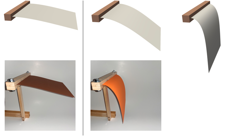
Figure 3. Top row: numerically computed deformed configurations of a plate, clamped on the left side, under a uniform vertical load, with homogeneous material, with Lamé constants scaled with $1.0$ (left), $0.286$ (middle) and $0.02$ (right). Bottom row: photos of physical deformations of paper. Left: thick paper ($300g/m^{2}$) glued on thinner paper ($120g/m^{2}$). Middle: only thin paper ($120g/m^{2}$).

Microstructure with axes aligned stripes. We consider a material distribution with $\gamma=0.1$ that corresponds to a periodic pattern of stripes of alternating hard and soft material aligned with the coordinate directions. On the rescaled microscopic cell $Y\times I$ this corresponds to hard material in the volumes $[\frac{1}{4},\frac{3}{4}]\times[0,1]\times[-\frac{1}{2},\frac{1}{2}]$, and soft material elsewhere. We also take into account the same configuration rotated by $90$ degrees in the $Y$ plane. The constant homogenized tensors $\mathcal{C}^{2,\gamma}$ were computed for a uniformly hexagonal mesh on the unit cube with grid size $h=\tfrac{1}{128}$. The resulting tensors $\mathcal{C}^{2,\gamma}_{||}$ and $\mathcal{C}^{2,\gamma}_{=}$, respectively, written as matrices in Voigt type notation, corresponding to the basis (30) are

$$\mathcal{C}^{2,\gamma,v}_{||}=\begin{pmatrix}0.04265&0.00853&0\\ 0.00853&0.5149&0\\ 0&0&0.05099\end{pmatrix}\,,\quad\mathcal{C}^{2,\gamma,v}_{=}=\begin{pmatrix}0.5149&0.00853&0\\ 0.00853&0.04265&0\\ 0&0&0.05099\end{pmatrix}\,.$$

The plate is clamped on $[0,\frac{1}{5}]\times[\frac{2}{5},\frac{3}{5}]$ and a uniform force $f=(0,0,-5)^{\top}$ is taken into account. In resulting deformations are shown in Figure 4. One observes that the microscopic pattern leads to very stiff behavior of the plate in the direction of the stripes and a very flexible behavior in the perpendicular direction. We compare it with a corresponding paper experiment. To this end, a sheet of paper (green, $120g/m^{2}$) of size $28cm\times 28cm$ is used with stripes of thick paper (red, $300g/m^{2}$) of width $4mm$ where glued on top with a stripe distance of $4mm$. The resulting layered paper is clamped between two pieces of wood (cf. Figure 4).

Microstructure reflecting radially arranged stripes. Under the force and boundary conditions of the above experiment, we next consider a microstructure that mimics radial arranged rays of hard material centered at the midpoint $(0,0.5)$ of the left-hand side of the plate. The width of the stripes is proportional to the distance from the center.

First, we consider a stripe pattern similar to the one considered above with hard material on $(0,1)\times(\tfrac{1}{3},\tfrac{2}{3})\times(-\tfrac{1}{2},\tfrac{1}{2})$ and soft material elsewhere, where the ratio of the hard material $\tfrac{1}{3}$ equals the ratio of the angle of a single hard material stripe and the angle of a single soft material stripe in the radially arranged strip pattern in the corresponding experiment. For a point $x\in\omega$ with $x-(0,0.5)=(r\cos\alpha,r\sin\alpha)$ for $\alpha\in(0,\pi)$ and $r\in\mathbb{R}_{+}$, we consider $\gamma=ar+b$, for $a,b\in\mathbb{R}$, such that $1=\frac{1}{5}a+b$ and $\frac{1}{10}=\frac{\sqrt{5}}{2}a+b$. This models the widening of the strips while maintaining the thickness of the plate. Let us denote the resulting homogenized tensor by $\widehat{\mathcal{C}}^{2,\gamma}$ .

Then, applying the coordinate transformation formula [2, Section 3.4] the resulting homogenized tensor $\mathcal{C}^{2,\gamma}(x)$ reflecting the radially arranged stripe pattern at $x\in\omega$ is given by

$$\mathcal{C}^{2,\gamma}(x)A:A\coloneqq \widehat{\mathcal{C}}^{2,\gamma}A_{\alpha}:A_{\alpha}\textit{ with }A_{\alpha}\coloneqq\begin{pmatrix}\cos\alpha&\sin\alpha\\ -\sin\alpha&\cos\alpha\end{pmatrix}A\begin{pmatrix}\cos\alpha&-\sin\alpha\\ \sin\alpha&\cos\alpha\end{pmatrix}$$

for all $A\in\mathbb{R}^{2\times 2}_{\text{sym}}$.

In Figure 4 in the top right, the resulting deformation is shown. Below, on a $28cm\times 28cm$ sheet of paper (purple, $120g/m^{2}$), we take into account 16 glued on stripes of thicker paper (yellow, $300g/m^{2}$), radially symmetric, broadening with the distance from the clamped center part of the paper. The opening angle of the hard material (yellow) is $3.75^{\circ}$ and the opening angle of the soft material (purple) is $7.5^{\circ}$ with the width of the hard material stripes ranges from $1mm$ to $1.2cm$.

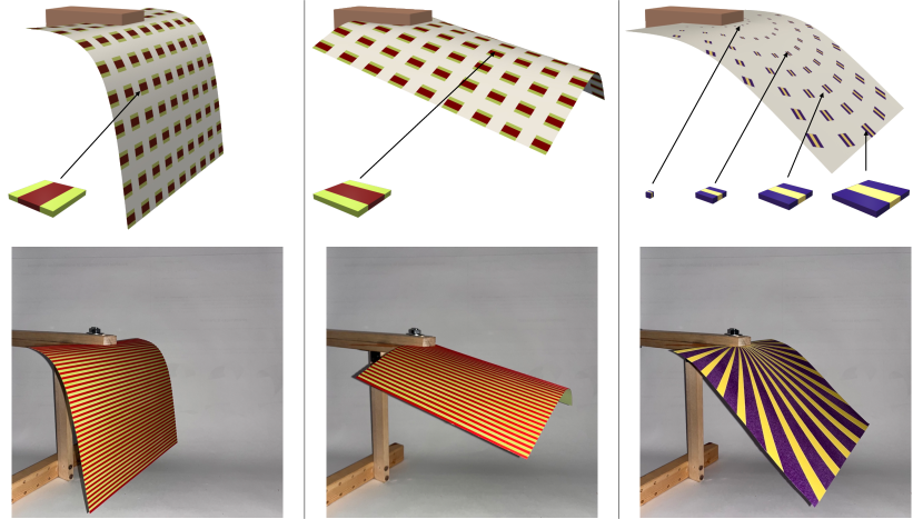
Figure 4. Top row: deformed configurations under a uniform vertical load for stripe-type microstructures (left and middle) and a microstructure with radial rays (right). Bottom row: photos of physical experiments with stripes of thicker paper ($300g/m^{2}$, left and middle: red, right: yellow) glued on thinner paper ($120g/m^{2}$, left and middle: green, right: purple).

Microstructure with periodic diagonal aligned stripe pattern. Now, we consider a constantly distributed microstructure consisting of layers of hard and soft material oriented diagonally in the first two coordinates, i.e.the hard material phase is given by all $y=(y^{\prime},y_{3})$ with

$$\left|y^{\prime}-\begin{pmatrix}1\\ 0\end{pmatrix}\right|_{1}\in(\tfrac{1}{4},\tfrac{3}{4})\cap(\tfrac{5}{4},\tfrac{7}{4})\,$$

where $|\cdot|_{1}$ is the $1$-norm in $\mathbb{R}^{2}$. The resulting homogenized tensor in Voigt-type notation is

$$\mathcal{C}^{2,\gamma,v}=\begin{pmatrix}0.17883&0.10699&0.11725\\ 0.10699&0.17883&0.11725\\ 0.11725&0.11725&0.13436\end{pmatrix}\,.$$

The deformation was enforced by the boundary conditions (33) reflecting a compression in the $x_{1}$ direction by a factor $\tfrac{6}{16}$. No surface load applies. Again, a small random initial deformation is considered. The computed deformation is shown in Figure 5 on the top left. The qualitative behavior is compared with a sheet of paper (blue, $120g/m^{2}$) of size $28cm\times 28cm$, where stripes of thick paper (orange, $300g/m^{2}$) of width $5mm$ were glued on, with a distance of $5mm$, in direction of one diagonal of the paper. A photo of this experiment is shown in 5 on the left of the bottom row. Due to the anisotropic microscopic material distribution the macroscopic elastic energy is also anisotropic leading both in the simulation and the experiment to a firm twist of the resulting valley formed by the bent plate.

Microstructure with axes aligned and diagonal trusses of hard material. In this experiment, we take into account a macroscopically varying microstructure with trusses of hard material on a soft material background. In the rescaled model with vertically homogeneous material on $(0,1)^{2}\times(-\tfrac{1}{2},\tfrac{1}{2})$ the hard material phase is given by

$$\big{\{}y\;:\; 1-\tfrac{b}{\sqrt{2}}|y^{\prime}-(1,0)^{\top}|_{1}<1+\tfrac{b}{\sqrt{2}}\vee 1-\tfrac{b}{\sqrt{2}}|y^{\prime}|_{1}<1+\tfrac{b}{\sqrt{2}}\vee$$

$$y_{1}<\tfrac{a}{2}\vee y_{1}>1-\tfrac{a}{2}\vee y_{2}<\tfrac{a}{2}\vee y_{2}>1-\tfrac{a}{2}\big{\}}$$

with thickness $a(y_{1})=(1-y_{1})\frac{2-\sqrt{3}}{2}$, $b(y_{1})=y_{1}\frac{2-\sqrt{3}}{2}$ of the axes aligned and diagonal trusses, respectively. The prototype of the fundamental cell and the resulting fine scale pattern with cell size $\varepsilon=\tfrac{1}{16}$ in $y^{\prime}$ coordinates is depicted in Figure 5 on the right. On the macroscale the boundary conditions (33) and load are applied. Furthermore, for the paper experiment counterpart, the truss structure with $14^{2}$ $2cm\times 2cm$ cells of thick paper ($300g/m^{2}$) is glued on a $28cm\times 28cm$ thin paper ($120g/m^{2}$). A comparison of the simulated deformation for the homogenized model and the experiment is shown as well in Figure 5. It is clearly visible that the bent plate is no longer symmetric in $x_{1}$ direction and the bending is much stronger on the right.

Figure 5. Top left: deformed configuration under compression enforced by the boundary conditions (33) with soft material in blue and hard material in orange, bottom left: corresponding experiment with stripes of thicker paper ($300g/m^{2}$, orange) glued on thin paper ($120g/m^{2}$blue); top middle: deformed configuration for a truss type microstructure under the same boundary conditions, with soft material in red and hard material in white, top right material distribution on the rescaled microscopic cell, bottom middle: a correspondingly deformed sheet of paper (red) with glued layer structure of the thicker paper (white), bottom right: undeformed experimental plate configuration viewed from above.

References

• [1] G. Allaire, and R. Brizzi, A Multiscale Finite Element Method for Numerical Homogenization, Multiscale Modeling and Simulation, 4 (2005), pp. 790–812.
• [2] G. Allaire, P. Geoffroy-Donders, and O. Pantz, 3-d topology optimization of modulated and oriented periodic microstructures by the homogenization method, Journal of Computational Physics, 401 (2020)
• [3] S. Bartels, Approximation of large bending isometries with discrete Kirchhoff triangles, SIAM J. Numer. Anal., 51 (2013), pp. 516–525.
• [4] S. Bartels, Numerical methods for nonlinear partial differential equations, vol. 47 of Springer Series in Computational Mathematics, Springer, Cham, 2015.
• [5] S. Bartels, Numerical solution of a Föppl–von Kármán model, SIAM Journal on Numerical Analysis, 55 (2017), pp. 1505–1524.
• [6] S. Bartels, A. Bonito, and R. H. Nochetto, Bilayer plates: Model reduction, $\Gamma$-convergent finite element approximation, and discrete gradient flow, Communications on Pure and Applied Mathematics, 70 (2017), pp. 547–589.
• [7] K. Böhnlein, S. Neukamm, D. Padilla-Garza, and O. Sander, A Homogenized Bending Theory for Prestrained Plates, Journal of Nonlinear Science, 33 (2023).
• [8] A. Bonito, D. Guignard, R. Nochetto, and S. Yang, Numerical analysis of the LDG method for large deformations of prestrained plates, arXiv preprint arXiv:2106.13877, (2021).
• [9] A. Bonito, R. H. Nochetto, and D. Ntogkas, DG approach to large bending plate deformations with isometry constraint, (2020).
• [10] D. Braess, Finite Elements, Springer, 5 ed., 2013.
• [11] P.G. Ciarlet, The finite element method for elliptic problems, North-Holland Publishing Co., Amsterdam-New York-Oxford, (1978).
• [12] M. de Benito Delgado, and B. Schmidt, A hierarchy of multilayered plate models, ESAIM: Control, Optimisation and Calculus of Variations, 27 (2021).
• [13] W. E, B. Engquist, and Z. Huang, Heterogeneous Multiscale Method: A General Methodology for Multiscale Modeling, Physical Review B, 67 (2003).
• [14] W. E, P. Ming, and P. Zhang, Analysis of the heterogeneous multiscale method for elliptic homogenizationproblems, J. Amer. Math. Soc., 18 (2005).
• [15] G. Friesecke, R. D. James, and S. Müller, A theorem on geometric rigidity and the derivation of nonlinear plate theory from three-dimensional elasticity, Comm. Pure Appl. Math., 55 (2002), pp. 1461–1506.
• [16] D. Gilbarg, and N.S. Trudinger, Elliptic partial differential equations of second order, Springer-Verlag, Berlin, (1992).
• [17] P. Hornung, Approximation of flat $W^{2,2}$ isometric immersions by smooth ones, Arch. Ration. Mech. Anal., 199 (2011), pp. 1015–1067.
• [18] P. Hornung, Stationary points of nonlinear plate theories, Journal of Functional Analysis, 273 (2017), pp.946–983.
• [19] P. Hornung, S. Neukamm, and I. Velčić, Derivation of a homogenized nonlinear plate theory from 3d elasticity, Calculus of variations and partial differential equations, 51 (2014), pp. 677–699.
• [20] S. Neukamm, and H. Olbermann, Homogenization of the nonlinear bending theory for plates, Calculus of Variations and Partial Differential Equations, 53 (2015), pp. 719–753.
• [21] M. Rumpf, S. Simon, and C. Smoch, Finite Element Approximation of Large-Scale Isometric Deformations of Parametrized Surfaces, SIAM Journal on Numerical Analysis, 60 (2022), pp. 2945–2962.
• [22] I. Velčić, On the derivation of homogenized bending plate model, Calculus of variations and partial differential equations, 53 (2015), pp. 561–586.
• [23] A. Wächter and L. T. Biegler, On the Implementation of a Primal-Dual Interior Point Filter Line Search Algorithm for Large-Scale Nonlinear Programming, Mathematical Programming, 106 (2006), pp. 25–57.
• [24] T. Yokoyama, and K. Nakai, Evaluation of in-plane orthotropic elastic constants of paper and paperboard, Proceeding of 2007 SEM Annual Conference & Exposition on Experimental and Applied Mechanics, (2007).