Task-Aware Machine Unlearning and Its Application in Load Forecasting

Abstract

Data privacy and security have become a non-negligible factor in load forecasting. Previous researches mainly focus on training stage enhancement. However, once the model is trained and deployed, it may need to ‘forget’ (i.e., remove the impact of) part of training data if the data is found to be malicious or as requested by the data owner. This paper introduces machine unlearning algorithm which is specifically designed to remove the influence of part of the original dataset on an already trained forecaster. However, direct unlearning inevitably degrades the model generalization ability. To balance between unlearning completeness and performance degradation, a performance-aware algorithm is proposed by evaluating the sensitivity of local model parameter change using influence function and sample re-weighting. Moreover, we observe that the statistic criterion cannot fully reflect the operation cost of down-stream tasks. Therefore, a task-aware machine unlearning is proposed whose objective is a tri-level optimization with dispatch and redispatch problems considered. We theoretically prove the existence of the gradient of such objective, which is key to re-weighting the remaining samples. We test the unlearning algorithms on linear and neural network load forecasters with realistic load dataset. The simulation demonstrates the balance on unlearning completeness and operational cost. All codes can be found at https://github.com/xuwkk/task_aware_machine_unlearning.

I Introduction

I-A Data Privacy and Security in Load Forecasting

Accurate load forecasting is essential to secure and economic power system operations. Deterministic [1] and probabilistic [2] methods are two main categories. Recently, machine and deep learning algorithms have been widely applied to better retrieve the spatial and temporal information, which certainly benefit the progression of load forecasting [3]. To fulfill the training purpose, large amount of data from diverse sources is collected, which challenges the integrity of data ownership and security.

Conventionally, the system operator (SO) collects and transfers the individual data for various operational purpose. However, this arrangement has raised concerns as individual load data is sensitive and can be targeted for retrieving personal identity and behaviour [4]. From the perspective of data security, data collections are prone to errors and adversaries. For instance, authors in [5] benchmarks how the poor training data could degrade the forecasting accuracy by introducing random noises. Moreover, data poisoning attack is specifically designed to contaminate the training dataset to mislead the load forecaster from being accurate at the test stage [6].

Most of the existing work designs preventive training algorithm to tackle the concerns in data privacy and security. For instance, federated learning is studied, in which each training participant only shares the trained parameters to the central server [7]. A fully distributed training framework has been proposed in [8] where each participant only share the parameters with their neighbours. Differential privacy is another privacy-preserving technique used for load forecasting to avoid spotting on individual’s identity [9]. To tackle the poisoning attack, differential privacy-enhanced federated learning is developed in [10]. By weight clipping and adding noise to the central parameter update, the global model can be resistant to inference attack to some extent. In addition, gradient quantization is applied in [11] where each participant only uploads the sign of the local gradient.

I-B Machine Unlearning

However, training stage prevention is not sufficient and there are situations where a post-action of removing the impact of those data from the trained forecaster is needed. From the privacy concerns, in addition to the right to share the data, many national and regional regulations have certified the consumers’ ‘right to forget’ [12], such as European Union’s General Data Protection Regulation (GDPR) and the recent US’s California Consumer Privacy Act (CCPA). I.e., the consumers are eligible to ask to destroy their personal records at any stage of the service including the encoded information in the trained model. In the meantime, SO may not be aware of the data defect until the model is already trained and deployed. Obviously, one straight approach is retraining the model from scratch on the remaining data. However, retraining can be computationally expensive and an ideal method is to use the already-trained model as a starting point.

In this context, machine unlearning (MU) is recently introduced in machine learning community to study the problem of removing a subset of training data, the forget set, from the trained model. Although retraining is not a viable option, it is usually assumed that the golden rule for unlearning is to minimize the distance between the unlearnt and the retrained models in literature [13]. Particularly, the gradient and the Hessian matrix of the training objective are utilized for approximating the influence of the samples on the trained model parameters, such as Fisher information [14] and influence function [15]. Motivated from differential privacy, [16] certifies the the exactness of data removal on linear classifiers. However, the approximate method is hard to generalize to neural network (NN) [17]. A mixed-privacy forgetting is proposed to only unlearn on a linear regressor upon the trained NN [15, 16]. More information on machine unlearning can be found in the recent review [13].

I-C Research Gaps

I-C1 Unlearning Completeness vs Performance Degradation

The golden rule of unlearning may not be suitable for real-world applications. Referring to Table I, when the privacy is mainly concerned (privacy-driven MU), although the golden rule can certainly remove the influence of the forget dataset, it can inevitably degrade the performance of the trained model so that the interest of the remaining customers are harmed [18]. As for the security-driven MU, the maclicious data can still contain useful information. However, the golden rule not only removes the adverse influence of the forget dataset but also the useful one.

Table I: The Purposes of Unlearning

MU Purpose	Description	Target
Privacy-driven	Some training data contains sensitive information and is asked to remove by the customer.	The main target is to unlearn the model as if it is originally trained without the forget data.
Security-driven	Some training data is malicious, whose influence should be removed from the trained model by the system operator.	The main target is to remove the malicious information from the model while keeping the useful information.

We argue that there exists a trade-off between the unlearning completeness and the performance degradation. In detail, the unlearning completeness is defined as the mismatch between the unlearnt model to the retrained model, which can be evaluated by the distance between the parameters, or the accuracy on the train and test dataset, i.e. the golden rule of unlearning. The performance degradation represents how the generalization ability of the unlearnt model degrades based on certain criterion. How to quantitatively calculate the two factors effectively and efficiently without knowing the retrained model, needs to be investigated.

I-C2 Physical Meaning of Power System

Apart from the completeness and performance trade-off, directly applying the MU algorithms from machine learning community overlooks the physical meaning of power system. In load forecasting, the ultimate goal is to use the forecast load for the downstream tasks, such as dispatching the generator. As shown by [19, 20], the forecast error mismatches the deviation of generator cost such that a highly accurate load forecaster may not result in economic power system operation. Intuitively, we argue that the performance of MU also deviated from accuracy criterion to the task-aware generator cost. Therefore, the cost of generator needs to be evaluated as the performance criterion when dealing with the completeness-performance trade-off.

I-D Contributions

The contributions of this paper are summarized as follows:

• Machine Unlearning: As far as we know, this is the first paper applying machine unlearning to power system applications. Specifically, we introduce machine unlearning to load forecasting model (shown by Fig.1). The influence of forget dataset on the trained model is evaluated by influence function based approach, which is eliminated by Newton’s update. Such unlearning algorithm is complete on linear load forecaster.

• Completeness-Performance Trade-off: We show that unlearning can inevitably cause the statistic performance degradation, such as drops in mean squared error (MSE) and mean absolute percentage error (MAPE). To balance the trade-off, the influence function is used to quantify the impact on the statistic performance of each sample, which allows to re-weight the remaining dataset through optimization and improve the performance through performance-aware machine unlearning (PAMU).

• Task-aware Machine Unlearning: At last, we demonstrate that the statistic performance cannot reflect the ultimate goal in power system, such as minimizing the cost of generator dispatch. Therefore, a task-aware machine unlearning (TAMU) is proposed by formulating the unlearning objective as a tri-level optimization. We theoretically prove the existence of the gradient of such task-aware objective, which is key to sample re-weighting.

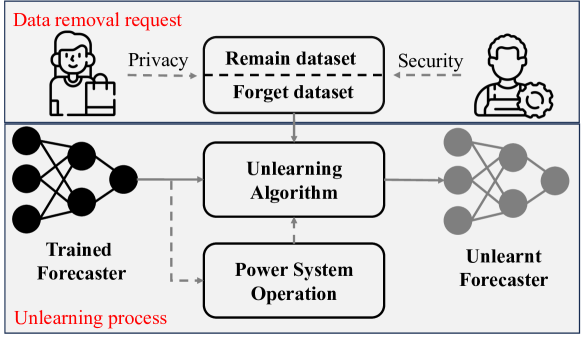
Figure 1: A workflow of machine unlearning. The data removal request can be made by privacy and security concerns. An unlearning algorithm is developed to update the forecaster with the role of power system operation being considered.

II Machine Unlearning for Load Forecasting

II-A Parametric Load Forecasting Model

In this paper, we consider load forecasting problem with $n$ loads/participants. Given dataset $\mathcal{D}=\{(\bm{x}^{i},\bm{y}^{i})\}_{i=1}^{N}$. Let $\bm{x}^{i}\in\mathbb{R}^{n\times M}$ be the feature matrix, e.g. each load has feature of length $M$, and $\bm{y}^{i}\in\mathbb{R}^{n}$ be the ground-truth load. A parametric model $\bm{f}(\cdot;\bm{\theta}):\mathbb{R}^{n\times M}\times\mathbb{R}^{P}\rightarrow\mathbb{R}^{n}$ can be trained by

$$\bm{\theta}^{\star}=\arg\min_{\bm{\theta}}\mathcal{L}(\bm{\theta})=\arg\min_{\bm{\theta}}\frac{1}{N}\sum_{i=1}^{N}\ell(\bm{f}(\bm{x}^{i};\bm{\theta}),\bm{y}^{i})$$ (1)

where $\mathcal{L}(\bm{\theta})$ is the training loss. For simplicity, denote $\ell(\bm{f}(\bm{x}^{i};\bm{\theta}),\bm{y}^{i})$ as $\ell^{i}(\bm{\theta})$ as the loss on the $i$-th sample. MSE is commonly used as the training loss by assuming the forecast error follows Gaussian distribution, i.e., $\ell^{i}(\bm{\theta})=\|\bm{f}(\bm{x}^{i};\bm{\theta})-\bm{y}^{i}\|^{2}_{2}$.

In addition to the training dataset $\mathcal{D}$, there is a test dataset $\mathcal{D}_{\text{test}}$ on which a test criterion can be performed:

$$\mathcal{L}_{\text{test}}(\bm{\theta}^{\star})=\frac{1}{N_{\text{test}}}\sum_{i=1}^{N_{\text{test}}}\ell_{\text{test}}^{i}(\bm{\theta}^{\star})$$ (2)

The test criterion $\ell_{\text{test}}^{i}(\bm{\theta})$ can be different to the training loss $\ell^{i}(\bm{\theta})$. For instance, the load forecasting model can be trained with MSE loss, but is usually evaluated by MAPE, etc. In this paper, we call the loss/criterion such as MSE and MAPE as statistic(-driven) loss/criterion.

II-B Influence Function

Influence function defines a second-order method to evaluate the parameter changes when training samples are up-weighted by a small amount [21]. Define a sub-dataset $\mathcal{D}_{\text{up}}\subseteq\mathcal{D}$. For every sample $j\in\mathcal{D}_{\text{up}}$ up-weighted by $\epsilon^{j}$, the new objective function can be written as

$$\bm{\theta}_{\text{mod}}^{\star} =\arg\min_{\bm{\theta}}\mathcal{L}_{\text{mod}}(\bm{\theta})$$ (3)

$$=\arg\min_{\bm{\theta}}\underbrace{\frac{1}{N}\sum_{i\in\mathcal{D}}\ell^{i}(\bm{\theta})}_{\mathcal{L}(\bm{\theta})}+\underbrace{\frac{1}{N}\sum_{j\in\mathcal{D}_{\text{up}}}\epsilon^{j}\ell^{j}(\bm{\theta})}_{\mathcal{L}_{\text{up}}(\bm{\theta})}$$

The first-order optimality condition gives that

$$\nabla\mathcal{L}_{\text{mod}}(\bm{\theta}_{\text{mod}}^{\star})=0$$ (4)

Apply the first-order Taylor expansion around $\bm{\theta}^{\star}$ on (4):

$$\nabla\mathcal{L}_{\text{mod}}(\bm{\theta}^{\star})+\nabla^{2}\mathcal{L}_{\text{mod}}(\bm{\theta}^{\star})(\bm{\theta}_{\text{mod}}^{\star}-\bm{\theta}^{\star})\cong 0$$

Consequently, up-weighting samples in $\mathcal{D}_{\text{up}}$ can approximately result in parameter changes

$$\bm{\theta}_{\text{mod}}^{\star}-\bm{\theta}^{\star}\cong-\left(\nabla^{2}\mathcal{L}_{\text{mod}}(\bm{\theta}^{\star})\right)^{-1}\nabla\mathcal{L}_{\text{mod}}(\bm{\theta}^{\star})$$ (5)

Furthermore, since $\nabla\mathcal{L}(\bm{\theta}^{\star})=0$, $\nabla\mathcal{L}_{\text{mod}}(\bm{\theta}^{\star})=\nabla\mathcal{L}_{\text{up}}(\bm{\theta}^{\star})$. Eq. (5) can be rewritten as

$$\bm{\theta}_{\text{mod}}^{\star}-\bm{\theta}^{\star}\cong-\left(\nabla^{2}\mathcal{L}_{\text{mod}}(\bm{\theta}^{\star})\right)^{-1}\nabla\mathcal{L}_{\text{up}}(\bm{\theta}^{\star})$$ (6)

When $\epsilon_{j}$ is small and/or $|\mathcal{D}_{\text{up}}|\ll|\mathcal{D}|$, $\nabla^{2}\mathcal{L}_{\text{mod}}(\bm{\theta}^{\star})\cong\nabla^{2}\mathcal{L}(\bm{\theta}^{\star})$. Therefore, (6) is further approximated as

$$\bm{\theta}_{\text{mod}}^{\star}-\bm{\theta}^{\star}\cong-\left(\nabla^{2}\mathcal{L}(\bm{\theta}^{\star})\right)^{-1}\nabla\mathcal{L}_{\text{up}}(\bm{\theta}^{\star})$$ (7)

where $\nabla\mathcal{L}_{\text{up}}(\bm{\theta}^{\star})=\frac{1}{N}\sum_{j\in\mathcal{D}_{\text{up}}}\epsilon^{j}\nabla\ell^{j}(\bm{\theta}^{\star})$ and $\nabla^{2}\mathcal{L}(\bm{\theta}^{\star})=\frac{1}{N}\sum_{j\in\mathcal{D}}\nabla^{2}\ell^{j}(\bm{\theta}^{\star})$.

We highlight that (5)-(7) are Newton’s update on the parameter with respect to the new objective (3). Therefore, for multi-variate linear load forecaster with MSE loss, (5) and (6) are exact update on the trained model $\bm{\theta}^{\star}$.

II-C Machine Unlearning Algorithm

From data privacy perspective, participants are eligible to ask the SO to remove their data and eliminate any influence on the trained model $\bm{\theta}^{\star}$. When a request on record $j$ happens, the corresponding datum $(\bm{x}^{j},\bm{y}^{j})$ needs to be removed from the training dataset. In the meantime, $\mathcal{D}$ may contain erroneous or malicious data, caused by rough data collection or poisoning attack, whose influence on the trained forecaster needs to be removed after the model is trained.

Define $\mathcal{D}_{\text{unlearn}}\subset\mathcal{D}$ be the dataset that needs to be removed and $|\mathcal{D}_{\text{unlearn}}|\ll|\mathcal{D}|$. A trivial solution to unlearn the data is to retrain the model on the remaining dataset $\mathcal{D}_{\text{remain}}=\mathcal{D}\setminus\mathcal{D}_{\text{unlearn}}$ from scratch. When retraining is not viable due to the data availability and urgency of the request, a commonly used MU algorithm can be directly derived from influence function by setting $\epsilon_{j}=-1$ in (3). As a result, (5) can be modified as

$$\bm{\theta}_{\text{remain}}^{\star}\cong\bm{\theta}^{\star}-\left(\sum_{i\in\mathcal{D}_{\text{remain}}}\nabla^{2}\ell^{i}(\bm{\theta}^{\star})\right)^{-1}\sum_{i\in\mathcal{D}_{\text{remain}}}\nabla\ell^{i}(\bm{\theta}^{\star})\\$$ (8)

For a linear forecaster, unlearning (8) is complete, satisfying the golden rule of unlearning. Similar unlearning algorithms can also be derived from (6) and (7).

III Performance-aware Machine Unlearning

A complete MU algorithm on linear load forecaster such as (8) can inevitably degrade the performance on the test dataset (will be shown in the simulation). Followed by the previous work in [18], a performance-aware machine unlearning (PAMU) is derived by re-weighting the remaining samples based on their distinct contribution to the statistic criterion (2).

The influence function (7) can be further extended to evaluate the test set performance change due to the up-weighted objective (3) [17, 22, 18]. To start, the performance on the test dataset for model parameterized by $\bm{\theta}^{\star}_{\text{remain}}$ can be written as

$$\mathcal{L}_{\text{test}}(\bm{\theta}^{\star}_{\text{remain}})=\frac{1}{N_{\text{test}}}\sum_{i=1}^{N_{\text{test}}}\ell_{\text{test}}^{i}(\bm{\theta}_{\text{remain}}^{\star})$$ (9)

Applying first-order Taylor expansion on (9) gives:

$$\mathcal{L}_{\text{test}}(\bm{\theta}^{\star}_{\text{remain}})$$ (10)

$$\cong \underbrace{\frac{1}{N_{\text{test}}}\sum_{i=1}^{N_{\text{test}}}\ell_{\text{test}}^{i}(\bm{\theta}^{\star})}_{\mathcal{L}_{\text{test}}(\bm{\theta}^{\star})}+\frac{1}{N_{\text{test}}}\sum_{i=1}^{N_{\text{test}}}\nabla\ell_{\text{test}}^{i}(\bm{\theta}^{\star})^{T}(\bm{\theta}_{\text{remain}}^{\star}-\bm{\theta}^{\star})$$

To balance the performance degradation, the remaining dataset can be re-weighted. The idea is straight-forwardly that, after unlearning, different remaining samples will be affected distinctly which needs to be re-weighted as if they are being re-trained.

The new objective function on the re-weighted remaining dataset can be written as

$$\bm{\theta}_{\text{remain},\epsilon}^{\star}=\arg\min_{\bm{\theta}}\frac{1}{N}\sum_{i\in\mathcal{D}_{\text{remain}}}\epsilon_{i}\ell^{i}(\bm{\theta})$$ (11)

where $\epsilon_{i}$ is an unknown weight for sample $i$ in the remaining dataset. Referring to (5), the parameter changes can be approximated as

$$\bm{\theta}_{\text{remain},\epsilon}^{\star}-\bm{\theta}^{\star}\cong-\left(\sum_{i\in\mathcal{D}_{\text{remain}}}\epsilon_{i}\nabla^{2}\ell^{i}(\bm{\theta}^{\star})\right)^{-1}\sum_{i\in\mathcal{D}_{\text{remain}}}\epsilon_{i}\nabla\ell^{i}(\bm{\theta}^{\star})$$ (12)

Plugging (12) into (10), the performance changes can be written as:

$$\mathcal{L}_{\text{test}}(\bm{\theta}^{\star}_{\text{remain},\epsilon})-\mathcal{L}_{\text{test}}(\bm{\theta}^{\star})\cong\bm{m}^{T}\sum_{i\in\mathcal{D}_{\text{remain}}}\epsilon_{i}\nabla\ell^{i}(\bm{\theta}^{\star})$$ (13)

where

$$\bm{m}^{T}=-\frac{1}{N_{\text{test}}}\sum_{i\in\mathcal{D}_{\text{test}}}\nabla\ell_{\text{test}}^{i}(\bm{\theta}^{\star})^{T}\left(\sum_{i\in\mathcal{D}_{\text{remain}}}\epsilon_{i}\nabla^{2}\ell^{i}(\bm{\theta}^{\star})\right)^{-1}$$ (14)

When $\epsilon_{i}$ is close to 1, the $\bm{m}$ vector can be approximated as

$$\tilde{\bm{m}}^{T}=-\frac{1}{N_{\text{test}}}\sum_{i\in\mathcal{D}_{\text{test}}}\nabla\ell_{\text{test}}^{i}(\bm{\theta}^{\star})^{T}\left(\sum_{i\in\mathcal{D}_{\text{remain}}}\nabla^{2}\ell^{i}(\bm{\theta}^{\star})\right)^{-1}$$ (15)

Our goal is to find an optimal weights to improve the test set performance, which can be formulated as a constrained optimization problem:

$$\bm{\epsilon}^{\star}= \arg\min_{\bm{\epsilon}}\tilde{\bm{m}}^{T}\sum_{i\in\mathcal{D}_{\text{remain}}}\epsilon_{i}\nabla\ell^{i}(\bm{\theta}^{\star})$$ (16)

$$\text{s.t.}\quad\quad\quad\frac{1}{N_{\text{remain}}}\|\bm{\epsilon}-\bm{1}\|_{1}\leq\lambda_{1},\quad\|\bm{\epsilon}-\bm{1}\|_{\infty}\leq\lambda_{\infty}$$

where $\bm{\epsilon}\in\mathbb{R}^{|\mathcal{D}_{\text{remain}}|}$ and $\bm{1}\in\mathbb{R}^{|\mathcal{D}_{\text{remain}}|}$.

In (16), the weight of the remaining samples are optimized so that the influence of forgetting $\mathcal{D}_{\text{unlearn}}$ is reduced. Since the first-order Taylor expansion (10) is a local approximation, 1-norm and inf-norm constraints are added to control the aggregated and individual re-weighting. When $\lambda_{1}\rightarrow 0$ or $\lambda_{\infty}\rightarrow 0$, $\bm{\epsilon}\rightarrow 1$, representing the complete machine unlearning (8). When $\lambda_{1}$ and $\lambda_{\infty}$ become larger, the performance on the test dataset improves while the completeness of unlearning is reduced. Therefore, by controlling $\lambda_{1}$ and $\lambda_{\infty}$, the trade-off between the MU completeness and performance degradation can be balanced.

Moreover, compared with [18], the objective of (16) does not take the absolute value. Therefore, it is allowed to improve the performance beyond the originally trained model. Therefore, any uncovered defect data in the remaining dataset will be assigned with a smaller weight and the unlearning becomes an one-step continual learning on the re-weighted samples.

Since both $\tilde{\bm{m}}$ and $\nabla\ell^{i}(\bm{\theta})^{\star},i\in\mathcal{D}_{\text{remain}}$ are calculated in advance, (16) is a convex optimization problem which can be easily solved. Once the optimal weights $\bm{\epsilon}^{\star}$ is optimized, we can unlearn the $\mathcal{D}_{\text{unlearn}}$ through (12). Regarding on different choices of $\ell_{\text{test}}$, e.g. MSE and MAPE, the remaining dataset can be re-weighted in distinct manners. It is also possible to balance different criteria integratedly.

IV Task-aware Machine Unlearning

IV-A Formulation and Algorithm

In power systems, the forecast load is further used to schedule generators and the statistic accuracy of the forecast load is eventually converted into the deviation of the generator cost, which is strongly linked to the value of each sample as well as the profit of the SO and participants. As a result, PAMU guided by the statistic-driven criterion may not reflect on the ultimate goal of power system operation, and a further step on PAMU is needed to balance the generator cost, which can be done by taking the generator cost as the new test criterion.

To measure the impact of model parameter $\bm{\theta}$ on the objective (18), the following task-aware criterion $\mathcal{L}_{\text{gen}}(\bm{\theta})$ can be formulated:

$$\min_{\bm{\theta}}\frac{1}{N_{\text{test}}}\sum_{i=1}^{N_{\text{test}}}\ell_{\text{gen}}^{i}(\bm{\theta})$$ (17)

s.t. $$\left\{\begin{array}[]{l}\text{(Re-dispatch):}\\ (\bm{P}_{ls}^{i\star},\bm{P}_{gs}^{i\star})\in\arg\min\{c_{ls2}\|\bm{P}_{ls}^{i}\|_{2}^{2}+c_{gs2}\|\bm{P}_{gs}^{i}\|_{2}^{2}\\ \qquad\qquad\qquad\qquad+c_{ls}\|\bm{P}_{ls}^{i}\|_{1}+c_{gs}\|\bm{P}_{gs}^{i}\|_{1}:\\ \qquad\qquad\qquad\qquad(\bm{P}_{ls}^{i},\bm{P}_{gs}^{i})\in\mathcal{C}_{\text{redispatch}}(\bm{P}_{g}^{i\star},\bm{y}^{i})\}\\ \text{(Dispatch):}\\ \bm{P}_{g}^{i\star}\in\arg\min\{\bm{P}_{g}^{iT}\bm{Q}_{g}\bm{P}_{g}^{i}+\bm{c}_{g}^{T}\bm{P}_{g}^{i}+c_{ls}\|\bm{s}^{i}\|_{1}:\\ \qquad\qquad\qquad\qquad\bm{P}_{g}^{i}\in\mathcal{C}_{\text{dispatch}}(\hat{\bm{y}}^{i})\}\\ \hat{\bm{y}}^{i}=\bm{f}(\bm{x}^{i};\bm{\theta})\end{array}\right.$$

$$\quad\text{for all }i=1,\cdots,|\mathcal{D}_{\text{test}}|$$

Task-aware criterion (17) can be viewed as a tri-level optimization problem with two lower levels, taking the expectation over the test dataset. For each sample, lower level one is a dispatch problem that minimizes the generator cost subject to system operation constraint $\mathcal{C}_{\text{dispatch}}$. $\bm{P}_{g}$ is the generator dispatch. Lower level two is a re-dispatch problem which aims to balance any under- or over-generation due to inaccurate forecast though load shedding $\bm{P}_{ls}$ and generation storage $\bm{P}_{gs}$, under the constraint set $\mathcal{C}_{\text{redispatch}}$. The upper level, which represents the expected operation cost, can be determined as the integration of the two stages:

$$\begin{array}[]{rl}&\ell_{\text{gen}}(\bm{P}_{g},\bm{P}_{ls},\bm{P}_{gs};\bm{\theta})\\ =&\bm{P}_{g}^{T}\bm{Q}_{g}\bm{P}_{g}+c_{ls2}\|\bm{P}_{ls}\|_{2}^{2}+c_{gs2}\|\bm{P}_{gs}\|_{2}^{2}\\ &+\bm{c}_{g}^{T}\bm{P}_{g}+c_{ls1}\|\bm{P}_{ls}\|_{1}+c_{gs1}\|\bm{P}_{gs}\|_{1}\end{array}$$ (18)

The detailed formulations can be found in Appendix -A. When $\bm{\theta}$ is fixed and if each lower-level problem has unique optimum, (17) is the expected real-time power system operation on the test dataset.

Referring to (10), PAMU needs to calculate the gradient $\nabla\ell^{i}_{\text{gen}}(\bm{\theta}^{\star})$, which seems to be troublesome due to the nested structure and constraints in (17). To solve the problem, firstly for each sample $i$, it can be observed that the lower-level problems are sequentially connected, i.e., the input to the stage-one problem is the forecast load while the input to the stage-two problem is the generator dispatch status from stage-one. Secondly, the lower level problems are also independent among samples and the constraints. Therefore, the lower level optimizations can be viewed as composite function for each sample. Let $\bm{P}_{g}^{i}=\bm{p}^{\star}_{1}(\hat{\bm{y}}^{i})$ and $\bm{P}_{ls,gs}^{i}=\bm{p}^{\star}_{2}(\bm{P}_{g}^{i},\bm{y}^{i})$ be the optimal solution map for dispatch and redispatch, the individual generator cost (18) can be written as a composite function:

$$\ell_{\text{gen}}^{i}(\bm{\theta}^{\star})=\ell_{\text{gen}}^{i}(\bm{p}^{\star}_{1}(\hat{\bm{y}}^{i}),\bm{p}^{\star}_{2}(p^{\star}_{1}(\hat{\bm{y}}^{i}),\bm{y}^{i}))$$ (19)

Alternatively, we can view the lower level optimizations as sequential layers upon the parametric forecasting model. The layer, which represents a constrained optimization problem, is named as differentiable convex layer [23].

Consequently, the TAMU can be achieved by replacing the statistic metric $\ell_{\text{test}}^{i}(\bm{\theta}^{\star})$ by $\ell_{\text{gen}}^{i}(\bm{\theta}^{\star})$, followed by finding the weights of remaining dataset (16) and updating the parameters by (12).

The last issue needs to be resolved is to calculate the gradient of (19) as required by (10). From the chain rule, the gradient of (19) can be written as:

$$\quad\frac{\partial\ell^{i}_{\text{gen}}(\bm{\theta}^{\star})}{\partial\bm{\theta}}$$ (20)

$$= \left(\frac{\partial\ell^{i}_{\text{gen}}(\bm{P}_{g}^{i},\bm{P}_{ls,gs}^{i})}{\partial\bm{P}_{g}}+\frac{\partial\ell^{i}_{\text{gen}}(\bm{P}_{g}^{i},\bm{P}_{ls,gs}^{i})}{\partial\bm{P}_{ls,gs}}\frac{\partial p_{2}^{\star}(\bm{P_{g}}^{i})}{\partial\bm{P}_{g}}\right)$$

$$\quad\times\frac{\partial p_{1}^{\star}(\hat{\bm{y}}^{i})}{\partial\hat{\bm{y}}}\frac{\partial\bm{f}(\bm{\theta}^{\star})}{\partial\bm{\theta}}$$

The gradient flow is highlighted in Fig.2. Based on (20), the gradient $\partial\ell^{i}_{\text{gen}}(\bm{\theta}^{\star})/\partial\bm{\theta}$ exists if the gradient through the differentiable convex layers, namely $\partial p_{1}^{\star}(\hat{\bm{y}}^{i})/\partial\hat{\bm{y}}$ and $\partial p_{2}^{\star}(\bm{P_{g}}^{i})/\partial\bm{P}_{g}$, exist, which is fulfilled under some minor assumptions in the following proposition.

Proposition 1.

The gradients $\partial p_{1}^{\star}(\hat{\bm{y}}^{i})/\partial\hat{\bm{y}}$ and $\partial p_{2}^{\star}(\bm{P_{g}}^{i})/\partial\bm{P}_{g}$ exist, which do not dependent on $\hat{\bm{y}}^{i}$ and $\bm{P_{g}}^{i}$, respectively, if 1). $\bm{Q}$ is positive definite, $\bm{c}_{ls2}$ and $\bm{c}_{gs2}$ are positive; and 2). the linear independent constraint qualification (LICQ) is satisfied at the optimum of each of the lower-level problems.

The proof can be found in Appendix -B.

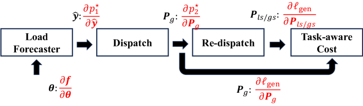
Figure 2: The structure of tri-level optimization (17) viewed as layers in the forward pass. The gradients used in (20) are highlighted in red.

IV-B Extension to Neural Network based Load Forecaster

Unlearning algorithm (8) is complete on the linear load forecaster as the training objective is quadratic. However, the loss function is usually not strongly convex in neural network. In the meantime, its Hessian can be singular due to early stop during the training. This makes the influence function performs poorly to approximate the parameter and performance changes [17] and it becomes harder to evaluate the trade-off between unlearning completeness and performance degradation in PAMU and TAMU.

To tackle the problem, we first divide the training dataset into core and user-sensitive data as $\mathcal{D}_{\text{core}}$ and $\mathcal{D}_{\text{sen}}$, respectively with $\mathcal{D}_{\text{core}}\cap\mathcal{D}_{\text{sen}}=\emptyset$. The core data is assumed to be collected neutrally which does not violate any participant’s privacy and error-free, while the user-sensitive data may be not. Inspired by the transfer learning [24], we first train a load forecaster on the core data $\mathcal{D}_{\text{core}}$ using regular stochastic gradient descent (SGD) and the trained model (except the last layer) can be used as a deep feature extractor.

As illustrated by Fig.3, a feature extractor which excludes the last layer in the load forecaster, is denoted as $\bm{f}(\cdot;\bm{\theta}^{\star}_{\text{FE}})$. Note that Linear Layer 1 includes the activation function on its output. $\mathcal{D}_{\text{sen}}$ is further used to fine tune Linear Layer 2 by the MSE loss. Since using a stochastic gradient method can introduce uncertainties, we propose to fine tune the last layer analytically on $\mathcal{D}_{\text{sen}}$ according to the following proposition.

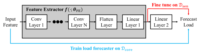
Figure 3: Structure of NN based load forecaster and feature extractor. All the layers except for the Flatten Layer and the Linear Layer 2 contain activations.

Proposition 2.

The optimization problem of minimising the MSE loss on a linear layer without activations is quadratic and has unique minimizer if the the extracted features are linearly independent.

The proof can be found in Appendix -C. To have unique minimizer of Linear Layer 2, we use tanh activation after Linear Layer 1 to avoid trivial outputs of ReLU activation. When an unlearning is requested, the same unlearning algorithms developed previousely can be applied on Linear Layer 2 alone and MU (8) is complete according to Proposition 2. Since the feature extractor only trains on the core data, it does not contain any sensitive information that needs to be unlearnt.

IV-C Computations

We discuss some computational issues and some useful open-source packages in this section.

IV-C1 Inversion of Hessian

Machine unlearning (8) and calculation of vector $\tilde{\bm{m}}$ in PAMU and TAMU require matrix inversion of the Hessian matrix. In general, second order differentiation on the training loss is time-consuming as storing and inverting Hessian matrix requires $\mathcal{O}(d^{3})$ operations where $d$ represents the number of parameter in the load forecast model.

Using $\tilde{\bm{m}}$ (15) as a example:

$$\tilde{\bm{m}}^{T}=\underbrace{-\frac{1}{N_{\text{test}}}\sum_{i=1}^{N_{\text{test}}}\nabla\ell_{\text{test}}^{i}(\bm{\theta}^{\star})^{T}}_{\bm{v}^{T}\in\mathbb{R}^{1\times d}}\underbrace{\left(\sum_{i\in\mathcal{D}_{\text{remain}}}\nabla^{2}\ell^{i}(\bm{\theta}^{\star})\right)^{-1}}_{\bm{H}^{-1}\in\mathbb{R}^{d\times d}}$$ (21)

Calculating $\tilde{\bm{m}}$ can be reduced to solve a linear system:

$$\bm{H}\cdot\bm{m}=\bm{v}$$ (22)

Conjugate gradient (CG) descent algorithm can be applied to solve (22) upto $d$ iterations. We also apply Hessian-Vector Product (HVP) [25] to directly calculate $\bm{H}\bm{m}^{k}$ for the $k$-th iteration in CG so that the Hessian matrix will never be explicitly calculated and stored. HVP is computational efficient as it only requires one modified forward and backward pass. Similarly, for implementing the PAMU or TAMU, we can modify the objective directly into the sum of training loss weighted by $\bm{\epsilon}^{\star}$ from (16) and implement the same CG and HVP procedure. We implement these functionalities using a modified version of Torch-Influence package [17].

IV-C2 Differentiable Convex Layer

In TAMU, the gradient of generator cost (20) can be analytically written according to Proposition 3 in the Appendix -B. It also requires the forward pass to solve the dispatch and re-dispatch problems. In the simulation, we model the operation problems using Cvxpy [26]. When calculating the gradient, we use PyTorch automatic differentiation package and the CvxpyLayers [23] to implement fast batched forward and backward passes.

V Experiments and Results

V-A Simulation Settings

We use an open-source dataset from Texas Backbone Power System [27] which includes meteorological and calendar features and loads in 2019 with one-hour resolution. The dispatch and redispatch problems are solved on a modified IEEE bus-14 system to demonstrate the proposed algorithms. Two parametric load forecasting models, namely multi-variate linear regression and NN, are trained by MSE loss. Detailed experiment settings can be found in Appendix -D.

V-B Unlearning Performance on the Linear Model

V-B1 Unlearning Performance

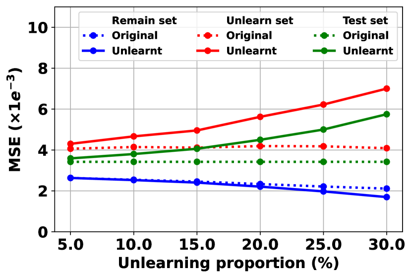
(a) MSE

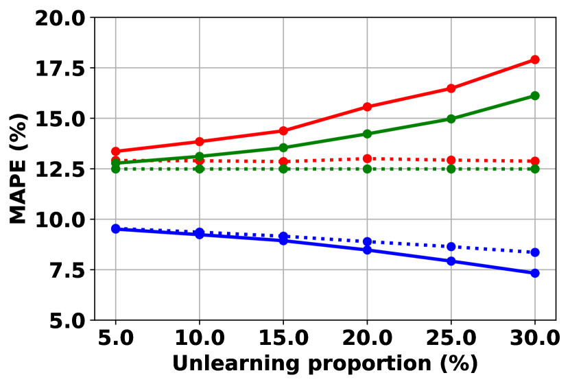
(b) MAPE

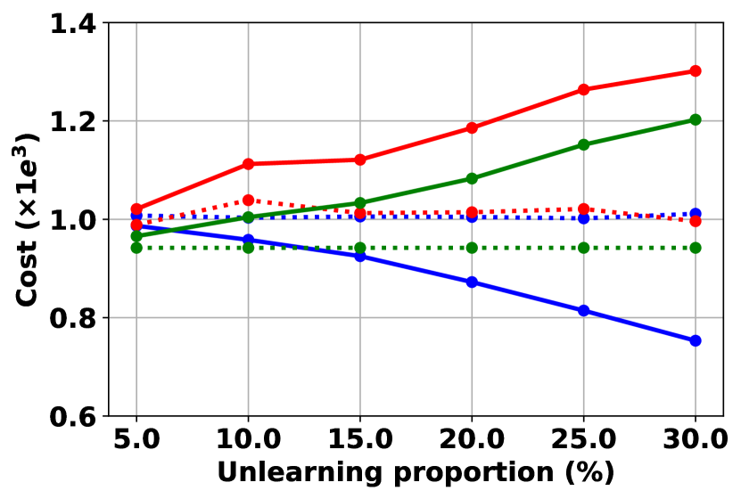
(c) Cost

Figure 4: Unlearning performance on the linear load forecaster using (8). Remain set, Unlearn set, and Test set represent the performance on the corresponding dataset. Original and Unlearnt represent the performance of the dataset evaluated by the original and unlearnt models.

The unlearning performances on the linear load forecasting model are summarized in Fig.4. We have verified that the unlearning algorithm (8) results in the same updated parameter as the one re-trained on the remaining dataset under all unlearning rates, verifying the golden rule of unlearning.

Note that the dotted curves, which represent the performance of the original model, only slightly change across the various unlearning ratios. Broadly speaking, the performance gaps between the unlearnt and original models becomes larger as the unlearning ratio increases. Meanwhile, the performances on the remaining dataset improves as the unlearning ratio increases. This is because when the original model is unlearnt, the model parameters are updated and fitted more on the remaining dataset. In contrast, the performances on the unlearnt and test datasets become worse, which verifies the statement that unlearning can inevitably degrade the generalization ability of the trained model. Moreover, it can be observed that the trends of performance changes of the unlearnt model are distinct for different criteria. In detail, the generator cost (Fig.4(c)) diverges more significantly from the original model, compared to the MSE and MAPE.

V-B2 Performance Sensitivity Analysis

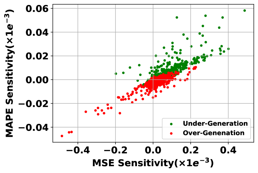
(a) MSE and MAPE ($\bm{r=0.829}$)

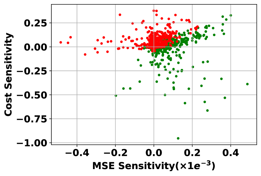
(b) MSE and Cost ($\bm{r=0.073}$)

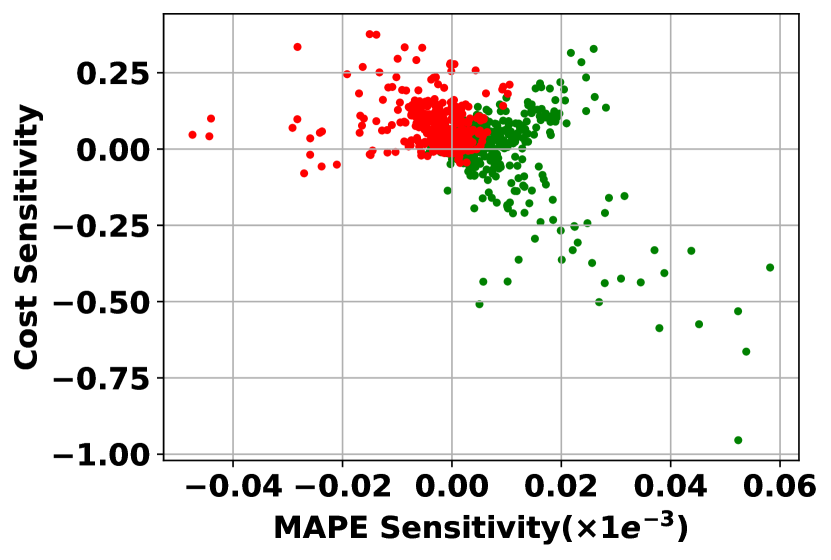
(c) MAPE and Cost ($\bm{r=-0.480}$)

Figure 5: Relationship on the sensitivities of MSE, MAPE, and Cost criteria on the test dataset to the samples in remaining dataset. The $r$ values are Pearson correlation coefficients.

To better show the distinct impact of unlearning on the statistic and task-aware criteria, we draw the sensitivity of the distinct criterion on the test dataset to the samples in the remaining dataset. The remaining dataset is chosen as it is re-weighted in PAMU and TAMU. We randomly sample 1k samples with equal size of under- and over-generation cases. Here, the under-generation implies that the forecast load is lower than the ground-truth load and the over-generation is opposite. We then calculate the sensitivity of each of 1k samples on three criteria on the test dataset by (13) and (15). The relationships of any two of the criteria are illustrated in Fig.5 with associated Pearson correlation coefficients (the $r$ value) highlighted. Since the performance changes are modelled linearly by first-order Taylor expansion (10) and the objective of re-weighting optimization is also linear (16), Pearson correlation coefficient is a suitable indicator of the linear relationship. In Fig.5, positive sensitivity represents the performance degradation after unlearning such sample. I.e., after this sample is unlearnt, the MSE, MAPE, or average generator cost on test dataset increases.

First, the Pearson correlation coefficients have clearly demonstrated that there exists strong positive linear relationship between the two statistic criteria (0.829) while this relationship is insignificant between statistic and task-aware criteria (0.073 between MSE and Cost and -0.480 between MAPE and Cost). These distinct relationships imply that balancing the performance by one statistic criterion is likely effective on the other. In contrast, balancing the performance by statistic criteria can unlikely be effective on the generator cost and vice versa. Secondly, as the under-generation is more costly than the over-generation, unlearning an under-generation sample tends to reduce the overall generator cost with negative sensitivities. As shown by Fig.5(b) and Fig.5(c), if the sensitivities are projected to the y-axis, most of the negative sensitivities are contributed by the under-generation samples, which verifies our intuition. However, it does not occur in MSE and MAPE as they are almost centrally symmetric around the origin in Fig.5(a).

The above discussions can verify the intuition that the statistic performance cannot reflect and may even conflict on the task-aware operation cost.

V-B3 Performances of PAMU and TAMU

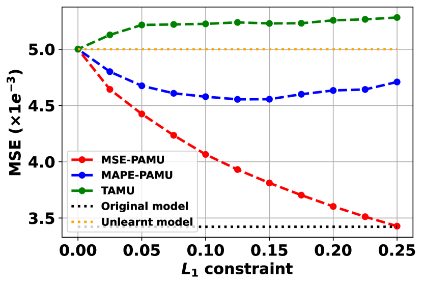
(a) MSE

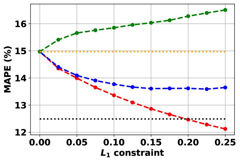
(b) MAPE

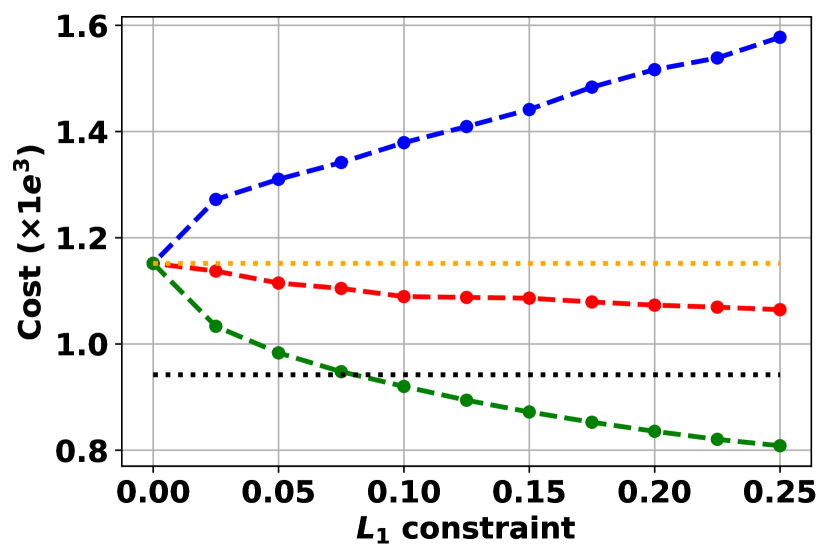
(c) Cost

Figure 6: Performance of PAMU and TAMU with different test criteria. a), b), and c) are performances on the test dataset evaluated by MSE, MAPE, and average generator cost, respectively.

The performances of PAMU and TAMU on the test dataset are reported in Fig.6 in which 25% training data is removed. To balance the MU completeness and performance degradation, $\lambda_{1}$ is varied. The inf-norm constraint $\lambda_{\infty}$ in (16) is set as 1. I.e., the weight of a remaining sample can very from 0 to 2. First, as shown by Fig.6, unlearning by balancing one of the criteria can significantly keep the performance of the the same criterion (e.g., red curve in Fig.6(a), blue curve in Fig.6(b), and green curve in Fig.6(c)). When $\lambda_{1}$ approaches to 0, the PAMU and TAMU become complete unlearning algorithm with the same performance as the retrained model in all criteria, as no samples can be re-weighted. When $\lambda_{1}$ increases, the performance on the original model is recovered and the divergence to the retrained model increases. After $\lambda_{1}$ is further increased, a better performance is attained, resulting in a new type of continual learning through sample re-weighting. As a result, the proposed PAMU and TAMU can effectively balance the completeness and performance trade-off in MU by changing $\lambda_{1}$. In addition, Fig.7 illustrates the parameter difference to the retrained model (evaluated by 2-norm) vs the generator cost, which clearly demonstrates the trade-off as well.

Meanwhile, it is observed that the cost curves perform differently compared to the MSE and MAPE curves. When balancing the cost, both MSE and MAPE get worse. In contrast, balancing the MSE can also keep/improve the MAPE performance, and visa versa. This observation is in line with the analysis on the Pearson correlation coefficient in the previous section.

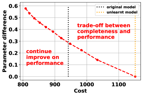
Figure 7: Trade-off between MU completeness and the operation cost.

V-C Unlearning Performance on the NN Forecaster

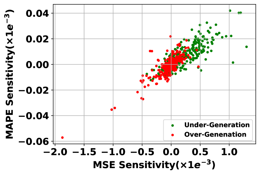
(a) MSE and MAPE ($\bm{r=0.831}$)

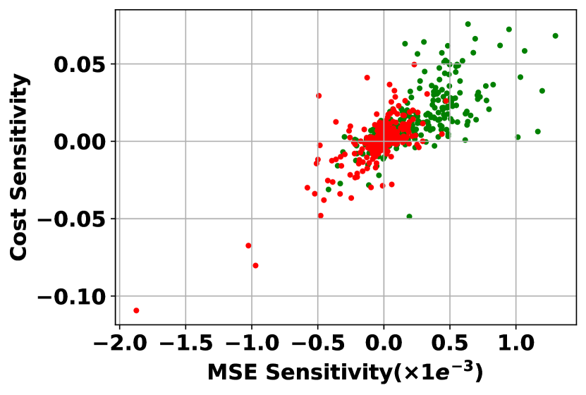
(b) MSE and Cost ($\bm{r=0.730}$)

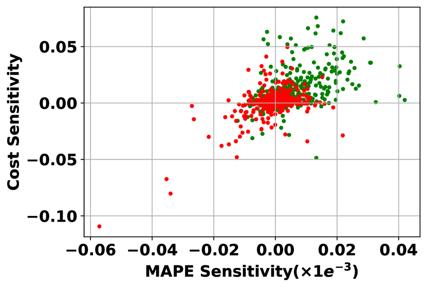
(c) MAPE and Cost ($\bm{r=0.520}$)

Figure 9: Relationship on the sensitivities of MSE, MAPE, and Cost metrics of NN based load forecaster.

Since the fine fine-tuning objective on $\mathcal{D}_{\text{sen}}$ is quadratic (Proposition 2), the direct unlearning is also complete for NN load forecaster. We can expect the unlearning behaviours are similar to the linear counterpart. Therefore, we only highlight some of the simulation results and leave details in Appendix -E. The sensitivities shown by Fig.9 have different patterns to the linear counterpart in Fig.5. Although the linear relationship is more significant between statistic and task-aware criteria, it is still less significant than it within the statistic criteria. This results in balancing any one of the considered criteria can also maintain the remaining two to some extent, as shown by Fig.10.

VI Conclusion

This paper introduces machine unlearning algorithm for load forecasting model to eliminate the influence of data that is adversarial or contains sensitive information of individuals. Influence function provides theoretical foundations, which is further used to evaluate the impact of unlearning on the performance of test dataset. A performance aware machine unlearning is proposed by re-weighting the remaining dataset. To handle the divergence between the statistic and task-aware criteria, we propose task-aware machine unlearning. The simulation results verify that the proposed task-aware algorithm can significantly reduce the generator cost on the test dataset, by compensating on the unlearning completeness.

-A Power System Operation Models

In the U.S., the following network constrained economic dispatch (NCED) problem is broadly adopted [28]. Given the forecast load $\hat{\bm{y}}$ on each bus,

$$(\bm{P}_{g}^{\star},\bm{\vartheta}^{\star},\bm{s}^{\star})= \arg\min_{\bm{P}_{g},\bm{\vartheta},\bm{s}}\bm{P}_{g}^{T}\bm{Q}_{g}\bm{P}_{g}+\bm{c}_{g}^{T}\bm{P}_{g}+c_{ls}\|\bm{s}\|_{1}$$

s.t. $$\underline{\bm{P}}_{g}\leq\bm{P}_{g}\leq\bar{\bm{P}}_{g}$$

$$\bm{B}_{\text{bus}}\bm{\vartheta}=\bm{C}_{g}\bm{P}_{g}-\bm{C}_{l}(\hat{\bm{y}}-\bm{s})$$

$$\underline{\bm{P}}_{f}\leq\bm{B}_{f}\bm{\vartheta}\leq\bar{\bm{P}}_{f}$$

$$\bm{s}\geq 0,\quad\bm{\vartheta}_{\text{ref}}=0$$

A quadratic generator cost is assumed in the dispatch problem. In addition, $\bm{B}_{\text{bus}}$ and $\bm{B}_{f}$ are the bus susceptance and branch succeptance matrices, respectively. $\bm{C}_{g}$ and $\bm{C}_{l}$ are the generator and load incidence matrices, respectively.

After the generators are scheduled, any over- and/or under- generations are penalized when the actual load $\bm{y}$ is realized. In detail, given $\bm{P}_{g}^{\star}$, we consider the following optimization problem modified from [20, 29]:

$$(\bm{P}_{ls}^{\star},\bm{P}_{gs}^{\star},\bm{\vartheta}^{\star})= \arg\min_{\bm{P}_{ls},\bm{P}_{gs},\bm{\vartheta}}c_{ls2}\|\bm{P}_{ls}\|_{2}^{2}+c_{gs2}\|\bm{P}_{gs}\|_{2}^{2}$$

$$\quad\quad+c_{ls1}\|\bm{P}_{ls}\|_{1}+c_{gs1}\|\bm{P}_{gs}\|_{1}$$

s.t. $$\bm{B}_{\text{bus}}\bm{\vartheta}=\bm{C}_{g}(\bm{P}_{g}^{\star}-\bm{P}_{gs})-\bm{C}_{l}({\bm{y}}-\bm{P}_{ls})$$

$$\underline{\bm{P}}_{f}\leq\bm{B}_{f}\bm{\vartheta}\leq\bar{\bm{P}}_{f}$$

$$\bm{P}_{ls}\geq 0,\quad\bm{P}_{gs}\geq 0,\quad\bm{\vartheta}_{\text{ref}}=0$$

where $\bm{P}_{ls}$ and $\bm{P}_{gs}$ are the load shedding and generation storage. The second order cost $c_{gs2}<c_{ls2}$ and linear cost $c_{gs1}<c_{ls1}$ are set to penalize more on the load shedding.

-B Proof to Proposition 1

Consider the following QP:

$$\bm{x}^{\star}= \arg\min_{\bm{x}}\frac{1}{2}\bm{x}^{T}\bm{Q}\bm{x}+\bm{q}^{T}\bm{x}$$ (.1)

s.t. $$\bm{A}\bm{x}+\bm{b}+\bm{g}(\bm{z})\leq\bm{0}$$

$$\bm{C}\bm{x}+\bm{d}+\bm{h}(\bm{z})=\bm{0}$$

where $\bm{x}\in\mathbb{R}^{n}$, $\bm{Q}\in\mathbb{R}^{n\times n}$, $\bm{q}\in\mathbb{R}^{n}$, $\bm{A}\in\mathbb{R}^{m\times n}$, $\bm{b}\in\mathbb{R}^{m}$, $\bm{C}\in\mathbb{R}^{p\times n}$, $\bm{d}\in\mathbb{R}^{p}$, and $\bm{z}\in\mathbb{R}^{q}$. $\bm{g}:\mathbb{R}^{q}\rightarrow\mathbb{R}^{m}$ and $\bm{h}:\mathbb{R}^{q}\rightarrow\mathbb{R}^{p}$ are functions on $\bm{z}$, representing the perturbation parameters. Apart from the linear parametric inequality constraints, we also include the linear parametric term $\bm{g}(\bm{z})$ in the inequality constraint for generalization purpose (and it also gives the same conclusion). We call (.1) as affine-parametric as the parametric terms $\bm{g}(\bm{z})$ and $\bm{h}(\bm{z})$ are affine in the inequality and inequality constraints.

Proposition 3.

Given affine parametric QP (.1), the optimal primal and dual pair $(\bm{x}^{\star},\bm{\lambda}^{\star},\bm{\nu}^{\star})$ is an affine function of the parameter $(\bm{g}(\bm{z}),\bm{h}(\bm{z}))$ if 1). $\bm{Q}$ is positive definite; and 2). the linear independent constraint qualification (LICQ) is satisfied at $(\bm{x}^{\star},\bm{\lambda}^{\star},\bm{\nu}^{\star})$.

Proof.

First, the LICQ states that the gradient of the active constraints (including all equality constraints and active inequality constraints) are linearly independent [30]. Second, the equality Karush–Kuhn–Tucker (KKT) conditions [30] can be denoted as:

$$\bm{G}(\bm{x}^{\star},\bm{\lambda}^{\star},\bm{\nu}^{\star},\bm{z})=\left(\begin{array}[]{c}\bm{Q}\bm{x}^{\star}+\bm{q}+\bm{A}^{T}\bm{\lambda}^{\star}+\bm{C}^{T}\bm{\nu}^{\star}\\ \operatorname{diag}(\bm{\lambda}^{\star})(\bm{A}\bm{x}^{\star}+\bm{b}+\bm{g}(\bm{z}))\\ \bm{C}\bm{x}^{\star}+\bm{d}+\bm{h}(\bm{z})\end{array}\right)=\bm{0}$$

To start, note that $\bm{C}$ is full row rank due to LICQ condition.

When there is no active inequality constraints, $\bm{\lambda}^{\star}=\bm{0}$ due to the complementary slackness. Since $\bm{Q}$ is positive definite, the stationary condition gives that $\bm{x}^{\star}=-\bm{Q}^{-1}(\bm{q}+\bm{C}^{T}\bm{\nu}^{\star})$. From the equality constraint, it can be derived that $\bm{\nu}^{\star}=(\bm{C}\bm{Q}^{-1}\bm{C}^{T})^{-1}(-\bm{C}\bm{Q}^{-1}\bm{q}+\bm{d}+\bm{h}(\bm{z}))$. Note that $\bm{C}\bm{Q}^{-1}\bm{C}^{T}$ is positive definite (thus invertible). Let $\hat{\bm{C}}=\bm{Q}^{-1}\bm{C}^{T}(\bm{C}\bm{Q}^{-1}\bm{C}^{T})^{-1}$, the analytical form for $\bm{x}^{\star}$ can be written as

$$\bm{x}^{\star}=(-\bm{Q}^{-1}+\hat{\bm{C}}\bm{C}\bm{Q}^{-1})\bm{q}-\hat{\bm{C}}(\bm{d}+\bm{h}(\bm{z}))$$ (.2)

which is affined in $\bm{h}(\bm{z})$.

Next, assume there exists some active inequality constraints. Let $\tilde{{\bm{\lambda}}}$, $\tilde{\bm{A}}$, $\tilde{\bm{b}}$, and $\tilde{\bm{g}}(\bm{z})$ are the sub-matrices whose rows are indexed by the active constraints. Therefore, $\bm{A}^{T}\bm{\lambda}^{\star}=\tilde{\bm{A}}^{T}\tilde{\bm{\lambda}}^{\star}$ and the active inequality constraint becomes:

$$\tilde{\bm{A}}\bm{x}^{\star}+\tilde{\bm{b}}+\tilde{\bm{g}}(\bm{z})=0$$ (.3)

Since $\bm{Q}$ is positive definite, the stationary condition gives that

$$\bm{x}^{\star}=-\bm{Q}^{-1}(\bm{q}+\tilde{\bm{A}}^{T}\tilde{\bm{\lambda}}^{\star}+\bm{C}^{T}\bm{\nu}^{\star})$$ (.4)

Plugging (.4) into (.3) and the equality condition gives the following matrix form:

$$\bm{\mathcal{Q}}\left(\begin{array}[]{c}\tilde{\bm{\lambda}}^{\star}\\ \bm{\nu}^{\star}\end{array}\right)=\underbrace{\left(\begin{array}[]{c}-\tilde{\bm{A}}\bm{Q}^{-1}\bm{q}+\tilde{\bm{b}}+\tilde{\bm{g}}(\bm{z})\\ -\bm{C}\bm{Q}^{-1}\bm{q}+\bm{d}+\bm{h}(\bm{z})\end{array}\right)}_{\bm{r}(\bm{z})}$$ (.5)

where

$$\bm{\mathcal{Q}} =\left(\begin{array}[]{cc}\tilde{\bm{A}}\bm{Q}^{-1}\tilde{\bm{A}}^{T}&\tilde{\bm{A}}\bm{Q}^{-1}\bm{C}^{T}\\ \bm{C}\bm{Q}^{-1}\tilde{\bm{A}}^{T}&\bm{C}\bm{Q}^{-1}\tilde{\bm{C}}^{T}\end{array}\right)$$

$$=\left(\begin{array}[]{c}\tilde{\bm{A}}\\ \bm{C}\end{array}\right)\bm{Q}^{-1}\left(\begin{array}[]{cc}\tilde{\bm{A}}^{T}&\bm{C}^{T}\end{array}\right)$$

Due to LICQ, $(\tilde{\bm{A}}^{T},\bm{C}^{T})$ is full column rank. Therefore, $\bm{\mathcal{Q}}$ is positive definite and from (.5)

$$\left(\begin{array}[]{c}\tilde{\bm{\lambda}}^{\star}\\ \bm{\nu}^{\star}\end{array}\right)=\bm{\mathcal{Q}}^{-1}\bm{r}(\bm{z})$$ (.6)

which is affine in $(\tilde{\bm{g}}(\bm{z})^{T},\bm{h}(\bm{z})^{T})^{T}$.

Consequently, plugging (.6) into (.4) gives

$$\bm{x}^{\star}=-\bm{Q}^{-1}\left(\bm{q}+(\tilde{\bm{A}}^{T},\bm{C}^{T})\bm{\mathcal{Q}}^{-1}\bm{r}(\bm{z})\right)$$ (.7)

which is affine in $(\tilde{\bm{g}}(\bm{z})^{T},\bm{h}(\bm{z})^{T})^{T}$.

∎

Since the optimal solution of every QP satisfying Proposition 3 is an affine function of parameter ((.2) and (.7)), the gradients of the convex layers exist and can be analytically written regardless of the perturbed parameter.

-C Proof to Proposition 2

Let $\bm{f}(\cdot;\bm{\theta}_{\text{FE}}^{\star})$ be the trained feature extractor on the core dataset. Let $\bm{X}_{\text{sen}}\in\mathbb{R}^{N_{\text{sen}}\times d}$ be the extracted feature of $\mathcal{D}_{\text{sen}}$ as input to the Linear Layer 2. $N_{\text{sen}}$ is the number of user sensitive data and $d$ is the output size of feature extractor. Note that $d\ll N_{\text{sen}}$ and $\bm{X}_{\text{sen}}$ is full column rank. Meanwhile, let $\bm{Y}_{\text{sen}}\in\mathbb{R}^{N_{\text{sen}}\times n}$ be the ground truth load over $n$ participants. The parameter of Linear Layer 2 is denoted as $\bm{\Theta}\in\mathbb{R}^{d\times n}$.

Let $\bm{y}_{\cdot,i}\in\mathbb{R}^{N_{\text{sen}}}$ and $\bm{\theta}_{\cdot,i}\in\mathbb{R}^{d}$ be the $i$-th column of $\bm{Y}_{\text{sen}}$ and $\bm{\Theta}$, respectively. The fine tuning objective can be written as

$$\mathcal{L}(\bm{\theta})=\frac{1}{N_{\text{sen}}\cdot n}\sum_{i=1}^{n}\|\bm{y}_{\cdot,i}-\bm{X}_{\text{sen}}\bm{\theta}_{i}\|_{2}^{2}$$ (.8)

Now define $\hat{\bm{X}}_{\text{sen}}=\text{diag}([\underbrace{\bm{X}_{\text{sen}},\cdots,\bm{X}_{\text{sen}}}_{n}])\in\mathbb{R}^{N_{\text{sen}}n\times dn}$ as a block diagonal matrix packed by $n$ $\bm{X}_{\text{sen}}$s. $\hat{\bm{Y}}_{\text{sen}}=[\bm{y}_{\cdot,1}^{T},\cdots,\bm{y}_{\cdot,n}^{T}]^{T}\in\mathbb{R}^{N_{\text{sen}}n}$ and $\hat{\bm{\Theta}}=[\bm{\theta}_{\cdot,1}^{T},\cdots,\bm{\theta}_{\cdot,n}^{T}]^{T}\in\mathbb{R}^{dn}$ be the flattened version of $\bm{Y}_{\text{sen}}$ and $\bm{\Theta}$, respectively. It can be verified that (.8) is equivalent to

$$\mathcal{L}(\bm{\theta})=\frac{1}{N_{\text{sen}}\cdot n}\left(\hat{\bm{\Theta}}^{T}\hat{\bm{X}}_{\text{sen}}^{T}\hat{\bm{X}}_{\text{sen}}\hat{\bm{\Theta}}-2\bm{Y}_{\text{sen}}^{T}\hat{\bm{X}}_{\text{sen}}\hat{\bm{\Theta}}+\hat{\bm{Y}}_{\text{sen}}^{T}\hat{\bm{Y}}_{\text{sen}}\right)$$ (.9)

Since $\bm{X}_{\text{sen}}$ is full column rank, $\hat{\bm{X}}_{\text{sen}}^{T}\hat{\bm{X}}_{\text{sen}}$ is positive definite. Therefore, (.9) and (.8) are quadratic with unique global minimizer.

-D Detailed Experiment Settings

-D1 Data Description

The meteorological features in the Texas Backbone Power System [27] include Temperature (k), Longwave Radiation (w/m2), Shortwave Radiation (w/m2), Zonal Wind Speed (m/s), Meridional Wind Speed (m/s), and Wind Speed (m/s) which are normalized based on their individual mean and standard deviation. The calendar feature includes the cosine and sin of the Weekday in a week and Hour in a day according to their individual period. Therefore, a single datum is $(\bm{x}^{i},\bm{y}^{i})\in\mathbb{R}^{14\times 10}\times\mathbb{R}^{14}$. We also normalize the target load by their mean and std. Meanwhile, we use the first 80% data as training dataset and the remaining as test dataset. At last, the IEEE bus-14 system is modified from PyPower.

-D2 Linear Load Forecaster

The linear load forecaster can be found by

$$\min_{\bm{\theta}}\frac{1}{N\cdot 14}\sum_{i=1}^{N}\|\bm{x}^{i}\bm{\theta}-\bm{y}^{i}\|_{2}^{2}$$

where $\bm{\theta}\in\mathbb{R}^{10}$. The quadratic objective can be solved analytically or by using conjugate gradient descent.

-D3 NN Load Forecaster

A convolutional neural network is used as feature extractor, which is summarised in Table.II.

Table II: Structure of the NN load forecasting model. For the convolutional layer, $(k:w\times h+s+p)$ represents the $k$ number of filters, kernel size $w\times h$ with $s$ stride and $p$ padding in both sides. For the linear layer, the number indicates the output size. The activation function is written in bracket.

Conv Layer 1	8: 3 $\times$ 3 + 1 + 1 (relu)
Conv Layer 2	8: 4 $\times$ 4 + 2 + 1 (relu)
Linear Layer 1	64 (tanh)
Linear Layer 2	14

We select the first 30% in the training dataset as the core dataset and the remaining as the user-sensitive dataset. The NN forecaster is trained with 100 epochs, batch size of 16, Adam optimizer with learning rate of $10^{-4}$ and cosine annealing. We also use early stop and record the model with the best performance.

-E Extra Experiment Results

The detailed unlearning performance on the neural network based load forecasting model can be found in Fig.8 to Fig.10.

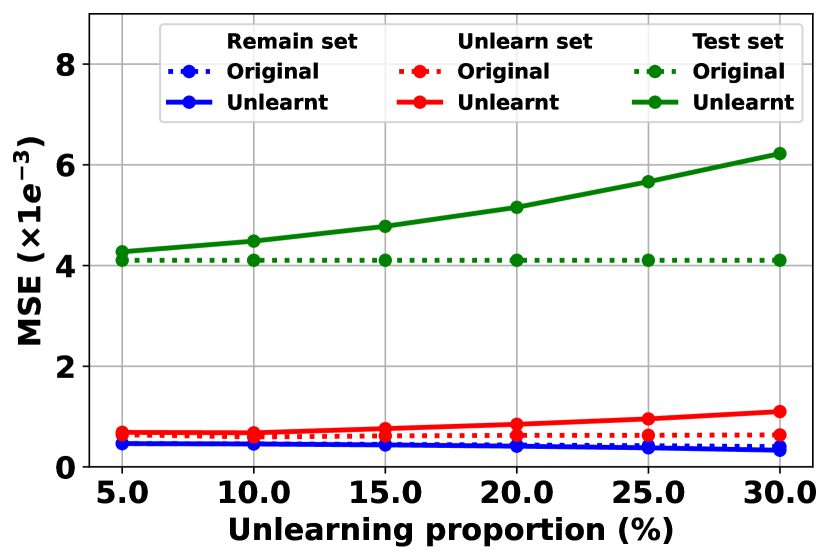
(a) MSE

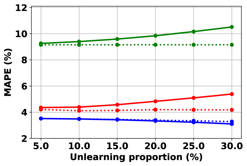
(b) MAPE

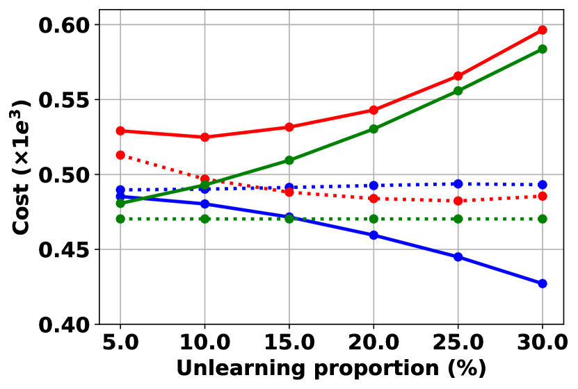
(c) COST

Figure 8: Unlearning performance on the NN based load forecaster.

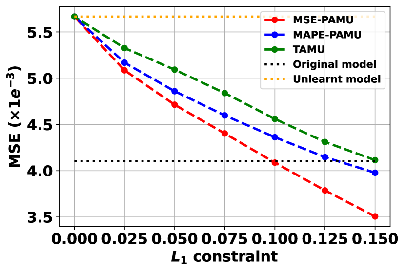
(a) MSE

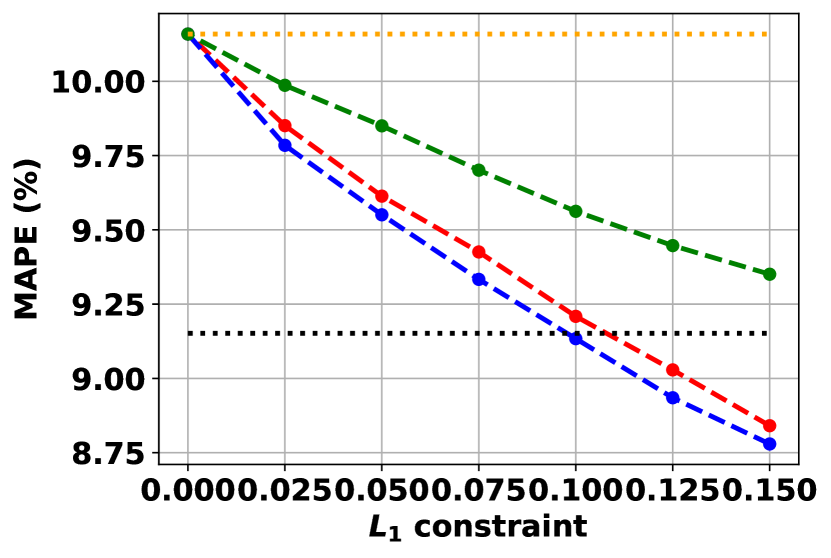
(b) MAPE

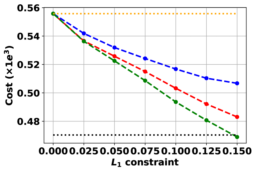
(c) Cost

Figure 10: Performance of PAMU and TAMA with different test criteria for NN based load forecaster.

References

- [1] J. Xie, T. Hong, and J. Stroud, “Long-term retail energy forecasting with consideration of residential customer attrition,” IEEE Transactions on Smart Grid, vol. 6, no. 5, pp. 2245–2252, 2015.
- [2] T. Hong and S. Fan, “Probabilistic electric load forecasting: A tutorial review,” International Journal of Forecasting, vol. 32, no. 3, pp. 914–938, 2016.
- [3] T. Hong, P. Pinson, Y. Wang, R. Weron, D. Yang, and H. Zareipour, “Energy forecasting: A review and outlook,” IEEE Open Access Journal of Power and Energy, vol. 7, pp. 376–388, 2020.
- [4] E. Ebeid, R. Heick, and R. H. Jacobsen, “Deducing energy consumer behavior from smart meter data,” Future Internet, vol. 9, no. 3, p. 29, 2017.
- [5] J. Luo, T. Hong, and S.-C. Fang, “Benchmarking robustness of load forecasting models under data integrity attacks,” International Journal of Forecasting, vol. 34, no. 1, pp. 89–104, 2018.
- [6] Y. Liang, D. He, and D. Chen, “Poisoning attack on load forecasting,” in 2019 IEEE innovative smart grid technologies-Asia (ISGT Asia). IEEE, 2019, pp. 1230–1235.
- [7] Y. Wang, N. Gao, and G. Hug, “Personalized federated learning for individual consumer load forecasting,” CSEE Journal of Power and Energy Systems, 2022.
- [8] Y. Dong, Y. Chen, X. Zhao, and X. Huang, “Short-term load forecasting with distributed long short-term memory,” arXiv preprint arXiv:2208.01147, 2022.
- [9] E. U. Soykan, Z. Bilgin, M. A. Ersoy, and E. Tomur, “Differentially private deep learning for load forecasting on smart grid,” in 2019 IEEE Globecom Workshops (GC Wkshps). IEEE, 2019, pp. 1–6.
- [10] J. D. Fernández, S. P. Menci, C. M. Lee, A. Rieger, and G. Fridgen, “Privacy-preserving federated learning for residential short-term load forecasting,” Applied Energy, vol. 326, p. 119915, 2022.
- [11] M. A. Husnoo, A. Anwar, N. Hosseinzadeh, S. N. Islam, A. N. Mahmood, and R. Doss, “A secure federated learning framework for residential short term load forecasting,” IEEE Transactions on Smart Grid, 2023.
- [12] A. Mantelero, “The eu proposal for a general data protection regulation and the roots of the ‘right to be forgotten’,” Computer Law & Security Review, vol. 29, no. 3, pp. 229–235, 2013.
- [13] T. T. Nguyen, T. T. Huynh, P. L. Nguyen, A. W.-C. Liew, H. Yin, and Q. V. H. Nguyen, “A survey of machine unlearning,” arXiv preprint arXiv:2209.02299, 2022.
- [14] A. Golatkar, A. Achille, and S. Soatto, “Eternal sunshine of the spotless net: Selective forgetting in deep networks,” in Proceedings of the IEEE/CVF Conference on Computer Vision and Pattern Recognition, 2020, pp. 9304–9312.
- [15] A. Golatkar, A. Achille, A. Ravichandran, M. Polito, and S. Soatto, “Mixed-privacy forgetting in deep networks,” in Proceedings of the IEEE/CVF Conference on Computer Vision and Pattern Recognition, 2021, pp. 792–801.
- [16] C. Guo, T. Goldstein, A. Hannun, and L. Van Der Maaten, “Certified data removal from machine learning models,” arXiv preprint arXiv:1911.03030, 2019.
- [17] J. Bae, N. Ng, A. Lo, M. Ghassemi, and R. B. Grosse, “If influence functions are the answer, then what is the question?” Advances in Neural Information Processing Systems, vol. 35, pp. 17 953–17 967, 2022.
- [18] G. Wu, M. Hashemi, and C. Srinivasa, “Puma: Performance unchanged model augmentation for training data removal,” in Proceedings of the AAAI Conference on Artificial Intelligence, vol. 36, no. 8, 2022, pp. 8675–8682.
- [19] R. Vohra, A. Rajaei, and J. L. Cremer, “End-to-end learning with multiple modalities for system-optimised renewables nowcasting,” arXiv preprint arXiv:2304.07151, 2023.
- [20] P. Donti, B. Amos, and J. Z. Kolter, “Task-based end-to-end model learning in stochastic optimization,” Advances in neural information processing systems, vol. 30, 2017.
- [21] R. D. Cook and S. Weisberg, Residuals and influence in regression. New York: Chapman and Hall, 1982.
- [22] P. W. Koh and P. Liang, “Understanding black-box predictions via influence functions,” in International conference on machine learning. PMLR, 2017, pp. 1885–1894.
- [23] A. Agrawal, B. Amos, S. Barratt, S. Boyd, S. Diamond, and J. Z. Kolter, “Differentiable convex optimization layers,” Advances in neural information processing systems, vol. 32, 2019.
- [24] F. Zhuang, Z. Qi, K. Duan, D. Xi, Y. Zhu, H. Zhu, H. Xiong, and Q. He, “A comprehensive survey on transfer learning,” Proceedings of the IEEE, vol. 109, no. 1, pp. 43–76, 2020.
- [25] B. A. Pearlmutter, “Fast exact multiplication by the hessian,” Neural computation, vol. 6, no. 1, pp. 147–160, 1994.
- [26] S. Diamond and S. Boyd, “Cvxpy: A python-embedded modeling language for convex optimization,” The Journal of Machine Learning Research, vol. 17, no. 1, pp. 2909–2913, 2016.
- [27] J. Lu, X. Li, H. Li, T. Chegini, C. Gamarra, Y. Yang, M. Cook, and G. Dillingham, “A synthetic texas backbone power system with climate-dependent spatio-temporal correlated profiles,” arXiv preprint arXiv:2302.13231, 2023.
- [28] A. J. Conejo and L. Baringo, Power system operations. Springer, 2018, vol. 11.
- [29] J. Zhang, Y. Wang, and G. Hug, “Cost-oriented load forecasting,” Electric Power Systems Research, vol. 205, p. 107723, 2022.
- [30] N. Jorge and J. W. Stephen, Numerical optimization. Spinger, 2006.