Constructing Population-Specific Atlases from Whole Body MRI: Application to the UKBB

Abstract

Population atlases are commonly utilised in medical imaging to facilitate the investigation of variability across populations. Such atlases enable the mapping of medical images into a common coordinate system, promoting comparability and enabling the study of inter-subject differences. Constructing such atlases becomes particularly challenging when working with highly heterogeneous datasets, such as whole-body images, where subjects show significant anatomical variations. In this work, we propose a pipeline for generating a standardised whole-body atlas for a highly heterogeneous population by partitioning the population into meaningful subgroups. We create six whole-body atlases that represent a healthy population average using magnetic resonance (MR) images from the UK Biobank dataset. We furthermore unbias them, and this way obtain a realistic representation of the population. In addition to the anatomical atlases, we generate probabilistic atlases that capture the distributions of abdominal fat and five abdominal organs across the population. We demonstrate different applications of these atlases, using the differences between subjects with medical conditions such as diabetes and cardiovascular diseases and healthy subjects from the atlas space. With this work, we make the constructed anatomical and label atlases publically available and anticipate them to support medical research conducted on whole-body MR images. They are available for download at this address.

Introduction

Magnetic resonance imaging (MRI) is a powerful non-invasive imaging technique that can aid the diagnosis and monitoring of diseases along with treatment planning [Brown1999MagneticRI]. These medical images build a valuable basis for medical research, especially if they are available for large cohorts (such as the UK Biobank [ukbb]). They allow for an investigation of inter-subject differences, anomalies, or the comparison of different populations.

Despite all benefits of large medical imaging cohorts, they come with a significant challenge: a lack of comparability between individual subjects, which can, for example, stem from the utilisation of different scanners or different protocols. But even unavoidable natural anatomical differences between subjects complicate the comparison among them. One solution to this problem is the introduction of medical atlases. They define a common reference space for all images and represent an average image derived from the whole cohort. To this end, all images of a cohort are registered into a common reference space, enabling a morphological and functional comparison across subjects (inter-subject), groups of subjects (population analysis), or even between the same subject over time (longitudinal analysis) [maurer1993review].

Medical atlases have shown great potential to improve research and medical assessment. They can, for example, be used to guide image segmentation by propagating segmentations to new images. By using an atlas and a matching segmentation, the latter can be propagated to new images that only need to be registered to the atlas. This highly facilitates the complex task of segmenting new regions of interest [cabezas2011review] and gives means to performing segmentation tasks, even if available resources are limited. Furthermore, atlases can be used to detect anomalies. By comparing an individual image to the average representation of a population (the atlas), discrepancies can be identified that can detect unusual pathologies [Sjholm2019AWF] and can support disease detection [Nowinski2021TowardsAA].

So far, most medical atlases are generated and applied in the field of brain imaging [Nowinski2021TowardsAA]. There has been a significant surge in the number of human brain atlas projects, driven by well-funded initiatives such as The BRAIN Initiative [insel2013nih], The Human Brain Project [SALLES2019380], and The Human Connectome Project [elam2021human], to only name a few. These projects aim to advance neuroscience discovery, decode the human brain, study brain circuits and behaviour, map gene expression, obtain ultra-high resolution neuroimages, simulate neocortical micro-circuitry, and understand the brain and its disorders. As a result, the study and the understanding of the human brain are dynamically changing over time as new acquisition techniques, sophisticated applications, tools, and novel concepts are developed [Nowinski2021TowardsAA].

Despite their success in brain imaging, there has been little focus on constructing atlases for more global representations of the human body, such as whole-body imaging datasets, which enable the global assessment of body composition and provide a homogeneous overview of the entire body. One reason is that the registration of whole-body images between different subjects and longitudinally within the same subject is particularly challenging, given the high variability between images. This stems from greatly heterogeneous body compositions throughout the population. While brain images maintain high comparability, even if subjects vary in age, sex, height, or weight, whole-body images expose these differences more clearly. Furthermore, there is a lack of whole-body image datasets in particular from healthy subjects, due to the time- and cost-intensive scan procedures. This is targeted by large-scale population-wide studies such as the UK Biobank [ukbb] or the German National Cohort (NAKO) [bamberg2015whole].

There are, however, a few works investigating the generation and application of whole-body atlases. Still, they have yet to become as popular in the analysis of these images as their counterpart of the brain. A potential reason for this could be the fact that most of the currently available whole-body atlases come with major limitations that bound their generalisability: they are often limited in the number of utilised samples, or based on very homogeneous datasets, that only represent a small subset of the whole population. This strongly limits their generalisability to a larger population. Hofmann et al. [hofmann2011mri], for example, shows the usage of whole-body atlases for Positron Emission Tomography (PET) attenuation correction, and Karlsson et al. [karlsson2015automatic] for muscle volume quantification. However, both works use only about $10$ subjects for atlas construction. Sjholm et al. [Sjholm2019AWF] propose a multimodal whole-body atlas of functional 18F-fluorodeoxyglucose (FDG) PET and anatomical fat-water MR data and show its utility for anomaly detection. This atlas is constructed from only $27$ subjects ($15$ female, $12$ male). An atlas based on a larger dataset of $128$ MRI scans from the POEM database ($68$ female, $60$ male) was proposed by Strand et al. [strand2017concept]. However, this study focuses on the analysis of $50$-year-old subjects only, limiting the atlas to a very homogeneous subset of the population. The authors study pathophysiological links between obesity, vascular dysfunction, and future cardiovascular disorders, forming a weight loss and gastric bypass study. Using a similar amount of data ($250$ subjects), Joensson et al. [jonsson2022image] propose an image registration method of whole-body PET-CT images to quantify spatial tumour distributions and capture tissue and muscle mass loss from pre- and post-therapy images. Lind et al. [lind2019proof] propose to visualise how fat and lean tissue mass are associated with local tissue volume and fat content by utilising whole-body quantitative water-fat MRI and DXA scans of $159$ men and $167$ women aged $50$ in the population-based POEM study. The dataset restriction to a homogeneous distribution for the construction of whole-body atlases emphasises both the complexity of the task, as well as the need for more work in this area.

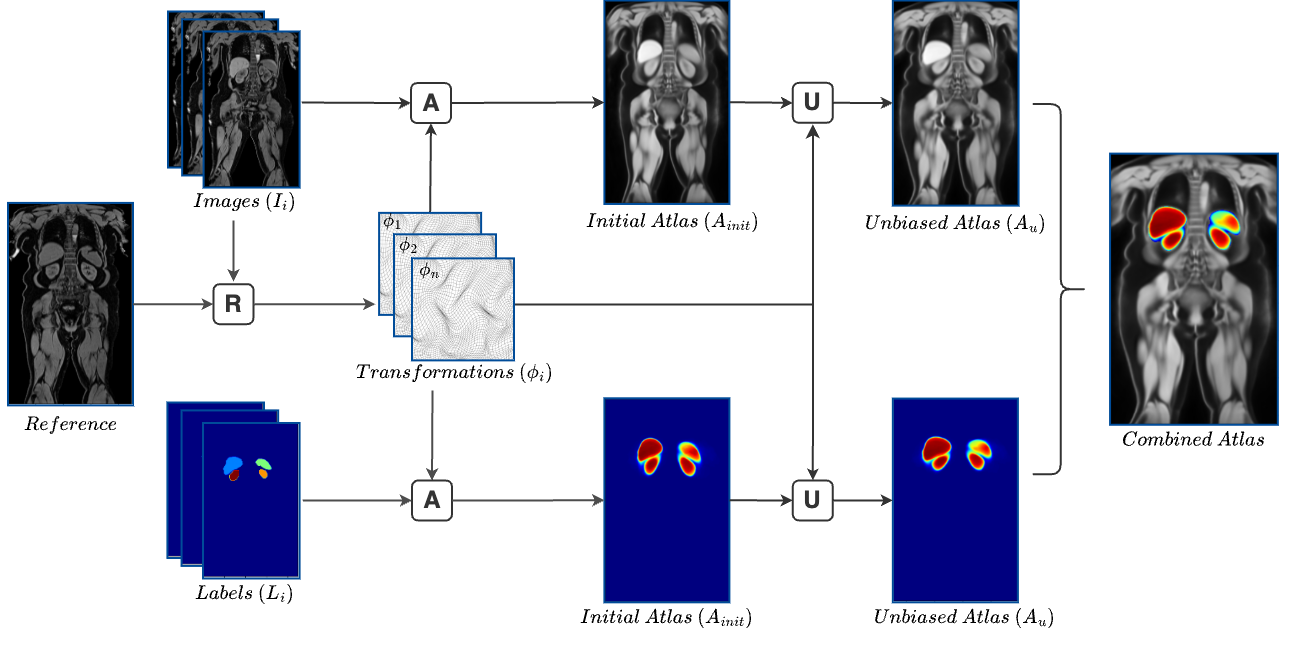
Figure 1: An overview of the processing pipeline for the generation of the whole-body atlases for each group. The first step is to register all images $I_{i}$ to the reference [R], then all images $I_{i}$ and labels $L_{i}$ are warped with the resulting deformation fields $\phi_{i}$ and aggregated in an initial atlas $A_{init}$ [A], the atlases are subsequently unbiased $A_{u}$ [U] in order to create the final anatomical and label atlases.

Given these current limitations and the potential of atlas-based research, we investigate the generation of large-scale whole-body atlases on MR images. Our contributions are as follows:

• We introduce a pipeline that allows for generating whole-body, unbiased atlases, considering the high heterogeneity of whole-body MR images.

• We propose to partition the whole population into six distinct physiological groups based on sex and body mass index (BMI).

• For each group, we generate an unbiased anatomical atlas and label atlases for abdominal subcutaneous and visceral fatty tissue and five abdominal organs.

• We demonstrate applications for these atlases for detecting population subgroup differences between healthy and diseased subjects.

We note that the categorisation utilised in this work functions as a medically motivated example, whereas our pipeline can be used for arbitrary subgroupings. We hope to facilitate further research in this area by making these large-scale whole-body atlases publicly available.

Methods

In this section, we give an overview of the utilised dataset and summarise the applied methods, including the selection criteria for the images, the registration pipeline, and the generation of the atlases, followed by a final unbiasing step. An overview of the atlas generation pipeline is visualised in Figure 1.

Dataset

The atlases provided in this work are constructed from the whole-body MR images from the UK Biobank dataset, a large-scale biomedical database and research resource, containing […] genetic and health information from half a million UK participants [ukbb]. It is an ongoing longitudinal study performed in the UK and represents a selection across the population in the UK with an age range of the subjects between $40$ and $80$. Additionally to a large selection of phenotypic and lifestyle information, it contains several imaging data types such as brain, heart or whole-body MR at different time points. The UK Biobank currently provides ca. $50\,000$ T1-weighted, dual-echo gradient whole-body MR images with a size of $224\times 168\times 363$ voxels and a resolution of $2,232\times 3\times 2,23$ mm. They contain 4 Dixon contrasts: water, fat, in-phase and out-of-phase. These scans were acquired in six individual stations and, in a post-processing step, merged using a public stitching tool [lavdas2019machine]. This way, one image from neck to knee is generated for each subject. This study utilises $3\,000$ of the stitched water-contrast images, the selection process is described in the following paragraph and example images are shown in Figure 2. We extract segmentations for abdominal organs and abdominal fat, following the pipelines proposed in [org-seg] and [Kstner2020FullyAA]. The organ segmentations are extracted for the liver, the spleen, the pancreas, the left and the right kidney and the fat segmentations are divided into abdominal subcutaneous and visceral fatty tissue. We note that the fat segmentation algorithm only targets abdominal fat identification, not considering fatty tissue in other parts of the body, such as the legs. Additionally, the data distribution of the UK Biobank, in terms of ethnicity, is highly unbalanced towards white British subjects. We, therefore, note that our atlases contain the same inherent imbalance.

Data Selection

Given the high intra-subject physiological variability, we consider one single atlas insufficient to represent the entire cohort. Thus, we separate the dataset into six groups based on BMI and sex. We generate one anatomical atlas and corresponding label atlases for each of the following subject groups: (1) females with normal BMI, (2) overweight females, (3) obese females, (4) males with normal BMI, (5) overweight males, and (6) obese males. Table 1 indicates the specific BMI ranges for each group.

For the generation of each atlas, a set of approximately $500$ subjects in each category (matching BMI and sex) is selected. To generate a representation of a healthy population, we only select subjects that have no record of cancer, no self-reported diseases, and no operation history. From the set of all subjects that meet those criteria, we sample $500$ individuals randomly, except for the male obese subgroup, where only $471$ subjects meet the selection criteria, and all are used for the atlas generation. We chose $500$ subjects for each atlas due to the limited amount of healthy subjects in each category. This way, all atlases are based on a similar amount of subjects.

Atlas Generation Pipeline

In the following, we introduce our atlas generation pipeline, which is visualised in Figure 1. The first step of generating an atlas requires the registration of all images in order to align the whole dataset in one common coordinate space. This is done by choosing a reference image, also called fixed, and registering all remaining moving images of the dataset to it (top left of Figure 1). By applying the resulting transformations to the images as well as the corresponding segmentations, we generate one initial anatomical atlas and several initial label atlases. Finally, all atlases are unbiased to avoid a strong alignment with the reference image.

Category	BMI range	# females	# males
Normal weight	$[18;25[$	$500$	$500$
Overweight	$[25;30[$	$500$	$500$
Obese	$\geq 30$	$500$	$471$

Table 1: Overview of the different BMI categories used to split the data for the atlas generation and the amount of data used per group.

Reference Selection

For each subgroup of the dataset, one reference image has to be selected. This reference image can significantly impact the registration performance and must be carefully selected to optimally represent the distribution in the cohort. We use the phenotypic data of the subjects to identify the most representative reference for each group. All reference subjects represent the median age, weight, height, BMI, and body fat percentage in the respective subgroup of the dataset (e.g. overweight females). The specific properties of all selected reference subjects are summarised in Table 2. A medical expert then assessed the selected references, evaluating whether the muscle and fat proportions were representative of the respective subgroup. Figure 2 shows the final reference images selected for the atlas generations, overlayed with the corresponding abdominal fat segmentations. We can see apparent differences in anatomy and fat distribution between the groups, highlighting the necessity to separate the dataset.

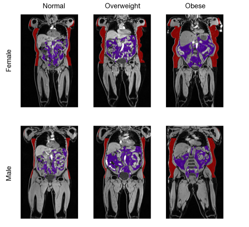
Figure 2: Reference images of the different subgroups of the dataset; The first row shows the female subjects and the second row the male subjects of the respective BMI groups (columns) overlayed with their respective labels of fatty tissue. Red: abdominal subcutaneous fat, purple: abdominal visceral fat.

Sex	BMI Category	Age (years)	Weight (kg)	Height (cm)	BMI	Body fat (%)
Female	Normal weight	63	60.8	164.0	22.6	35.2
	Overweight	64	71.2	163.0	26.8	42.2
	Obese	61	87.6	162.0	33.4	42.0
Male	Normal weight	66	72.9	177.0	23.3	18.5
	Overweight	68	83.1	176.0	26.8	26.3
	Obese	67	101.6	174.0	33.6	31.9

Table 2: Body composition values of the selected reference subjects for each BMI group and sex.

Pre-processing

Although all images are acquired using the same scanner and following the same procedure, imaging data subgroup variability remains high for technical (applied MR sequences) and anatomical (inter-subject variation) reasons, raising challenges for subsequent registration. To mitigate this and subsequently maximise registration performance, we apply two types of normalisation: intensity-based and spatial normalisation. We first perform an intensity-based normalisation in several steps. (1) We ensure the same range of pixel values in all images by min-max normalisation. (2) We enhance the contrast of the images by thresholding the intensity histogram to accentuate boundaries and therefore facilitate registration, and (3) mask out the background of the images using an automatically generated body mask in order to avoid any unwanted impact of the background noise on the registration. Given the substantial anatomical differences between subjects (e.g. height), the dataset shows large variability regarding angles and the fields of view. To address this, we perform a spatial normalisation using a centre of mass initialisation. Within each subgroup, the centre mass of each subject is computed and aligned to the corresponding reference’s centre of mass, with an iterative closest point (ICP) method using the open-source library by [Zhou2018]. This alignment is a global registration initialisation to correct extreme positional differences and aims to facilitate the following registration steps.

Registration

Registration is the key step for constructing an atlas, ensuring a spatial normalisation and mapping all images into the same coordinate space [maurer1993review]. Registration aims to find the best parameters for the selected transformation model that minimise the discrepancy between corresponding features in the two images. This is typically achieved by an optimisation process that minimises a cost function or error metric.

In particular, given a fixed $\mathcal{F}:\Omega_{F}\subseteq\mathbbm{R}^{n}\rightarrow\mathbbm{R}$ and moving image $\mathcal{M}:\Omega_{M}\subseteq\mathbbm{R}\rightarrow\mathbbm{R}^{n}$, image registration aims to find the spatial transformation $\mathcal{\phi}^{*}:\Omega_{F}\rightarrow\Omega_{M}$ which best maps a location $x$ in $\mathcal{M}$ to the location with corresponding tissue or structure in $\mathcal{F}$. This is mathematically described with the following formula:

$$\phi^{*}=\arg\min_{\phi}[\mathcal{D}(\mathcal{F},\mathcal{M}\circ\phi)+\lambda\mathcal{R}_{Reg}],$$ (1)

where $\mathcal{D}$ is a dissimilarity metric between the fixed ($\mathcal{F}$) and the transformed moving image ($\mathcal{M}\circ\mathcal{\phi}$), warped in the coordinate space of the fixed using the transformation $\mathcal{\phi}^{*}$, $\mathcal{R}_{Reg}$ is a regularisation term on the transformation which is furthermore introduced to enforce smoothness and diffeomorphism weighted by a factor $\lambda$.

Whole-body image registration is a non-trivial task due to the strong anatomical differences across subjects and the differences in the angles and field of view. For example, the abdominal region is highly deformable and versatile in position, shape, structure, and size even within a healthy cohort with similar properties (e.g. BMI and sex) due to intractable factors such as breathing motion or volumetric changes. In contrast to the highly deformable regions, there are also rigid structures such as the bones or the spinal cord. These aspects must be considered to perform meaningful whole-body registrations preserving the anatomy.

Affine Registration

As a first step, we register all images using affine registration, i.e., compensate for differences in the translation, rotation, shearing and scaling of the images using the Medical Image Registration ToolKit (MIRTK) [mirtk] software. Following this approach, the general geometric structure of the images is preserved. However, this alignment is insufficient to create a high-quality, detailed atlas. The underlying idea is that affine transformations compensate only for the global misalignment of the images, disregarding their local differences, which is why we also require a deformable registration step.

Deformable Registration

Subsequently, we use the affinely registered images as the starting point to perform deformable registration, also known as non-linear registration. It aims to align the images locally, allowing more complex, spatially varying transformations between points or local features, e.g., organ deformations.

Consequently, we decided to model the transformation $\phi$ as a Stationary Velocity Field (SVF) [Modat2012ParametricNR]-based Free-Form deformation (FFD) [Rueckert2000NonrigidRU] that models the deformation field as velocities on a grid of control points which we have to integrate [Arsigny2006ALF] to get the displacement field. This type of transformation is diffeomorphic and therefore it is topology preserving and invertible, properties that are crucial to our atlas construction process.

Finally, in order to obtain the best possible registration, we perform a grid search over a selected set of hyper-parameters and choose the best-performing ones with respect to three different evaluation metrics which assess the accuracy and the regularity of the registration: (1) The dice score between the reference and the warped anatomical (abdominal organs, whole-body and fat) segmentation labels, (2) the determinant of the Jacobian of the transformation with which we evaluate the number of points in the image resulting in anatomically implausible transformations and (3) the magnitudes of the gradient of the Jacobian determinant that aid us to evaluate the spatial smoothness of the transformation.

The deformable registration is performed using the open-source toolbox Deepali [deepali], which allows for an extremely fast hyperparameter search and registration due to its GPU support.

All parameters used for both affine and deformable registration are reported in the Supplementary Information. The affine registration step can also be performed using Deepali. However, given that we already extracted the affine registration prior to utilising Deepali, we refrain from rerunning this processing step to avoid unnecessarily increasing the environmental impact of this work. We envision similar results when using Deepali for both steps.

(a) Reference image

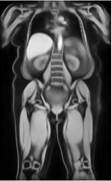
(b) Initial anatomical atlas

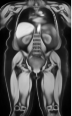
(c) Unbiased anatomical atlas

Figure 3: Atlas unbiasing example for the obese female subgroup. From left to right: the reference image (3(a)), the initial (biased) anatomical atlas (3(b)), and the unbiased atlas (3(c)).

Atlas Generation and Unbiasing

Once the subjects from each group are registered to their corresponding reference image and consequently to the same coordinate space, we construct an initial atlas $A_{\operatorname{init}}$ for each group by averaging the $n$ registered subjects of the group:

$$A_{\operatorname{init}}=\frac{1}{n}\sum_{i=1}^{n}\mathcal{I}_{i}\circ\phi_{i},$$ (2)

where $\mathcal{I}_{i}$ refers to the image of the $i$-th subject in the group and $\phi_{i}$ to its corresponding transformation field. We follow this approach to generate one initial anatomical atlas and all label-based atlases (for abdominal organs and fat) for each subgroup of the dataset.

These initial atlases heavily rely on the choice of reference. Figure 3 shows how similar the reference-specific atlas (3(b)) is to the reference image (3(a)). This atlas still serves as a decent representation of the population, even with this bias, since the reference image was statistically and clinically chosen to represent the subgroup of the population as well as possible. It, however, holds the risk of propagating subject-specific traits to the atlas, which might be mistaken with population traits in further downstream tasks. We introduce an atlas unbiasing [rueckert2003atunb] step to the pipeline to address this. This process utilises the deformation fields and the previously constructed atlas to generate a more realistic representation of the population. We extract an average inverse transformation field $\Phi$ by first inverting the individual transformation fields and then averaging them:

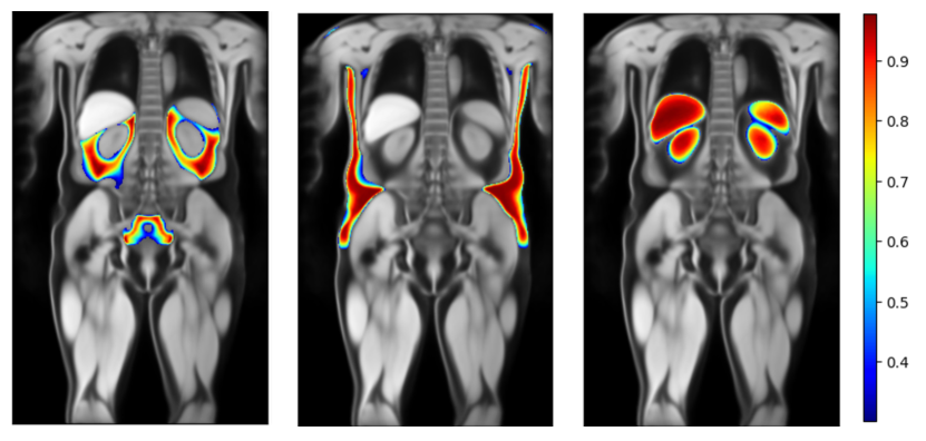
Figure 4: Example atlas of the overweight male subgroup. We visualise one coronal slice of the unbiased anatomical atlas, overlayed with the probability maps of the abdominal visceral fat (left), the abdominal subcutaneous fat (middle), and the abdominal organs (right)

$$\Phi=\frac{1}{n}\sum_{n=1}^{n}\phi_{i}^{-1}.$$ (3)

The unbiased Atlas $A_{\operatorname{u}}$ is then derived by applying the average inverse transformation field $\Phi$ to the initial atlases:

$$A_{\operatorname{u}}=A_{\operatorname{init}}\circ\Phi=A_{\operatorname{init}}\circ\left(\frac{1}{n}\sum_{n=1}^{n}\phi_{i}^{-1}\right).$$ (4)

Results

With this work, we release all six large-scale anatomical atlases for the different population subgroups (based on BMI and sex), as well as the corresponding label atlases of abdominal organs and abdominal fatty tissue. Figure 4 shows an example of these atlases for obese male subjects. As an effort to facilitate research in the area of large-scale body imaging and population studies, we make these atlases publicly available via CERN’s open repository Zenodo, at this address: https://zenodo.org/record/8226039.

Anatomical and Label Atlases

The atlas generation pipeline described above is performed for each different subgroup. This results in several atlases for each group: (1) an anatomical atlas, showing the average anatomy, (2) two fatty tissue atlases for abdominal subcutaneous and visceral fat, and (3) one atlas for each abdominal organ (liver, spleen, pancreas, left and right kidney).

The anatomical atlas allows for a general analysis of the whole body regarding overall shape and structure. In contrast, the label atlases (organs and fat) allow for a more focused study of the distribution of specific structures in the body. Figure 4 shows an example of these atlases, overlaying the visceral (left), the subcutaneous fat (middle) and the organ (right) atlases on the anatomical atlas for the male, overweight subgroup. The label atlases can be interpreted as probability maps, indicating the likelihood of finding a certain structure (e.g., the liver) at a specific position in the atlas. A high value in these probability maps indicates a high concentration or a high probability that this area contains a label over the whole population. A low value, on the other hand, suggests the unlikeliness of a specific region to contain the respective label.

We visualise the results of the atlas unbiasing in Figure 3. It shows the reference image (3(a)), the initial (biased) anatomical atlas (3(b)) and the unbiased anatomical atlas (3(c)) of the female obese BMI subgroup. The unbiased anatomical atlas (3(c)) is still crisp but contains fewer anatomical specificities propagated by the reference. The reference image (3(a)) and the initial atlas (3(b)) are visually very similar, which is especially obvious when looking at the body outline or the liver shape. In contrast, the unbiased atlas (3(c)) is smoother in these areas and not as strongly conditioned on the reference image. We can also see that the unbiased atlas presents more subcutaneous fat than the initial atlas in the hip area, this occurs when most of the population in the subgroup have more fat than the reference in this region. The unbiasing step allows us to capture this deviation from the reference and therefore correct the atlas. This shows how crucial this step is in order to obtain representative atlases for the whole population.

The UKBB provides whole-body MR scans of four different contrasts: water, fat, in-phase, and out-of-phase. So far, all anatomical atlases have been shown using the water-contrast images since we performed the atlas generation on those images. However, the other contrast images can easily be registered to the atlas using the existing corresponding transformations, resulting in atlases for all contrast images, e.g., fat-contrast anatomical atlas.

Clinical Applications

We show the potential clinical value of the generated atlases by showcasing two applications using the anatomical and label atlases. We demonstrate that the atlases can be successfully used to detect changes in distribution for diseased subgroups and to describe a deviation from the atlas in terms of body composition.

Anomaly Detection in Anatomical Atlases

The atlases proposed in this work are systematically built to represent a healthy population. We show their applicability to detect anomalies or physiological deviations from the atlas by performing voxel-based morphometry (VBM) [ashburner2000voxel]. This method is conventionally used to quantify grey or white matter concentration in a voxel-wise fashion. It allows for the identification of regions of interest and holds potential for a more localised study of the brain. VBM is typically done in several steps: first, one or several groups of interest are identified, and then the target tissue is segmented and registered for all subjects across each group. Spatial smoothing is applied to account for extra variability after registration; finally, the groups are compared to each other using voxel-wise statistical testing.

Here, we perform a similar analysis with the fat-contrast anatomical images. We compare subjects with fatty liver disease (steatosis) against the healthy subjects, which were previously used to build the atlas, for the male overweight subgroup. We specifically choose the fat-contrast images rather than another one because fatty tissue is highly contrasted for these images, as we can see in Figure 5(b). We randomly select $200$ subjects with high liver fat and register their fat-contrast images in the same fashion as previously explained to align them to the atlas space. Each image from both groups is then spatially normalised with a Gaussian kernel; this allows each voxel to represent the average of itself and its neighbours, making each voxel comparable between the two groups. We then perform a voxel-wise t-test between the healthy atlas and the pathological group and obtain a voxel-wise p-value map (P-map). We are eligible to perform a t-test given the central limit theorem [central2017Kwak] that states that if we take sufficiently large random samples from the population, their distribution will be approximately normally distributed. Performing simultaneous statistical tests introduces the multiple comparisons problem, which refers to the increased chance of false positives with many tests. We apply a correction for multiple comparisons called False Discovery rate (FDR) to mitigate this effect, and we only retain the significant p-values $p<0.01$ from the corrected P-map. Figure 5(b) shows the significant voxels overlayed on the anatomical atlas for the overweight male subgroup. As expected, these values highlight a significant change, mostly in the liver for subjects with high liver fat. Other areas of adipose tissue are diffusely highlighted, however, this could be due to noise introduced by misregistration.

(a) Fat anatomical atlas

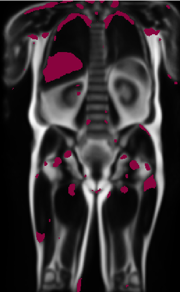
(b) Significant voxels for fatty liver disease

Figure 5: Significant voxels ($p<0.01$) for fatty liver disease subjects for the male overweight subgroup. (5(a)) is the healthy fat-contrast anatomical atlas for the male overweight subgroup and (5(b)) overlays significant voxels for subjects with fatty liver disease compared to healthy subjects.

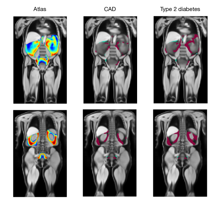
Figure 6: Significant voxels ($p<0.01$) in the visceral fatty tissue for patients with coronary artery disease (middle column) and type 2 diabetes (right column) for the male overweight subgroup. The left column shows the atlas, e.g., the average fat distribution, at two slices. The purple pixels in the second and third column represent more fat in the pathological group and cyan less. This shows that there is significantly more visceral fat in the CAD and diabetic group than in the healthy one.

Distributional Changes in Label Atlases

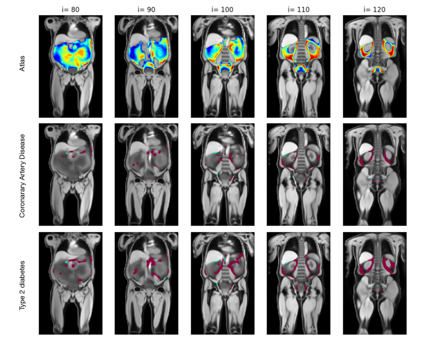
Figure 9: Significant $pval<0.01$ voxels in the visceral fatty tissue for patients with coronary artery disease (middle row) and type 2 diabetes (bottom row) for the male overweight group. The first row shows the atlas, e.g. the average fat distribution, and each column shows a different slice (i) in the image. The purple values represent more fat in the pathological group and the cyan represents less. These results show that there is significantly more visceral fat in the CAD and diabetic group than in the healthy one.

As a second application, we perform a similar analysis with visceral fat distribution. We utilise the abdominal visceral fat maps from healthy subjects previously used to build the atlas of the male overweight group and test them against diseased subjects. The pathological subgroups are selected and registered in the same fashion as previously explained, with the additional criteria that they contain the target disease – in our case, coronary artery disease (CAD) or type 2 diabetes. We select $200$ subjects with CAD, $200$ subjects with diabetes and $200$ subjects from the healthy atlas group. Similarly to before, each fat label map is spatially normalised with a Gaussian kernel, and voxel-wise one-sided t-tests are subsequently performed between the healthy and the pathological group. We perform two types of one-sided t-tests; one assesses a higher mean, which indicates more fat in the pathological group and one the opposite: less fat in the pathological group. The results for both tests are shown in Figure 6, where the significant values for more fat are visualised in purple and those for less fat in cyan. We then perform a FDR correction to the P-map and retain the significant p-values $pval<0.01$. Figure 6 shows the significant voxels overlayed on the anatomical atlas for the overweight male subgroup. The first column shows the fat label atlas overlayed on the water-contrast anatomical atlas; the second column shows the significant voxels for more and less fat for CAD; and the last column for type 2 diabetes. Each row is a visualisation of a different coronal slice. A more comprehensive set of slices can be visualised in the supplementary material in Figure 9.

We see a significant increase in organ-associated visceral fat around the kidneys, as well as in mesenteric fat and within the lower pelvis (Figure 9). Areas of lower fat content are found in the marginal area, as well as on the lower liver border. Moreover, comparing both pathological groups, the diabetic group shows a larger increase in mesenteric fat than the CAD group compared to the atlas. This increase in visceral fat for these pathological groups is also observed in other studies[nakamura1994contribution, despres2007cardiovascular], which further confirms the value of these results. We attribute the marginal speckles (e.g., in the shoulders and lungs) to noise arising from either misregistration or remaining false positives from the t-test.

Discussion and Conclusion

Medical atlases are a powerful tool for spatial normalisation and population-wide analyses of medical images. They have become a staple in neuroimaging research and are now commonly used in most brain analysis pipelines such as VBM [ashburner2000voxel]. However, atlases have been widely under-explored on other medical images, particularly more global representations, such as whole-body scans. The rise of large-scale whole-body datasets such as the UK Biobank [ukbb] or the German National Cohort [bamberg2015whole] opens new possibilities in this area. We make use of the data-rich UK Biobank and generate several large-scale atlases for whole-body MR images and provide a systematic pipeline for atlas generation and population analysis with whole-body images (Figure 1). One challenge of whole-body images is the extremely high inter-subject variability, which is due to the large differences in anatomy, e.g., based on height, sex, age, or BMI. Considering this, we split the dataset of about $3\,000$ subjects into six distinct subgroups by sex and BMI (Table 1) and generate different atlases for each subgroup. We furthermore only select subjects without any self-reported diseases and no record of cancer, in order to obtain a general representation of a healthy population.

For each BMI and sex group, we generate one anatomical atlas, which is based on the water-contrasted whole-body MR images, along with several label atlases, utilising segmentations for five abdominal organs (liver, spleen, pancreas, left and right kidney), as well as visceral and abdominal subcutaneous fatty tissue. These label atlases provide a probabilistic interpretation of the likelihood of a structure of interest (e.g., an organ) to be located at a specific position in the anatomical atlas. They can be used to identify subjects or groups that deviate from the atlas, i.e., anomaly detection, as well as investigating distributional differences between subgroups, for example, assessing how the fat distribution varies. We showcase this by performing t-tests between the atlas and groups of subjects with coronary artery diseases, diabetes and fatty liver disease. With this, we are able to expose variation in distribution between groups at a voxel level. This holds great potential for population studies and group-wise analysis, as it allows for spatial quantification of change. The substantial medical benefit results from the non-invasive, radiation-free measurement of, for example, body composition.

We have shown the application of the label and anatomical atlases in three examples for detecting anomalies and distributional changes in fatty tissue. We see great potential to extend our here-provided atlases with various more label atlases. Muscle tissue, for example, is a strong indicator of age and frailty [evans2010frailty], which would be valuable to integrate into the atlases provided here, along with other label atlases such as the spine, heart, bone, or lung atlases.

A very powerful application of atlases, in general, is label propagation, as it has been extensively demonstrated in the brain [cabezas2011review]. This refers to propagating labels from the atlas to the population, which requires the annotation of only one sample (the atlas), which is very valuable in the medical setting, as it is very cost- and time-effective. As whole-body scans contain many structures worth investigating, we envision label propagation on these anatomical atlases to be very promising.

Another potential application of the atlases would be to leverage them in the context of longitudinal studies. For a subset of the whole dataset, the UK Biobank also provides images acquired at several time points. These could be used to investigate intra-subject developments over time. Furthermore, a comparison between different datasets, such as the NAKO [bamberg2015whole], would show the usability of the atlases beyond one single dataset. By making all generated atlases publicly available, we envision supporting medical research on the UK Biobank and whole-body images in general, since we believe whole-body imaging to hold great potential for population studies and group sub-typing.

Author contributions

S.S., V.S-L, T.T.M, R.B. and D.R. designed the study and conceived the experiments. S.S. V.S-L. and T.T.M. conducted the implementation and experiments. S.S., V.S-L, T.T.M, D.R. and J.J.M.R. analysed the results. J.J.M.R. and R.B. provided medical interpretation of the results. S.S., V.S-L., and T.T.M. wrote the manuscript. V.A.Z., R.B., T.T.M., and D.R. provided supervision. All authors reviewed the manuscript.

Data availability statement

The UK Biobank dataset is available upon registration. This work has been conducted under the UK Biobank application 87802. The atlases generated in this work are available at https://zenodo.org/record/8226039.

Competing interests

The author(s) declare no competing interests.

Supplementary Information

Registration parameters

Affine

The affine registration was performed using MIRTK [mirtk] using the Mean Squared Error (MSE) as a dissimilarity metric and three resolution levels. The optimisation was done using Stochastic Gradient Descent (SGD).

Deformable

The deformable registration was performed using Deepali [deepali] using LNCC as a dissimilarity metric in three resolution levels. We parametrised the transformation as a Stationary Velocity Field (SVF) [Modat2012ParametricNR]-based Free-Form deformation (FFD) using bending energy as a regularisation. In this case we chose Adam as an optimiser with a learning rate of $10^{-3}$.

Female Atlases

Figure 7 shows example slices of the female atlases for each category. The figure shows the water-contrast anatomical atlas side by side with the visceral fat label atlas, the subcutaneous fat label atlas, and the abdominal organs label atlas. Each row corresponds to a different BMI group, from normal (first row) to overweight (middle row) to obese (final row). The colour bar represents the probability of the labels.

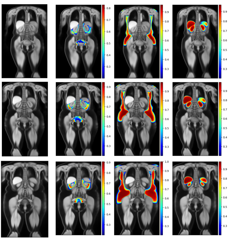
Figure 7: Overview of the female atlases for the healthy (first row), overweight (middle row) and obese (last row) groups.

Male Atlases

Figure 8 shows example slices of the female atlases for each category. The figure shows the water-contrast anatomical atlas side by side with the visceral fat label atlas, the subcutaneous fat label atlas, and the abdominal organs label atlas. Each row corresponds to a different BMI group, from normal (first row) to overweight (middle row) to obese (final row). The colour bar represents the probability of the labels.

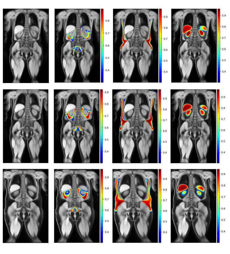
Figure 8: Overview of the male atlases for the healthy (first row), overweight (middle row) and obese (last row) groups.

Distributional Changes in Label Atlases