Geometric Mechanics of Simultaneous Nonslip Contact in a Planar Quadruped

Abstract

In this paper, we develop a geometric framework for generating non-slip quadrupedal two-beat gaits. We consider a four-bar mechanism as a surrogate model for a contact state and develop the geometric tools such as shape-change basis to aid in gait generation, local connection as the matrix-equation of motion, and stratified panels to model net locomotion in line with previous work[1]. Standard two-beat gaits in quadrupedal systems like trot divide the shape space into two equal, decoupled subspaces. The subgaits generated in each subspace space are designed independently and when combined with appropriate phasing generate a two-beat gait where the displacements add up due to the geometric nature of the system. By adding “scaling” and “sliding” control knobs to subgaits defined as flows over the shape-change basis, we continuously steer an arbitrary, planar quadrupedal system. This exhibits translational anisotropy when modulated using the scaling inputs. To characterize the steering induced by sliding inputs, we define an average path curvature function analytically and show that the steering gaits can be generated using a geometric nonslip contact modeling framework.

I Introduction

The framework of geometric mechanics[2] has been used to model a wide class of “geometric” systems– systems with first-order locomotion dynamics fully describable using only the system’s body deformation phase space. The space of all possible body deformations is called the shape space with deformation velocities belonging to its tangent space. The locomotion space is called the position space and has a structure of the Lie group. Based on the locomotion constraint, the ensuing map from the shape velocity to the Lie-algebra of the position space is called the local connection. Furthermore, if one considers periodic body deformation trajectories or periodic gaits in the shape space, a common choice for biological[7] and robotic systems[8, 9], the net displacement of the system can be estimated through the generalized Stokes’ theorem on the local connection[10]. Thus, any quasi-statically locomoting system can be given a geometric description through this framework.

Previous work on quasistatic legged locomotion from a geometric perspective can be divided into three factions. The first faction involves the study of the geometric mechanics of legged systems with a biologically prescribed, a priori contact trajectory[11, 12]. This method provides no analysis of the local connection in each contact state, especially in a average motion-based gait generation (refer to holonomy in [2]) for which the foundations are laid out in this paper. In the second group of work, using nonlinear geometric control theory, Goodwine and Burdick show controllability of drift-free (kinematic) systems living on a discrete set of hierarchically organized kinematic submanifolds called the stratified configuration spaces[13], with a generic recipe for motion planning[14] and quasi-static stability[15] applied to an underactuated hexapod robot model (introduced in[2]). While these control-theoretic findings are informative, they do not shed light on the significance of the robot’s physical characteristics or account for non-standard contact transition assumptions, which hinders their direct applicability to actual robotic systems[16] that can employ diverse foot contact patterns. More recently, Zhao et al.[6] through the generation of data-driven models show that quasistatic legged walking is geometric for a wide range of leg-slipping conditions. Thus, motivated by the above literature and the exciting results from [6], in this work, we explore a first principles-based geometric model of multilegged robots under the no-slip constraint.

Addressing some of these concerns, in our previous work[1] we used a two-footed toy robot model to analyze the simplest instantiation of geometric legged locomotion. Limbs originate from a common hip joint and are constrained to be diametrically opposite to each other. Continuous limb swings and discrete leg contact confers a hybrid shape space to this system. The application generalized Stokes’ theorem for a gait spanning the two contact states– either the left foot or the right foot is in contact, reduces to the difference between the corresponding local connections, called the stratified panel. The stratified panel (a measure of the net displacement accrued through periodic actuation) is then used in an optimal gait generation framework and as a gait coordinate system for the reduction of multi-contact gaits to lower dimensional, two-contact subgaits.

I-A Research Objectives and Contributions

The goal of this letter is to extend our previous work[1] to model the locomotion capabilities of a sprawled, quadrupedal robotic system subject to no-slip contact constraint. To achieve this, a number of key changes have to be made to the two-footed toy model used in our previous work[1]. Firstly, sprawled quadrupedal robots like HAMR[16] have limbs with separate hip joints making it a multi-disk system unlike the single-disk system. Secondly, commonly used two-beat gaits such as trot have two legs on the ground at any given point in time during the gait cycle. Hence, a simple surrogate sub-system describing this contact state would be a three-link system with its distal ends pinned to the ground as shown in Fig.1(a). This is a four-bar mechanism with a single kinematic degree of freedom and a virtual ground link connecting the pinned feet. If a similar simultaneous contact constraint is imposed on the two-footed model from [1], it forms a structure with no degrees of freedom.

With this understanding, the contributions of this paper are summarized below:

• Geometric mechanics of a four-bar mechanism in §II

• Two-beat gait generation for a quadrupedal model in §III

II Geometric Mechanics of planar, four-bar mechanism

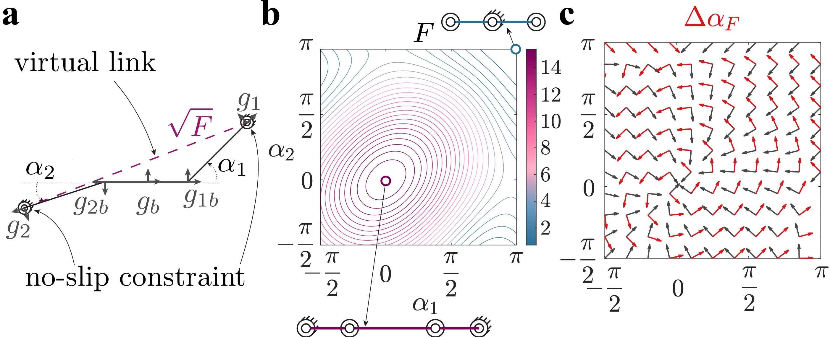
Figure 1: A four-bar mechanism: (a) An illustration of the system is attached $\mathit{SE}(2)$ frames. Because the feet are pinned (extremal points), the virtual link length is a conserved quantity. (b) This quantity is squared ($F$) and plotted as a function of the shape space. Its extrema (inset with configuration) are singular points in the shape space. (c) The derived shape change basis, $\left(\Delta\alpha\right)_{F}$ is plotted on the right, and the red quivers correspond to the no-slip directions tangential to the level-sets of $F$.

As a first step towards describing the geometric mechanics of two-beat quadrupedal gaits, we consider a three-link system with distally pinned feet forming a four-bar mechanism. This system is the simplest instantiation of a no-slip stance phase of a typical two-beat quadrupedal gait and the focus of this section will be the ensuing geometric mechanism of this system.

II-A System Description

Consider the three-link system shown in Fig.1(a). The system has a body link that is two units long and each limb is one unit long. Both limbs have uniform swing angle limits between $-\frac{\pi}{2}$ and $\pi$ radians. Its position is described using $\mathit{SE}(2)$ frames: body center, $g_{b}$, hip joints for each limb, $g_{1b}$ and $g_{2b}$, and foot tips, $g_{1}$ and $g_{2}$. The limb angles for each foot, $\alpha_{i}$, and the binary contact variables, $\beta_{i}$ together form the hybrid shape space of this system. The contact variable sets the current foot to a stance phase if $\beta_{i}=1$ (pinned to the ground[17]) or a swing phase if $\beta_{i}=0$. And, this section is restricted to simultaneous contact of both feet (the $S_{12}$ contact submanifold[1]) in order to aid in the construction and analysis of two-beat gait geometric mechanics in the context of the no-slip locomotion constraint.

II-B No-slip virtual link and singularities

Once both feet are pinned to the ground, the system forms a four-bar mechanism with a virtual link connecting the pinned feet. Following the terminology in [1], we call this contact submanifold $S_{12}$. The virtual link connecting the pinned feet can be written as a transform in the translational sub-space (the rotational component is removed through the use of a selection matrix, $C_{xy}$), $g_{\frac{2}{1}}^{t}$:

$$g_{\frac{2}{1}}^{t}=C_{xy}\,(g_{2}\circ g_{1}^{\hskip 0.3014pt\text{-}1})$$ (1)

$$\text{where }C_{xy}=\begin{bmatrix}1&0&0\\ 0&1&0\end{bmatrix}$$ (2)

Assuming a uniform identity metric over this subspace, the squared length of the virtual link is a scalar field, $F$ in the system’s shape space,

$$F={\left\lVert g_{\frac{2}{1}}^{t}\right\rVert_{2}}^{2}=\left(g_{\frac{2}{1}}^{t}\right)^{T}g_{\frac{2}{1}}^{t}$$ (3)

and is plotted as level-set contours in Fig.1(b).

The extrema of $F$ occurs at two distinct points corresponding to the limbs being parallel (or anti-parallel) to each other. The maximum is attained at $\alpha=(0,0)$, which corresponds to limbs in their 0-position, and the minimum occurs at $(\pi,\pi)$ when the limbs are pointing inwards from their respective hip frames. These configurations (highlighted in Fig.1(b)) are singular since any limb motion results slipping since $F$ changes. Therefore, we compile these extrema into a two-element set of singular configurations, $\tilde{\alpha}$. Hence, an accessible shape space is defined by excluding the singularities: $\alpha_{F}\vcentcolon=\alpha\setminus\tilde{\alpha}$. In the next section, this notion of sticking and slipping is explored more formally in the context of a stick-slip basis for shape velocities.

II-C Stick-slip shape velocity basis

Given an arbitrary limb trajectory, the corresponding trajectory of $F$ reveals the extent to which the system is slipping or sticking. The direction of maximum slippage is given by the gradient, $\nabla F^{T}$ and we call it the slipping direction (this is also scaled by the local value of the gradient). Correspondingly, to compute the sticking direction, we define a clockwise rotational transform, $f_{\epsilon}$ on $\alpha$:

$$f_{\epsilon}:\alpha\longmapsto\alpha\ |\ f_{\epsilon}(\alpha)=\begin{bmatrix}\hphantom{-}\cos{\epsilon}&\sin{\epsilon}\\ -\sin{\epsilon}&\sin{\epsilon}\\ \end{bmatrix}\alpha$$ (4)

The corresponding directional derivative operator, $R$ is obtained by taking the partial derivative with respect to $\epsilon$ at $\epsilon=0$:

$$R=\frac{\partial{f_{\epsilon}(\alpha)}}{\partial{\epsilon}}\bigg{\rvert}_{\epsilon=0}=\begin{bmatrix}\hphantom{-}0&1\\ -1&0\end{bmatrix}$$ (5)

This operator parameterizes an infinitesimal rotation and when applied to $\nabla F^{T}$ provides us with a representation for the sticking direction, $R\nabla F^{T}$. Thus, the stick-slip shape velocity basis, $\Delta\alpha$ (without an explicit parameterization of time) is given by,

$$\Delta\alpha=\begin{bmatrix}R\widehat{\nabla F}^{T}&\widehat{\nabla F}^{T}\end{bmatrix}$$ (6)

where $\widehat{\nabla F}^{T}$ denotes the normalized gradient, and when taken together with $R\widehat{\nabla F}^{T}$ provides an orthonormal basis for shape changes, $\Delta\alpha$. For the system parameters considered in §II-A, the virtual-link transform and its squared length are computed below:

$$g_{\frac{2}{1}}^{t}=\begin{bmatrix}\cos\alpha_{2}-\cos\alpha_{1}-2\\ \sin\alpha_{2}-\sin\alpha_{1}\end{bmatrix}$$ (7)

$$F={{\left(\cos\alpha_{1}-\cos\alpha_{2}+2\right)}}^{2}+{{\left(\sin\alpha_{1}-\sin\alpha_{2}\right)}}^{2}$$ (8)

The contours of $F$ shown above are plotted as a function of the shape space in Fig.1(b). Then, substituting (8) in (6), we obtain the stick-slip shape velocity basis. The sticking directions are depicted with red quivers and the slipping directions are depicted with gray quivers in Fig.1(c). Note that, at the singularities, the gradient is a zero vector (thus, the basis is undefined), and all shape changes here involve slipping because we are moving away from the extrema.

II-D Path description

Consider an arbitrary, time-parameterized, continuous trajectory in the shape space, $\alpha(t)\in\alpha_{F},\,\,t\in[t_{0},t_{f}]$.

$$\alpha(t)=\int_{t_{0}}^{t}\dot{\alpha}(\tau)\,d\tau+\alpha(t_{0}),$$ (9)

where $\alpha(t_{0})$ is the initial shape. Substituting (6) in (9), and simplifying, we have:

$$\alpha(t)=\int_{t_{0}}^{t}(\Delta\alpha)\,\dot{k}\,d\tau+\alpha(t_{0})$$ (10)

where $\dot{k}$ represents the velocity in the stick-slip coordinates. The first component, $\dot{k}_{1}$ encodes the velocity projection in the stick direction, whereas the second component, $\dot{k}_{2}$ encodes the velocity projection in the slip direction.

The validity of the no-slip constraint in predicting motion induced by slipping limbs warrants a separate investigation and is outside the scope of this paper. Therefore, for the methods developed in this paper, we consider continuous limb trajectories without slip that evolve on levels of $F$:

$$\alpha(t)=\int_{t_{0}}^{t}R\widehat{\nabla F}\,\dot{k}\,d\tau+\alpha(t_{0}),\,\dot{k}\in\mathbb{R}$$ (11)

where $\dot{k}$ is redefined as a scalar, pacing term for paths evolving on level-sets of $F$. And finally, we define the set accessible shape velocities, $\Delta\alpha_{F}$ in the tangent bundle of the accessible shape space, $T{\alpha}_{F}$ as follows:

$$\Delta\alpha_{F}=R\widehat{\nabla F}(\alpha),\,\,\alpha\in\alpha_{F}$$ (12)

Thus, (11) and (12) help us define paths in the shape space that prevent the feet from slipping. Using flow notation, (11) can be written as follows:

$$\alpha(t)=\Phi_{\Delta\alpha_{F}\,\dot{k}}^{t}(\alpha(t_{0}))$$ (13)

where, $\Phi_{\Delta\alpha_{F}\,\dot{k}}^{t}(\alpha(t_{0}))$ denotes flow along the vector field $\Delta\alpha_{F}$ with for time $t$ from $\alpha(t_{0})$.

II-E Kinematic Reconstruction using the No-slip constraint

Figure 2: Geometric mechanics of a four-bar mechanism: (a) The local connection vector fields $\vec{\mathbf{A}}$ model the kinematics of the four-bar mechanism. (b) The stratified panel, $dz$ is a visual gait generation tool from which the net displacement can be estimated. In (c) and (d), the stance phase path in an example gait $\phi$ and the corresponding $\mathit{SE}(2)$ body trajectory of the system are shown in red.

The equations of motion of the four-bar system can be written using linear constraints in its body frame. As shown previously[1], we find the jacobians that transform the system’s generalized velocity (the body velocity, $\mathchoice{\accentset{\scriptstyle\circ}{g}}{\accentset{\scriptstyle\circ}{g}}{\accentset{\scriptscriptstyle\circ}{g}}{\accentset{\scriptscriptstyle\circ}{g}}_{b}$ and leg-swing velocity, $\dot{\alpha}$) to the local foot velocity, $\mathchoice{\accentset{\scriptstyle\circ}{g}}{\accentset{\scriptstyle\circ}{g}}{\accentset{\scriptscriptstyle\circ}{g}}{\accentset{\scriptscriptstyle\circ}{g}}_{i}$. The jacobians for each foot are given below:

$$J_{1}=\begin{bmatrix}\hphantom{-}\cos\alpha_{1}&\sin\alpha_{1}&\sin\alpha_{1}&0&0\\ -\sin\alpha_{1}&\cos\alpha_{1}&\cos\alpha_{1}+1&1&0\\ 0&0&1&1&0\end{bmatrix}$$ (14)

$$J_{2}=\begin{bmatrix}\hphantom{-}\cos\alpha_{2}&\sin\alpha_{2}&-\sin\alpha_{2}&0&0\\ -\sin\alpha_{2}&\cos\alpha_{2}&1-\cos\alpha_{2}&0&1\\ 0&0&1&0&1\end{bmatrix}$$ (15)

Next, we impose the no-slip constraint as zero translational velocity for each foot and concatenate the two resulting constraints into a single pfaffian constraint expression:

$$\begin{bmatrix}C_{xy}J_{1}\\ C_{xy}J_{2}\end{bmatrix}\begin{bmatrix}\mathchoice{\accentset{\scriptstyle\circ}{g}}{\accentset{\scriptstyle\circ}{g}}{\accentset{\scriptscriptstyle\circ}{g}}{\accentset{\scriptscriptstyle\circ}{g}}_{b}\vspace{1mm}\\ \dot{\alpha}\end{bmatrix}=\left(0\right)^{4\times 1}$$ (16)

For an arbitrary m-legged stance phase of a planar, n-legged system (with $m\leq n$ obviously), the no-slip pfaffian constraint can be written as:

$$\begin{bmatrix}\vdots\\ C_{xy}J_{i}\\ \vdots\end{bmatrix}^{2m\times(n+3)}\begin{bmatrix}\mathchoice{\accentset{\scriptstyle\circ}{g}}{\accentset{\scriptstyle\circ}{g}}{\accentset{\scriptscriptstyle\circ}{g}}{\accentset{\scriptscriptstyle\circ}{g}}_{b}\vspace{1mm}\\ \dot{\alpha}\end{bmatrix}^{(n+3)\times 1}=\left(0\right)^{2m\times 1}$$ (17)

Finally, dividing (16) into two sub-matrices and then taking the pseudoinverse as instructed in [10], we obtain the local connection vector field, $\mathbf{A}_{12}$– a map from the shape velocities to the body velocity, $\mathchoice{\accentset{\scriptstyle\circ}{g}}{\accentset{\scriptstyle\circ}{g}}{\accentset{\scriptscriptstyle\circ}{g}}{\accentset{\scriptscriptstyle\circ}{g}}_{b}=-\mathbf{A}_{12}\dot{\alpha}$. This equation is known as the kinematic reconstruction. The local connection matrix has two columns each corresponding to the body velocity contribution from each shape element velocity. It has three rows in total corresponding to the $\mathit{SE}(2)$ directions– $(x,y,\theta)$. Thus, each row called the connection vector field is plotted as a function of the shape space in Fig.2(a). If the shape velocity is aligned along the quivers, then a positive body velocity is generated in the corresponding direction.

The connection vector fields developed in §II-E are conservative for all nonslip limb actuation as defined in (11). This implies two things:

1. A closed-loop, nonslip path in the shape space with just a stance phase $S_{12}$ does not generate any net displacement. Thus, any gait in the shape space needs to span multiple contact submanifolds to generate a net displacement.

2. The net displacement generated is pacing independent– meaning, due to the conservative nature of the system, only the final and initial points matter, and the exact velocity information at a certain point along the shape path is irrelevant for the net $\mathit{SE}(2)$ displacement generated by the system.

II-F Gait Description

Consider the gait $\phi$ in the shape space shown in Fig.1(f). The gait phase variable, $\tau\in\mathbb{S}^{1}$ is used to parameterize the current phase of the gait cycle and a discrete foot contact variable, $\beta$ parameterizes the contact state. Let us define the shapes at any $\tau$ as $\alpha_{\tau}$– thus, at $\tau=0$ and $\tau=\pi$ the shapes are $\alpha_{0}$ and $\alpha_{\pi}$ as shown in the figure. During the first half of the gait cycle, $[0,\pi)$ the forward path is executed and is shown with a red trace to denote the stance phase, $\beta=1$ or $S_{12}$ contact submanifold. During the second half of the gait cycle, $[\pi,2\pi)$ the return path retraces the forward path and returns to the initial condition through the swing phase, $\beta=0$ or $S_{\emptyset}$. Using (13), the gait cycle $\phi$ can be succinctly represented using flow notation:

$$\phi_{\tau}=\begin{bmatrix}\alpha\\ \beta\end{bmatrix}_{\tau}=\begin{cases}\begin{bmatrix}\Phi_{\Delta\alpha_{F}\,\dot{k}}^{\tau}(\alpha_{0})\\ 1\end{bmatrix},\>\>0\leq\tau<\pi\\ \begin{bmatrix}\Phi_{\Delta\alpha_{F}\,\dot{k}}^{\pi-\tau}(\alpha_{\pi})\\ 0\end{bmatrix},\>\>\pi\leq\tau<2\pi\end{cases}$$ (18)

In (18), $\alpha_{\pi}=\Phi_{\Delta\alpha_{F}}^{t(\pi)}(\alpha_{0})$ and $\Phi_{-\Delta\alpha_{F}}^{t(\tau-\pi)}$ each correspond to the flow that generates the shape trajectory during the stance phase and swing phase respectively. If the desired path length is $t$ in each contact phase (in such a case, the total path length of gait $\phi$ adds up to $2t$), then the required constant pacing is:

$$\dot{k}=\frac{t}{\pi}$$ (19)

The corresponding trajectory of the system (or the body frame), $g_{b}(\tau)$ can be written in flow notation and is obtained by integrating the pullback of the body velocity to the rest frame, $T_{e}{L}_{g_{b}}$ (shown as $g$ for brevity):

$$\dot{g}_{b}(\tau) =-g\,\mathchoice{\accentset{\scriptstyle\circ}{g}}{\accentset{\scriptstyle\circ}{g}}{\accentset{\scriptscriptstyle\circ}{g}}{\accentset{\scriptscriptstyle\circ}{g}}_{b}=-g\mathbf{A}\,\Delta\alpha_{F}\dot{k}$$ (20)

$$g_{b}(\tau) =\begin{cases}\Phi_{\dot{g}_{b}(\tau)}^{\tau}(\,g_{b}(0)\,),\>\>\tau<\pi\\ g_{b}(\pi),\>\>\pi\leq\tau<2\pi\end{cases}$$ (21)

During $S_{\emptyset}$, no motion is generated due to the absence of contact and thus the body frame remains unchanged.

II-G Stratified Panel

The net displacement, $z_{\phi}$ for the gait cycle, $\phi$ considered in (18) can be obtained by closed integration of the body velocity from the perspective of the rest frame using (11) as follows:

$$z_{\phi}=\ointctrclockwise_{\phi}-g(\mathbf{A}\Delta\alpha_{F}\dot{k})(\phi)=g_{b}(2\pi)$$ (22)

This integral can be divided into a separate integral in each contact phase and the $\tau$-dependence can be removed by moving the integral to the shape space coordinates. Then, using the fact that no motion is generated during the swing phase (21), the above expression is simplified to:

$$z_{\phi}=\int_{\alpha_{0}}^{\alpha_{\pi}}-g\mathbf{A}_{12}\Delta\alpha_{F}\,dk$$ (23)

The quantity, $\mathbf{A}_{12}\Delta\alpha_{F}$ is called the stratified panel, $dz$. The effective body velocity for the infinitesimal gait centered around $\alpha$ is the stratified panel $dz(\alpha)$. This velocity times the infinitesimal limb swing $dk$ provides the net displacement accrued by the infinitesimal gait. Pulling the local body velocity ($\mathbf{A}_{12}\Delta\alpha_{F}dk$) to the rest frame and integrating as shown in (23) provides the net displacement of the complete gait. The stratified panels are plotted as a scalar field of the shape space in Fig.1(e).

II-H Translational Gait design

The rotational subgroup $\mathit{SO}(2)$ of the semidirect product group $\mathit{SE}(2)$ (our space of rigid-body planar motions) is an abelian (commutative) subgroup. This means that the yaw panels give an exact representation of the effective rotational velocity generated over a gait cycle, and together with the skew-symmetry exhibited by this panel about the $\alpha_{1}=\alpha_{2}$ line (also the zero contour line of this panel), we gain the ability to generate gaits that only produce a net translation or translational gaits. In a translational gait, the path in both the stance and the swing phases is centered on the $\alpha_{1}=\alpha_{2}$ line to take advantage of the skew-symmetry property and the abelian nature of the yaw panels. The procedure to generate such a gait is outlined below:

1. To create a translation gait we need the path to be centered about the $\alpha_{1}=\alpha_{2}$ line. Therefore, we choose a point of interest $\alpha_{*}$ along the $\alpha_{1}=\alpha_{2}$ line to choose $F$-level to operate in. Note that the chosen $F$-level determines the shapes accessible during the gait cycle.

2. Next, the initial condition $\alpha_{0}$ and a path length $t$ are required to construct the path during each contact phase. Flowing from the point of interest with unit pacing, the initial condition is given by,

   $$\alpha_{0}=\Phi_{\Delta\alpha_{F}}^{\pm\frac{t}{2}}(\alpha_{*})$$ (24)

   To compute the endpoint of the stance phase $\alpha_{\pi}$, the direction of the previous flow (24) is reversed:

   $$\alpha_{\pi}=\Phi_{\Delta\alpha_{F}}^{\mp\frac{t}{2}}(\alpha_{*})$$ (25)

The path lengths to the initial and final points of the stance phase from the point of interest is uniquely identified above using flow times, $t_{0}=\frac{t}{2}$ and $t_{\pi}=-\frac{t}{2}$. Combining the above results with (18) and (19) provides a recipe for constructing translation gaits as used in the example shown in Fig.2 where the point of interest is $(\frac{\pi}{4},\frac{\pi}{4})$ and the total path length is $t_{0}+t_{\pi}=2$ in each contact phase.

More generally, using function notation we represent an arbitrary gait $\phi$ as follows:

$$\phi(\tau;\alpha_{*},t_{0},t_{\pi})$$ (26)

This gait function (26) is defined with respect to the gait phase variable, and the parameters defining the starting and the ending point are collected after the semi-colon. Note that if the path has to be centered about the point of interest, then the flow times need to have the same magnitude but opposing signs as shown in (24) and (25).

III Two-beat gait generation for a rigid quadrupedal system

This section uses the tools developed in §II to generate a trot gait for an arbitrary quadrupedal model.

III-A Planar quadrupedal system

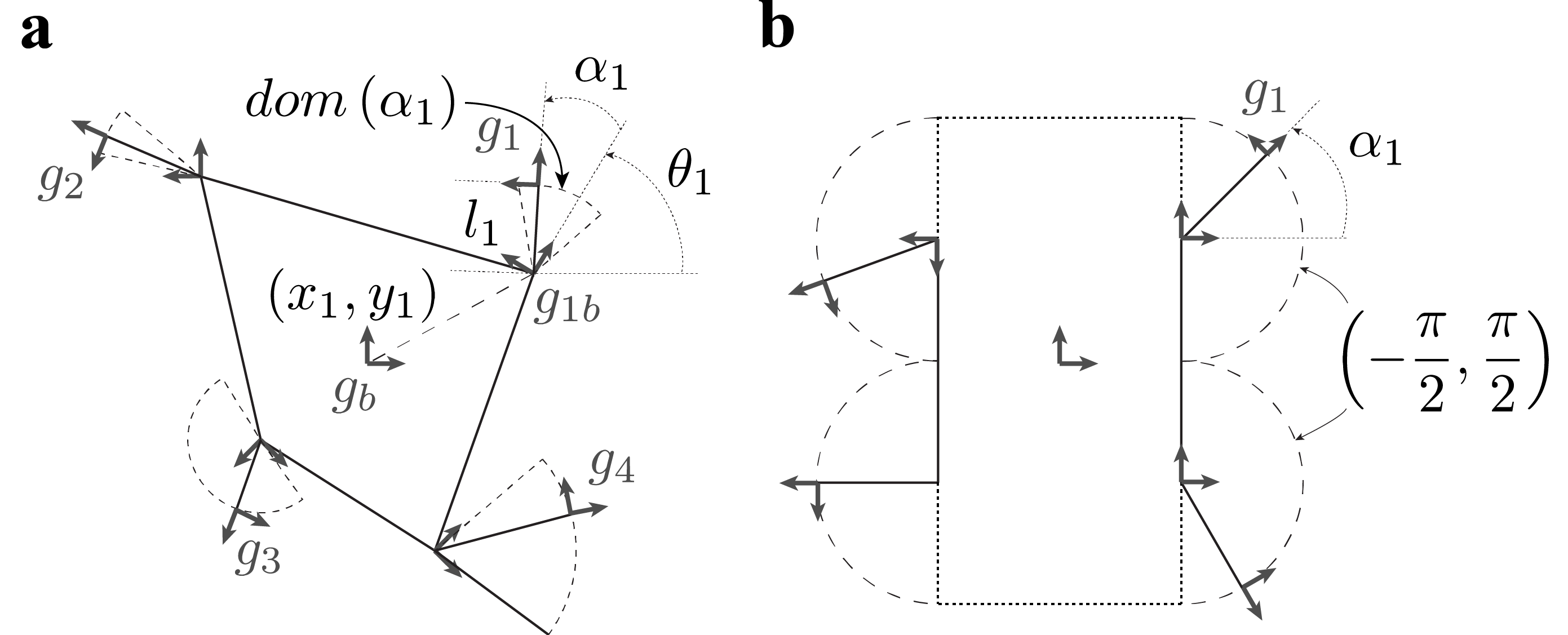
Figure 3: An arbitrary, planar quadrupedal system in (a) is defined using parameters for each leg module. By choosing a unit offsets from the body frame to each hip frame and unit leg length with a swing domain of $(-\frac{\pi}{2},\frac{\pi}{2})$, we obtain the quadrupedal system (b) used in §III.

Consider an arbitrary quadrupedal system shown in Fig.3(a). The foot position of the i^th leg module in this system is defined by the location of the hip joint ($g_{ib}$ frame), the leg length ($l_{i}$), the swing angle ($\alpha_{i}$), and the current leg contact state ($\beta_{i}$). In Fig.3(b) we define the above quantities for each leg module and obtain a description of the planar HAMR-VI model. The body of this sprawled robot is symmetric about both body axes with a $90^{\circ}$, bidirectional swing range.

III-B Geometric nonslip trot gait

III-B1 Definition

The hybrid shape space of the planar HAMR model is an extension of the system in §II. The shape space of the system is parameterized by four continuous swing angle shapes and four discrete lift shapes. So, there are six distinct ways of stancing two legs with the contact submanifolds being $S_{12}$, $S_{23}$, $S_{34}$, $S_{41}$, $S_{13}$, and $S_{24}$. For a trot gait, the contact trajectory involves alternating between the stance phases of the diagonally opposite legs, and similarly, in a bound gait, the contact trajectory of the system alternates between the stance phases of the front and hind legs. Based on the contact trajectory, the paths taken by each stance phase pair are decoupled from each other, dividing shape space into two equal halves. Therefore, a trot gait trajectory defined over a gait phase variable $\tau$ is broken down into two subgaits each spanning a different shape sub-space:

$$\phi_{13\leftrightarrow 24}(\tau) =\hat{\phi}_{13}(\tau)+\hat{\phi}_{24}(\pi+\tau)$$ (27)

$$z_{\phi} =z(\hat{\phi}_{13})+z(\hat{\phi}_{24})$$ (28)

In (27), $\hat{\phi}_{12}$ and $\hat{\phi}_{24}$ are the subgaits that form a gait coordinate system to uniquely define trot gaits $\phi_{13\leftrightarrow 24}$ defined as periodic shape trajectories. The uniqueness of this definition is a result of the subgaits residing in decoupled shape subspaces. The subgaits are defined using (18), and the stance phases are offset by $\pi$ to prevent overlap. The net displacement generated by this gait is the sum of the displacements generated by each sub-gait as shown in (28). This key result helps us steer the subgaits independently to achieved a desired geometric trotting behavior.

III-B2 Translational trotting

We use the same strategy described in §II-H to create a net forward displacing trot gait with identically parameterized subgaits. These subgaits are embedded on the stratified panels of their respective subspaces in Fig.4(b) and (c). With the origin as the point of interest, they both use flow times $t_{0}=0.8$ and $t_{\pi}=-0.8$, resulting in a stance paths with a clockwise (negative) sense around the singularity and thus, negate the effective velocity predicted by the panels. The $x$-panels also have inverted structure in each contact state as a result of the left-right body symmetry and thus, cancel the lateral displacements generated in each gait cycle.

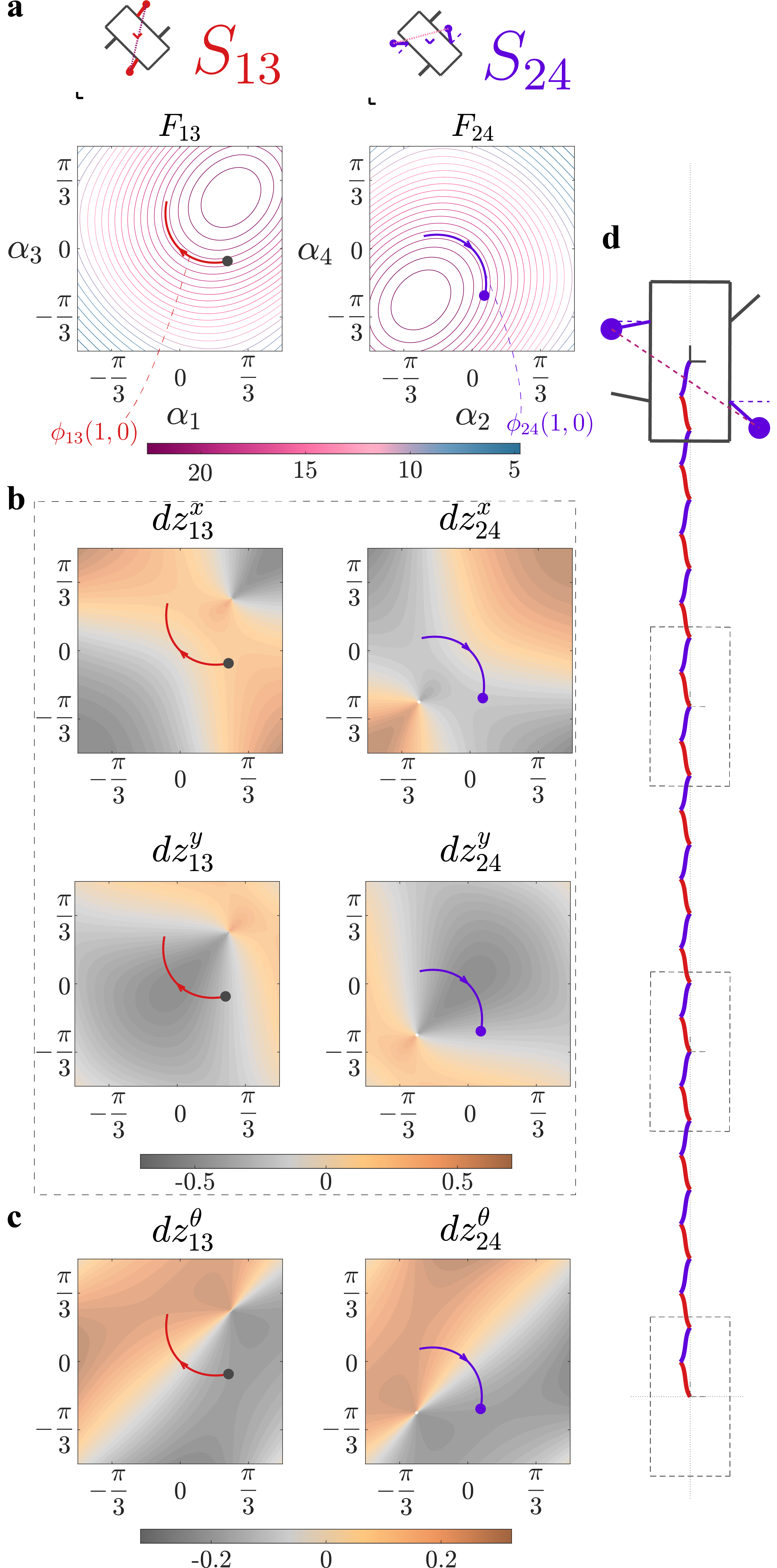
Figure 4: A forward displacing trot gait generated by subgaits in $S_{13}$ and $S_{24}$. (a) The level-sets of of each shape subspace help in gait change basis construction. (b) The translational and (c) rotational panels of the two contact states are shown. An example gait is embedded in the above shape subspaces and is run for 15 gait cycles for which body trajectory is shown in (d).

III-C Flow-control of subgaits

Directly tuning three parameters of each subgait flow to obtain a desired geometric trotting behavior is tedious. Therefore, in this section we introduce two different kinds of control knobs to intuitively generate subgaits that serve a specific purpose.

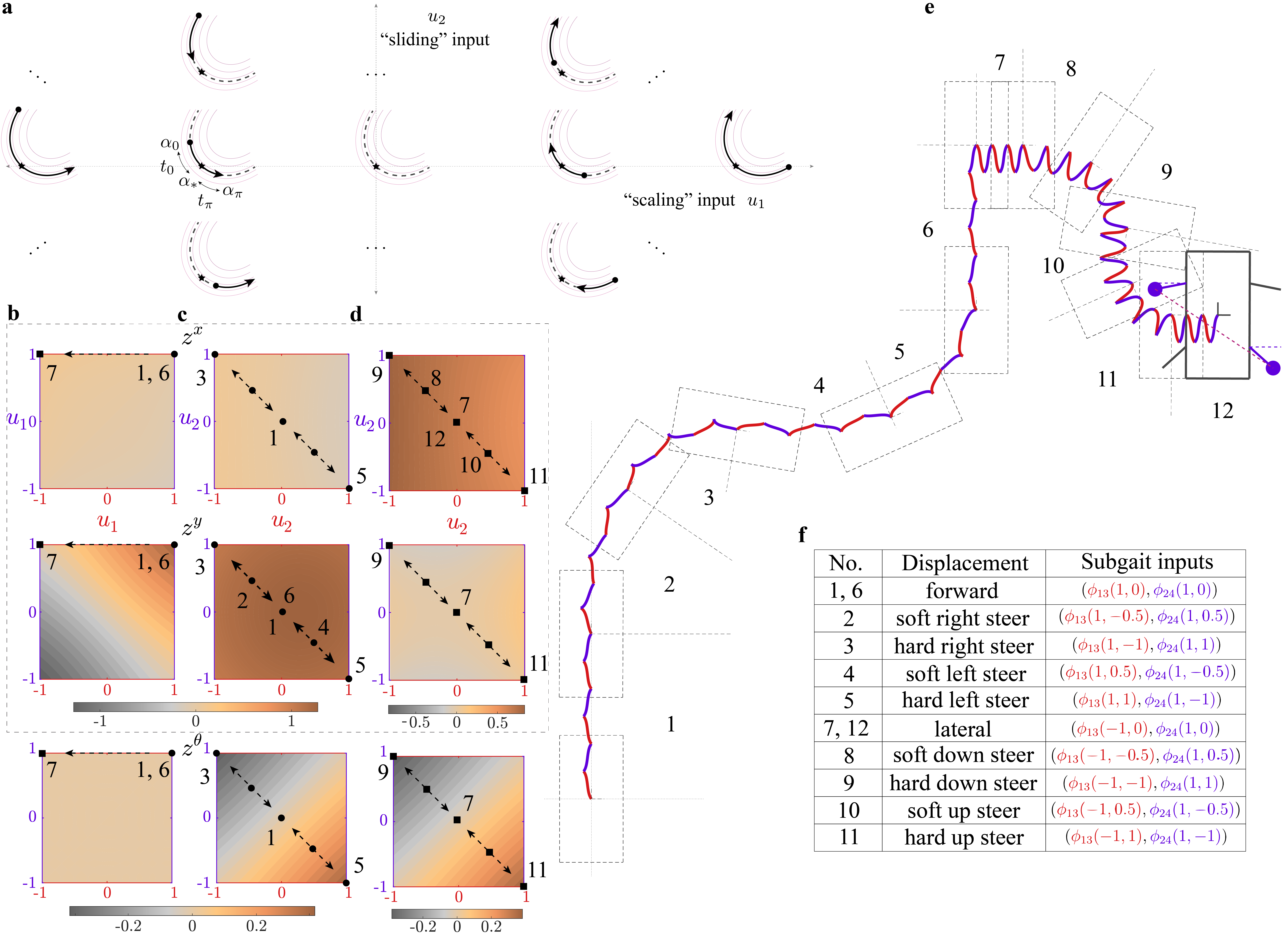
Figure 5: Overview of steerable geometric trot gait design: (a) Subgait flow control: To parameterize the stance phase path of a subgait, we require the point of interest $\alpha_{*}$, the initial and final conditions $\alpha_{0}$ and $\alpha_{\pi}$, the path lengths to both points $t_{0}$ and $t_{\pi}$, and inputs $u_{1}$ and $u_{2}$. Thus, the two inputs for a two-parameter family of periodic sub-gaits. (b) The net displacement is plotted as a heatmap in the scaling input– $x$-axis encodes the scaling of $\phi_{13}$ and the $y$-axis encodes the scaling of $\phi_{24}$. The trajectories $1$, $6$, and $7$ correspond to the translational gaits used in the composite trajectory. (c) and (d) show the net displacement generated as a function of the sliding input space as perturbations on the translational gaits (residing in the origin of this space). The forward steering gaits from $2$ through $5$, and the lateral steering gaits from $8$ through $11$ are shown in their respective spaces. (e) The position trajectory of the system is shown as with the body orientation shown after every gait sequence set. Each gait used in this sequence is listed in the table inset (f) with a description, parameter input, and the net path curvature generated.

III-C1 Scaling flow input

The scaling flow control amplifies the path length of the subgait using the flow times from the point of interest. Incorporating the scaling input $u_{1}$ into (24) and (25) with generic parameters, we have:

$$\alpha_{0}=\Phi_{\Delta\alpha_{F}}^{u_{1}t_{0}}(\alpha_{*})$$ (29)

$$\alpha_{\pi}=\Phi_{\Delta\alpha_{F}}^{-u_{1}t_{\pi}}(\alpha_{*})$$ (30)

The impact of the scaling inputs on subgaits are depicted along the $x$-axis in Fig.5. The scaling inputs scale paths uniformly about the point of interest. At $u_{1}=0$, both flow times are zero rendering a subgait with no pathlength and displacement. For positive values of $u_{1}$, the path length increases while maintaining the direction defined by the flow times. Similarly, for negative values of $u_{1}$, the path length increases, but the direction is flipped. The scaling input preserves the . The translational gait shown in Fig.4 can be represented with unity scaling inputs and the parameters defined in §III-B2.

III-C2 Sliding flow input

In [6], the authors define steering as the ability to continuously select the rotational component of the net displacement generated by a gait with a single parameter. This provides the key motivation for a “sliding” flow control parameter provided here. This parameter “slides” the path relative to the point of interest (along the current level-set of F) by inducing a net-shift in the flow times.

Consider stance phase of each subgait embedded on the $\theta$-panels in Fig.4. The net rotation generated by the subgaits in the first half of the stance phase is cancelled by the rotation induced in the second half. This balance in rotation is perturbed by the sliding control parameter and its effect on the subgait is illustrated along the $y$-axis in Fig.5. Incorporating this input as well into (29) and (30), the initial and final conditions of the stance phase path are given by:

$$\alpha_{0}=\Phi_{\Delta\alpha_{F}}^{u_{1}t_{0}+u_{2}}(\alpha_{*})$$ (31)

$$\alpha_{\pi}=\Phi_{\Delta\alpha_{F}}^{-u_{1}t_{\pi}+u_{2}}(\alpha_{*})$$ (32)

Notice how the addition of $u_{2}$ to flow times generates a affine, directional shift in both the initial and final conditions– the direction of the shift is determined by its sign. While sliding the path, the input preserves its length.

III-D Steerable trajectories

The net displacements generated by the two subgait, two-parameter families resulting in a geometric nonslip trot gait are hard to visualize because displacement fields are four dimensional. Therefore, to help generate gaits and visualize the impact of flow control knobs, we have designed a composite gait trajectory as a perturbation on the forward displacing trot gait generated in §III-B2.

The first half of the composite trajectory starts off with a forward displacement trot gait ($1$) for three gait cycles, followed three gait cycles of a soft ($2$) and hard right ($3$) steered gaits, then by three gait cycles of soft ($4$) and hard left ($5$) steered gaits, and a final three cycles of the forward gait ($6$). The net displacement generated by by this sequence of longitudinally steered gaits are shown in Fig.5(b) and (c), and the position trajectory is shown in (e). Alternating between left and right steered gaits generates a serpenoid motion in the locomotion plane.

The second half starts off with a lateral displacement trot gait ($7$) obtained by changing scaling parameter of $\phi_{13}$ from $1$ to $-1$, thus flipping the direction of the stance path. This results in a rightward shuffle-like translation gait. The displacement heatmap in Fig.5(b) shows the anisotropy in the ability to generate translation by modulating scaling inputs. A rigid-bodied, planar quadrupedal robot with lateral limb orinetation generates greater longitudinal displacement than lateral displacement.

Following the lateral gait ($7$), a sequence of laterally steered gait– left steered gaits (soft $8$, hard $9$) and right steered gaits (soft $10$, hard $11$) are implemented. The net displacement generated by these gaits are shown in Fig.5(c) and (d). They produces a serpenoid motion similar to the longitudinal sequence from the first half, but have diminished displacement due to the translational anisotropy.

For both longitudinal or lateral steering in the corresponding sliding input spaces, the displacement fields show $y$ or $x$-displacement with continuously modulatable rotational displacement along the $\left(u_{13}\right)_{2}=-\left(u_{24}\right)_{2}$ line. This directly represents the steering gaits defined in [6]– where using these fields we have a continuous choice over the rotational displacement generated by these gaits.

Another useful formulation for steering gaits is through the average curvature of the position trajectory. For a time-parameterized path through the locomotion plane, $(x(t),y(t))$, the signed curvature of the path $k(t)$ is given by:

$$k=\frac{\dot{x}\ddot{y}-\dot{y}\ddot{x}}{\left({\dot{x}}^{2}+{\dot{y}}^{2}\right)^{\frac{3}{2}}}$$ (33)

This equation (33) can be rewritten as the average path curvature of a gait cycle, $\bar{k}(\phi)$ using the system’s velocity $\dot{g}$ and acceleration $\ddot{g}$ with respect to a rest frame as follows:

$$\bar{k}(\phi)=\frac{1}{2\pi}\ointctrclockwise_{\phi}\frac{\dot{g}^{x}\ddot{g}^{y}-\dot{g}^{y}\ddot{g}^{x}}{{\left\lVert C_{xy}\dot{g}\right\rVert_{2}}^{3}}$$ (34)

In (34), the acceleration of the body velocity is computed by taking the derivative of the body velocity (20):

$$\ddot{g}=-\dot{g}^{\theta}\frac{\partial T_{e}{L}_{g_{b}}}{\partial\theta}\mathbf{A}\dot{\alpha}- T_{e}{L}_{g_{b}}\left[\ldots\>\nabla_{\alpha}\mathbf{A}_{i}\dot{\alpha}\>\ldots\right]\dot{\alpha}$$

$$- T_{e}{L}_{g_{b}}\mathbf{A}\ddot{\alpha}$$ (35)

The three terms from left to right in the above equation encode the effect of the pullback’s derivative, the local connection’s derivative, and the shape acceleration. Therefore using (34) and (35), the average curvature generated by the steering gaits are shown in Fig.5(f) table inset.

IV Discussion

In §II, we studied a four-bar mechanism that represents a generic contact state (stance phase) in a quadrupedal two-beat gait cycle. This mechanism consists of three links with extremal points pinned together. However, arbitrary motions in the shape-space can cause slipping. Thus, we create a nonslip shape velocity basis using the conserved quantity of squared inter-leg distance during the stance phase.

We then determined the Pfaffian constraint that describes simultaneous non-slip contact. By pseudoinverting the submatrices, we obtained the local connection, $\mathbf{A}$, a first-order shape-defined matrix equation of motion that maps our shape velocity to the local body velocity of the system– in other words, a map to the velocity of the middle link given the joint velocities of the distal links. Finally, we used the local connection and the shape velocity basis over a gait cycle to obtain the description of a stratified panel that measures the effective body velocity generated by an infinitesimal, discretely contact-switching gait cycle. In this work, to describe this panel, we use the complementary approach of the boundary integral in comparison to previous work[1] where the generalized Stokes’ theorem was used. Finally, using the fact that the rotational motion is commutative and the skew-symmetry of the yaw panel, we develop a flow-based framework for translational gait generation.

In §III, we showed that in a typically two-beat gait cycle such as trot the shape space of the system gets split into two halves with decoupled subgaits. This means that subgaits can be generated in isolation and can be added again with appropriate phase offset to obtain the trot gait. Because of the geometric nature of the locomotion, the net displacements by the sub-gaits added up to obtain the net displacement of the trot gait.

Then, to modulate the trotting behavior and generate steering trot gaits, we introduce two kinds of flow control inputs– the scaling input and sliding input. Modulating the scaling input led to translation gaits generating net displacement in all directions of the locomotion plane with anisotropy, but strongest and weakest displacement directions were aligned longitudinally and laterally. Modulating sliding inputs resulted in shifting the delicate balance of cancelling net rotation in each contact state. Thus, this input was responsible in the generation of steering gaits with continuous steering in a closed interval around zero. At the end of this section, we gave steering gaits another meaning by developing a representation for average path curvature as a function of the body trajectory.

References

- [1] H. K. H. Prasad, R. L. Hatton, and K. Jayaram, “Geometric mechanics of contact-switching systems,” arXiv preprint arXiv:2306.10276, 2023.
- [2] S. D. Kelly and R. M. Murray, “Geometric phases and robotic locomotion,” Journal of Robotic Systems, vol. 12, no. 6, pp. 417–431, 1995.
- [3] R. L. Hatton, Z. Brock, S. Chen, H. Choset, H. Faraji, R. Fu, N. Justus, and S. Ramasamy, “The geometry of optimal gaits for inertia-dominated kinematic systems,” IEEE Transactions on Robotics, vol. 38, no. 5, pp. 3279–3299, 2022.
- [4] C. Li, T. Zhang, and D. I. Goldman, “A terradynamics of legged locomotion on granular media,” science, vol. 339, no. 6126, pp. 1408–1412, 2013.
- [5] R. L. Hatton and H. Choset, “Geometric swimming at low and high reynolds numbers,” IEEE Transactions on Robotics, vol. 29, no. 3, pp. 615–624, 2013.
- [6] D. Zhao and S. Revzen, “Multi-legged steering and slipping with low dof hexapod robots,” Bioinspiration & biomimetics, vol. 15, no. 4, p. 045001, 2020.
- [7] Y. O. Aydin, B. Chong, C. Gong, J. M. Rieser, J. W. Rankin, K. Michel, A. G. Nicieza, J. Hutchinson, H. Choset, and D. I. Goldman, “Geometric mechanics applied to tetrapod locomotion on granular media,” in Conference on Biomimetic and Biohybrid Systems. Springer, 2017, pp. 595–603.
- [8] B. A. Bittner, R. L. Hatton, and S. Revzen, “Data-driven geometric system identification for shape-underactuated dissipative systems,” Bioinspiration & biomimetics, 2021.
- [9] B. Chong, J. He, D. Soto, T. Wang, D. Irvine, G. Blekherman, and D. I. Goldman, “Multilegged matter transport: A framework for locomotion on noisy landscapes,” Science, vol. 380, no. 6644, pp. 509–515, 2023.
- [10] R. L. Hatton and H. Choset, “Nonconservativity and noncommutativity in locomotion,” The European Physical Journal Special Topics, vol. 224, no. 17, pp. 3141–3174, 2015.
- [11] B. Chong, Y. O. Aydin, C. Gong, G. Sartoretti, Y. Wu, J. M. Rieser, H. Xing, P. E. Schiebel, J. W. Rankin, K. B. Michel, et al., “Coordination of lateral body bending and leg movements for sprawled posture quadrupedal locomotion,” The International Journal of Robotics Research, vol. 40, no. 4-5, pp. 747–763, 2021.
- [12] B. Chong, J. He, S. Li, E. Erickson, K. Diaz, T. Wang, D. Soto, and D. I. Goldman, “Self-propulsion via slipping: Frictional swimming in multilegged locomotors,” Proceedings of the National Academy of Sciences, vol. 120, no. 11, p. e2213698120, 2023.
- [13] B. Goodwine and J. W. Burdick, “Controllability of kinematic control systems on stratified configuration spaces,” IEEE Transactions on Automatic Control, vol. 46, no. 3, pp. 358–368, 2001.
- [14] J. Burdick and B. Goodwine, “Quasi-static legged locomotors as nonholonomic systems,” in Proceedings. 2000 IEEE/RSJ International Conference on Intelligent Robots and Systems (IROS 2000)(Cat. No. 00CH37113), vol. 1. IEEE, 2000, pp. 817–825.
- [15] B. Goodwine and J. W. Burdick, “Motion planning for kinematic stratified systems with application to quasi-static legged locomotion and finger gaiting,” IEEE Transactions on robotics and automation, vol. 18, no. 2, pp. 209–222, 2002.
- [16] S. D. De Rivaz, B. Goldberg, N. Doshi, K. Jayaram, J. Zhou, and R. J. Wood, “Inverted and vertical climbing of a quadrupedal microrobot using electroadhesion,” Science Robotics, vol. 3, no. 25, p. eaau3038, 2018.
- [17] A. Ruina, “Nonholonomic stability aspects of piecewise holonomic systems,” Reports on mathematical physics, vol. 42, no. 1-2, pp. 91–100, 1998.
- [18] S. Ramasamy and R. L. Hatton, “The geometry of optimal gaits for drag-dominated kinematic systems,” IEEE Transactions on Robotics, vol. 35, no. 4, pp. 1014–1033, 2019.