TransGNN: Harnessing the Collaborative Power of Transformers and Graph Neural Networks for Recommender Systems

Abstract.

Graph Neural Networks (GNNs) have emerged as promising solutions for collaborative filtering (CF) through the modeling of user-item interaction graphs. The nucleus of existing GNN-based recommender systems involves recursive message passing along user-item interaction edges to refine encoded embeddings. Despite their demonstrated effectiveness, current GNN-based methods encounter challenges of limited receptive fields and the presence of noisy “interest-irrelevant” connections. In contrast, Transformer-based methods excel in aggregating information adaptively and globally. Nevertheless, their application to large-scale interaction graphs is hindered by inherent complexities and challenges in capturing intricate, entangled structural information. In this paper, we propose TransGNN, a novel model that integrates Transformer and GNN layers in an alternating fashion to mutually enhance their capabilities. Specifically, TransGNN leverages Transformer layers to broaden the receptive field and disentangle information aggregation from edges, which aggregates information from more relevant nodes, thereby enhancing the message passing of GNNs. Additionally, to capture graph structure information effectively, positional encoding is meticulously designed and integrated into GNN layers to encode such structural knowledge into node attributes, thus enhancing the Transformer’s performance on graphs. Efficiency considerations are also alleviated by proposing the sampling of the most relevant nodes for the Transformer, along with two efficient sample update strategies to reduce complexity. Furthermore, theoretical analysis demonstrates that TransGNN offers increased expressiveness compared to GNNs, with only a marginal increase in linear complexity. Extensive experiments on five public datasets validate the effectiveness and efficiency of TransGNN.

1. Introduction

Recommender systems play vital roles in various online platforms, due to their success in addressing information overload challenges by recommending useful content to users (Zhang et al., 2023; Guo et al., 2022). To accurately infer the user preference, encoding user and item informative representations is the core part of effective collaborative filtering (CF) paradigms based on the observed user-item interactions (He et al., 2017; Rendle et al., 2020). Recent years have witnessed a proliferation of development of graph neural networks (GNNs) for modeling graph-structural data (Wang et al., 2019b; Wu et al., 2019). One promising direction is to perform the information propagation along the user-item interactions to refine user embeddings based on the recursive aggregation schema (Ying et al., 2018; Wang et al., 2019a; He et al., 2020).

Notwithstanding the effectiveness of the existing graph-based CF models, several fundamental challenges remain inadequately resolved. First, the message passing mechanism relies on edges to fuse the graph structures and node attributes, leading to strong bias and potential noise (Balcilar et al., 2021). For example, recent studies on eye tracking demonstrate that users are less likely to browse items that are ranked lower in the recommended lists, while they tend to interact with the first few items at the top of lists, regardless of the items’ actual relevance (Joachims et al., 2007, 2017). Hence, the topological connections within interaction graphs are impeded by the aforementioned positional bias, resulting in less convincing message passings (Chen et al., 2023). Besides, users may interact with products they are not interested in due to the over-recommendation of popular items (Zhang et al., 2021), leading to the formation of ”interest-irrelevant connections” in the user-item interaction graph. As such, the graph generated from user feedback towards the recommended lists may fail to reflect user preference faithfully (Collins et al., 2018). Worse still, the propagation of embeddings along edges can exacerbate noise effects, potentially distorting the encoding of underlying user interests in GNN-based models.

Second, the receptive field of GNNs is also constrained by the challenge of over-smoothing (Li et al., 2018). It has been proven that as the GNNs architecture goes deeper and reaches a certain extent, the model will not respond to the training data, and the node representations obtained by such deep models tend to be over-smoothed and also become indistinguishable (Cai and Wang, 2020; Chien et al., 2021; Li et al., 2019; Alon and Yahav, 2021). Consequently, the optimal number of layers for GNN models is typically limited to no more than 3 (Ying et al., 2018; Wang et al., 2019a; He et al., 2020), where the models can only capture up to 3-hop relations. However, in real world applications, item sequences often exceed a length of 3, suggesting the presence of important sequential patterns that extend beyond this limitation. Due to the inherent constraint of the network structure, GNN-based models struggle to capture such longer-term sequential information.

Fortunately, the Transformer architecture (Vaswani et al., 2017) appears to provide an avenue for addressing these inherent limitations. Owing to the self-attention mechanism, every items can aggregate information from all the items in the user-item interaction sequence. Consequently, Transformer can capture the long-term dependency within the sequence data, and has displaced the convolutional and recurrent neural networks to become the new de-facto standard among many recommendation tasks (Jiang et al., 2022; Fan et al., 2021). Nevertheless, while Transformers exhibit the capability to globally and adaptively aggregate information, their ability to effectively utilize graph structure information is constrained. This limitation stems from the fact that the aggregation process in Transformers does not rely on edges, resulting in an underestimation of crucial historical interactions (Min et al., 2022).

In this paper, we inquire whether the integration of Transformers and GNNs can leverage their respective strengths to mutually enhance performance. By leveraging Transformers, the receptive field of GNNs can be expanded to encompass more relevant nodes, even those located distantly from central nodes. Conversely, GNNs can assist Transformers in capturing intricate graph topology information and efficiently aggregating relevant nodes from neighboring regions. Nevertheless, the integration of GNNs and Transformers for modeling graph-structured CF data poses significant challenges, primarily encompassing the following three core aspects. (1) How to sample the most relevant nodes in the attention sampling module? As the user-item interaction graph may contain “interest-irrelevant” connections, directly aggregating information from all interaction edges will impair the accurate user representation. Meanwhile, considering the most relevant nodes not only reduces computational complexity but also filters out irrelevant information from noisy nodes. (2) How can Transformers and GNNs be effectively coupled in a collaborative framework? Given the individual merits inherent to both Transformers and GNNs, it posits a logical progression to envisage a collaborative framework where these two modules engage in a mutual reinforcement within user modeling. (3) How to update the attention samples efficiently to avoid exhausting complexity? The computation of self-attention weights across the entire graph dataset for each central node entails a time and space complexity of $O(N^{2})$, posing challenges such as the out-of-memory problem with increasingly large graphs. Hence, there exists an imperative to devise efficient strategies for updating attention samples.

To tackle aforementioned challenges, we introduce a novel framework named TransGNN, which amalgamates the prowess of both GNNs and Transformers. To mitigate complexity and alleviate the influence of irrelevant nodes, we first propose sampling attention nodes for each central node based on semantic and structural information. After that, we introduce three types of positional encoding: (i) shortest-path-based positional encoding, (ii) degree-based positional encoding, and (iii) PageRank-based positional encoding. Such positional encoding embed various granularity of structural topology information into node embeddings, facilitating the extraction of simplified graph structure information for Transformers. Then, we devise the TransGNN module where Transformers and GNNs alternate to mutually enhance their performance. Within the GNN layer, Transformers aggregate attention sample information with low complexity to expand GNNs’ receptive fields focusing on the most relevant nodes. Conversely, within Transformers, GNNs’ message-passing mechanism aids in fusing representations and graph structure to capture rich topology information. Efficient retrieval of more relevant node information from neighborhoods is also facilitated by the message-passing process. Furthermore, we propose two efficient methods for updating attention samples, which can easily be generalized to large-scale graphs. Finally, a theoretical analysis of the expressive ability and complexity of TransGNN is presented, demonstrating its enhanced expressiveness compared to GNNs with only marginal additional linear complexity. TransGNN is extensively evaluated over five public benchmarks, and substantial improvements demonstrate its superiority.

Our contributions can be summarized as follows:

• We introduce a novel model, TransGNN, wherein Transformers and GNNs synergistically collaborate. Transformers broaden the receptive field of GNNs, while GNNs capture essential structural information to enhance the Transformer’s performance.

• To mitigate the challenge of complexity, we introduce a sampling strategy along with two efficient methods for updating relevant samples efficiently.

• We perform a theoretical analysis on the expressive capacity and computational complexity of TransGNN, revealing that TransGNN exhibits greater potency compared to GNNs with small additional computational overhead.

• We conduct comprehensive experiments on five public datasets from different domains, where TransGNN outperforms competitive baseline models significantly and consistently. In-depth analysis are provided towards the rationality of TransGNN from both technical and empirical perspectives.

2. Related Work

Recap Graph Collaborative Filtering Paradigm. Graph-based collaborative filtering paradigm introduce graph structures to represent the interactions between users and items. Given I users and J items with the user set $\mathcal{U}=\{u_{1},...,u_{\textit{I}}\}$ and item set $\mathcal{V}=\{v_{1},...,v_{\textit{J}}\}$, edges in the user-item interaction graph $\mathcal{G}$ are constructed if user $u_{i}$ has interacted with item $v_{j}$. Through the incorporation of the user-item interaction graphs, graph-based CF methods manage to capture multi-order connectivity information, leading to more accurate recommendation outcomes.

Recommendation with Graph Neural Networks. Recent works have embarked on formulating diverse graph neural architectures to model the intricate user-item interaction landscapes via embedding propagation. Using the message passing schema, both users and items are transformed into embeddings that retain the information from multi-hop connections. Notably, PinSage (Ying et al., 2018) and NGCF (Wang et al., 2019a) anchor their foundations on the graph convolutional framework within the realm of the spectral domain. Subsequently, LightGCN (He et al., 2020) advocates for a more streamlined approach by sidelining intricate non-linear transformations and endorsing the sum-based pooling applied to neighboring representations. Although GNNs have achieved state-of-the-art performance in CF, the limited receptive field compromises their power. Shallow GNNs can only aggregate nearby information, which shows strong structure bias and noise, while deep GNNs suffer from the over-smoothing problem and aggregate much irrelevant information (Oono and Suzuki, 2020).

Recommendation with Transformers. Recently, attentive modules are extensively studied in the recommendation venue, resulting in extraordinary performances (Kang et al., 2019; Jiang et al., 2022). Self-attention models, in particular, have garnered substantial attention due to their capacity for point-to-point feature interactions within item sequences. This mechanism effectively addresses the challenge of global dependencies and enables the incorporation of longer sequences enriched with a wealth of information (Kang and McAuley, 2018; Luo et al., 2021). Many existing works exert their efforts to generalize the Transformer architecture to graph data. However the main problems they encounter are: (1) The design of node-wise positional encoding. (2) The computational expensive calculation of pairwise attention on large graphs. For positional encoding, Laplacian Encoding (Dwivedi and Bresson, 2020), and Random Walk have been studied both theoretically and empirically. With respect to the scalability problem, some work try to restrict the receptive filed from global to local, for example, ADSF (Zhang et al., 2020) introduces random walks to generate high order local receptive filed, and the GAT (Veličković et al., 2018) is the extreme scenario where each node only sees its one-hop neighbor.

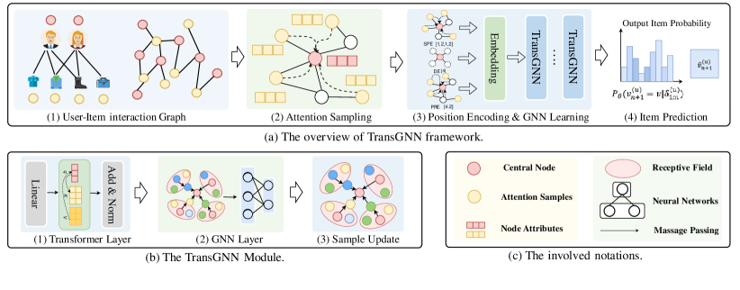
Figure 1. The framework of TransGNN. We first sample relevant nodes for the central nodes, then we calculate positional encoding to enhance the raw attributes by combining the structure information. In the TransGNN module, the Transformer layer and GNN layer improve each other, followed by the samples update sub-module.

3. Methodology

This section begins with an exposition of the TransGNN framework, followed by a detailed elucidation of each constituent component. Subsequently, we delve into a theoretical examination of TransGNN’s expressive capacity and conduct an analysis of its computational complexity.

3.1. Model Framework

The framework of TransGNN is shown in Figure 1, which consists of three important components: (1) attention sampling module, (2) positional encoding module, (3) TransGNN module. We first sample the most relevant nodes for each central node by considering the semantic similarity and graph structure information in the attention sampling module. Then in the positional encoding module, we calculate the positional encoding to help the Transformer capture the graph topology information. After these two modules, we use the TransGNN module, which contains three sub-modules in order: (i) Transformer layer, (ii) GNN layer, (iii) samples update sub-module. Among them, the Transformer layer is used to expand the receptive field of the GNN layer and aggregate the attention samples information efficiently, while the GNN layer helps the Transformer layer perceive the graph structure information and obtain more relevant information of neighbor nodes. The samples update sub-module is integrated to update the attention samples efficiently.

3.2. Attention Sampling Module

Calculating attention across the entire user-item interaction graph presents two notable challenges: (i) The computational complexity of attention calculation scales quadratically ($O(N^{2})$), which becomes impractical for large-scale recommender systems. (ii) Under the global attention setting, irrelevant user-item interactions are also incorporated, leading to suboptimal performance.

In the context of recommender systems, we posit that it is unnecessary to compute attention across the entire graph for each node. Instead, prioritizing the most relevant nodes is sufficient, thereby reducing computational complexity and eliminating noisy node information. Consequently, we advocate for sampling the most pertinent nodes for a given user or item node within the attention sampling module. To facilitate this, we commence by computing the semantic similarity matrix:

(1) $$\mathbf{S}=\mathbf{X}\mathbf{X}^{\top},$$

where $\mathbf{X}\in\mathbb{R}^{N\times d}$ consists of nodes’ attributes. However, through $\mathbf{S}$ we can only get the raw semantic similarity, overlooking the structural intricacies of user preferences. Recognizing that a user’s preference for one item might influence their affinity for another (due to shared attributes or latent factors), we refine our similarity measure by considering the neighbor nodes’ preference before sampling. We use the following equation to update the similarity matrix to incorporate the preferences of neighboring nodes:

(2) $$\mathbf{S}=\mathbf{S}+\alpha\hat{\mathbf{A}}\mathbf{S},$$

where $\alpha$ is the balance factor, and in this paper, we set $\alpha$ as 0.5. $\hat{\mathbf{A}}=\mathbf{A}+\mathbf{I}$ where $\mathbf{A}\in\mathbb{R}^{N\times N}$ is the adjacent matrix and $\mathbf{I}$ is the identity matrix. Based on the new similarity matrix $\mathbf{S}\in\mathbb{R}^{N\times N}$, for every node $v_{i}\in\mathcal{V}$ in the input graph, we sample the most relevant nodes as its attention samples as follows:

Attention samples: Given an input graph $\mathcal{G}$ and its similarity matrix $\mathbf{S}$, for node $v_{i}$ in the graph, we define its attention samples as set $\text{Smp}(v_{i})=\left\{v_{j}|v_{j}\in V\,\text{and}\,S(i,j)\in\text{top-k}(S(i,:))\right\}$ where $S(i,:)$ denotes the $i$-th row of $\mathbf{S}$ and the $k$ works as a hyper-parameter which decides how many nodes should be attended attention.

3.3. Positional Encoding Module

User-item interactions in recommender systems embody intricate structural information, critical for deriving personalized recommendations. Unlike the grid-like data where the sequential patterns can be easily captured by Transformer, interaction graphs present a more challenging topology to navigate. To enrich Transformers with this topological knowledge, we introduce three distinct positional encodings tailored for recommendation scenarios: (i) Shortest path hop based positional encoding. (ii) Degree-based positional encoding. (iii) PageRank based positional encoding. The first two encoding signify the proximity between users and items, emphasizing the diversity and frequency of user interactions or the popularity of items. Meanwhile, the last encoding indicates the significance determined by the graph topology.

3.3.1. Shortest Path Hop based Positional Encoding

User-item proximity in interaction graphs can hint at user preferences. For every user, the distance to various items (or vice versa) can have distinct implications. We encapsulate this by leveraging shortest path hops. Specifically, we denote the shortest path hop matrix as $\mathbf{P}$ and for each node $v_{i}\in\mathcal{V}$ and its attention sample node $v_{j}\in\text{Smp}(v_{i})$ the shortest path hop is $P(i,j)$, we calculate the shortest path hop based positional encoding(SPE) for every attention sample node $v_{j}$ as:

(3) $$\text{SPE}(v_{i},v_{j})=\text{MLP}(P(i,j)),$$

where $\text{MLP}(\cdot)$ is implemented as a two-layer neural network.

3.3.2. Degree based Positional Encoding

The interaction frequency of a user, or the popularity of an item, plays a pivotal role in recommendations. An item’s popularity or a user’s diverse taste can be harnessed using their node degree in the graph. Therefore, we propose to use the degree to calculate the positional encoding. Formally, for any node $v_{i}$ whose degree is $\text{deg}_{i}$, we calculate the degree based positional encoding(DE) as:

(4) $$\text{DE}(v_{i})=\text{MLP}(\text{deg}_{i}).$$

3.3.3. Page Rank based Positional Encoding

Certain users or items exert more influence due to their position in the interaction graph. PageRank offers a way to gauge this influence, facilitating better recommendations. In order to obtain the influence of structure importance, we propose to calculate positional encoding based on the page rank value for every node. Formally, for node $v_{i}$ we denote its page rank value as $\text{Pr}(v_{i})$, and we calculate the page rank based positional encoding(PRE) as:

(5) $$\text{PRE}(v_{i})=\text{MLP}(\text{Pr}(v_{i})).$$

By aggregating the above encodings with raw user/item node attributes, we enrich the Transformer’s understanding of the recommendation landscape. Specifically, for the central node $v_{i}$ and its attention samples $\text{Smp}(v_{i})$, we aggregate the positional encoding in the following ways:

(6) $$\mathbf{h}_{i}=\text{COMB}(\text{AGG}(\mathbf{x}_{i},\text{SPE}(v_{i},v_{i}),\text{DE}(v_{i}),\text{PRE}(v_{i})))$$

$$\mathbf{h}_{j}=\text{COMB}(\text{AGG}(\mathbf{x}_{j},\text{SPE}(v_{i},v_{j}),\text{DE}(v_{j}),\text{PRE}(v_{j})))\,v_{j}\in\text{Smp}(v_{i})$$

where $\mathbf{x}_{i},\mathbf{x}_{j}$ are the raw attributes of $v_{i},v_{j}$ respectively, $\text{AGG}(\cdot)$ is the aggregation function and $\text{COMB}(\cdot)$ is the combination function. In this paper, we use a two-layer MLP as $\text{COMB}(\cdot)$ and vector concatenation as $\text{AGG}(\cdot)$.

3.4. TransGNN Module

Traditional Graph Neural Networks (GNNs) exhibit limitations in comprehending the expansive relationships between users and items, due to their narrow receptive fields and the over-smoothing issue in deeper networks. Crucially, relevant items for users might be distant in the interaction space. Although Transformers can perceive long-range interactions, they often miss out on the intricacies of structured data in recommendation scenarios, further challenged by computational complexities. The TransGNN module synergizes the strengths of GNNs and Transformers to alleviate these issues. This module consists of: (i) Transformer layer, (ii) GNN layer, and (iii) samples update sub-module.

3.4.1. Transformer Layer

To optimize user-item recommendation, the Transformer layer broadens GNN’s horizon, focusing on potentially important yet distant items. In order to lower the complexity and filter out the irrelevant information, we only consider the most relevant samples for each central node. In the following, we use central node $v_{i}$ and its attention samples $\text{Smp}(v_{i})$ as an example to illustrate the Transformer layer, and for other nodes, this process is the same.

We denote the input of Transformer layer as $\mathbf{H}\in\mathbb{R}^{N\times d_{\text{in}}}$ and the representation of central node $v_{i}$ is $h_{i}$. We stack the representations of attention samples $\text{Smp}(v_{i})$ as the matrix $\mathbf{H}^{\text{Smp}}_{i}\in\mathbb{R}^{k\times d_{\text{in}}}$. We use three matrices $\mathbf{W}_{q},\mathbf{W}_{k},\mathbf{W}_{v}\in\mathbb{R}^{d_{\text{in}}\times d_{\text{out}}}$ to project the corresponding representations to $\mathbf{Q}$, $\mathbf{K}$ and $\mathbf{V}$ respectively and we aggregate the information based on the attention distribution as:

(7) $$\mathbf{h}_{i} =\text{softmax}(\frac{\mathbf{Q}\mathbf{K}^{\top}}{\sqrt{d_{\text{out}}}})V$$

where

(8) $$\begin{cases}\mathbf{Q}&=\mathbf{h}_{i}\mathbf{W}_{Q},\\ \mathbf{K}&=\mathbf{H}^{\text{Smp}}_{i}\mathbf{W}_{k},\\ \mathbf{V}&=\mathbf{H}^{\text{Smp}}_{i}\mathbf{W}_{v}\\ \end{cases}$$

in which $\mathbf{Q}$ is the representation of the query and $\mathbf{K},\mathbf{V}$ are the representation of keys and values. This process can be expanded to multi-head attention as:

(9) $$\text{MultiHead}(\mathbf{h}_{i})=\text{Concat}(\text{head}_{1},...,\text{head}_{m})\mathbf{W}_{m},$$

where $m$ is the head number, $\text{Concat}(\cdot)$ denotes the concatanate function and $\mathbf{W}_{m}$ is the projection matrix, each head is calculated as $\mathbf{h}_{i}$ in Equation 7.

3.4.2. GNN Layer

Incorporating interactions and structural nuances, this layer aids the Transformer in harnessing the user-item interaction graphs more profoundly. Given node $v_{i}$, the message passing process of the GNN layer can be described as:

(10) $$\mathbf{h}_{M}(v_{i})=\text{Message}(\mathbf{h}_{k},\forall v_{k}\in\mathcal{N}(v_{i}))$$

$$\mathbf{h}_{i}=\text{Combine}(\mathbf{h}_{i},\mathbf{h}_{M}(v_{i})),$$

where $\mathcal{N}(v_{i})$ is the neighbor nodes set of $v_{i}$. $h_{i},h_{k}$ are the representations of $v_{i},v_{k}$ respectively. $\text{Message}(\cdot)$ and $\text{Combine}(\cdot)$ are the message passing function and aggregation function defined by GNN layer.

3.4.3. Samples Update Sub-Module

After the Transformer and GNN layers, the attention samples should be updated upon new representations. However, directly calculating the similarity matrix incurs a computational complexity of $O(N^{2})$. Here we introduce two efficient strategies for updating the attention samples.

(i) Random Walk based Update

Recognizing the tendency of users to exhibit consistent taste profiles, this approach delves into the local neighborhoods of each sampled item to uncover potentially relevant items. We employ a random walk strategy to explore the local neighborhood of every sampled node. Specifically, the transition probability of the random walk is determined based on the similarity, as follows:

(11) $$p_{i\to j}=\begin{cases}\frac{\mathbf{h}_{i}\mathbf{h}_{j}^{T}}{\sum_{l\in\mathcal{N}(v_{i})}\mathbf{h}_{i}\mathbf{h}_{l}^{\top}},&\text{if $v_{j}\in\mathcal{N}(v_{i})$}\\ 0,&\text{if $v_{j}\not\in\mathcal{N}(v_{i})$}\end{cases}$$

The transfer probability can be calculated efficiently in the message passing process. Based on the transfer probability, we walk a node sequence with length $L$ for each attention sample, and then we choose the new attention samples among the explored nodes upon new representations.

(ii) Message Passing based Update

The random walk-based update strategy has extra overhead. We propose another update strategy that utilizes the message passing of the GNN layer to update the samples without extra overhead. Specifically, we aggregate the attention samples from the neighbor nodes for each central node in the message passing process of the GNN layer. The intuition behind this is that the attention samples of the neighbors may also be the relevant attention samples of the central nodes. We denote the attention samples set of the neighbor nodes as the attention message, which is defined as follows:

(12) $$\text{Attn\_Msg}(v_{i})=\bigcup\text{Smp}(v_{j})\;\forall v_{j}\in\mathcal{N}(v_{i}),$$

thus we choose the new attention samples among $\text{Attn\_Msg}(v_{i})$ for node $v_{i}$ based on the new representations.

3.5. Model Optimization

For training our TransGNN model, we employ the pairwise rank loss to optimize the relative ranking of items (Chen et al., 2009):

(13) $$\mathcal{L}=\Sigma_{\mathcal{u}\in\mathcal{U}}\Sigma_{t=1}^{n}\log(\sigma(P(i_{t+1})-P(i_{t+1}^{-}))),$$

where we pair each ground-truth item $i_{t+1}$ with a negative item $i_{t+1}^{-}$ that is randomly sampled. $P(i_{t+1})$ and $P(i_{t+1}^{-})$ are prediction scores given by TransGNN, $\sigma(.)$ denotes the sigmoid function.

3.6. Complexity Analysis

Here the complexity of TransGNN is presented and discussed. The overhead of the attention sampling module and the positional encoding module can be attributed to the data pre-processing stage. The complexity of the attention sampling module is $O(N^{2})$, and the most complex part of the positional encoding module is the calculation of the shortest hop matrix $\mathbf{P}$. Considering the graphs in real applications are sparse and have positive edge weights, Johnson algorithm (Allaoui and Artiba, 2009) can be employed to facilitate the analysis. With the help of the heap optimization, the time and space complexity can be reduced to $O(N(N+E)\log E)$ where $N$ is the node number, and $E$ is the edge number. The extra overhead of the TransGNN module compared with GNNs mainly focus on the Transformer layer and attention samples update. The extra complexity caused by the Transformer layer is $O(Nk)$ where $k$ is the attention samples number, and the extra complexity of samples update is $O(Nkd_{a})$ for message passing mechanism where $d_{a}$ is the average degree (the extra complexity will be $O(NkL)$ if we use random walk-based update). Therefore, we show that TransGNN has at most $O(N(N+E)\log E)$ data pre-processing complexity and linear extra complexity compared with GNNs because $kd_{a}$ is a constant and $kd_{a}<<N$.

3.7. Theoretical Analysis

Here we demonstrate the expression power of TransGNN via following two theorems with their proofs.

Theorem 1.

TransGNN has at least the expression ability of GNN, and any GNN can be expressed by TransGNN.

Proof.

If we add attention mask as top $1$ mask, the Eqn of Transformer layer will become:

(14) $$\mathbf{H}_{\text{out}}=\frac{1}{\sqrt{d_{\text{out}}}}\mathbf{H}(\mathbf{W}_{v}+\mathbf{I})$$

We use the GCN layer as an example and the message passing can be derived as:

(15) $$\mathbf{H} =\sigma(\mathbf{A}\mathbf{H}_{\text{out}}\mathbf{W})$$

$$=\sigma(\mathbf{A}\frac{1}{\sqrt{d_{\text{out}}}}\mathbf{H}(\mathbf{W}_{v}+\mathbf{I})\mathbf{W}),$$

where $\sigma(\cdot)$ is the activation function and if we set $\mathbf{W}_{v}$ as diagonal matrix with the diagonal value as $\sqrt{d_{\text{out}}}-1$ and the Equation 15 will become:

(16) $$\mathbf{H}=\sigma(\mathbf{A}\mathbf{H}\mathbf{W})$$

Therefore, TransGNN has at least the expression ability of GNN. ∎

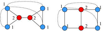
Figure 2. Example illustration. The dotted line denotes the receptive field of the Transformer layer, and the color denotes the similarity relationship.

Theorem 2.

TransGNN can be more expressive than 1-WL Test.

Proof.

With the help of Transformer layer and positional encoding, TransGNN can aggregate more relevant information and structure information to improve the message passing process, which can be more expressive than 1-WL Test (Douglas, 2011). We give an illustration in Figure 2. These two graphs cannot be distinguished by 1-WL Test. However, because the transformer layer expand the receptive field and the positional encoding can capture the local structure, they can be distinguish by TransGNN. For example the node in the top left gets the shortest path information {0,1,3,3} and {0,1,2,3} respectively. ∎

4. Experiments

To evaluate the effectiveness of our TransGNN, our experiments are designed to answer the following research questions:

• RQ1: Can our proposed TransGNN outperform the state-of the-art baselines of different categories?

• RQ2: How do the key components of TransGNN (e.g., the attention sampling, postional encoding, the message passing update) contribute to the overall performance on different datasets?

• RQ3: How do different hyper-parameters affect TransGNN?

• RQ4: How does TransGNN perform under different GNN layers?

• RQ5: How efficient is TransGNN compared to the baselines?

• RQ6: How does the visualization of representations of TransGNN compared to the baselines?

4.1. Experimental Settings

4.1.1. Datasets.

We evaluate the proposed model on five real-world representative datasets (i.e., Yelp, Gowalla, Tmall, Amazon-Book, and MovieLens), which vary significantly in domains and sparsity:

• Yelp: This commonly-used dataset contains user ratings on business venues collected from Yelp. Following other papers on implicit feedback (Huang et al., 2021), we treat users’ rated venues as interacted items and treat unrated venues as non-interacted items.

• Gowalla: It contains users’ check-in records on geographical locations obtained from Gowalla. This evaluation dataset is generated from the period between 2016 and 2019.

• Tmall: This E-commerce dataset is released by Tmall, containing users’ behaviors for online shopping. We collect the page-view interactions during December in 2017.

• Amazon-Book: Amazon-review is a widely used dataset for product recommendation (He and McAuley, 2016). We select Amazon-book from the collection. Similarly, we use the 10-core setting to ensure that each user and item have at least ten interactions.

• MovieLens: This is a popular benchmark dataset for evaluating recommendation algorithms (Harper and Konstan, 2015). In this work, we adopt the well-established version, MovieLens 10m (ML-10m), which contains about 10 million ratings of 10681 movies by 71567 users. The users of MovieLens 10M dataset are randomly chosen and each user rated at least 20 movies.

For dataset preprocessing, we follow the common practice in (Huang et al., 2021; Xia et al., 2022; Tang and Wang, 2018). For all datasets, we convert all numeric ratings or the presence of a review to implicit feedback of 1 (i.e., the user interacted with the item). After that, we group the interaction records by users and build the interaction sequence for each user by sorting these interaction records according to the timestamps. To ensure the quality of the dataset, following the common practice (Huang et al., 2021; Xia et al., 2022; Tang and Wang, 2018; Sun et al., 2019), we filtered out users and items with too few interactions. The statistics of the datasets are summarized in Table 1.

4.1.2. Evaluation Protocols.

Following the recent CF models (He et al., 2020; Wu et al., 2021), we adopt all-rank evaluation protocol. Under this protocol, during the evaluation of a user, both the positive items from the test set and all the non-interacted items are collectively ranked and assessed. For the assessment of recommendation performance, we have opted for widely recognized metrics, namely, Recall@N and Normalized Discounted Cumulative Gain (NDCG@N) (Ren et al., 2020; Wang et al., 2019a). The value of N in these metrics is set to 20 and 40.

Table 1. Statistics of datasets after preprocessing

Datasets	# Users	# Items	# Interactions	Density
Yelp	29,601	24,734	1,527,326	$2.1\times 10^{-3}$
Gowalla	50,821	24,734	1,069,128	$4.0\times 10^{-4}$
Tmall	47,939	41,390	2,357,450	$1.2\times 10^{-3}$
Amazon-Book	78,578	77,801	3,200,224	$5.2\times 10^{-4}$
ML-10M	69,878	10,196	9,998,816	$1.4\times 10^{-2}$

Table 2. Comparison of recommendation performance with baseline models in numerical values. The results of the best performing baseline are underlined. The numbers in bold indicate statistically significant improvement (p ¡ .01) by the pairwise t-test comparisons over the other baselines. ^⋆, ^∗, ^† and ^‡ denote GNN-based, HGNN-based, SSL-enhanced and Transformer-GNN-based models, respectively.

Dataset	Metric	(a)	(b)	(c)	(d)	(e)	(f)	(g)	(h)	(i)	(j)	(k)	(l)	(m)	(n)
		AutoR	GCMC⋆	PinSage⋆	NGCF⋆	LightGCN⋆	GCCF⋆	HyRec∗	DHCF∗	MHCN†	SLRec†	SGL†	SHT‡	TransGNN	Improv.
Yelp	Recall@20	0.0348	0.0462	0.0471	0.0579	0.0653	0.0462	0.0467	0.0458	0.0646	0.0639	0.0675	0.0651	0.0817	+21.04%
	Recall@40	0.0515	0.0836	0.0895	0.1131	0.1203	0.0930	0.0891	0.0851	0.1226	0.1221	0.1269	0.1091	0.1506	+18.68%
	NDCG@20	0.0236	0.0379	0.0393	0.0477	0.0532	0.0398	0.0355	0.0376	0.0410	0.0358	0.0555	0.0546	0.0734	+32.25%
	NDCG@40	0.0358	0.0443	0.0417	0.0693	0.0828	0.0704	0.0628	0.0716	0.0810	0.0806	0.0871	0.0709	0.0999	+14.70%
Tmall	Recall@20	0.0235	0.0292	0.0373	0.0402	0.0525	0.0327	0.0333	0.0385	0.0405	0.0394	0.0436	0.0387	0.0608	+15.81%
	Recall@40	0.0405	0.0511	0.0594	0.0613	0.0867	0.0619	0.0677	0.0784	0.0783	0.0782	0.0802	0.0645	0.0989	+14.07%
	NDCG@20	0.0120	0.0147	0.0221	0.0294	0.0372	0.0257	0.0262	0.0318	0.0337	0.0354	0.0363	0.0262	0.0422	+13.44%
	NDCG@40	0.0103	0.0200	0.0310	0.0405	0.0508	0.0402	0.0428	0.0417	0.0473	0.0413	0.0505	0.0352	0.0555	+9.25%
Gowalla	Recall@20	0.1298	0.1395	0.1380	0.1570	0.1820	0.1577	0.1649	0.1642	0.1710	0.1656	0.1709	0.1232	0.1887	+3.68%
	Recall@40	0.1359	0.1783	0.1852	0.2270	0.2531	0.2348	0.2333	0.2422	0.2347	0.2331	0.2502	0.1804	0.2640	+4.31%
	NDCG@20	0.1178	0.1204	0.1196	0.1327	0.1547	0.1285	0.1452	0.1453	0.1510	0.1473	0.1529	0.0731	0.1602	+3.56%
	NDCG@40	0.0963	0.1060	0.1035	0.1102	0.1270	0.1150	0.1162	0.1256	0.1230	0.1213	0.1259	0.0881	0.1318	+3.78%
Amazon-Book	Recall@20	0.0287	0.0288	0.0282	0.0344	0.0411	0.0415	0.0427	0.0411	0.0552	0.0521	0.0478	0.0740	0.0801	+8.24%
	Recall@40	0.0492	0.0539	0.0625	0.0590	0.0741	0.0772	0.0793	0.0824	0.0846	0.0815	0.1023	0.1164	0.1239	+6.44%
	NDCG@20	0.0156	0.0224	0.0219	0.0263	0.0318	0.0308	0.0330	0.0312	0.0384	0.0356	0.0379	0.0553	0.0603	+9.04%
	NDCG@40	0.0228	0.0336	0.0392	0.0364	0.0461	0.0440	0.0432	0.0414	0.0492	0.0475	0.0531	0.0690	0.0748	+8.41%
ML-10M	Recall@20	0.1932	0.2015	0.2251	0.2136	0.2402	0.2356	0.2371	0.2368	0.2509	0.2415	0.2474	0.2546	0.2668	+4.79%
	Recall@40	0.2593	0.2726	0.3050	0.3127	0.3406	0.3321	0.3376	0.3263	0.3424	0.3380	0.3603	0.3794	0.3962	+4.43%
	NDCG@20	0.1903	0.2052	0.2359	0.2218	0.2704	0.2682	0.2691	0.2697	0.2761	0.2725	0.2813	0.3038	0.3223	+6.09%
	NDCG@40	0.2180	0.2349	0.2452	0.2421	0.2874	0.2802	0.2814	0.2846	0.3007	0.2932	0.3194	0.3384	0.3525	+4.17%

4.1.3. Baselines.

We compare TransGNN with five types of baselines: (1) Autoencoder-based method, i.e., AutoR (Sedhain et al., 2015). (2) GNN-based methods, which includes GCMC (Berg et al., 2017), PinSage (Ying et al., 2018), NGCF (Wang et al., 2019a), LightGCN (He et al., 2020) and GCCF (Chen et al., 2020). (3) Hypergraph-based methods, which includes HyRec (Wang et al., 2020) and DHCF (Ji et al., 2020). (4) Self-supervised learning enhanced GNN-based methods, which includes MHCN (Yu et al., 2021), SLRec (Yao et al., 2021) and SGL (Wu et al., 2021). (5) To verify the effectiveness of our integration of Transformer and GNNs, we also include the Hypergraph Transformer and Self-supervised learning enhanced method, i.e., SHT (Xia et al., 2022) in comparison.

4.1.4. Reproducibility.

We use three Transformer layers with two GNN layers sandwiched between them. For the transformer layer, multi-head attention is used. For the GNN layer, we use GraphSAGE as the backbone model. We adopt the message passing based attention update in our main experiment. We consider attention sampling size $d\in\{5,10,15,20,25,30,35\}$ , number of heads $h\in\{2,4,8,16,32\}$, dropout ratio $d\in[0,1]$ and weight decay $d\in[0,1e^{-2}]$. We apply grid search to find the optimal hyper-parameters for each model. We use Adam to optimize our model. We train each model with early stop strategies until the validation recall value does not improve for 20 epochs on a single NVIDIA A100 SXM4 80GB GPU. The average results of five runs are reported.

4.2. Overall Performance Comparison (RQ1)

In this section, we validate the effectiveness of our TransGNN framework by conducting the overall performance evaluation on the five datasets and comparing TransGNN with various baselines. The results are presented in Table 2.

Compared with Autoencoder-based methods like AutoR, we observe that GNN-based methods, including TransGNN, exhibit superior performance. This can be largely attributed to the inherent ability of GNNs to adeptly navigate and interpret the complexities of graph-structured data. Autoencoders, while efficient in latent feature extraction, often fall short in capturing the relational dynamics inherent in user-item interactions, a forte of GNNs. When considering hypergraph neural networks (HGNNs) such as HyRec and DHCF, it’s apparent that they surpass many GNN-based methods (e.g., GCMC, PinSage, NGCF, STGCN). The key to this enhanced performance lies in their ability to capture high-order and global graph connectivity, a dimension where conventional GNNs often exhibit limitations. This observation underscores the necessity of models that can comprehend more intricate and interconnected graph structures in recommendation systems. TransGNN stands out by integrating the Transformer’s strengths, particularly in expanding the receptive field. This integration enables TransGNN to focus on a broader and more relevant set of nodes, thereby unlocking the latent potential of GNNs in global relationship learning. This synthesis is particularly effective in capturing long-range dependencies, which is a notable limitation in standalone GNNs.

In the realm of Self-Supervised Learning (SSL), methods like MHCN, SLRec, and SGL have shown improvements in graph-based Collaborative Filtering models. These advancements are primarily due to the incorporation of augmented learning tasks which introduce beneficial regularization to the parameter learning processes. This strategy effectively mitigates overfitting risks based on the input data itself. However, TransGNN surpasses these SSL baselines, a success we attribute to its global receptive field facilitated by the Transformer architecture. This global perspective enables the adaptive aggregation of information at a larger scale, in contrast to SSL-based methods which are constrained to batch-level sampling, limiting their scope. Moreover, SSL methods often lack the robustness required to effectively tackle data noise. TransGNN, with its attention sampling module, adeptly addresses this challenge by filtering out irrelevant nodes, thereby refining the graph structure and significantly reducing noise influence.

An intriguing aspect of TransGNN’s performance is observed under different top-K settings in evaluation metrics like Recall@K and NDCG@K. Notably, TransGNN demonstrates more substantial performance improvements over baseline models when K is smaller. This is particularly relevant considering the position bias in recommendation systems, where users are more inclined to focus on higher-positioned items in recommendation lists. TransGNN’s efficacy in these scenarios suggests it is well-suited for generating user-friendly recommendations that align closely with user preferences, especially at the top of the recommendation list.

Table 3. Ablation studies on different components.

Category	Data	Yelp		Gowalla		Tmall
	Variants	Recall	NDCG	Recall	NDCG	Recall	NDCG
Attention Sampling	-AS	0.0686	0.0583	0.1492	0.0961	0.0418	0.0349
Positional Encoding	-SPE	0.0910	0.0760	0.1836	0.1104	0.0591	0.0412
	-DE	0.0922	0.0781	0.1873	0.1109	0.0602	0.0416
	-PRE	0.0907	0.0772	0.1845	0.1106	0.0595	0.0417
	-PE	0.0704	0.0610	0.1609	0.1013	0.0437	0.0375
TransGNN	-Trans	0.0479	0.0391	0.0978	0.0556	0.0237	0.0159
	-GNN	0.0390	0.0316	0.0574	0.0341	0.0209	0.0126
Attention Update	+RW	0.0924	0.0782	0.1880	0.1109	0.0601	0.0417
	-MP	0.0723	0.0611	0.1550	0.1007	0.0462	0.0360
Original	TransGNN	0.0927	0.0787	0.1887	0.1121	0.0608	0.0422

4.3. Ablation Study (RQ2)

To validate the effectiveness of the proposed modules, we individually remove the applied techniques in the four major parts of TransGNN, i.e., the attention sampling module (-AS), the positional encoding module (-PE), the TransGNN module (-Trans and -GNN) and the attention update module (-MP). We also ablate the detail components in our positional encoding module and attention update module. Specifically, we remove the shortest-path-hop-based (-SPE), degree-based (-DE) and pagerank-based (-PRE) positional encoding, respectively. For the attention update module, we also substitute the message passing based attention update into random walk-based update (+RW). We use GraphSAGE as the backbone GNN to report the performance when ignoring different components. All the settings are the same as the default. The variants are re-trained for test on Yelp, Gowalla and Tmall datasets. From Table 3, we have the following major conclusions:

• When the attention sampling module is removed (-AS), a noticeable performance drop is observed across all datasets. This highlights the critical role of the attention sampling strategy in TransGNN, which effectively filters out irrelevant nodes in a global attention context. Without this module, the model becomes less discerning in its node selection, leading to less targeted and potentially less relevant recommendations. This underlines the importance of focused attention in managing the vast and complex user-item interaction space.

• The exclusion of the positional encoding module (-PE) leads to compromised results, indicating that the Transformer layer alone cannot capture the structure information adequately. This is further substantiated by the reduced performance observed when individual components of the positional encoding—shortest-path-hop-based (-SPE), degree-based (-DE), and PageRank-based (-PRE)—are separately removed. Each of these encodings contributes uniquely to the model’s understanding of the graph topology, reflecting user-item proximity, interaction frequency, and structural importance, respectively.

• The simultaneous necessity of both the Transformer and GNN layers is clearly demonstrated when either is removed (-Trans and -GNN). The significant decline in performance underscores the synergistic relationship between these two layers. The Transformer layer, with its expansive receptive field, brings a global perspective to the table, while the GNN layer contributes a comprehensive understanding of graph topology. Their combined operation is crucial for a holistic approach to user modeling in TransGNN, blending global and local insights.

• In examining the sampling update strategies, it is observed that the random walk-based update (+RW) does not perform as well as the message passing-based update. This could be attributed to the inherent noise in the edges, which might lead the random walk to less relevant nodes, highlighting the superiority of a more structured update mechanism.

• Finally, the absence of the message passing update strategy (-MP) results in a performance decline. This suggests that static attention samples might become outdated or incomplete as the model iterates through training. The dynamic nature of the message passing update ensures that the attention samples remain relevant and reflective of the evolving user-item interactions. This dynamic updating is crucial in maintaining the accuracy and relevance of the recommendations, as it allows TransGNN to adapt to changes in user preferences and item attributes.

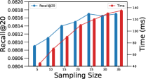
(a) Sampling size influence.

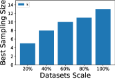
(b) Best size of different data scale.

Figure 3. Different sampling size influence and best sampling size for different graph scale.

4.4. Attention Sampling Study (RQ3)

We study the influence of attention sampling size using Yelp as an example. The results can be found in Figure 3. We have the following observations:

• In Figure 3(a), when $k$ is varied from 5 to 35, a clear pattern emerges. Sampling fewer nodes, while computationally less demanding, leads to a noticeable compromise in performance. This can be attributed to the fact that with too few nodes sampled, the model might miss out on critical information necessary for accurate recommendations. Essential connections in the user-item graph could be overlooked, leading to a less robust understanding of user preferences and item characteristics. On the other end of the spectrum, sampling an excessive number of nodes does not yield proportional improvements in performance. This plateau in performance gain despite increased sampling can be linked to the model encountering a saturation point. Beyond a certain threshold, additional nodes do not contribute new or relevant information; instead, they add to the computational burden without enhancing the model’s ability to make accurate predictions.

• In Figure 3(b) we change the graph scale and show the best sampling size. Interestingly, we find that a relatively small sampling size is found to be sufficient for achieving good performance. This finding is significant as it suggests that TransGNN can operate efficiently without necessitating extensive computational resources. The ability to extract meaningful insights from a smaller subset of nodes underscores the effectiveness in identifying the most pertinent information from the user-item interaction graph.

• Furthermore, when the scale of the graph is varied, it is observed that only a marginal increase in the number of samples is required as the graph size expands. This is a particularly important observation as it indicates the scalability of TransGNN. Even as the complexity of the graph increases, the model does not require a proportionately large increase in resources to maintain its performance. This scalability is crucial for practical applications where the size of the dataset can be large and varied.

Table 4. Performance comparison between SHT and TransGNN at different layers.

Layer #	Method	Amazon-Book
		Recall@20	NDCG@20
1 Layer	SHT	0.0712	0.0497
	TransGNN	0.0723	0.0502
2 Layer	SHT	0.0740	0.0553
	TransGNN	0.0772	0.0565
3 Layer	SHT	0.0725	0.0541
	TransGNN	0.0801	0.0603
4 Layer	SHT	0.0713	0.0513
	TransGNN	0.0805	0.0606
5 Layer	SHT	0.0684	0.0467
	TransGNN	0.0807	0.0609

4.5. Study on the number of GNN Layers (RQ4)

Our investigation focuses on evaluating the performance implications stemming from alterations in the number of GNN layers, as outlined in Table 4. Within this analysis, the performance of SHT exhibits improvement up to a two-layer configuration but exhibits degradation with the inclusion of additional layers, suggesting the onset of over-smoothing phenomena within deeper network architectures. In contrast, TransGNN displays augmented performance metrics with an escalating count of layers, indicative of its efficacy in mitigating over-smoothing effects and capturing extensive dependencies across the graph structure. This observed disparity underscores TransGNN’s advanced adeptness in navigating the complexities inherent in deeper graph networks, thereby establishing it as a robust solution for recommendation systems.

4.6. Complexity and Efficiency Analysis (RQ5)

We conduct an analysis on TransGNN’s execution efficacy, as delineated in Table 5. Comparing with GNN-based (i.e., NGCF), Hypergraph-based (i.e., HyRec) and Transformer-GNN-based baselines (i.e., SHT), we have the following observations:

• TransGNN has a relatively fewer GPU memory cost. This efficiency stems from the model’s node sampling strategy for the Transformer component, which circumvents the need for attention calculations across the entire graph. By targeting only the most relevant nodes, TransGNN significantly cuts down on the computational load that would typically be associated with processing large graphs. This approach not only conserves memory but also makes the model more agile and adaptable to varying dataset sizes and complexities.

• TransGNN has better efficiency in both training ($30\%~{}40\%$ less time) and inference ($30\%-40\%$ less time) compared with NGCF. The time saved in both training and inference phases makes TransGNN a viable option for scenarios where speed is of the essence, such as real-time recommendation systems or applications with frequent model updates.

• Furthermore, TransGNN achieves comparable, if not superior, training and inference times relative to DHCF and SHT, while simultaneously maintaining a smaller memory footprint. This balance between speed and resource utilization is crucial in scenarios where computational resources are limited. The lower memory requirement, quantified at $20\%~{}30\%$ less than the other models, underscores TransGNN’s suitability for deployment in environments with constrained computational resources.

• Additionally, TransGNN’s minimal Floating Point Operations (FLOPs) compared to all baselines is a testament to its computational efficiency. This aspect is particularly important for deployment on low-resource devices, where managing computational overhead is critical. The lower FLOPs indicate that TransGNN requires fewer computational resources to perform the same tasks as its counterparts, which is a significant advantage in resource-constrained environments.

Table 5. Parameters number and execution efficiency analysis of models on Yelp dataset.

Yelp	TransGNN	NGCF	HyRec	SHT
# Parameters	1.77M	2.30M	1.91M	1.75M
# GPU Memory	1.79GB	0.62GB	2.32GB	2.33GB
# FLOPs ($\times 10^{6}$)	3.74	8.41	5.36	4.89
Training Cost (per epoch)	4.75s	7.88s	3.65s	3.97s
Inference Cost (per epoch)	16.95s	27.07s	12.48s	12.57s
Recall@20	0.0927	0.0294	0.0472	0.0651

4.7. Visualization (RQ6)

We visualize the user interaction sequence embedding for different candidate next-click items by t-SNE (Van der Maaten and Hinton, 2008). We conduct the visualization on Yelp with eight different target items, and each target item has more than 1000 query sequence pairs. The results are shown in Figure 4. From the results, we can find that the cluster property of the representations produced by GNNs-based baselines is not as good as that of ours. This difference can be attributed to certain inherent limitations of GNNs. Primarily, GNNs tend to rely heavily on edges within the graph. While this is generally effective, it can also be a drawback, particularly when the graph contains noisy or irrelevant edges. Such edges can inadvertently introduce less relevant information into the node embeddings, leading to less distinct clusters in the visualization. Besides, we also find that compared with the SHT, TransGNN can cluster the relevant nodes better, because TransGNN leverages both Transformer and GNN layers, allowing it to extend its receptive field beyond immediate neighbors. This expanded field enables TransGNN to capture a broader context, encompassing both local and more distant, yet relevant, interactions.

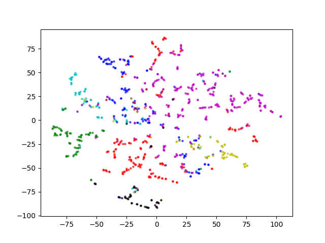
(a) Visualization of NGCF.

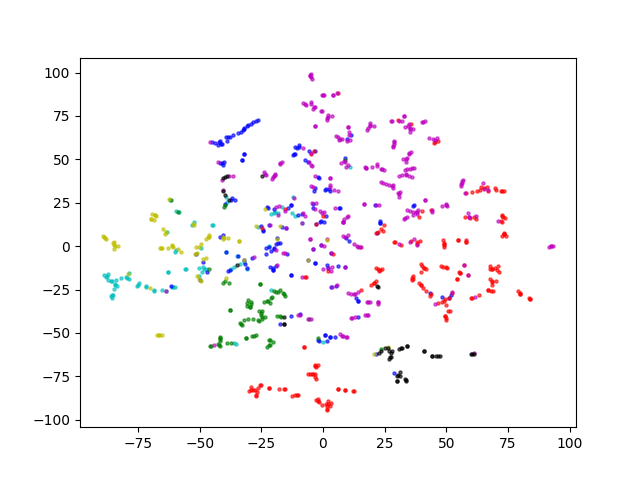
(b) Visualization of HyRec.

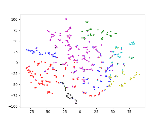
(c) Visualization of SHT.

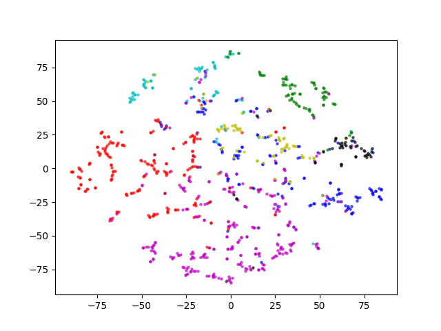
(d) Visualization of TransGNN.

Figure 4. Visualization of different baselines.

5. Conclusion

In this paper, we propose TransGNN to help GNN expand its receptive field with low overhead. We first use three kinds of positional encoding to capture the structure information for the transformer layer. Then the Transformer layer and GNN layer are used alternately to make every node focus on the most relevant samples. Two efficient sample update strategies are proposed for medium- and large-scale graphs. Experiments on five datasets show the effectiveness of TransGNN compared to the state-of-the-art baselines.

References

- (1)
- Allaoui and Artiba (2009) Hamid Allaoui and AbdelHakim Artiba. 2009. Johnson’s algorithm: A key to solve optimally or approximately flow shop scheduling problems with unavailability periods. International Journal of Production Economics 121, 1 (2009), 81–87.
- Alon and Yahav (2021) Uri Alon and Eran Yahav. 2021. On the Bottleneck of Graph Neural Networks and its Practical Implications. In 9th International Conference on Learning Representations, ICLR 2021, Virtual Event, Austria, May 3-7, 2021. OpenReview.net. https://openreview.net/forum?id=i80OPhOCVH2
- Balcilar et al. (2021) Muhammet Balcilar, Pierre Héroux, Benoit Gaüzère, Pascal Vasseur, Sébastien Adam, and Paul Honeine. 2021. Breaking the Limits of Message Passing Graph Neural Networks. In Proceedings of the 38th International Conference on Machine Learning, ICML 2021, 18-24 July 2021, Virtual Event (Proceedings of Machine Learning Research, Vol. 139), Marina Meila and Tong Zhang (Eds.). PMLR, 599–608. http://proceedings.mlr.press/v139/balcilar21a.html
- Berg et al. (2017) Rianne van den Berg, Thomas N Kipf, and Max Welling. 2017. Graph convolutional matrix completion. arXiv preprint arXiv:1706.02263 (2017).
- Cai and Wang (2020) Chen Cai and Yusu Wang. 2020. A Note on Over-Smoothing for Graph Neural Networks. CoRR abs/2006.13318 (2020). arXiv:2006.13318 https://arxiv.org/abs/2006.13318
- Chen et al. (2023) Jiawei Chen, Hande Dong, Xiang Wang, Fuli Feng, Meng Wang, and Xiangnan He. 2023. Bias and debias in recommender system: A survey and future directions. ACM Transactions on Information Systems 41, 3 (2023), 1–39.
- Chen et al. (2020) Lei Chen, Le Wu, Richang Hong, Kun Zhang, and Meng Wang. 2020. Revisiting graph based collaborative filtering: A linear residual graph convolutional network approach. In Proceedings of the AAAI conference on artificial intelligence, Vol. 34. 27–34.
- Chen et al. (2009) Wei Chen, Tie-Yan Liu, Yanyan Lan, Zhi-Ming Ma, and Hang Li. 2009. Ranking measures and loss functions in learning to rank. Advances in Neural Information Processing Systems 22 (2009).
- Chien et al. (2021) Eli Chien, Jianhao Peng, Pan Li, and Olgica Milenkovic. 2021. Adaptive Universal Generalized PageRank Graph Neural Network. In 9th International Conference on Learning Representations, ICLR 2021, Virtual Event, Austria, May 3-7, 2021. OpenReview.net.
- Collins et al. (2018) Andrew Collins, Dominika Tkaczyk, Akiko Aizawa, and Joeran Beel. 2018. A study of position bias in digital library recommender systems. arXiv preprint arXiv:1802.06565 (2018).
- Douglas (2011) Brendan L Douglas. 2011. The weisfeiler-lehman method and graph isomorphism testing. arXiv preprint arXiv:1101.5211 (2011).
- Dwivedi and Bresson (2020) Vijay Prakash Dwivedi and Xavier Bresson. 2020. A generalization of transformer networks to graphs. arXiv preprint arXiv:2012.09699 (2020).
- Fan et al. (2021) Ziwei Fan, Zhiwei Liu, Jiawei Zhang, Yun Xiong, Lei Zheng, and Philip S Yu. 2021. Continuous-time sequential recommendation with temporal graph collaborative transformer. In Proceedings of the 30th ACM international conference on information & knowledge management. 433–442.
- Guo et al. (2022) Jiayan Guo, Peiyan Zhang, Chaozhuo Li, Xing Xie, Yan Zhang, and Sunghun Kim. 2022. Evolutionary Preference Learning via Graph Nested GRU ODE for Session-based Recommendation. In Proceedings of the 31st ACM International Conference on Information & Knowledge Management. 624–634.
- Harper and Konstan (2015) F Maxwell Harper and Joseph A Konstan. 2015. The movielens datasets: History and context. Acm transactions on interactive intelligent systems (tiis) 5, 4 (2015), 1–19.
- He and McAuley (2016) Ruining He and Julian McAuley. 2016. Ups and downs: Modeling the visual evolution of fashion trends with one-class collaborative filtering. In proceedings of the 25th international conference on world wide web. 507–517.
- He et al. (2020) Xiangnan He, Kuan Deng, Xiang Wang, Yan Li, Yongdong Zhang, and Meng Wang. 2020. Lightgcn: Simplifying and powering graph convolution network for recommendation. In Proceedings of the 43rd International ACM SIGIR conference on research and development in Information Retrieval. 639–648.
- He et al. (2017) Xiangnan He, Lizi Liao, Hanwang Zhang, Liqiang Nie, Xia Hu, and Tat-Seng Chua. 2017. Neural collaborative filtering. In Proceedings of the 26th international conference on world wide web. 173–182.
- Huang et al. (2021) Chao Huang, Huance Xu, Yong Xu, Peng Dai, Lianghao Xia, Mengyin Lu, Liefeng Bo, Hao Xing, Xiaoping Lai, and Yanfang Ye. 2021. Knowledge-aware coupled graph neural network for social recommendation. In Proceedings of the AAAI conference on artificial intelligence, Vol. 35. 4115–4122.
- Ji et al. (2020) Shuyi Ji, Yifan Feng, Rongrong Ji, Xibin Zhao, Wanwan Tang, and Yue Gao. 2020. Dual channel hypergraph collaborative filtering. In Proceedings of the 26th ACM SIGKDD international conference on knowledge discovery & data mining. 2020–2029.
- Jiang et al. (2022) Juyong Jiang, Jae Boum Kim, Yingtao Luo, Kai Zhang, and Sunghun Kim. 2022. AdaMCT: adaptive mixture of CNN-transformer for sequential recommendation. arXiv preprint arXiv:2205.08776 (2022).
- Joachims et al. (2017) Thorsten Joachims, Laura Granka, Bing Pan, Helene Hembrooke, and Geri Gay. 2017. Accurately interpreting clickthrough data as implicit feedback. In Acm Sigir Forum, Vol. 51. Acm New York, NY, USA, 4–11.
- Joachims et al. (2007) Thorsten Joachims, Laura Granka, Bing Pan, Helene Hembrooke, Filip Radlinski, and Geri Gay. 2007. Evaluating the accuracy of implicit feedback from clicks and query reformulations in web search. ACM Transactions on Information Systems (TOIS) 25, 2 (2007), 7–es.
- Kang et al. (2019) Kyeongpil Kang, Junwoo Park, Wooyoung Kim, Hojung Choe, and Jaegul Choo. 2019. Recommender system using sequential and global preference via attention mechanism and topic modeling. In Proceedings of the 28th ACM international conference on information and knowledge management. 1543–1552.
- Kang and McAuley (2018) Wang-Cheng Kang and Julian McAuley. 2018. Self-attentive sequential recommendation. In 2018 IEEE international conference on data mining (ICDM). IEEE, 197–206.
- Li et al. (2019) Guohao Li, Matthias Müller, Ali K. Thabet, and Bernard Ghanem. 2019. DeepGCNs: Can GCNs Go As Deep As CNNs?. In 2019 IEEE/CVF International Conference on Computer Vision, ICCV 2019, Seoul, Korea (South), October 27 - November 2, 2019. IEEE, 9266–9275. https://doi.org/10.1109/ICCV.2019.00936
- Li et al. (2018) Qimai Li, Zhichao Han, and Xiao-Ming Wu. 2018. Deeper Insights Into Graph Convolutional Networks for Semi-Supervised Learning. In AAAI, Sheila A. McIlraith and Kilian Q. Weinberger (Eds.). AAAI Press, 3538–3545.
- Luo et al. (2021) Yingtao Luo, Qiang Liu, and Zhaocheng Liu. 2021. Stan: Spatio-temporal attention network for next location recommendation. In Proceedings of the web conference 2021. 2177–2185.
- Min et al. (2022) Erxue Min, Runfa Chen, Yatao Bian, Tingyang Xu, Kangfei Zhao, Wenbing Huang, Peilin Zhao, Junzhou Huang, Sophia Ananiadou, and Yu Rong. 2022. Transformer for graphs: An overview from architecture perspective. arXiv preprint arXiv:2202.08455 (2022).
- Oono and Suzuki (2020) Kenta Oono and Taiji Suzuki. 2020. Graph Neural Networks Exponentially Lose Expressive Power for Node Classification. In 8th International Conference on Learning Representations, ICLR 2020, Addis Ababa, Ethiopia, April 26-30, 2020. OpenReview.net.
- Ren et al. (2020) Ruiyang Ren, Zhaoyang Liu, Yaliang Li, Wayne Xin Zhao, Hui Wang, Bolin Ding, and Ji-Rong Wen. 2020. Sequential recommendation with self-attentive multi-adversarial network. In Proceedings of the 43rd international ACM SIGIR conference on research and development in information retrieval. 89–98.
- Rendle et al. (2020) Steffen Rendle, Walid Krichene, Li Zhang, and John Anderson. 2020. Neural collaborative filtering vs. matrix factorization revisited. In Proceedings of the 14th ACM Conference on Recommender Systems. 240–248.
- Sedhain et al. (2015) Suvash Sedhain, Aditya Krishna Menon, Scott Sanner, and Lexing Xie. 2015. Autorec: Autoencoders meet collaborative filtering. In Proceedings of the 24th international conference on World Wide Web. 111–112.
- Sun et al. (2019) Fei Sun, Jun Liu, Jian Wu, Changhua Pei, Xiao Lin, Wenwu Ou, and Peng Jiang. 2019. BERT4Rec: Sequential recommendation with bidirectional encoder representations from transformer. In Proceedings of the 28th ACM international conference on information and knowledge management. 1441–1450.
- Tang and Wang (2018) Jiaxi Tang and Ke Wang. 2018. Personalized top-n sequential recommendation via convolutional sequence embedding. In Proceedings of the eleventh ACM international conference on web search and data mining. 565–573.
- Van der Maaten and Hinton (2008) Laurens Van der Maaten and Geoffrey Hinton. 2008. Visualizing data using t-SNE. Journal of machine learning research 9, 11 (2008).
- Vaswani et al. (2017) Ashish Vaswani, Noam Shazeer, Niki Parmar, Jakob Uszkoreit, Llion Jones, Aidan N. Gomez, Lukasz Kaiser, and Illia Polosukhin. 2017. Attention Is All You Need. In Proceedings of the 31st Conference on Neural Information Processing Systems.
- Veličković et al. (2018) Petar Veličković, Guillem Cucurull, Arantxa Casanova, Adriana Romero, Pietro Lio, and Yoshua Bengio. 2018. Graph attention networks. In Proceedings of the 6th International Conference on Learning Representations.
- Wang et al. (2020) Jianling Wang, Kaize Ding, Liangjie Hong, Huan Liu, and James Caverlee. 2020. Next-item recommendation with sequential hypergraphs. In Proceedings of the 43rd international ACM SIGIR conference on research and development in information retrieval. 1101–1110.
- Wang et al. (2019a) Xiang Wang, Xiangnan He, Meng Wang, Fuli Feng, and Tat-Seng Chua. 2019a. Neural graph collaborative filtering. In Proceedings of the 42nd international ACM SIGIR conference on Research and development in Information Retrieval. 165–174.
- Wang et al. (2019b) Xiao Wang, Houye Ji, Chuan Shi, Bai Wang, Yanfang Ye, Peng Cui, and Philip S Yu. 2019b. Heterogeneous graph attention network. In The world wide web conference. 2022–2032.
- Wu et al. (2019) Felix Wu, Amauri Souza, Tianyi Zhang, Christopher Fifty, Tao Yu, and Kilian Weinberger. 2019. Simplifying graph convolutional networks. In International conference on machine learning. PMLR, 6861–6871.
- Wu et al. (2021) Jiancan Wu, Xiang Wang, Fuli Feng, Xiangnan He, Liang Chen, Jianxun Lian, and Xing Xie. 2021. Self-supervised graph learning for recommendation. In Proceedings of the 44th international ACM SIGIR conference on research and development in information retrieval. 726–735.
- Xia et al. (2022) Lianghao Xia, Chao Huang, and Chuxu Zhang. 2022. Self-supervised hypergraph transformer for recommender systems. In Proceedings of the 28th ACM SIGKDD Conference on Knowledge Discovery and Data Mining. 2100–2109.
- Yao et al. (2021) Tiansheng Yao, Xinyang Yi, Derek Zhiyuan Cheng, Felix Yu, Ting Chen, Aditya Menon, Lichan Hong, Ed H Chi, Steve Tjoa, Jieqi Kang, et al. 2021. Self-supervised learning for large-scale item recommendations. In Proceedings of the 30th ACM International Conference on Information & Knowledge Management. 4321–4330.
- Ying et al. (2018) Rex Ying, Ruining He, Kaifeng Chen, Pong Eksombatchai, William L Hamilton, and Jure Leskovec. 2018. Graph convolutional neural networks for web-scale recommender systems. In Proceedings of the 24th ACM SIGKDD international conference on knowledge discovery & data mining. 974–983.
- Yu et al. (2021) Junliang Yu, Hongzhi Yin, Jundong Li, Qinyong Wang, Nguyen Quoc Viet Hung, and Xiangliang Zhang. 2021. Self-supervised multi-channel hypergraph convolutional network for social recommendation. In Proceedings of the web conference 2021. 413–424.
- Zhang et al. (2020) Kai Zhang, Yaokang Zhu, Jun Wang, and Jie Zhang. 2020. Adaptive Structural Fingerprints for Graph Attention Networks. In International Conference on Learning Representations. https://openreview.net/forum?id=BJxWx0NYPr
- Zhang et al. (2023) Peiyan Zhang, Jiayan Guo, Chaozhuo Li, Yueqi Xie, Jae Boum Kim, Yan Zhang, Xing Xie, Haohan Wang, and Sunghun Kim. 2023. Efficiently leveraging multi-level user intent for session-based recommendation via atten-mixer network. In Proceedings of the Sixteenth ACM International Conference on Web Search and Data Mining. 168–176.
- Zhang et al. (2021) Yang Zhang, Fuli Feng, Xiangnan He, Tianxin Wei, Chonggang Song, Guohui Ling, and Yongdong Zhang. 2021. Causal intervention for leveraging popularity bias in recommendation. In Proceedings of the 44th International ACM SIGIR Conference on Research and Development in Information Retrieval. 11–20.